Longitudinal Jerk Estimationfor Identification of Driver Intention

Andrea Bisoffi∗, Francesco Biral∗, Mauro Da Lio∗ and Luca Zaccarian∗†∗Dipartimento di Ingegneria Industriale, University of Trento, Italy

†CNRS, LAAS and Universite de Toulouse, 7 Avenue du Colonel Roche, 31077 Toulouse, FranceEmail: {andrea.bisoffi, francesco.biral, mauro.dalio}@unitn.it, zaccarian@laas.fr

Abstract—We address the problem of estimating online thelongitudinal jerk desired by a human driver piloting a car. Thisestimation is relevant in the context of suitable identificationof driver intentions within modern Advanced Driver AssistanceSystems (ADAS) such as the co-driver scheme proposed by someof the authors. The proposed architecture is based on suitablycombining a Kalman filter with a scaling technique peculiar of thecontext of “high-gain” observers. The scaling is appealing becauseit allows for an easy tuning of the trade-off between phase lag andsensitivity to noise of the resulting estimate. Additionally, we showthat using engine-related experimental measurements available inthe CAN bus, it is possible to provide a more reliable estimateof the driver-intended jerk, especially in the presence of gearchanges. The proposed scheme shows very desirable results onexperimental data from a track test, also when compared to abrute force approach based on a mere kinematic model.

I. INTRODUCTION

The derivative of the acceleration, the jerk, has recentlygained more attention within the automotive community, bothfor longitudinal and lateral dynamics, and some works thatexplicitly take the jerk in consideration are [23], [22] and [20],[13]. In the first three references, the jerk was used as a veryinformative signal to extract the strategy behind the drivermaneuver. In particular, in [23] the behaviour of an expertdriver was studied from the jerk viewpoint to come up with anew control strategy, and in [23, Sec. 2.2] the additional benefitof considering the jerk signal was pointed out as comparedto using only the steering angle speed or the yaw angularacceleration. In [13] the jerk signal was monitored in order tocheck that the safety and comfort requirements were satisfied.A similar use of the jerk (monitoring) was made in the differentcontext of CNC machines in [17].

Still, one of the main drawbacks when using the jerkis that jerk sensors are neither off-the-shelf nor widespread(although a jerk sensor is proposed in [21]). Therefore, jerk istypically obtained through suitable filtering of the accelerationlike in [13, Sec. IV.B] or [23, Sec. 5.2] (see also the improvedapproaches proposed in [17] and [14]). A natural approachto obtain the jerk is then to estimate it by means of Kalmanfiltering, as done in [15], where the Kalman filtering schemewas tested in simulations. Another approach may be to usehigh-gain techniques for numerical differentiation, as in [6] and[4], and our approach could be seen as intermediate betweenthe previous two since it employs acceleration measurement, inthe context of asymptotic observers. Our work provides a jerkestimate validated on experimental data, and the estimationparadigm is a Kalman formulation enriched by a high-gain-inspired scaling. While in the typical high-gain approach thescaling parameter ` is taken large (“high”), we exploited here

the key idea of using it to move the location of all theeigenvalues of the error dynamics (placed with a Kalmanapproach). In this way by means of the scalar knob ` suitabletrade-offs between the convergence rate of the estimation errorand the sensitivity to noise can be easily obtained.

Another strong motivation for this work is to bring thedriver intention into the picture of jerk estimation problems.In contrast to standard approaches, like [12] and [16], thedriver can be modeled within the conceptual framework ofsubsumptive control architectures (outlined in [3]), where lowlevel optimized motor primitives are combined into more com-plex (subsumptive) behaviors to achieve strategic and tacticalgoals (for a review of driver modeling, see [5, Sec. II]).According to this subsumptive paradigm, a co-driver (definedin [5, Sec. I.A]) was developed within the European projectinteractIVe [1]. Intention inference is the key point in order todevelop applications that properly warn or support the driverin his/her task. This is done by the co-driver using actively theestimated jerk of the vehicle, resulting from the driver currentmaneuver. In particular, based on the current state of thevehicle and the available information from the environment,the co-driver hypothesizes a set of different possible high-level maneuvers (generated by solving corresponding optimalcontrol problems according to human-like objective functions)and assumes as current driver maneuver the one in the setwhose jerk has the least mismatch with . This is motivatedby the fact that different high level maneuvers map to differentjerk evolutions of the vehicle. The inference about the currentmaneuver is then naturally used to assess the associated levelof risk and issue suitable warnings (as in the interactIVe project[1]) or intervene directly (as in the running adaptIVe project[2]). It is then evident that inaccurate jerk estimates maylead to dramatically wrong driver intention inferences andconsequently to false or missed alarms, or worse, to wronginterventions. In light of this discussion we emphasize that weare interested in the jerk related to the longitudinal dynamicsas it is perceived by the (typical) human driver. In this sense(intention-oriented jerk estimate) the current work improvesupon the jerk estimation algorithms of [5] (to which our workis intimately related), and will enhance the current co-driverscheme.

The paper is organized as follows. In Section II the modelfor the longitudinal dynamics of the vehicle is presented andthe torque request signal is introduced, which is fundamental tocapture the driver intention. Based on the difference betweenthe torque request and the engine torque, we build in Sec-tion III our intention-oriented model for the jerk signal. Thismodel is cast into a Kalman formulation in Section IV, wherewe also introduce a high-gain-like enhancement starting from

the Kalman formulation. In Section V the intention-orientedapproach is validated on experimental data from a track test.Section VI concludes the paper and outlines future work.

II. LONGITUDINAL VEHICLE DYNAMICS AND DRIVERINTENTION

Consider (from Newton’s equation) the following standardmodel for the longitudinal dynamics:

Mv = τTe −Mg sinα︸ ︷︷ ︸=:Fs

−CrMg cosα︸ ︷︷ ︸=:Ff

− 1

2%SCxv

2︸ ︷︷ ︸=:Fd

(1)

where v and α are respectively the longitudinal velocity of thevehicle and the road slope, Fs, Ff and Fd are respectivelythe dissipative forces due to the road slope, friction andaerodynamic drag, τTe is the force actuated by the engineand transmitted to the wheels via gearbox and driveline, withtransmission coefficient τ corresponding to:

τ =1

rrηgηdτgτd, (2)

and finally all other physical parameters are listed in Table I.

Parameter Symbol

Vehicle mass MRolling radius rrGearbox efficiency ηgDriveline efficiency ηdGearbox transmission ratio τgDriveline transmission ratio τdGravity gRolling friction coefficient Cr

Air density %Reference area SDrag coefficient Cx

Table I: Physical parameters for the longitudinal dynamics.

A few notes are in order: (i) because of the termCrMg cosα, the model (1) is valid only when the vehicleis moving. (ii) The gearbox transmission ratio τg depends onthe specific gear engaged, but it is assumed that the latter isknown from the electronic control unit (ECU) as a function oftime. (iii) The parameters Cr and %SCx, which are typicallyknown with a high degree of uncertainty (e.g., variations in thevertical loads, tire wear and inflation), are stated here only forthe sake of explanation, but their knowledge is not needed forestimating the driver’s desired acceleration and jerk, as we willpoint out in Remark 2. (iv) Due to space constraints we onlyconsider the engine traction torque Te, but the braking actioncould be similarly obtained by way of suitable coefficientsfrom the brake pressure.

It is reasonable to assume that the road slope α is suffi-ciently small (less than 10◦) in most urban and extra-urbanroads that do not involve mountain routes, so that we mayapproximate (1) as

Mv = τTe −Mgα− CrMg − 1

2%SCxv

2, (3a)

and the validity of this assumption on α in our study can bechecked a posteriori directly on the data themselves as perFigure 1. Alternatively, the analysis carried out here can berepeated by replacing state α with another state sα = sin(α).

Measured quantities come from accelerometers and odome-ters. The measured acceleration from the accelerometer is

y1 = v + g sinα+ da ≈ v + gα+ da, (3b)

which illustrates that the accelerometer measures not only thederivative v of the longitudinal velocity, but it is also affectedby the road slope and by a bias term da due to a possible(static) misalignment of the sensor. As from (1) to (3a), sinαhas been again approximated by α. The longitudinal vehiclevelocity that we consider as output is

y2 = v, (3c)

and is obtained as the product between the rolling radius rrand the average of the rotational velocities of the two non-traction wheels, because these velocities are less prone to slipphenomena (for this practice see, e.g., [18] or [11, Sec. 2.4]).We did not want to model the longitudinal slip in this workmainly because the typical human driver neither perceives thistype of dynamics nor can control it (see the motivations behindthe introduction of traction control and ABS in, e.g., [8])and here we are interested in a driver-oriented modeling. Thewheels rotational velocities are measured by odometers.

Remark 1: A number of phenomena that have mild effectson the longitudinal dynamics (as resulting from a typicalhuman driver) have been neglected here: among them, sus-pensions and pitch motion, load transfer, interactions with theroad and lateral dynamics. In Section IV, these effects willbe taken into account by lumping them into appropriate noiseterms. y

To embed the driver intention in the longitudinal dynamicsmodel (3a), we first need to bring the driver’s torque requestinto the picture. To this end, we first note that the consideredvehicle operates with a robotized gearbox and electronic clutchthat may modify the requested torque to adapt to operatingconditions. In modern vehicles, the driver provides the ECUwith a torque request, Tr, by acting on the throttle pedal. Inmost cases, the ECU complies with the driver’s torque requestTr and exerts it on the engine (if one neglects the enginedynamics that is far faster than the mechanical dynamics in(3a)). However, sometimes the ECU intervenes enacting atorque that is computed according to the ECU’s own logic(which is unknown to us), based on the whole state of theengine and of the powertrain (and not only based on slowertime-scale quantities, as the driver does). Typical cases whenthis decoupling occurs are gear changes, when the ECUsmooths out the transition between the actual gears via directcontrol of the engine torque, or when standard Active VehicleControl Systems intervene, like ABS or ESP. A couple ofillustrative transitions when a gear change takes place will berepresented in Figure 3 in Section V, where the signals Tr andTe will be displayed.

The key aspect that allows us for the following intention-oriented modeling is that both signals Tr and Te are measur-able on the CAN bus of the vehicle, which is a common featurein modern vehicles. In this sense, the decoupling induced bythe ECU can be thought of as a torque disturbance Td that isobtained from signals Te and Tr as

Tr + Td = Te,

where Td denotes a measurable disturbance, so that intuitivelyit accounts for all the torque generation dynamics that are

too fast for the human driver to control, i.e. beyond his/heractuation capabilities, while Tr reflects the driver intention.

If the driver’s requested torque Tr were actuated by theengine with no in-between interposition, then, following (3a),we would have

Mvi = τTr −Mgα− CrMg − 1

2%SCxv

2. (4)

According to this equation, vi is the travel speed of the vehiclethat would be obtained resulting from mere driver’s actuation,which we call intended speed, after the actual Fs, Ff , Fd of(1) are subtracted from τTr.

III. INTENTION-ORIENTED MODEL

In this Section we state the equations of our intention-oriented model, and we provide the kinematic model used in[5] as a means of comparison in Remark 3.

Although we introduced the insightful Equation (4) for theintended speed vi and in the following we will use quantitiesthat are derived from vi (namely the intended accelerationand jerk, ai and i), we do not want to include vi as statevariable. The state vector we are going to define is insteadxi = [v ai oa i]

T .

From the intended speed vi, the intended acceleration andjerk are defined from classical mechanics as ai = vi and i =ai, respectively.

Combine (3a) and (4), obtaining

Mv︸︷︷︸:=Ma

= τ(Te − Tr) + Mvi︸︷︷︸:=Mai

, (5)

and define the accelerometer offset oa as

oa = gα+ da, (6)

i.e. as the sum of the two effects (static misalignment andslope) that prevent the accelerometer measurement in (3b) frombeing exactly the derivative of the longitudinal velocity. From(5), using the definition ai = vi, we get

v = ai +τ

M(Te − Tr), (7a)

which is our first state equation. Then the jerk definition yields

ai = i. (7b)

Consider the dynamics of oa in (6): for the term da wehave that ˙da = 0 is true except from very slow drifts (e.g.,temperature-related) while for α, we still write α = 0 sincethe slope is slowly time varying as compared to the dynamicsof mechanical quantities like v, vi etc. (for this practice inslope estimation see, e.g., [18, Eq. (13)]). Thus

oa = 0, (7c)

for which a note is in order. The plant model (7a)-(7d) willbe used in a Kalman-like estimator in Section IV, and stateequation noise terms ∆v, ∆ai, ∆oa, ∆i will be addedrespectively to Equations (7a), (7b), (7c), (7d). As it is standardpractice in Kalman filters, the introduction of a high variancefor the noise ∆oa takes into account the intrinsic unreliabilityof (7c), which otherwise would imply that the slope is constanteven though the actual slope is slowly time-varying.

Finally, we consider for the intended jerk:

˙i = 0, (7d)

which is motivated by the following considerations. (i) A firstintuition is that drivers tend to settle to a constant value ofthe pedal (which reflects their intentions) if the traffic scenarioremains unchanged, but they act linearly on the pedal withrespect to time when the scenario changes. (ii) As alreadynoted for Equation (7c), we do not claim that the model˙i = 0 is exact, indeed we take into account approximations bysuitable variances selections comprising, e.g., that (7d) is lessreliable than (7a) and (7b), especially when the traffic scenariochanges and the driver pursues another high level maneuver.Thus, the variance of noise ∆i will be larger than those of∆v and ∆ai in our Kalman-like estimator. (iii) Experimentalevidence shows that the optimal feedback control laws fortypical motor tasks obey a “minimal intervention” principlewhere inaccuracies of the executed motion are corrected onlywhen they interfere with the task goals (see, e.g., [19] and[22]).

With the choice of state variables xi = [ v ai oa i ]T , it is

straightforward to reformulate measurements (3b) and (3c) asa suitable linear output:

y1 = ai +τ

M(Te − Tr) + oa (7e)

y2 = v (7f)

using (5) and definition (6) for the accelerometer offset oa.

Remark 2: From Equations (7) it is evident that the onlyphysical parameters we are required to know beforehandaccording to this formulation are the transmission coefficientτ in (2) and the vehicle mass M . Moreover, the nonlinearitiesdue to aerodynamic drag force Fd in (3a) disappear. y

Since Equations (7b), (7d) involve quantities that are de-rived from the intended speed vi and in (7e) Equation (5)(descending in turn from (4)) was directly employed, thisshould motivate why we claim that our jerk estimate iaccounts for the driver intentions.

Remark 3: The following kinematic model is stated heremainly as a means of comparison with the previous intention-oriented model and was implemented in [5, Eq. (27)] to obtainan estimate of the longitudinal jerk. We will see in Section Vto which extent the intention-oriented model improves thekinematic model. Using oa in (6) again, the state equationsare

v = a (8a)a = (8b)oa = 0 (8c)

˙ = 0, (8d)

with the same motivations behind Equations (8c) and (8d) asthe ones behind Equations (7c) and (7d), respectively. In thethree Equations (8a), (8b) and (8d), that correspond to a tripleintegrator, v, a and are the effective kinematic quantities ofthe vehicle considered as a point mass, hence the name of thismodel, and do not embed any information about the driverintentions. Measurements (3b) and (3c) are reformulated as

y1 = a+ oa (8e)y2 = v. (8f)

using the state xk = [ v a oa ]T and (6). y

IV. STATE ESTIMATION OF JERK IN AN ENHANCEDKALMAN APPROACH

In this Section we first introduce a Kalman formulationfor the state estimator of the jerk, and second we will enhancethat scheme using a high-gain-inspired scaling parameter `,which serves as tuning knob for a suitable trade-off betweenthe phase lag and the noise filtering action of the observer.

A. Kalman formulation

One can check trivially that Equations (7) and (8) can beboth represented as the linear dynamical system

xm = Axm +Bmu (9a)y = Cxm +Dmu, (9b)

where the index m ∈ {i, k} stands either for intention-orientedor kinematic model, so that

u = Te − Tr, xi = [ v ai oa i ]T, xk = [ v a oa ]

T (10)

and then, from (7) and (8)[A Bi BkC Di Dk

]=

0 1 0 00 0 0 10 0 0 00 0 0 0

τ/M000

0000

0 1 1 01 0 0 0

τ/M0

00

. (11)

Output y remains clearly the same physical quantity for bothmodels m = i or m = k, even though it is generated in adifferent way starting from xi and u or from xk. Note that thetwo models share the same matrices A and C.

Since in the design of the observer gain L in (14) onlymatrices A and C play a role, the coincise formulation in(9) allows us to carry out a single design procedure for bothmodels (7) and (8). The whole following observer tuning issound in light of the observability of pair (C,A) (see, e.g.,[9]).

Remark 4: If we were to choose the state as xi =[ v ai α da i ]

T with α = 0, ˙da = 0 and y1 = ai+τM (Te−Tr)+

gα+ da (giving rise to matrices A, B, C, D), we would losethe observability of pair (C, A). In particular, contributions αand da cannot be distinguished from one another at the output.The same would hold in the case of the kinematic model.Nonetheless, distinguishing between the two is not necessaryfor the current type of application. y

According to a Kalman formulation, we introduce suitablenoise terms ∆x and ∆y on the state and output equations of(9), obtaining

xm = Axm +Bmu+ ∆x (12a)y = Cxm +Dmu+ ∆y, (12b)

where the covariance matrices of ∆x and ∆y are (using theexpected value E[·])

Q = E[∆x∆Tx ], R = E[∆y∆T

y ] (13)

and the corresponding observer structure for (12) is

˙xm = Axm +Bmu+ L[y − Cxm −Dmu] (14)

where xm is the estimate of state xm.

As from Kalman theory, Q and R in (13) are knownparameters but their identification is a cumbersome process(some approaches are summarized in [7, Introduction]). Amore pragmatical approach is to consider diagonal Q, R andregard their elements on the diagonal as design parameters(see, e.g. [9, page 229]) that can account for how trustworthythe corresponding state or output equation is. This kind ofapproach was explained after (7c) and (7d) assuming ∆x =[ ∆v ∆ai ∆oa ∆i ]

T . This pragmatical approach may be seenlegitimately as a way of tuning the observer gain L usingLinear Quadratic techniques, that indeed make use of matricesQ and R, instead of, for instance, pole placement techniques.

In conclusion, given the plant matrices A and C and the“design” parameters Q and R, solving the algebraic Riccatiequation allows tuning a gain

LK =

[Lva Lvv

Laa Lav

Loa Lov

Lja Ljv

](15)

that places the eigenvalues of A−LKC in a specific locationand will be further employed in IV-B.

Consider the estimation error xm = xm− xm between thetrue state in the Kalman formulation (12) and its estimate (14).The dynamics of xm can be conveniently written as followsin the absence of external perturbations:

˙xm = (A− LC)xm. (16)

If we select L = LK , positive definiteness of Q and R implythat all eigenvalues A − LKC have negative real part. Wewill suitably scale this error dynamics in the next section byproposing a parametrized selection of L, based on LK .

B. “High”-gain enhancement

This subsection deals with finding a convenient selectionfor matrix L in (14) that combines the Kalman approach (thathas led to the gain LK in (15)) and the need of a single tuningknob ` that allows to easily obtain a trade-off between thetracking speed and the noise rejection in the estimates.

From the error xm = [ v am oa ˜m ]T (as before, am or m

are ai or i for the intention-oriented model and a or for thekinematic model) define the “high”-gain scaled error as

e =

vam

oa``2

=

1

1`

1`

1`2

xm. (17)

Remark 5: The name “high”-gain is motivated by the factthat a similar scaling in the inverse powers of a coefficient `takes place in high-gain observers (for a full perspective onhigh-gain observers see, e.g., [10]). Historically, the parameter` was chosen large (or “high”) to dominate over the effect ofuncertain or known nonlinearities. Here the parameter ` canbe chosen large to increase the speed of convergence if LKwas tuned too conservatively, or small to improve the filteringaction of the observer with respect to the action of noise: thesetwo possibilities are exemplified in Section V. y

The selection for L is

L =

[1```2

]LK [ 1

` ] (18)

Using (17), (18) and (16), it can be straightforwardly verified,after some calculations, that the dynamics for the scaled errore is given by

e = `(A− LKC)e, (19)

which reveals that the eigenvalues of the scaled error dynamicsare exactly the eigenvalues “placed” with the Kalman approachin Section IV-A for the matrix A − LKC, scaled altogetherin the complex plane by the factor `. Error xm undergoesthe same change in its dynamics because it is related to `by the similarity transformation in (17). Once the baselinegain LK is fixed, tuning ` allows for shifting in the left-halfplane the whole set of the observer eigenvalues to the right(better rejection) or to the left (better tracking) as comparedto their original positions. It is emphasized that this shiftingis obtained by acting on one parameter only. We note that thescaled dynamics (19) could be obtained thanks to the peculiarstructure of matrices A and C.

Remark 6: The intuition behind the chosen scaling of errorin (17) is the customary one adopted in the high-gain scalingdomain. Since (a subpart of) dynamic matrix A correspondsto a triple integrator, subsequent states are related by a simpleintegral relation (except for the jerk). Then appropriate scalingof the roots of the characteristic polynomial of the errordynamics is obtained by using in its coefficients increasingpowers of the scaling factor. This is why the scaled error in(17) is necessary for a suitable representation. Finally, oa couldbe scaled arbitrarily but it is convenient to scale it in the sameway as the accelerations ai or a because they are algebraicallycorrelated in the output equation. y

V. VALIDATION ON EXPERIMENTAL TEST

The validation of the estimation approach in Section IVwas performed on experimental data collected on a test track.The track test consisted of two laps, and was mainly designedto check the validity of this estimation approach in the caseof normal driving of a typical human (in particular awayfrom maneuvrability limits) since we are interested in inferringdriver intentions in a continuous way and in the contextof preventive safety. In this sense (i) the current study waspreliminary and clarifies the possible use of this estimationapproach within the (semi)autonomous-driving context of theEuropean project adaptIVe [2], (ii) even if the performance ofour jerk estimation was analyzed offline, our filtering schemeis as such apt for future online usage. The values for theparameters are M = 1500 kg, and τ1 = 13, τ2 = 6.9,τ3 = 4.3, τ4 = 3.1, τ5 = 2.5, where the subscript correspondsto the engaged gear. As mentioned in Section II the vehicle isequipped with a robotized gearbox and an electronic clutch.The matrices in (13) were chosen as

Q =

[10−8

10−6

10−2

1

], R =

[1

10−3

]. (20)

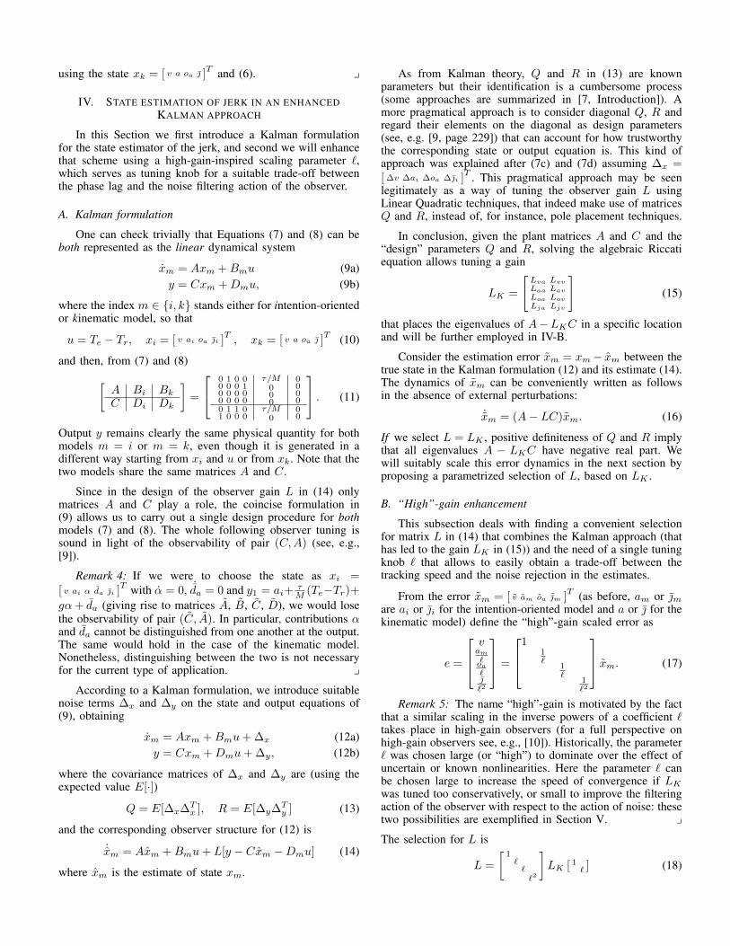
Mainly to illustrate the whole dataset, we depict in Figure 1the quantity oa

g180◦

π , i.e. the (normalized) estimated accelerom-eter offset converted in degrees. The light blue parts correspondto the time intervals when a gear change occurs: the darkerareas correspond to the times when the clutch is disengagedfrom the engine, the lighter areas correspond to re-engagement.The periodicity in the depicted signal is related to the two

0 50 100 150 200 250−8

−6

−4

−2

0

2

4

6

oa (

de

g)

t (s)

int, ell=2

int, ell=1.4

int, ell=0.8

Figure 1: (Normalized) estimated offset oa for the intention-oriented (int) model for different values of knob ` (ell).

track laps. The three different curves correspond to the threedifferent values of ` = 2, 1.4, 0.8.

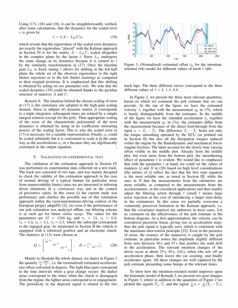
In Figure 2, we present the three most relevant quantities,based on which we comment the jerk estimate that we canprovide. At the top of the figure we have the estimatedvelocity v, together with the measurement y2 in (7f), whichis barely distinguishable from the estimates. In the middleof the figure we have the intended acceleration ai togetherwith the measurement y1 in (7e): the estimates differ fromthe measurement because of the direct feed-through from theinput u = Te − Tr. The difference Te − Tr bears not onlythe torque smoothing operated by the ECU (as pointed outin Section II) but also all the dissipation torques inducedwithin the engine by the fluidodynamic and mechanical forces(engine friction). The latter account for the slowly time varyingoffset visible in the middle plot. Already from the middleplot, but even more from the bottom plot, the smootheningeffect of parameter ` is evident. We would like to emphasizethat with the parameter ` at hand, we could set the values ofmatrices Q and R in (20) based on high level considerations(the entries of Q reflect the fact that the first state equationis the most reliable one, as noted in Section III, while theones in R that the measurements from the odometers aremore reliable, as compared to the measurements from theaccelerometers, in the considered application) and then readilyadjust the filtering action through ` (small ` means largenoise rejection at the cost of introducing a larger time-delayin the estimation). In this sense we partially overcome acommonly perceived limitation in the Kalman approach, i.e.that the covariance matrices are unknown in most cases. Letus comment on the effectiveness of the jerk estimate in thebottom diagram. As a first approximation, the velocity can beconsidered piecewise linear, giving rise to acceleration steps:thus the jerk signal is typically zero, which is consistent withthe minimum intervention principle [22]. Even in the presenceof noise, the essence of the maneuver is caught by the jerkestimate: in particular notice the amplitude slightly differentfrom zero between 80 s and 87 s that justifies the mild driftin the acceleration. The relevant intention changes of thedriver occur at about 78 s, 88 s, 102 s, when s/he sets off anacceleration phase, then leaves the car coasting, and finallyaccelerates again. All these changes are well captured by thejerk estimate presenting some bumps at the relevant times.

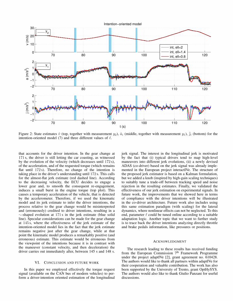
To show how the intention-oriented model improves uponthe kinematic model of Remark 3, we present two gear changesin Figure 3, where in addition to the quantities of Figure 2 weplotted the signals Te, Tr and the signal τ

M u = τM (Te − Tr),

70 80 90 100 110 1200

10

20

30Intention−oriented model

v (

m/s

)

y

2

70 80 90 100 110 120−2

−1

0

1

2

a (

m/s

2)

y

1

70 80 90 100 110 120−2

−1

0

1

2

t (s)

j (m

/s3)

int, ell=2

int, ell=1.4

int, ell=0.8

Figure 2: State estimates v (top, together with measurement y2), ai (middle, together with measurement y1), ˆi (bottom) for theintention-oriented model (7) and three different values of `.

that accounts for the driver intention. In the gear change at171 s, the driver is still letting the car coasting, as witnessedby the evolution of the velocity (which decreases until 172 s),of the acceleration, and of the requested torque (which remainsflat until 172 s). Therefore, no change of the intention istaking place in the driver’s understanding until 172 s. This callsfor the almost-flat jerk estimate (red dashed line). Accordingto the decreasing velocity, the ECU decides to engage alower gear and, to smooth the consequent re-engagement,induces a small burst in the engine torque (top plot). Thiscauses a temporary acceleration of the vehicle, that is detectedby the accelerometer. Therefore, if we used the kinematicmodel and its jerk estimate to infer the driver intentions, theprocess relative to the gear change would be misinterpretedand (erroneously) credited to driver intentions, resulting in a:-shaped evolution at 171 s in the jerk estimate (blue solidline). Specular considerations can be made for the gear changeat 145 s, where the effectiveness of the jerk estimate of theintention-oriented model lies in the fact that the jerk estimateremains negative just after the gear change, while at thatpoint the kinematic model produces a remarkably positive (anderroneous) estimate. This estimate would be erroneous fromthe viewpoint of the intentions because it is in contrast withthe maneuver (constant velocity, and then deceleration) thedriver carries out immediately after, between 145 s and 148 s.

VI. CONCLUSION AND FUTURE WORK

In this paper we employed effectively the torque requestsignal (available on the CAN bus of modern vehicles) to per-form a driver-intention oriented estimation of the longitudinal

jerk signal. The interest in the longitudinal jerk is motivatedby the fact that (i) typical drivers tend to map high-levelmaneuvers into different jerk evolutions, (ii) a newly devisedADAS (co-driver) based on the jerk signal was already imple-mented in the European project interactIVe. The structure ofthe proposed jerk estimator is based on a Kalman formulation,but we added a knob (inspired by high-gain scaling techniques)to suitably tune a trade-off between tracking speed and noiserejection in the resulting estimates. Finally, we validated theeffectiveness of our jerk estimation on experimental signals. Infuture work, the improvements that we showed here in termsof compliance with the driver intentions will be illustratedin the co-driver architecture. Future work also includes usingthis same estimation paradigm (with scaling) for the lateraldynamics, where nonlinear effects can not be neglected. To thisend, parameter ` could be tuned online according to a suitableadaptation logic. Another topic that we want to further studyis to trace back the driver intentions analyzing directly throttleand brake pedals information, like pressures or positions.

ACKNOWLEDGMENT

The research leading to these results has received fundingfrom the European Commission 7th Framework Programmeunder the project adaptIVe [2], grant agreement no. 610428.The authors would like to thank all partners within adaptIVe fortheir cooperation and valuable contribution. The work has alsobeen supported by the University of Trento, grant OptHySYS.The authors would also like to thank Giulio Panzani for usefuldiscussions.

135 140 145 150 155−100

0

100

200

Kinematic and intention model

T (

Nm

), (

Nm

/kg)

Te

Tr

100 τ/M u

135 140 145 150 15510

15

20

25

v (

m/s

)

y2

kin, ell=1.4

int, ell=1.4

135 140 145 150 155−2

0

2

a (

m/s

2)

y1

kin, ell=1.4

int, ell=1.4

135 140 145 150 155

−1

0

1

t (s)

j (m

/s3)

kin, ell=1.4

int, ell=1.4

166 168 170 172 174 176−50

0

50

100

150Kinematic and intention model

T (

Nm

), (

Nm

/kg

)

T

e

Tr

100 τ/M u

166 168 170 172 174 17615

20

25

v (

m/s

)

y

2

kin, ell=1.4

int, ell=1.4

166 168 170 172 174 176−1

0

1

a (

m/s

2)

y

1

kin, ell=1.4

int, ell=1.4

166 168 170 172 174 176−1

0

1

t (s)

j (m

/s3)

kin, ell=1.4

int, ell=1.4

Figure 3: Illustrative transitions corresponding to two gear changes for the intention-oriented model (7) and the kinematic one(8) with fixed ` = 1.4: torque signals Te, Tr, τ

M u (first from top), v and y2 (second), ai, a and y1 (third), ˆi and ˆ (fourth).

REFERENCES

[1] “interactIVe: accident avoidance by intervention for IntelligentVehicles,” Online resource, 2010-2013, available at http://www.interactive-ip.eu/ [Accessed April 26, 2015].

[2] “adaptIVe: Automated Driving Applications and Technologies for In-telligent Vehicles,” Online resource, 2014-, available at http://www.adaptive-ip.eu/ [Accessed April 26, 2015].

[3] R. Brooks, “A robust layered control system for a mobile robot,”Robotics and Automation, IEEE Journal of, vol. 2, no. 1, pp. 14–23,1986.

[4] Y. Chitour, “Time-varying high-gain observers for numerical differen-tiation,” Automatic Control, IEEE Transactions on, vol. 47, no. 9, pp.1565–1569, 2002.

[5] M. Da Lio, F. Biral, E. Bertolazzi, M. Galvani, P. Bosetti, D. Windridge,A. Saroldi, and F. Tango, “Artificial co-drivers as a universal enablingtechnology for future intelligent vehicles and transportation systems,”Intelligent Transportation Systems, IEEE Transactions on, vol. 16, no. 1,pp. 244–263, 2015.

[6] A. M. Dabroom and H. K. Khalil, “Discrete-time implementation ofhigh-gain observers for numerical differentiation,” International Journalof Control, vol. 72, no. 17, pp. 1523–1537, 1999.

[7] S. Formentin and S. Bittanti, “An insight into noise covariance es-timation for Kalman filter design,” in 19th World Congress of theInternational Federation of Automatic Control, vol. 19, no. 1, 2014,pp. 2358–2363.

[8] G. F. Fowler, R. E. Larson, and L. A. Wojcik, “Driver crash avoidancebehavior: Analysis of experimental data collected in NHTSA’s vehicleantilock brake system (ABS) research program,” SAE Technical Paper,Tech. Rep., 2005.

[9] J. P. Hespanha, Linear Systems Theory. Princeton, New Jersey:Princeton Press, 2009.

[10] H. K. Khalil and L. Praly, “High-gain observers in nonlinear feed-back control,” International Journal of Robust and Nonlinear Control,vol. 24, no. 6, pp. 993–1015, 2014.

[11] M. Klomp, Y. Gao, and F. Bruzelius, “Longitudinal velocity and roadslope estimation in hybrid electric vehicles employing early detectionof excessive wheel slip,” Vehicle System Dynamics, vol. 52, no. sup1,pp. 172–188, 2014.

[12] C. C. Macadam, “Understanding and modeling the human driver,”Vehicle System Dynamics, vol. 40, no. 1-3, pp. 101–134, 2003.

[13] J.-J. Martinez and C. Canudas-de Wit, “A safe longitudinal controlfor adaptive cruise control and stop-and-go scenarios,” Control SystemsTechnology, IEEE Transactions on, vol. 15, no. 2, pp. 246–258, 2007.

[14] L. Morales-Velazquez, R. de Jesus Romero-Troncoso, R. A. Osornio-Rios, and E. Cabal-Yepez, “Sensorless jerk monitoring using an adaptiveantisymmetric high-order FIR filter,” Mechanical Systems and SignalProcessing, vol. 23, no. 7, pp. 2383 – 2394, 2009.

[15] S.-i. Nakazawa, T. Ishihara, and H. Inooka, “Real-time algorithms forestimating jerk signals from noisy acceleration data,” InternationalJournal of Applied Electromagnetics and Mechanics, vol. 18, no. 1,pp. 149–163, 2003.

[16] M. Plochl and J. Edelmann, “Driver models in automobile dynamicsapplication,” Vehicle System Dynamics, vol. 45, no. 7-8, pp. 699–741,2007.

[17] J. J. Rangel-Magdaleno, R. J. Romero-Troncoso, R. A. Osornio-Rios,and E. Cabal-Yepez, “Novel oversampling technique for improvingsignal-to-quantization noise ratio on accelerometer-based smart jerksensors in CNC applications,” Sensors, vol. 9, no. 5, pp. 3767–3789,2009.

[18] Y. Sebsadji, S. Glaser, S. Mammar, and J. Dakhlallah, “Road slope andvehicle dynamics estimation,” in American Control Conference, 2008,2008, pp. 4603–4608.

[19] E. Todorov and M. I. Jordan, “A minimal intervention principle forcoordinated movement,” in Proc. Adv. Neural Inf. Process. Syst., vol. 15,2003, pp. 27–34.

[20] M. Yamakado and M. Abe, “An experimentally confirmed driverlongitudinal acceleration control model combined with vehicle lateralmotion,” Vehicle System Dynamics, vol. 46, no. sup1, pp. 129–149,2008.

[21] M. Yamakado and Y. Kadomukai, “A jerk sensor and its applicationto vehicle motion control systems,” in Proceedings of InternationalSymposium of Automotive Technology & Automation, vol. 27, 1994.

[22] M. Yamakado and M. Abe, “Examination of voluntary driving oper-ational timing by using information obtained with the developed jerksensor,” in FISITA 2006, 2006.

[23] M. Yamakado, J. Takahashi, S. Saito, A. Yokoyama, and M. Abe,“Improvement in vehicle agility and stability by G-Vectoring control,”Vehicle System Dynamics, vol. 48, no. sup1, pp. 231–254, 2010.