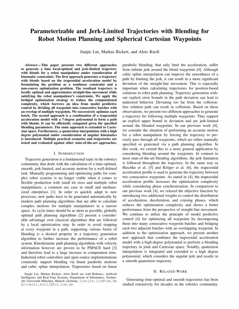
Parameterizable and Jerk-Limited Trajectories with Blending forRobot Motion Planning and Spherical Cartesian Waypoints

Jianjie Lin, Markus Rickert, and Alois Knoll

Abstract— This paper presents two different approachesto generate a time local-optimal and jerk-limited trajectorywith blends for a robot manipulator under consideration ofkinematic constraints. The first approach generates a trajectorywith blends based on the trapezoidal acceleration model byformulating the problem as a nonlinear constraint and anon-convex optimization problem. The resultant trajectory islocally optimal and approximates straight-line movement whilesatisfying the robot manipulator’s constraints. We apply thebridged optimization strategy to reduce the computationalcomplexity, which borrows an idea from model predictivecontrol by dividing all waypoints into consecutive batches withan overlap of multiple waypoints. We successively optimize eachbatch. The second approach is a combination of a trapezoidalacceleration model with a 7-degree polynomial to form a pathwith blends. It can be efficiently computed given the specifiedblending parameters. The same approach is extended to Carte-sian space. Furthermore, a quaternion interpolation with a highdegree polynomial under consideration of angular kinematicsis introduced. Multiple practical scenarios and trajectories aretested and evaluated against other state-of-the-art approaches.

I. INTRODUCTION

Trajectory generation is a fundamental topic in the roboticscommunity that deals with the calculation of a time-optimal,smooth, jerk-limited, and accurate motion for a well-definedtask. Manually programming and optimizing paths for com-plex robot systems is no longer viable when it comes toflexible production with small lot sizes and multiple robotmanipulators, a common use case in small and medium-sized enterprises [1]. In order to quickly adapt to newprocesses, new paths have to be generated automatically bymodern path planning algorithms that are able to calculatecomplex motions for multiple manipulators in a narrowspace. As cycle times should be as short as possible, globallyoptimal path planning algorithms [2] present a consider-able advantage over classical algorithms that are followedby a local optimization step. In order to avoid stoppingat every waypoint in a path, supporting various forms ofblending is a desired property in a trajectory generationalgorithm to further increase the performance of a robotsystem. Kinodynamic path planning algorithms with velocityinformation however are proven to be PSPACE hard [3]and therefore lead to a large increase in computation time.Industrial robot controllers and open-source implementationscommonly support blending via linear parabolic motionsand cubic spline interpolation. Trajectories based on linear

Jianjie Lin, Markus Rickert, Alois Knoll are with Robotics, ArtificialIntelligence and Real-Time Systems, Department of Informatics, Technis-che Universitat Munchen, Munich, Germany jianjie.lin@tum.de{rickert,knoll}@in.tum.de

parabolic blending, that only limit the acceleration, sufferfrom infinite jerk around the blend waypoints [4]. Althoughcubic spline interpolation can improve the smoothness of apath by limiting the jerk, it can result in a more significantdeviation of the straight-line movement. This is especiallyimportant when calculating trajectories for position-basedsolutions in robot path planning. Trajectory generation with-out explicit error bounds in the path deviation can lead toundesired behavior. Deviating too far from the collision-free solution path can result in collisions. Based on theseobservations, we present two different approaches to generatea trajectory for following multiple waypoints. They supportan explicit upper bound in deviation and are jerk-limitedaround the blended waypoints. In our previous work [4],we consider the situation of performing an accurate motionfor a robot manipulator by forcing the trajectory to pre-cisely pass through all waypoints, which are either manuallyspecified or generated via a path planning algorithm. Inthis work, we extend this to a more general application byconsidering blending around the waypoints. In contrast tomost state-of-the-art blending algorithms, the jerk limitationis followed throughout the trajectory. In the same way asHaschke et al. [5] and Kroger et al. [6], the trapezoidalacceleration profile is used to generate the trajectory betweentwo consecutive waypoints. As stated in [4], the trapezoidalacceleration profile increases the optimization complexitywhile considering phase synchronization. In comparison toour previous work [4], we relaxed the objective function byintroducing two additional weights to control the distributionof acceleration, deceleration, and cruising phases, whichreduces the optimization complexity and shows a betterperformance from the perspective of straight-line movement.We continue to utilize the principle of model predictivecontrol [4] for optimizing all waypoints by decomposingthem into many consecutive waypoint batches and bridgingeach two adjacent batches with an overlapping waypoint. Inaddition to the optimization approach, we present anothernew approach that combines the trapezoidal accelerationmodel with a high-degree polynomial to perform a blendingtrajectory in joint and Cartesian space. Notably, quaternioninterpolation is integrated and extended to a high degreepolynomial, which considers the angular jerk and results ina smooth quaternion trajectory.

II. RELATED WORK

Generating time-optimal and smooth trajectories has beenstudied extensively for decades in the robotics community.

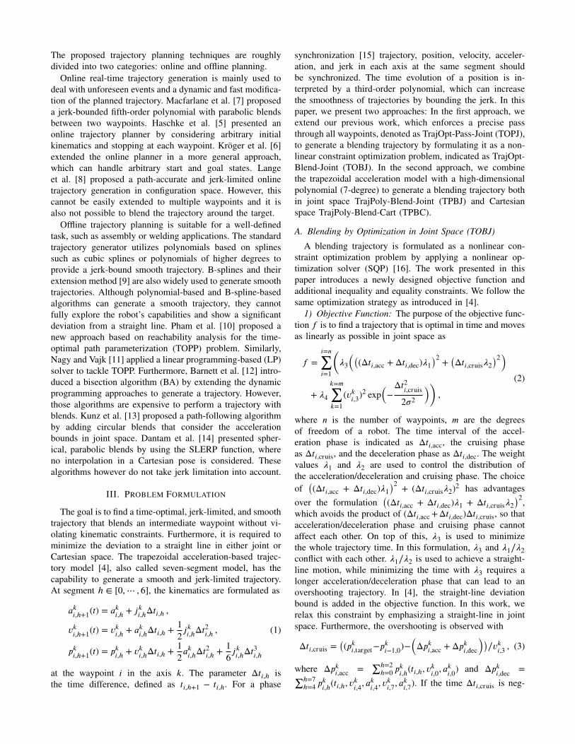
The proposed trajectory planning techniques are roughlydivided into two categories: online and offline planning.

Online real-time trajectory generation is mainly used todeal with unforeseen events and a dynamic and fast modifica-tion of the planned trajectory. Macfarlane et al. [7] proposeda jerk-bounded fifth-order polynomial with parabolic blendsbetween two waypoints. Haschke et al. [5] presented anonline trajectory planner by considering arbitrary initialkinematics and stopping at each waypoint. Kroger et al. [6]extended the online planner in a more general approach,which can handle arbitrary start and goal states. Langeet al. [8] proposed a path-accurate and jerk-limited onlinetrajectory generation in configuration space. However, thiscannot be easily extended to multiple waypoints and it isalso not possible to blend the trajectory around the target.

Offline trajectory planning is suitable for a well-definedtask, such as assembly or welding applications. The standardtrajectory generator utilizes polynomials based on splinessuch as cubic splines or polynomials of higher degrees toprovide a jerk-bound smooth trajectory. B-splines and theirextension method [9] are also widely used to generate smoothtrajectories. Although polynomial-based and B-spline-basedalgorithms can generate a smooth trajectory, they cannotfully explore the robot’s capabilities and show a significantdeviation from a straight line. Pham et al. [10] proposed anew approach based on reachability analysis for the time-optimal path parameterization (TOPP) problem. Similarly,Nagy and Vajk [11] applied a linear programming-based (LP)solver to tackle TOPP. Furthermore, Barnett et al. [12] intro-duced a bisection algorithm (BA) by extending the dynamicprogramming approaches to generate a trajectory. However,those algorithms are expensive to perform a trajectory withblends. Kunz et al. [13] proposed a path-following algorithmby adding circular blends that consider the accelerationbounds in joint space. Dantam et al. [14] presented spher-ical, parabolic blends by using the SLERP function, whereno interpolation in a Cartesian pose is considered. Thesealgorithms however do not take jerk limitation into account.

III. PROBLEM FORMULATION

The goal is to find a time-optimal, jerk-limited, and smoothtrajectory that blends an intermediate waypoint without vi-olating kinematic constraints. Furthermore, it is required tominimize the deviation to a straight line in either joint orCartesian space. The trapezoidal acceleration-based trajec-tory model [4], also called seven-segment model, has thecapability to generate a smooth and jerk-limited trajectory.At segment ℎ ∈ [0,⋯ , 6], the kinematics are formulated as

aki,ℎ+1(t) = aki,ℎ + j

ki,ℎΔti,ℎ ,

vki,ℎ+1(t) = vki,ℎ + a

ki,ℎΔti,ℎ +

12jki,ℎΔt

2i,ℎ , (1)

pki,ℎ+1(t) = pki,ℎ + v

ki,ℎΔti,ℎ +

12aki,ℎΔt

2i,ℎ +

16jki,ℎΔt

3i,ℎ

at the waypoint i in the axis k. The parameter Δti,ℎ isthe time difference, defined as ti,ℎ+1 − ti,ℎ. For a phase

synchronization [15] trajectory, position, velocity, acceler-ation, and jerk in each axis at the same segment shouldbe synchronized. The time evolution of a position is in-terpreted by a third-order polynomial, which can increasethe smoothness of trajectories by bounding the jerk. In thispaper, we present two approaches: In the first approach, weextend our previous work, which enforces a precise passthrough all waypoints, denoted as TrajOpt-Pass-Joint (TOPJ),to generate a blending trajectory by formulating it as a non-linear constraint optimization problem, indicated as TrajOpt-Blend-Joint (TOBJ). In the second approach, we combinethe trapezoidal acceleration model with a high-dimensionalpolynomial (7-degree) to generate a blending trajectory bothin joint space TrajPoly-Blend-Joint (TPBJ) and Cartesianspace TrajPoly-Blend-Cart (TPBC).

A. Blending by Optimization in Joint Space (TOBJ)

A blending trajectory is formulated as a nonlinear con-straint optimization problem by applying a nonlinear op-timization solver (SQP) [16]. The work presented in thispaper introduces a newly designed objective function andadditional inequality and equality constraints. We follow thesame optimization strategy as introduced in [4].

1) Objective Function: The purpose of the objective func-tion f is to find a trajectory that is optimal in time and movesas linearly as possible in joint space as

f =i=n∑

i=1

(

�3(

(

(Δti,acc + Δti,dec)�1)2 +

(

Δti,cruis�2)2)

+ �4k=m∑

k=1(vki,3)

2 exp(

−Δt2i,cruis2�2

)

)

,

(2)

where n is the number of waypoints, m are the degreesof freedom of a robot. The time interval of the accel-eration phase is indicated as Δti,acc, the cruising phaseas Δti,cruis, and the deceleration phase as Δti,dec. The weightvalues �1 and �2 are used to control the distribution ofthe acceleration/deceleration and cruising phase. The choiceof

(

(Δti,acc + Δti,dec)�1)2 + (Δti,cruis�2)2 has advantages

over the formulation(

(Δti,acc + Δti,dec)�1 + Δti,cruis�2)2,

which avoids the product of (Δti,acc+Δti,dec)Δti,cruis, so thatacceleration/deceleration phase and cruising phase cannotaffect each other. On top of this, �3 is used to minimizethe whole trajectory time. In this formulation, �3 and �1∕�2conflict with each other. �1∕�2 is used to achieve a straight-line motion, while minimizing the time with �3 requires alonger acceleration/deceleration phase that can lead to anovershooting trajectory. In [4], the straight-line deviationbound is added in the objective function. In this work, werelax this constraint by emphasizing a straight-line in jointspace. Furthermore, the overshooting is observed with

Δti,cruis =(

(pki,target−pki−1,0)−

(

Δpki,acc + Δpki,dec

)

)

∕vki,3 , (3)

where Δpki,acc =∑ℎ=2ℎ=0 p

ki,ℎ(ti,ℎ, v

ki,0, a

ki,0) and Δpki,dec =

∑ℎ=7ℎ=4 p

ki,ℎ(ti,ℎ, v

ki,4, a

ki,4, v

ki,7, a

ki,7). If the time Δti,cruis is neg-

ative, the reached position overshoots the target. To elim-inate this undesired behavior, the cruising phase shouldbe omitted. Since Δpki,acc + Δp

ki,dec has a longer distance

than pki,target − pki−1,0, we can reduce the cruising veloc-ity vki,3 to shorten Δpki,acc. Besides, the trapezoidal endvelocity vi,7 influences the position Δpki,dec, which can beautomatically tuned by the optimization solver. We add a

regular term (vki,3)2 exp(−

Δt2i,cruis2�2 ) in the objective function

with �, which controls the decay rate. It can be shown

that at Δti,cruis ≈ 0, the regular term (vki,3)2 exp(−

Δt2i,cruis2�2 )

is approximated as (vki,3)2, and the velocity is reduced by

minimizing the objective function. In the case of Δti,cruis > 0,

the Gaussian value exp(−Δt2i,cruis2�2 ) is exponentially decayed to

zero, which has no effect on the cruising phase.2) Kinematic Constraints: Instead of passing through

the waypoints, we define a blending bound between twoconsecutive line segments. Furthermore, we set a non-zerovelocity and acceleration for each waypoint, except for thefirst and last waypoint. The constraints are described as

pk(ti,ℎ1 ) = pki+1,bl,start , ℎ1 ∈ [4,… , 6] ,

pk(ti+1,ℎ2 ) = pki+1,bl,end , ℎ2 ∈ [0,… , 3] ,

vk(t0,0) = vk(tn,0) = 0, Δti,ℎ ≥ 0 ,ak(t0,0) = ak(tn,0) = ak(ti,3) = 0 ,|jk(ti,ℎ)| ≤ jkmax , |a

k(ti,ℎ)| ≤ akmax ,∀ℎ ∈ [0,… , 6]|vk(ti,ℎ)| ≤ vkmax , |p

k(ti,ℎ)| ≤ pkmax ,∀ℎ ∈ [0,… , 6]pki,bl,lower ≤ pki+1,bl ≤ pki+1,bl,upper ,

(4)

where pki+1,bl,start is the start blending segment position atwaypoint i + 1 in axis k and pki+1,bl,end is the end blendingsegment position at waypoint i + 1 in axis k. The vari-able pki,bl,lower , p

ki,bl,upper is a lower and upper blending bound,

respectively. The corresponding optimized blending way-point at i + 1 in axis k is indicated as pki+1,bl. The variable ℎ1and ℎ2 are predefined values that depend on the blendingpercentage. One relaxation of the jerk j constraint [5] ismade by allowing double acceleration or deceleration phases:sign(j) is no longer strictly defined as [±, 0,∓, 0,∓, 0,±]but changed to sign(j) = [±, 0,±, 0,±, 0,±]. This relaxationallows reaching the next waypoint without slowing down.

3) Blending Bound Constraints: The blending con-straint pi,bl,con is computed as pi+1+ yr�, where y is definedas y2−y1

‖y2−y1‖with y1 = pi+1−pi

‖pi+1−pi‖and y2 = pi+2−pi+1

‖pi+2−pi+1‖.

Additionally, r = li∕(tan �i+1∕2) with �i+1 = arccos(yT1 y2)and li = min

{

‖pi+1−pi‖2 , ‖pi+2−pi+1‖2 , � sin(�i+1∕2)

(1−cos(�i+1∕2))

}

, where �is the predefined blending distance from qi+1. � is the per-centage value for controlling the blending bound. The devi-ation �bl = ‖

‖

pi,bl,con − p(ti,7)‖‖ is bound. Utilizing the blend-ing constraints, we have pki,bl,lower = min{pki,bl,con, p

k(ti,7)}and pki,bl,upper = max{p

ki,bl,con, p

k(ti,7)}.

B. Blending with Polynomial in Joint Space (TPBJ)

The second approach combines the trapezoidal with ahigh-dimensional polynomial to form a blending path. Theblending segment is described as a high-degree polynomialunder consideration of initial f0 = (p0, v0, a0, j0) andfinal f1 = (p1, v1, a1, j1) kinematic constraints. Theserequire a total of eight coefficients, therefore we utilizea 7-degree polynomial function in one dimension: f (t) =b7t7 + b6t6 +⋯ + b2t2 + b1t + b0. The coefficients b0 - b3can be computed using f0 with b0 = p0, b1 = v0, b2 =

a02

and b3 =j06 . The coefficients b4 to b7 depending on f1 and

polynomial time t can be described as

⎡

⎢

⎢

⎢

⎣

t71 t61 t51 t417t61 6t51 5t41 4t3142t51 30t41 20t31 12t

21

210t41 120t31 60t

21 24t1

⎤

⎥

⎥

⎥

⎦

⏟⏞⏞⏞⏞⏞⏞⏞⏞⏞⏞⏞⏟⏞⏞⏞⏞⏞⏞⏞⏞⏞⏞⏞⏟A1

[ b7b6b5b4

]

⏟⏟⏟x1

=[ p1v1a1j1

]

⏟⏟⏟y1

−⎡

⎢

⎢

⎣

1 t11 t21 t310 1 2t1 3t210 0 2 6t10 0 0 6

⎤

⎥

⎥

⎦

⏟⏞⏞⏞⏞⏟⏞⏞⏞⏞⏟A2

[ b0b1b2b3

]

⏟⏟⏟y2

.

Due to this, x1(t1, f0, f1) = A−11 (y1 − A2y2) with timematrices A1, A2. The polynomial is simplified as

f (t, f0, f1) = [t7, t6, t5, t4]x1(t1, f0, f1) + ℎ2(t, f0) , (5)

where ℎ2(t, f0) is described as 16 j0t

3 + 12a0t

2 + v0t + p0.Firstly, we assume that the initial f0 and final f1 kinematicconstraints are available. Therefore, f (t) depends only on thetime t. To find a polynomial blending trajectory that satisfiesall kinematic constraints, we need to verify the extreme pointof the polynomial by computing the root of its derivative.For example, the extreme point of jerk can be found at theposition where the first derivative of the jerk (snap) is equalto zero. In addition, a n-degree polynomial has at most n realroots. The constraints can be mathematically formulated as

|f (n−1)(�(f (n)))��(�(f (n)))| ≤ kmax , (6)

where f (n) is n-th derivative of f with n ∈ [1, 4] and thecorresponding constraints kmax ∈ [pmax, vmax, amax, jmax].The root-finding function �(f (n)) for a given polynomial isused to find the extreme value position for f (n−1). �A(x) isthe indicator function of A and will be set to one if x ∈[0, t], otherwise to zero. Note that if the �A(x) functionis not derivable, the gradient-based optimization solver willdiverge. To find a time-optimal polynomial trajectory thatsatisfies initial/final conditions and lies within the kinematicconstraints, we iteratively check the constraints (6) by addinga small delta to t = t + Δt, where in our case Δt is setto 0.001. Furthermore, to obtain the initial f0 and final f1kinematics, we compute a Point to Point (P2P) trapezoidalacceleration profile movement between each two waypoints,which can be in joint space or Cartesian space, with zeroinitial and end conditions, and the computed traveling timeis indicated as ti−>i+1. After that, we predefine a blendingpercentage � to set a start blending time tbstart = (1−�)ti−>i+1and end blending time tbend = �ti+1−>i+2 for each twoconsecutive trajectories. By querying the trapezoidal modelat tbstart and tbend , we obtain the kinematics f0 and f1.

C. Blending with Polynomial in Cartesian Space (TPBC)

Utilizing the same principle, we extend the algorithm tothe Cartesian space, which is widely used in industrial appli-cations. The blending trajectory in Cartesian space requiresseparate blending for position and orientation. Interpolationof the Cartesian space is executed in the same way as de-scribed in Section III-B. For the orientation part, which has toconsider a spherical interpolation, we apply the formulation:

h(t) = hiΔh(t) = hi(

u(t) sin(�(t)∕2)cos(�(t)∕2) ,

)

(7)

where hi is the initial quaternion, and Δh(t) transforms thequaternion from hi to h(t). The Eigen axis between twoquaternions is defined as u(t) = �(t)∕ ‖�(t)‖ ∈ 3 with arotation angle �(t) = ‖�(t)‖. Therefore, the quaternion inter-polation depends only on �(t) ∈ 3. To consider the angularvelocity !, angular acceleration !, and angular jerk ! atthe start and end state for the quaternion blending, the timeevolution function �(t) is described as: �(t) = a1(x − 1)7 +a2x(x−1)6+⋯+a8x7 with x = t

tf−t0∈ [0, 1]. Its roots and

its derivative are computed at point x = 0 and x = 1. Basedon h = 1

2h!, we can derive the relationship between ! ∈ 3

and � ∈ 3 as ! = u� + sin(�)w × u − (1 − cos(�))w,where w = (u×�)

� ∈ 3 and � = uT � is a scalar value. Wefurther simplify ! with the skew-symmetric matrix (⋅)× as! = (uuT − sin(�)

� u×u× − (1−cos(�))� u×)� = A!,1�. In the same

way, we can compute the angular acceleration ! and jerk !.We combine Cartesian position and quaternion interpolationto form a trajectory with blends.

IV. EXPERIMENTAL EVALUATION

We compare the performance of the presented approachesin this paper with the work by Kunz et al. [13] (TO-BAV),Pham et al. [10] (TOPP-RA) and our previous work [4].The work in [13] generates a trajectory with a designed cir-cular blend under consideration of velocity and accelerationbounds and the work [10] used the reachability-analysis (RA)to solve the time optimal path parameterization (TOPP)problem. Our previous work [4] generates a trajectory byforcing a precise pass through all desired waypoints withoutstopping. For the evaluation of the motion planning scene,the collision-free paths in the examples are computed usingthe Robotics Library [17], which is also used for kinematiccalculations and simulation. In the evaluation, we set theweights in [4] and TOBJ as �1 = 1.2, �2 = 1, �3 = 5000,and �4 = 10. All evaluations were performed on a laptopwith a 2.6GHz Intel Core i7-6700HQ and 16GB of RAM.

A. Evaluation of Deviation from Straight-Line in Joint Space

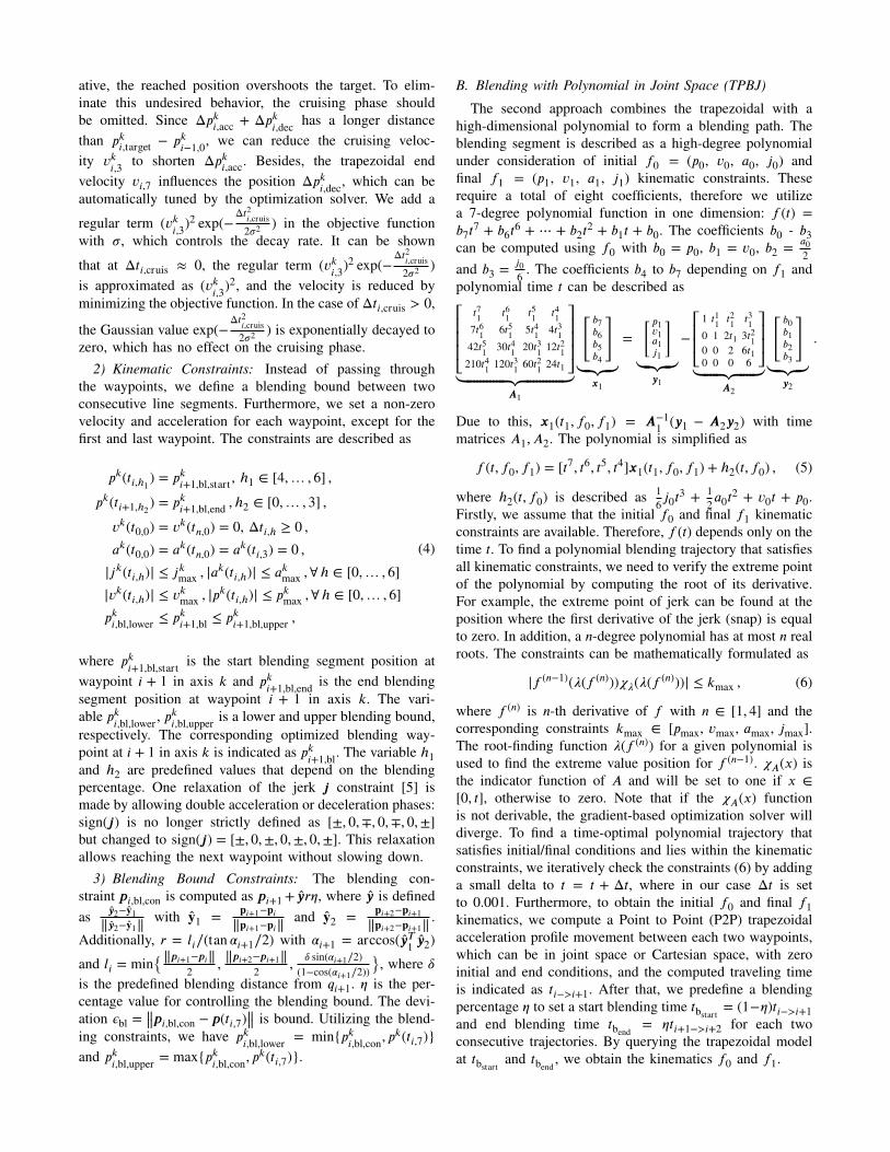
For the first evaluation, we consider a subset of the well-known ISO 9283 [18] cube industrial benchmark as shown inFig. 1. Here, the robot’s end effector has to follow a numberof waypoints that are part of a two-dimensional rectangleinside a three-dimensional cube while applying blending.The corresponding results are shown in Fig. 1. The previouswork TOPJ [4] in Fig. 1a completed the ISO cube task

within 6.26 s by passing through all waypoints and the gener-ated trajectory has to deviate from the straight-line movementto avoid stopping at each waypoint. For improving the qualityof the trajectory, TOBJ presented in this work extends theTOPJ by blending around the target position, which resultsin a better straight-line movement and completed the ISOcube task with a shorter time of 6.1 s due to a shortenedpath length. The polynomial based algorithm (TPBJ) canfurther reduce the completion time to 5.94 s by setting abigger blending circle radius.

B. Comparison between TO-BAV, TOPP-RA and TPBJ

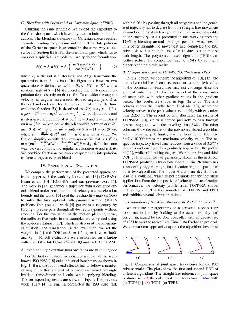
In this section, we compare the algorithm of [10], [13] andour polynomial-based one, as using an extreme jerk valuein the optimization-based one may not converge since thegradient value in jerk direction is not at the same orderof magnitude with other gradient values in the gradientvector. The results are shown in Figs. 2a to 2o. The firstcolumn shows the results from TO-BAV [13], where thevelocity arrives at the peak value very quickly with executiontime 2.2577 s. The second column illustrates the results ofTOPP-RA [10], which is forced precisely to pass throughdesired waypoints with the traveling time 2.88 s. The othercolumns show the results of the polynomial-based algorithmwith increasing jerk limits, starting from 5, to 100, andfinally 10 000 times the maximum velocity value. The re-spective trajectory travel time reduces from a value of 3.577 sto 2.28 s and our algorithm gradually approaches the profileof [13], while still limiting the jerk. We plot the first and thirdDOF path without loss of generality, shown in the first row.TOPP-RA produces a trajectory shown in Fig. 2b which hasa noticeably bigger straight-line deviation in joint space thanother two algorithms. The bigger straight-line deviation canlead to a collision, which is not desirable for the industrialapplication. From the perspective of velocity and accelerationperformance, the velocity profile from TOPP-RA shownin Figs. 2g and 2l is less smooth than TO-BAV and TPBJand exhibits several vibration points.

C. Evaluation of the Algorithm in a Real Robot Workcell

We evaluate our algorithms on a Universal Robots UR5robot manipulator by looking at the actual velocity andcurrent measured by the UR5 controller with an update rateof 125Hz over the native Real-Time Data Exchange protocol.We compare our approaches against the algorithm developed

(a) (b) (c)

Fig. 1: Comparison of joint space trajectories for the ISOcube scenario. The plots show the first and second DOF ofdifferent algorithms. The straight line reference in joint spaceis shown in red, the calculated joint trajectory in blue with(a) TOPJ [4], (b) TOBJ, (c) TPBJ.

(a) Pos. (TO-BAV) (b) Pos. (TOPP-RA) (c) Pos. (TPBJ) (d) Pos. (TPBJ) (e) Pos. (TPBJ)

0 s 2.257 s−2.6 rad∕s

2.2 rad∕s

(f) Vel. (TO-BAV)

0 s 2.887 s−2.7 rad∕s

2.2 rad∕s

(g) Vel. (TOPP-RA)

0 s 3.578 s

−1.31 rad∕s

1.13 rad∕s

(h) Vel. (TPBJ)

0 s 2.328 s−2.52 rad∕s

2.19 rad∕s

(i) Vel. (TPBJ)

0 s 2.28 s−2.25 rad∕s

1.94 rad∕s

(j) Vel. (TPBJ)

0 s 2.257 s−6.3 rad∕s2

6.3 rad∕s2

(k) Acc. (TO-BAV)

0 s 2.887 s−6.3 rad∕s2

6.3 rad∕s2

(l) Acc. (TOPP-RA)

0 s 3.578 s

−3.3 rad∕s24.17 rad∕s2

(m) Acc. (TPBJ)

0 s 2.328 s−6.9 rad∕s2

6.31 rad∕s2

(n) Acc. (TPBJ)

0 s 2.28 s−6.27 rad∕s2

6.32 rad∕s2

(o) Acc. (TPBJ)

Fig. 2: Comparison of results from TO-BAV [13], TOPP-RA [10] and TPBJ with increasing jerk constraints. (a)–(e) show theplot of first and third DOF with generated trajectory (blue) and target straight-line path (red). (f)–(j) is the velocity profile. (k)–(o) is the acceleration profile. In our approach, TPBJ gradually increases jerk constraints from jmax = {5, 100, 10000}vmax.

(a) TO-BAV (b) TOPJ (c) TOBJ (d) TPBJ (e) TPBC

0 s 3.30 s−1.8 rad∕s

1.6 rad∕s

(f) TO-BAV

0 s 3.83 s

−1.4 rad∕s

1.1 rad∕s

(g) TOPJ

0 s 3.80 s

−1.1 rad∕s

1.0 rad∕s

(h) TOBJ

0 s 3.56 s

−1.3 rad∕s

1.2 rad∕s

(i) TPBJ

0 s 4.36 s

−1.2 rad∕s

0.9 rad∕s

(j) TPBC

0 s 3.30 s−4 rad∕s

0 rad∕s

4 rad∕s ⋅10−2

(k) TO-BAV

0 s 3.83 s

−2 rad∕s0 rad∕s2 rad∕s

⋅10−2

(l) TOPJ

0 s 3.80 s

−2.1 rad∕s0 rad∕s

2.1 rad∕s⋅10−2

(m) TOBJ

0 s 3.56 s

−2.5 rad∕s0 rad∕s

2.5 rad∕s⋅10−2

(n) TPBJ

0 s 4.36 s

−2 rad∕s0 rad∕s2 rad∕s

⋅10−2

(o) TPBC

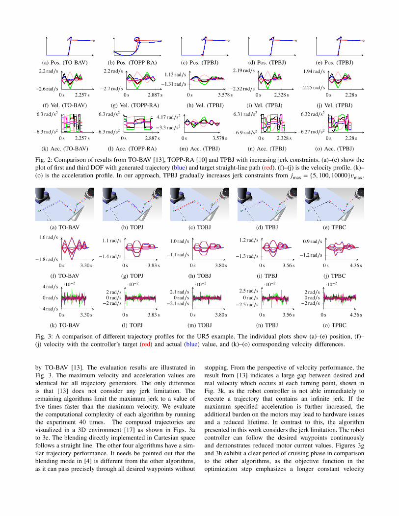
Fig. 3: A comparison of different trajectory profiles for the UR5 example. The individual plots show (a)–(e) position, (f)–(j) velocity with the controller’s target (red) and actual (blue) value, and (k)–(o) corresponding velocity differences.

by TO-BAV [13]. The evaluation results are illustrated inFig. 3. The maximum velocity and acceleration values areidentical for all trajectory generators. The only differenceis that [13] does not consider any jerk limitation. Theremaining algorithms limit the maximum jerk to a value offive times faster than the maximum velocity. We evaluatethe computational complexity of each algorithm by runningthe experiment 40 times. The computed trajectories arevisualized in a 3D environment [17] as shown in Figs. 3ato 3e. The blending directly implemented in Cartesian spacefollows a straight line. The other four algorithms have a sim-ilar trajectory performance. It needs be pointed out that theblending mode in [4] is different from the other algorithms,as it can pass precisely through all desired waypoints without

stopping. From the perspective of velocity performance, theresult from [13] indicates a large gap between desired andreal velocity which occurs at each turning point, shown inFig. 3k, as the robot controller is not able immediately toexecute a trajectory that contains an infinite jerk. If themaximum specified acceleration is further increased, theadditional burden on the motors may lead to hardware issuesand a reduced lifetime. In contrast to this, the algorithmpresented in this work considers the jerk limitation. The robotcontroller can follow the desired waypoints continuouslyand demonstrates reduced motor current values. Figures 3gand 3h exhibit a clear period of cruising phase in comparisonto the other algorithms, as the objective function in theoptimization step emphasizes a longer constant velocity

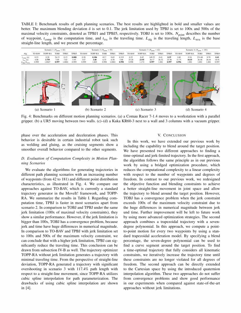
TABLE I: Benchmark results of path planning scenarios. The best results are highlighted in bold and smaller values arebetter. The maximum blending deviation � is set to 0.1. The jerk limitation used by TPBJ is set to 100x and 500x of themaximal velocity constraints, denoted as TPBJ1 and TPBJ5, respectively. TOBJ is set to 100x. Npoint describes the numberof waypoint, tcomp is the computation time, and ttra is the traveling time. Lalg is the traveling length, Lstra is the basestraight-line length, and we present the percentage.

Scenario 1 (Npoint = 42) Scenario 2 (Npoint = 55) Scenario 3 (Npoint = 42) Scenario 4 (Npoint = 181)

Alg. TO-BAV TOPP-RA TOBJ TPBJ1 TPBJ5 TO-BAV TOPP-RA TOBJ TPBJ1 TPBJ5 TO-BAV TOPP-RA TOBJ TPBJ1 TPBJ5 TO-BAV TOPP-RA TOBJ TPBJ1 TPBJ5

tcomp [s] 0.23 0.28 54.15 0.15 0.088 0.28 0.186 65.7 0.65 0.319 0.32 0.45 149.52 0.41 0.25 1.68 0.54 231.68 0.70 0.41ttra [s] 4.08 3.759 7.09 7.02 5.95 3.67 3.40 6.35 6.58 5.88 25.20 23.95 26.17 26.32 25.48 11.75 10.55 26.48 26.44 18.91

Lalg∕Lstra 0.999 1.0027 0.997 1.0001 0.999 0.999 1.003 0.998 1.0001 0.998 0.998 1.174 0.997 1.001 0.997 0.996 1.001 1.001 1.001 0.997

(a) Scenario 1 (b) Scenario 2 (c) Scenario 3 (d) Scenario 4

Fig. 4: Benchmarks on different motion planning scenarios. (a) a Comau Racer 7-1.4 moves to a workstation with a parallelgripper. (b) a UR5 moving between two walls. (c)–(d) a Kuka KR60-3 next to a wall and 3 columns with a vacuum gripper.

phase over the acceleration and deceleration phases. Thisbehavior is desirable in certain industrial robot task suchas welding and gluing, as the cruising segments show asmoother overall behavior compared to the other segments.

D. Evaluation of Computation Complexity in Motion Plan-ning Scenarios

We evaluate the algorithms for generating trajectories indifferent path planning scenarios with an increasing numberof waypoints (from 42 to 181) and different point distributioncharacteristics, as illustrated in Fig. 4. We compare ourapproaches against TO-BAV, which is currently a standardtrajectory generator in the MoveIt! framework, and TOPP-RA. We summarize the results in Table I. Regarding com-putation time, TPBJ is faster in most scenarios apart fromscenario 2. In comparison to TOBJ and TPBJ under the samejerk limitation (100x of maximal velocity constraints), theyshow a similar performance. However, if the jerk limitation isbigger than 100x, TOBJ has a convergence problem, becausejerk and time have huge differences in numerical magnitude.In comparison to TO-BAV and TPBJ with jerk limitation setto 100x and 500x of the maximum velocity constraint, wecan conclude that with a higher jerk limitation, TPBJ can sig-nificantly reduce the traveling time. This conclusion can bedrawn from subsection IV-B as well. The trajectory optimizerTOPP-RA without jerk limitation generates a trajectory withminimal traveling time. From the perspective of straight-linedeviation, TOPP-RA generated a trajectory with significantovershooting in scenario 3 with 117.4% path length withrespect to a straight-line movement, since TOPP-RA utilizescubic spline interpolation for path parameterization. Thedrawbacks of using cubic spline interpolation are shownin [4].

V. CONCLUSION

In this work, we have extended our previous work byincluding the capability to blend around the target position.We have presented two different approaches to finding atime-optimal and jerk-limited trajectory. In the first approach,the algorithm follows the same principle as in our previouswork by using a bridged optimization procedure, whichreduces the computational complexity to a linear complexitywith respect to the number of waypoints and degrees offreedom. In contrast to our previous work, we redesignedthe objective function and blending constraints to achievea better straight-line movement in joint space and allowthe trajectory to blend around the target position. However,TOBJ has a convergence problem when the jerk constraintexceeds 100x of the maximum velocity constraint due tothe huge differences in numerical magnitude between jerkund time. Further improvement will be left to future workby using more advanced optimization strategies. The secondapproach combines a trapezoidal trajectory with a seven-degree polynomial. In this approach, we compute a point-to-point motion for every two waypoints by using a stan-dard trapezoidal acceleration model. By specifying a blendpercentage, the seven-degree polynomial can be used tofind a curve segment around the target position. To finda time-optimal trajectory that fully considers all kinematicconstraints, we iteratively increase the trajectory time untilthese constraints are no longer violated for all degrees offreedom. The second approach can be directly extendedto the Cartesian space by using the introduced quaternioninterpolation algorithm. These two approaches do not sufferfrom convergence problems and show good performancein our experiments when compared against state-of-the-artapproaches without jerk limitations.

REFERENCES

[1] A. Perzylo, M. Rickert, B. Kahl, N. Somani, C. Lehmann, A. Kuss,S. Profanter, A. B. Beck, M. Haage, M. R. Hansen, M. T. Nibe, M. A.Roa, O. Sornmo, S. G. Robertz, U. Thomas, G. Veiga, E. A. Topp,I. Kesslar, and M. Danzer, “SMErobotics: Smart robots for flexiblemanufacturing,” IEEE Robotics and Automation Magazine, vol. 26,no. 1, pp. 78–90, Mar. 2019.

[2] E. F. Sertac Karaman, “Sampling-based algorithms for optimal motionplanning,” The International Journal of Robotics Research, vol. 30,no. 7, pp. 846–894, June 2011.

[3] B. Donald, P. Xavier, J. Canny, and J. Reif, “Kinodynamic motionplanning,” Journal of the ACM, vol. 40, no. 5, pp. 1048–1066, Nov.1993.

[4] J. Lin, N. Somani, B. Hu, M. Rickert, and A. Knoll, “An efficient andtime-optimal trajectory generation approach for waypoints under kine-matic constraints and error bounds,” in Proceedings of the IEEE/RSJInternational Conference on Intelligent Robots and Systems, Madrid,Spain, Oct. 2018, pp. 5869–5876.

[5] R. Haschke, E. Weitnauer, and H. Ritter, “On-line planning of time-optimal, jerk-limited trajectories,” in Proceedings of the IEEE/RSJInternational Conference on Intelligent Robots and Systems, Nice,France, Sept. 2008, pp. 3248–3253.

[6] T. Kroger and F. M. Wahl, “Online trajectory generation: Basicconcepts for instantaneous reactions to unforeseen events,” IEEETransactions on Robotics, vol. 26, no. 1, pp. 94–111, Feb. 2009.

[7] S. Macfarlane and E. A. Croft, “Jerk-bounded manipulator trajectoryplanning: Design for real-time applications,” IEEE Transactions onRobotics and Automation, vol. 19, no. 1, pp. 42–52, Feb. 2003.

[8] F. Lange and A. Albu-Schaffer, “Path-accurate online trajectory gen-eration for jerk-limited industrial robots,” IEEE Robotics and Automa-tion Letters, vol. 1, no. 1, pp. 82–89, Jan. 2016.

[9] R. Saravanan, S. Ramabalan, and C. Balamurugan, “Evolutionary op-timal trajectory planning for industrial robot with payload constraints,”The International Journal of Advanced Manufacturing Technology,vol. 38, pp. 1213–1226, Sept. 2008.

[10] H. Pham and Q.-C. Pham, “A new approach to time-optimal pathparameterization based on reachability analysis,” IEEE Transactionson Robotics, vol. 34, no. 3, pp. 645–659, June 2018.

[11] A. Nagy and I. Vajk, “Sequential time-optimal path-tracking algorithmfor robots,” IEEE Transactions on Robotics, vol. 35, no. 5, Oct. 2019.

[12] E. Barnett and C. Gosselin, “A bisection algorithm for time-optimaltrajectory planning along fully specified paths,” IEEE Transactions onRobotics, vol. 37, no. 1, pp. 1–15, Feb. 2021.

[13] T. Kunz and M. Stilman, “Time-optimal trajectory generation for pathfollowing with bounded acceleration and velocity,” Proceedings ofRobotics: Science and Systems, July 2012.

[14] N. Dantam and M. Stilman, “Spherical parabolic blends for robotworkspace trajectories,” in Proceedings of the IEEE/RSJ InternationalConference on Intelligent Robots and Systems, Chicago, IL, USA,Sept. 2014, pp. 3624–3629.

[15] T. Kroger, “Opening the door to new sensor-based robot applications—the Reflexxes motion libraries,” in Proceedings of the IEEE Interna-tional Conference on Robotics and Automation, Shanghai, China, May2011.

[16] J. Nocedal and S. Wright, Numerical optimization. Springer Science& Business Media, 2006.

[17] M. Rickert and A. Gaschler, “Robotics Library: An object-orientedapproach to robot applications,” in Proceedings of the IEEE/RSJ Int.Conf. on Intelligent Robots and Systems, Vancouver, BC, Canada, Sept.2017, pp. 733–740.

[18] “Manipulating industrial robots, Performance criteria and related testmethods,” ISO, International Standard 9283, Apr. 1998.