Transformation from 3D modelling to building information modelling
CITS3003 Graphics & Animation
Lecture: 3D Modelling
E. Angel and D. Shreiner: Interactive Computer Graphics 6E © Addison-Wesley 2012
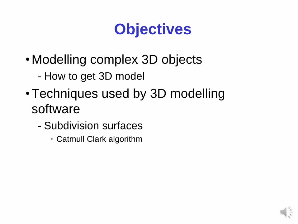
Objectives
•Modelling complex 3D objects
- How to get 3D model
•Techniques used by 3D modelling
software
- Subdivision surfaces• Catmull Clark algorithm
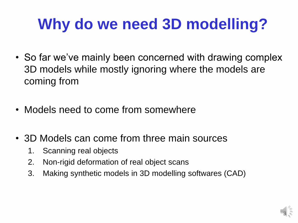
Why do we need 3D modelling?
• So far we’ve mainly been concerned with drawing complex
3D models while mostly ignoring where the models are
coming from
• Models need to come from somewhere
• 3D Models can come from three main sources
1. Scanning real objects
2. Non-rigid deformation of real object scans
3. Making synthetic models in 3D modelling softwares (CAD)
3
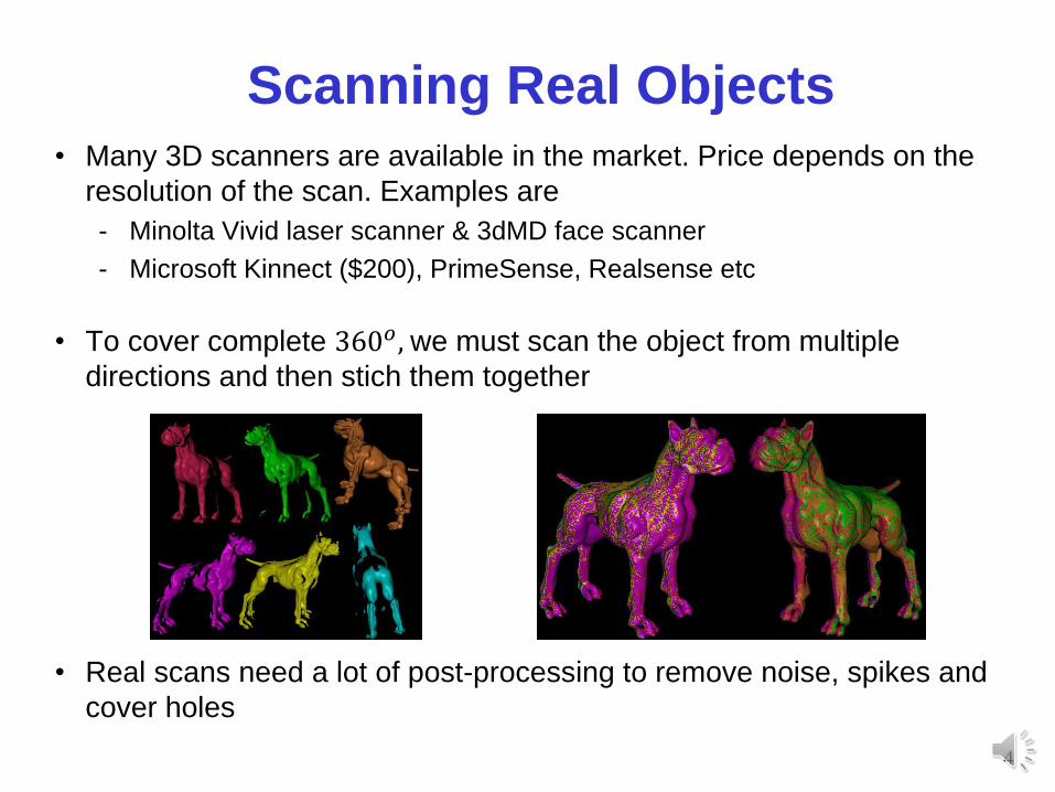
Scanning Real Objects• Many 3D scanners are available in the market. Price depends on the
resolution of the scan. Examples are
- Minolta Vivid laser scanner & 3dMD face scanner
- Microsoft Kinnect ($200), PrimeSense, Realsense etc
• To cover complete 360𝑜, we must scan the object from multiple
directions and then stich them together
• Real scans need a lot of post-processing to remove noise, spikes and
cover holes
4
Non-Rigid Deformation of Models
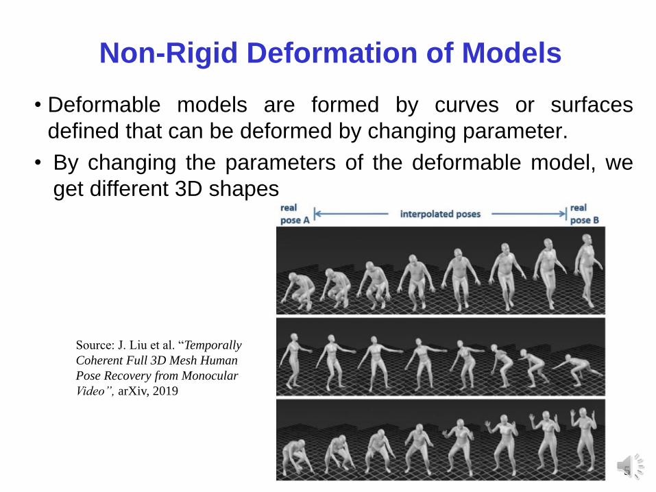
• Deformable models are formed by curves or surfaces
defined that can be deformed by changing parameter.
• By changing the parameters of the deformable model, we
get different 3D shapes
5
Source: J. Liu et al. “Temporally
Coherent Full 3D Mesh Human
Pose Recovery from Monocular
Video”, arXiv, 2019
Computer Generated Models
• Scanning real objects or making deformable models are beyond the
scope of this unit
• We will look into how to generate 3D models using computer software
• We’ll focus only on a couple of fundamental techniques: subdivision
surfaces and animation via skinning.
• Blender
- Blender includes many different tools useful for different kinds of modelling.
- You can import real animations (motion capture) into Blender to animate a
model
6
How can we easily model in 3D?
3D modelling can be tedious and time consuming.
– Even positioning a single point in 3D is tricky – Mice and displays are
2D devices
– OpenGL (and DirectX) is based mostly on drawing many triangles.
– So objects must be constructed from many vertices, edges and faces,
– Placing each vertex/edge/face individually is not usually feasible!
– How can we do this quickly and easily?
7
Can we easily model natural shapes?
We can quickly model “blocky” objects – with only a few faces.
– But most natural shapes aren’t blocky.
We can use prebuilt common shapes like spheres, cylinders, elipsoids,
...
– But these still don’t allow us to create “natural” shapes – most shapes in
the real world aren’t perfect spheres, etc.
– Can we generate shapes with many vertices by controlling just a
few?
8
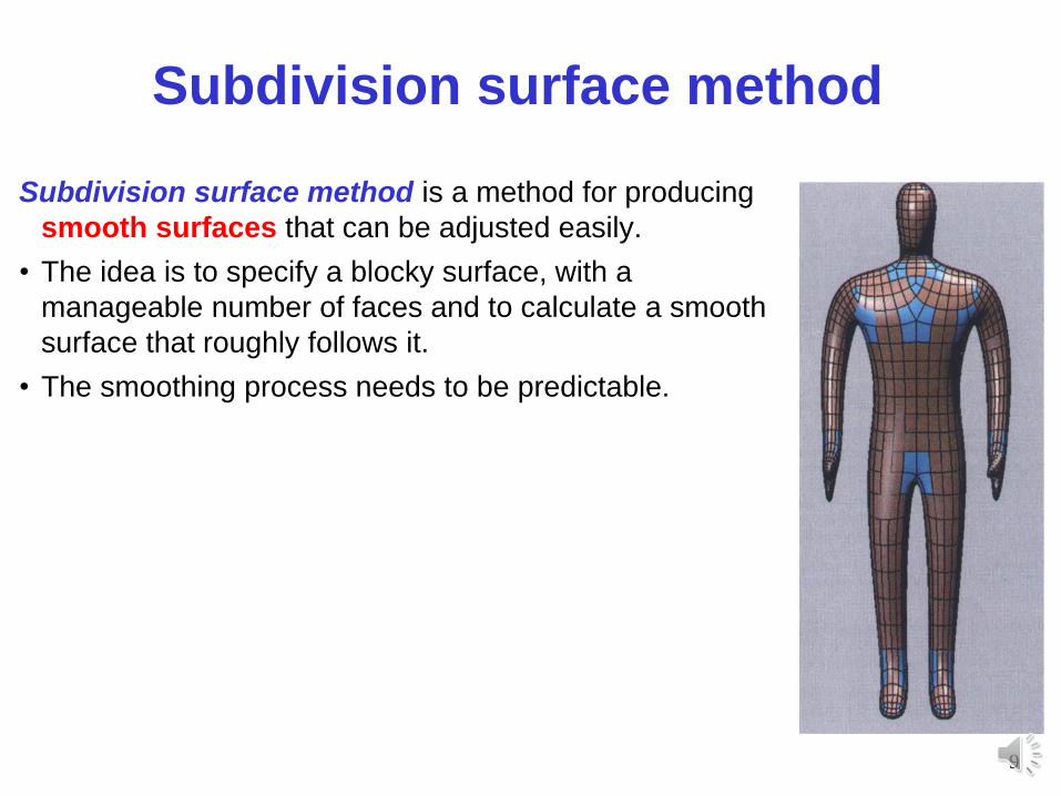
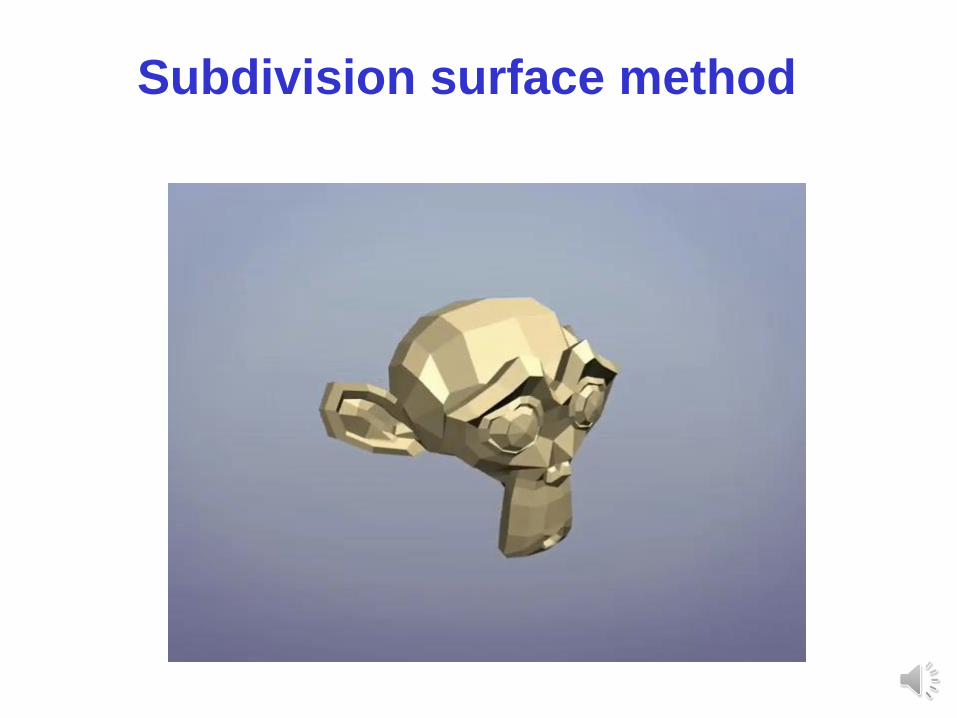
Subdivision surface method
Subdivision surface method is a method for producing
smooth surfaces that can be adjusted easily.
• The idea is to specify a blocky surface, with a
manageable number of faces and to calculate a smooth
surface that roughly follows it.
• The smoothing process needs to be predictable.
9
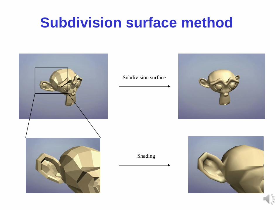
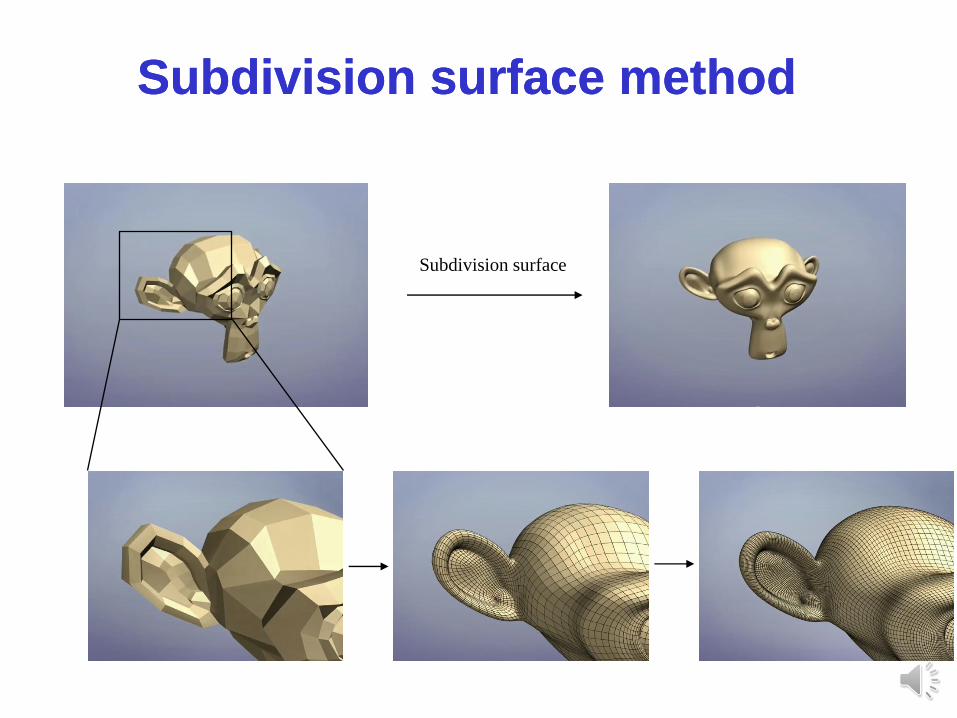
Subdivision surface method
Subdivision surface
Shading
Subdivision surface methodSubdivision surface method
Subdivision surface
Subdivision surface method
Subdivision surface method
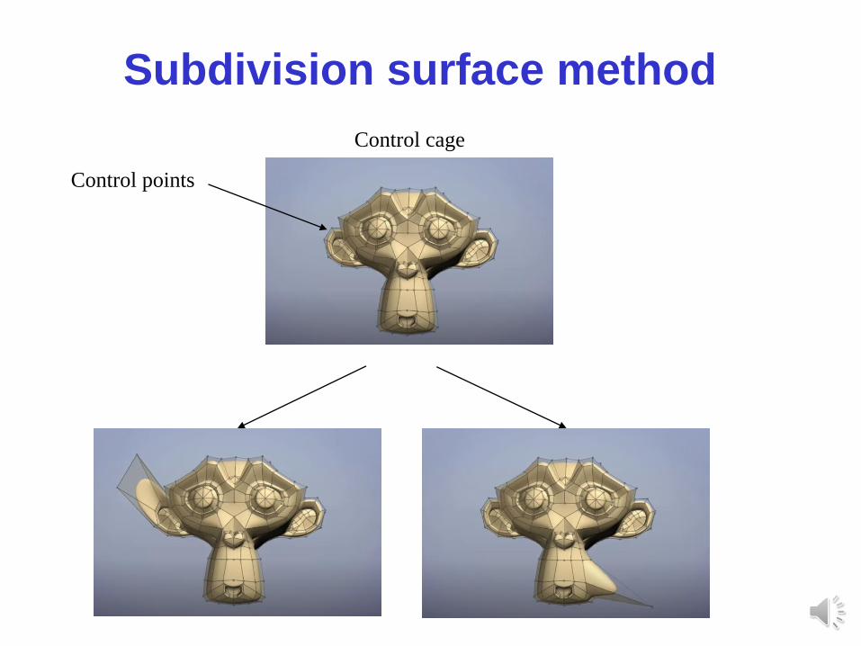
Control cage
Control points
Subdivision surface method
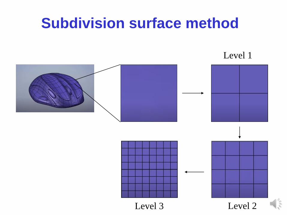
Subdivision surface method
Level 1
Level 2Level 3
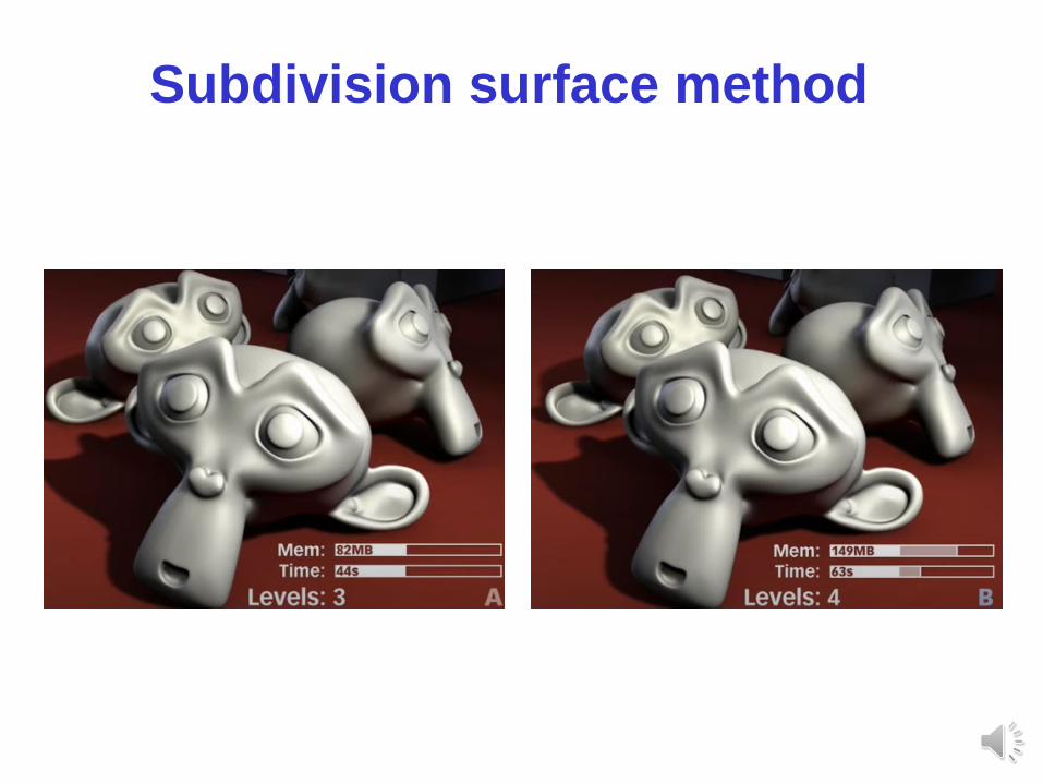
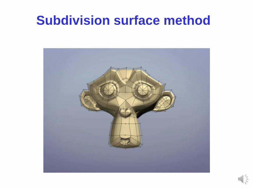
Subdivision surface method
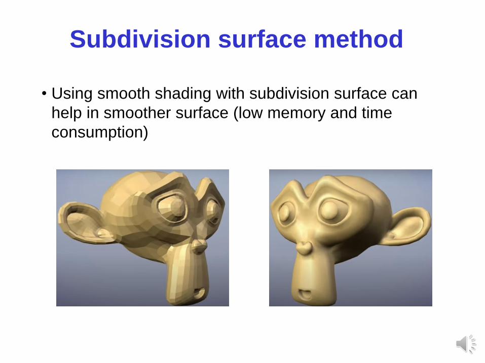
• Using smooth shading with subdivision surface can
help in smoother surface (low memory and time
consumption)
Subdivision surface method
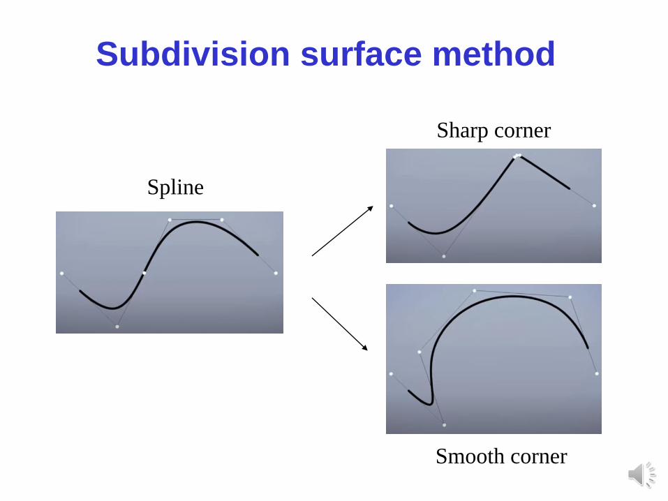
Subdivision surface method
Spline
Sharp corner
Smooth corner
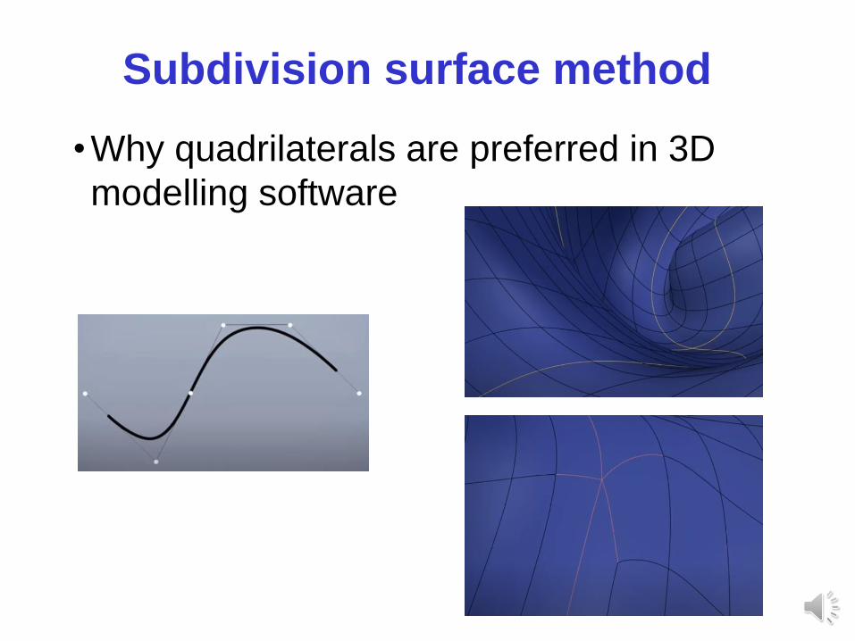
•Why quadrilaterals are preferred in 3D
modelling software
Subdivision surface method
Subdivision surface method
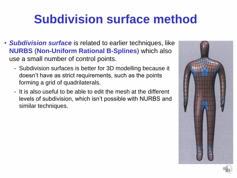
• Subdivision surface is related to earlier techniques, like
NURBS (Non-Uniform Rational B-Splines) which also
use a small number of control points.
- Subdivision surfaces is better for 3D modelling because it
doesn’t have as strict requirements, such as the points
forming a grid of quadrilaterals.
- It is also useful to be able to edit the mesh at the different
levels of subdivision, which isn’t possible with NURBS and
similar techniques.
20
Catmull-Clark subdivision surface
technique
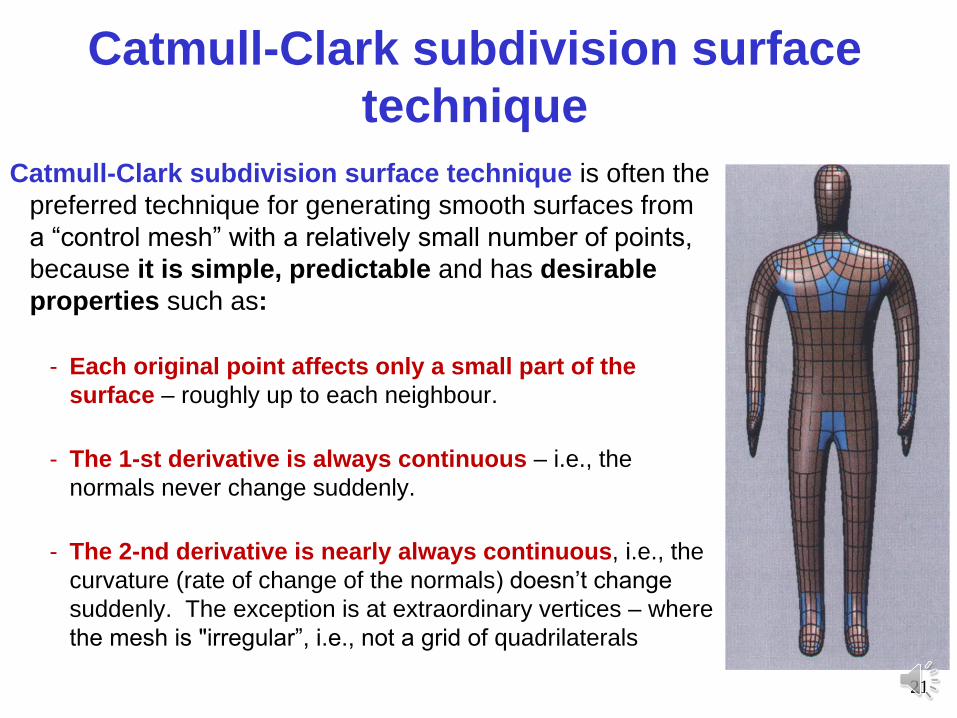
Catmull-Clark subdivision surface technique is often the
preferred technique for generating smooth surfaces from
a “control mesh” with a relatively small number of points,
because it is simple, predictable and has desirable
properties such as:
- Each original point affects only a small part of the
surface – roughly up to each neighbour.
- The 1-st derivative is always continuous – i.e., the
normals never change suddenly.
- The 2-nd derivative is nearly always continuous, i.e., the
curvature (rate of change of the normals) doesn’t change
suddenly. The exception is at extraordinary vertices – where
the mesh is "irregular”, i.e., not a grid of quadrilaterals
21
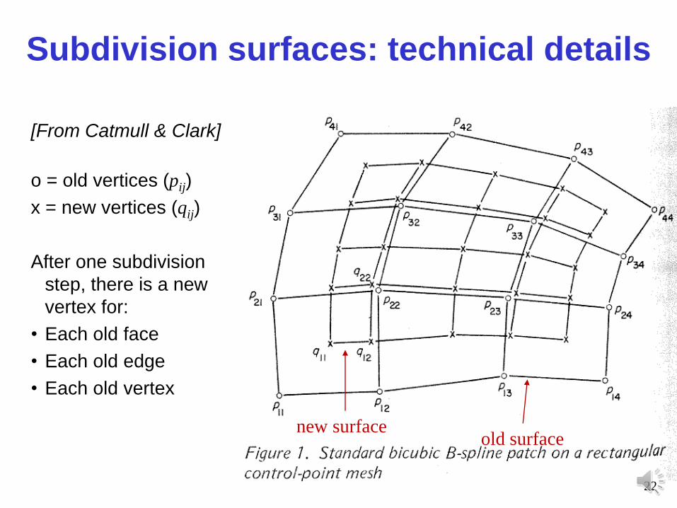
[From Catmull & Clark]
o = old vertices (pij)
x = new vertices (qij)
After one subdivision
step, there is a new
vertex for:
• Each old face
• Each old edge
• Each old vertex
old surfacenew surface
22
Subdivision surfaces: technical details
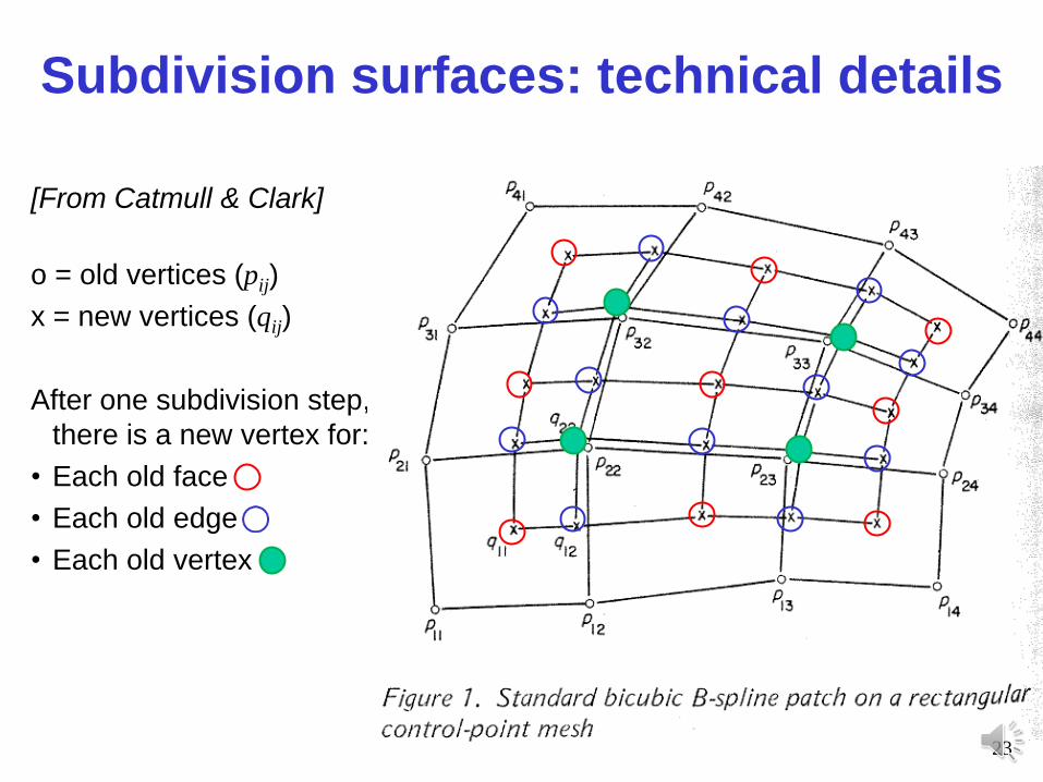
[From Catmull & Clark]
o = old vertices (pij)
x = new vertices (qij)
After one subdivision step,
there is a new vertex for:
• Each old face
• Each old edge
• Each old vertex
23
Subdivision surfaces: technical details
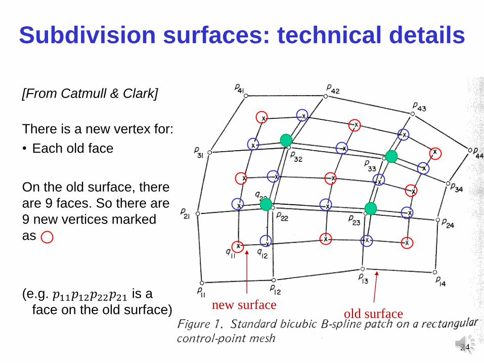
new surfaceold surface
[From Catmull & Clark]
There is a new vertex for:
• Each old face
On the old surface, there
are 9 faces. So there are
9 new vertices marked
as
(e.g. 𝑝11𝑝12𝑝22𝑝21 is a
face on the old surface) new surface
24
Subdivision surfaces: technical details
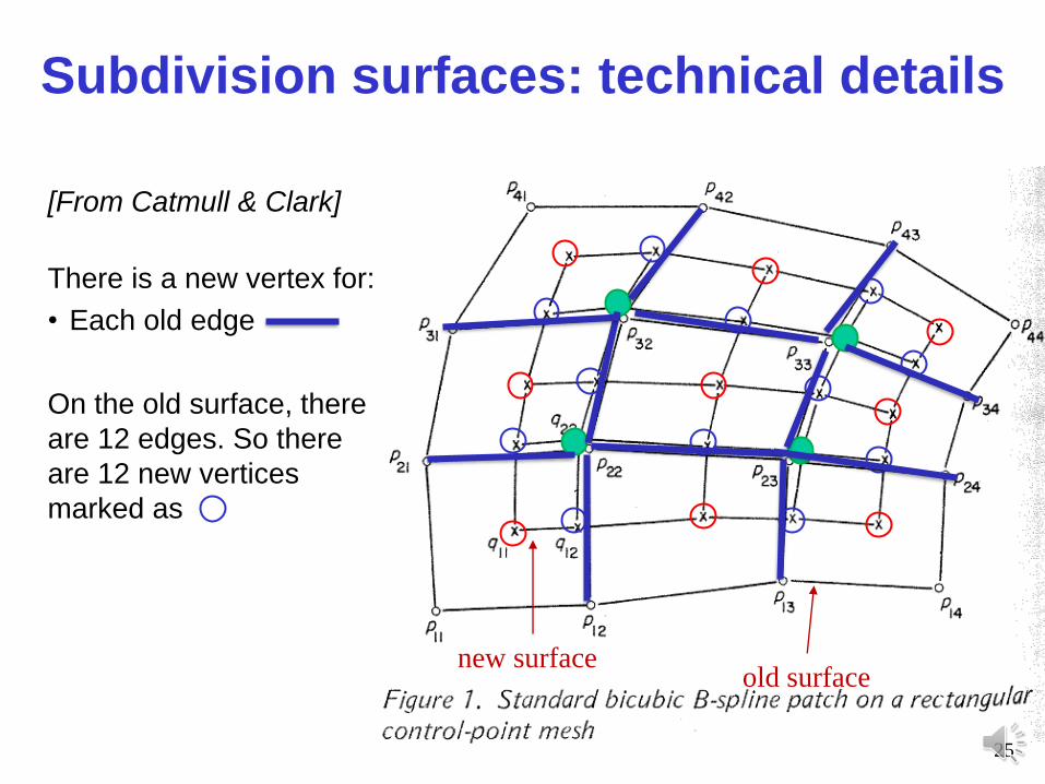
old surfacenew surface
[From Catmull & Clark]
There is a new vertex for:
• Each old edge
On the old surface, there
are 12 edges. So there
are 12 new vertices
marked as
25
Subdivision surfaces: technical details
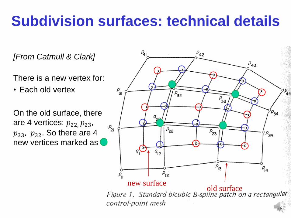
new surfaceold surface
[From Catmull & Clark]
There is a new vertex for:
• Each old vertex
On the old surface, there
are 4 vertices: 𝑝22, 𝑝23,
𝑝33, 𝑝32. So there are 4
new vertices marked as
new surface
26
Subdivision surfaces: technical details
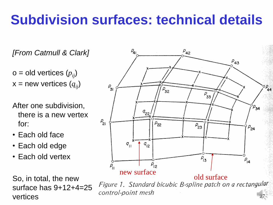
[From Catmull & Clark]
o = old vertices (pij)
x = new vertices (qij)
After one subdivision,
there is a new vertex
for:
• Each old face
• Each old edge
• Each old vertex
So, in total, the new
surface has 9+12+4=25
vertices
old surfacenew surface
27
Subdivision surfaces: technical details
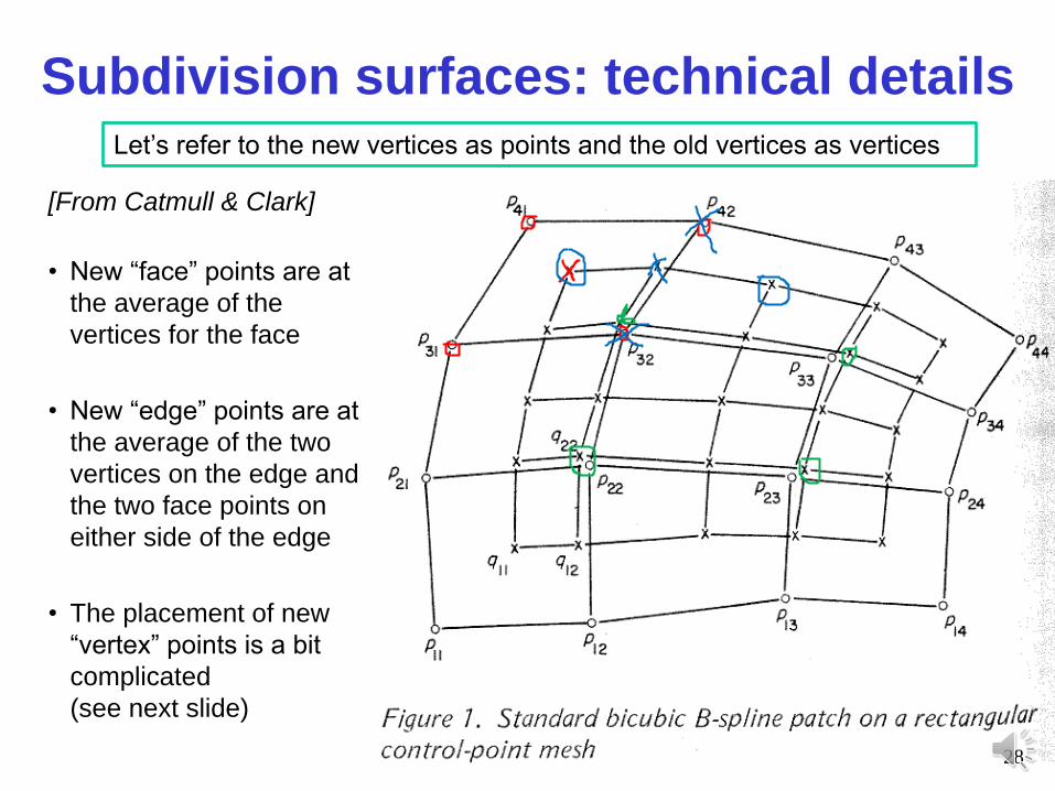
[From Catmull & Clark]
• New “face” points are at
the average of the
vertices for the face
• New “edge” points are at
the average of the two
vertices on the edge and
the two face points on
either side of the edge
• The placement of new
“vertex” points is a bit
complicated
(see next slide)
28
Subdivision surfaces: technical detailsLet’s refer to the new vertices as points and the old vertices as vertices
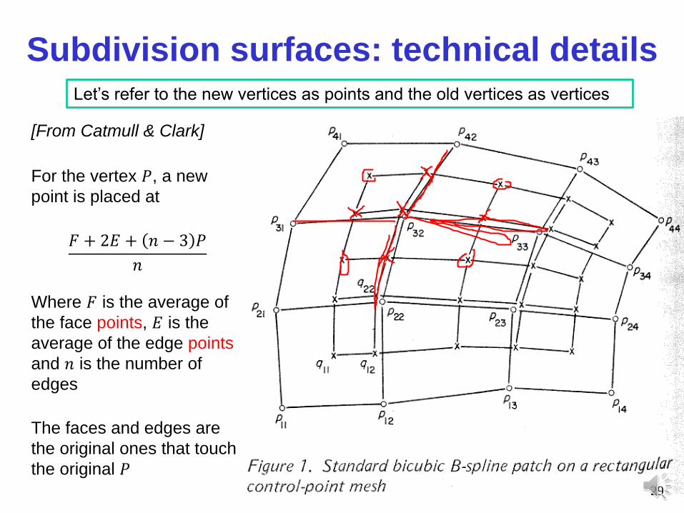
[From Catmull & Clark]
For the vertex 𝑃, a new
point is placed at
𝐹 + 2𝐸 + 𝑛 − 3 𝑃
𝑛
Where 𝐹 is the average of
the face points, 𝐸 is the
average of the edge points
and 𝑛 is the number of
edges
The faces and edges are
the original ones that touch
the original 𝑃29
Subdivision surfaces: technical detailsLet’s refer to the new vertices as points and the old vertices as vertices
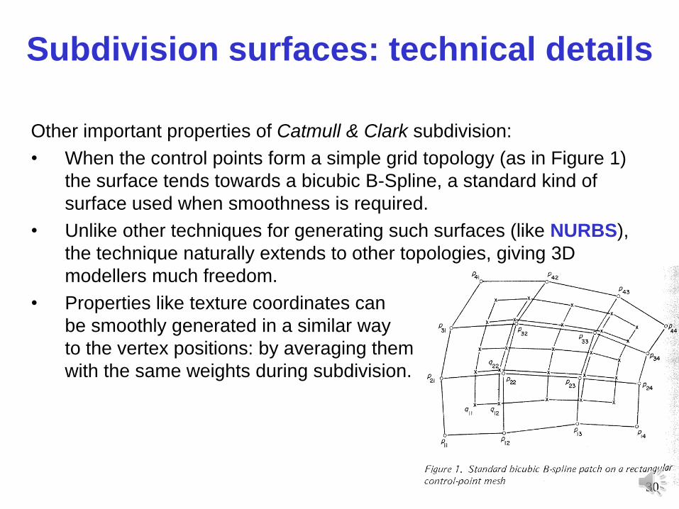
Other important properties of Catmull & Clark subdivision:
• When the control points form a simple grid topology (as in Figure 1)
the surface tends towards a bicubic B-Spline, a standard kind of
surface used when smoothness is required.
• Unlike other techniques for generating such surfaces (like NURBS),
the technique naturally extends to other topologies, giving 3D
modellers much freedom.
• Properties like texture coordinates can
be smoothly generated in a similar way
to the vertex positions: by averaging them
with the same weights during subdivision.
30
Subdivision surfaces: technical details
• Counting the number of new vertices for open surfaces after
one subdivision step can be a bit confusing. For closed
surfaces, the counting is easier and more intuitive.
31
Catmull & Clark subdivision surface method
on closed surfaces
Catmull & Clark subdivision surface method
on closed surfaces
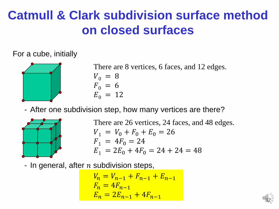
For a cube, initially
- After one subdivision step, how many vertices are there?
- In general, after 𝑛 subdivision steps,
There are 8 vertices, 6 faces, and 12 edges.
𝑉0 = 8𝐹0 = 6𝐸0 = 12
There are 26 vertices, 24 faces, and 48 edges.
𝑉1 = 𝑉0 + 𝐹0 + 𝐸0 = 26𝐹1 = 4𝐹0 = 24𝐸1 = 2𝐸0 + 4𝐹0 = 24 + 24 = 48
𝑉𝑛 = 𝑉𝑛−1 + 𝐹𝑛−1 + 𝐸𝑛−1𝐹𝑛 = 4𝐹𝑛−1𝐸𝑛 = 2𝐸𝑛−1 + 4𝐹𝑛−1
32
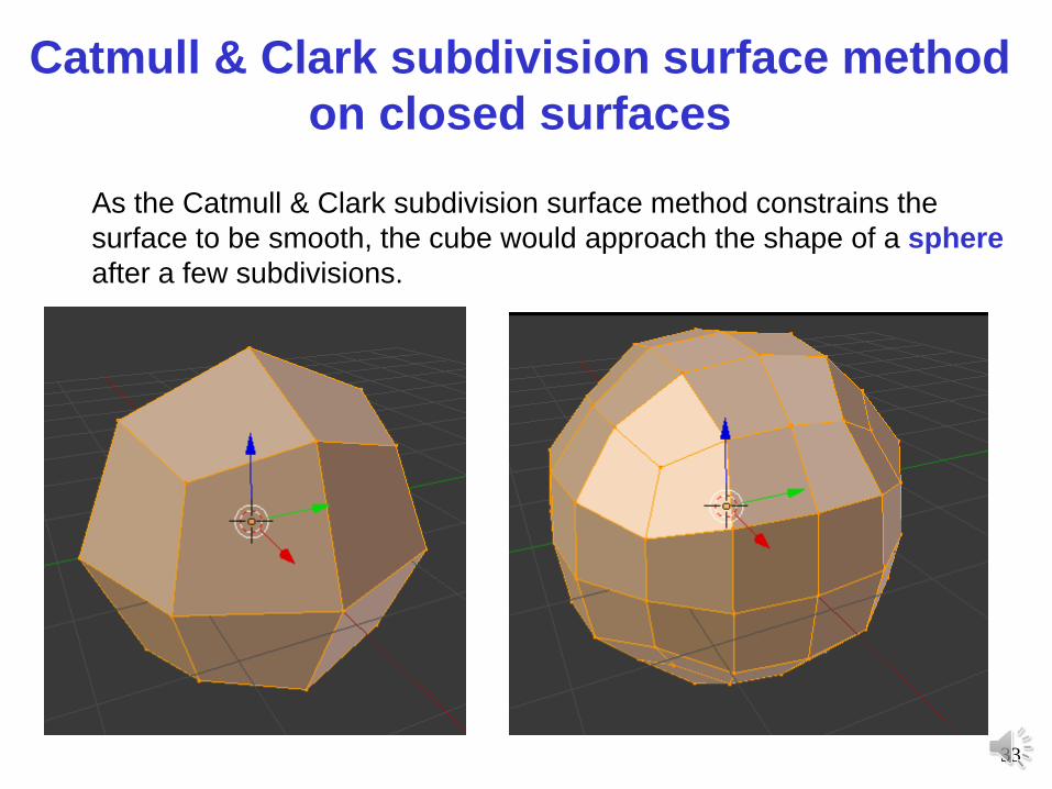
As the Catmull & Clark subdivision surface method constrains the
surface to be smooth, the cube would approach the shape of a sphere
after a few subdivisions.
33
Catmull & Clark subdivision surface method
on closed surfaces
Further Reading
• E. Angel and D. Shreiner: Interactive Computer Graphics 6E © Addison-
Wesley 2012
- Catmull-Clark subdivision Ch-10 Section 10.12
The slides are partially based on “The Guerrila CG Project of guerrilla.org”, topic
Subdivision surfaces: Overview.
34