On the relation between unemployment and housing tenure...
123
UNIVERSITEIT GENT FACULTEIT ECONOMIE EN BEDRIJFSKUNDE ACADEMIEJAAR 2013 – 2014 On the relation between unemployment and housing tenure: the European baby boomer generation Masterproef voorgedragen tot het bekomen van de graad van Master of Science in de Handelswetenschappen Miguel Vandenbussche en Maxime Verhenne onder leiding van Prof. Dr. Carine Smolders
Transcript of On the relation between unemployment and housing tenure...

UNIVERSITEIT GENT
FACULTEIT ECONOMIE EN BEDRIJFSKUNDE
ACADEMIEJAAR 2013 – 2014
On the relation between unemployment and housing tenure: the European baby
boomer generation
Masterproef voorgedragen tot het bekomen van de graad van
Master of Science in de Handelswetenschappen
Miguel Vandenbussche en Maxime Verhenne
onder leiding van
Prof. Dr. Carine Smolders


GHENT UNIVERSITY
FACULTY OF ECONOMICS AND BUSINESS ADMINISTRATION
ACADEMIC YEAR 2013-2014
On the relation between unemployment and housing tenure: the European baby
boomer generation
Thesis presented in fulfillment of the requirements for the degree of
Master of Science in Commercial Sciences
Miguel Vandenbussche and Maxime Verhenne
under the supervision of
Prof. Dr. Carine Smolders


Preface
Ghent, May 2014
We made this thesis as a completion of the Master of Science in Commercial Sciences,
Finance and Risk management at the Faculty of Economics and Business Administration of
Ghent University in the academic year of 2013-2014.
The past year we have been investigating the remarkable relationship between unemployment
and home ownership that was described by a vast amount of academic literature. We wanted
to make a unique contribution to the literature and therefore decided to observe the
relationship for a specific age group that was not yet made, namely the baby boomer
generation. These days, this age group is hot topic for policy makers across Europe as the
baby boomers start to enter retirement age in large numbers.
With help of simple statistical analyses on the data of the SHARE database we were able to
make an academic contribution to the literature. Therefore we would like to thank Josette
Janssen to give us access to the dataset. We must also recognize it is one of the rare large-
scale datasets that is freely retrievable for students.
Furthermore we would also like to thank the people behind the Flemish Policy Research
Centre on Fiscal Policy to supply us with specific information concerning the recent findings
on the subject. Special thanks go to Daan Isebaert and Jan Rouwendal for their presentations
at a study day in Brussels.
Finally, with this preface we would like to underline the gratitude to our promoter, Professor
Carine Smolders, who guided us trough this academic route and gave us the opportunity to
explore this subject profoundly.
Enjoy your reading,
Miguel Vandenbussche and Maxime Verhenne


Acknowledgement
This paper uses data from SHARE wave 4 release 1.1.1, as of March 28th 2013 (DOI:
10.6103/SHARE.w4.111) and SHARE wave 1 and 2 release 2.6.0, as of November 29 2013
(DOI: 10.6103/SHARE.w1.260 and 10.6103/SHARE.w2.260). The SHARE data collection
has been primarily funded by the European Commission through the 5th Framework
Programme (project QLK6-CT-2001-00360 in the thematic programme Quality of Life),
through the 6th Framework Programme (projects SHARE-I3, RII-CT-2006-062193,
COMPARE, CIT5- CT-2005-028857, and SHARELIFE, CIT4-CT-2006-028812) and
through the 7th Framework Programme (SHARE-PREP, N° 211909, SHARE-LEAP, N°
227822 and SHARE M4, N° 261982). Additional funding from the U.S. National Institute on
Aging (U01 AG09740-13S2, P01 AG005842, P01 AG08291, P30 AG12815, R21 AG025169,
Y1-AG-4553-01, IAG BSR06-11 and OGHA 04-064) and the German Ministry of Education
and Research as well as from various national sources is gratefully acknowledged (see
www.share-project.org for a full list of funding institutions).

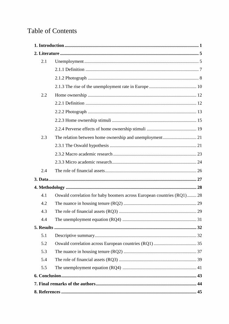
Table of Contents
1. Introduction .................................................................................................................... 1
2. Literature ........................................................................................................................ 5
2.1 Unemployment ................................................................................................... 5
2.1.1 Definition .................................................................................................. 7
2.1.2 Photograph ................................................................................................ 8
2.1.3 The rise of the unemployment rate in Europe ......................................... 10
2.2 Home ownership .............................................................................................. 12
2.2.1 Definition ................................................................................................ 12
2.2.2 Photograph .............................................................................................. 13
2.2.3 Home ownership stimuli ......................................................................... 15
2.2.4 Perverse effects of home ownership stimuli ........................................... 19
2.3 The relation between home ownership and unemployment ............................. 21
2.3.1 The Oswald hypothesis ........................................................................... 21
2.3.2 Macro academic research ........................................................................ 23
2.3.3 Micro academic research ......................................................................... 24
2.4 The role of financial assets ............................................................................... 26
3. Data ................................................................................................................................ 27
4. Methodology ................................................................................................................. 28
4.1 Oswald correlation for baby boomers across European countries (RQ1) ........ 28
4.2 The nuance in housing tenure (RQ2) ............................................................... 29
4.3 The role of financial assets (RQ3) ................................................................... 29
4.4 The unemployment equation (RQ4) ................................................................ 31
5. Results ........................................................................................................................... 32
5.1 Descriptive summary ........................................................................................ 32
5.2 Oswald correlation across European countries (RQ1) ..................................... 35
5.3 The nuance in housing tenure (RQ2) ............................................................... 37
5.4 The role of financial assets (RQ3) ................................................................... 39
5.5 The unemployment equation (RQ4) ................................................................ 41
6. Conclusion ..................................................................................................................... 43
7. Final remarks of the authors ....................................................................................... 44
8. References ..................................................................................................................... 45

Appendix A .............................................................................................................................. 50
Appendix B .............................................................................................................................. 52
Appendix C .............................................................................................................................. 54


1
On the relation between unemployment and housing tenure:
the European baby boomers generation
Abstract
At aggregated level most developed countries are found to have a strong positive correlation between
the rate of unemployment and the rate of home ownership. In academic literature, this phenomenon is
called the Oswald Hypothesis because of Andrew Oswald’s 1996’s pioneering working paper on this
issue. He argued that the rising home ownership rates in OECD countries causes higher rates of
unemployment. As a result of this proposal, a lot of academic work was written that revealed new
insights. In this paper the hypothesis is tested on the so called baby boomer generation (people born
between 1946 and 1964) because, according to academics and policy makers, this specific working age
group bears longer unemployment spells and has a higher probability on being home owner. The
statistical analysis in this paper starts with the correlation for baby boomers across a selection of
European countries that indeed confirms the hypothesis. Later on, the micro level results of this paper
are more nuanced and show that outright owners have a significantly higher chance on being
unemployed and that they are associated with smaller amounts of financial assets in comparison with
mortgagors.
1 Introduction
"There are three kinds of lies: lies, damned lies and statistics." (Mark Twain, 1898)1
This one-line joke is one that many academics and students in economic science ever get
confronted with. Nevertheless, this statement bears an important lesson on the negative
perception for both writers and readers of statistics. On the one hand it is important that
economists and statisticians explain their work at an appropriate level so it can attain
many people. On the other hand it is important that readers are precarious, but try to
understand the point where the human science of economics can meet the exact science of
statistics, so it can be clear how to interpret these statistical results and that readers are for
instance able to apply the correct interpretation of the words ‘correlation’ and ‘causality’.
Essentially, this is what the theory of Oswald is all about. During the 1990s the British
professor - and later on many more academics - found strong correlation between two
macroeconomic fundamentals, which are home ownership and unemployment. The
Oswald hypothesis (Oswald, 1996) states that the growing rate of home ownership in
most developed countries causes higher rates of unemployment. The common sense
explanation argues that living in one’s own house makes people less mobile on labor
markets. Intuitively this is logic, because owners cannot move at the same speed and cost
as renters when looking for a job. One feature that is often investigated in the literature is
the unemployment spell that should – in theory – be longer for home owners compared
with renters, because owners literally ‘stick’ to their homes. In other words, rising home
ownership seems to slowdown the inner mobility at labor markets. But is this really true?
1 Quote retrieved from the autobiography of Mark Twain (Neider, 1959)

2
At a certain moment in time the growing home ownership rate in most OECD countries2
was even mentioned as the missing puzzle part in the economic theory of the natural rate
of unemployment, that was developed in the early sixties of the previous century by
Phelps and Friedman (1968). Nonetheless, this relatively strong correlation does not mean
that - in fact - a casual relation exists between these two macroeconomic indicators.
However, since Oswald presented his rough findings in 1996, a bunch of academic work
followed to unravel the possible mechanisms behind this correlation.
In general, the results across studies are not really consistent. Most of the academic
studies confirm the theory on aggregated data such as in the United States (Green and
Hendershott, 2001) or in Belgium (Isebaert et al, 2013). Since these results suffer from
aggregation bias, more ambiguous research followed on micro data. The results on data
of individuals showed insights for the literature, however they were not really consistent
across time or across countries that could be the result of the fixed-country effects. For
example the Spanish phenomenon in housing culture where obtaining a house for the
children is a family matter (Earley, 2004). Early micro analysis focused on the
unemployment spells of individuals that showed various results. In the U.S.,
unemployment spells were shorter for home owners (Green and Henderschott, 2001) in
contrary to France were this was found to be longer for home owners (Brunet et Lesueur,
2003). Notable is that some concepts became more nuanced, such as the difference of the
effect between an outright home owner and a mortgagor3, and the difference between the
public versus the private renter. A mortgagor for instance has a strong incentive to find a
new job because the mortgage has to be paid off.
Academic literature brings, however, an important problem of the results of Oswald’s
hypothesis that is named endogeneity bias. This problem is typically situated in social and
economic science and can lead to a rejection of a hypothesis that in fact is true.
According to the lectures of Reichstein (2013) the bias can be summarized underlying
two important features. First, omitted variable bias can lead to endogeneity problem such
as described by Van Leuvensteijn and Koning (2004) that certain variables in the model
have limited characteristics that are indeed important for the mechanism. The example
that the authors phrase is job commitment that can explain the housing tenure of people.
This shows that certain variables could be overlooked – or omitted - when explaining
housing tenure or the general unemployment rate model of Oswald. Second, another form
2 The Organization for Economic Co-operation and Development (OECD) current Member countries are:
Australia, Austria, Belgium, Canada, Chile, Czech Republic, Denmark, Estonia, Finland, France, Germany,
Greece, Hungary, Iceland, Ireland, Israel, Italy, Japan, Korea, Luxembourg, Mexico, Netherlands, New
Zealand, Norway, Poland, Portugal, Slovak Republic, Slovenia, Spain, Sweden, Switzerland, Turkey,
United Kingdom, United States 3 In this paper the mortgagor is “the borrower in a mortgage, typically a homeowner” (Oxford dictionary,
2014). The mortgagee however is defined as “the person who is the lender in a mortgage, typically a bank,
building society, or saving and loan association” (Oxford dictionary, 2014)
3
of the endogeneity problem was explained by L’Horty and Sari (2010) which is the
simultaneity bias. It is when variables are determined simultaneously and hence it is not
clear which one evokes the other one. In other words, this reverse causality can be a bias
of the theory because intuitively it is not clear whether someone is (un)employed because
he is a home owner or instead the fact that home ownership makes someone
(un)employed. This paper is however able to work with lagged variables of the tenure
status to address this latter problem. It is a good attempt to solve this problem, but not
completely (Reed, 2013).
Literature does not only link home ownership to unemployment, as there are other
variables that can be influential to both home ownership and unemployment. A possible
suggestion is the role of financial assets, of which less is known in literature. For instance,
Fratantoni (1998) linked housing tenure with the relative weight of investments in risky
assets and found mortgagors to be significantly more risk averse. Financial wealth itself
can also be an incentive to longer unemployment spells as it can be consumed during the
unemployed period (Gruber, 2001). Another relevant finding in this story is that generous
unemployment insurance benefits can undermine labor mobility. Feldstein (1973) for
instance argued that unemployment insurance was responsible for a rise in unemployment
rate. However, he also found that a lot of the benefit receivers were not especially low in
the income distribution. In this optic the Oswald theory may be specifically located with
unemployed (outright) owners who can combine the consumption of financial assets with
the benefits of unemployment insurance during the unemployment spell. That off course
is an incentive for longer unemployment spells.
In this paper the European baby boomer generation is taken into account. The United
States Census Bureau defines this generation as the people that were born in the post-war
housing and education society that started from 1946 and lasted until 1964. The argument
to work with this age group is dual. First, this age group has a significant higher
probability of being home owners in comparison with younger age groups (Andrews and
Caldera Sánchez, 2011). This is relevant, because in developed societies most of their
citizens dream to own their own house one day. In accordance with this dream, it is
plausible that in the year 2011 most of the baby boomers must have achieved their dream,
since the eldest boomers achieved the age of 65, which is the end of working age4. In the
opposite point-of-view, it is logic to perceive the baby boom renters as such that this
tenant choice is either the result of financial restrictions or either a well-thought-out
choice to be flexible in life or work situation and thus not a temporarily situation in order
to still achieve the dream of acquiring one’s own house. This paper’s scope is important
because temporarily housing situations can blur the underlying mechanism(s) of the
4 The SHARE questionnaires were hold in 2011. The oldest baby boomers (born in 1946) achieved the age
65 in the year 2011. (2011 minus 1946 equals 65)
4
theory. Second, it is proved that older workers of 55 years and older have a significant
lower mobility on labor markets because they spend far more time searching for work.
For instance the U.S. average searching period was found to be 56.1 weeks for this age
group in comparison with 35.1 weeks for unemployed at age less than 55 (Rix, 2013).
Thus, these dual finding seems to confirm the Oswald hypothesis across age groups.
Therefore this paper will investigate how strong this correlation really is across European
countries and what the underlying effects may be, such as the role of financial assets.
This paper uses the dataset of the Survey of Health, Ageing and Retirement in Europe
(SHARE) that serves data on European citizens at the age of 50 or more. In the first wave
the data extend to 30,816 observations across twelve countries while seven years later the
database of the fourth wave covers 58,489 individuals over fifteen European countries
plus Israel. In fact only twelve countries are taken into account since the regression
models required appropriate variables and lagged variables are used taken from the
second wave. Nonetheless, these data are ideal because the scope in age fits perfectly with
the age scope of the fourth wave. At the time of the interviews in 2011, the baby boomer
generations was between age 46/47 and age 64/65, which is the eldest age group of the
then labor force.
This papers’ first research question (RQ) checks if the European baby boomer generation
exhibits the correlation on a big dataset (N = 9738) across a selection of European
countries5. This correlation - that is measured with help of an ordinary least squares
(OLS) estimate – is expected to be stronger than Oswald’s original one across the OECD
countries (1997) because of the specific scope in age.
Then, the second RQ applies the nuance of the tenure status that is modeled as dependant
variable by making a sub selection between owners and renters and between outright
owners and mortgagors. In fact, this model tries to predict the probability for each of
these tenure statuses through the effect of unemployment and other control variables such
as gender, education or income. In line with other academic work, it is expected to
observe the incentive of a mortgagor to have a smaller chance on unemployment, because
- intuitively - this person needs to pay off the mortgage and is not willing to lose his or
her house and thus less unemployed.
The third RQ brings up a financial approach to the theory. First a model checks if housing
tenure of the baby boomers effects their choice of holding financial assets. In line with
Frantantoni (1998) it is expected that mortgagors give less weight to risky financial assets
5 The selected countries in the SHARE database for RQ1 are Austria, Belgium, Czech Republic, Denmark,
Estonia, France, Germany, Hungary, Italy, Netherlands, Poland, Portugal, Slovenia, Spain, Sweden and
Switzerland.

5
such as stocks, bonds and mutual funds, in comparison to outright owners.
Eventually, this paper investigates a general unemployment equation in line with Oswald
with help of a logistic model that implies the features of the previous questions, which are
the nuance of the housing tenure, financial assets, weight of risky assets in the financial
portfolio.
The second section offers a brief view on the literature that pursued Oswald’s (1996) up
to now, but the section is initiated with a photograph on the indicators ‘unemployment’
and ‘home ownership’, joined with an academic approach on these two macroeconomic
indicators. The third and fourth section incorporates the investigated data with the chosen
methodology. Eventually the results of this methods are shown in section five, just before
the conclusion in the sixth section. Finally, the paper is extended with a discussion for
future research.
2 Literature
2.1 Unemployment
“Unemployment insurance is a pre-paid vacation for freeloaders” (Ronald Reagan, 1966)
The era of Ronald Reagan is often described as ‘neoliberal’ and is in the optic of
oversimplified one-liners probably not different from other eras. The former Governor of
California depicts unemployment as a comfortable position because his statement builds a
bridge between the pleasant thought of vacation and the choice to be unemployed. In fact,
when Reagan became President of the U.S. in 1981 the unemployment rate was rising to
very high levels as a result of the lasting recession due to the oil crisis of 1973. When the
rollercoaster of the business cycle is speeding downwards, workers do not have much of a
voluntary choice when employers - en masse - go astray. Besides, academics have
pointed to the bitter fruits of joblessness. It is proved that being unemployed is a form of
distress that statistically bears significantly higher suicide rates, especially for men, since
the risk of suicide death in e.g. England and Wales (Charlton et al., 1992) was found to be
three times greater than average. Other results from the United Kingdom by Platt and
Kreitman (1985) even found a twelve time greater than average chance of attempting
suicide for long term unemployed Brits. An even more remarkable finding is Oswald’s
(1997) who observed that the rising suicide rate in Western countries since the 1970s
moves along with the rising unemployment rates. (Oswald, 1997).
However, a change of heart for this first – skeptical – paragraph may be found with the

6
time frame. Into the late 1970s, the Federal Reserve6 had a hard time making choices
between unemployment and inflation. Theory and practice used to show a strong trade-off
between these two macroeconomic indicators, that was named the Phillips curve. But by
the beginning of the decade the effect seemed to be gone for good due to the rational
expectations of workers and unions who claimed wages, that could capture the expected
inflation. As a result, the reality in the 1970s showed both high unemployment and high
inflation. This devastating finding on the Phillips curve came by Phelps and Friedman
(1968), Lucas (1976) and others. It’s because of these observations that the policy
performed under ‘the Reagan Administration’ had to make choices in order to drop the
high unemployment rates7 from the early 1980s. The chosen policy was – similar to the
introducing quote – quite harsh. It incorporated a decline in minimum wages, a full
taxation of unemployment insurance and work requirement for the unemployed.
Nonetheless, it was very successful as the unemployment rate dropped to its natural level
at the end of his Presidency8. His chief economic advisor even stated: “It was very
successful, especially in comparison with Europe, where the unemployment protection
policies led to double digit unemployment rates.” (Feldstein, 1997). Despite, critics argue
that this pride statement is questionable because the fundamental reason for change of the
economic climate and that of unemployment is not per se due to the chosen policy but
rather to the underlying business cycle that moves up and down every now and then and
is merely based on the monetary policy. (Krugman, 1982). In line with this critique,
recent work of Drehmann et al. (2012) reminds us to the financial cycle that is very
influential – more precisely procyclical - to this business cycle (see figure 1). In fact, the
financial cycle tracks the level of credit and property prices and moves along in intervals
of about sixteen years which is twice as slow as the business cycle. According to the
authors’ observations, the beginning of the 1980s showed a very strong upward trend for
this financial cycle that probably is due to the effect of financial liberalization. So it is
doubtful whether specific unemployment policies had such a great effect on lowering the
unemployment level. It seems rather the effect of bigger phenomena. Yet, less is known
about these real drivers such as the financial cycle.
6 The Federal Reserve is the central banking system of the United States that has mandate on the U.S.
monetary policy. (Meltzer, 2010) 7 According to the statistics of the United States Department of Labor, the rate of unemployment reached
9.7% in 1982. (U.S. Department of Labor, 2014) 8 The unemployment rate in 1988 was 5.5%. (U.S. Department of Labor, 2014)
7
Figure 1: The financial and business cycles in the United States (Drehman et al.,
2012)
Returning back to unemployment on individual level, financial incentives are at work as
well. A working paper of Tatsiramos (2006) argues that an unemployment insurance
reduces the incentive for leaving unemployment. When comparing the diverse
unemployment insurance systems across Europe it is clear that more generous systems
lead to longer periods of unemployment for individual unemployed persons. The writer’s
diagnose is that welfare countries in Europe have taken away the incentive to work.
Hence, it is notable that the phenomenon of unemployment is not easy to understand and
that analyzing, debating, avoiding this phenomenon should happen with an appropriate
level of distinction. For instance the distinction between structural and cyclical
unemployment that was discussed in the previous paragraph. Besides, this can be for
instance very country specific, such as the well known and unique example of Denmark.
The country is perceived as a “flexicurity” welfare state because it has a highly flexible
labor market with high mobility and a high employment rate in combination with good
protection mechanisms for workers, such as high minimum wages and long generous
unemployment insurances (Andersen, Svarer, 2007). As it is notable, these country-
specific incentives must be distinct when analyzing this macroeconomic indicator.
2.1.1 Definition
Unemployment seems easy to understand, but it in fact it’s not. Observing unemployment
rates in reports, papers or policy programs may be misleading because definitions of the
concept can vary. Briefly, two categories of definitions can be observed
First, in sensu stricto, the most known and applied definition of unemployment is the one
used for the harmonized unemployment rates in OECD countries. The applied definition

8
is based on the International Labor Organization (ILO) that defines unemployment as “a
person - at working age who - in a certain reference period is:
without work, that is, were not in paid employment or self employment during
the reference period;
currently available for work, that is, were available for paid employment or
self-employment during the reference period; and
seeking work, that is, had taken specific steps in a specified recent period to
seek paid employment or self-employment. “(ILO Conference of Labour
Statisticians, October 1982)
Second, in sensu lato, broader definitions of being unemployed are found. In line with the
application of the critique of Brandolini et al. (2004) the unemployed can be divided into
four groups:
i. persons who do not want a job
ii. persons who are not searching but might take a job if offered,
iii. persons who are looking for a job and took specific steps in the last four weeks
(this is similar as the definition of the ILO)
iv. and finally persons who are searching for a job but took their last step more
than four weeks before the observation moment.
The ILO standard only incorporates category three and defines the other categories as
inactive people. According to Brandolini et al. (2004) it is because of the negligence of
category four that approximately one fifth of the European unemployed during the 1990s
was left out of the unemployment statistics. The reason is that the arbitrary chosen four
week period does not capture this group. In fact, this was revealed during the 1990s by
the Italian Statistics Agency (Istat) that did not apply this ‘four weeks’ rule. (Brandolini et
al, 2004). Notable is that the author suggests that the best distinction for the definition is
to check whether an unemployed person is really looking for a job or not. Besides, one
can also argue whether category two or even one concerns unemployed persons, as being
long term unemployed can be demotivating for the individual.
2.1.2 Photograph
Europe’s unemployment rates are heterogeneous (see table 1). With the help from the
Organization for Economic Co-operation and Development (OECD) statistics, this
section presents a brief picture of the 2011 harmonized unemployment rates and its
evolution (see figure 2) between 1990 and 2010 for all age groups.
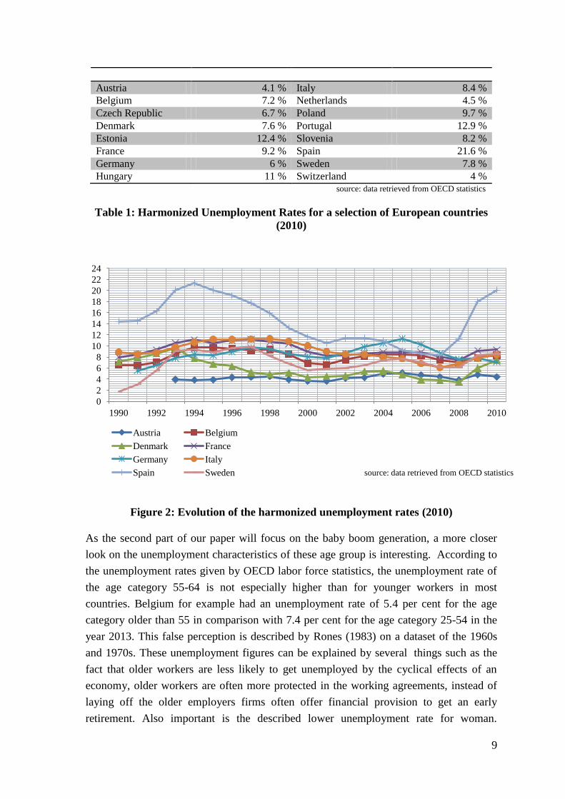
9
Austria 4.1 % Italy 8.4 %
Belgium 7.2 % Netherlands 4.5 %
Czech Republic 6.7 % Poland 9.7 %
Denmark 7.6 % Portugal 12.9 %
Estonia 12.4 % Slovenia 8.2 %
France 9.2 % Spain 21.6 %
Germany 6 % Sweden 7.8 %
Hungary 11 % Switzerland 4 %
source: data retrieved from OECD statistics
Table 1: Harmonized Unemployment Rates for a selection of European countries
(2010)
Figure 2: Evolution of the harmonized unemployment rates (2010)
As the second part of our paper will focus on the baby boom generation, a more closer
look on the unemployment characteristics of these age group is interesting. According to
the unemployment rates given by OECD labor force statistics, the unemployment rate of
the age category 55-64 is not especially higher than for younger workers in most
countries. Belgium for example had an unemployment rate of 5.4 per cent for the age
category older than 55 in comparison with 7.4 per cent for the age category 25-54 in the
year 2013. This false perception is described by Rones (1983) on a dataset of the 1960s
and 1970s. These unemployment figures can be explained by several things such as the
fact that older workers are less likely to get unemployed by the cyclical effects of an
economy, older workers are often more protected in the working agreements, instead of
laying off the older employers firms often offer financial provision to get an early
retirement. Also important is the described lower unemployment rate for woman.
0
2
4
6
8
10
12
14
16
18
20
22
24
1990 1992 1994 1996 1998 2000 2002 2004 2006 2008 2010
source: data retrieved from OECD statistics
Austria Belgium
Denmark France
Germany Italy
Spain Sweden

10
Especially in older data it is acceptable that older woman have lower unemployment rates
as they withdraw from the labor market more often because of lack of the career-
orientation (Rones, 1983). It is however proved that older workers generally have a
significant lower mobility on labor markets because they spend far more time searching
for work. For instance the U.S. average searching period was found to be 56.1 weeks for
this age group in comparison with 35.1 weeks for unemployed at age less than 55 (Rix,
2013). So this false perception of older workers is in fact true but only in case of the
unemployment spell and thus not in the unemployment rate.
2.1.3 The rise of the unemployment rate in Europe
Figure 3: The unemployment rate for EU-15 (Blanchard, 2006)
Literature is clear. Most of the European countries have seen unemployment rates
growing since the 1970s. The above figure by Blanchard (2006) - retrieved from the
OECD database – shows a significant growth of the relative share of unemployed
Europeans9 across the past decades. Moreover, the fluctuations of the unemployment rate
seems to be more volatile as it moves with the business cycle. (Blanchard, 2006) This is a
remarkably finding because during the same period the U.S. unemployment rate didn’t
show such a trend at all. In fact, the U.S. unemployment rate was quite stable over time
and before the 1970s it was consistently higher than the European rates. (Blanchard,
2006). According to Solow, the most remarkably about the European rate is that it
dominates the business cycle. (Solow, 2000) This means that the growing part of
unemployment is rather structural and less a result of recessions in the business cycle
9 The EU-15 countries are: Austria, Belgium, Denmark, Finland, France, Germany,
Greece, Ireland, Italy, Luxembourg, Netherlands, Portugal, Spain, Sweden and United
Kingdom

11
rollercoaster.
So, what is this theory of the natural rate of unemployment all about? Today, most
macroeconomic course books threat this concept, that was initially formulated in the
1960s by two economists named Milton Friedman and Edmund Phelps. The formulation
was in fact very simple: “an economy will have a sort of constant rate of unemployment
that is rather structural because it is evoked by factors such as labor market imperfections,
costs of information, deceleration or non access to vacancy information and costs of
mobility” (Friedman, 1968). This statement was based on the perception of looking at
labor markets through the eyes of equilibrium models, the so called Walrasian systems.
As the professor argued, it is important to note that this rate depends on the policy of the
nation or of a central bank and, as a result of this, is not per se unchangeable over time.
Therefore, many teachers and writers need to note that the word ‘natural’ of the theory of
the natural rate of unemployment is rather confusing because it – as for example the
European rate - moves over time.
According to Blanchard and Katz (1996), the past research between the 1970s and the
1990s on the potential explanations of this rising unemployment rate are various and
rather unreliable because unrevealing this puzzle was neither consistent across time, nor
across countries. The potential determinants that were presented by academics over these
years drove from the increase of price of energy, the slowdown of productivity growth
(Bruno and Sachs, 1985), the impact of taxes on wages (Bean et al., 1986), loss of skills
due to long term unemployment (Blanchard, 1991), labor market rigidities such as the
firm’s cost and term of firing workers (OECD Jobs Study, 1994) or either the growth of
unskilled workers due to fast technological progress (Krugman, 1994). One can off course
argue about the country specific differences, but the utter diagnose, which Blanchard and
Katz mentioned in 1996 at the bottom line of their paper is the discrepancy between
macroeconomic view on the natural rate of unemployment and the micro economic
findings by labor economics. Or to use their words: “We thus end with a plea for more
joint efforts by macro and labor economists to better integrate theoretical and empirical
work on wage determination and unemployment.”
Later on, it was Flatau et al (2003) who first related the Oswald hypothesis as a possible
explanation of the rise in the natural rate of unemployment for the observed OECD
countries. The hypothesis is that the rising rate of home ownership since the second world
war is not strictly due to labor-market characteristics, but a possible consequence of the
growing home ownership rate in most developed countries.
12
2.2 Home ownership
“Deep in the hearts of most American families glows, however faintly, the spark of desire
for home ownership.” (U.S. Department of Commerce, 1942)
Owning your own house is one of the main purposes in life for most of us and is an
important part of the American Dream. The benefits of owning your own house are
enormous: it stabilizes communities and leads to more responsibility for the living
environment (diPasquale, Glaeser, 1999), houses look greater because the owner has a
strong incentive to maintain them (Coulson, 2002) and it has a positive effect to personal
satisfaction and self-esteem (Rohe, Stegman, 1994).
However, recent events - such as the U.S. housing bubble burst of 2007 - showed that the
benefits of this dream doesn’t always follow reality. This is an indication that policy
makers need to be thoughtful when implementing this part of the American Dream. Also
other perverse effects can be part of the double edged sword of home ownership.
2.2.1 Definition
Literature defines home owners as owner-occupiers: “a housing unit is owner-occupied if
the owner or co-owner lives in the unit, even if it is mortgaged or not fully paid for.” (U.
S. Census Bureau). This means for example that someone who owns a house but lives in a
rental apartment is no longer perceived as a home owner, but instead as a tenant.
However, according to Proxenos (2002) there is no strict definition of home ownership
itself. The interpretation of home ownership differs from one country to the next. Where
one country considers a mobile home as ownership, another country would not. Also the
definition of home ownership tells nothing about the quality of the owner-occupied
houses. This can lead to an over-estimation bias between the home ownership in countries
especially at a global scale. This means that in some cases it is not justified to compare
these rates as they are not based on the same funding definitions, this estimation can lead
to misleading results. Besides, it is also possible that a bias appears in surveys when the
concept of home ownership is not well defined to the respondents.
13
Since the 1990s, organizations such as the OECD and Eurostat started tracking the rates
of home owners of nations in order to benchmark. These percentages represent the sum of
dwellings that are owned outright or purchased with a mortgage in relation to the total
dwelling stock. This latter incorporates the total of home owners plus tenants. (European
Mortgage Federation, 2004). Thus, the rate is equated as follows:
2.2.2 Photograph: ownership rate
When investigating these ownership rates, two facts are consistent across academic
research. First, on a long time horizon nearly all countries experienced a growth of the
share of home owners. Second, these ownership rates strongly differ across countries
(Andrews and Caldera Sanchez, 2011). The overall average home ownership rate once
was measured across 106 countries on data from the World Bank and it was found 67.8
per cent with a median of 69.3 per cent. (Fisher and Jaffe, 2003). For a selection of
OECD countries, Andrews and Caldera Sanchez (2011) describe this evolution and build
models to decompose its determinants. However, the they strongly differ. For example in
2004 Spain had an ownership rate of 83.2 per cent while Switzerland’s did not even
reached half this percentage with 38.4 per cent.
A more nuanced way of observing the housing tenure of citizens is the distinction
between private or public renter and the distinction between a mortgagor or a household
that has no outright owner as this was confirmed recently by researchers such as Nijkamp
and Rouwendal (2007). The EU Statistics on Income and Living Conditions (EU-SILC)
survey measures a range of structural indicators of living conditions. One is the tenure
status of the individual households. (see Figure 4) A few substantial differences between
the member states arise. Northern countries as Denmark, Netherlands, Sweden and also
Switzerland have very little outright owners, but instead a very substantial share of
mortgagors. Also countries such as Germany, Austria and Switzerland have
proportionally a high share of renters compared to the other countries. For instance the
share of Swiss tenants is almost 60 per cent.

14
Figure 4: Housing tenure in Europe (2010)
When investigating the determinants of these heterogeneous rates, some predictive power
was found for the effect of housing credit. (Fisher and Jaffe, 2003) Most countries’
policies offer a contribution scheme for housing finance. However, a single equation
model for explaining the traditional economic determinants of home ownership rate
across countries was not consistent. The country specific differences on cultural, law,
economic or political fields seems to be too harsh to make a generalized econometric
model with consistent results. It seems that incentives for ownership are very diverse
across countries.
Although there is perception that home ownership is linked to the wealth and strength of
an economy, such as suggested in the American dream, the adverse is proved by the
poorer European countries where ownership rates are very high, such as Greece and Spain
(Earley, 2004). This could for instance be caused by the cultural differences between the
more northern and the southern European countries. This is explained by the fact that in
southern societies have strong traditions of the family being involved in the
accommodation choices of their children. An example of this is the proportion of children
living at home that was found the highest in these southern countries (Earley, 2004). This
means that children stay longer with their parents so that they have a better financial
support when eventually leaving the family home. It seems logic that this phenomenon
leads to lower demand of rental units in these states. And thus the rental market is
underdeveloped.
0%
20%
40%
60%
80%
100%
Owner, no outstanding mortgage or housing loan (=outright owner) Owner, with mortgage or loan (mortgagee) Tenant, rent at market price Tenant, rent at reduced price or free
source: data retrieved from Eurostat, based on EU-SILC

15
Also remarkable are the Eastern European countries that have very high ownership rates
as a result of the communist legacy. During the communistic era it was the state that
owned a large share of the housing system. These housing units were part of cooperatives
during the 1980s. After the fall of communism in 1989, most of the countries experienced
a wave of privatization of ownership. As a result homes were offered for free to its
inhabitants and almost every ex-communistic country developed these remarkable high
rates of home ownership (Struyk, 2000).
2.2.3 Home Ownership Stimuli
“When it comes to economics people have emotions, it's not like chemistry or physics”
(Shiller, 2013)
These days, the most persistent feature to promote home ownership seems to be the home
mortgage interest deduction (HMID) systems in fiscal policies. This system gained a lot
of popularity among tax payers, since they are able to reduce their fiscal expenses.
However, another pallet of less known or less rational stimuli for home ownership exists.
Irrationality and herd behavior
As houses are often seen as an important asset investment, it may be interesting to
perceive decision making stimuli with a financial approach. Let’s start with two of the
three 2013 Nobel Prize winners in Economic Science, Robert Shiller and Eugene Fama.
Something strange appears in their financial theories. These academics totally disagree.
The 1970s were - concerning financial theories - the golden decade for the “efficient
markets” theory. Fama said that capital markets were “efficient”. This is the case when
investors of capital products act completely rational because their decisions to buy or sell
are based on all available information at the moment of their transaction. Fama argued
that all available information is thus reflected in the price of this asset (Fama, 1970).
Contrary, Shiller began talking about behavior finance and argued that people do not
always behave rationally. Examples come from social science and are for instance
wishful thinking or herd behavior. These features eventually can evoke so called
“irrational exuberance” in financial markets (Shiller, 2000), but also in housing markets
(Shiller, 1989). It was in this optic that Case and Shiller warned for a housing bubble on
the U.S. housing market in 2004 (Shiller and Case, 2003). According to the researchers
housing prices could no longer solely be explained by fundamentals such as population
growth, construction costs, income growth or tax rates. Their arguments were also based
on qualitative evidence that showed homebuyers’ perception of buying a house more and
more as a result of making an investment. Also, their survey showed that a major
motivation of buying a home was the expected future appreciation of the house price.
More than 90 per cent of the respondents expected an increase in home prices in the next

16
seven years. However, in reality, the U.S. housing bubble collapsed in 2007 with negative
corrections of 30 per cent10
and more resulting in prices far beneath these expectations.
So it seems that one of the incentives to buy a house can come from herd behavior and
also can be explained by irrational expectations. Briefly, these stimulus seems to be the
result from mythical expressions such as “land is scarce, prices can only rise” that should
better be replaced by “what goes up, may come down”.
Home ownership programs
Underneath this irrational expectations may lie a certain governmental policy that evoked
this. One of the systems that led to a lot of attention because it was pointed as one of the
causes of the U.S. housing bubble in 2007 is the policy that President Clinton started in
the U.S. under the name of the National Home ownership Strategy. The president defends
his policy on stimulating ownership based on its social and economic benefits:
“Home ownership encourages savings and investment. When a family buys a
home, the ripple effect is enormous. It means new home owner consumers. They
need more durable goods, like washers and dryers, refrigerators and water
heaters. And if more families could buy new homes or older homes, more
hammers will be pounding, more saws will be buzzing. Homebuilders and home
fixers will be put to work. When we boost the number of home owners in our
country, we strengthen our economy, create jobs, build up the middle class, and
build better citizens.” (Clinton, 1995)
Before the 1960s, policies facilitating home ownership were initially established to
encourage other purposes such as to boost economy out of recessions. But by the time
such a measure was eventually operational, the actual recession was already gone.
However, as these measures were enacted they had a significant impact on housing on the
long run. (Carliner, 1998) The reason why it had grown is merely due to the overall
economic growth and lower interest rates than to any specific housing policies.
Under the Clinton Administration the home ownership rate – as measured by the U.S.
Census Bureau – rose to 68 per cent by the end of 2001. (Bratt, 2002). Next came the
American Dream Down Payment Assistance Act under the Bush administration, that had
a specific target group (Bush, 2003). A budget of 200 million dollars was provided by the
government to support low income families.11
This law and many others which aimed to
create a society of home owners eventually lead to an increase of the ownership rate to a
10
According to the Case-Shiller Home Price Index (2014)

17
record height of 69.4 percent in June 2004, according to the United States Census Bureau.
Beside these programs, other aspect of pro-home ownership policies can declare the rise
of home ownership within the U.S., namely the innovations in the mortgage financing
business and the flexibility in repayment schedules (Doms and Motika, 2006). A good
example of these innovations are Fannie Mae and Freddy Mac, which are the most known
government-sponsored mortgage enterprises that had a big impact in the mortgage
financing industry as their activities raised significantly from the 1990s tot the early
2000s (Roll, 2002). During this period they contributed to the creation of the so called
‘mortgage backed securities’ (MBS) that ignored the real credit worthiness of the
individual mortgagors, and was able to pass – or secure – the risk to the financial markets.
(Diamand and Rajan, 2009).
Home Mortgage Interest Deduction (HMID)
Most of the industrialized countries handle a fiscal policy program to offer their citizens
an incentive to buy a house. The ideology in the eyes of policymakers is that private
home ownership has many benefits for society as a whole. The applied systems across
most European nations are very similar and incorporates an income tax deduction of the
interests that are charged on the outstanding mortgage linked to the property that the
owner is acquiring. This means that governments are stimulating people to take a loan for
financing one’s own house.
As mentioned by Oswald (1999) Spain and Switzerland are two very contrary cases
within European home ownership statistics. In Switzerland, the authorities do not
promote housing on national level to increase the home ownership rate. This is reflected
in the less favorable fiscal tax systems for home owners. Although interest of a mortgage
is tax deductible, it is rather low because many taxes are added. A property tax also is
added to the taxable income, which is similar to rental income. Besides, when a house is
sold a tax performs on the capital gain. (Kirchgässner, Pommerehne, 1996) This policy
can be explained by the fact that around two-thirds of the Swiss households are renters. A
characteristic of this developed rental market are the institutional investors who own more
than one fourth of this market. (Bourassa et al., 2010) The contrary is seen in Spain where
the authorities promoted home ownership for a long time. However, since the March
2012 – as a result of the economic crises and the Spanish housing bubble – interests on
mortgages and capital payment are no longer tax deductible (PWC, 2012). It will be
interesting to see what impact this measure has on the home ownership rate in the
upcoming years.
Besides, it is also questionable whether these policy measures really are (or were)
18
effective. As told by Glaeser and Shapiro (2002) these home ownership policies mainly
aided the wealthier owners instead of following the ‘American dream’ philosophy where
it is for everyone to obtain a house. Evaluating the different mortgage deduction policies
over the years the real effect on the rate of home ownership is minimal, as it has mainly
influenced the housing consumption and as a result missed its original purpose. Glaeser
and Shapiro argue that the best evidence is the fact that the U.S. ownership rate did not
augment significantly over the past 40 years although the existence of a mortgage interest
deduction has gained much of popularity among owners.
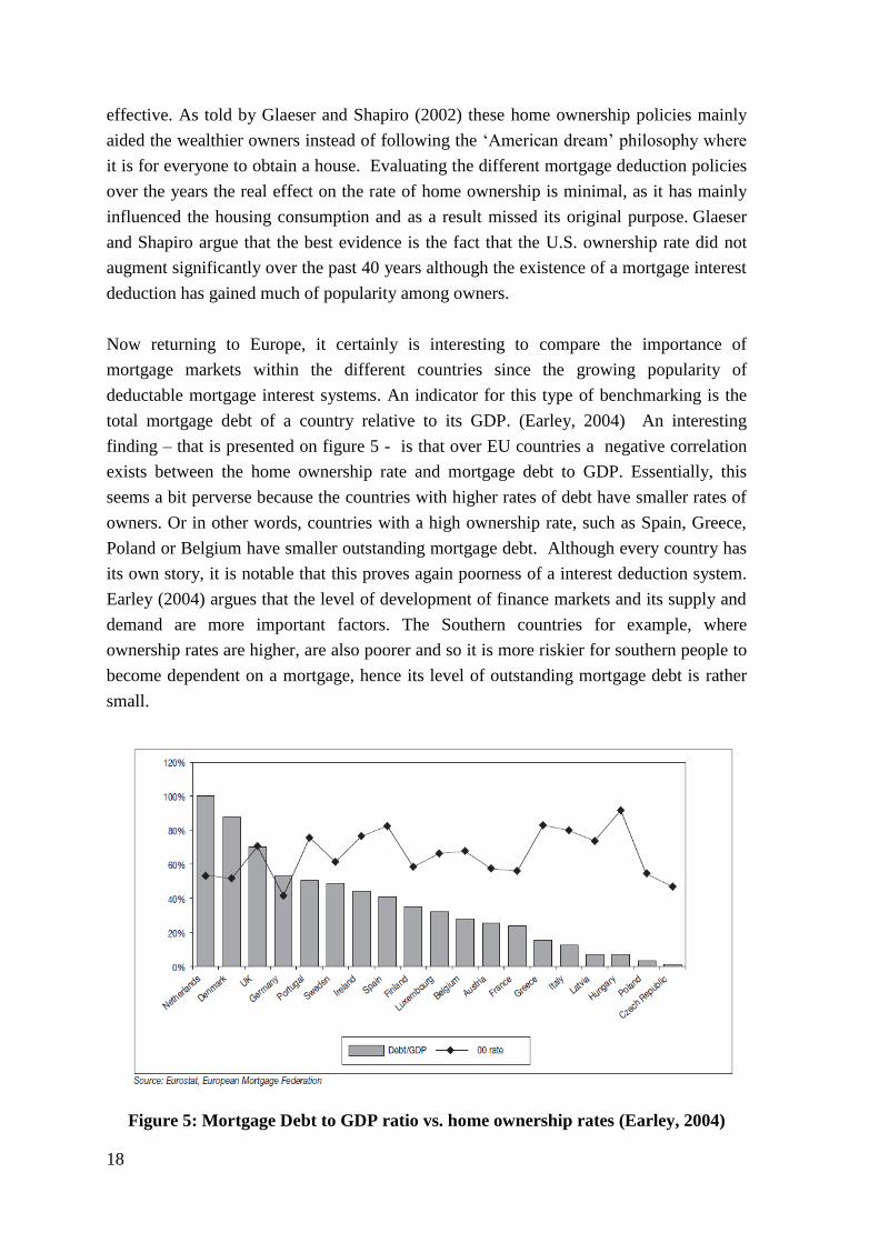
Now returning to Europe, it certainly is interesting to compare the importance of
mortgage markets within the different countries since the growing popularity of
deductable mortgage interest systems. An indicator for this type of benchmarking is the
total mortgage debt of a country relative to its GDP. (Earley, 2004) An interesting
finding – that is presented on figure 5 - is that over EU countries a negative correlation
exists between the home ownership rate and mortgage debt to GDP. Essentially, this
seems a bit perverse because the countries with higher rates of debt have smaller rates of
owners. Or in other words, countries with a high ownership rate, such as Spain, Greece,
Poland or Belgium have smaller outstanding mortgage debt. Although every country has
its own story, it is notable that this proves again poorness of a interest deduction system.
Earley (2004) argues that the level of development of finance markets and its supply and
demand are more important factors. The Southern countries for example, where
ownership rates are higher, are also poorer and so it is more riskier for southern people to
become dependent on a mortgage, hence its level of outstanding mortgage debt is rather
small.
Figure 5: Mortgage Debt to GDP ratio vs. home ownership rates (Earley, 2004)

19
2.2.4 Perverse effects of home ownership stimuli
The dream of owning your own house is widespread across Western civilization. Chasing
this dream and eventually achieving it is a self-fulfillment, a save harbor and a pleasant
thought for most people. Although ownership rates in some countries are very high,
policymakers keep pointing to the abundant benefits of owning one’s house and handle
incentives to promote this achievement. Indeed, academic literature on the benefits of
owning your own home is abundant, such as Glaeser and DiPasquale who found home
owners significantly more involved citizens which results in strong communities. On the
other hand, academics point to some perverse effects of stimulating ownership – at all
costs – for all citizens.
Credit Crisis
It’s oversimplified to find only one scapegoat for the credit crisis. In this optic the role of
home ownership is also relevant. As a result of the securitization of mortgage loans in
order to facilitate ownership to low income families, the risk that was put in the markets
was higher. Among the Americans, a perverse phenomenon rose that was named NINJA
loans that offered mortgage loans to people with No Income, No Job, or no Assets
(Coffee, 2008). At the time, prices reached higher levels relative to rent or incomes in
Ireland, Spain, the Netherlands, the United Kingdom and the United States (Diamond and
Rajan, 2009) while the general believe was that housing prices could only go up in the
long run. When the housing bubble eventually burst, the housing prices fell sharp with
corrections of 30 per cent and more (see before).
Inequality
One can also ask whether home ownership is the best way to build wealth for low-income
families. Policy makers often point to the general benefits such as the eternal rising
housing prices, that serve as a protection for the old days. Summarizing by a quote such
as “buying a house is the best investment one can make”. But is this really the full truth?
According to Galster et al. (1996) it was in 1963 that Grigsby introduced the filtering
theory of the housing market. The filtering of the housing market takes place as follows.
Prosperous citizens build new homes in new areas which are clean and modern. The
quality of these houses is outstanding, but after a few decades the quality declines
especially when these houses are not well maintained or these houses are no longer
equipped with new technologies, such as for instance energy efficient central heating.
When low-income families look for affordable houses their scope often is restricted to
these old houses that fit within their budgets. Often a miscalculation of the price is made
because future costs of maintenance are not taking into account. The fact that lower
income families tend to buy older homes that are affordable at the moment leads to higher

20
risk that the house loses its value. Especially when this old house is located in a
neighborhoods that bears a higher risk on vacancy. When demand for these houses lowers
the price will fall too. Add up a mortgage or loan that is linked to the property and this
story can even get more dangerous such as described by McCarthy, Van Zandt and Rohe
(2013). Is it fair that low income families need to make monthly mortgage repayments for
a fixed total amount that is higher as the future value of the property itself? From the
opposite point-of-view high-income families build new houses at new areas and repay a
mortgage for a total amount of which the chance that the price will rise is much higher.
Besides, the risk for low-income families is leveraged since they hold larger portions of
their wealth in housing. Therefore, Chaterjee (1996) argues that if home ownership would
not be so attractive, only households that could effort it would buy houses so there would
be smaller mortgages taken. This leads to less risk because the hold portfolios would be
more diversified.
Are HMID effective?
Mortgage deductions can even work discouraging for achieving home ownership.
Simulation models in studies have clearly shown that in some countries the value of the
deduction is capitalized into the price of the home prices themselves (Nakagami, Pareira,
1994). This certainly is a perverse effect because often young families – who often belong
to lower income groups – are financially more restrict to buy their dream. In the
simulation of Nakagami and Pareira an elimination of the interest deductibility would
mean that the price of renting becomes relatively cheaper in comparison with the price of
owning. As a result of this the rental market will bloom and as a result it will lower the
demand for houses on the housing market, which in a market economy means lowering
housing prices. What these researchers did not mention is that in real life such an
elimination may be abrupt and can lead to a shock on the housing market.
One can also question the effectiveness of offering taxation incentives for home owners.
Mann (2000) argues that countries such as Canada, New Zealand and Australia have
similar ownership rates in comparison with the U.S. despite they don’t apply HMID.
Also, when the United Kingdom reduced the deductible amounts there was no significant
drop in home ownership rates. Also for the U.S. the rate of home owners stayed rather
constant since the 1960 despite the application of HMID. (Glaeser and Shapiro, 2002)
Asset rich, income poor
Another issue an possible result of raising the home ownership rate in developed
countries is the phenomenon of “asset rich, income poor”. It describes the majority of the
elderly who have significantly higher levels of housing wealth, but are often beneath or
flirting with the poverty definition of income because pensions are less generous.

21
Research on this topic is however limited. Dolaning and Ronald (2010) point to Belgium
where this effect appears. A proposed solution for the income poorness is the reversed
mortgage in which the house is consumed in order to add an extra monthly premium to
the retirement pension income (Bradbury, 2010). In Australia Bradbury (2010)
investigated if elderly consume their housing assets during retirement. This was not really
the case. However the researcher found that the average Australian older person is indeed
asset rich but income poor.
2.3 The relation between home ownership and unemployment
This section connects the two latter sections. Next to the discussed perverse effects of
being a home owner, this section arrives at the most remarkable one among them. In
1996, British economist Andrew Oswald stated that the rising home ownership rates in
OECD countries causes higher unemployment rates (Oswald, 1996). In the pile of
academic work that followed on this statement one can distinct two levels of research that
are essential to understand the problemacy. At first level, macro academic work focuses
on the characteristics of countries or regions in order to proof the theory. Yet, a second
step of the theory has followed, that investigates the relationship on individual level. Such
a micro research is ideal to reveal the small-scale incentives of people that are underneath
the emerging correlation.
2.3.1 The Oswald Hypothesis
In 1996 Oswald published his first paper concerning the hypothesis that a rise in the
unemployment rate is explained by an increase in home ownership, or in other words a
decline of the private rental market. The original working paper shows a strong
correlation between the rate of unemployment and home ownership rate of a selection of
industrialized nations, as depicted on figure 6. Visually this positive relation is
demonstrated by a scatter plot between the two variables for a selection of industrialized
countries in the 1960s. These different countries - graphically represented by dots -
exhibit a linear relationship indicating a correlation of these two variables. Countries with
a high degree of ownership like Spain (75%) have a higher unemployment rate (18%) and
vice versa, for example, Switzerland that combines a low unemployment rate (4%) with a
low ownership rate (28%). (Oswald, 1996) However, this chart only shows a statistical
correlation. This means that unemployment and home ownership of countries tend to vary
together. However it is not known whether this relationship is causal, nor are the country
specific effects explained.
22
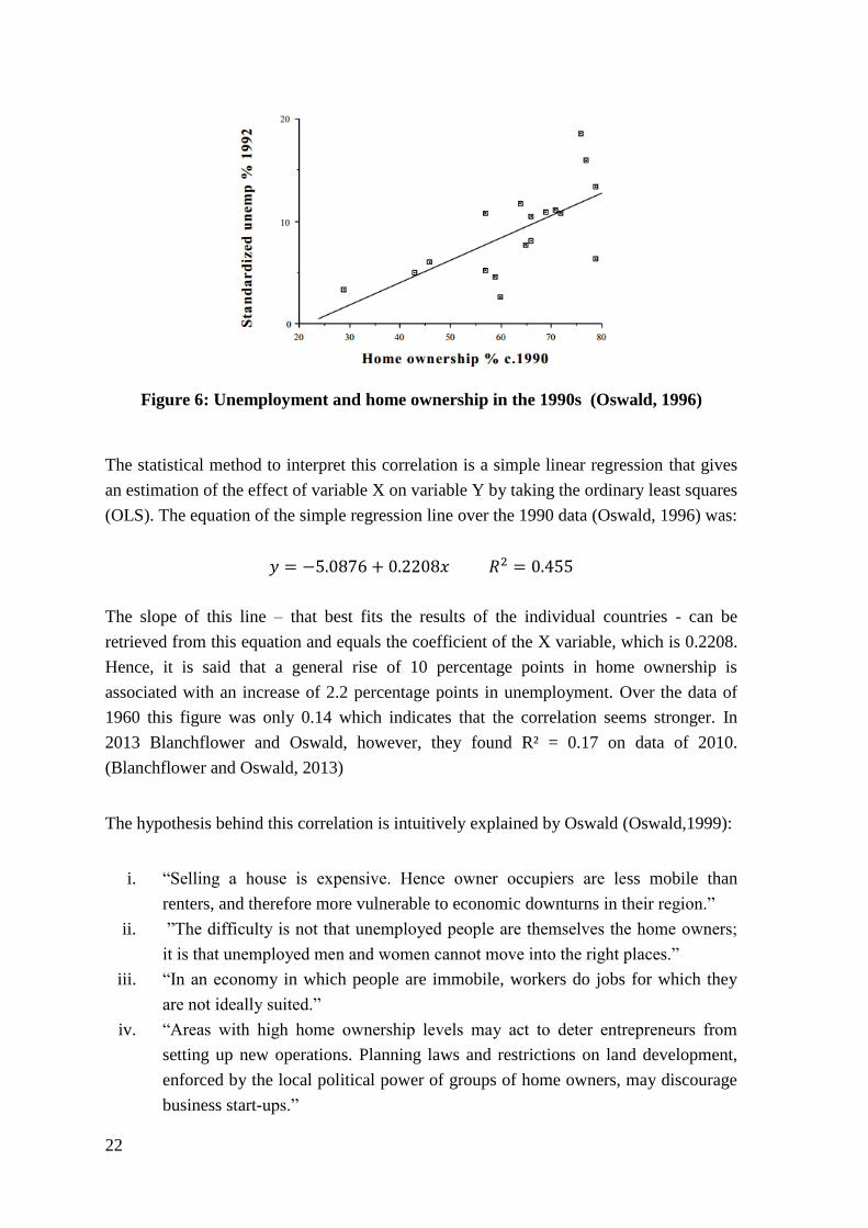
Figure 6: Unemployment and home ownership in the 1990s (Oswald, 1996)
The statistical method to interpret this correlation is a simple linear regression that gives
an estimation of the effect of variable X on variable Y by taking the ordinary least squares
(OLS). The equation of the simple regression line over the 1990 data (Oswald, 1996) was:
The slope of this line – that best fits the results of the individual countries - can be
retrieved from this equation and equals the coefficient of the X variable, which is 0.2208.
Hence, it is said that a general rise of 10 percentage points in home ownership is
associated with an increase of 2.2 percentage points in unemployment. Over the data of
1960 this figure was only 0.14 which indicates that the correlation seems stronger. In
2013 Blanchflower and Oswald, however, they found R² = 0.17 on data of 2010.
(Blanchflower and Oswald, 2013)
The hypothesis behind this correlation is intuitively explained by Oswald (Oswald,1999):
i. “Selling a house is expensive. Hence owner occupiers are less mobile than
renters, and therefore more vulnerable to economic downturns in their region.”
ii. ”The difficulty is not that unemployed people are themselves the home owners;
it is that unemployed men and women cannot move into the right places.”
iii. “In an economy in which people are immobile, workers do jobs for which they
are not ideally suited.”
iv. “Areas with high home ownership levels may act to deter entrepreneurs from
setting up new operations. Planning laws and restrictions on land development,
enforced by the local political power of groups of home owners, may discourage
business start-ups.”

23
v. “Home owners commute much more than renters, and over longer distances, and
this may lead to transport congestion that makes getting to work more costly and
difficult for everyone”
Although these arguments seem plausible they do not necessarily are true because
correlation on aggregated data is not able to prove the effects of individual persons, nor it
is possible to show a casual relation. Nonetheless, if this hypothesis is indeed correct it
would be a good explanation for the rise in the natural rate of unemployment in Europe
and other industrialized nations. So, despite this first indication, the question remains
whether unemployment is also one of these perverse effects of stimulating home
ownership across OECD countries.
2.3.2 Macro Academic Research
Early work that followed to Oswald’s working paper found evidence in favor of the
hypothesis. It was confirmed with Nickell and Layard (1999) for a selection of OECD
countries and with Green and Henderschott (2001) on U.S. data. According to Rouwendal
and Nijkamp (2007) the only exception is Spain where Barrios Garcia and Rodriguez
Hernandez (2004) found the opposite across Spanish provinces because the higher home
ownership rates were associated with lower unemployment rates. Also today the
hypothesis is often confirmed on macro data: for districts in Belgium (Isebaert et al.,
2013) and across OECD countries (Blanchflower and Oswald, 2013). These macro
studies suffer, however, from aggregation bias because the relationship between
unemployment and ownership is located on the individual level, that cannot only be
proven with aggregated data. Excessive generalizations from individuals based on these
macro data are dangerous since they can be totally opposite to reality.
Nonetheless, an interesting finding on the macro level is Germany (Lerbs, 2010) for
which Oswald’s hypothesis was investigated with data of 1998 and 2006 for the
individual Bundes Staten in Germany. A first cross-sectional estimate on these regional
data did not confirm the hypothesis. Neither a significant difference was found for the
dummy between East and West Germany. The researcher argued that factors such as
participation and productivity dominate the labor markets and thus the effect of housing
tenure is marginal. However, a fixed effects panel model found little evidence in favor of
the hypothesis that could be explained by the fact that this model is able to solve a major
problem in cross-sectional research that is called unobserved heterogeneity bias. This can
be the case if for instance a specific region has proportionally more high skilled workers
who have higher chances on being owner coincided with lower chances on being
unemployed.

24
2.3.3 Micro Academic Research
Since it is hard to make conclusions for the underlying mechanisms of the correlation at
aggregated level, academics have applied micro analysis. A scrutiny on the individual
level is advantageous because it can track and unravel the behavior mechanism(s) behind
this correlation and hence is no longer suffering from aggregation bias. So again, the
question is raised: are owners more unemployed than renters? Or do they stay longer
unemployed than renters?
A common feature that is often tested is indeed the duration of unemployment. It were
Goss and Phillips (1997) who first searched for significance with housing tenure as a
explanatory variable. Contrary to the hypothesis, ownership was found to reduce the
duration of unemployment. However, the effect for mortgagors is stronger than for
outright owners. Intuitively the incentive to work is stronger for a mortgagor because he
wants to maintain the bought house. (Nijkamp and Rouwendal, 2007)
In contrast to their macro study of 2001, Green and Hendershott (2001), did only find
little evidence on U.S. micro data from the Panel Study of Income Dynamics (PSID) with
the help of hazard equations for the effect of home ownership on the employment spell.
More specific, the relation was positive but about eight times smaller than Oswalds’
indication which is a ten per cent raise in ownership the leads to a two per cent rise in
unemployment. Also Coulson and Fisher (2002) did a micro-investigation on these PSID
data. They found no evidence at all in favor of the Oswald hypothesis because their
models showed that home owners have a smaller chance on unemployment, experience a
smaller duration of unemployment and enjoy higher wages. These contradictory results to
Oswald could be explained by the fact that some variables were not taken into account,
for example the mobility of renters or the distinction between outright owners and
mortgagors that was applied before.
Nonetheless, even today the effect seems little in the U.S. as Taskin en Yaman (2012)
used micro data over a period between 1996 and 2011. They accounted for the
unobserved heterogeneity by the use of a special model that is called the full information
maximum likelihood (FIML) method. Such a model is capable of making stable estimates
even when sets have missing values. They found that ownership does indeed reduce the
job finding hazard but again at a much smaller level than Oswald’s suggestion.
In Europe, Brunet and Lesueur (2003) went through French micro data to test if the
housing tenure is able to explain the unemployment spell. Logistic results from 3965
French individuals were however not able to reject Oswald hypothesis since home
ownership was positively related to unemployment duration. Research of Ahn and
Blazques (2007) on the European Community Household Panel (ECHP) showed mixed
25
results: Spain (no), Denmark (yes), France (weak). The researchers point remarkably to
another explanation on the effect. It seems that the degree of mobility is more a result of
satisfaction with job or home. The results of Munch et al. (2006) could clearly reject the
hypothesis for the Danish people because they found that ownership lowers the
unemployment duration. The researchers instead argue that a low labor mobility may
causes unemployment and not per se the home ownership. They argue that the effect of
ownership is not relevant for countries with low labor mobility such as in most European
countries. “By contrast in the U.S. where geographical mobility is more important on the
labor market, the effect of raising ownership may lead to higher levels of
unemployment.” (Munch et al, 2006)
In the Netherlands, research was conducted to the effects of home ownership on labor
mobility. Van Leuvensteijn en Koning (2004) could not reject the hypothesis as they
concluded: "Unemployed owners seem more likely to move than unemployed tenants."
Hence, this seems logic because Netherland has a extreme high proportion of mortgagees
that – as mentioned before by Goss and Phillips – has an impact on the financial incentive
of not wanting to lose their houses. This was also confirmed in the research of Rouwendal
and Nijkamp (2007), they found that the theory is correct Oswald for owners without a
mortgage, but not for home owners with a mortgage. This incentive was also found for
Belgium by Baert et al. (2013).
The contribution to the literature of Van Leuvensteijn and De Graaff (2007) was more
broader than the hypothesis. They found that home owners have a smaller chance on
unemployment because the researchers observed lower exit rates out of the current job
spell. They argue that it is not home ownership which has a positive effect on
unemployment, but it are the transaction costs on the housing market that causes a weaker
labor mobility.
Academic literature brings up an important problem of the results of Oswald’s hypothesis
that is named endogeneity bias. This problem is typically situated in social and economic
science and can lead to a rejection of a hypothesis that in fact is true. (Reichstein, 2013)
According to the lectures of Reichstein, the bias can be summarized underlying two
important features. First, omitted variable bias can lead to endogeneity problem such as
described by Van Leuvensteijn and Koning (2004) that certain variables in the model
have limited characteristics that are indeed important for the mechanism. The example
that the authors phrase is job commitment that can explain the housing tenure of people.
This shows that certain variables could be overlooked – or omitted - when explaining
housing tenure or the general unemployment rate model of Oswald. Second, another form
of the endogeneity problem was explained by L’Horty and Sari (2010), the simultaneity
bias. That is when variables are determined simultaneously and hence it is not clear which

26
one evokes the other one. In other words, this reverse causality can be a bias of the theory
because intuitively it is not clear whether someone is (un)employed because he is a home
owner or instead the fact that home ownership makes someone (un)employed. This latter
problem can be solved by taking lagged variables that are suffering from it. This common
practice is a good attempt, but it is not completely correct (Reed, 2013).
2.4 The role of Financial Assets and Unemployment Insurance
Literature does not only link home ownership to unemployment, as there are other
variables that can be both influential to home ownership and to unemployment. A
possible variable is the role of financial assets of which less is known in literature. For
instance, Frantantoni (1998) linked housing tenure with the relative weight of investments
in risky assets. First he showed that the average home owner has a higher amount of
financial asset than the average renter. Second, he found that a mortgage commitment is
associated to reduced risky assets holdings. Also Becker and Shabani showed that
mortgagors are 10 per cent less likely to own stocks or 37 per cent less likely to own
bonds. (Becker and Shabani, 2010) This may be a possible link in the Oswald theory.
Such a financial wealth itself may be an incentive to longer unemployment spells as it can
be consumed during the unemployed period. Gruber (2002) found that the wealth of the
unemployed population is quite diverse as it undertakes a substantial heterogeneity,
especially when measured at the start of the unemployed period. His micro data of the
1980s and 1990s were very extreme as one-third of the American workers was not even
able to replace 10 per cent of their income loss. In this paper Gruber also refers to Baily
(1978) who argued that the optimal level of unemployment insurance for a worker should
be in function of the private resources that this person can consume during the
unemployment spell. This is, in our opinion, a possible incentive for outright owners to
have longer unemployment spells because they were found to be associated with higher
financial assets, especially with higher financial risky assets.
Another relevant finding in this story is that generous unemployment insurance benefits
can undermine labor mobility. Feldstein (1973) for instance argued that indeed
unemployment insurance was responsible for a rise in unemployment rate. However, he
also found that a lot of the benefit receivers were not located especially low in the income
distribution. In this optic the Oswald theory may be specifically located with unemployed
(outright) owners that can consume both financial assets as well have an unemployment
insurance during the unemployment spell. Hence, this group has a stronger incentive for
longer unemployment spells as they can afford maintaining their living standard just as
before the unemployment period.

27
3 Data12
This paper uses the dataset of the Survey of Health, Ageing and Retirement in Europe
(SHARE) that serves data on European citizen at the age of 50 or more. In the first wave
the data extends to 30,816 observations across twelve countries while seven years later
the database of the fourth wave covers 58,489 interview individuals over fifteen European
countries plus Israel. Although the questionnaires mainly focus on lifestyle facts of the
targeted age group such as physical health or children, also information concerning
themes such as employment, housing and assets is included. Our main argument to use
this database is the fact that across most European countries unemployment is largely
situated with either young people (age -25 years) or either elder people (age 55+ years).
This latter group corresponds with the target group of SHARE survey. Furthermore, this
age group is also found to have a higher probability of being a home owner (Andrews,
Caldera Sanchez, 2011). Hence, this paper will focus on the baby boomer generation (i.e.
people born between 1946 and 1964), that at the time of the fourth wave of the SHARE
interviews in 2011, were between age 46/47 and age 64/65, which is the eldest age group
of the then labor force. In addition, we must also admit that the SHARE database is one
of these rare large-scale datasets that is freely retrievable for students.
In fact, the aim of the survey is longitudinal. In 2014 four waves were available of this
specific age group. The initial idea of making a cohort was eventually extended with a
broader database that includes more interviewees and more countries. The second wave
contains 36,730 observations of which about survived the fourth wave. Because of this
number this research was able to control for endogeneity by the use of lagged variables
out of wave 2.
Code Country (language) Wave 2 Wave 4
AT Austria 2006 and 2007 2011
DE Germany 2006 and 2007 2011 and 2012
SE Sweden 2006 and 2007 2011
NL Netherlands 2007 2011
ES Spain 2006 and 2007 2011
IT Italy 2006 and 2007 2011
FR France 2006 and 2007 2011
DK Denmark 2006 and 2007 2011
GR Greece 2007 -
12
The applied data for this paper is available in a public Dropbox folder in file name extension of (SAV).
These files can be downloaded with help of the following web link:
https://www.dropbox.com/sh/xmk4m8x09faa8le/AAAskyrODAWPVnaHnIp_U7xVa

28
C(g,i,f) Switzerland (German, Italian, French) 2006 and 2007 2011
B(f,n) Belgium (French, Dutch) 2006 and 2007 2011
CZ Czech Republic 2006 and 2007 2011
PL Poland 2006 and 2007 2011
HU Hungary 2011
PT Portugal 2011
SI Slovenia 2011
EE Estonia 2010 and 2011
(n) Number of observations 36,730 58,489
Table 2: SHARE fact sheet of wave 2 and 4 (Release Guide, 2013)
4 Methodology
This section describes the applied methodology to answer the four research questions as
mentioned in the introduction. In order to run the statistical equations on the data a
software package IBM SPSS was used, that is the abbreviation of Statistical Package for
the Social Sciences. The software’s output of the equations can be found in the appendix
C. The creation of the variables applied in following models can also be found in
appendix B. Definitions of these variables can be found in appendix A.
4.1 Oswald correlation for baby boomers across European countries (RQ1)
In 2013 Blanchflower and Oswald published a new working paper that essentially is very
similar to the original working paper by Oswald of 1996. The researchers reanalyze the
correlations with more recent figures across the OECD nations. Although the home
ownership rates have grown since the 1990, still the conclusion on the correlation is
identical, that raising ownership seems to be a good explanation of the rising
unemployment rates. On the 2010 data, the correlation coefficient of the simple
regression was found R² = 0.17. (Blanchflower and Oswald, 2013). RQ1 in this paper
applies the exact same equation (1.1) to analyze the correlations across a selection of
European countries with help of a simple regression model:
(1.1) with cn = country1, country2, …
This paper, however, only takes the baby boomer generation into account. Because of this
specific scope of age the correlation between home ownership rate (HO) and the
unemployment rate (U) is expected to be stronger for the selected countries. The selected
countries in the SHARE database for this question are Austria, Belgium, Czech Republic,
Denmark, Estonia, France, Germany, Hungary, Italy, Netherlands, Poland, Portugal,
Slovenia, Spain, Sweden and Switzerland.

29
4.2 The nuance in housing tenure (RQ2)
In the second RQ this paper scrutinizes the characteristics of the housing tenure of the
European baby boomer generation with respect of the individual countries since cultural
difference can play a important role. The applied model is a binary logit model that is
able to observe the odds ratios of the independent variables in the model on the housing
tenure. Because of the importance of the nuance in housing tenure the important
distinction is made as follows:
(a) between owners and renters, and
(b) between outright owners and mortgagor owners.
By comparing these models (model a vs. model b) this paper expects to track the
incentive of a mortgagor to be less unemployed than a outright owner, that was
mentioned in early literature of Goss and Phillips (1997) who proved the importance of
this distinction. This is in line with Rouwendal & Nijkamp (2010) and Baert et al. (2013)
who indeed pointed to the role of mortgage loans on European data. However, because of
the focus on the baby boomer generation in this paper results can be ambiguous. Because
the incentive can diverse for the elderly workers who are to reach retirement pension or in
the end of their mortgage payment scheme. In order to filter out these effects this paper
applies dummies13
for every five years in age.
The valuable characteristics that were retrieved out of the SHARE data are gender (GN),
age (AGE), household size (HHSIZE), unemployed (U) and education (EDU). Because
country fixed effects have an important role, the equation foresees 11 country dummies14
.
As a result, the statistical equations are:
(3.1.a)
with i = individual observations
4.3 The role of financial assets (RQ3)
This RQ brings a financial approach to the theory because literature has found a link
between the degree of investment decisions and the housing tenure as Frantantoni (1998)
found that higher degree of housing expenses for American renters and mortgagors led to
13
4 age categories are represented in 3 dummies (see appendix B) 14
12 countries are represented in 11 dummies (see appendix B)

30
significantly lower shares of holding risky financial assets15
. Frantantoni defined this
share of risky assets as:
In this paper an OLS regression model checks if the housing expenses (HOUSEXP) of the
mortgagors effects their choice of holding risky financial assets . It is expected that higher
mortgage repayments lead to a smaller share of risky assets . In line with Frantantoni
(1998) it is also expected that mortgagors give less weight to risky financial assets such as
stocks, bonds and mutual funds, in comparison to outright owners. Therefore, the second
model incorporates the effect of the variables housing tenure (HT) and ownership (OWN)
to the equation:
+ CN (3.4)
+ CN (3.5)
+ CN (3.6)
Whereas the housing expense ratio (HOUSEXP) is computed as:
Before these specific equations are investigated, the general role of financial assets is
scrutinized by taking the natural logarithm of financial assets as the dependant variable.
These models are presented as 3.1, 3.2, 3.2bis and 3.3.
In order to use valuable variables such as income, mortgage payments, financial assets as
a nominal variable in the regressions, it is necessary to apply an index of living standard
to correspond with the theory of the Power Purchase Parity (PPP) and the law of one price
(LOP) among the individual diverse countries. Because, intuitively, 100 Euro in Ireland
is not worth as much as 100 Euro in Slovakia. It is therefore important to eliminate these
biased effects that are regressed on the dependant variable. This paper obtains the Actual
Individual Consumption (AIC) per capita to withdraw the bias because this index takes
the price level differences between countries into account. The underneath table shows
that the diversion of the power purchase in our applied countries ranges from 63 per cent
in Hungary to 127 per cent in Switzerland over the EU28 average.
15
See appendix A for definition of financial assets

31
Country AIC per capita
Austria 1.19 Slovenia 0.81
Netherlands 1.12 Czech Republic 0.72
Sweden 1.15 Portugal 0.80
Denmark 1.13 Greece 0.92
Germany 1.23 Estonia 0.59
Belgium 1.13 Poland 0.70
France 1.14 Hungary 0.63
Italy 1.03 Switzerland 1.27
Spain 0.93 EU28 1.00
Table 3: Actual Individual Consumption (bron, jaar)
4.4 The unemployment equation (RQ4)
In this fourth RQ, the chance on unemployment is predicted with help of a logit
regression model. In Belgium Heylen (2012) refers to O’Connell et al. (2010) who
described models to predict the chance on long term unemployment (U(LT)),that are
often used by public employment services in developed countries. These original
equations take into account the following variables: gender (GN), age (AGE), marital
status (MAR), children (CH), education (EDU) and country (CN). This paper extends
such a model by adding two specific aspects that are questioned in RQ1 and RQ2. First,
the Oswald finding of housing tenure (HT) and also with the nuance of ownership status
(OWN). Second, we apply a financial approach by adding the amount of financial assets
(FA):
(4.1b and 4.2b)
Essentially, such an unemployment equation was the initial purpose of Oswald’s
methodology. However, it is not possible to make harsh conclusions on these odds ratios
since the models suffer from the endogeneity problem such as discussed in section 2.3.3.
Academic models usually address this problem with help of intstrumental variables (IV)
in a two stage least square (2SLS) regression. This paper, however, is only able to work
with lagged variables of housing tenure (HT(t-1)) and the nuanced ownership (OWN(t-1))
to address the simultaneity problem with unemployment (U). This is common practice is
in econometrics and a good attempt but not per se 100 per cent correct as argued by Reed.
(Reed, 2013). Essentially the models in RQ4 will be able to compare the effect of the
previous tenure status on the current (un)employment situation of the respondents.

32
5 Results
5.1 Descriptive summary
5.1.1 Age
As this paper concerns the baby boomer generation the most important criterion is age.
Out of the fourth wave exactly 28,374 observations belong to the baby boomer
generation, that is because they are born between 1946 and 1964. The age pyramid as
presented on figure 8 shows a structural lack of younger baby boomers that are at age 50
or younger. Therefore, dummy variables were created over every four age years so certain
categories could be excluded in case of non significance.
Figure 8: Age pyramid of the baby boomer generation in the SHARE database
(2011)
5.1.2 Unemployment rate
On average the unemployment rate for the European baby boomer generation in our
database is 9.8 per cent (N=7060). This rate was calculated in accordance with the
broader definition of being unemployed, because no specific questions concerning the
four week search period were applied in the questionnaire to build the ILO standard.
However, the average unemployment rate can be misleading because of individual
country effects. A more nuanced presentation is the following graph that shows the
individual rates for the selected countries.
6 4 2 0 2 4 6
46 yrs. 47 yrs. 48 yrs. 49 yrs. 50 yrs. 51 yrs. 52 yrs. 53 yrs. 54 yrs. 55 yrs. 56 yrs. 57 yrs. 58 yrs. 59 yrs. 60 yrs. 61 yrs. 62 yrs. 63 yrs. 64 yrs.
Males(%) Females(%) n = 28,374

33
Figure 9: Unemployment rates of the baby boomer generation (2011)
Even though the questionnaire comported a question that could make the distinction
between unemployed and looking for a job or not, only 693 observations were valid out
of the total dataset. In general 61.5 per cent of them was looking for a job, 38.5 per cent
was not.
A weak point of this paper is that it is not able to show the average unemployment spell
as this was not measured in the survey. Instead it is only possible to measure the share of
the long term unemployed out of the baby boomer work force. Unfortunately, making the
distinction between long term unemployed and short term unemployed reduces the
database significantly because only 424 observations16
out of the database have filled in
questions that can distinct long term unemployed or not. On these observations about 60.4
per cent were long term unemployed. It is however possible to distinct the countries in
Europe with flexible labor market, such as Denmark (11.1 per cent) and countries without
flexible labor markets such as Italy (71.4 per cent) and Belgium (80.2 per cent).
16
Germany, Poland and Sweden are not included in the long term unemployment section because no
observations were found.
0%
5%
10%
15%
20%
25%
30%
Unemployment Employment source: based on wave 4 of the SHARE database

34
Figure 10: Baby boomers unemployment: long term vs. short term (2011)
5.1.3 Housing tenure
The nuanced housing tenure of the baby boomer generation is very much in line with the
general Eurostat figures of the housing tenure in Europe (see paragraph 2.2, figure 4). The
baby boomer observations (N=7,060) show three countries that have a very high
percentage of tenants at a level of 40 per cent. These countries are Austria, Germany and
Switzerland. The highest percentage of ownership is Spain with 91.6 per cent and second
is Poland with 86.7 per cent. The average rate of owners over the selected countries is
77.3 per cent. Furthermore it is notable that some countries have huge percentages of
mortgagors out of the total of home owners. This benchmark is strong in line with the
debt-to-GDP ratio (see paragraph 2.2.4). For instance in Netherlands and in Switzerland
more than 90 per cent of baby boom owners still has a mortgage on the owner occupied
house. Also Denmark en Sweden have a similar high degrees of mortgagors. This is
strong in contrast to the former communist states where these percentages reach only 6
per cent for Poland and 10 per cent for Czech Republic.
0%
20%
40%
60%
80%
100%
unemployed (<2y)
LT unemployed (>2y)
source: based on wave 4 of the SHARE database
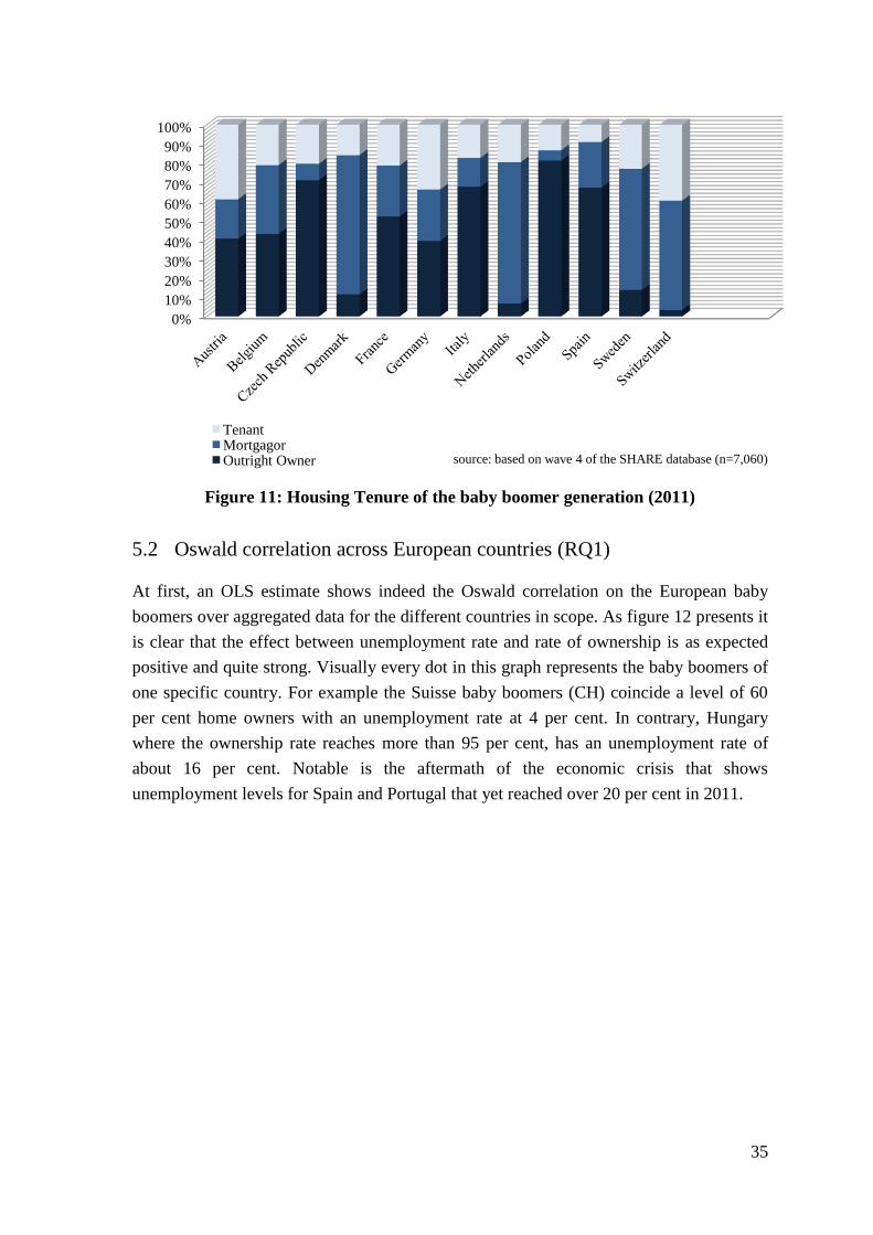
35
Figure 11: Housing Tenure of the baby boomer generation (2011)
5.2 Oswald correlation across European countries (RQ1)
At first, an OLS estimate shows indeed the Oswald correlation on the European baby
boomers over aggregated data for the different countries in scope. As figure 12 presents it
is clear that the effect between unemployment rate and rate of ownership is as expected
positive and quite strong. Visually every dot in this graph represents the baby boomers of
one specific country. For example the Suisse baby boomers (CH) coincide a level of 60
per cent home owners with an unemployment rate at 4 per cent. In contrary, Hungary
where the ownership rate reaches more than 95 per cent, has an unemployment rate of
about 16 per cent. Notable is the aftermath of the economic crisis that shows
unemployment levels for Spain and Portugal that yet reached over 20 per cent in 2011.
0%
10%
20%
30%
40%
50%
60%
70%
80%
90%
100%
Tenant Mortgagor Outright Owner source: based on wave 4 of the SHARE database (n=7,060)

36
Figure 12: General unemployment vs. home-ownership of the baby boom generation
across 16 European countries (2011)
In addition the distinction in unemployment was made between people that are
‘unemployment’ (see figure 12) and people ‘looking for a job’ (see figure 13). This first
analyses shows a strong positive correlation with slope of 0.28 that is much higher than
Blanchflower and Oswald (2013) with slope of 0.17. However, the second analysis
applied a definition of unemployment rate that is more in line with the ILO standard. The
slope of this graph (β = 0.17) is identically to Blanchflower and Oswald’s (β = 0.17). The
explanatory power of the underneath models is also very in line with their results (R² =
0.19), as figure 12 (R² 0.21) and figure 13 (R² 0.14).
Figure 13: Unemployment and home-ownership rates of the baby boom generation
across 16 European countries (2011)
A D
S
NL
ES
I F
DK CH
BE
CZ
PL
HU
P
SLO
EST
0%
5%
10%
15%
20%
25%
55% 60% 65% 70% 75% 80% 85% 90% 95% 100%
Un
emp
loym
ent
R
ate
Homeownership Rate y = 0.280x - 0.101 R² = 0.21 n = 10,158
A D
S
NL
ES
I
F
DK CH
BE
CZ
PL
HU P
SLO
EST
0%
5%
10%
15%
20%
25%
55% 60% 65% 70% 75% 80% 85% 90% 95% 100%
Un
emp
loym
ent
R
ate
(lo
oki
ng
for
a jo
b)
Homeownership Rate y = 0.178x - 0.063 R² = 0.14 n = 9,738

37
5.3 The nuance in housing tenure (RQ2)
Table 4 presents the odds ratios of the variables in the logit regression models that are
model a and model b. These odds ratios in the table need to be transformed into
probabilities in order to interpret the models:
exp (β)
The dependant variable of the first logit regression (model a) applies the distinction17
between owner (dummy = 1) and tenant (dummy = 0). According to the Oswald
hypothesis, it is expected that the probability on being owner is higher for unemployed
persons.
The odds ratios show that an unemployed person has 71.9 per cent (1-exp(0.281)) less
chance to be a home owner instead of being a tenant. Which is a first indication that the
general Oswald theory is not confirmed on these micro data. The model was expanded
with a lagged variable (model 2.3a) for unemployment18
that shows also shows a
significant negative effect of 67.9 per cent. By adding long term unemployment (model
2.4a) the effect becomes smaller to 39.4 per cent lower chance of being home owner. The
models also show that women have a smaller chance of about 22.6 per cent on being
home owner. Higher chances are found for higher educated people and for older people.
The country specific characteristics confirm the European differences again as shown in
literature and in the summary statistics. Switzerland, Austria and Germany have
significantly lower chances on having home owners in the country. Whereas, southern
and eastern European countries have a significant higher chance for example Spain and
Poland.
In the second model (b) the distinction is made between outright owner (dummy = 1) and
mortgagor (dummy = 0). Previous research has also shown that the Oswald hypothesis
was not confirmed in general, but was more precisely situated with outright owners who
are proportionally more unemployed. The explanation argues that mortgagors are less
unemployed because of the mortgage repayment incentive. The odds ratio in model 2.2b
shows that unemployed have 33.7 per cent more chance to be outright owner instead of a
mortgagor. This partially confirms the incentive of a mortgagor to be less unemployed
because of the house that needs to be paid off. However, the results for the lagged
unemployed variable and the long term unemployed are not significant. By contrast, age
increases the chance on being an outright owner quite strong. Every additive year gives
about 14 per cent more chance of being an outright owner, which is logical because
mortgages often end before retirement.
17
See also Appendix B 18
This lagged variables were constructed by implementing SHARE data of waves 2 and 4

38
Housing Tenure (model a) Ownership (model b)
# 2.1a
2.2a
2.3a
2.4a 2.1b
2.2b
2.3b
2.4b
Constant
2,171
(0,204)
2,475
(0,047)*
8,284
(0,061)
0,001
(0,000)*
0,004
(0,000)*
0,008
(0,000)*
0,098
(0,073)
0,002
(0,022)*
Gender 0,868
(0,066)
0,774
(0,000)*
0,663
(0,000)*
1,095
(0,681)
1,138
(0,201)
1,132
(0,085)
0,983
(0,893)
0,934
(0,845)
Age
1,009
(0,420)
1,014
(0,82)
1,003
(0,888)
1,140
(0,000)*
1,099
(0,000)*
1,094
(0,000)*
1,052
(0,020)*
1,137
(0,008)*
Education 1,321
(0,003)*
0,933
(0,543)
0,962
(0,914)
Householdsize 0,954
(0,639)
0,984
(0,829)
1,009
(0,950)
1,087
(0,775)
1,083
(0,547)
1,053
(0,579)
0,998
(0,992)
0,536
(0,136)
Unemployed 0,250
(0,000)*
0,281
(0,000)*
1,315
(0,170)
1,337
(0,037)*
Unemployed
(t-1)
0,321
(0,000)*
1,519
(0,145)
LT Unempl. 0,606
(0,034)*
1,261
(0,510)
Austria 0,459
(0,000)*
0,395
(0,000)*
0,331
(0,009)*
0,734
(0,318)
2,656
(0,000)*
1,764
(0,000)*
0,658
(0,331)
Germany 0,487
(0,000)*
0,320
(0,000)*
1,594
(0,421)
0,902
(0,574)
0,743
(0,205)
Sweden 0,694
(0,754)
0,706
(0,042)*
0,400
(0,000)*
0,000
(0,999)
0,124
(0,000)*
0,111
(0,000)*
Netherlands 0,966
(0,793)
0,575
(0,032)*
1,594
(0,421)
0,064
(0,000)*
0,062
(0,000)*
Spain 4,522
(0,000)*
3,191
(0,000)*
1,346
(0,388)
5,736
(0,000)*
3,193
(0,000)*
2,213
(0,000)*
1,819
(0,026)*
Italy 1,471
(0,048)*
1,124
(0,438)
0,804
(0,484)
2,602
(0,120)
5,902
(0,000)*
3,845
(0,000)*
2,494
(0,001)*
France 1,292
(0,215)
0,925
(0,559)
0,472
(0,002)*
0,908
(0,865)
2,195
(0,000)*
1,658
(0,000)*
1,324
(0,200)
Denmark 1,334
(0,172)
1,209
(0,170)
0,756
(0,261)
11,757
(0,025)*
0,174
(0,000)*
0,120
(0,000)*
0,096
(0,000)*
Switzerland 0,395
(0,000)*
0,336
(0,000)*
0,168
(0,000)*
0,288
(0,016)*
0,058
(0,000)*
0,045
(0,000)*
0,056
(0,000)*
Czech
Republic
1,117
(0,440)
0,982
(0,874)
0,920
(0,795)
1,712
(0,120)
10,450
(0,000)*
7,246
(0,000)*
6,259
(0,000)*
Poland 1,913
(0,012)*
1,314
(0,061)
0,001
(0,000)*
11,186
(0,000)*
7,872
(0,000)*
Nagelkerke R² ,131 ,116 0.112 0.240 0.489 0.480 0.480
0.085
N 3805 7018 2240 421 2699 5209 1742 179
Table 4: Odds ratios (Exp(β)) of housing tenure in RQ 2

39
5.4 The role of financial assets (RQ3)
The underneath table presents the quartiles in financial assets across the different housing
categories. These financial assets are converted in euro and converted into the same
purchase power by implementing the AIC (see section 4.3). It is remarkable that financial
assets of mortgagors are significantly higher than outright owners. This can partially be
explained by the fact that northern countries are richer and have proportionally more
mortgage owners, while southern and eastern countries are poorer and have
proportionally more outright owners.
Mortgagor Outright owner Tenant
25 € 3751.82 € 319.56 € 349.17
50 € 25000.00 € 3465.13 € 3100.00
75 € 89804.75 € 21180.83 € 20128.28
n 3396 9592 3768
Table 5: Financial assets in quartiles per housing tenure
The results in table 6 below indeed confirm that mortgagors are related to higher amounts
of financial assets (model 3.2). However, once country specific effects are added by
dummies (model 3.2bis), the coefficients show remarkable significant differences among
the European countries. For example Suisse people have significant higher financial
assets than the reference group. Unfortunately, the nuanced ownership status does no
longer make a substantial difference in this model (3.2bis). Yet R² augments from 9.3 to
24.3 per cent. This confirms that the differences in financial assets are mainly explained
by the country specific effects. Furthermore, higher amounts of financial assets in the
financial portfolio are also associated with males, higher educated and married people.
Looking deeper into this mortgagor group it is clear that higher housing expense ratio is
negatively related with the amount of financial assets (model 3.3). In other words, high
commitment mortgagors have lower amounts of financial assets. Besides, higher housing
expense ratios are also associated with higher weights of risky assets (model 3.6). This is
the opposite to the conclusion of Frantantoni (1998) but can be caused by too few
observations (N = 132).
The last remarkable finding is that owners, in comparison with tenants, are associated
with significant smaller weights of risky financial assets. Specifically, this weight seems
to be higher in Spain and lower in countries such as France and Czech Republic.

40
Ln_PPP_Financial Assets Relative weight of Risky Assets
# 3.1 3.2 3.2bis 3.3 3.4 3.5 3.6
Constant
Housing Tenure 0.139
(0.000)*
-0.101
(0.003)*
Outright Owner
-0.198
(0.000)*
0.024
(0.246)
0.007
(0.839)
Housing Expense Ratio -0.102
(0.029)*
0.235
(0.009)*
Age 0.025
(0.072)
0.015
(0.273)
0.003
(0.873)
0.056
(0.209)
0.155
(0.000)*
0.151
(0.000)*
0.046
(0.602)
Gender -0.087
(0.000)*
-0.149
(0.000)*
-0.105
(0.000)*
-0.059
(0.208)
0.032
(0.337)
-0.011
(0.749)
-0.050
(0.570)
Education 0.148
(0.000)*
0.074
(0.000)*
0.152
(0.000)*
0.275
(0.000)*
0.012
(0.751)
-0.030
(0.376)
0.121
(0.171)
Married 0.094
(0.000)*
0.095
(0.000)*
0.062
(0.000)*
0.119
(0.008)*
0.011
(0.736)
0.009
(0.786)
0.089
(0.355)
Germany 0.020
(0.128)
0.025
(0.093)
0.020
(0.540)
Sweden 0.022
(0.089)
0.040
(0.008)*
0.012
(0.709)
Spain -0.035
(0.020)*
-0.008
(0.647)
0.100
(0.003)*
Italy 0.026
(0.075)
0.004
(0.010)*
0.196
(0.000)*
France 0.161
(0.000)*
0.213
(0.000)*
-0.130
(0.001)*
Denmark 0.106
(0.000)*
0.146
(0.000)*
-0.004
(0.908)
Switzerland 0.355
(0.000)*
0.398
(0.000)*
Czech Republic -0.015
(0.327)
-0.009
(0.613)
-0.114
(0.001)*
Poland 0.005
(0.704)
0.005
(0.739)
Adjusted R² 0.230 0.093 0.243 0.118 0.122 0.020 0.029
N 4428 5910 3342 456 874 948 132
Table 6: Risky financial assets and financial assets (RQ3)

41
5.5 The unemployment equation (RQ4)
The chance on unemployment is predicted with help of logit regression models. Table 7
presents the results of two series of models. The first models have unemployment as the
dependant variable, while the second models have long term unemployment as the
dependant variable. Long term unemployment is defined as people who are unemployed
for more than two years. The models below are free of multicollinearity and outliers that
were taken into account because of a possible correlation between education, financial
assets and the tenure states. Because the country specific results in model 4.3a are
confusing as a result of the 2011 skyrocketing unemployment rates in Spain and Portugal
the dummy variables were withhold in the other models because skewed observations
lead to indecisive results.
Similar as in RQ1 the results below confirm that home owners have smaller chance on
unemployment in comparison with renters. In this dataset this chance is about 42 per cent
smaller for home owners, which is very similar to the micro data model of Coulson and
Fisher (2002) that found approximately 35 per cent19
less chance in the United States.
Remarkable is when a five year lagged variable of housing tenure is added to the model
(4.2a), it does not show a significant stronger effect on the current unemployment
situation of the observed persons. Although, it seems that the Oswald hypotheses is
rejected again on micro level, the nuance in ownership shows a significant higher chance
for outright owners to be unemployment in comparison with mortgagors. This is very
much in line with literature such as Nijkamp and Rouwendal (2007) and points to the
incentive of mortgagors to be employed in order to make mortgage repayments for the
acquired house. This time the lagged variable makes the relation significantly stronger,
which is a remarkable confirmation of the latter finding.
The role of financial assets shows an obvious relation towards unemployment. A one
percent raise in financial assets leads to a significant smaller chance on unemployment. In
other words people with small financial assets are proportionally more unemployed.
The results of the long term unemployment equations are similar although they reveal that
women and elder people have significantly higher chances of being long term
unemployed. Which is in line with the findings of Rones (1983) that described longer
unemployment spells for older workers and for women.
19
Coulson and Fisher (2002), p 44: probability = 1 – exp(-0.43515)

42
Unemployment Long Term
Unemployent
# 4.1a
4.2a 4.3a
4.4a
4.5a 4.1b
4.2b
Constant
0,049
(0,079)
0,022
(0,020)*
0,242
(0,447)
0,003
(0,015)*
0,038
(0,112)
0,002
(0,074)
0,004
(0,038)*
Housing Tenure 0,572
(0,018)*
0,506
(0,008)*
0,514
(0,183)
Housing Tenure(t-1) 0,545
(0,000)*
Outright Owner
2,129
(0,029)*
1,159
(0,7005)
Outright Owner(t-1) 2,367
(0,000)*
PPP Financial Assets
(log)
0,713
(0,000)*
0,727
(0,000)*
0,625
(0,000)*
0,617
(0,001)*
Gender 0,746
(0,190)
0,881
(0,420)
0,771
(0,263)
0,805
(0,474)
1,046
(0,815)
1,067
(0,888)
2,069
(0,039)*
Education 0,294
(0,000)*
0,410
(0,001)*
0,272
(0,000)*
0,675
(0,393)
0,565
(0,113)
Age 1,096
(0,000)*
1,036
(0,202)
1,072
(0,023)*
1,145
(0,001)*
1,007
(0,840)
1,209
(0,003)
1,100
(0,042)*
Low Urbanization 0,797
(0,368)
0,868
(0,591)
1,264
(0,611)
Medium Urbanization 1,136
(0,693)
1,358 1,176
(0,770)
Country of birth 1,898
(0,027)*
1,624
(0,108)
1,257
(0,677)
0,430
(0,168)
0,835
(0,760)
Married 0,653
(0,066)
0,693
(0,133)
0,880
(0,705)
2,185
(0,085)
1,249
(0,571)
Austria 0,503
(0,047)*
Spain 1,220
(0,605)*
Italy 0,241
(0,019)*
France 0,339
(0,072)
Denmark 0,156
(0,019)*
Switzerland 0,307
(0,005)*
Czech Republic 0,228
(0,001)*
Nagelkerke R² 0,222 0,017 0,268 0,262 0,032 0,286 0,107
N 1297 1873 1297 992 1437 115 157
Table 7: Odds ratios in the unemployment equation (RQ4)
43
6 Conclusion
This papers investigated the Oswald hypothesis at micro level on a dataset of the
European baby boomer generation and implements two important features. First the
characteristics of the nuanced ownership status were scrutinized (see RQ2). Second, a
financial approach was brought to the theory in order to check whether the tenure choice
is associated with higher (or lower) amounts of financial assets (see RQ3). Finally, these
findings are brought together in an unemployment equation to investigate whether this
features have a significant impact on the boomers’ chance of being unemployed (see
RQ4).
The first cross sectional analysis (see RQ1) concerned the relationship between
unemployment rate and home ownership rate on aggregated country level. These results
clearly show - in line with most macro analyses - that a strong positive relationship exists
between these indicators. However, it does not explain the underlying mechanism.
Therefore, the relation is investigated at micro level with the previous mentioned RQ’s.
This was done with help of SPSS on the database of the SHARE survey.
At this micro level the results (see RQ2) show that unemployed people have a smaller
chance of being a home owner instead of a renter, which means that the Oswald
hypothesis is rejected. However, looking more deeply in this relationship, the nuance of
ownership shows that mortgagors have 30 per cent less chance on unemployment, and
hence unemployment is strongly related with outright owners. This confirms the
expectation of the incentive of mortgagors to be employed in order to pay off their
mortgage loans as they do not want to lose their acquired house.
The financial approach (RQ3) shows that owners, overall, own more financial assets than
tenants. More specifically, it are mortgagors who own significantly the most financial
assets than outright owners and tenants. The explanation for this may be country specific
because northern countries that are richer have proportionally more mortgagors, while
southern and eastern countries are poorer and have proportionally more outright owners.
For this mortgagor group it is also found that high mortgage repayment-to-income ratios
are associated with low amounts of financial assets. Or in other words, mortgagors who
own high financial assets do not take as much risk as people with low financial assets in
order to pay off their house.
Contrary to Frantantoni (1998) we find that in Europe the risk in the financial portfolio is
positively associated with risk in mortgage repayments. This seems not logic, but this
ambiguity may be the result of the country-specific expects within Europe that could not
be included in this last analysis. However, this points again to the major importance of

44
these country specific results for European research.
Taking everything together in the unemployment equation (RQ4) it is found that people
with small financial assets are proportionally more unemployed. Also it was found that
home ownership and more specific mortgagees have a smaller chance of being
unemployed, confirming the results of RQ2 and the many micro literature such as
suggested by Henley (1998), and confirmed by Nijkamp and Rouwendal (2007) and also
found by Baert et al. (2013).
7 Final remarks of the authors
Our statistics show that most European baby boomers succeeded very well in owning
their own homes before the age of 65. However, this is not per se a good thing for our
economy as we show that outright owners are associated with higher chances on
unemployment and lower amounts of financial assets. This seems to be an indication that
the phenomenon of “asset rich and income poor” may be one of the most important
challenges for policy makers in the upcoming decades. Especially because the European
baby boomer generation is abundant and is getting in retirement since 2011. Despite,
European policies in the last three decades have been focusing on pension reforms of the
legal state pensions (Holzmann, 2003) economist are not yet convinced if our economies
can keep contributing to the status quo of old age pensions. Some of them even compare
the social security pension systems with a Ponzi scheme. (Tanner, 2011)
Also, we saw a rising consensus in the academic world that fiscal ownership stimuli have
perverse effects for lower income groups that are not socially acceptable. Therefore the
academic consensus argues that policy makers should be tenure neutral instead of
stimulating ownership.
Concerning future research on the Oswald theory we advise to incorporate the financial
wealth as this may play an important role in the incentive to work or not. Especially in
Europe, where unemployment insurance is more generous. We were however not able to
scrutinize the incentive of unemployed outright owners to stay longer unemployed when
they own significant amounts of financial assets. This remains a question.
Moreover, further research on the specific baby boomer generation can be conducted in
the near future because a fifth wave of the SHARE survey will be released in 2015.
Hence this research will be able to make longitudinal analyses at micro level.

45
8 References
Ahn, M., & Blázquez, M. (2007). Residential mobility and labor market transitions: relative effects of
housing tenure, satisfaction and other variables. Documento de trabajo, 07-05.
Andersen, T. M., & Svarer, M. (2007). Flexicurity—labour market performance in Denmark. CESifo
Economic Studies, 53(3), 389-429.
Andrews, D., Sánchez, A. C., & Johansson, Å. (2011). Housing markets and structural policies in OECD
countries. OECD.
Baert, Stijn, Heylen, F., & Isebaert, D. (2013). Does homeownership lead to longer unemployment spells?
The role of mortgage payments. Working Paper Series - Faculty of Economics and Business
Administration, Ghent University.
Baily, M. N. (1978). Some aspects of optimal unemployment insurance.Journal of Public
Economics, 10(3), 379-402.
Battu, H., Ma, A., & Phimister, E. (2008). Housing Tenure, Job Mobility and Unemployment in the
UK*. The Economic Journal, 118(527), 311-328.
Becker, T. A., & Shabani, R. (2010). Outstanding debt and the household portfolio. Review of Financial
Studies, 23(7), 2900-2934.
Blanchard, O. (2006). European unemployment: the evolution of facts and ideas. Economic policy, 21(45),
5-59.
Blanchard, O., & Katz, L. F. (1996). What we know and do not know about the natural rate of
unemployment (No. w5822). National Bureau of Economic Research.
Blanchflower, D. G., & Oswald, A. J. (2013). Does high home-ownership impair the labor market? (No.
w19079). National Bureau of Economic Research.
Bourassa, S. C., Haurin, D. R., Hendershott, P. H., & Hoesli, M. (2013). Determinants of the Home
ownership Rate: An International Perspective.Swiss Finance Institute Research Paper, (11-49).
Bover, O., Casado, J. M., Costa, S., Du Caju, P., McCarthy, Y., Sierminska, E., ... & Zavadil, T.
(2013). The distribution of debt across euro area countries: The role of individual characteristics,
institutions and credit conditions (No. 252).
Bradbury, B. (2010). Asset rich, but income poor: Australian housing wealth and retirement in an
international context. Department of Families, Housing, Community Services and Indigenous Affairs.
Brandolini, A., Cipollone, P., & Viviano, E. (2006). Does the ILO definition capture all
unemployment?. Journal of the European Economic Association,4(1), 153-179.
Bratt, R. G. (2002). Housing for very low-income households: the record of President Clinton, 1993-
2000 (No. 8). Joint Center for Housing Studies, Harvard University.
Brunet, C., & Lesueur, J. Y. (2003). Do home owners stay unemployed longer? A French micro-
econometric study.
Bush, G. W. (2003). President calls on Senate to pass American Dream Downpayment Act. 2003a
[Internet]. Dinuba, CA: The White House, 20031015-10, consulted on February 20, 2014
46
Carliner, M. S. (1998). Development of federal home ownership “policy”.Housing Policy Debate, 9(2),
299-321.
Case, K. E., & Shiller, R. J. (1989). The behavior of home buyers in boom and post-boom markets. New
England Economic Review, pp. 29-46,
Case, K. E., & Shiller, R. J. (2003). Is there a bubble in the housing market?.Brookings Papers on
Economic Activity, 2003(2), 299-362.
Charlton, J., Kelly, S., Dunnell, K., Evans, B., Jenkins, R., & Wallis, R. (1992). Trends in suicide deaths in
England and Wales. Population trends, (69), 10-6.
Chatterjee, S. (1996). Taxes, Home Ownership, and the Allocation of Residential Real Estate
Risks. Business Review, (Sep), 3-10.
Clinton, W.J., (1995, June), Remarks on the National Home ownership Strategy, Online by Gerhard Peters
and John T. Woolley, The American Presidency Project. http://www.presidency.ucsb.edu/ws/?pid=51448.
Coffee Jr, J. C. (2008). What Went Wrong-A Tragedy in Three Acts. U. St. Thomas LJ, 6, 403., consulted
on 12 February 2014
Coulson, N. E., & Fisher, L. M. (2002). Tenure choice and labour market outcomes. Housing
Studies, 17(1), 35-49.
de Graaff, T., & van Leuvensteijn, M. (2007). The impact of housing market institutions on labour
mobility. CPB Netherlands Bureau for Economic Policy Analysis, Discussion Paper, (82).
Diamond, D. W., & Rajan, R. (2009). The credit crisis: Conjectures about causes and remedies (No.
w14739). National Bureau of Economic Research.
DiPasquale, D., & Glaeser, E. L. (1999). Incentives and social capital: are home owners better
citizens?. Journal of urban Economics, 45(2), 354-384.
Doling, J., & Ronald, R. (2010). Home ownership and asset-based welfare.Journal of housing and the built
environment, 25(2), 165-173.
Doms, M., & Motika, M. (2006). The rise in home ownership. FRBSF Economic Letter, 30.
Drehmann, M., Borio, C. E., & Tsatsaronis, K. (2012). Characterising the financial cycle: don't lose sight of
the medium term!.
Earley, F. (2004). What explains the differences in home ownership rates in Europe. Housing Finance
International, 19, 25-30.
Feldstein, M. S. (1973). Lowering the Permanent Rate of Unemployment. U.S. Government Printing
Office, Washington, D.C. 20402
Feldstein, M. S. (1997). The costs and benefits of going from low inflation to price stability. In Reducing
inflation: Motivation and strategy (pp. 123-166). University of Chicago Press.
Fisher, L. M., & Jaffe, A. J. (2003). Determinants of international home ownership rates. Housing finance
international, 18(1), 34-37.
Flatau, P., Forbes, M., & Hendershott, P. H. (2003). Home ownership and unemployment: the roles of
leverage and public housing (No. w10021). National Bureau of Economic Research.
Fratantoni, M. C. (1998). Home ownership and investment in risky assets.Journal of Urban
Economics, 44(1), 27-42.

47
Friedman, M.. "The role of monetary policy." The American Economic Review 58.1 (1968).
Galster, G. (1996). William Grigsby and the analysis of housing sub-markets and filtering. Urban
Studies, 33(10), 1797-1805.
Glaeser, E. L., & Shapiro, J. M. (2002). The benefits of the home mortgage interest deduction (No. w9284).
National Bureau of Economic Research.
Goss, E. P., & Phillips, J. M. (1997). The impact of home ownership on the duration of unemployment. The
Review of Regional Studies, 27(1), 9-27.
Green, R. K., & Hendershott, P. H. (2001). Home-ownership and the duration of unemployment: a test of
the Oswald hypothesis. NBER Working paper.
Green, R. K., & Hendershott, P. H. (2001). Home-ownership and unemployment in the US. Urban
Studies, 38(9), 1509-1520.
Gruber, J. (2001). Wealth of the Unemployed, The. Indus. & Lab. Rel. Rev.,55, 79.
Holzmann, R., & Palmer, E. (2006). Pension reform. Washington, DC.
International Conference of Labour Statisticians (1982, October), International Labour Organization (ILO)
Resolutions Concerning Economically Active Population, Employment, Unemployment and
Underemployment Adopted by the 13th, October 1982, para. )
Isebaert, D., Heylen, F., & Smolders, C. (2013). Houses and/or jobs: ownership and the labour market in
Belgian districts. Regional Studies, (ahead-of-print), 1-20.
Kirchgässner, G., & Pommerehne, W. W. (1996). Tax harmonization and tax competition in the European
Union: Lessons from Switzerland. Journal of Public Economics, 60(3), 351-371.
Krugman, P. (1983, October). International Aspects of US Monetary and Fiscal Policy. In paper for the
Bald Peak Conference sponsored by the Federal Reserve Bank of Boston.
L’Horty, Y., & Sari, F. (2010). Home-ownership and unemployment: A test of the Oswald hypothesis for the
Paris region. Working Paper.
Lerbs, O. (2010). Does home ownership really cause unemployment? Evidence from German regional
data. Preliminary draft, 22p.
Lucas Jr, R. E. (1976, December). Econometric policy evaluation: A critique. In Carnegie-Rochester
conference series on public policy (Vol. 1, pp. 19-46). North-Holland.
Malkiel, B. G., & Fama, E. F. (1970). Efficient capital markets: A review of theory and empirical
work*. The journal of Finance, 25(2), 383-417.
Mann, R. F. (2000). (Not So) Little House on the Prairie: The Hidden Costs of the Home Mortgage Interest
Deduction, The. Ariz. St. LJ, 32, 1347.
Meltzer, A. H. (2010). A History of the Federal Reserve, Volume 2. University of Chicago Press.
Munch, J. R., Rosholm, M., & Svarer, M. (2006). Are Home owners Really More Unemployed?*. The
Economic Journal, 116(514), 991-1013.
Nakagami, Y., & Pereira, A. M. (1991). Housing appreciation, mortgage interest rates, and home owner
mobility. Journal of Urban Economics, 30(3), 271-292.

48
Neider, C. (1959). The Autobiography of Mark Twain.
Nickell, S., & Layard, R. (1999). Labor market institutions and economic performance. Handbook of labor
economics, 3, 3029-3084.
Oswald, A. (1999). The housing market and Europe’s unemployment: a non-technical paper. Home
ownership and the labour Market in Europe, 43-52.
Oswald, A. J. (1997). HAPPINESS AND ECONOMIC PERFORMANCE*. The Economic
Journal, 107(445), 1815-1831.
Platt, S., & Kreitman, N. (1990). Long term trends in parasuicide and unemployment in Edinburgh, 1968–
87. Social psychiatry and psychiatric epidemiology, 25(1), 56-61.
Proxenos, S. (2002). Home ownership rates: a global perspective. Housing finance international, 17(2), 3-7.
PWC (2012), Spain restricts the tax deductibility of interest expence, M&A Tax Newsalert, retrieved from
the website on February, 12, 2014
Reagan, R. (1966, April), Speech of the Governor of California, speech presented in Sacramento Bee,
California, U.S.
Reed, W. R. (2013). ON THE PRACTICE OF LAGGING VARIABLES TO AVOID SIMULTANEITY.
Department of Economics and Finance, University of Canterburty, Christchurch, New Zealand
Reichstein, T. (2013), Econometrics: Endogeneity and Instrumental Variables Regressions, Department of
Innovation and Organizational Economics, Copenhagen Business School, powerpoint presentation at online
website at http://www.soc.aau.dk/fileadmin/user_upload/kbm/VoF/Kurser/2011/kvantitative-
metoder/Slides/TR-Endogeneity.pdf, consulted on February 19, 2014
Rix, S. E. (2013). 2. Public policy for an ageing workforce: how does the US compare?. Older Workers in
an Ageing Society: Critical Topics in Research and Policy, 19.
Rohe, W. M., & Stegman, M. A. (1994). The impact of home ownership on the social and political
involvement of low-income people. Urban Affairs Review, 30(1), 152-172.
Rohe, W. M., Van Zandt, S., & McCarthy, G. (2013). The social benefits and costs of home ownership: A
critical assessment of the research. Affordable Housing Reader MUELLER & TIGHE, 196.
Roll, R. (2003). Benefits to home owners from mortgage portfolios retained by Fannie Mae and Freddie
Mac. Journal of Financial Services Research,23(1), 29-42.
Rones, P. L. (1983). Labor Market Problems of Older Workers, The. Monthly Lab. Rev., 106, 3.
Rouwendal, J., & Nijkamp, P. (2007). Home ownership and labour market behaviour: interpreting the
evidence (No. 07-047/3). Tinbergen Institute Discussion Paper.
Shiller, R. J. (2000). The Irrational Exuberance.
Shiller, R. J. (2013, December). Exclusive interview with Nobel laureate in economics, interview on SVT
channel Sweden. Consulted on March, 25, 2014
Solow, R. M. (2000). Unemployment in the United States and in Europe: A Contrast and the Reasons.
CESifo.

49
Struyk, R. J. (2000). Home ownership and Housing Finance Policy in the Former Soviet Bloc-Costly
Populism.
Taskın, A. A., & Yaman, F. (2012). Home ownership and Unemployment Duration: Different
Opportunities, Different Outcomes.
Tanner, M. (2011). Social Security, Ponzi Schemese, and the Need for Reform. Cato Institute Policy
Analysis, (689).
Tatsiramos, K. (2006). Residential mobility and housing adjustment of older households in Europe (No.
2435). IZA Discussion Papers.
U.S. Department of Commerce (1942), Eight annual report of the federal housing administrationg,
published by the U.S. Government Printing Office in Whasington
Van Leuvensteijn, M., & Koning, P. (2004). The effect of home-ownership on labor mobility in the
Netherlands. Journal of Urban Economics, 55(3), 580-596.

50
Appendix A
Home owner
Our definition of home ownership is in line with academic literature. The owner or co-
owner lives in an housing unit that he or she occupies with his or her household. A
mortgage linked to this housing unit does not change the status of the owner-occupier.
Tenant
Oxford Dictionary states: “a tenant is a person who occupies land or property rented from
a landlord.”. This paper defines the status of ‘under tenant’ also as a tenant. However,
free residents and members of cooperations were excluded from our definition of tenants.
Mortgagor
This is a owner-occupier who has an outstanding loan or mortgage linked to the property
of which he is the owner-occupier.
Outright Owner
This is a owner-occupier who has no outstanding loan or mortgage linked to the property
that he owns and occupies.
Home ownership Rate
This rate equals the total number of home owners divided by the sum of home owners and
tenants.
Unemployment
Only Wave 4 makes the discrepancy between the real situation of being unemployed and
looking for a job. Which is more or less in line with the definition of the International
Labour Organisation (ILO).
Long Term Unemployment
The respondent is perceived as long term unemployed in case this person reported to be
unemployed for more than two years.
Unemployment Rate
Both Eurostat and the OECD defines the unemployment rate as the fraction of total
unemployed persons in relation to the total labor force. This latter is the sum of the
employed people plus the unemployed people. (This definition is based on the
International Labour Organisation – ILO.). Wave 1 and Wave 2 do not distinct the
fraction of unemployed people that have the actual intention to look for a job.
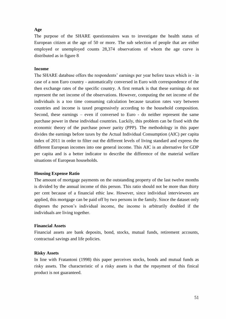
51
Age
The purpose of the SHARE questionnaires was to investigate the health status of
European citizen at the age of 50 or more. The sub selection of people that are either
employed or unemployed counts 28,374 observations of whom the age curve is
distributed as in figure 8.
Income
The SHARE database offers the respondents’ earnings per year before taxes which is - in
case of a non Euro country - automatically conversed in Euro with correspondence of the
then exchange rates of the specific country. A first remark is that these earnings do not
represent the net income of the observations. However, computing the net income of the
individuals is a too time consuming calculation because taxation rates vary between
countries and income is taxed progressively according to the household composition.
Second, these earnings – even if conversed to Euro - do neither represent the same
purchase power in these individual countries. Luckily, this problem can be fixed with the
economic theory of the purchase power parity (PPP). The methodology in this paper
divides the earnings before taxes by the Actual Individual Consumption (AIC) per capita
index of 2011 in order to filter out the different levels of living standard and express the
different European incomes into one general income. This AIC is an alternative for GDP
per capita and is a better indicator to describe the difference of the material welfare
situations of European households.
Housing Expense Ratio
The amount of mortgage payments on the outstanding property of the last twelve months
is divided by the annual income of this person. This ratio should not be more than thirty
per cent because of a financial ethic law. However, since individual interviewees are
applied, this mortgage can be paid off by two persons in the family. Since the dataset only
disposes the person’s individual income, the income is arbitrarily doubled if the
individuals are living together.
Financial Assets
Financial assets are bank deposits, bond, stocks, mutual funds, retirement accounts,
contractual savings and life policies.
Risky Assets
In line with Fratantoni (1998) this paper perceives stocks, bonds and mutual funds as
risky assets. The characteristic of a risky assets is that the repayment of this finical
product is not guaranteed.
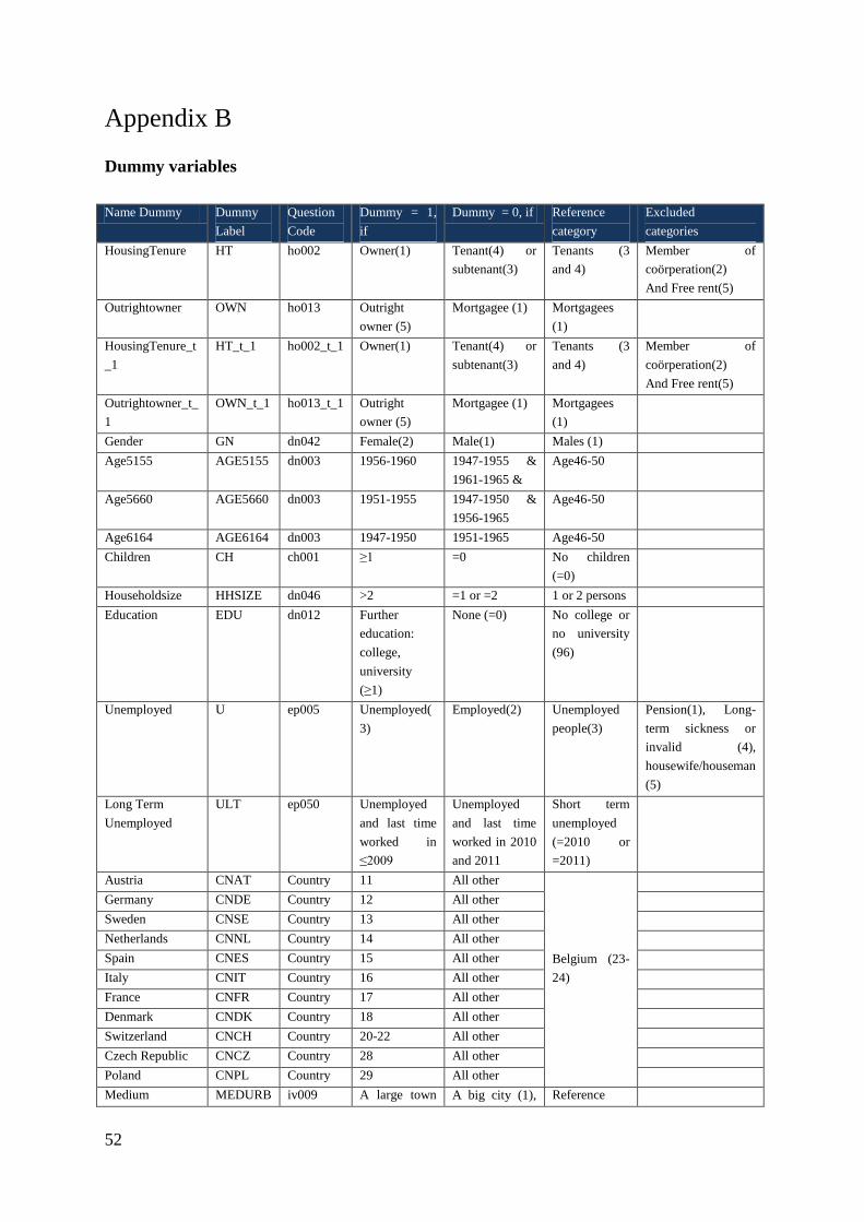
52
Appendix B
Dummy variables
Name Dummy Dummy
Label
Question
Code
Dummy = 1,
if
Dummy = 0, if Reference
category
Excluded
categories
HousingTenure HT ho002 Owner(1) Tenant(4) or
subtenant(3)
Tenants (3
and 4)
Member of
coörperation(2)
And Free rent(5)
Outrightowner OWN ho013 Outright
owner (5)
Mortgagee (1) Mortgagees
(1)
HousingTenure_t
_1
HT_t_1 ho002_t_1 Owner(1) Tenant(4) or
subtenant(3)
Tenants (3
and 4)
Member of
coörperation(2)
And Free rent(5)
Outrightowner_t_
1
OWN_t_1 ho013_t_1 Outright
owner (5)
Mortgagee (1) Mortgagees
(1)
Gender GN dn042 Female(2) Male(1) Males (1)
Age5155 AGE5155 dn003 1956-1960 1947-1955 &
1961-1965 &
Age46-50
Age5660 AGE5660 dn003 1951-1955 1947-1950 &
1956-1965
Age46-50
Age6164 AGE6164 dn003 1947-1950 1951-1965 Age46-50
Children CH ch001 ≥1 =0 No children
(=0)
Householdsize HHSIZE dn046 >2 =1 or =2 1 or 2 persons
Education EDU dn012 Further
education:
college,
university
(≥1)
None (=0) No college or
no university
(96)
Unemployed U ep005 Unemployed(
3)
Employed(2) Unemployed
people(3)
Pension(1), Long-
term sickness or
invalid (4),
housewife/houseman
(5)
Long Term
Unemployed
ULT ep050 Unemployed
and last time
worked in
≤2009
Unemployed
and last time
worked in 2010
and 2011
Short term
unemployed
(=2010 or
=2011)
Austria CNAT Country 11 All other
Belgium (23-
24)
Germany CNDE Country 12 All other
Sweden CNSE Country 13 All other
Netherlands CNNL Country 14 All other
Spain CNES Country 15 All other
Italy CNIT Country 16 All other
France CNFR Country 17 All other
Denmark CNDK Country 18 All other
Switzerland CNCH Country 20-22 All other
Czech Republic CNCZ Country 28 All other
Poland CNPL Country 29 All other
Medium MEDURB iv009 A large town A big city (1), Reference

53
Urbanization (3) The suburbs of
a big city (2), A
small town (4)
& A rural area
or village (5)
category is
High
Urbanization,
(1) A big city
& (2) the
suburbs of a
big city
Low
Urbanization
LOWUR
B
iv009 A small town
(4) & A rural
area or village
(5)
A big city (1) ,
The suburbs of
a big city (2) &
A large town
(3)
Car CAR as049 1-10 cars 0 cars 0 cars
Country Of Birth COB dn004 No (5) Yes (1) Yes (1)
Marriage MAR dn014 Married and
living together
with spouse
(1) Registered
partnership
(2)
Married, living
separated from
spouse (3),
Divorced (5) &
Widowed (6)
Computed variables
Name Variable Label Question Code Compute Remark
Income INC ep205 =Income
Income in Purchase
Power Parity
PPPINC ep205 =INC* /100
(with i = country)
Log Income LogPPPINC ep205 =ln of PPPincome
Financial Assets FA as003e: Bank
as007e: Bonds
as011e:Stocks
as017e:Mutual Funds
as021e:Retirement Acc
as027e: Contract Saving
as030e: Life policy
=as003e+ as007e+
as011e+ as017e+
as021e+ as027e+
as030e
Financial Assets in
Purchase Power
Parity
PPPFA =FA* /100
(with i = country)
Log Financial Assets LogPPPFA =ln of PPPFA
Risky Assets RA as007e: Bonds
as011e:Stocks
as017: mutual funds
=as007e+as011e+as01
7e
Risky Assets in
Purchase Power
Parity
PPPRA =RA* /100
(with i = country)
Weight of Stocks wStocks as011e:Stocks =as011e/FA Relative weight
Weight of Bonds wBonds as007e: Bonds =as007e/FA Relative weight
% Risky assets w = RA/FA Relative weight
House expenditure HOUSEXP ho020: annual mortgage
payment
ep205: income
= HO020e/EP205
Relative weight

54
Appendix C
SPSS Output RQ2
2.1a
Case Processing Summary
Unweighted Casesa N Percent
Selected Cases Included in Analysis 3805 53,9
Missing Cases 3255 46,1
Total 7060 100,0
Unselected Cases 0 ,0
Total 7060 100,0
a. If weight is in effect, see classification table for the total number of cases.
Dependent Variable Encoding
Original Value Internal Value
,00 0
1,00 1
Block 0: Beginning Block
Classification Tablea,b
Observed
Predicted
HT
Percentage Correct
,00 1,00
Step 0 HT ,00 0 1062 ,0
1,00 0 2743 100,0
Overall Percentage 72,1
a. Constant is included in the model.
b. The cut value is ,500
Variables in the Equation
B S.E. Wald df Sig. Exp(B)
Step 0 Constant ,949 ,036 689,342 1 ,000 2,583

55
Variables not in the Equation
Score df Sig.
Step 0 Variables Gender 4,661 1 ,031
Age ,521 1 ,470
Education 1,300 1 ,254
Householdsize ,056 1 ,812
Unemployed 106,032 1 ,000
Austria 65,707 1 ,000
Sweden ,017 1 ,897
Spain 59,186 1 ,000
Italy 12,800 1 ,000
France 5,543 1 ,019
Denmark 17,188 1 ,000
Switzerland 59,191 1 ,000
CzechRepublic 15,544 1 ,000
Overall Statistics 349,828 13 ,000
Block 1: Method = Enter
Omnibus Tests of Model Coefficients
Chi-square df Sig.
Step 1 Step 362,889 13 ,000
Block 362,889 13 ,000
Model 362,889 13 ,000
Model Summary
Step -2 Log likelihood
Cox & Snell R
Square
Nagelkerke R
Square
1 4143,049a ,091 ,131
a. Estimation terminated at iteration number 5 because parameter estimates
changed by less than ,001.
Classification Tablea
Observed
Predicted
HT
Percentage Correct
,00 1,00

56
Step 1 HT ,00 147 915 13,8
1,00 81 2662 97,0
Overall Percentage 73,8
a. The cut value is ,500
Variables in the Equation
B S.E. Wald df Sig. Exp(B)
Step 1a Gender -,142 ,077 3,377 1 ,066 ,868
Age ,009 ,011 ,650 1 ,420 1,009
Education ,278 ,092 9,076 1 ,003 1,321
Householdsize -,047 ,100 ,220 1 ,639 ,954
Unemployed -1,388 ,123 127,465 1 ,000 ,250
Austria -,779 ,134 34,088 1 ,000 ,459
Sweden -,365 1,164 ,098 1 ,754 ,694
Spain 1,509 ,222 46,180 1 ,000 4,522
Italy ,386 ,195 3,915 1 ,048 1,471
France ,256 ,207 1,537 1 ,215 1,292
Denmark ,288 ,211 1,862 1 ,172 1,334
Switzerland -,929 ,138 45,230 1 ,000 ,395
CzechRepublic ,111 ,143 ,595 1 ,440 1,117
Constant ,775 ,611 1,612 1 ,204 2,171
a. Variable(s) entered on step 1: Gender, Age, Education, Householdsize, Unemployed, Austria, Sweden, Spain, Italy, France,
Denmark, Switzerland, CzechRepublic.
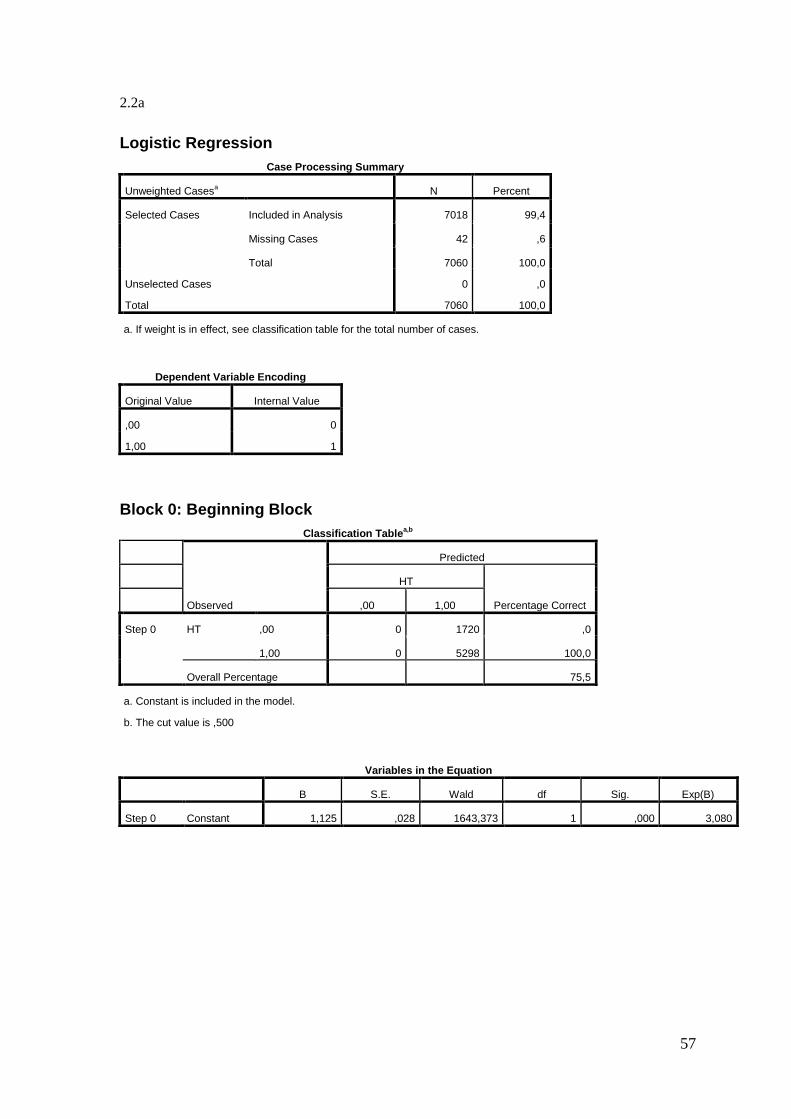
57
2.2a
Logistic Regression
Case Processing Summary
Unweighted Casesa N Percent
Selected Cases Included in Analysis 7018 99,4
Missing Cases 42 ,6
Total 7060 100,0
Unselected Cases 0 ,0
Total 7060 100,0
a. If weight is in effect, see classification table for the total number of cases.
Dependent Variable Encoding
Original Value Internal Value
,00 0
1,00 1
Block 0: Beginning Block
Classification Tablea,b
Observed
Predicted
HT
Percentage Correct
,00 1,00
Step 0 HT ,00 0 1720 ,0
1,00 0 5298 100,0
Overall Percentage 75,5
a. Constant is included in the model.
b. The cut value is ,500
Variables in the Equation
B S.E. Wald df Sig. Exp(B)
Step 0 Constant 1,125 ,028 1643,373 1 ,000 3,080

58
Variables not in the Equation
Score df Sig.
Step 0 Variables Gender 21,321 1 ,000
Age 2,871 1 ,090
Householdsize ,460 1 ,498
Unemployed 142,092 1 ,000
Austria 105,480 1 ,000
Germany 10,476 1 ,001
Sweden ,227 1 ,634
Netherlands 8,042 1 ,005
Spain 67,258 1 ,000
Italy 12,093 1 ,001
France 3,037 1 ,081
Denmark 25,816 1 ,000
Switzerland 143,703 1 ,000
CzechRepublic 8,590 1 ,003
Poland 10,346 1 ,001
Overall Statistics 568,681 15 ,000
Block 1: Method = Enter
Omnibus Tests of Model Coefficients
Chi-square df Sig.
Step 1 Step 567,465 15 ,000
Block 567,465 15 ,000
Model 567,465 15 ,000
Model Summary
Step -2 Log likelihood
Cox & Snell R
Square Nagelkerke R Square
1 7248,758a ,078 ,116
a. Estimation terminated at iteration number 5 because parameter estimates
changed by less than ,001.
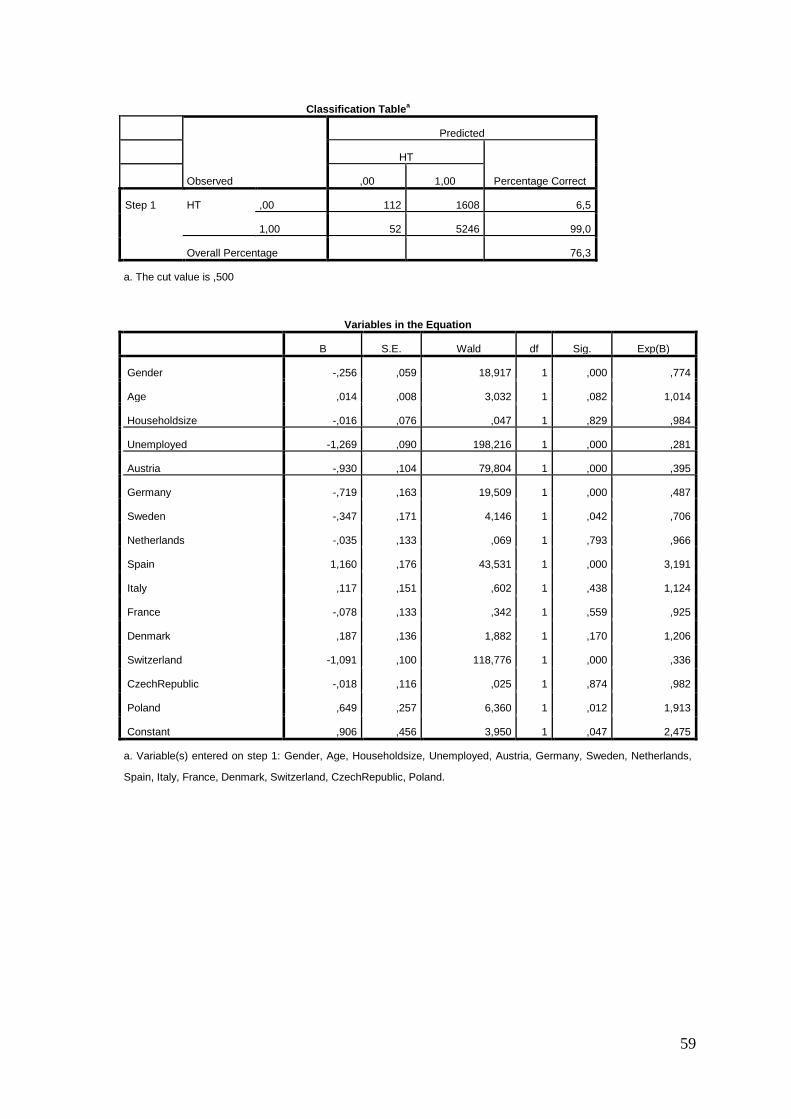
59
Classification Tablea
Observed
Predicted
HT
Percentage Correct
,00 1,00
Step 1 HT ,00 112 1608 6,5
1,00 52 5246 99,0
Overall Percentage 76,3
a. The cut value is ,500
Variables in the Equation
B S.E. Wald df Sig. Exp(B)
Gender -,256 ,059 18,917 1 ,000 ,774
Age ,014 ,008 3,032 1 ,082 1,014
Householdsize -,016 ,076 ,047 1 ,829 ,984
Unemployed -1,269 ,090 198,216 1 ,000 ,281
Austria -,930 ,104 79,804 1 ,000 ,395
Germany -,719 ,163 19,509 1 ,000 ,487
Sweden -,347 ,171 4,146 1 ,042 ,706
Netherlands -,035 ,133 ,069 1 ,793 ,966
Spain 1,160 ,176 43,531 1 ,000 3,191
Italy ,117 ,151 ,602 1 ,438 1,124
France -,078 ,133 ,342 1 ,559 ,925
Denmark ,187 ,136 1,882 1 ,170 1,206
Switzerland -1,091 ,100 118,776 1 ,000 ,336
CzechRepublic -,018 ,116 ,025 1 ,874 ,982
Poland ,649 ,257 6,360 1 ,012 1,913
Constant ,906 ,456 3,950 1 ,047 2,475
a. Variable(s) entered on step 1: Gender, Age, Householdsize, Unemployed, Austria, Germany, Sweden, Netherlands,
Spain, Italy, France, Denmark, Switzerland, CzechRepublic, Poland.

60
2.3a
Logistic Regression
Case Processing Summary
Unweighted Casesa N Percent
Selected Cases Included in Analysis 2240 31,7
Missing Cases 4820 68,3
Total 7060 100,0
Unselected Cases 0 ,0
Total 7060 100,0
a. If weight is in effect, see classification table for the total number of cases.
Dependent Variable Encoding
Original Value Internal Value
,00 0
1,00 1
Block 0: Beginning Block
Classification Tablea,b
Observed
Predicted
HT
Percentage Correct
,00 1,00
Step 0 HT ,00 0 471 ,0
1,00 0 1769 100,0
Overall Percentage 79,0
a. Constant is included in the model.
b. The cut value is ,500
Variables in the Equation
B S.E. Wald df Sig. Exp(B)
Step 0 Constant 1,323 ,052 651,366 1 ,000 3,756

61
Variables not in the Equation
Score df Sig.
Step 0 Variables Gender 17,508 1 ,000
Age ,383 1 ,536
Householdsize ,328 1 ,567
Unemployment_t_1 25,147 1 ,000
Austria 1,219 1 ,270
Germany 16,761 1 ,000
Sweden 2,428 1 ,119
Netherlands ,839 1 ,360
Spain 10,935 1 ,001
Italy 4,560 1 ,033
France ,973 1 ,324
Denmark 8,261 1 ,004
Switzerland 73,962 1 ,000
CzechRepublic 3,965 1 ,046
Poland 7,494 1 ,006
Overall Statistics 174,232 15 ,000
Omnibus Tests of Model Coefficients
Chi-square df Sig.
Step 1 Step 166,898 15 ,000
Block 166,898 15 ,000
Model 166,898 15 ,000
Model Summary
Step -2 Log likelihood
Cox & Snell R
Square Nagelkerke R Square
1 2137,216a ,072 ,112
a. Estimation terminated at iteration number 5 because parameter estimates
changed by less than ,001.
Classification Tablea
Observed
Predicted
HT
Percentage Correct
,00 1,00
Step 1 HT ,00 20 451 4,2
1,00 16 1753 99,1
Overall Percentage 79,2

62
Variables in the Equation
B S.E. Wald df Sig. Exp(B)
Gender -,411 ,111 13,709 1 ,000 ,663
Age ,003 ,019 ,020 1 ,888 1,003
Householdsize ,009 ,141 ,004 1 ,950 1,009
Unemployment_t_1 -1,137 ,192 35,214 1 ,000 ,321
Austria -1,107 ,427 6,727 1 ,009 ,331
Germany -1,139 ,248 21,089 1 ,000 ,320
Sweden -,916 ,255 12,893 1 ,000 ,400
Netherlands -,554 ,258 4,618 1 ,032 ,575
Spain ,297 ,344 ,746 1 ,388 1,346
Italy -,218 ,311 ,489 1 ,484 ,804
France -,751 ,245 9,360 1 ,002 ,472
Denmark -,280 ,249 1,261 1 ,261 ,756
Switzerland -1,781 ,239 55,323 1 ,000 ,168
CzechRepublic -,084 ,322 ,068 1 ,795 ,920
Poland ,273 ,347 ,618 1 ,432 1,314
Constant 2,114 1,130 3,500 1 ,061 8,284
a. Variable(s) entered on step 1: Gender, Age, Householdsize, Unemployment_t_1, Austria, Germany, Sweden,
Netherlands, Spain, Italy, France, Denmark, Switzerland, CzechRepublic, Poland.

63
2.4a
Logistic Regression
Case Processing Summary
Unweighted Casesa N Percent
Selected Cases Included in Analysis 421 6,0
Missing Cases 6639 94,0
Total 7060 100,0
Unselected Cases 0 ,0
Total 7060 100,0
a. If weight is in effect, see classification table for the total number of cases.
Dependent Variable Encoding
Original Value Internal Value
,00 0
1,00 1
Block 0: Beginning Block
Classification Tablea,b
Observed
Predicted
HT
Percentage Correct
,00 1,00
Step 0 HT ,00 0 206 ,0
1,00 0 215 100,0
Overall Percentage 51,1
a. Constant is included in the model.
b. The cut value is ,500
Variables in the Equation
B S.E. Wald df Sig. Exp(B)
Step 0 Constant ,043 ,097 ,192 1 ,661 1,044

64
Variables not in the Equation
Score df Sig.
Step 0 Variables Gender ,280 1 ,597
Age 13,546 1 ,000
Householdsize ,982 1 ,322
LongtermUnemployment 2,364 1 ,124
Austria 9,502 1 ,002
Netherlands ,032 1 ,858
Spain 36,381 1 ,000
Italy 1,012 1 ,314
France 1,225 1 ,268
Denmark 5,264 1 ,022
Switzerland 13,469 1 ,000
CzechRepublic ,914 1 ,339
Overall Statistics 75,890 12 ,000
Block 1: Method = Enter
Omnibus Tests of Model Coefficients
Chi-square df Sig.
Step 1 Step 83,597 12 ,000
Block 83,597 12 ,000
Model 83,597 12 ,000
Model Summary
Step -2 Log likelihood
Cox & Snell R
Square
Nagelkerke R
Square
1 499,841a ,180 ,240
a. Estimation terminated at iteration number 5 because parameter estimates
changed by less than ,001.

65
Classification Tablea
Observed
Predicted
HT
Percentage Correct
,00 1,00
Step 1 HT ,00 143 63 69,4
1,00 75 140 65,1
Overall Percentage 67,2
a. The cut value is ,500
Variables in the Equation
B S.E. Wald df Sig. Exp(B)
Gender ,091 ,221 ,169 1 ,681 1,095
Age ,131 ,033 15,885 1 ,000 1,140
Householdsize ,084 ,293 ,082 1 ,775 1,087
LongtermUnemployment -,500 ,235 4,517 1 ,034 ,606
Austria -,309 ,310 ,999 1 ,318 ,734
Netherlands ,467 ,579 ,649 1 ,421 1,594
Spain 1,747 ,354 24,284 1 ,000 5,736
Italy ,956 ,615 2,413 1 ,120 2,602
France -,096 ,566 ,029 1 ,865 ,908
Denmark 2,464 1,103 4,990 1 ,025 11,757
Switzerland -1,243 ,515 5,822 1 ,016 ,288
CzechRepublic ,538 ,346 2,418 1 ,120 1,712
Constant -7,278 1,837 15,689 1 ,000 ,001
a. Variable(s) entered on step 1: Gender, Age, Householdsize, LongtermUnemployment, Austria, Netherlands, Spain,
Italy, France, Denmark, Switzerland, CzechRepublic.
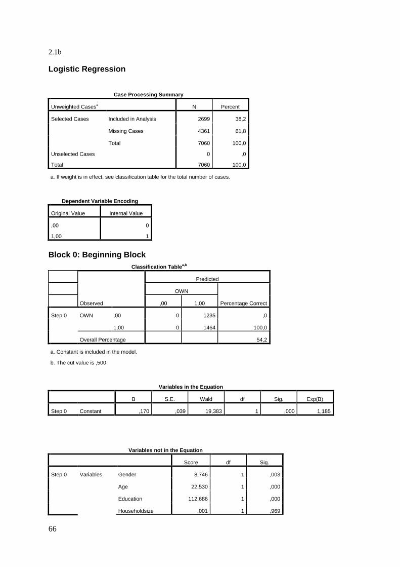
66
2.1b
Logistic Regression
Case Processing Summary
Unweighted Casesa N Percent
Selected Cases Included in Analysis 2699 38,2
Missing Cases 4361 61,8
Total 7060 100,0
Unselected Cases 0 ,0
Total 7060 100,0
a. If weight is in effect, see classification table for the total number of cases.
Dependent Variable Encoding
Original Value Internal Value
,00 0
1,00 1
Block 0: Beginning Block
Classification Tablea,b
Observed
Predicted
OWN
Percentage Correct
,00 1,00
Step 0 OWN ,00 0 1235 ,0
1,00 0 1464 100,0
Overall Percentage 54,2
a. Constant is included in the model.
b. The cut value is ,500
Variables in the Equation
B S.E. Wald df Sig. Exp(B)
Step 0 Constant ,170 ,039 19,383 1 ,000 1,185
Variables not in the Equation
Score df Sig.
Step 0 Variables Gender 8,746 1 ,003
Age 22,530 1 ,000
Education 112,686 1 ,000
Householdsize ,001 1 ,969
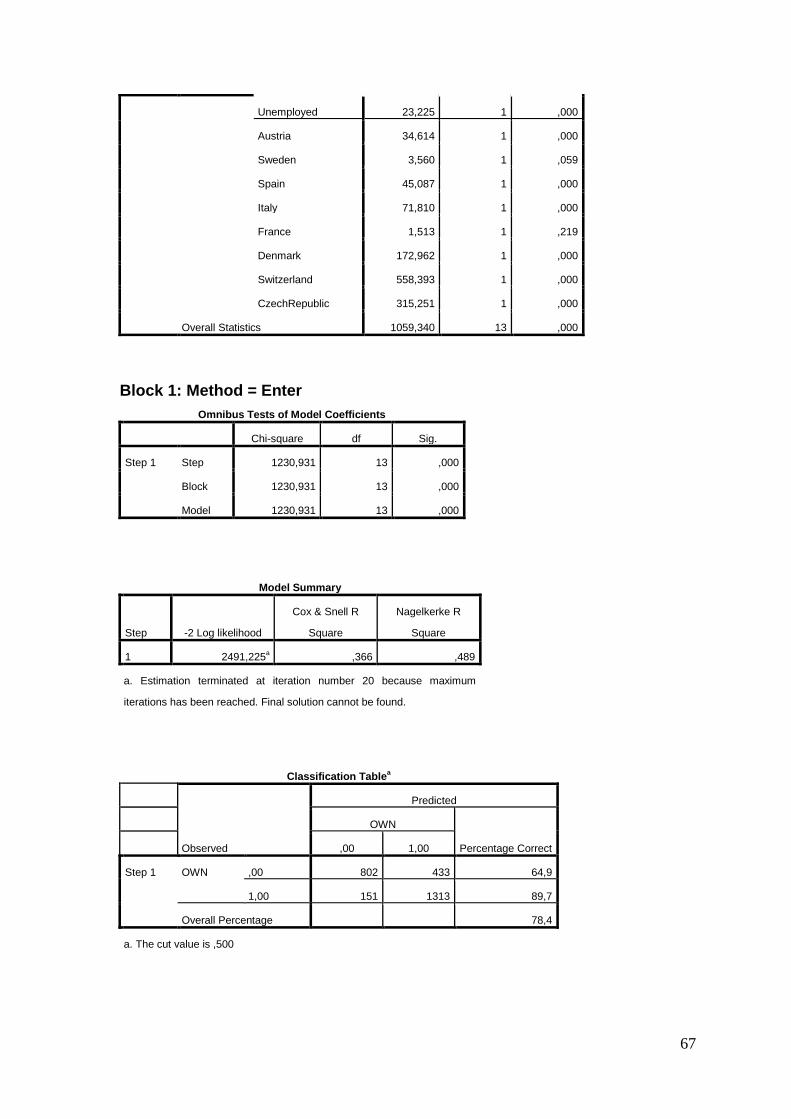
67
Unemployed 23,225 1 ,000
Austria 34,614 1 ,000
Sweden 3,560 1 ,059
Spain 45,087 1 ,000
Italy 71,810 1 ,000
France 1,513 1 ,219
Denmark 172,962 1 ,000
Switzerland 558,393 1 ,000
CzechRepublic 315,251 1 ,000
Overall Statistics 1059,340 13 ,000
Block 1: Method = Enter
Omnibus Tests of Model Coefficients
Chi-square df Sig.
Step 1 Step 1230,931 13 ,000
Block 1230,931 13 ,000
Model 1230,931 13 ,000
Model Summary
Step -2 Log likelihood
Cox & Snell R
Square
Nagelkerke R
Square
1 2491,225a ,366 ,489
a. Estimation terminated at iteration number 20 because maximum
iterations has been reached. Final solution cannot be found.
Classification Tablea
Observed
Predicted
OWN
Percentage Correct
,00 1,00
Step 1 OWN ,00 802 433 64,9
1,00 151 1313 89,7
Overall Percentage 78,4
a. The cut value is ,500

68
Variables in the Equation
B S.E. Wald df Sig. Exp(B)
Step 1a Gender ,129 ,101 1,636 1 ,201 1,138
Age ,095 ,015 40,490 1 ,000 1,099
Education -,069 ,113 ,370 1 ,543 ,933
Householdsize ,080 ,132 ,363 1 ,547 1,083
Unemployed ,274 ,199 1,885 1 ,170 1,315
Austria ,977 ,150 42,136 1 ,000 2,656
Sweden -21,197 22795,050 ,000 1 ,999 ,000
Spain 1,161 ,176 43,329 1 ,000 3,193
Italy 1,775 ,213 69,754 1 ,000 5,902
France ,786 ,196 16,038 1 ,000 2,195
Denmark -1,746 ,266 43,134 1 ,000 ,174
Switzerland -2,842 ,247 131,881 1 ,000 ,058
CzechRepublic 2,347 ,178 174,127 1 ,000 10,450
Constant -5,492 ,828 43,979 1 ,000 ,004
a. Variable(s) entered on step 1: Gender, Age, Education, Householdsize, Unemployed, Austria, Sweden, Spain, Italy, France,
Denmark, Switzerland, CzechRepublic.
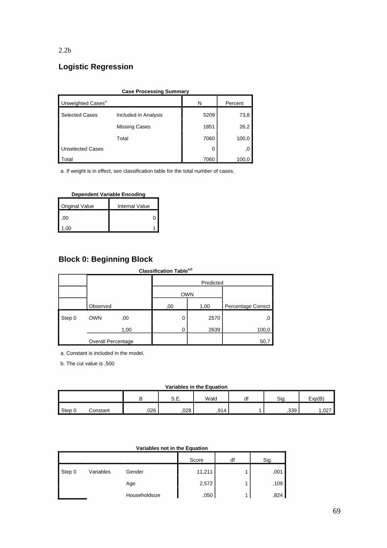
69
2.2b
Logistic Regression
Case Processing Summary
Unweighted Casesa N Percent
Selected Cases Included in Analysis 5209 73,8
Missing Cases 1851 26,2
Total 7060 100,0
Unselected Cases 0 ,0
Total 7060 100,0
a. If weight is in effect, see classification table for the total number of cases.
Dependent Variable Encoding
Original Value Internal Value
,00 0
1,00 1
Block 0: Beginning Block
Classification Tablea,b
Observed
Predicted
OWN
Percentage Correct
,00 1,00
Step 0 OWN ,00 0 2570 ,0
1,00 0 2639 100,0
Overall Percentage 50,7
a. Constant is included in the model.
b. The cut value is ,500
Variables in the Equation
B S.E. Wald df Sig. Exp(B)
Step 0 Constant ,026 ,028 ,914 1 ,339 1,027
Variables not in the Equation
Score df Sig.
Step 0 Variables Gender 11,211 1 ,001
Age 2,572 1 ,109
Householdsize ,050 1 ,824

70
Unemployed 46,011 1 ,000
Austria 54,754 1 ,000
Germany 4,900 1 ,027
Sweden 84,980 1 ,000
Netherlands 335,570 1 ,000
Spain 105,823 1 ,000
Italy 142,403 1 ,000
France 41,970 1 ,000
Denmark 297,249 1 ,000
Switzerland 554,055 1 ,000
CzechRepublic 435,170 1 ,000
Poland 99,471 1 ,000
Overall Statistics 2012,297 15 ,000
Block 1: Method = Enter
Omnibus Tests of Model Coefficients
Chi-square df Sig.
Step 1 Step 2326,285 15 ,000
Block 2326,285 15 ,000
Model 2326,285 15 ,000
Model Summary
Step -2 Log likelihood
Cox & Snell R
Square
Nagelkerke R
Square
1 4894,008a ,360 ,480
a. Estimation terminated at iteration number 5 because parameter
estimates changed by less than ,001.

71
Classification Tablea
Observed
Predicted
OWN
Percentage Correct
,00 1,00
Step 1 OWN ,00 1745 825 67,9
1,00 329 2310 87,5
Overall Percentage 77,8
a. The cut value is ,500
Variables in the Equation
B S.E. Wald df Sig. Exp(B)
Step 1a Gender ,124 ,072 2,962 1 ,085 1,132
Age ,090 ,010 78,400 1 ,000 1,094
Householdsize ,051 ,092 ,308 1 ,579 1,053
Unemployed ,291 ,139 4,357 1 ,037 1,337
Austria ,568 ,117 23,395 1 ,000 1,765
Germany -,103 ,183 ,315 1 ,574 ,902
Sweden -2,085 ,204 104,616 1 ,000 ,124
Netherlands -2,756 ,192 207,042 1 ,000 ,064
Spain ,795 ,132 36,058 1 ,000 2,213
Italy 1,347 ,159 71,514 1 ,000 3,845
France ,506 ,128 15,699 1 ,000 1,658
Denmark -2,117 ,150 200,542 1 ,000 ,120
Switzerland -3,093 ,189 266,886 1 ,000 ,045
CzechRepublic 1,980 ,146 183,866 1 ,000 7,246
Poland 2,415 ,372 42,065 1 ,000 11,186
Constant -4,882 ,569 73,606 1 ,000 ,008
a. Variable(s) entered on step 1: Gender, Age, Householdsize, Unemployed, Austria, Germany, Sweden, Netherlands, Spain,
Italy, France, Denmark, Switzerland, CzechRepublic, Poland.

72
2.3b
Logistic Regression
Case Processing Summary
Unweighted Casesa N Percent
Selected Cases Included in Analysis 1742 24,7
Missing Cases 5318 75,3
Total 7060 100,0
Unselected Cases 0 ,0
Total 7060 100,0
a. If weight is in effect, see classification table for the total number of cases.
Dependent Variable Encoding
Original Value Internal Value
,00 0
1,00 1
Block 0: Beginning Block
Classification Tablea,b
Observed
Predicted
OWN
Percentage Correct
,00 1,00
Step 0 OWN ,00 882 0 100,0
1,00 860 0 ,0
Overall Percentage 50,6
a. Constant is included in the model.
b. The cut value is ,500
Variables in the Equation
B S.E. Wald df Sig. Exp(B)
Step 0 Constant -,025 ,048 ,278 1 ,598 ,975

73
Variables not in the Equation
Score df Sig.
Step 0 Variables Gender ,887 1 ,346
Age 9,760 1 ,002
Householdsize ,003 1 ,960
Austria ,446 1 ,504
Germany 5,938 1 ,015
Sweden 61,124 1 ,000
Netherlands 125,347 1 ,000
Spain 42,332 1 ,000
Italy 54,594 1 ,000
France 39,774 1 ,000
Denmark 146,600 1 ,000
Switzerland 80,965 1 ,000
CzechRepublic 84,644 1 ,000
Poland 92,051 1 ,000
Unemployment_t_1 20,208 1 ,000
Overall Statistics 690,823 15 ,000
Block 1: Method = Enter
Omnibus Tests of Model Coefficients
Chi-square df Sig.
Step 1 Step 776,527 15 ,000
Block 776,527 15 ,000
Model 776,527 15 ,000
Model Summary
Step -2 Log likelihood
Cox & Snell R
Square
Nagelkerke R
Square
1 1638,120a ,360 ,480
a. Estimation terminated at iteration number 5 because parameter
estimates changed by less than ,001.
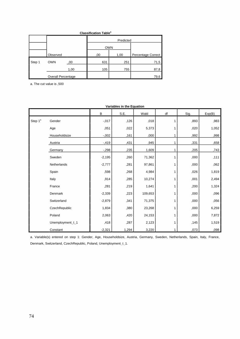
74
Classification Tablea
Observed
Predicted
OWN
Percentage Correct
,00 1,00
Step 1 OWN ,00 631 251 71,5
1,00 105 755 87,8
Overall Percentage 79,6
a. The cut value is ,500
Variables in the Equation
B S.E. Wald df Sig. Exp(B)
Step 1a Gender -,017 ,126 ,018 1 ,893 ,983
Age ,051 ,022 5,373 1 ,020 1,052
Householdsize -,002 ,161 ,000 1 ,992 ,998
Austria -,419 ,431 ,945 1 ,331 ,658
Germany -,298 ,235 1,609 1 ,205 ,743
Sweden -2,195 ,260 71,362 1 ,000 ,111
Netherlands -2,777 ,281 97,861 1 ,000 ,062
Spain ,598 ,268 4,984 1 ,026 1,819
Italy ,914 ,285 10,274 1 ,001 2,494
France ,281 ,219 1,641 1 ,200 1,324
Denmark -2,339 ,223 109,653 1 ,000 ,096
Switzerland -2,879 ,341 71,375 1 ,000 ,056
CzechRepublic 1,834 ,380 23,268 1 ,000 6,259
Poland 2,063 ,420 24,153 1 ,000 7,872
Unemployment_t_1 ,418 ,287 2,123 1 ,145 1,519
Constant -2,321 1,294 3,220 1 ,073 ,098
a. Variable(s) entered on step 1: Gender, Age, Householdsize, Austria, Germany, Sweden, Netherlands, Spain, Italy, France,
Denmark, Switzerland, CzechRepublic, Poland, Unemployment_t_1.

75
2.4b
Logistic Regression
Case Processing Summary
Unweighted Casesa N Percent
Selected Cases Included in Analysis 179 2,5
Missing Cases 6881 97,5
Total 7060 100,0
Unselected Cases 0 ,0
Total 7060 100,0
a. If weight is in effect, see classification table for the total number of cases.
Dependent Variable Encoding
Original Value Internal Value
,00 0
1,00 1
Block 0: Beginning Block
Classification Tablea,b
Observed
Predicted
OWN
Percentage Correct
,00 1,00
Step 0 OWN ,00 0 51 ,0
1,00 0 128 100,0
Overall Percentage 71,5
a. Constant is included in the model.
b. The cut value is ,500
Variables in the Equation
B S.E. Wald df Sig. Exp(B)
Step 0 Constant ,920 ,166 30,881 1 ,000 2,510
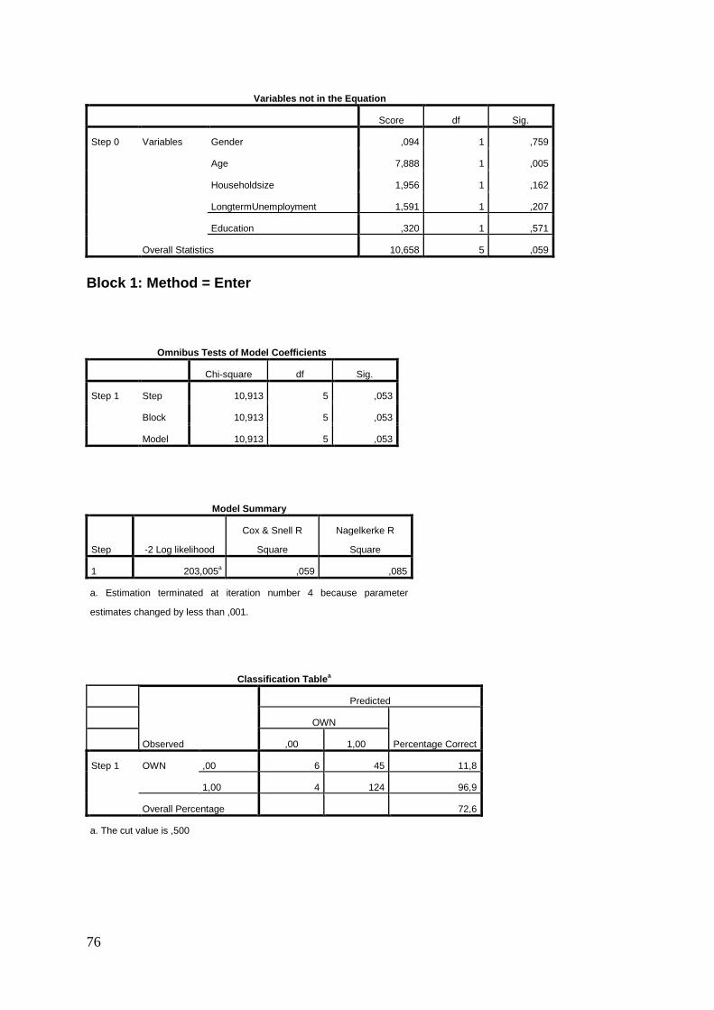
76
Variables not in the Equation
Score df Sig.
Step 0 Variables Gender ,094 1 ,759
Age 7,888 1 ,005
Householdsize 1,956 1 ,162
LongtermUnemployment 1,591 1 ,207
Education ,320 1 ,571
Overall Statistics 10,658 5 ,059
Block 1: Method = Enter
Omnibus Tests of Model Coefficients
Chi-square df Sig.
Step 1 Step 10,913 5 ,053
Block 10,913 5 ,053
Model 10,913 5 ,053
Model Summary
Step -2 Log likelihood
Cox & Snell R
Square
Nagelkerke R
Square
1 203,005a ,059 ,085
a. Estimation terminated at iteration number 4 because parameter
estimates changed by less than ,001.
Classification Tablea
Observed
Predicted
OWN
Percentage Correct
,00 1,00
Step 1 OWN ,00 6 45 11,8
1,00 4 124 96,9
Overall Percentage 72,6
a. The cut value is ,500

77
Variables in the Equation
B S.E. Wald df Sig. Exp(B)
Gender -,068 ,348 ,038 1 ,845 ,934
Age ,128 ,049 6,974 1 ,008 1,137
Householdsize -,623 ,418 2,221 1 ,136 ,536
LongtermUnemployment ,232 ,352 ,433 1 ,510 1,261
Education -,039 ,361 ,012 1 ,914 ,962
Constant -6,143 2,682 5,245 1 ,022 ,002
a. Variable(s) entered on step 1: Gender, Age, Householdsize, LongtermUnemployment, Education.
SPSS Output RQ3
3.1
Regression
Descriptive Statistics
Mean Std. Deviation N
Log_Financial_Assets_PPP 8,7866 2,47440 4482
HT ,7320 ,44295 4482
AGE 63,9630 10,15174 4482
GN ,5455 ,49798 4482
EDU ,5315 ,49907 4482
MAR ,6466 ,47808 4482
CNAT ,3021 ,45922 4482
CNDE ,0013 ,03657 4482
CNSE ,0009 ,02986 4482
CNNL ,0000 ,00000 4482
CNES ,0754 ,26409 4482
CNIT ,0542 ,22647 4482
CNFR ,1959 ,39693 4482
CNDK ,0366 ,18778 4482
CNCH ,1843 ,38777 4482
CNCZ ,1481 ,35529 4482
CNPL ,0011 ,03339 4482

78
Variables Entered/Removeda
Model Variables Entered Variables Removed Method
1 CNPL, CNSE, CNDE,
CNDK, CNIT, GN,
CNES, HT, AGE,
CNCZ, CNCH, MAR,
EDU, CNFRb
. Enter
a. Dependent Variable: Log_Financial_Assets_PPP
b. Tolerance = ,000 limit reached.
Model Summary
Model R R Square Adjusted R Square
Std. Error of the
Estimate
1 ,483a ,233 ,230 2,17066
a. Predictors: (Constant), CNPL, CNSE, CNDE, CNDK, CNIT, GN, CNES, HT, AGE, CNCZ,
CNCH, MAR, EDU, CNFR
ANOVAa
Model Sum of Squares df Mean Square F Sig.
1 Regression 6388,272 14 456,305 96,844 ,000b
Residual 21047,379 4467 4,712
Total 27435,652 4481
a. Dependent Variable: Log_Financial_Assets_PPP
b. Predictors: (Constant), CNPL, CNSE, CNDE, CNDK, CNIT, GN, CNES, HT, AGE, CNCZ, CNCH, MAR, EDU, CNFR
Coefficientsa
Model
Unstandardized Coefficients Standardized Coefficients
t Sig.
Collinearity Statistics
B Std. Error Beta Tolerance VIF
(Constant) 6,717 ,256 26,208 ,000
HT ,775 ,078 ,139 9,986 ,000 ,889 1,125
AGE ,006 ,003 ,025 1,802 ,072 ,897 1,115
GN -,431 ,069 -,087 -6,289 ,000 ,904 1,107
EDU ,733 ,079 ,148 9,295 ,000 ,679 1,473
MAR ,485 ,074 ,094 6,560 ,000 ,840 1,191
CNDE 1,352 ,889 ,020 1,521 ,128 ,994 1,006

79
CNSE 1,848 1,088 ,022 1,699 ,089 ,997 1,003
CNES -,328 ,141 -,035 -2,320 ,020 ,756 1,323
CNIT ,284 ,160 ,026 1,779 ,075 ,804 1,244
CNFR 1,003 ,102 ,161 9,862 ,000 ,645 1,550
CNDK 1,397 ,185 ,106 7,560 ,000 ,874 1,145
CNCH 2,267 ,098 ,355 23,221 ,000 ,734 1,363
CNCZ -,102 ,104 -,015 -,980 ,327 ,771 1,298
CNPL ,370 ,974 ,005 ,380 ,704 ,995 1,005
a. Dependent Variable: Log_Financial_Assets_PPP
Excluded Variablesa
Model Beta In t Sig. Partial Correlation
Collinearity Statistics
Tolerance VIF Minimum Tolerance
1 CNAT .b . . . -6,240E-14
-
16024754644380,553 -6,240E-14
a. Dependent Variable: Log_Financial_Assets_PPP
b. Predictors in the Model: (Constant), CNPL, CNSE, CNDE, CNDK, CNIT, GN, CNES, HT, AGE, CNCZ, CNCH, MAR, EDU, CNFR
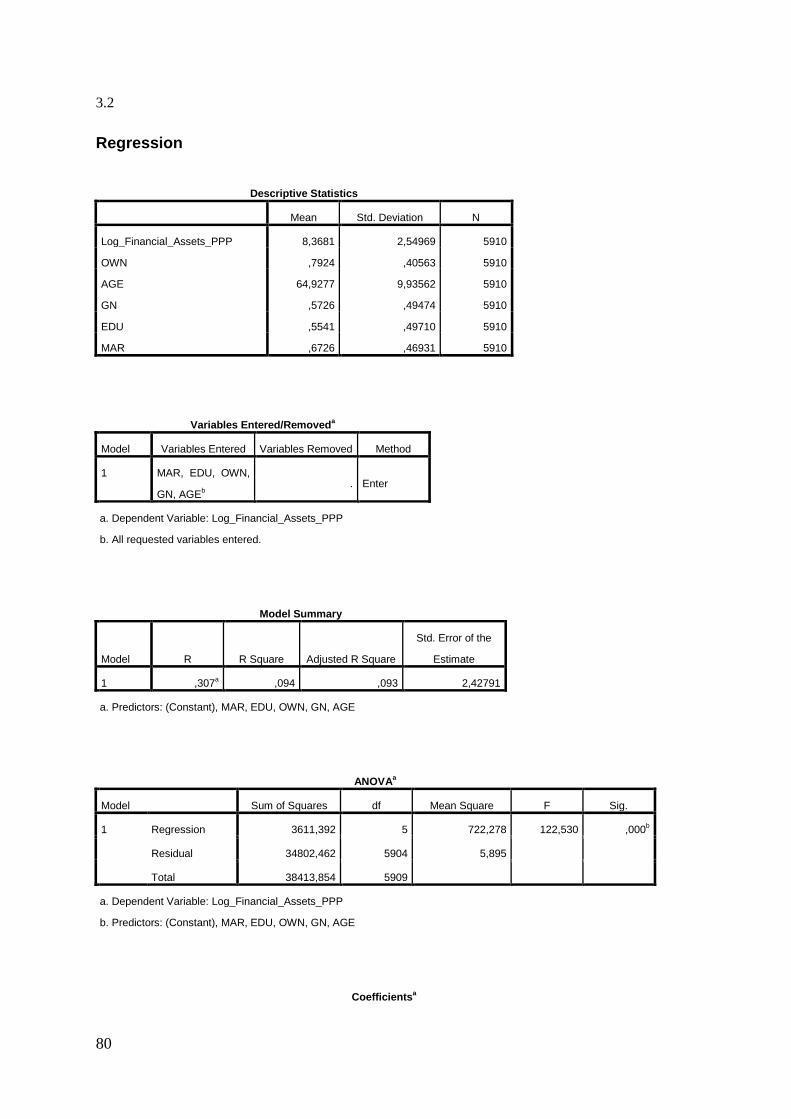
80
3.2
Regression
Descriptive Statistics
Mean Std. Deviation N
Log_Financial_Assets_PPP 8,3681 2,54969 5910
OWN ,7924 ,40563 5910
AGE 64,9277 9,93562 5910
GN ,5726 ,49474 5910
EDU ,5541 ,49710 5910
MAR ,6726 ,46931 5910
Variables Entered/Removeda
Model Variables Entered Variables Removed Method
1 MAR, EDU, OWN,
GN, AGEb
. Enter
a. Dependent Variable: Log_Financial_Assets_PPP
b. All requested variables entered.
Model Summary
Model R R Square Adjusted R Square
Std. Error of the
Estimate
1 ,307a ,094 ,093 2,42791
a. Predictors: (Constant), MAR, EDU, OWN, GN, AGE
ANOVAa
Model Sum of Squares df Mean Square F Sig.
1 Regression 3611,392 5 722,278 122,530 ,000b
Residual 34802,462 5904 5,895
Total 38413,854 5909
a. Dependent Variable: Log_Financial_Assets_PPP
b. Predictors: (Constant), MAR, EDU, OWN, GN, AGE
Coefficientsa

81
Model
Unstandardized Coefficients
Standardized
Coefficients
t Sig.
Collinearity Statistics
B Std. Error Beta Tolerance VIF
1 (Constant) 8,996 ,243 36,984 ,000
OWN -1,246 ,082 -,198 -15,206 ,000 ,903 1,107
AGE ,004 ,003 ,015 1,095 ,273 ,874 1,144
GN -,767 ,066 -,149 -11,596 ,000 ,931 1,075
EDU ,378 ,064 ,074 5,896 ,000 ,981 1,020
MAR ,516 ,072 ,095 7,199 ,000 ,882 1,134
a. Dependent Variable: Log_Financial_Assets_PPP

82
3.2bis
Regression
Descriptive Statistics
Mean Std. Deviation N
Log_Financial_Assets_PPP 8,9777 2,43227 3342
OWN ,7142 ,45184 3342
AGE 63,9928 10,05429 3342
GN ,5272 ,49933 3342
EDU ,5239 ,49950 3342
MAR ,7050 ,45613 3342
CNAT ,2501 ,43316 3342
CNDE ,0018 ,04234 3342
CNSE ,0018 ,04234 3342
CNNL ,0000 ,00000 3342
CNES ,0910 ,28760 3342
CNIT ,0640 ,24485 3342
CNFR ,2059 ,40439 3342
CNDK ,0413 ,19900 3342
CNCH ,1562 ,36309 3342
CNCZ ,1867 ,38974 3342
CNPL ,0012 ,03458 3342
Variables Entered/Removeda
Model Variables Entered Variables Removed Method
1 CNPL, CNSE, CNDE,
CNDK, CNIT, GN,
CNES, AGE, CNCH,
MAR, CNCZ, EDU,
CNFR, OWNb
. Enter
a. Dependent Variable: Log_Financial_Assets_PPP
b. Tolerance = ,000 limit reached.
Model Summary

83
Model R R Square Adjusted R Square
Std. Error of the
Estimate
1 ,496a ,246 ,243 2,11671
a. Predictors: (Constant), CNPL, CNSE, CNDE, CNDK, CNIT, GN, CNES, AGE, CNCH, MAR,
CNCZ, EDU, CNFR, OWN
ANOVAa
Model Sum of Squares df Mean Square F Sig.
1 Regression 4858,650 14 347,046 77,457 ,000b
Residual 14906,554 3327 4,480
Total 19765,204 3341
a. Dependent Variable: Log_Financial_Assets_PPP
b. Predictors: (Constant), CNPL, CNSE, CNDE, CNDK, CNIT, GN, CNES, AGE, CNCH, MAR, CNCZ, EDU, CNFR, OWN
Coefficientsa
Model
Unstandardized Coefficients
Standardized
Coefficients
t Sig. B Std. Error Beta
1 (Constant) 7,721 ,304 25,375 ,000
OWN ,127 ,109 ,024 1,160 ,246
AGE ,001 ,004 ,003 ,160 ,873
GN -,511 ,077 -,105 -6,630 ,000
EDU ,742 ,089 ,152 8,290 ,000
MAR ,330 ,086 ,062 3,858 ,000
CNDE 1,458 ,868 ,025 1,679 ,093
CNSE 2,323 ,870 ,040 2,670 ,008
CNES -,069 ,150 -,008 -,458 ,647
CNIT ,438 ,171 ,044 2,569 ,010
CNFR 1,284 ,116 ,213 11,096 ,000
CNDK 1,781 ,210 ,146 8,463 ,000
CNCH 2,664 ,141 ,398 18,834 ,000
CNCZ -,057 ,113 -,009 -,506 ,613
CNPL ,354 1,062 ,005 ,333 ,739
a. Dependent Variable: Log_Financial_Assets_PPP

84
Excluded Variablesa
Model Beta In t Sig. Partial Correlation
Collinearity Statistics
Tolerance
1 CNAT .b . . . ,000
a. Dependent Variable: Log_Financial_Assets_PPP
b. Predictors in the Model: (Constant), CNPL, CNSE, CNDE, CNDK, CNIT, GN, CNES, AGE, CNCH, MAR, CNCZ, EDU,
CNFR, OWN
3.3
Regression
Descriptive Statistics
Mean Std. Deviation N
Log_Financial_Assets_PPP 9,6735 2,15384 456
HOUSEXP ,2590 ,19806 456
AGE 54,9715 4,45604 456
GN ,4474 ,49777 456
EDU ,6864 ,46446 456
MAR ,7675 ,42286 456
Variables Entered/Removeda
Model Variables Entered Variables Removed Method
1 MAR, AGE, EDU,
GN, HOUSEXPb
. Enter
a. Dependent Variable: Log_Financial_Assets_PPP
b. All requested variables entered.
Model Summary
Model R R Square Adjusted R Square
Std. Error of the
Estimate
1 ,358a ,128 ,118 2,02239
a. Predictors: (Constant), MAR, AGE, EDU, GN, HOUSEXP
ANOVAa
Model Sum of Squares df Mean Square F Sig.

85
1 Regression 270,223 5 54,045 13,214 ,000b
Residual 1840,530 450 4,090
Total 2110,753 455
a. Dependent Variable: Log_Financial_Assets_PPP
b. Predictors: (Constant), MAR, AGE, EDU, GN, HOUSEXP
Coefficientsa
Model
Unstandardized Coefficients
Standardized
Coefficients
t Sig. B Std. Error Beta
1 (Constant) 7,241 1,265 5,725 ,000
HOUSEXP -1,109 ,508 -,102 -2,185 ,029
AGE ,027 ,022 ,056 1,258 ,209
GN -,254 ,201 -,059 -1,261 ,208
EDU 1,274 ,210 ,275 6,083 ,000
MAR ,604 ,228 ,119 2,646 ,008
a. Dependent Variable: Log_Financial_Assets_PPP
3.4
Regression
Descriptive Statistics
Mean Std. Deviation N
w ,4451 ,29778 874
HT ,8146 ,38881 874
AGE 63,3844 9,83348 874
GN ,3959 ,48932 874
EDU ,7277 ,44540 874
MAR ,7586 ,42819 874
CNAT ,2002 ,40040 874
CNDE ,0023 ,04781 874
CNSE ,0034 ,05852 874
CNNL ,0000 ,00000 874
CNES ,0297 ,16999 874
CNIT ,0584 ,23454 874
CNFR ,1739 ,37925 874
CNDK ,0950 ,29334 874
CNCH ,3684 ,48265 874
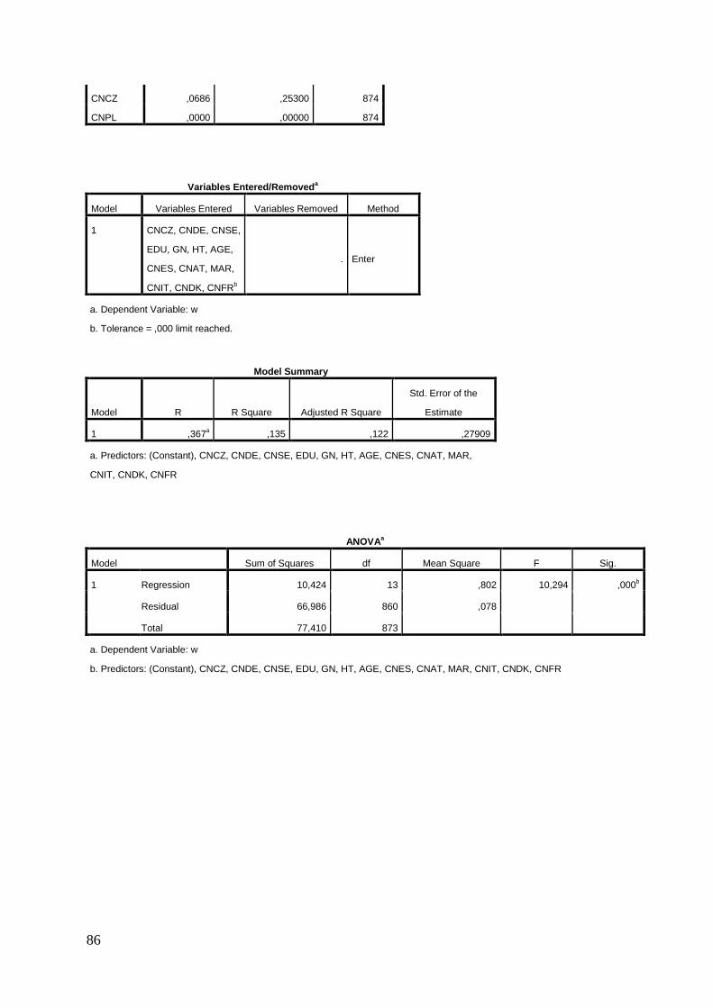
86
CNCZ ,0686 ,25300 874
CNPL ,0000 ,00000 874
Variables Entered/Removeda
Model Variables Entered Variables Removed Method
1 CNCZ, CNDE, CNSE,
EDU, GN, HT, AGE,
CNES, CNAT, MAR,
CNIT, CNDK, CNFRb
. Enter
a. Dependent Variable: w
b. Tolerance = ,000 limit reached.
Model Summary
Model R R Square Adjusted R Square
Std. Error of the
Estimate
1 ,367a ,135 ,122 ,27909
a. Predictors: (Constant), CNCZ, CNDE, CNSE, EDU, GN, HT, AGE, CNES, CNAT, MAR,
CNIT, CNDK, CNFR
ANOVAa
Model Sum of Squares df Mean Square F Sig.
1 Regression 10,424 13 ,802 10,294 ,000b
Residual 66,986 860 ,078
Total 77,410 873
a. Dependent Variable: w
b. Predictors: (Constant), CNCZ, CNDE, CNSE, EDU, GN, HT, AGE, CNES, CNAT, MAR, CNIT, CNDK, CNFR
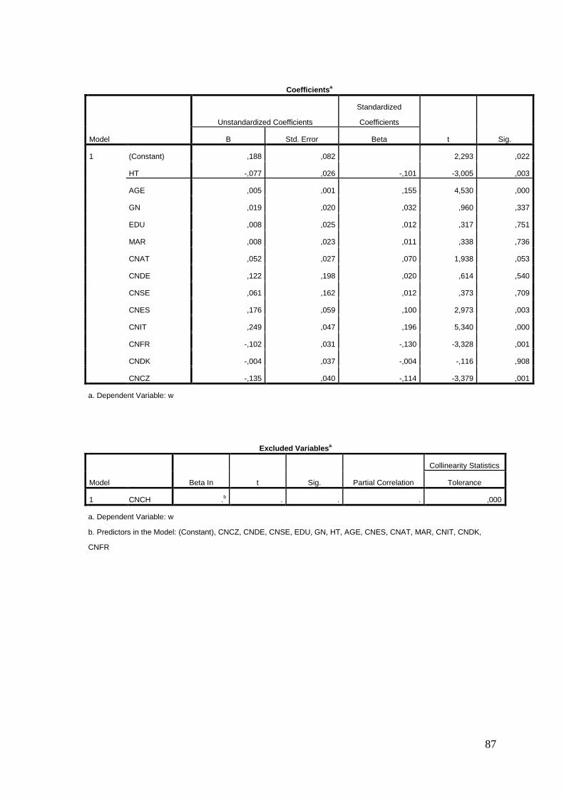
87
Coefficientsa
Model
Unstandardized Coefficients
Standardized
Coefficients
t Sig. B Std. Error Beta
1 (Constant) ,188 ,082 2,293 ,022
HT -,077 ,026 -,101 -3,005 ,003
AGE ,005 ,001 ,155 4,530 ,000
GN ,019 ,020 ,032 ,960 ,337
EDU ,008 ,025 ,012 ,317 ,751
MAR ,008 ,023 ,011 ,338 ,736
CNAT ,052 ,027 ,070 1,938 ,053
CNDE ,122 ,198 ,020 ,614 ,540
CNSE ,061 ,162 ,012 ,373 ,709
CNES ,176 ,059 ,100 2,973 ,003
CNIT ,249 ,047 ,196 5,340 ,000
CNFR -,102 ,031 -,130 -3,328 ,001
CNDK -,004 ,037 -,004 -,116 ,908
CNCZ -,135 ,040 -,114 -3,379 ,001
a. Dependent Variable: w
Excluded Variablesa
Model Beta In t Sig. Partial Correlation
Collinearity Statistics
Tolerance
1 CNCH .b . . . ,000
a. Dependent Variable: w
b. Predictors in the Model: (Constant), CNCZ, CNDE, CNSE, EDU, GN, HT, AGE, CNES, CNAT, MAR, CNIT, CNDK,
CNFR
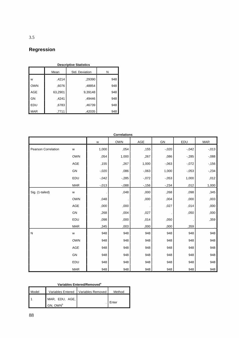
88
3.5
Regression
Descriptive Statistics
Mean Std. Deviation N
w ,4214 ,29390 948
OWN ,6076 ,48854 948
AGE 63,2901 9,39148 948
GN ,4241 ,49446 948
EDU ,6783 ,46739 948
MAR ,7711 ,42035 948
Correlations
w OWN AGE GN EDU MAR
Pearson Correlation w 1,000 ,054 ,155 -,020 -,042 -,013
OWN ,054 1,000 ,267 ,086 -,285 -,088
AGE ,155 ,267 1,000 -,063 -,072 -,156
GN -,020 ,086 -,063 1,000 -,053 -,234
EDU -,042 -,285 -,072 -,053 1,000 ,012
MAR -,013 -,088 -,156 -,234 ,012 1,000
Sig. (1-tailed) w . ,048 ,000 ,268 ,098 ,345
OWN ,048 . ,000 ,004 ,000 ,003
AGE ,000 ,000 . ,027 ,014 ,000
GN ,268 ,004 ,027 . ,050 ,000
EDU ,098 ,000 ,014 ,050 . ,359
MAR ,345 ,003 ,000 ,000 ,359 .
N w 948 948 948 948 948 948
OWN 948 948 948 948 948 948
AGE 948 948 948 948 948 948
GN 948 948 948 948 948 948
EDU 948 948 948 948 948 948
MAR 948 948 948 948 948 948
Variables Entered/Removeda
Model Variables Entered Variables Removed Method
1 MAR, EDU, AGE,
GN, OWNb
. Enter

89
Model Summary
Model R R Square Adjusted R Square
Std. Error of the
Estimate
1 ,159a ,025 ,020 ,29095
a. Predictors: (Constant), MAR, EDU, AGE, GN, OWN
ANOVAa
Model Sum of Squares df Mean Square F Sig.
1 Regression 2,057 5 ,411 4,859 ,000b
Residual 79,743 942 ,085
Total 81,800 947
a. Dependent Variable: w
b. Predictors: (Constant), MAR, EDU, AGE, GN, OWN
Coefficientsa
Model
Unstandardized Coefficients
Standardized
Coefficients
t Sig.
Collinearity Statistics
B Std. Error Beta Tolerance VIF
1 (Constant) ,129 ,075 1,718 ,086
OWN ,004 ,021 ,007 ,204 ,839 ,849 1,177
AGE ,005 ,001 ,151 4,456 ,000 ,897 1,115
GN -,006 ,020 -,011 -,320 ,749 ,925 1,081
EDU -,019 ,021 -,030 -,886 ,376 ,917 1,090
MAR ,006 ,024 ,009 ,272 ,786 ,915 1,093
a. Dependent Variable: w

90
3.6
Regression
Descriptive Statistics
Mean Std. Deviation N
w ,3232 ,26831 111
HOUSEXP ,2134 ,15572 111
AGE 54,8739 4,49468 111
GN ,3243 ,47024 111
EDU ,8829 ,32302 111
MAR ,8739 ,33350 111
CNAT ,0991 ,30015 111
CNDE ,0000 ,00000 111
CNSE ,0090 ,09492 111
CNNL ,0000 ,00000 111
CNES ,0090 ,09492 111
CNIT ,0090 ,09492 111
CNFR ,1171 ,32302 111
CNDK ,3694 ,48482 111
CNCH ,3874 ,48936 111
CNCZ ,0000 ,00000 111
CNPL ,0000 ,00000 111
Variables Entered/Removeda
Model Variables Entered Variables Removed Method
1 CNCH, GN, CNIT,
CNSE, MAR, CNES,
CNAT, HOUSEXP,
CNFR, EDU, AGEb
. Enter
a. Dependent Variable: w
b. Tolerance = ,000 limit reached.
Model Summary
Model R R Square Adjusted R Square
Std. Error of the
Estimate
1 ,343a ,118 ,020 ,26565
a. Predictors: (Constant), CNCH, GN, CNIT, CNSE, MAR, CNES, CNAT, HOUSEXP, CNFR,
EDU, AGE

91
ANOVAa
Model Sum of Squares df Mean Square F Sig.
1 Regression ,932 11 ,085 1,201 ,297b
Residual 6,987 99 ,071
Total 7,919 110
a. Dependent Variable: w
b. Predictors: (Constant), CNCH, GN, CNIT, CNSE, MAR, CNES, CNAT, HOUSEXP, CNFR, EDU, AGE
Coefficientsa
Model
Unstandardized Coefficients
Standardized
Coefficients
t Sig. B Std. Error Beta
1 (Constant) ,117 ,384 ,306 ,760
HOUSEXP ,463 ,178 ,269 2,609 ,010
AGE ,002 ,007 ,032 ,275 ,784
GN -,029 ,057 -,051 -,510 ,611
EDU ,067 ,090 ,081 ,749 ,455
MAR -,060 ,081 -,075 -,741 ,460
CNAT ,102 ,095 ,114 1,078 ,284
CNSE -,036 ,272 -,013 -,133 ,895
CNES -,195 ,284 -,069 -,686 ,494
CNIT ,300 ,284 ,106 1,058 ,292
CNFR -,115 ,086 -,139 -1,335 ,185
CNCH ,016 ,071 ,029 ,225 ,822
a. Dependent Variable: w
Excluded Variablesa
Model Beta In t Sig. Partial Correlation
Collinearity Statistics
Tolerance
1 CNDK .b . . . ,000
a. Dependent Variable: w
b. Predictors in the Model: (Constant), CNCH, GN, CNIT, CNSE, MAR, CNES, CNAT, HOUSEXP, CNFR, EDU, AGE
SPSS Output RQ4

92
4.1a
Logistic Regression
Case Processing Summary
Unweighted Casesa N Percent
Selected Cases Included in Analysis 1297 18,4
Missing Cases 5763 81,6
Total 7060 100,0
Unselected Cases 0 ,0
Total 7060 100,0
a. If weight is in effect, see classification table for the total number of cases.
Dependent Variable Encoding
Original Value Internal Value
,00 0
1,00 1
Block 0: Beginning Block
Classification Tablea,b
Observed
Predicted
U
Percentage Correct
,00 1,00
Step 0 U ,00 1187 0 100,0
1,00 110 0 ,0
Overall Percentage 91,5
a. Constant is included in the model.
b. The cut value is ,500
Variables in the Equation
B S.E. Wald df Sig. Exp(B)
Step 0 Constant -2,379 ,100 569,619 1 ,000 ,093
Variables not in the Equation
Score df Sig.
Step 0 Variables HousingTenure 22,685 1 ,000

93
Log_Financial_Assets_PPP 70,066 1 ,000
Gender ,229 1 ,632
Education 57,371 1 ,000
Age 11,371 1 ,001
Low_Urbanization 6,210 1 ,013
Medium_Urbanization 1,359 1 ,244
Country_of_birth 11,210 1 ,001
Marriage 14,956 1 ,000
Overall Statistics 138,938 9 ,000
Block 1: Method = Enter
Omnibus Tests of Model Coefficients
Chi-square df Sig.
Step 1 Step 133,205 9 ,000
Block 133,205 9 ,000
Model 133,205 9 ,000
Model Summary
Step -2 Log likelihood
Cox & Snell R
Square
Nagelkerke R
Square
1 620,003a ,098 ,222
a. Estimation terminated at iteration number 6 because parameter estimates
changed by less than ,001.
Classification Tablea
Observed
Predicted
U
Percentage Correct
,00 1,00
Step 1 U ,00 1180 7 99,4
1,00 102 8 7,3
Overall Percentage 91,6
a. The cut value is ,500
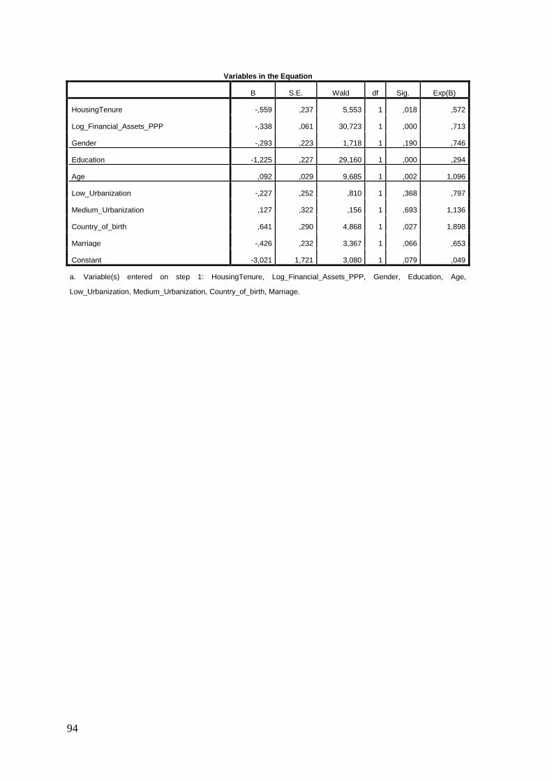
94
Variables in the Equation
B S.E. Wald df Sig. Exp(B)
HousingTenure -,559 ,237 5,553 1 ,018 ,572
Log_Financial_Assets_PPP -,338 ,061 30,723 1 ,000 ,713
Gender -,293 ,223 1,718 1 ,190 ,746
Education -1,225 ,227 29,160 1 ,000 ,294
Age ,092 ,029 9,685 1 ,002 1,096
Low_Urbanization -,227 ,252 ,810 1 ,368 ,797
Medium_Urbanization ,127 ,322 ,156 1 ,693 1,136
Country_of_birth ,641 ,290 4,868 1 ,027 1,898
Marriage -,426 ,232 3,367 1 ,066 ,653
Constant -3,021 1,721 3,080 1 ,079 ,049
a. Variable(s) entered on step 1: HousingTenure, Log_Financial_Assets_PPP, Gender, Education, Age,
Low_Urbanization, Medium_Urbanization, Country_of_birth, Marriage.
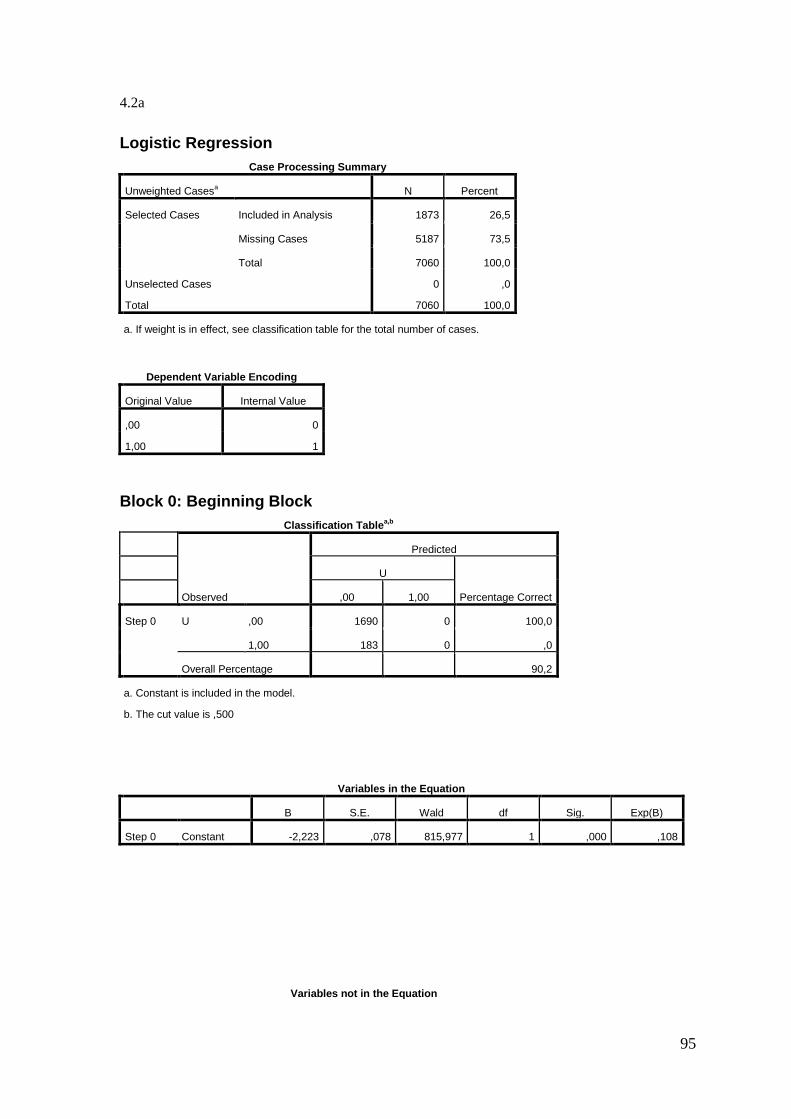
95
4.2a
Logistic Regression
Case Processing Summary
Unweighted Casesa N Percent
Selected Cases Included in Analysis 1873 26,5
Missing Cases 5187 73,5
Total 7060 100,0
Unselected Cases 0 ,0
Total 7060 100,0
a. If weight is in effect, see classification table for the total number of cases.
Dependent Variable Encoding
Original Value Internal Value
,00 0
1,00 1
Block 0: Beginning Block
Classification Tablea,b
Observed
Predicted
U
Percentage Correct
,00 1,00
Step 0 U ,00 1690 0 100,0
1,00 183 0 ,0
Overall Percentage 90,2
a. Constant is included in the model.
b. The cut value is ,500
Variables in the Equation
B S.E. Wald df Sig. Exp(B)
Step 0 Constant -2,223 ,078 815,977 1 ,000 ,108
Variables not in the Equation

96
Score df Sig.
Step 0 Variables HousingTenure_t_1 13,296 1 ,000
Gender ,305 1 ,581
Age 1,807 1 ,179
Overall Statistics 15,695 3 ,001
Block 1: Method = Enter
Omnibus Tests of Model Coefficients
Chi-square df Sig.
Step 1 Step 14,773 3 ,002
Block 14,773 3 ,002
Model 14,773 3 ,002
Model Summary
Step -2 Log likelihood
Cox & Snell R
Square
Nagelkerke R
Square
1 1183,981a ,008 ,017
a. Estimation terminated at iteration number 5 because parameter
estimates changed by less than ,001.
Classification Tablea
Observed
Predicted
U
Percentage Correct
,00 1,00
Step 1 U ,00 1690 0 100,0
1,00 183 0 ,0
Overall Percentage 90,2
a. The cut value is ,500

97
Variables in the Equation
B S.E. Wald df Sig. Exp(B)
Step 1a HousingTenure_t_1 -,608 ,166 13,418 1 ,000 ,545
Gender -,127 ,158 ,649 1 ,420 ,881
Age ,035 ,028 1,629 1 ,202 1,036
Constant -3,805 1,642 5,370 1 ,020 ,022
a. Variable(s) entered on step 1: HousingTenure_t_1, Gender, Age.
Correlation Matrix
Constant HousingTenure_t_1 Gender Age
Step 1 Constant 1,000 -,078 -,113 -,995
HousingTenure_t_1 -,078 1,000 ,105 ,007
Gender -,113 ,105 1,000 ,060
Age -,995 ,007 ,060 1,000
4.3a
Logistic Regression
Case Processing Summary
Unweighted Casesa N Percent
Selected Cases Included in Analysis 1297 18,4
Missing Cases 5763 81,6
Total 7060 100,0
Unselected Cases 0 ,0
Total 7060 100,0
a. If weight is in effect, see classification table for the total number of cases.
Dependent Variable Encoding
Original Value Internal Value
,00 0
1,00 1

98
Classification Tablea,b
Observed
Predicted
U
Percentage Correct
,00 1,00
Step 0 U ,00 1187 0 100,0
1,00 110 0 ,0
Overall Percentage 91,5
a. Constant is included in the model.
b. The cut value is ,500
Variables in the Equation
B S.E. Wald df Sig. Exp(B)
Step 0 Constant -2,379 ,100 569,619 1 ,000 ,093
Omnibus Tests of Model Coefficients
Chi-square df Sig.
Step 1 Step 163,251 16 ,000
Block 163,251 16 ,000
Model 163,251 16 ,000
Model Summary
Step -2 Log likelihood Cox & Snell R Square Nagelkerke R Square
1 589,957a ,118 ,268
a. Estimation terminated at iteration number 7 because parameter estimates
changed by less than ,001.
Classification Tablea
Observed
Predicted
U
Percentage Correct
,00 1,00
Step 1 U ,00 1174 13 98,9
1,00 98 12 10,9
Overall Percentage 91,4
a. The cut value is ,500

99
Variables in the Equation
B S.E. Wald df Sig. Exp(B)
HousingTenure -,680 ,257 6,982 1 ,008 ,506
Log_Financial_Assets_PPP -,319 ,065 23,804 1 ,000 ,727
Gender -,260 ,232 1,251 1 ,263 ,771
Education -,891 ,258 11,929 1 ,001 ,410
Age ,070 ,031 5,140 1 ,023 1,072
Low_Urbanization -,141 ,263 ,289 1 ,591 ,868
Medium_Urbanization ,306 ,348 ,774 1 ,379 1,358
Country_of_birth ,496 ,308 2,589 1 ,108 1,642
Marriage -,367 ,244 2,260 1 ,133 ,693
Austria -,687 ,346 3,958 1 ,047 ,503
Spain ,199 ,384 ,268 1 ,605 1,220
Italy -1,423 ,604 5,541 1 ,019 ,241
France -1,082 ,601 3,244 1 ,072 ,339
Denmark -1,855 ,789 5,531 1 ,019 ,156
Switzerland -1,181 ,423 7,813 1 ,005 ,307
CzechRepublic -1,479 ,451 10,784 1 ,001 ,228
Constant -1,419 1,867 ,578 1 ,447 ,242
a. Variable(s) entered on step 1: HousingTenure, Log_Financial_Assets_PPP, Gender, Education, Age,
Low_Urbanization, Medium_Urbanization, Country_of_birth, Marriage, Austria, Spain, Italy, France, Denmark,
Switzerland, CzechRepublic.

100
4.4a
Logistic Regression
Case Processing Summary
Unweighted Casesa N Percent
Selected Cases Included in Analysis 992 14,1
Missing Cases 6068 85,9
Total 7060 100,0
Unselected Cases 0 ,0
Total 7060 100,0
a. If weight is in effect, see classification table for the total number of cases.
Dependent Variable Encoding
Original Value Internal Value
,00 0
1,00 1
Block 0: Beginning Block
Classification Tablea,b
Observed
Predicted
U
Percentage Correct
,00 1,00
Step 0 U ,00 933 0 100,0
1,00 59 0 ,0
Overall Percentage 94,1
a. Constant is included in the model.
b. The cut value is ,500
Variables in the Equation
B S.E. Wald df Sig. Exp(B)
Step 0 Constant -2,761 ,134 422,974 1 ,000 ,063
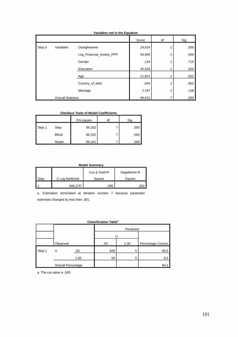
101
Variables not in the Equation
Score df Sig.
Step 0 Variables Outrightowner 24,024 1 ,000
Log_Financial_Assets_PPP 55,900 1 ,000
Gender ,134 1 ,715
Education 45,628 1 ,000
Age 11,821 1 ,001
Country_of_birth ,004 1 ,952
Marriage 2,197 1 ,138
Overall Statistics 99,012 7 ,000
Omnibus Tests of Model Coefficients
Chi-square df Sig.
Step 1 Step 99,162 7 ,000
Block 99,162 7 ,000
Model 99,162 7 ,000
Model Summary
Step -2 Log likelihood
Cox & Snell R
Square
Nagelkerke R
Square
1 348,275a ,095 ,262
a. Estimation terminated at iteration number 7 because parameter
estimates changed by less than ,001.
Classification Tablea
Observed
Predicted
U
Percentage Correct
,00 1,00
Step 1 U ,00 928 5 99,5
1,00 54 5 8,5
Overall Percentage 94,1
a. The cut value is ,500

102
Variables in the Equation
B S.E. Wald df Sig. Exp(B)
Outrightowner ,756 ,346 4,769 1 ,029 2,129
Log_Financial_Assets_PPP -,471 ,086 29,763 1 ,000 ,625
Gender -,217 ,303 ,513 1 ,474 ,805
Education -1,304 ,312 17,412 1 ,000 ,272
Age ,135 ,042 10,527 1 ,001 1,145
Country_of_birth ,228 ,549 ,173 1 ,677 1,257
Marriage -,128 ,339 ,143 1 ,705 ,880
Constant -5,767 2,382 5,861 1 ,015 ,003
a. Variable(s) entered on step 1: Outrightowner, Log_Financial_Assets_PPP, Gender, Education, Age, Country_of_birth,
Marriage.
4.5a
Logistic Regression
Case Processing Summary
Unweighted Casesa N Percent
Selected Cases Included in Analysis 1437 20,4
Missing Cases 5623 79,6
Total 7060 100,0
Unselected Cases 0 ,0
Total 7060 100,0
a. If weight is in effect, see classification table for the total number of cases.
Dependent Variable Encoding
Original Value Internal Value
,00 0
1,00 1

103
Classification Tablea,b
Observed
Predicted
U
Percentage Correct
,00 1,00
Step 0 U ,00 1317 0 100,0
1,00 120 0 ,0
Overall Percentage 91,6
a. Constant is included in the model.
b. The cut value is ,500
Variables in the Equation
B S.E. Wald df Sig. Exp(B)
Step 0 Constant -2,396 ,095 631,170 1 ,000 ,091
Variables not in the Equation
Score df Sig.
Step 0 Variables OutrightOwner_t_1 20,369 1 ,000
Gender ,097 1 ,756
Age ,000 1 ,986
Overall Statistics 20,455 3 ,000
Block 1: Method = Enter
Omnibus Tests of Model Coefficients
Chi-square df Sig.
Step 1 Step 20,101 3 ,000
Block 20,101 3 ,000
Model 20,101 3 ,000

104
Model Summary
Step -2 Log likelihood
Cox & Snell R
Square
Nagelkerke R
Square
1 805,464a ,014 ,032
a. Estimation terminated at iteration number 6 because parameter
estimates changed by less than ,001.
Classification Tablea
Observed
Predicted
U
Percentage Correct
,00 1,00
Step 1 U ,00 1317 0 100,0
1,00 120 0 ,0
Overall Percentage 91,6
a. The cut value is ,500
Variables in the Equation
B S.E. Wald df Sig. Exp(B)
Step 1a OutrightOwner_t_1 ,862 ,196 19,423 1 ,000 2,367
Gender ,045 ,193 ,054 1 ,815 1,046
Age ,007 ,035 ,041 1 ,840 1,007
Constant -3,261 2,050 2,529 1 ,112 ,038
a. Variable(s) entered on step 1: OutrightOwner_t_1, Gender, Age.
Correlation Matrix
Constant OutrightOwner_t_1 Gender Age
Step 1 Constant 1,000 -,100 -,131 -,996
OutrightOwner_t_1 -,100 1,000 -,016 ,044
Gender -,131 -,016 1,000 ,087
Age -,996 ,044 ,087 1,000

105
4.1b
Logistic Regression
Case Processing Summary
Unweighted Casesa N Percent
Selected Cases Included in Analysis 115 1,6
Missing Cases 6945 98,4
Total 7060 100,0
Unselected Cases 0 ,0
Total 7060 100,0
a. If weight is in effect, see classification table for the total number of cases.
Dependent Variable Encoding
Original Value Internal Value
,00 0
1,00 1
Block 0: Beginning Block
Classification Tablea,b
Observed
Predicted
ULT
Percentage Correct
,00 1,00
Step 0 ULT ,00 0 52 ,0
1,00 0 63 100,0
Overall Percentage 54,8
a. Constant is included in the model.
b. The cut value is ,500
Variables in the Equation
B S.E. Wald df Sig. Exp(B)
Step 0 Constant ,192 ,187 1,049 1 ,306 1,212
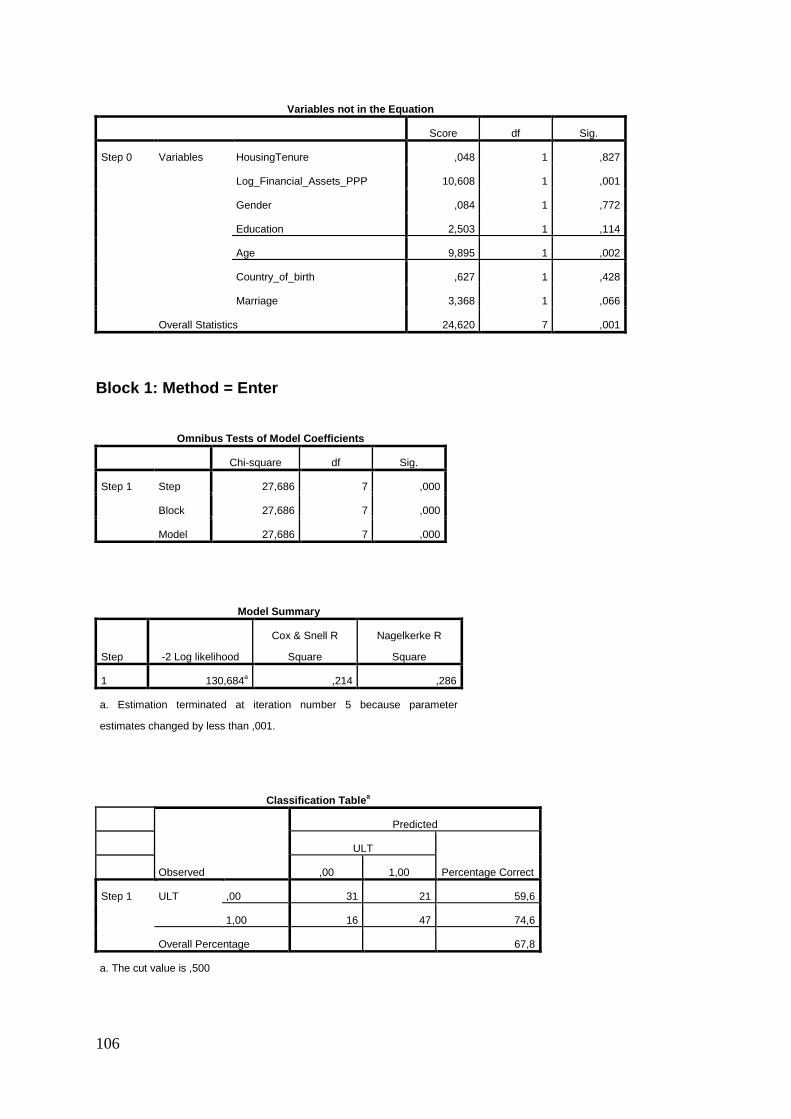
106
Variables not in the Equation
Score df Sig.
Step 0 Variables HousingTenure ,048 1 ,827
Log_Financial_Assets_PPP 10,608 1 ,001
Gender ,084 1 ,772
Education 2,503 1 ,114
Age 9,895 1 ,002
Country_of_birth ,627 1 ,428
Marriage 3,368 1 ,066
Overall Statistics 24,620 7 ,001
Block 1: Method = Enter
Omnibus Tests of Model Coefficients
Chi-square df Sig.
Step 1 Step 27,686 7 ,000
Block 27,686 7 ,000
Model 27,686 7 ,000
Model Summary
Step -2 Log likelihood
Cox & Snell R
Square
Nagelkerke R
Square
1 130,684a ,214 ,286
a. Estimation terminated at iteration number 5 because parameter
estimates changed by less than ,001.
Classification Tablea
Observed
Predicted
ULT
Percentage Correct
,00 1,00
Step 1 ULT ,00 31 21 59,6
1,00 16 47 74,6
Overall Percentage 67,8
a. The cut value is ,500

107
Variables in the Equation
B S.E. Wald df Sig. Exp(B)
HousingTenure -,665 ,499 1,772 1 ,183 ,514
Log_Financial_Assets_PPP -,484 ,149 10,496 1 ,001 ,617
Gender ,065 ,462 ,020 1 ,888 1,067
Education -,393 ,460 ,731 1 ,393 ,675
Age ,190 ,064 8,931 1 ,003 1,209
Country_of_birth -,843 ,612 1,898 1 ,168 ,430
Marriage ,782 ,454 2,964 1 ,085 2,185
Constant -6,335 3,546 3,191 1 ,074 ,002
4.2b
Logistic Regression
Case Processing Summary
Unweighted Casesa N Percent
Selected Cases Included in Analysis 157 2,2
Missing Cases 6903 97,8
Total 7060 100,0
Unselected Cases 0 ,0
Total 7060 100,0
a. If weight is in effect, see classification table for the total number of cases.
Dependent Variable Encoding
Original Value Internal Value
,00 0
1,00 1
Block 0: Beginning Block
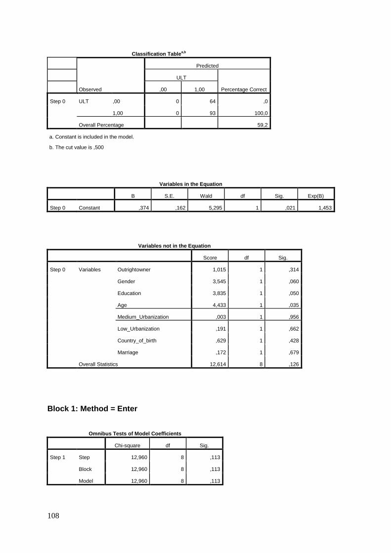
108
Classification Tablea,b
Observed
Predicted
ULT
Percentage Correct
,00 1,00
Step 0 ULT ,00 0 64 ,0
1,00 0 93 100,0
Overall Percentage 59,2
a. Constant is included in the model.
b. The cut value is ,500
Variables in the Equation
B S.E. Wald df Sig. Exp(B)
Step 0 Constant ,374 ,162 5,295 1 ,021 1,453
Variables not in the Equation
Score df Sig.
Step 0 Variables Outrightowner 1,015 1 ,314
Gender 3,545 1 ,060
Education 3,835 1 ,050
Age 4,433 1 ,035
Medium_Urbanization ,003 1 ,956
Low_Urbanization ,191 1 ,662
Country_of_birth ,629 1 ,428
Marriage ,172 1 ,679
Overall Statistics 12,614 8 ,126
Block 1: Method = Enter
Omnibus Tests of Model Coefficients
Chi-square df Sig.
Step 1 Step 12,960 8 ,113
Block 12,960 8 ,113
Model 12,960 8 ,113
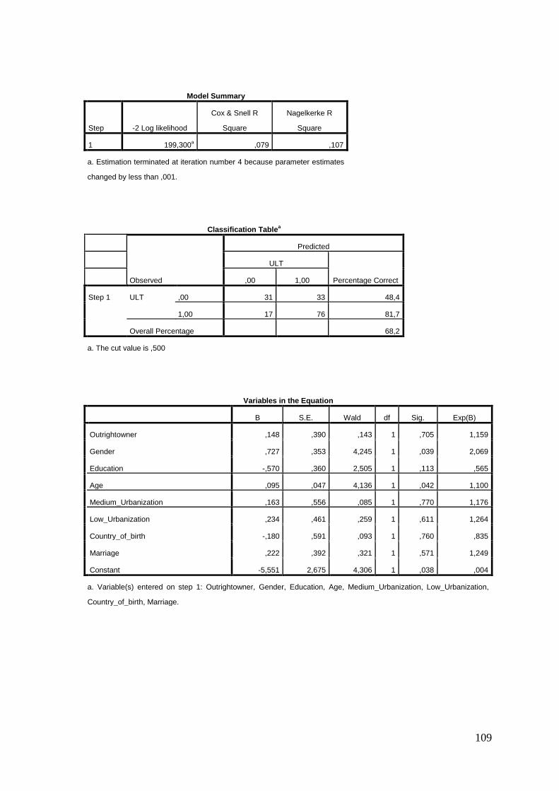
109
Model Summary
Step -2 Log likelihood
Cox & Snell R
Square
Nagelkerke R
Square
1 199,300a ,079 ,107
a. Estimation terminated at iteration number 4 because parameter estimates
changed by less than ,001.
Classification Tablea
Observed
Predicted
ULT
Percentage Correct
,00 1,00
Step 1 ULT ,00 31 33 48,4
1,00 17 76 81,7
Overall Percentage 68,2
a. The cut value is ,500
Variables in the Equation
B S.E. Wald df Sig. Exp(B)
Outrightowner ,148 ,390 ,143 1 ,705 1,159
Gender ,727 ,353 4,245 1 ,039 2,069
Education -,570 ,360 2,505 1 ,113 ,565
Age ,095 ,047 4,136 1 ,042 1,100
Medium_Urbanization ,163 ,556 ,085 1 ,770 1,176
Low_Urbanization ,234 ,461 ,259 1 ,611 1,264
Country_of_birth -,180 ,591 ,093 1 ,760 ,835
Marriage ,222 ,392 ,321 1 ,571 1,249
Constant -5,551 2,675 4,306 1 ,038 ,004
a. Variable(s) entered on step 1: Outrightowner, Gender, Education, Age, Medium_Urbanization, Low_Urbanization,
Country_of_birth, Marriage.