0

Faculty of Bioscience Engineering

Academic year 2015 – 2016

Ecological assessment of Portoviejo river basin (Ecuador)

Juan Antonio Dueñas Utreras

Promotor: Prof. dr. ir. Peter L.M. Goethals

Tutor: MSc. Marie Anne Eurie Forio

Master’s dissertation submitted in partial fulfillment of the requirements

for the degree of

Master of Science in Environmental Sanitation

0

i

COPYRIGHT PAGE

I, JUAN ANTONIO DUEÑAS UTRERAS, herewith declare that this dissertation is the result of my

own work and the submission of this dissertation is only made here in this university. Other

studies used here have been duly acknowledged through references of the authors and served

as information resources.

The author and the promoter give authorization to consult and copy parts of this dissertation for

personal use only. Any other use of this dissertation is subject to copyrights laws, and the source

should be specified after having received the written permission from the author and the

promoter.

Laboratory for Environmental Toxicology and Aquatic Ecology

Department of Applied Ecology and Environmental Biology

Faculty of Bio-engineering Sciences, Ghent University

Jozef Plateaustraat 22, B-9000 Gent (Belgium)

Tel. 0032 (0)9643765 Fax. 0032 (0) 9 2644199

…………………………………………

19/08/2016

Prof. Dr. ir. Peter L.M. Goethals

(Promoter)

Email: peter.goethals@UGent.be

……………………………………………

19/08/2016

Juan Antonio Dueñas Utreras

(Master thesis author)

Email: jadu333@hotmail.com

ii

ACKNOWLEDGMENTS

First at all, I want to thanks God who has given to me the strength to remain firm in my convictions

and who holding me in my moments of sadness.

To my Promotor Prof. Peter Goethals and my tutor Marie Anne Eurie Forio, who have contributed

to my training, thanks for all your help in the realization of this thesis.

Special thanks to the Ministry of Higher Education, Science and Technology and Innovation

(SENESCYT) of Ecuador for the scholarship that was awarded in 2014 that made me able to realize

my dreams of studying abroad.

The Technical University of Manabí, institution where I work, thank you very much for the trust.

To my beloved Erika for giving me unconditional love and constant support at all times, my little

Lina for giving me their love and happiness when I needed it.

My mother, who provide their prayers and affection throughout my life, to each of the members

of my family, my grandfather, uncles, sisters, nephews, nieces and cousins.

To my friends in Ghent, who tolerated my jokes, for his words of encouragement and especially

for his sincere friendship in these two years where they became my family in foreign land.

To Anne-Marie and Guy for accepting me into your home and make me feel at home.

My eternal gratitude.

iii

TABLE OF CONTENT

COPYRIGHT PAGE .............................................................................................................................. i

ACKNOWLEDGMENTS ...................................................................................................................... ii

TABLE OF CONTENT ......................................................................................................................... iii

LIST OF ABBREVIATIONS ................................................................................................................... v

ABSTRACT ....................................................................................................................................... vii

1. INTRODUCTION ............................................................................................................................ 1

2. LITERATURE REVIEW ..................................................................................................................... 3 2.1 Water Quality in freshwater ecosystems .............................................................................. 3

2.2 Quality indices ....................................................................................................................... 3

2.2.1 Biological Indices ............................................................................................................ 3

2.2.2 Physicochemical water quality ....................................................................................... 6

2.3 River Continuum Concept (RCC) ............................................................................................ 8

2.4 Impacts of pollution............................................................................................................. 11

3. MATERIALS AND METHODS ............................................................................................... 13

3.1. Study area ........................................................................................................................... 13

3.2 Data collection ..................................................................................................................... 14

3.2.1 Macroinvertebrates ...................................................................................................... 14

3.2.2. Physicochemical characteristics .................................................................................. 14

3.2.3. Hydromorphological characteristics ............................................................................ 15

3.3. Chemical and ecological assessment .................................................................................. 15

3.3.1. Chemical indices .......................................................................................................... 15

3.3.2. Ecological indices ......................................................................................................... 16

3.4. Scatter plots and boxplots .................................................................................................. 17

3.5. Data analysis ....................................................................................................................... 18

4. RESULTS ...................................................................................................................................... 19 4.1 Physicochemical results ....................................................................................................... 19

4.2. Macroinvertebrates ............................................................................................................ 20

iv

4.3 Water Quality Indices .......................................................................................................... 23

4.4. Gradients of environmental variables from mouth to source. .......................................... 25

4.5. Impacts of dams ................................................................................................................. 29

4.6. Impact of Land use ............................................................................................................. 31

4.7 Effect of municipal waste water treatment plants ............................................................. 34

5. DISCUSSION ................................................................................................................................ 36 5.1 Water quality ....................................................................................................................... 36

5.2 River continuum/ Gradients from source to mouth ........................................................... 37

5.3 Impacts ................................................................................................................................ 39

5.3.1 Impact causes by dams in Portoviejo river ................................................................... 39

5.3.2 Impact of Portoviejo river cause by land use ............................................................... 40

5.3.3 Effects of municipal wastewater treatment plant in the Portoviejo river basin .......... 41

6. CONCLUSIONS AND RECOMMENDATIONS ................................................................................ 43 6.1 Conclusions .......................................................................................................................... 43

6.2 Recommendations. .............................................................................................................. 44

REFERENCES ................................................................................................................................... 45

APPENDICES .................................................................................................................................... 54

v

LIST OF ABBREVIATIONS

BMWP: Biological Monitoring Working Party

BOD: Biological Oxygen Demand

BOD5: Five days Biological Oxygen Demand

COD: Chemical Oxygen Demand

CPOM: Coarse Particulate Organic Matter

DO: Dissolved Oxygen

DOM: Dissolved Organic matter

DOsat: Dissolved Oxygen Saturation

EC: Electrical Conductivity

EIFA-WP: European Inland Fishery Advisory

commission Working Party

EPT: Ephemeroptera, Plecoptera and Trichoptera

FFG: Functional Feeding Groups

FISRWG: Federal Interagency Stream Restoration

Working Group

INAMHI: Instituto Nacional de Meteorología e

Hidrología

INEC: Instituto Nacional de Estadística y Censos

MAGAP: Ministerio de Agricultura, Ganadería,

Acuacultura y Pesca.

MMIF: Multimetric Macroinvertebrate Index for

Flanders

PCBs: Poly-Chlorobiphenols

PHCs: Poly Aromatic Hydrocarbons

RCC: River Continuum Concept

SENAGUA: Secretaria Nacional del Agua

TOC: Total Organic Carbon

vi

WATQI: Water Quality Index

CF : Coliform fecal

ATP : Adenosine triphosphate

vii

ABSTRACT

Water is essential for life of organisms and necessary in civilization. However, the fast growth of

the human population, changes in land use and rapid urbanization damage natural ecosystems

and reduce their value for delivering goods and services for human societies. Around the world,

various researches determine how ecosystems respond to external stressors. However, some

regions are hardly investigated and characterized. For instance, the water and ecological quality

of the Portoviejo river basin is unknown.

Thus, the present study assesses the water quality of the Portoviejo River in Ecuador.

Furthermore, the evolution of various environmental variables was determined along the

disturbance gradient within the river. Additionally, the impacts of irrigation dams, agriculture,

urbanization, wastewater discharge on water and ecological quality was assessed. For this,

physical, chemical and biological (macroinvertebrates) characteristics of the rivers were sampled

at 31 sampling sites along the main river, some tributaries and within the reservoir. Ecological

quality, expressed as Biological Monitoring Working Party-Colombia (BMWP-Col), and chemical

indices (the Dutch and LISEC methods) were calculated. Majority of sampling sites (45%) had poor

quality. The good ecological quality was associated with high flow velocities, low temperatures,

low conductivity, low chlorophyll a content, low biological oxygen demand (BOD5) and low

nutrient concentrations. Additionally, good water quality was also associated with the presence

of sensitive taxa and high diversity. Bad quality, mainly at the downstream of the river, is related

to urbanization and inputs of untreated domestic wastewater. In general, there was an increase

in conductivity, chlorophyll a, available nutrients, and total organic carbon along the gradient

from source to the mouth. This observation was related to changes in land use. Predators and

collectors were dominant at upstream, more scrapers were found at the midstream and collectors

dominated near to the mouth. Deviation from the prediction of the River Continuum Concept

(RCC) can be explained by the presence of a series of dams along the river and differences in food

availability in tropical zones. Flow velocity, pH and temperature are low before dams. While,

turbidity is relatively high after dams. Chlorophyll a is higher in residential areas than in forest and

arable land. While conductivity and nutrients in forest areas are relatively low compared with

arable land. Conversely, BOD5 in forest areas is relatively higher than in arable and residential

zones. Physicochemical variables are not statistically affected by the presence of a municipal

WWTP in the Portoviejo River. Nonetheless, chlorophyll a, BOD5, TOC, total phosphorus and total

nitrogen after WWTP are relatively higher than before WWTP. Probably, the WWTP is insufficient

in organic and nutrients removal or an overload of waste is present.

In general, Portoviejo River follows the pollution gradient typical by the presence of

anthropogenic perturbations. Based on the findings, a sustainable management of the river

catchment is necessary, combining the reduction of inflow of pollutants via wastewater

treatment, and minimizing the habitat alteration of banks, and restoring flows affected by

hydropower dams.

1

1. INTRODUCTION

Water is essential for life of organisms. It is necessary for development of natural ecosystems, for

human well-being and for progress of cities (Virha et al., 2011; Haldar et al., 2014). Around the

world, freshwater is mainly obtained from natural streams which are exposed to external pressure

that could influence its water quality. Water quality, in most cases, is caused by human activities

such as water pollution, modification of natural hydrology, river impoundments and land-use

changes (Geist, 2011). Assessment of water quality is crucial to determine the health of

ecosystems, control of environmental pollution and hence to maintain human safety (Bilotta et

al., 2008). Nowadays, water quality is assessed by measuring environmental variables and by

freshwater organisms in order to determine the environmental status of the ecosystem

(Sundermann et al., 2015). The use of macroinvertebrates together with physicochemical

variables has been used worldwide to assess water quality. Some adaptations were made to allow

its use in all regions including South America (Damanik-Ambarita et al., 2016). Macroinvertebrates

are broadly used because it provides an easy and less costly tool to monitor freshwater

ecosystems, which make it the best option in developing countries (Pander and Geist, 2013).

In Ecuador, a number of investigations on water quality and ecological status on freshwater

ecosystems based on macroinvertebrates were implemented (Alvarez-Mieles et al., 2013,

Damanik-Ambarita et al., 2016). However, this method is not yet spread along the whole country,

such as the case of the Portoviejo River. The Portoviejo River is an important source of water for

the inhabitants of the region for drinking water and irrigation. To know its water quality status is

crucial in order to take actions for reducing sources and impacts of pollution. However, the water

and ecological quality of the Portoviejo river basin is unknown. It is currently monitored based on

physicochemical variables by the water secretariat (Secretaría del agua SENAGUA), a government

organization which is also in charge to assure the access to good quality freshwater for human

consumption, irrigation and other uses. Furthermore, the conservation of natural environment is

in charge of the ministry of environment (Ministerio del ambiente MAE), which is in charge to

ensure sustainable management of strategic natural resources. Together, both agencies are

making good effort to assure water supply in the region but the rapid population grow,

urbanization, changes in land use, together with limited budget make it challenging to control and

continuously monitor the freshwater streams. Furthermore, the municipal government is putting

a great effort to recover the water quality of the river but positive results are not yet obtained.

Portoviejo river consists of a series of dams. The impacts of irrigation dams in water and ecological

quality are unknown. Furthermore, little is known on the impact of a series of dams along a

tropical river on the functional feeding groups (FFG). In the same way, limited knowledge exists

in how the nutrients, organic matter and others physicochemical variables evolve in this system.

The Portoviejo offers an interesting advantage for study as it is a small catchment (system) and

thus it is easy to explore and be investigated. As various land uses such as agriculture, and

urbanization and the presence of dams are found along the Portoviejo river impacts of these land

uses can be easily studied. Thus, changes in land use and other anthropogenic activities could be

2

anticipated in order to reduce pollution to the river. Findings of this study can be used as a

baseline on the effects of these anthropogenic activities in a similar tropical river system

worldwide.

For reasons cited above, an ecological monitoring based on macroinvertebrates is proposed to

identify multiple stressors in freshwater stream to help decision makers to take actions for

management and control pollution.

For this research, it is aimed (1) to assess the ecological water quality in the Portoviejo River

(Ecuador) based on macroinvertebrates community, (2) to analyze the environmental gradients

along the river based on the river continuum concept and (3) to estimate different impacts caused

by land use, dams and waste water treatment plants within the Portoviejo River.

3

2. LITERATURE REVIEW

2.1 Water Quality in freshwater ecosystems

Water is essential for the life in the planet (Virha et al., 2011). Freshwater streams support the

natural ecosystem (Haldar et al., 2014). People use freshwater mainly from rivers for their daily

activities. Utilization of water resources is indispensable for humans and its use has allowed the

development of cities and countries (Geist, 2011; Kaushal et al., 2015; Pander et al., 2013).

Water quality is important for sustaining development of both human and ecological communities

(Srebotnjak et al., 2012). Water quality could be defined as a group of chemical and physical

characteristics of any stream that could be used as indicator of ecosystem health and useful for

deducting environmental pollution (Bilotta et al, 2008). To assess water quality, environmental

measurements are needed. These values are usually contrasted with a reference point that has

previously been considered as good water quality site (De Rosemond et al., 2009).

The sources of pollutants are different and are present in many forms. Diffuse and point source

pollution affects streams in distinct ways. They may degrade various aquatic habitats through

accumulation. For instance, major intensity usually occurs in the lower section of a stream,

impoverishing the water quality and results to a decrease in diversity of aquatic fauna (Snook and

Whitehead, 2004). Furthermore, other types of river alteration, such as modification of natural

hydrology of a stream, also leads to the detriment of water quality (Castello and Macedo, 2016).

European Inland Fishery Advisory commission Working Party (EIFA-WP) defined parameters for

water quality in 1969. They demarcated safe pH range for fish, which is between 5 and 9.

Furthermore, they also established healthy temperature and ammonia ranges for aquatic animals

(EIFA-WP, 1969). In various studies, freshwater quality is derived from physicochemical, biological

and microbiological parameters (Antonietti et al., 1996; Da Silva and Sacomani, 2001; Reisenhofer

et al., 1998). These include pH, COD, orthophosphates, conductivity, dissolved oxygen, total

plating count, ammonia, nitrate, alkalinity, coliform fecal CF, adenosine triphosphate ATP,

carbohydrates and macrobenthos composition (Antonietti et al., 1996). In 2008, a Water Quality

Index (WATQI) was developed based on five parameters: dissolved oxygen, electrical conductivity,

total phosphorous, total nitrogen and pH (Srebotnjak et al., 2012).

2.2 Quality indices

2.2.1 Biological Indices

Several studies revealed that biota depends on water quality. Mostly, water quality is influenced

by anthropogenic pressures such as urbanization and agriculture (Kail et al., 2012). Organisms in

freshwater bodies seem to suffer multiple stressors from human activities and therefore these

organisms serve as indicators for pollution (Sundermann et al., 2015). Globally, freshwater

organisms are used to assess water quality and determine the environmental status of an

ecosystem.

4

Fish, invertebrates, algae and macrophytes are commonly used to assess quality of aquatic

environments. They provide an easy and less costly tool to monitor the ecological status of

freshwater ecosystems (Southerland et al., 2007; Pander et al., 2013). But some of them have

limitations. For instance, fish monitoring cannot be applied to very small streams due to the

impairment of space to their developing (Southerland et al., 2007). Additionally, stream quality

classifications are usually based on the presence of expected fauna from a reference site (pristine

location). In this way, the absence of fauna means presence of stressors. Nevertheless, it needs

to take into account that these variations could depend on other physical characteristics, such as

landscape and flow velocity (Skoulikidis et al., 2009).

Macroinvertebrates are broadly used in environmental assessment as they are sensitive for a wide

range of pollutants. They have a broad variety of taxonomic groups whose responses towards

environmental variations are very valuable to evaluate freshwater ecosystems (Carlisle et al.,

2007; Smith et al., 2007). Cao et al., (1997) found as water quality was reduced along the stream,

some species loses their average quantity. On the other hand, the number of some tolerant

species increased in the contaminated sites. Furthermore, they measure the cumulative response

to habitat changes due to their long life cycle (Azevedo et al., 2015).

Macroinvertebrates has been used as water quality indicators since early 1950s (Gabriels, 2007)

and several assessment methods has been developed worldwide to evaluate water quality

(Skoulikidis et al., 2009). As an example a Multimetric Macroinvertebrates Index for Flanders

(MMIF) was developed by Gabriels et al. (2010) to assess quality in rivers and lakes within Belgium.

In Bulgaria and Vietnam, freshwater quality was determined with macroinvertebrates (Lock et al.,

2011; Nguyen et al., 2014). Furthermore, hydromorphological quality on surface water was also

examined in Estonia based on invertebrates (Timm et al., 2011).

2.2.1.1 Common indices based on Macroinvertebrates

There is an ample quantity of indices based on macroinvertebrates communities to assess

freshwater quality (Gabriels, 2007). Some of them used in the present study are discussed in the

following paragraphs.

Biological Monitoring Working Party (BMWP)

The Biological Monitoring Working Party (BMWP) (Armitage et al., 1983) developed in UK and

revised by the National Water Council, is based in a score system (Couto-Mendoza et al., 2015).

The BMWP score provides a suitable classification for monitoring and assessing quality in

freshwater ecosystem (Armitage et al., 1983). Zamora-Muñoz et al. (1995) demonstrated that

BMWP is negatively related to pollution. Their study also indicates that BMWP is not seasonally

dependent (Zamora-Muñoz et al., 1995) making it suitable for monitoring campaign during all

seasons.

Some adaptations to BMWP index were made in Europe. For example, the Iberian Biological

Monitoring Working Party (IBMWP) for Spain (Alba-Tercedor 2000; Alba-Tercedor et al., 2004)

5

was developed. According to Couto-Mendoza et al. (2015), IBMWP was more used during the last

two and a half decades in Spain to determine ecological status in freshwater.

Several adaptations from BMWP have been developed in Latin America. For instance, in Costa

Rica, the Biological Monitoring Working Party Costa Rica (BMWP-CR) is employed (Gutiérrez and

Lorion, 2014). In Colombia, Roldán (2003) established Biological Monitoring Working Party

Colombia (BMWP/Col) to make an approximation on the ecological status of water bodies in

Colombia (Roldán, 2003). Some researches were conducted applying BMWP-Col in Colombia

(Montoya et al., 2011; Forero and Reinoso, 2013) and in Ecuador (Alvarez-Mieles et al., 2013;

Damanik-Ambarita et al., 2016) to assess freshwater quality and wetland ecosystems.

Diversity indices

Shannon-Wiener (Shannon and Weaver, 1949) and Margalef index (Margalef, 1958) are non-

taxonomic metrics (Gabriels, 2007), also referred as diversity indices. Both metrics make use of

richness, evenness and abundance on macroinvertebrate community. In an unpolluted

environment, high richness, even-spreading and abundant organisms is expected (Metcalfe,

1989). Metcalfe (1989) describes some advantages of diversity indices. They are exclusively

quantitative, independent of the proportions of the sample, no suppositions about tolerances are

needed and can measure biomass instead count individuals. Criticism against it includes values

rely on the equation used, there are variations depending on the standard used, some species are

neglected, it considers response to pollution as linear, and there is few testing in middle range

pollution (Metcalfe, 1989).

Taxonomic species richness

Freshwater invertebrate richness in pristine locations is influenced by environmental factors such

as geology, ecosystem productivity, competition and predation. Interactions of these factors

determine the gradients of species richness (Compin and Céréghino, 2003). The richness along

the stream is influenced by anthropogenic interference (Céréghino et al. 2003). The number of

taxa reduced (Brittain and Saltveit as cited by Compin and Céréghino, 2003) and expected gradient

is disrupted (Ward and Stanford as cited by Compin and Céréghino, 2003) as a result of human

activities.

Because Ephemeroptera, Plecoptera and Trichoptera (EPT) have an extensive distribution, they

are highly associated with tendencies in richness and vastly related with ecological variations

(Shah et al. 2015). Thus, EPT is a good indicator of stream disturbances (Céréghino et al. 2003).

EPT taxa were used to assess stream ecosystem health in Burkina Faso in Africa (Kaboré et al.

2016) and in Latin America and the Caribbean (Soldner et al. 2014).

The number of macroinvertebrate families are also used as an indicator of pollution in freshwater

streams (Carlisle et al. 2007). Carlisle et al. (2007) found that genera and families are strongly

correlated to road density as a result of urbanization. The total number of taxa is also utilized to

derive the multimetric index in Belgium (Gabriels, 2010) and in Vietnam (Nguyen et al. 2014).

6

2.2.2 Physicochemical water quality

Physical and chemical properties depict water of a stream (Bilotta et al. 2008) and are essential

determining the stream’s quality (Virha et al. 2011). As the population grows, the needs of

freshwater increase as well. Furthermore, as a result of the increase of anthropogenic activities,

biological and physicochemical conditions of rivers deteriorate (Forero-Céspedes and Reinoso-

Flórez, 2013).

Pollution caused by chemicals is the main stressor in freshwater ecosystems (Berger el al. 2016).

Berger el al. (2016) found that some chemical affects ecosystems in lower concentration than

expected from laboratory analysis. They suggest that chemical pollution is an important factor in

the distribution of macroinvertebrates which are widely used as indicators of water quality (Smith

et al. 2007).

There are numerous physicochemical indicators used for determining water quality. Several

studies worldwide characterized water quality in freshwater streams based exclusively on

physicochemical parameters (Da Silva and Sacomani 2001; Reisenhofer et al. 1998) and others in

combination with biological and microbiological components (Charalampous et al. 2015; Haldar

et al. 2014; Antonietti et al. 1996). In 2008 a first approach named Water Quality Index (WATQI)

intended to be worldwide used was published. WATQI was based on measurements of dissolved

oxygen, electrical conductivity, total phosphorous, total nitrogen and pH (Srebotnjak et al., 2012).

2.2.2.1 Physicochemical water quality indicators

Physicochemical indicators are briefly deliberated below.

pH

pH can be easily measured in the field. Natural pH in rivers ranges between 6.7 and 8.6 which

could vary due to direct discharges, runoff, heavy rainfall events or mine drainage (Lloid et al

1969). With relation to the aquatic biota, Lloid et al. (1969) reported that pH range in between 5

to 9 is not directly harmful to fish.

Nitrogen and phosphorous

Nitrogen and phosphorous determine the trophic status and eutrophication in freshwater

ecosystems (Jarvie et al. 2002). The main sources of these nutrients are application of fertilizers

and combustion of fossil fuel (Smith et al. 2007). Nevertheless, eutrophication in the river also

depends on interacting elements along the stream (Honty 2015).

Suspended solids

It is clear that suspended solids are very important in the assessment of water quality in a river

ecosystem. Suspended solids not only affect the light availability within the water column and in

the visual effect of the river but also interfere negatively with the ecological life, e.g. reduction in

primary production and temperature change because of reduction of light penetration and,

7

chemical alterations by release of contaminant into the water column from absorption places in

sediments (Bilotta et al., 2008). Moreover, Xia et al. (2004) revealed that the presence of

suspended solids could also enhance the process of nitrification.

Dissolved Organic matter (DOM)

The dissolved organic matter present in streams is connected with human interactions. Williams

et. al. (2016) established that DOM composition is strongly related with human activities. It is also

associated with land cover and human density. The DOM composition is different between

urbanized watershed and natural land cover and agricultural places. Ecosystem with low human

densities have DOM composition more similar to clear water ecosystem. So, highly populated

areas strongly alter the quality of DOM (Williams et al., 2016).

Stream Flow

Barreto et al. (2014) indicate that the flow rate is strongly related with other parameters. They

described that flow rate is positive correlated with total dissolved solid and salinity, while pH is

inversely correlated with flow rate. On the other hand, phosphorus that phosphorus increased

exponentially as flow rate increased (Barreto et al., 2014).

Temperature

Water temperature in freshwater ecosystems is a key element for subsistence of aquatic

organisms (Verones et al. 2010) and regulation of its compartment (Whitehead et al., 2009).

Thermal emissions (Verones et al. 2010), hydrological alterations (Olden and Naiman, 2010) and

climate change are increasing freshwater temperature (Dietrich et al. 2014). This increment has

negative ecological consequences as it accelerates kinetic reactions of some chemicals and

pollutants (Whiteheaed et al., 2009). For example, Laetz et al. (2014) found that some insecticide

mixtures increased its relative toxicity for Pacific Salmon with increasing temperature.

Electrical Conductivity (EC)

The electrical conductivity (EC) measures the total dissolved ions in freshwater ecosystems as an

indicator for pollution by human activity (Srebotnjak et al., 2012). It is frequently associated with

sewage discharge (Ribeiro de Sousa et al., 2014). However, Srebotnjak et al., (2012) indicates that

measurements of EC could be influenced by meteorological conditions, geology, water body size,

evaporation and metabolism of bacteria community. EC is inversely related with aquatic life

(Thompson et al., 2012). Furthermore, EC has been used together with other physicochemical

parameters to determine freshwater quality in rivers (Cicek and Ertan 2012; Akkoyunlu et al.,

2012), its effects in aquatic organisms (Patnode et al., 2015; Haddaway et al., 2015) and impact

of mining activities on water chemistry (Wright et al., 2015)

Indices based on chemical water variables

Below the LISEC index developed based on chemical water quality parameters.

8

LISEC index

The LISEC Index is commonly used to evaluate quality in surface waters. It uses classification (5

classes) of 4 parameters (% O2 saturation, BOD, ammonium and orthophosphate). The LISEC

Index is then the sum of each individual variable class. Since it sums up pollution produced by

individual parameters, LISEC index classifies water quality with low scores as “very good”, and

high scores as “very bad”, (Lamia and Hocine 2012). This index was used to measure freshwater

streams quality in Congo (Bagalwa et al., 2013) and in Algeria (Lamia and Hocine 2012; Chaoui et

al., 2013).

2.3 River Continuum Concept (RCC)

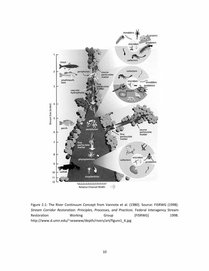
The river continuum concept (RCC) (Figure 2.1) proposed by Vannote et. al. (1980) attempt to

explain a continuous gradient of physical conditions from source to mouth within a river system.

It also indicated that structures of biotic communities and functional characteristics are adapted

in function of energy inputs along the river (e.g. organic matter). So, the RCC offers a probable

composition in its functional feeding groups FFG, for example, at headwater, the organisms are

dominated by shredders as the organic matter debris are bigger, and collectors due to food source

as fine particulate organic matter (FPOM) from fragmented leafs (coarse particulate organic

matter (CPOM)) within a river ecosystem (Vannote et. al.,1980). The RCC was conceived based

on “existing data” from geomorphology, hydrology, biogeography, and natural history (Resh and

Kobzina 2003). The RCC defines a unidirectional transport of materials and organisms in

watercourses resulting in longitudinal variations along the stream gradient (Barquin and Death

2011; Minton et al., 2008). It predicts biotic diversity from little streams to big rivers (Dettmers et

al., 2001). Furthermore, RCC indicates that changes in physical conditions and food availability in

rivers leads to a longitudinal pattern of macroinvertebrates and fishes conditioning the trophic

group compositions of aquatic community (Ibanñez et al 2009; Wolff el al. 2013). However,

Dettmers et al., (2011) indicated that the RCC predicts a highest diversity in rivers of middle order

(4–6) but does not predict arrangements for fishes of large rivers (>6th order).

The longitudinal arrangements within the stream ecosystems in the RCC are dominant in early

ecological studies (Lamberti et al., 2010) producing a new paradigm and motivating a good deal

of discussion (Resh and Kobzina 2003). The RCC is widely applied in many studies. Wolff el al.

(2013) found that fish assemblages follow the pattern expected by the River continuum concept.

It was also used to describe the freshwater-saltwater interface in estuarine ecosystems (Dame et

al., 1992), the zooplankton in a reservoir, river and estuary pathway (Akopian et al. 2002) and the

bacterial diversity along the river (Savio et al., 2015). The RCC was also employed to investigate

the gradient in infection level produced by fish parasites (Blasco-Costa et al., 2013), to predict

linear gradients in two fish species (Schaefer et al., 2011) and quantified phenotypic gradients in

freshwater snails (Minton et al., 2008). From a water basin protection perspective, Saunders et

al. (2002) indicated that following the RCC, headwater streams are more vulnerable to changes in

land use as a result of changes in energy input. On the other hand, downstream riparian

9

vegetation is required for shading, smoothing hydrological fluctuation, regulating nutrient loads

and avoiding erosion.

Nevertheless, Newson and Newson (2000) found that macroinvertebrate biological patterns

respond to longitudinal zonation like the RCC, but there is a noticeable secondary indicator

controlled by local habitat patterns. In addition, Greathouse and Pringle (2006) indicated that

macroinvertebrates distribution in a tropical island normally follow RCC however, additional

studies are needed to polish the influence of functional feeding groups distribution caused by

trophic regulators. Furthermore, Covich et al. (2009) indicated that the RCC do not consider

impediment related with neither sloped basin nor dissimilarities between streams that controls

predation and macroinvertebrate spreading. The RCC also considers a strong influence of coarse

particulate organic matter (CPOM) from terrestrial sources as primary energy input on headwater,

whereas downstream internal production rises generating its own energy sources (Saunders et al.

2002).

Additionally, some deviations to the RCC are found in literature. In a comparison between tropical

and temperate fish assemblages, Ibañez et al. (2009) found some differences in the expected

predictions of the RCC that can be linked to differences in energy availability between temperate

and tropical systems. Covich et al. (2009) indicated that for a diadromous shrimp, complexity in

tropical insular drainages combined with temporal variability and land use induces dissemination

and abundance of this shrimp in tropical stream ecosystems, which do not meet the RCC. They

also stated that geomorphic obstacles can influence the plenty of shrimps and impede the

spreading of their predatory fishes (Covich el al., 2009).

Blanco et al. (2013) found that in short coastal streams (1 to 10 km) do not follow the principles

of the RCC because of the steep gradient and the presence of waterfalls and cascades. Thus is

consistent with the typology observed in volcanic oceanic islands in the Caribbean and the Pacific.

They also indicated that low order (<3) streams usually ended on the sea quickly. Thus, periphyton

production and transportation debris is avoided. Downstream, riparian vegetation have mainly

shredders (specially shrimps) spreading along the stream. This is contrary to the RCC, which

expects shredders (mostly insects) mainly in headwater (Blanco et al., 2013).

10

Figure 2.1: The River Continuum Concept from Vannote et al. (1980). Source: FISRWG (1998).

Stream Corridor Restoration: Principles, Processes, and Practices. Federal Interagency Stream

Restoration Working Group (FISRWG) 1998.

http://www.d.umn.edu/~seawww/depth/rivers/art/figure1_4.jpg

11

2.4 Impacts of pollution

Pollution could be defined as any change in the characteristics of a natural environment that may

affect the normal behavior of living organisms (Morse et al., 2017). Impacts of environmental

pollution are related with health risk through food safety (Lu et al., 2015) and negative distresses

on water usage such as drinking, bathing or fishing (Gosset et al., 2016). Furthermore, pollution

of freshwater is considered one of the major manmade origin of global change in biota (Gonzalo

and Camargo 2013).

Pollution in freshwater systems have been studied. For instance, pollution due to artificial salinity

caused by anthropogenic activities affects the ecology of freshwater macroinvertebrates

(Cañedo-Argüelles et al., 2012). Pollution produced by pesticides and sediment induced by rainfall

event were investigated in order to quantify pollution (Dabrowski et al., 2002; Schulz, 2001), and

to determine the effect on biota (Thiere and Schulz 2004) in South-African rivers. Chemical

pollution was also studied in Iberian river basins. Kuzmanović et al. (2016) found that it is

negatively linked to river macroinvertebrates.

Pollution of watercourses in developing countries is mainly produced by exploitation of natural

resources (Da Silva and Sacomani 2001) but also is caused by fecal contamination and inorganic

compounds from natural or anthropogenic sources (Shah et al., 2007). In Malaysia, the major

sources of pollution in aquatic environment are domestic sewage and animal wastes. There are

also an increase of toxic and hazardous waste through the application of pesticides as well as the

development of industries and urbanization (Abdullah 1995).

Land use

The land use affects watercourses in different ways, which produce various complications on

water ecosystems and water quality (Bu et al., 2014). Differences are found by comparing water

quality parameters from diverse water catchments (Shah et al., 2007). Urban and industrial land

uses are associated with heavy metals, nutrients and organic pollutions while agriculture is linked

with nutrients (Bu et al., 2014). Recently studies were made to understand the relation between

land use and streams. (Ding et al., 2016; Bu et al., 2014). Ding et al. (2016) determined that minor

water quality was linked with cropland, orchard and grassland in highland catchments while it was

connected with biggest urban areas in the lowland catchments. Furthermore, Ding et al., (2016)

showed that the river suffered organic and nutrients pollution and regions controlled by

cultivated and urbanized land uses in the river basin have a tendency to have poorer water quality

than other zones.

Some studies associate agricultural land use to bad freshwater quality mainly induced by the

presence of pesticides. Chemical pollution as a result of agricultural activities are brought from

soil surface to the stream via runoff (Dabrowski et al., 2002; Schulz 2001; Thiere and Schulz 2004),

increasing the quantities of nitrogen and phosphorous in surface waters (Bu et al., 2014).

Pesticides negatively affect aquatic organisms including macroinvertebrates (Dabrowski et al.,

12

2002; Thiere and Schulz, 2004). Thiere and Schulz (2004) determined that pesticides and turbidity

exerted a great pressure on macroinvertebrate community.

Urbanization/wastewater

The growth of urbanization produced great impact on aquatic environments especially by

transporting substantial concentration of micro and macro pollutants by rainwater runoff. Diverse

kind of pollutants like Poly Aromatic Hydrocarbons (PHCs), heavy metals, poly-chlorobiphenols

(PCBs), pesticides, bacteria and others has been detected in streams. Because of these mixed

composition of urban rainwater runoff, the diversity of organisms is disturbed (Gosset et al.,

2016).

Other problem found in urban areas are misconnections of sewage that produce extra discharges

and polluted surface water (Revitt and Ellis, 2016; Ellis and Butler, 2015). Gosset et al. (2016)

indicated that environmental effect of discharges cannot be anticipated only with

physicochemical studies, it is necessary to combine them with biological indices and

ecotoxicological studies.

Impacts of dams

Dams are assumed to affect negatively stream biota. (Singer and Gangloff, 2011; Gonzalo and

Camargo 2013; Mbaka and Schaefer 2016). It is considered as the main threat by altering habitat

and reducing chances for several river fish (Mazumder et al. 2016). Furthermore, hydrological

modifications degrade freshwater ecosystems and could cause biodiversity losses, increment of

watercourse temperatures, affectation in the structure and functioning of freshwater community

(Castello and Macedo, 2016). Bredenhand and Sanways (2009) described that disturbance caused

by dams have a result in the loss of local biodiversity. Glowacki, et al. (2011) found that

Chironomids declined their diversity in upstream of reservoir and amplified in downstream of it,

while the contrary happen to fish. However, Singer and Gangloff (2011) found that some small

dams improves conditions for freshwater mussel growth downstream. Mbaka and Schaefer

(2016) state that small impoundments has a slight effect on biota and could need minor attention

than other stressors.

13

3. MATERIALS AND METHODS

3.1. Study area

The Portoviejo River basin is located in the coastal central area of Manabí province (Thielen et al

2016). It covers an area of 2108.29 km2 (Macías and Díaz, 2010). Within the basin, Poza-Honda

reservoir is located which is 12 km in length and covers an area of 6 km2. It was built to provide

irrigation and drinking water. Water drains to the Pacific Ocean with an average discharge of 11

m3/s recorded on 2013 (INAMHI (b), 2015). The zone has two marked seasons, the rain season

starts on December and finish on April or May. The rest of the year is the dry season with almost

no precipitation occurs, excluding the years when El Niño phenomenon occurs (INAMHI, 2015).

Average precipitation within the basin is 1334 mm recorded on 2012 (INAMHI (a), 2015).

In total, thirty-one sites were sampled (Fig. 3.1), three within the reservoir (Poza Honda), five in

small tributary streams, twenty-two sites were along the Portoviejo river, the main river of the

basin, and one was sampled in the estuarine system. The sites were selected based on accessibility

and along a pollution gradient. Three sites were considered as pristine which served as reference

sites.

Figure 3.1: Map of study area in the Portoviejo River with indications of sampling sites.

Portoviejo river starts after the dam and runs along 152 km passing the cities of Santa Ana and

Portoviejo. The Santa Ana canton has a population of 47,385 inhabitants (INEC, 2010) in which

14

20% of the population are residing in the urban area of 1000 km2. On the other hand, the

Portoviejo canton has an extension of 968 km2 and a population of 280,029 inhabitants (INEC,

2010). The Portoviejo city has 72% of the total population of the Portoviejo canton, which means

there are 201,620 inhabitants in an area of 32 km2.

Fifty percent of the Portoviejo canton is a conservation area. Eighteen percent is an agricultural

area for cultivating corn, cocoa, coffee, plantain, rice, coconut, lemon, peanuts, cassava, pearl

onions, sugarcane, tomato kidney, sweet pepper, bean, melon, watermelon, papaya, mango,

passion fruit, cucumber, badea, higuerilla and achiote and some others fruits. Cattle pastures

constitute fourteen percent while anthropogenic use (urban area and others) is four percent

forest comprises nine percent while the rest of the territory is for other uses (MAGAP, 2012).

There are 645 inhabitants at the upstream of the dam. Most of the land is covered by forest, but

small portions of the land are cultivated with coffee, cocoa, lemon, orange, banana, tagua palm,

plantain, yucca, tree beans and papaya, peanuts, yucca and beans and cattle are also pastured.

3.2 Data collection

3.2.1 Macroinvertebrates

Sampling campaign was directed during July and August, 2015. Macroinvertebrates were

collected by kick sampling method using a standard conical hand net with a frame size of 20×30

cm and a mesh size of 500 µm, attached to a stick as specified by Gabriels et al. (2010). Each

sampling site was sampled for 5 min. along a 10-20 m segment. Sampling effort was uniformly

distributed over all aquatics habitats at the sampling site including stones, sands or mud,

macrophytes and others natural or artificial substrates. In addition, macroinvertebrates were also

picked by hands from stones, logs and leaves. Macroinvertebrates were sorted alive and identified

at family level.

3.2.2. Physicochemical characteristics

At each sample site, physicochemical data were collected. Temperature, specific conductivity,

chlorophyll, water pH and turbidity were measured by using multiprobes YSI-6600 while dissolved

oxygen (DO) and dissolved oxygen saturation (DOsat) were measured by multiprobes YSI-6920.

Both probes were submerged in a bucket with approximate 10 liters of water sample. Data was

recorded over several minutes per location. The final values were obtained by calculating the

average of the last 15 recorded measurements. Chemical oxygen demand (COD), total nitrogen

(Total N), total phosphorous (Total P), orthophosphate-P, nitrate-N (NO3--N), nitrite-N (NO2

--N),

ammonium-N (NH4+-N), biological oxygen demand (BOD) and total organic carbon (TOC) were

measured ex situ. For each sampling site, water samples were taken and stored in a cool and dark

container. The samples were analysed in the laboratory using Hach-Lange spectrophotometer

kits. Average water velocity were measured with the flow meter model höntzsch HFA, Höntzsch

GmbH manufacturer.

15

3.2.3. Hydromorphological characteristics

For each sampling site, mean and maximum depth of the water body, average and maximum

width of the river, floodplain and flood prone width, sludge layer were measured manually.

Furthermore, the type of watercourse, land use surrounding each bank (10 x 100 m), shading,

abundance of macrophytes, presence of water hyacinth, valley form, channel form, profile of the

bank, extent of bank erosion, type of bank material, bank shape, bank slope, variation in flow,

variation in width, presence of dead wood, pool-riffle class, types of mineral substrates, sediment

type, bed compaction, sediment matrix and sediment angularity were estimated through field

inspection. Additionally, sampling site elevation were recorded using GPS Garmin eTrex®30. An

overview of the classes of each of these variables can be found in Appendix A.

3.3. Chemical and ecological assessment

3.3.1. Chemical indices

In this study, the chemical water quality was determined with The Dutch method and LISEC

method.

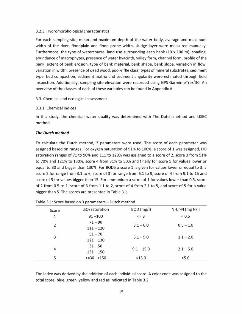
The Dutch method

To calculate the Dutch method, 3 parameters were used. The score of each parameter was

assigned based on ranges. For oxygen saturation of 91% to 100%, a score of 1 was assigned, DO

saturation ranges of 71 to 90% and 111 to 120% was assigned to a score of 2, score 3 from 51%

to 70% and 121% to 130%, score 4 from 31% to 50% and finally for score 5 for values lower or

equal to 30 and bigger than 130%. For BOD5 a score 1 is given for values lower or equal to 3, a

score 2 for range from 3.1 to 6, score of 3 for range from 6.1 to 9, score of 4 from 9.1 to 15 and

score of 5 for values bigger than 15. For ammonium a score of 1 for values lower than 0.5, score

of 2 from 0.5 to 1, score of 3 from 1.1 to 2, score of 4 from 2.1 to 5, and score of 5 for a value

bigger than 5. The scores are presented in Table 3.1.

Table 3.1: Score based on 3 parameters – Dutch method

Score %O2 saturation BOD (mg/l) NH4+-N (mg N/l)

1 91 –100 <= 3 < 0.5

2 71 – 90

3.1 – 6.0 0.5 – 1.0 111 – 120

3 51 – 70

6.1 – 9.0 1.1 – 2.0 121 – 130

4 31 – 50

9.1 – 15.0 2.1 – 5.0 131 – 150

5 <=30 –>150 >15.0 >5.0

The index was derived by the addition of each individual score. A color code was assigned to the

total score: blue, green, yellow and red as indicated in Table 3.2.

16

Table 3.2: Water quality assessment according to Dutch Method

Class Color code Score Quality

1 blue 3 – 4.5 Excellent, very pure

2 green 4.6 – 7.5 Good, pure

3 yellow 7.6 – 10.5 Moderate, doubtful

4 orange 10.6 – 13.5 Bad, polluted

5 red 13.6 - 15 Very bad, heavily polluted

The LISEC method

The LISEC method was derived using 4 parameters, one variable more than the Dutch method.

For LISEC index orthophosphate was used with a score of 1 for values lower or equal to 0.05, a

score of 2 from 0.5 to 0.25, score of 3 from 0.25 to 0.9, score of 4 from 0.9 to 1.5 and score of 5

for values bigger or equal to 1.5. The parameters and scores are presented in Table 3.3.

Table 3.3: Score system based on 4 parameters – LISEC method

Score %O2 saturation BOD (mg/l) NH4+-N (mg N/l) t.an. PO4

3-P (mg P/l)

1 91 –100 <= 3 < 0.5 <= 0.05

2 71 – 90

3.1 – 6.0 0.5 – 1.0 <0.05 - <0.25 111 – 120

3 51 – 70

6.1 – 9.0 1.1 – 2.0 0.25 - <0.90 121 – 130

4 31 – 50

9.1 – 15.0 2.1 – 5.0 0.90 - <1.50 131 – 150

5 <=30 –>150 >15.0 >5.0 <= 1.5

Individual scores were summed. A color code was assigned to the total score: blue, green, yellow

and red as indicated in Table 3.4.

Table 3.4: Water quality assessment according to LISEC method

Class Color code SUM score Quality

1 Blue 4 – <6 Excellent, very pure

2 Green 6 – <10 Good, pure

3 Yellow 10 – <14 Moderate, doubtful

4 Orange 14 – <18 Bad, polluted

5 Red 18 – 20 Very bad, heavily polluted

3.3.2. Ecological indices

The ecological quality of each site was assessed with Biological Monitoring Working Party adapted

for Colombia (BMWP-Col, Alvarez, 2005). The BMWP-Col was used since it is considered an

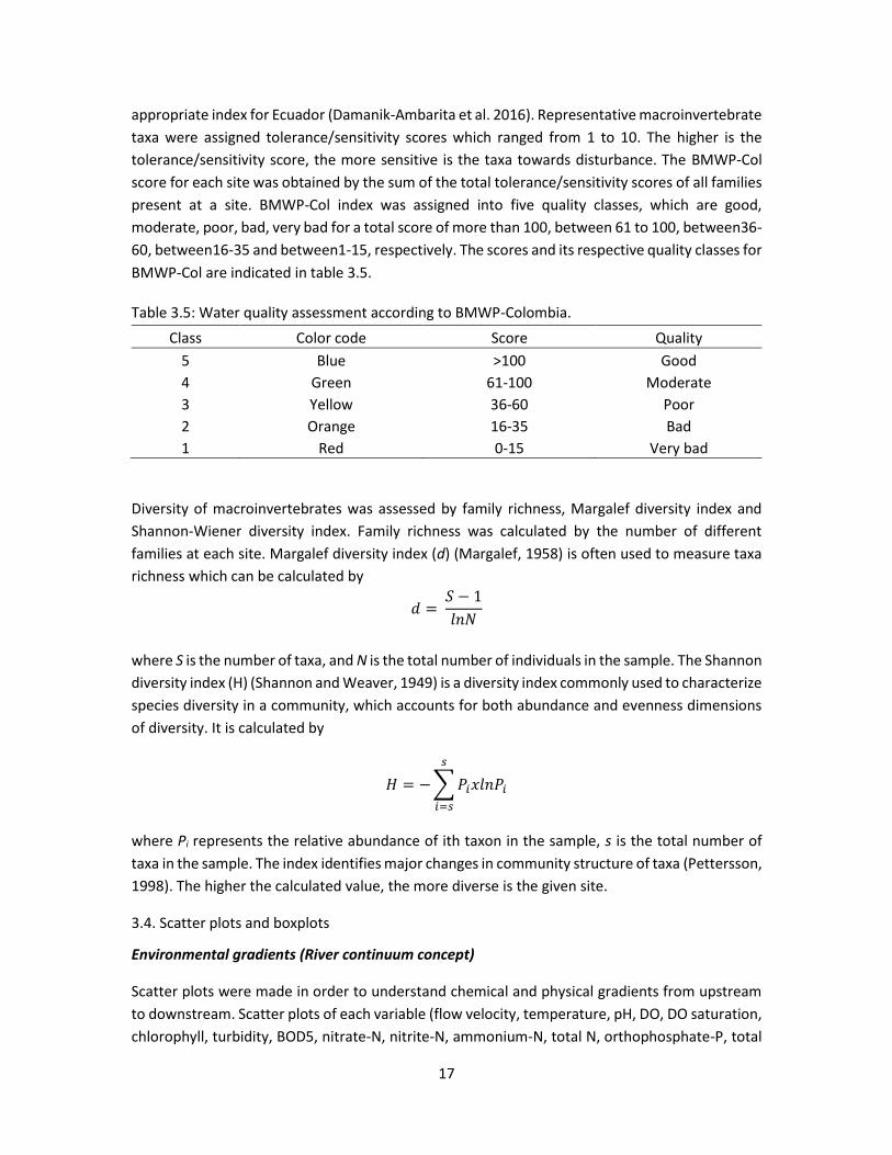
17

appropriate index for Ecuador (Damanik-Ambarita et al. 2016). Representative macroinvertebrate

taxa were assigned tolerance/sensitivity scores which ranged from 1 to 10. The higher is the

tolerance/sensitivity score, the more sensitive is the taxa towards disturbance. The BMWP-Col

score for each site was obtained by the sum of the total tolerance/sensitivity scores of all families

present at a site. BMWP-Col index was assigned into five quality classes, which are good,

moderate, poor, bad, very bad for a total score of more than 100, between 61 to 100, between36-

60, between16-35 and between1-15, respectively. The scores and its respective quality classes for

BMWP-Col are indicated in table 3.5.

Table 3.5: Water quality assessment according to BMWP-Colombia.

Class Color code Score Quality

5 Blue >100 Good

4 Green 61-100 Moderate

3 Yellow 36-60 Poor

2 Orange 16-35 Bad

1 Red 0-15 Very bad

Diversity of macroinvertebrates was assessed by family richness, Margalef diversity index and

Shannon-Wiener diversity index. Family richness was calculated by the number of different

families at each site. Margalef diversity index (d) (Margalef, 1958) is often used to measure taxa

richness which can be calculated by

𝑑 = 𝑆 − 1

𝑙𝑛𝑁

where S is the number of taxa, and N is the total number of individuals in the sample. The Shannon

diversity index (H) (Shannon and Weaver, 1949) is a diversity index commonly used to characterize

species diversity in a community, which accounts for both abundance and evenness dimensions

of diversity. It is calculated by

𝐻 = − ∑ 𝑃𝑖𝑥𝑙𝑛𝑃𝑖

𝑠

𝑖=𝑠

where Pi represents the relative abundance of ith taxon in the sample, s is the total number of

taxa in the sample. The index identifies major changes in community structure of taxa (Pettersson,

1998). The higher the calculated value, the more diverse is the given site.

3.4. Scatter plots and boxplots

Environmental gradients (River continuum concept)

Scatter plots were made in order to understand chemical and physical gradients from upstream

to downstream. Scatter plots of each variable (flow velocity, temperature, pH, DO, DO saturation,

chlorophyll, turbidity, BOD5, nitrate-N, nitrite-N, ammonium-N, total N, orthophosphate-P, total

18

P, TOC, percent predators, percent scrapers, percent collectors, percent scrapers, percent

odonates) were plotted in function of the distance from the mouth to determine the change of

each variable from upstream to downstream.

Ecological quality and environmental variables

Boxplots of each BMWP-Col class as a function of each environmental variable (flow velocity,

temperature, pH, DO, DO saturation, chlorophyll, turbidity, BOD5, nitrate-N, nitrite-N,

ammonium-N, total N, orthophosphate-P, total P and TOC) were plotted to relate the impacts of

these variables on ecological water quality. Furthermore, boxplots of BMWP-Col scores were built

in function of each hydromorphological variable (type of watercourse, land use, shading,

macrophytes abundance, water hyacinth presence, valley form, channel form, profile of the bank,

bank erosion, bank material, bank shape, bank slope, variation in flow, variation in width , dead

wood, pool-riffle class, types of mineral substrates, sediment type, bed compaction, sediment

matrix and sediment angularity) to compare the relation between BMWP-Col and these variables.

Impacts of land use, dams, and waste water treatment plant (WWTP)

Boxplots of each land use class in function of each environmental variable (flow velocity,

temperature, pH, DO, DO saturation, chlorophyll a, turbidity, BOD5, nitrate-N, nitrite-N,

ammonium-N, total N, orthophosphate-P, total P and TOC) and BMWP-Col were made to compare

the impacts of land uses. The impact of dams was also determined. Boxplots of each dam category

(before dam, after dam, reference sites, and other impacted sites) in function of each

environmental variable and BMWP-Col were built. To assess the effect of waste water treatment

plants (WWTP), boxplots of each WWTP class (before the WWTP, after the WWTP, reference sites,

and other impacted sites) were made in function of each environmental variables and BMWP-Col.

3.5. Data analysis

All statistical analysis and plots were made in R Software (R Core Team, 2016). As the software’s

language is easy to apply in syntax with many built-in statistical functions and excellent graphical

capabilities (Verzani, 2002).

The non-parametric “Kruskal-Wallis rank-sum test" was implemented to determine if there is a

difference of means in each environmental variable among each land use, dam and WWTP

category. Kruskal-Wallis rank-sum test can be viewed as the generalization of the Wilcoxon rank-

sum test for more than two groups. Kruskal-Wallis was used to assess the hydrological and

anthropogenic influence in the reservoir in Ethiopia (Ambelu et al. 2013) and the influences of

environmental factor on macroinvertebrates in Zimbabwe (Dalu et al., 2012). Furthermore, to

assess. the differences of means among each group (category), a pairwise post-hoc comparison

of means by Wilcoxon rank-sum test was performed

19

4. RESULTS

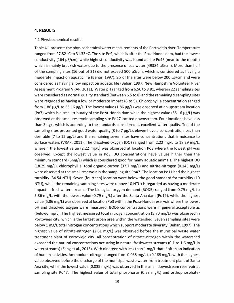
4.1 Physicochemical results

Table 4.1 presents the physicochemical water measurements of the Portoviejo river. Temperature

ranged from 27.82 ◦C to 31.33 ◦C. The site Po9, which is after the Poza Honda dam, had the lowest

conductivity (164 µS/cm), while highest conductivity was found at site Po46 (near to the mouth)

which is mainly brackish water due to the presence of sea water (49384 µS/cm). More than half

of the sampling sites (16 out of 31) did not exceed 500 µS/cm, which is considered as having a

moderate impact on aquatic life (Behar, 1997). Six of the sites were below 200 µS/cm and were

considered as having a low impact on aquatic life (Behar, 1997; New Hampshire Volunteer River

Assessment Program VRAP, 2011). Water pH ranged from 6.50 to 8.81, wherein 22 sampling sites

were considered as normal quality standard (between 6.5 to 8) and the remaining 9 sampling sites

were regarded as having a low or moderate impact (8 to 9). Chlorophyll a concentration ranged

from 1.86 µg/L to 55.16 µg/L. The lowest value (1.86 µg/L) was observed at an upstream location

(Po7) which is a small tributary of the Poza-Honda dam while the highest value (55.16 µg/L) was

observed at the small reservoir sampling site Po47 located downstream. Four locations have less

than 3 µg/L which is according to the standards considered as excellent water quality. Ten of the

sampling sites presented good water quality (3 to 7 µg/L), eleven have a concentration less than

desirable (7 to 15 µg/L) and the remaining seven sites have concentrations that is nuisance to

surface waters (VRAP, 2011). The dissolved oxygen (DO) ranged from 2.22 mg/L to 18.29 mg/L,

wherein the lowest value (2.22 mg/L) was observed at location Po3 where the lowest pH was

observed. Except the lowest value in Po3, DO concentrations have values higher than the

minimum standard (5mg/L) which is considered good for many aquatic animals. The highest DO

(18.29 mg/L), chlorophyll a, total organic carbon (37.7 mg/L) and nitrite-nitrogen (0.143 mg/L)

were observed at the small reservoir in the sampling site Po47. The location Po11 had the highest

turbidity (34.54 NTU). Seven (fourteen) location were below the good standard for turbidity (10

NTU), while the remaining sampling sites were (above 10 NTU) is regarded as having a moderate

impact in freshwater streams. The biological oxygen demand (BOD5) ranged from 0.79 mg/L to

5.86 mg/L, with the lowest value (0.79 mg/L) after the Santa Ana dam (Po19), while the highest

value (5.86 mg/L) was observed at location Po3 within the Poza-Honda reservoir where the lowest

pH and dissolved oxygen were measured. BOD5 concentrations were in general acceptable as

(below6 mg/L). The highest measured total nitrogen concentration (5.70 mg/L) was observed in

Portoviejo city, which is the largest urban area within the watershed. Seven sampling sites were

below 1 mg/L total nitrogen concentrations which support moderate diversity (Behar, 1997). The

highest value of nitrate-nitrogen (2.81 mg/L) was observed before the municipal waste water

treatment plant of Portoviejo city. All concentration of nitrate-nitrogen within the watershed

exceeded the natural concentrations occurring in natural freshwater streams (0.1 to 1.6 mg/L in

water streams) (Zang et al., 2016). With nineteen with less than 1 mg/L that if often an indication

of human activities. Ammonium-nitrogen ranged from 0.035 mg/L to 0.185 mg/L, with the highest

value observed before the discharge of the municipal waste water from treatment plant of Santa

Ana city, while the lowest value (0.035 mg/L) was observed in the small downstream reservoir at

sampling site Po47. The highest value of total phosphorus (0.53 mg/L) and orthophosphate-

20

phosphorus (0.33 mg/L) were observed in a downstream location at the confluence of Portoviejo

river and Rio Chico river, which is the second large stream within the river basin. With exception

of sampling site Po3, total phosphorus exceeds the minimum allowed concentration (0.05 mg/L)

which is considered as potential nuisance concentration for freshwater ecosystems (VRAP, 2011).

Table 4.1. Mean, median, maximum and minimum of physicochemical variables measured in the Portoviejo river basin.

Variables Unit Mean Median Maximum Minimum

Temperature ◦C 27.69 27.82 31.33 25.56

Conductivity µS/cm 2445.30 425.00 49384.00 164.00

pH - 7.88 7.87 8.81 6.50

Chlorophyll a µg/L 13.28 7.17 55.16 1.86

Dissolved oxygen mg/L 7.97 7.71 18.29 2.22

Dissolved oxygen demand-sat. % 102.75 98.31 243.18 28.29

Turbidity NTU 15.06 14.22 34.54 0.00

Chemical oxygen demand mg/L 9.29 3.00 142.00 *3.00

Biological oxygen demand mg/L 3.00 2.82 5.86 0.79

Total nitrogen mg/L 1.77 1.20 5.70 *0.50

Total phosphorus mg/L 0.23 0.21 0.53 *0.05

Nitrate-nitrogen mg/L 1.02 0.53 2.81 *0.23

Nitrite-nitrogen mg/L 0.0372 0.0260 0.1430 *0.0015

Ammonium-nitrogen mg/L 0.085 0.079 0.185 0.035

Orthophosphate-phosphorus mg/L 0.20 0.20 0.33 *0.05

Total organic carbon mg/L 15.99 17.00 37.70 *3.00

Flow velocity m/s 0.38 0.44 0.88 0.00

Elevation m 59.06 59.00 121.00 3.00

Distance from the mouth Km 82.53 93.22 138.24 0.45

*Values expressed as the detection limit of the kit

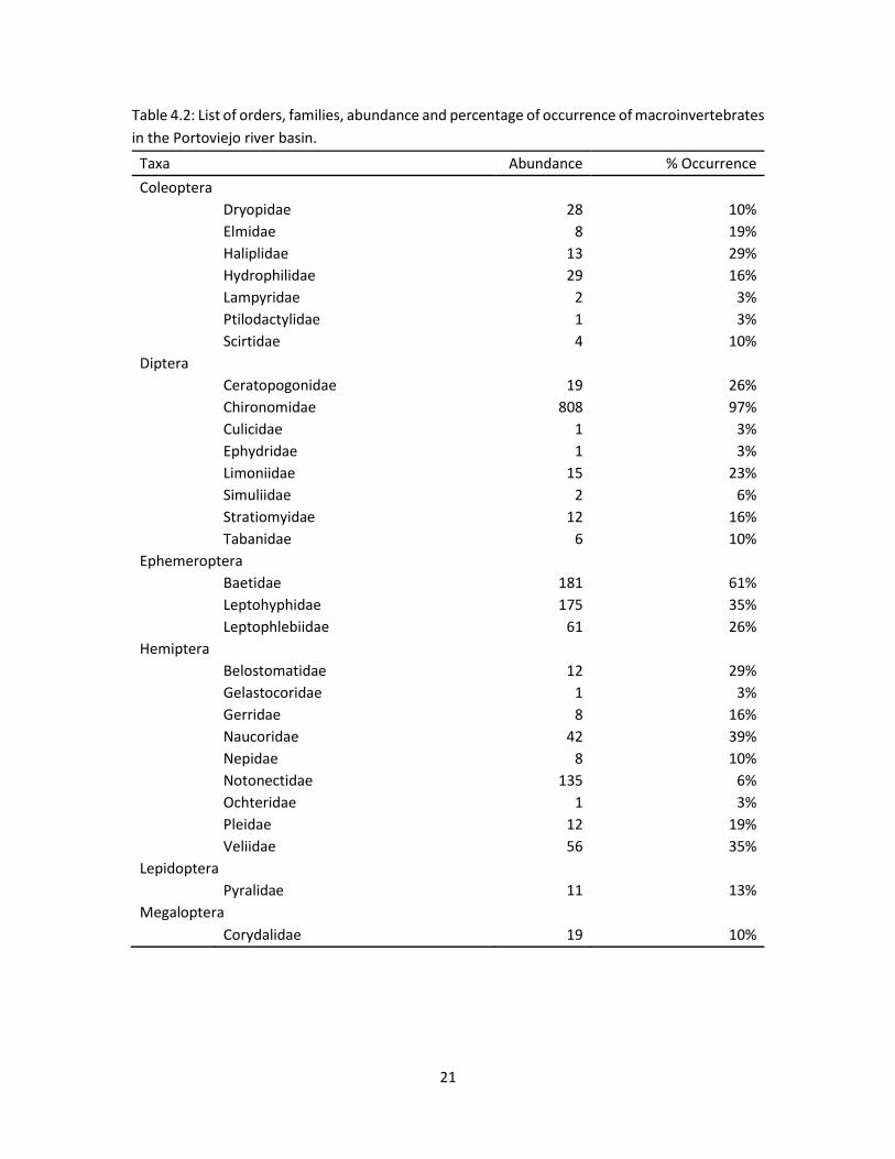
4.2. Macroinvertebrates

In total, more than 8000 macroinvertebrates of 54 different families were sorted and identified.

The highest richness was observed in a small tributary of the main river with 22 families. The

insect constituted the highest number of families (39 out of 54 families), with Hemiptera, Diptera,

Coleoptera and Trichoptera (9, 8, 7 and 5 families respectively) as the main orders. Chironomidae

occurred most frequently, succeeded by Coenagrionidae, Libellulidae and Baetidae at 30, 21, 20

and 19 sites, respectively. Thiaridae was the most abundant family, followed by Chironomidae,

Corbiculidae and Libellulidae (5231, 808, 247 and 231 individuals respectively). Table 4.2 shows

the list of orders, families, abundance and percentage of occurrence encountered in the

Portoviejo river basin.

21

Table 4.2: List of orders, families, abundance and percentage of occurrence of macroinvertebrates

in the Portoviejo river basin.

Taxa Abundance % Occurrence

Coleoptera

Dryopidae 28 10%

Elmidae 8 19%

Haliplidae 13 29%

Hydrophilidae 29 16%

Lampyridae 2 3%

Ptilodactylidae 1 3%

Scirtidae 4 10%

Diptera

Ceratopogonidae 19 26%

Chironomidae 808 97%

Culicidae 1 3%

Ephydridae 1 3%

Limoniidae 15 23%

Simuliidae 2 6%

Stratiomyidae 12 16%

Tabanidae 6 10%

Ephemeroptera

Baetidae 181 61%

Leptohyphidae 175 35%

Leptophlebiidae 61 26%

Hemiptera

Belostomatidae 12 29%

Gelastocoridae 1 3%

Gerridae 8 16%

Naucoridae 42 39%

Nepidae 8 10%

Notonectidae 135 6%

Ochteridae 1 3%

Pleidae 12 19%

Veliidae 56 35%

Lepidoptera

Pyralidae 11 13%

Megaloptera

Corydalidae 19 10%

22

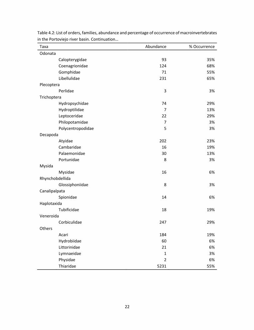
Table 4.2: List of orders, families, abundance and percentage of occurrence of macroinvertebrates

in the Portoviejo river basin. Continuation…

Taxa Abundance % Occurrence

Odonata

Calopterygidae 93 35%

Coenagrionidae 124 68%

Gomphidae 71 55%

Libellulidae 231 65%

Plecoptera

Perlidae 3 3%

Trichoptera

Hydropsychidae 74 29%

Hydroptilidae 7 13%

Leptoceridae 22 29%

Philopotamidae 7 3%

Polycentropodidae 5 3%

Decapoda

Atyidae 202 23%

Cambaridae 16 19%

Palaemonidae 30 13%

Portunidae 8 3%

Mysida

Mysidae 16 6%

Rhynchobdellida

Glossiphoniidae 8 3%

Canalipalpata

Spionidae 14 6%

Haplotaxida

Tubificidae 18 19%

Veneroida

Corbiculidae 247 29%

Others

Acari 184 19%

Hydrobiidae 60 6%

Littorinidae 21 6%

Lymnaeidae 1 3%

Physidae 2 6%

Thiaridae 5231 55%

23

4.3 Water Quality Indices

The water quality score for all 31 sampling sites based on BMWP-Col (Roldán, 2003) ranged from

16 to 140 (Fig 4.1; Appendix B: Table B1). High scores were observed at sites with dissolved oxygen

concentrations between 7 and 9 mg/L, conductivity between 239 and 890 µg/L, a chlorophyll

concentration lower than or equal to 6 mg/L, a turbidity lower than 29 NTU, a flow velocity higher

than or equal to 0.56 m/s, water temperature between 25.8 and 26.2 °C, a thin sludge layer (less

than 5cm), the pH between 7.7 and 8.3, a biological oxygen demand lower than 3.1 mg/L, total

nitrogen lower than or equal to 1.3 mg/L, total phosphorus lower than 2.4 and a total organic

carbon content lower than or equal to 13.4 mg/L. All physicochemical variables are presented in

Appendix B: Table B2. Sites with tightly packed bed, filled contact matrix and a well-rounded

sediment angularity were associated with high BMWP-Col score. The site with highest BMWP-Col

score had gravel bed bank substrate. Boxplots are presented in Appendix C: Fig. C1 to Fig. C5. High

BMWP-Col values were perceived at locations where the number of taxa was also the high

(between 20 and 22 taxa).

Figure 4.1: Map showing BMWP-Col quality classes of sampling sites in Portoviejo river basin.

The Margalef's diversity index (Margalef, 1958) ranged from 0.7708 to 3.9550 (Fig. 4.2a ; Appendix

B: Table B1) and Shannon Wiener diversity index (Shannon and Weaver, 1949) ranged from

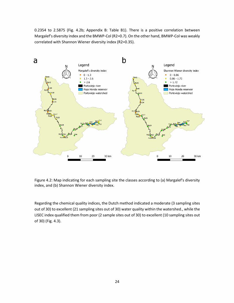
24

0.2354 to 2.5875 (Fig. 4.2b; Appendix B: Table B1). There is a positive correlation between

Margalef’s diversity index and the BMWP-Col (R2=0.7). On the other hand, BMWP-Col was weakly

correlated with Shannon Wiener diversity index (R2=0.35).

Figure 4.2: Map indicating for each sampling site the classes according to (a) Margalef's diversity index, and (b) Shannon Wiener diversity index.

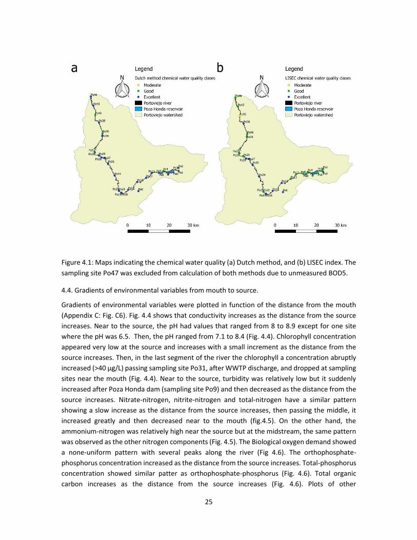
Regarding the chemical quality indices, the Dutch method indicated a moderate (3 sampling sites

out of 30) to excellent (21 sampling sites out of 30) water quality within the watershed., while the

LISEC index qualified them from poor (2 sample sites out of 30) to excellent (10 sampling sites out

of 30) (Fig. 4.3).

25

Figure 4.1: Maps indicating the chemical water quality (a) Dutch method, and (b) LISEC index. The

sampling site Po47 was excluded from calculation of both methods due to unmeasured BOD5.

4.4. Gradients of environmental variables from mouth to source.

Gradients of environmental variables were plotted in function of the distance from the mouth

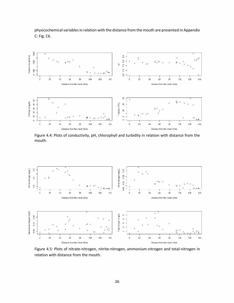
(Appendix C: Fig. C6). Fig. 4.4 shows that conductivity increases as the distance from the source

increases. Near to the source, the pH had values that ranged from 8 to 8.9 except for one site

where the pH was 6.5. Then, the pH ranged from 7.1 to 8.4 (Fig. 4.4). Chlorophyll concentration

appeared very low at the source and increases with a small increment as the distance from the

source increases. Then, in the last segment of the river the chlorophyll a concentration abruptly

increased (>40 µg/L) passing sampling site Po31, after WWTP discharge, and dropped at sampling

sites near the mouth (Fig. 4.4). Near to the source, turbidity was relatively low but it suddenly

increased after Poza Honda dam (sampling site Po9) and then decreased as the distance from the

source increases. Nitrate-nitrogen, nitrite-nitrogen and total-nitrogen have a similar pattern

showing a slow increase as the distance from the source increases, then passing the middle, it

increased greatly and then decreased near to the mouth (fig.4.5). On the other hand, the

ammonium-nitrogen was relatively high near the source but at the midstream, the same pattern

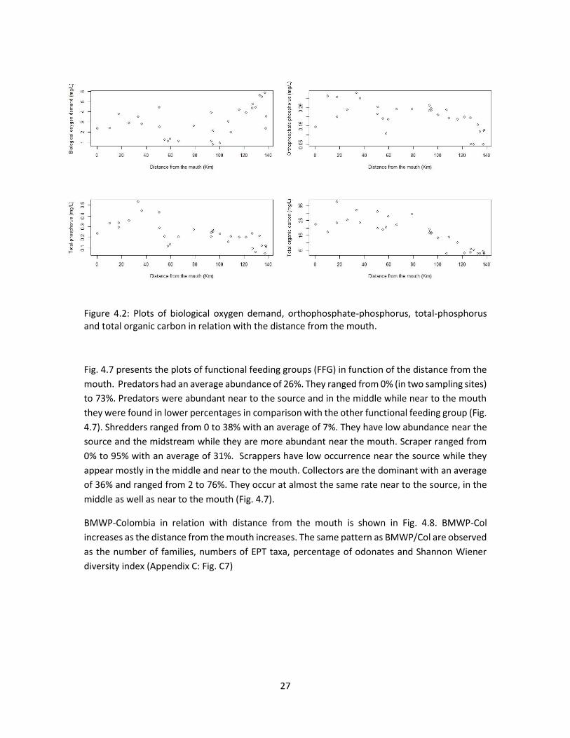
was observed as the other nitrogen components (Fig. 4.5). The Biological oxygen demand showed

a none-uniform pattern with several peaks along the river (Fig 4.6). The orthophosphate-

phosphorus concentration increased as the distance from the source increases. Total-phosphorus

concentration showed similar patter as orthophosphate-phosphorus (Fig. 4.6). Total organic

carbon increases as the distance from the source increases (Fig. 4.6). Plots of other

26

physicochemical variables in relation with the distance from the mouth are presented in Appendix

C: Fig. C6.

Figure 4.4: Plots of conductivity, pH, chlorophyll and turbidity in relation with distance from the mouth.

Figure 4.5: Plots of nitrate-nitrogen, nitrite-nitrogen, ammonium-nitrogen and total-nitrogen in

relation with distance from the mouth.

27

Figure 4.2: Plots of biological oxygen demand, orthophosphate-phosphorus, total-phosphorus and total organic carbon in relation with the distance from the mouth.

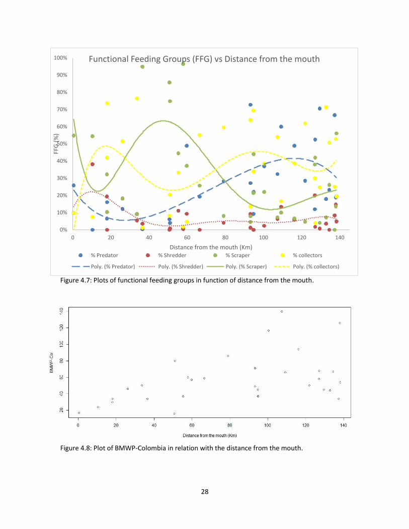
Fig. 4.7 presents the plots of functional feeding groups (FFG) in function of the distance from the

mouth. Predators had an average abundance of 26%. They ranged from 0% (in two sampling sites)

to 73%. Predators were abundant near to the source and in the middle while near to the mouth

they were found in lower percentages in comparison with the other functional feeding group (Fig.

4.7). Shredders ranged from 0 to 38% with an average of 7%. They have low abundance near the

source and the midstream while they are more abundant near the mouth. Scraper ranged from

0% to 95% with an average of 31%. Scrappers have low occurrence near the source while they

appear mostly in the middle and near to the mouth. Collectors are the dominant with an average

of 36% and ranged from 2 to 76%. They occur at almost the same rate near to the source, in the

middle as well as near to the mouth (Fig. 4.7).

BMWP-Colombia in relation with distance from the mouth is shown in Fig. 4.8. BMWP-Col

increases as the distance from the mouth increases. The same pattern as BMWP/Col are observed

as the number of families, numbers of EPT taxa, percentage of odonates and Shannon Wiener

diversity index (Appendix C: Fig. C7)

28

Figure 4.7: Plots of functional feeding groups in function of distance from the mouth.

Figure 4.8: Plot of BMWP-Colombia in relation with the distance from the mouth.

0%

10%

20%

30%

40%

50%

60%

70%

80%

90%

100%

0 20 40 60 80 100 120 140

FFG

(%

)

Distance from the mouth (Km)

Functional Feeding Groups (FFG) vs Distance from the mouth

% Predator % Shredder % Scraper % collectors

Poly. (% Predator) Poly. (% Shredder) Poly. (% Scraper) Poly. (% collectors)

29

4.5. Impacts of dams

Boxplots were made to examine the impact of dams in the Portoviejo river (Fig. 4.9). The non-

parametric Kruskal-Wallis rank-sum test indicated that flow velocity, pH, dissolved oxygen and

chlorophyll in the Portoviejo river basin significantly differed between references, other impacts

(different from a dam), before a dam and after a dam sampling sites (p-value < 0.05) Appendix B:

Table B3. Boxplot shows that pH has differences from at least one categorical sampling site. A

pairwise post-hoc comparison of means by using Wilcoxon rank-sum tests indicated that pH

before a dam is significantly different than the other impacted sites. However, pH has no

significant difference among the remaining clusters. A significant difference in dissolved oxygen

content was observed among the clustered sampling sites (chi-squared = 13.968, df = 3, p-value

= 0.003; Kruskal-Wallis). The DO concentration at the impacted sampling sites (other than dams)

was significantly different from the reference, before a dam and after a dam sampling sites. There

were no significant differences in the DO concentration between remaining clusters. Flow velocity

(chi-squared = 7.900, df = 3, p-value = 0.048; Kruskal-Wallis) is significantly higher at impacted

sampling sites (other than dams) than in sites before a dam (Fig. 4.9). There are no significant

differences of flow velocities between remaining clusters. The chlorophyll content (chi-squared =

8.574, df = 3, p-value = 0.036; Kruskal-Wallis) is significantly low at reference sampling sites than

in sites with impacted sampling sites. There were no significant differences in the chlorophyll

content between remaining clusters (Fig. 4.9).

Figure 4.9: Boxplot of velocity, pH, dissolved oxygen and chlorophyll-a in relation with impacts

produced by the presence of a dam Reference, other, before, after refers to pristine site, sites

impacted by other activities, sites before dams(reservoir), sites after the dams, respectively.

30

On the other hand, water quality parameters such as temperature, conductivity, turbidity, COD,

BOD5, Nitrate-nitrogen, nitrite-nitrogen, ammonium-nitrogen, total-nitrogen, orthophosphate-

phosphorus, total-phosphorus and total organic carbon does not differ significantly between the

clustered sampling sites. The boxplot of these variables in relation with impact of a dam are

presented in Appendix C: Fig. C8 and Fig. C9.

Regarding to chemical indices, both the Dutch method and LISEC index are significantly different

among clustered sampling sites. (p-value <0.05). (chi-squared = 8.1886, df = 3, p-value = 0.04227

and chi-squared = 8.6666, df = 3, p-value = 0.03407 respectively). Dutch method and LISEC index

have significantly high score in before the dam sites than in other impacted sampling sites. There

were no significant differences in score of Dutch method and LISEC index among other clustered

sampling sites

Figure 4.10: Boxplot of Dutch method and LISEC index in relation with impacts produced by the

presence of a dam. Reference, other, before, after refers to pristine site, sites impacted by other

activities, sites before dams (reservoir), sites after the dams, respectively.

Additionally, BMWP-Col, number of families, percentage of odonates, Margalef’s diversity index

and Shannon Wiener diversity index does not differ significantly between clustered sampling sites

(Appendix Table C3). Moreover, numbers of EPT (Ephemeroptera, Plecoptera and Trichoptera)

taxa differ significantly between clustered sampling sites (chi-squared = 9.546, df = 3, p-value =

0.02285; Kruskal-Wallis). EPT taxa in reference sampling sites were significantly higher than other

impacted sampling sites. There were no significant differences in numbers of EPT taxa among

other clustered sampling locations. Appendix C Figure C10.

31

4.6. Impact of Land use

Boxplot in Fig. 4.11, 4.12 and 4.13 shows physicochemical variables in relation with land use. The

Kruskal-Wallis test presented in Table 4.3 indicates that the distance from the mouth, flow

velocity, chlorophyll, conductivity, turbidity, biological oxygen demand, nitrate-nitrogen, nitrite-

nitrogen, total-nitrogen, orthophosphate-phosphorus, total-phosphorus and total organic carbon

in the Portoviejo river basin significantly differed between forest, agriculture and residential land

uses (p-value < 0.05). The flow velocity in the forest land use is significantly lower from flow

velocity in arable land use. There were no significant differences in flow velocities among other

land uses. Chlorophyll concentration shows significant differences among land uses (Fig. 4.9). The

chlorophyll a concentration in forest was significantly lower from residential areas. None of the

other land uses show a difference in chlorophyll a concentration at 5% significance level. The

boxplot of conductivity shows differences in land uses (Fig. 4.9), which is confirm by Kruskal-Wallis

test (Table 4.3). It was observed that conductivity in forest was lower than arable land use and

residential areas. There were no significant differences in conductivity between arable and

residential areas. Boxplot in Fig. 4.10 shows differences in turbidity between land uses. The

average turbidity in forest was lower than on the arable land and residential areas. There were

no significant differences between the average turbidity in arable zones and residential areas. The

boxplots indicate differences in the average of 5 days’ biological oxygen demand between forest,

arable and residential land uses. The average BOD5 in forest was higher than in arable areas and

in residential areas while there was no difference between arable and residential areas (fig 4.10).

Total organic carbon shows differences in concentrations among land uses. Total organic carbon

concentrations were lower in forest than arable and residential areas (Fig. 4.11). Nitrate-nitrogen

concentration was significantly difference among different land uses. Figure 4.10 shows that

nitrate-nitrogen concentration is lower in forest zones than in residential and arable areas

(confirmed by a pairwise comparison), while no differences were observed between residential

and arable areas. Boxplots shows differences between nitrite-nitrogen concentrations between

land uses. Nitrite-nitrogen were lower in forest areas than in arable and residential areas (Fig.

4.10). There was no difference between arable and residential land use. Boxplots in Fig. 4.11

indicated differences in the total nitrogen concentrations between land uses. The average total

nitrogen concentration in forest areas is significantly lower than in residential area. There were

no differences in total nitrogen concentration between forest and residential nor between arable

and residential areas. There were some differences in orthophosphate-phosphorus concentration

regarding land uses (fig. 4.11). The orthophosphate-phosphorus and total phosphorus

concentration were lower in forest areas than in arable land and residential zones. (Fig. 4.11).

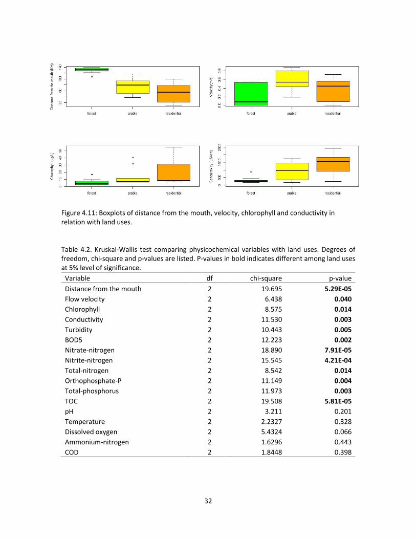
32

Figure 4.11: Boxplots of distance from the mouth, velocity, chlorophyll and conductivity in relation with land uses. Table 4.2. Kruskal-Wallis test comparing physicochemical variables with land uses. Degrees of freedom, chi-square and p-values are listed. P-values in bold indicates different among land uses at 5% level of significance.

Variable df chi-square p-value

Distance from the mouth 2 19.695 5.29E-05

Flow velocity 2 6.438 0.040

Chlorophyll 2 8.575 0.014

Conductivity 2 11.530 0.003

Turbidity 2 10.443 0.005

BOD5 2 12.223 0.002

Nitrate-nitrogen 2 18.890 7.91E-05

Nitrite-nitrogen 2 15.545 4.21E-04

Total-nitrogen 2 8.542 0.014

Orthophosphate-P 2 11.149 0.004

Total-phosphorus 2 11.973 0.003

TOC 2 19.508 5.81E-05

pH 2 3.211 0.201

Temperature 2 2.2327 0.328

Dissolved oxygen 2 5.4324 0.066

Ammonium-nitrogen 2 1.6296 0.443

COD 2 1.8448 0.398

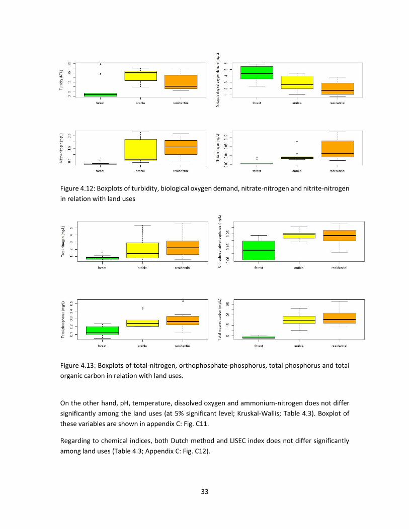
33

Figure 4.12: Boxplots of turbidity, biological oxygen demand, nitrate-nitrogen and nitrite-nitrogen

in relation with land uses

Figure 4.13: Boxplots of total-nitrogen, orthophosphate-phosphorus, total phosphorus and total

organic carbon in relation with land uses.

On the other hand, pH, temperature, dissolved oxygen and ammonium-nitrogen does not differ

significantly among the land uses (at 5% significant level; Kruskal-Wallis; Table 4.3). Boxplot of

these variables are shown in appendix C: Fig. C11.

Regarding to chemical indices, both Dutch method and LISEC index does not differ significantly

among land uses (Table 4.3; Appendix C: Fig. C12).

34

In addition, BMWP-Col, number of families, numbers of EPT taxa, percentage of odonates,

Margalef’s diversity index and Shannon Wiener diversity index does not differ significantly among

the land uses (at 5% significant level; Kruskal-Wallis; Table 4.3; Appendix C: Fig. C13).

4.7 Effect of municipal waste water treatment plants

Boxplot in Figure 4.14 indicates differences in turbidity among reference, before and after waste

water treatment plants (WWTP) and other impacts. It is confirming by Kruskal-Wallis test that

there were significant differences (chi-squared = 8.806, df = 3, p-value = 0.03; Kruskal-Wallis). A

post-hoc analysis indicated significant difference in turbidity between references sampling sites

and other impacted sampling sites (5% of significant level). There were no significant differences

between references and before municipal waste water treatment plant, nor between reference

sampling sites and after municipal waste water sampling sites, in the same way the other

comparisons show no significant differences.

Figure 4.14: Boxplot of turbidity in relation with impacts caused by WWTP. Reference, other,

before, after refers to pristine site, sites impacted by other activities, sites before WWTP, sites

after the WWTP, respectively.

The other physicochemical variables such as velocity, temperature, pH, DO, chlorophyll, BOD5,

nitrogen, phosphorus compounds and TOC have no significant differences in relation with impacts

caused by waste water treatment plant (p value> 0.05; Kruskal-Wallis test) (Appendix B: Table

B4). Boxplots of these variables are shown in Appendix C: Fig. C14 and Fig. C15.

Concerning to chemical indices, both the Dutch method and LISEC index have no significant

differences in relation with the impacts caused by waste water treatment plant (p-value> 0.05;

Kruskal-Wallis test). Boxplots are shown in Appendix Figure C16.

35

On the other hand, BMWP-Col scores were significantly higher in references sampling sites than

sites impacted by other activities other than WWTP. There were no significant differences in

BMWP-Col scores between the remaining clusters (Figure 4.14). As similar as the former, numbers

of families and EPT taxa were significantly higher in references sampling sites than in sites

impacted by other activities. There were no significant differences in numbers of families and EPT

taxa between before and after WWTP and the remaining clusters. Moreover, Margalef’s diversity

index, Shannon Wiener diversity index and percentage of odonates do not differed significantly

among clustered impacts related to waste water treatment plant (Appendix C Table C4 and Figure

C18).

36

5. DISCUSSION

5.1 Water quality

The water of Portoviejo River is mainly used for irrigation, human consumption and recreation.

The Poza-Honda dam assures water availability during the dry season. Physicochemical water

quality in the river and within the reservoir is influenced by anthropogenic activity by settlements

nearby. Poza Honda reservoir and their tributaries, which is the upstream of the Portoviejo river

are considered as protected area by the national secretariat of water (Secretaria Nacional del

Agua SENAGUA). Due to limited human activities, a very low conductivity is expected. This is

similar to what was found in Abras de Mantequilla with conductivities lower than 35 µS/cm

(Alvarez et al. 2013). However, due to uncontrolled settlement and agricultural activities at the

upstream areas within the dam, the tributaries and the Portoviejo River had values closer to 500

µS/cm. In areas downstream of the Portoviejo River with human settlements and agricultural

activities, values higher than 900 µS/cm were recorded. This is in line with expected values within

areas with anthropogenic activities such as wastewater discharge (Damanik-Ambarita et al. 2016),

urbanization (Mereta et al. 2012), and run-off of pesticides (Prado et al. 2015) as a result of

agricultural activities in the Portoviejo river valley (INIAP, 2011). The highest conductivity value in

sampling site Po46 corresponds to estuarine system (Jun et al. 2016). High concentrations of

chlorophyll-a (translated in phytoplankton abundance) found downstream could be caused by

untreated wastewater. Those sampling sites are located after the inlet of the municipal waste

water treatment plant of Portoviejo city which were also characterized by nutrient enrichment

(NO3--N, NO2--N, Total N and Total P). Most of the sampling sites had Dissolved Oxygen (DO)

concentration higher than 5 mg/L except site Po3 which is located within the dam, with a DO

concentration of 2.22 mg/L. This value in site Po3 could be due to higher oxygen consumption as

confirmed with high BOD5 (5.86 mg/L) measurement. This is due to the dense presence of water

hyacinth (up to 75%) which avoid the contact of water with wind and the degradation of dead

water hyacinth, and shading produced by trees on the vicinity which avoid sunlight in the water

column that avoid oxygen production by aquatic plants. Total nitrogen concentration in upstream

areas is in average higher than the values reported by Alvarez et al. (2013) in Abras de

Mantequilla. However, values lower than 1 mg/L were recorded that are considered good enough

to support moderate diversity life (Behar, 1997). This total nitrogen concentration could be

produced by organic matter loads from natural sources as indicated by Bustamante et al. (2015)

that occurs in South America’s rivers. While in downstream areas the total nitrogen content

exceeded the proposed guideline for drinking water (Devic et al. 2014). This load could be due to

agricultural runoff from numerous small inputs over a wide area (Zevallos, 2002; INIAP, 2011), or

from fecal pollution in no sewer settlements (WHO, 1996) that are present in the zone. The

highest concentration of phosphorus content, reported in Po36 (0.53 mg/L), due to the presence

of septic systems, sewage, animal waste and fertilizer along Portoviejo and Rio Chico river, which

merge in site Po36 (Zevallos, 2002). However, the highest total phosphorus concentration is below

the standards for drinking water by WHO (1993). Nitrate-nitrogen were below the detection limit

(0.23 mg/L) of the chemical kits within the Poza Honda reservoir and their tributaries and nitrite-

nitrogen were lowest than 0.003 mg/L is in line with values found by Alvarez et al., (2013). Whilst

37

ammonium-nitrogen concentration in the same zone was higher than the maximum values found

in wetlands and rivers in Abras de Mantequilla (Alvarez et al, 2013). On the other hand,

concentrations of nitrate-nitrogen, nitrite-nitrogen and ammonium-nitrogen measured in the

other sampling sites in Portoviejo river were lower than concentrations recommended for

drinking water use (WHO, 2011). In general, the lower concentrations recorded indicate that there

was no eutrophication in the Portoviejo river despite of presence of settlements and cultivation

in their riparian zone. Turbidity in upstream areas within the Poza Honda dam and tributaries was

very low (>5 NTU) which means that in upstream zones the amount of suspended material in the

water, such as algae, silt and clay, suspended sediment and decaying plant material was very low.

While passing the Poza Honda dam the turbidity was higher initially caused by sediments that are

carried out from the bottom of the reservoir due to the configuration of the tunnel (bottom

tunnel) and the bank erosion that introduce suspended material in the water column.

Based on BMWP-Colombia, a good ecological quality status in Portoviejo river is associated with

flow velocities, low temperatures, low conductivity, low chlorophyll-a content, low BOD5 and low

nutrient concentrations. Good quality status is better in upstream areas that have lesser human

impact areas. This is in line with results found by Alvarez et al., (2013) in Abras de Mantequilla.

However, a bad water quality was found in sampling site Po3 within the reservoir where the

lowest DO content and pH and highest BOD5 were measured. On the other hand, bad quality

classes downstream are related to urbanization and possible input of untreated domestic

wastewater, similar to values found downstream by Damanik-Ambarita et al. (2016) in the Guayas

river basin. Regarding to the hydro-morphological variables, high BMWP-Colombia scores were

observed in sampling sites with gravel bank material and gravel mineral substrate. This in line with

Lemes da Silva et al. (2016) who explained that grain particle size composition is determinant for

macroinvertebrate taxonomic richness and density. Furthermore, Niba and Mafereka (2015)

indicated that substrate is important in defining species dissemination pattern.

Based on BMWP-Colombia the ecological quality ranged from good to bad, while based on the

Dutch method and LISEC index, water quality ranged from moderate to excellent, indicating

differences in classification between biotic and abiotic water quality indices. Higher diversity and

higher number of EPT taxa in Portoviejo river were associated with good quality of BMWP-Col.

Damanik-Ambarita et al. (2016) indicates that high diversity and sensitive taxa are good water

quality indicators. High scores of Margalef's diversity index and Shannon Wiener diversity index

were calculated on sampling sites with good quality classes based on BMWP-Col (Table C.1).

5.2 River continuum/ Gradients from source to mouth

Sampling sites located at upstream areas generally has low human impacts. As we expected, near

to the source is forested area, followed by arable land and residential areas at the middle and

lastly residential areas near to the mouth. In general, an increase of conductivity, chlorophyll a,

available nutrients (e.g. total nitrogen and total phosphorus) and total organic carbon was

detected from source to downstream areas. Studies have shown that levels of conductivity can

increase in freshwater due to urbanization (Mereta et al. 2012). Furthermore, nutrient levels in

38

freshwater can increase due to the use of chemical fertilizer in riverine (Damanik-Ambarita et al.

2016) which also allow phytoplankton increment and hence an increase of chlorophyll a.

On the other hand, turbidity near to the source is relatively low as a result of the presence of trees

at the riparian zone which avoid erosion of the banks. Then, turbidity increased just right after

the dam due to sediments brought from the bottom of the dam by the bottom tunnel of Poza

Honda dam and by erosion of the riverine. As the distance from the source increases, less trees

are present in the riverine zone due to the shift of land use into agricultural areas. However,

turbidity increase along the downstream zone of the river. This in concordance to the results of

Sherriff et al. (2015) who indicated that agriculture activities could accelerate erosion of the soil.

The BOD5 near the source is relatively higher than downstream. This could be as the result of

degradation of organic matter from decaying leaves and organic material from sewage of

settlements near the brooks that discharge water to the main river. At the middle, the BOD5

decreases showing relatively low values. This could be the result of sewage system which avoid

inputs of organic matter in this part of the river. At the downstream of the river, the BOD5

increases probably due to effluents of untreated sewage directly to the river. Most of the sampling

sites have a DO concentration between 5 to 12 mg/L. Relatively high values were measured

upstream near the source until the middle (between 7 to 12 mg/L), except sampling site Po3

within the reservoir which has a DO concentration of 2.22 mg/L, the lowest pH (6.5) and the

highest BOD (5.86 mg/L). This low DO could be explained by accumulation of decaying leafs.

Relatively low values are found near the mouth with exception of sampling site Po47 which has

the highest DO concentration (18.29 mg/L). This value could be the result of oxygen

oversaturation by photosynthesis of aquatic plants (e.g. phytoplankton) since the highest value of

chlorophyll a (55.16 µg/L) was measured in that sampling site. With the exception of sites Po3 and

Po47, a decreasing trend in DO concentration occurs from source to the mouth.

In general, BMWP-Col scores increases as the distance from the mouth increases. This pattern

indicates that near the source, water quality is better than near to the mouth due to less

anthropogenic activity which influence species richness (Céréghino et al. 2003). This results are in

line with those in the Guayas river basin by Damanik-Ambarita et al. (2016) who indicated that

rivers upstream have better quality status due to lesser anthropogenic activities, while

downstream it affects negatively the water quality. The same pattern is shown by richness and

diversity indices (e.g. numbers of families, numbers of EPT taxa, percentage of odonates,

Margalef’s index and Shannon Wiener). The high diversity and the sensitive taxa are indication of

good water quality in upstream areas.

Regarding to functional feeding groups (FFG), predators and collectors are the dominant

upstream. While at the middle, scrapers are relatively high in percentage. Near to the mouth,

collectors are dominant (Fig. 4.7). From the river continuum concept (Vannotte et al) shredders

and collectors are the dominants at upstream areas due to presence of available food such as

leaves from trees and fine particulate organic matter (FPOM) from fragmented leafs. While

grazers and predators are present in relatively lower percentages. However, in Portoviejo river,

shredders have the lowest percentage in upstream areas. This result could be explained due to

39

predation which is high numbers of predators at the upstream. This plenty of predators could be

due to absence of natural predators (e.g. fish) of macroinvertebrate predators as indicated by

Covich el al. (2009) who stated that geomorphic obstacles (e.g. dam) can influence the abundance

of these macroinvertebrates predators and impede the presence of predatory fishes. Collectors

and scrapers in upstream areas are in line with the expectation from the RCC. At the middle,

scrapers are the dominant in the Portoviejo river. While collectors and predators tend to decrease

and shredders have the lowest percentages. Thus, in line with predictions of the RCC at midstream

the expected high percentage of scrapers is accomplished mainly due to food availability (e.g.

periphyton and biofilm), and low percentage of shredders because at midstream is expected that

most of the leaves are already consumed by shredders near to the mouth (Vannote et al.,1980).

However, contrary to RCC which expected collectors to be the dominant at midstream, at the

midstream of the Portoviejo river, collectors have percentage lower than scrapers. As expected

from RCC, collectors are dominant near the mouth in the Portoviejo river. Collectors feed on

FPOM which is found in this part of the river. On the other hand, scraper and shredder are present

in lower percentage than collectors. However, the RCC indicates that near to the mouth nearly no

shredders are found as leaves were already consumed by shredders near to the source and in the

middle, and limited or no grazers are expected. The presence of shredder near to the mouth could

be explained by the presence of some trees in the banks, which are not dominant regarding to

land use but enough to bring leaves to the river, while scraper could eat periphyton and biofilm

on surface of stones, vascular hydrophytes or sediments. As expected, predators are present in

low percentage near to the mouth. Furthermore, the differences found in our research are in line

with Ibañez et al., (2009) who found some differences in the expected predictions of the RCC due

to differences in energy availability between temperate and tropical systems and could the

presence of dam be also a reason as explained by Covich el al. (2009).

5.3 Impacts

5.3.1 Impact causes by dams in Portoviejo river

Damming causes changes in the natural flow regimen and could affect negatively stream

ecosystems (Gonzalo and Camargo 2013). The first evident change was the flow velocity after and

before a dam. Water pH after dams is lower than before dams probably due to the presence of

sediment or accumulation of decaying material. Findings of Mwedzi et al. (2016) indicated that

dissolved oxygen concentration in sampling sites downstream of impoundments is lower than in

non-dammed sites. Contrarily, in the Portoviejo river, dissolved oxygen (DO) concentration in

other non-dammed sampling sites was lower than in the reference, before a dam and after a dam

sampling sites. There are no significant differences in DO concentrations between after a dam and

before a dam sampling sites. Other physicochemical variables measured in the Portoviejo river

have no significant downstream effects probably because the dam has small impoundments,

which is in concordance with Mbaka et al. (2015) who indicate that in small impoundments does

not significantly change physicochemical parameters. Furthermore, Mendoza-Lera et al. (2012)

found negligible alteration in physicochemical variables due to presence of reservoirs. However,

from boxplots (Fig. C8) a decrease in temperature trend and an increase trend in turbidity can be

40

reported. Temperature reduction is due to the heat exchange with the air caused by the water

flow. Turbidity increment could be explained by the presence of sediments dragged from the

bottom of the dam due to the configuration of the tunnel (bottom tunnel) in the Poza Honda

reservoir (SENAGUA, 2015).

The Dutch method and LISEC index have higher scores before dams indicating bad water chemical

status comparing to sampling sites after dams, reference and other impacted sampling sites.

Contrary to what was stated above that dams have minimal impact on chemical parameters other

than flow, temp, DO, turbidity, with the LISEC or DUCTH method, it shows differences. So, based

on those indices, dams affect negatively freshwater quality. This means that the effect is more

pronounced when chemical parameters are taken together such as done in LISEC or DUTCH

method than when looking at the chemical parameters separately.

Wang et al. (2013) observe reduction on richness and EPT taxa as a result of flow regulation

caused by dams. On the contrary, there were no significant differences found in richness and EPT

taxa after and before a dam in Portoviejo River (Fig. C10). In the same way, BMWP-Col, percentage

of odonates, Margalef’s diversity index and Shannon Wiener diversity index did not reflect

significant differences between after and before dams. Those results could be explained by the

finding of Brainwood and Burgin (2006) that indicated that species richness and abundance of

communities varied greatly between dams, influenced by water quality and habitat feature that

defined equilibrium conditions. As a result, local condition equilibrates macroinvertebrate

communities, affecting feeding groups rather than specific taxa (Brainwood and Burgin, 2006). On

the other hand, as we expected, references sampling sites possess better water quality than the

other clustered sampling sites, as these sites have low human impacts.

5.3.2 Impact of Portoviejo river cause by land use

Population growth and rapid urbanization of upstream riverine areas mean a threat to freshwater

ecosystems (De Troyer et al. 2016), which leads in changes in land use and generation of organic

pollution. A first observation is that forest area is located near the sources while arable land at

the middle and residential areas near to the mouth (Fig. 4.11) which is in line with the river

continuum (Vannote et al., 1980). Flow velocity are lower in forest areas, upstream of the river

due to the presence of the dam, and low in residential areas due to impairments to catch water,

while arable areas have relatively higher flow velocities due to the landscape which is more steep

in the midstream than in the upstream. The chlorophyll a is higher in residential areas than in

forest and in arable land, due to the input of nutrients from untreated domestic wastewater

(Kawasaky et al. 2009). Conductivity and nutrients (e.g. Phosphorus and nitrogen) in forest areas

are relatively low compared with arable land. This can be due to the addition of pesticides and

nutrients in agricultural area as explained by Collins et al. (2013). High conductivity and nutrients

in residential areas can be due to inputs of decaying organic matter of human origin like found by

Kaup and Burgess (2002) in surface water. Conversely, BOD5 in forest areas is relatively higher

than in arable and residential zones. This could be explained by the leaf litters from the trees that

can be source of organic matter. Furthermore, BOD5 input from untreated domestic wastewater

41

that comes from settlements in forest areas that not possess sewage systems which are

discharged in the brooks that reach the main river. Similar findings are observed by Scheren et al.

(2000) who found domestic BOD loads in the Lake Victoria in Kenya. In addition, physicochemical

indices (e.g. Dutch method and LISEC index) present no significant differences between land uses.

In addition, biotic indices (e.g. BMWP-Col, number of families, numbers of EPT taxa, percentage

of odonates, Margalef’s diversity index and Shannon Wiener diversity index) are not significantly

different among land uses, in opposition to Mwedzi et al. (2016) who found that

macroinvertebrates in urban sites indicate severe pollution while in forested and farming sites

indicates relatively clean water. However, the BMWP/Col at the Portoviejo river with arable land

use has relatively higher scores than with forested area. This in contrast to Damanik-Ambarita et

al. (2016) who found that forested areas possess relatively higher scores than in arable land use

within the Guayas river basin. Those results could indicate that in arable land areas there is not

yet too much contamination to affect species sensitive to pollution. On the other hand, it is

possible that some degree of contamination influenced forested areas affecting those sensitive

to pollution species. This unexpected contribution to pollution in forested area could be explain

by inputs that come from settlements upstream which are brought by small brooks to the main

stream.

5.3.3 Effects of municipal wastewater treatment plant in the Portoviejo river basin

Among the physicochemical variables, turbidity is higher in sampling sites after and before WWTP

discharges. However, there is no significant difference in turbidity after and before WWTP

discharge which means that WWTP did not contribute to the variation in turbidity. The other

physicochemical variables are not statistically affected by the presence of a municipal WWTP.

Although, Fig. C15 shows that the chlorophyll a concentration after WWTP is relatively higher than

before WWTP, reference and other impacted sampling sites. Furthermore, the BOD5 after WWTP

is also relatively higher than before WWTP which could indicate an enrichment of organic waste

perhaps due to an insufficient removal of organic waste. Both chlorophyll a and BOD5 could be

an indication of insufficient treatment of wastewater or could be outflow due to low quantity of

wastewater that come to the WWTP at that specific time and it perhaps is release untreated. In

the same way, TOC and total phosphorus after WWTP are higher than before WWTP, while total

nitrogen after WWTP is relatively lower than before WWTP. However, reference sites indicated

less pollution mainly due to lesser anthropogenic disturbances.

Regarding to physicochemical indices, the boxplot of Dutch method (Fig. C18) shows lower score

which means that water quality after WWTP is relatively lower than other clustered sampling sites

while the LISEC index indicates that water quality is the same after and before WWTP. The

differences between both indices could be explained because the Dutch method used % oxygen

concentration, BOD5 and ammonium while LISEC index includes the variables included in Dutch

method and also orthophosphate-P to calculate the total score. Nevertheless, both (Dutch

method and LISEC index) have no significant variation between and among clustered sampling

sites with a relative better quality in reference sampling sites.

42

As expected, references sampling sites have better BMWP scores than the other clustered

sampling sites, mainly due to less anthropogenic activities at reference zones. BMWP-Col is not

significantly different between sites after and before municipal WWTP discharges. The same is

indicated by EPT taxa, Margalef’s diversity index, Shannon Wiener diversity index and percentage

of odonates. However, BMWP-Col scores before WWTP are relatively higher than after WWTP.

Similar results are observed with number of families and EPT taxa. This result indicates that

WWTPs is adding some degree of pollution reducing richness and diversity and affecting

sensitivities species used to calculated BMWP-Col scores. Maybe because the WWTP is not

efficient enough to remove pollution. Perhaps it helps as perhaps without it, water quality would

be worse. But maybe additional treatment is needed to fully treat the waste. Or maybe the load

is too much for the current WWTP that already exists. Those findings indicate that municipal

WWTP discharges affect the distribution and richness of macroinvertebrates in the Portoviejo

river.

43

6. CONCLUSIONS AND RECOMMENDATIONS

6.1 Conclusions

Ecological quality, expressed as BMWP-Colombia, classified majority of sampling sites at

Portoviejo River with a poor quality. This classification is associated to nutrient inputs from

agricultural areas. However, some upstream sampling sites were classified with good and

moderate status. In general, the good ecological quality is associated with high flow velocities,

low temperatures, low conductivity, low chlorophyll a content, low BOD5 and low nutrient

concentrations. Additionally, good water quality is also associated with the presence of sensitive

taxa and high diversity. On the other hand, some sampling sites were classified with bad quality,

mainly downstream sites, where the cumulative effects of pollution are present. Bad quality at

the downstream of the river is related to urbanization and inputs of untreated domestic

wastewater.

Locations near the source have lower pollution impact. In general, an increase in conductivity,

chlorophyll a, available nutrients, and total organic carbon was measure along the gradient from

source to the mouth. This is related to land use changes that come from forested areas upstream

of the river, passing an agricultural zone at the midstream and residential areas near the mouth.

DO decreases along the river gradient. Turbidity is low near the source but high at the middle due

to agriculture, then it tends to be low near to the mouth where residential areas are found. BOD

is high near to the source because the presence of decomposed leaf, decreases at the middle and

increase near to the mouth due to untreated sewage discharge. From the mouth to source, there

is a clear pattern of increasing scores of BWWP-Colombia. The same for richness and diversity

indices (e.g. numbers of families, numbers of EPT taxa, percentage of odonates, Margalef’s index

and Shannon Wiener). This indicates that upstream areas of Portoviejo River have better quality

status than downstream zones. There is an evolution of functional feeding groups (FFG) along the

gradient from source to the mouth. Predators and collectors are dominant upstream of the river.

While at the middle, scrapers are relatively high in percentage. Near to the mouth, collectors are

dominant. There is some deviation in the gradient predicted by the River Continuum Concept

(RCC). This deviation is explained by the presence of a series of dams along the river and also

differences in food availability between tropical systems and temperate zones where the concept

was started.

Dams affect freshwater ecosystems in different ways. Flow velocity, pH and temperature are low

before dams. While, turbidity is relatively high after dams. Other physicochemical variables

measured in the Portoviejo river have no significant effects at the downstream of dams. This

because, except the Poza Honda Dam, other dams present in the Portoviejo River are rather small.

However, more pronounced effects are found when chemical parameters are taken together (e.g.

LISEC and DUTCH indices). There were no significant differences found in biotic indices after and

before a dam in the Portoviejo River.

Gradients of land use are observed along the river. Forest is located in upstream areas, arable

land at the middle and residential zones near to the mouth. The chlorophyll a is higher in

44

residential areas than in forest and arable land. Conductivity and nutrients in forest areas are

relatively low compared with arable land. Conversely, BOD5 in forest areas is relatively higher

than in arable and residential zones. In addition, physicochemical indices (e.g. DUTCH method and

LISEC index) and biotic indices (e.g. BMWP-Col, number of families, numbers of EPT taxa,

percentage of odonates, Margalef’s diversity index and Shannon Wiener diversity index) are not

significantly different among residential zones, forested and agricultural land. However, BMWP-

Colombia has relatively higher scores at arable land than at forested area. This could be explained

by pollution input from settlements in upstream areas.

Physicochemical variables are not statistically affected by the presence of a municipal WWTP in

the Portoviejo River. Nonetheless, chlorophyll a, BOD5, TOC, total phosphorus and total nitrogen

after WWTP are relatively higher than before WWTP. Similar results are observed with BMWP-

Colombia, number of families and EPT taxa. Maybe because the WWTP is insufficient in organic

and nutrient removal or the load is more than the treatment plant can handle.

6.2 Recommendations.

A continuing monitoring to identify sources of pollution in the Portoviejo river is suggested.

Besides physicochemical monitoring, the ecological quality monitoring offers a tool to assess the

effects of pollution in the ecosystems. Thus, the BMWP-Colombia or other adaptations of

biological monitoring for Ecuadorians rivers is highly recommended to assess water quality in the

Portoviejo river. In the same way, knowledge about pollution gradients could help decision

makers to take actions to reduce the impacts of pollution along the river. However, in comparing

the River Continuum Concept, differences in tropical ecological communities, structures and

functions should be taken into account.

Although dams do not present serious effects within the Portoviejo River, its’ impacts on long

term and seasonality need to be studied in order to get better knowledge of the effects on

ecological ecosystem within the Portoviejo river. Changes in land use and pollution inputs

upstream should be controlled to avoid deterioration of the natural habitat along the riverine

zones. Actions to reduce changes in land uses and recuperation of natural vegetation within the

buffer zone in the riverine of Portoviejo River are necessary to reduce pollution. Since a great part

of the zone is used for agriculture, measurements of pesticides are suggested for future studies.

A revision of the efficiency and sufficiency of municipal Wastewater Treatment Plants is

suggested. Adaptations to the current configuration could be needed in order to avoid negative

impacts on water quality in the Portoviejo river.

45

REFERENCES

Abbasi, T.; Shahid A. Abbasi., 2012. Water quality indices. Elsevier. Printed in Great Britain.

Abdullah, A. R., 1995 Environmental pollution in Malaysia: trends and prospects. trends in analytical chemistry 14 (5)

Akkoyunlu, A.; Muhammed E. Akiner. 2012. Pollution evaluation in streams using water quality indices: A case study from Turkey’s Sapanca Lake Basin. Ecological Indicators 18, 501–511.

Akopian, M, Garnier, J, Pourriot, R. 2012. Zooplankton in an aquatic continuum: from the Marne River and its reservoir to the Seine Estuary. COMPTES RENDUS BIOLOGIES 325(7), 807-818.

Alabaster, J., Backiel, T., Hasselort, T., Lloid, R., Mitrovic, V., Dill, W., Throrslum, A., 1973. Water-quality criteria for European freshwater fish - report on ammonia and inland fisheries. Water research 7 (7), 1011-1022.

Alba-Tercedor J., 2000. BMWP’, un adattamento spagnolo del British Biological Monitoring Working Party (BMWP) Score System. Biologia Ambientale 14 (2), 65–67.

Alba-Tercedor J.; Jáimez-Cuéllar P.; Álvarez, M.; Avilés, J.; Bonada, N.; Casas, J, Mellado, A,; Ortega, M.; Pardo, I.; Prat, N.; Rieradevall, M.; Robles, S,; Sáinz-Cantero, C.E.; Sánchez-Ortega, A.; Suárez, M.L.; Toro,M.; Vidal-Albarca, M.R.; Vivas, S.; Zamora-Muñoz, C., 2004. Caracterización del estado ecológico de los ríos mediterráneos ibéricos mediante el índice IBMWP (antes BMWP’). Limnetica 21(3-4): 175–185.

Alvarez-Mieles, G.; Irvine, K.; Griensven, A. V.; et al., 2013. Relationships between aquatic biotic communities and water quality in a tropical river-wetland system (Ecuador). Environmental Science & Policy 34 (SI), 115-127.

Ambelu, A.; Lock, Koen, Goethals, Peter L.M. (2013) Hydrological and antropogenic influence in the Gilgel Gibe I reservoir (Ethiopia) on macroinvertebrates assemblages. Lake and reservoir management 29, 143-150.

Anonymous, 1969. Water quality criteria for European freshwater fish - water temperature and Inland fisheries. Water research 3 (9), 645.

Antonietti, R., 1996. Optimization of parameters used for freshwater survey. Water research 30 (6), 1535 -1538.

Armitage, P.; Moss, D.; Wright, J.; et al., 1983. The performance of a new biological water-quality score system based on macroinvertebrates over a wide-range of unpolluted running-water sites. Water research 17 (3), 333-347.

Azevedo, D. J. S.; Barbosa, J. E. L.; Gomes, W. I. A.; et al., 2015. Diversity measures in macroinvertebrate and zooplankton communities related to the trophic status of subtropical reservoirs: Contradictory or complementary responses? Ecological Indicators 50, 135-149.

Bagalwa, M., Majaliwa, M., Mushagalusa, N., & Karume, K. (2013). Estimation of transported pollutant load from small urban Kahuwa river micro-catchment in Lake Kivu, Democratic Republic of Congo. Journal of Environmental Science and Engineering. B, 2(8B), 460.

Barquin, J., Death, R., 2011. Downstream changes in spring-fed stream invertebrate communities: the effect of increased temperature range. Journal of Limnology 70(1), 134-146.

Barreto, L.; Fraga, M., Barros, F., et al., 2014. Relação entre vazão e qualidade da água em uma seção de rio. Relationship between stream flow and water quality in a river section. Revista Ambiente & Água 9 (1), 118-129.

46

Bartram, J., Ballance, R., 1996. Water Quality Monitoring. A practical guide to the design and implementation of freshwater quality studies and monitoring programmes, London, UK, Chapman & Hall.

Behar, S., 1997. Testing the Waters: Chemical and Physical Vital Signs of a River, Montpelier, VT, River Watch Network.

Beisel, J N ,Usseglio-Polatera, P ,Bachmann, V ,et al., 2003. A comparative analysis of evenness index sensitivity. International Review of Hydrobiology 88(1), 3-15.

Berger, E.; Peter Haase, MatthiasOetken, Andrea Sundermann., 2016. 1. Field data reveal low critical chemical concentrations for river benthic invertebrates. Science of the Total Environment 544, 864–873.

Bilotta, G. S.; Brazier, R. E.; Haygarth, P. M.; et al., 2008. Rethinking the contribution of drained and undrained grasslands to sediment-related water quality problems. Journal of environmental quality 37 (3), 906-914

Bilotta, G., and Brazier, R., 2008. Understanding the influence of suspended solids on water quality and aquatic biota. Water research 42 (12), 2849-2861.

Blanco, J., Escobar, C., & Carvajal, J., 2014. Gorgona, Baudó and Darién (Biogeographic Chocó, Colombia): model ecoregions for coastal stream ecology studies. Revista de Biología Tropical 62(1), 43-64.

Blasco-Costa, I.; Anson V. Koehler, Alice Martin And Robert Poulin., 2013. Upstream-downstream gradient in infection levels by fish parasites: a common river pattern. Parasitology 140, 266–274.

Brainwood, M. and Burgin, S., 2006. An exploration of relationships between macroinvertebrate community composition and physical and chemical habitat characteristics in farm dams. Environmental monitoring and assessment 19(1-3), 459-480.

Bredenhand, Emile, Sanways, Michael J., 2009. Impacts of a dam on benthic macroinvertebrates in a small river in a biodiversity hotspot: Cape Floristic Region, South Africa. Journal of insect conservation 13(3), 297-307.

Bu, Hongmei , Meng, Wei ,Zhang, Yuan ,et al., 2014. Relationships between land use patterns and water quality in the Taizi River basin, China. Ecological Indicators 41, 187-197.

Bustamante, M.; Martinelli L. A.; Perez, T.; et al., 2015. Nitrogen management challenges in major watersheds of South America. Environmental research Letters 10(6), Article number 065007.

Cañedo-Argüellesa, M.; Theodore E. Grantham, Isabelle Perrée, Maria Rieradevall, Raquel Céspedes-Sánchez, Narcís Prat. 2012. Response of stream invertebrates to short-term salinization: A mesocosm Approach. Environmental Pollution 166 ,144-151.

Cao, Y.; Bark, A.; Williams, W., 1997. Analysing benthic macroinvertebrate community changes along a pollution gradient: A framework for the development of biotic indices. Water research 31 (4), 884-892.

Carlisle, D. M.; Meador, M. R.; Moulton, S. R.; et al., 2007. Estimation and application of indicator values for common macroinvertebrate genera and families of the United States. Ecological Indicators 7 (1), 22-33.

Castello, L. and Macedo, M., 2016. Large-scale degradation of Amazonian freshwater ecosystems. Global Change Biology 22 (3), 990-1007.

Céréghino, R.; Young-Seuk Park, Arthur Compin and Sovan Lek, 2003. Predicting the species richness of aquatic insects in streams using a limited number of environmental variables. Journal of the North American Benthological Society 22 (3) , 442-456.

Chaoui, W., Bousnoubra, H., & Chaoui, K. (2013). Étude de la vulnérabilité à la pollution des eaux superficielles et souterraines de la région de Bouchegouf (Nord-Est Algérien). Nature & Technology, (8), 33B.

47

Charalampous, N.; Kindou, Aggeliki ,Vlastos, Dimitris ,et al., 2015. A Multidisciplinary Assessment of River Surface Water Quality in Areas Heavily Influenced by Human Activities. Archives of Environmental Contamination and Toxicology 69(2), 208-222.

Cicek, N. L.; Omer Osman ERTAN, 2012. Determination of the Water Quality of Köprüçay River (Antalya) According to the PhysicoChemical Parameteres. Ekoloji 21, 84, 54-65 (2012)

Collins, K.; Doscher, C.; Rennie, H.; et al., 2013. The effectiveness of riparian ‘restoration’ on water quality- A case study of lowland stream in Canterbury, New Zealand. Restoration ecology 21(1), 40-48.

Compin and Céréghino, R., 2003. Sensitivity of aquatic insect species richness to disturbance in the Adour–Garonne stream system (France). Ecological Indicators 3, 35–142.

Couto-Mendoza, M. t.; Vieira-Lanero R.; Cobo, F., 2014. More complexity does not always mean more accuracy: the case of IBMWP and METI in NW Spain. Ecohydrology. Ecohydrol.8, 595–609

Covich, A. P.; Todd A. Crowl, Catherine L. Hein, Mattj.Townsend and William H. Mcdowell., 2009. Predator–prey interactions in river networks: comparing shrimp spatial refugia in two drainage. Freshwater Biology 54(3):450 - 465

Da Silva, A.M.M. and Sacomani, L.B., 2001. Using chemical and physical parameters to define the quality of Pardo River water (Botucatu-SP-Brazil). Water research 35 (6), 1609-1616.

Dabrowski, J.; Sue K.C. Peall, Adriaan Van Niekerk, Adriaan J. Reinecke, Jenny A. Day, Ralf Schulz., 2002. Predicting runoff-induced pesticide input in agricultural sub-catchment surface waters: linking catchment variables and contamination.Water research 36, 4975–4984.

Dalu, T.; B. Clegg, T. Nhiwatiwa., 2012. Macroinvertebrate communities associated with littoral zone habitats and the influence of environmental factors in Malilangwe Reservoir, Zimbabwe. Knowledge and Management of Aquatic Ecosystems 406, 06.

Damanik-Ambarita, M. N.; Lock, K.; Boets, P.; et al., 2016. Water quality analysis of the Guayas river basin (Ecuador) based on macroinvertebrates indices. Limnologica 57, 27-59.

Dame, R., Childers, D. and Koepfler, E., 1992. A Geohydrologic Continuum Theory for the Spatial and Temporal Evolution of Marsh-Estuarine Ecosystems. Netherlands Journal of Sea Research 30, 63-72.

De Rosemond, S.; Duro, D. C.; Dube, M., 2009. Comparative analysis of regional water quality in Canada using the Water Quality Index. Environmental monitoring and assessment 156 (1-4), 223-240.

Debashis, Mazumder; Williams, Robert J., Wen, Li, et al., 2016. Impoundment constraint of fish niche diversity in a temperate Australian river. Hydrobiologia 771(1), 196-206.

DES 2015. Description of River Water Quality Parameters. http://des.nh.gov/. [Accessed 15 December 2015].

Dettmers, J., Wahl, D., Soluk, D. and Gutreuter. S., 2011. Life in the fast lane: fish and food web structure in the main channel of large rivers. Journal of the North American Benthological Society 20(2), 255-265.

Dietrich, J. P.; Ahna L. Van Gaest, Stacy A. Strickland, Mary R. Arkoosh., 2014. The impact of temperature stress and pesticide exposure on mortality and disease susceptibility of endangered Pacific salmon. Chemosphere 108, 353–359.

Ding, Jiao; Yuan Jiang, Qi Liu, Zhaojiang Hou, Jianyu Liao, Lan Fu, Qiuzhi Peng. 2016. Influences of the land use pattern on water quality in low-order streams of the Dongjiang River basin, China: A multi-scale analysis. Science of the Total Environment 551–552, 205–216.

EIFA-WP, 1969. Water quality criteria for European freshwater fish-extreme pH values and inland fisheries. European Inland Fishery Advisory commission Working Party (EIFA-WP) Water research 3 (8), 593-&

48

EIFA-WP, 1969. Water quality criteria for European freshwater fish-water temperature and inland fisheries. European Inland Fishery Advisory commission Working Party (EIFA-WP) Water research 3 (9), 645-&

Ellis, J.B.; D.Butler., 2015. Surface water sewer misconnections in England and Wales: Pollution sources and impacts. Science of the Total Environment 526, 98–109.

FISRWG. 1998. Stream Corridor Restoration: Principles, Processes, and Practices. Federal Interagency Stream Restoration Working Group (FISRWG).

Forero, A., Reinoso, G., 2013. Evaluación de la Calidad del Agua del Río Opia (Tolima-Colombia) mediante Macroinvertebrados Acuáticos y Parámetros Fisicoquímicos. Water quality assessment of the Opia River (Tolima-Colombia), using macroinvertebrates and physicochemical parameters. Caldasis 35 (2): 371-378.

Gabriels, W., 2007. Multimetric assessment of freshwater macroinvertebrates communities in Flanders, Belgium. PhD thesis. Faculty of Bioscience Engineering, Ghent University, Belgium.

Gabriels, W.; Lock, K.; De Pauw, N; et al., 2010. Multimetric Macroinvertebrate Index Flanders (MMIF) for biological assessment of rivers and lakes in Flanders (Belgium). Limnologica 40 (3), 199-207.

Geist, J., 2011. Integrative freshwater ecology and biodiversity conservation. Ecological Indicators 11 (6), 1507-1516.

Glowacki, L., Grzybkowska, M. ,Dukowska, M. ,et al., 2011. Effects of damming a large lowland river on chironomids and fish assessed with the (multiplicative partitioning of) true/hill biodiversity measure. River research and applications 27(5), 612-629.

Gonzalo, C.; Julio A. Camargo., 2013. The impact of an industrial effluent on the water quality, submersed macrophytes and benthic macroinvertebrates in a dammed river of Central Spain. Chemosphere 93, 1117–1124.

Gosset, A.; Yannis Ferro, Claude Durrieu. 2016. Methods for evaluating the pollution impact of urban wet weather discharges on biocenosis: A review. Water Research 89 (2016) 330-354.

Greathouse E. A. and Catherine M. Pringle., 2006. Does the river continuum concept apply on a tropical island? Longitudinal variation in a Puerto Rico stream. Canadian Journal of Fisheries and Aquatic Sciences 63(1), 134-152.

Gutiérrez, P. and Lorion, C., 2014. Application of the BMWP-Costa Rica biotic index in aquatic biomonitoring: sensitivity to collection method and sampling intensity. Revista de Biología Tropical 62 roldan(2), 275-289.

Haddaway, N.; Mortimer, R., Christmas ,M., Dunn, A., 2015. Water chemistry and endangered white-clawed Crayfish: a literature review and field study of water chemistry association in Austropotamobius pallipes. Knowledge and Management of Aquatic Ecosystems 416(01).

Haldar, S.; Mandal, S. K.; Thorat, R. B.; et al. 2014. Water pollution of Sabarmati River-a Harbinger to potential disaster. Environmental Monitoring and assessment 186 (4), 2231-2242.

Hawkes, H., 1998. Origin and development of the Biological Monitoring Working Party score system. Water research 32(3), 964-968.

Honti, Mark. 2015. Controlling River Eutrophication under Conflicts of Interests-A GIS Modeling Approach. Water 7(9), 5078-5090.

Ibanñez, C., Belliard, J., Hughes, R., Pascal Irz, Kamdem-Toham,A., Lamouroux, N., Tedesco P., and Oberdorff, T., 2009. Convergence of temperate and tropical stream fish assemblages. Echography 32, 658-670.

INAMHI, 2015. Instituto Nacional de Meteorología e Hidrología (INAMHI), 2015, Anuario Hidrológico, (a) No 51-2013. Quito Ecuador.

49

INAMHI, 2015Instituto Nacional de Meteorología e Hidrología (INAMHI), 2015, Anuario Meteorológico, (b) No 52-2012. Quito Ecuador.

INEC, 2010. Instituto Nacional De estadísticas y Censos (INEC). 2010. Censo, Resultados del en el Ecuador

INIAP, 2011. Instituto Nacional Autónomo de Investigaciones Agropecuarias (INIAP). Insecticidas de uso agrícola en el Ecuador. Ecuador. Boletín divulgativo No. 402.

Jarvie, H.P.; Lycett, E ,Neal, C ,et al., 2002. Patterns in nutrient concentrations and biological quality indices across the upper Thames river basin, UK. Science of the total environment 282, 263-294.

Kaboré, I.; Moog, O. ,Alp, M. ,et al., 2016. Using macroinvertebrates for ecosystem health assessment in semi-arid streams of Burkina Faso. Hydrobiologia 766(1), 57-74.

Kail, J.; Arle, J.; Jaehnig, S. C., 2012. Limiting factors and thresholds for macroinvertebrate assemblages in European rivers: Empirical evidence from three datasets on water quality, catchment urbanization, and river restoration. Ecological Indicators 18, 63-72.

Kaup, E. and Burgess, J.S., 2003. Surface and surface flows of nutrients in natural and human impacted lake catchments on Broknes, Larsemann Hills, Antarctica. Antarctic science 4(4), 303-324.

Kaushal, S.; McDowell, W.; Wollheim, W.; et al., 2015. Urban Evolution: The Role of Water. Water 7 (8), 4063-4087.

Kawasaki, Y.; Kawai, K.; Okubo, T., et al., 2009. Long term trend analysis of water quality. Conference: Combines IMACS World Congress/Modelling and Simulation Society-of-Australia-and-New-Zealand (MSSANZ)/18th Biennial Conference on Modelling and Simulation Location: Caims, Australia.

Kuzmanović, M.; Julio C. López-Doval, Núria De Castro-Català, Helena Guasch,MiraPetrović, Isabel Muñoz,AntoniGinebreda, Damià Barceló., 2016. Ecotoxicological risk assessment of chemical pollution in four Iberian river basins and its relationship with the aquatic macroinvertebrate community status. Science of the Total Environment 540, 324–333.

Laetz, C. A.; David H. Baldwin, Vincent R. Hebert, John D. Stark, Nathaniel L. Scholz., 2014. Elevated temperatures increase the toxicity of pesticide mixtures to juvenile coho salmon. Aquatic Toxicology 146, 38– 44.

Lamberti, G., Chaloner, D., and Hershey, A., 2010. Linkages among aquatic ecosystems. Journal of the North American Benthological Society 29(1), 245-263.

Lamia, H., & Hocine, A. (2012). Impact of Urban Waste Water Reject on the Quality of Watercourse “Case of Oued Meboudja EST OF ALGERIA≫. Energy Procedia, 18, 587-593.

Lemes da Silva, A. L., Pires, J., Pagliosa, P., et al., 2016. Distribution of aquatic macroinvertebrate assemblages in a subtropical coastal lake: Response to environmental parameters. Fundamental and applied limnology 188(2), 113-127.

Lloyd, R., Doudoroft, P., Spoor, W.A., Coche. A., 1969. Water quality criteria for European freshwater fish - extreme ph values and Inland fisheries. European Inland Fishery Advisory commission Working party. Water research 3 (8), 593.

Lock, K.; Asenova, M.; Goethals, P. L. M., 2011. Benthic macroinvertebrates as indicators of the water quality in Bulgaria: A case-study in the Iskar river basin. Limnologica 41 (4), 334-338.

Ma, L., 2016. The links between land use and water quality for freshwater pearl mussel, margaritifera Margaritifera, in the river south esk, Scotland. International journal of geomate 11(23), 2222-2227.

Macías, R., and Díaz, S., 2010. Estrategias generales para el control y prevención de la contaminación del agua superficial en la cuenca del Río Portoviejo. Centro Nacional de Investigaciones Científicas. Ciudad de La Habana, Cuba. Revista CENIC. Ciencias Biológicas (41), 1-7.

50

MAGAP, 2012. Ministerio de Agricultura, Ganadería, Acuacultura y Pesca (Magap), Senplades, Instituto Espacial Ecuatoriano, Ministerio de Defensa. 2012. “Generación de Geoinformación para la Gestión del Territorio a Nivel Nacional Escala 1: 25 000” Componente 4: “Sistemas Productivos”.

Margalef, R., 1958. Information theory in ecology. International Journal of General Systems, 3, 36-71.

Mbaka, J. G. ,Schaefer, R. B., 2016. Effect of small impoundments on leaf litter decomposition in streams. River research and applications 32(5), 907-913.

Mendoza-lera, C.; Larranga, A.; Perez, J.; et al., 2012. Headwater reservoirs weaken terrestrial-aquatic linkage by slowing leaf-litter processing in downstream regulated reaches. River research and applications 28(1), 133-22.

Mereta, S. T.; Boets, P.; Bayih, A. A.; Malu A.; Ephrem, Z.; Sisay, A.; Endale, H.; Yitbarek, M.; Jemal, A.; De Meester, L.; Goethals, P. L.M., 2012. Analysis of environmental factors determining the abundance and diversity of macroinvertebrate taxa in natural wetlands of Southwest Ethiopia. Ecological Informatics (7) 52–61.

Metcalfe, J., 1989. Biological water-quality assessment of running waters based on macroinvertebrate communities - history and present status in Europe. Environmental Pollution 60(1-2), 101-139.

Minton, R.L.; Andrew P. Norwood, David M. Hayes., 2008. Quantifying phenotypic gradients in freshwater snails: a case study inLithasia(Gastropoda: Pleuroceridae). Hydrobiologia 605, 173–182.

Montoya M, Yimmy ,Acosta, Yeimi ,Zuluaga, Elizabet., 2011. Water quality assessment in Rio Negro River and its main tributaries using ICA, BMWP/Col and ASPT.

Morse, J. C.; Yeon J. Bae, Gotov Munkhjargal, Narumon Sangpradub, Kazumi Tanida, Tatyana S. Vshivkova, Beixin Wang, Lianfang Yang and Catherine M. Yule., 2007. Freshwater Biomonitoring with Macroinvertebrates in East Asia. Frontiers in Ecology and the Environment 5(1), 33-42.

Mwedzi, T.; Bere, T., Mangadze, T., 2016. Macroinvertebrate assemblages in agricultural, mining, and urban tropical streams: implications for conservation and management. Environmental science and pollution research 23 (11), 11181-11192.

Newson M.D. and C.L.Newson. 2000. Geomorphology, ecology and river channel habitat: mesoscale approaches to basin-scale challenges. Progress in Physical Geography24 (2), 195–217.

Ngupula, G. W., & Kayanda, R. (2010). Benthic macrofauna community composition, abundance and distribution in the Tanzanian and Ugandan inshore and offshore waters of Lake Victoria. African Journal of Aquatic Science, 35(2), 185-192.

Nguyen, H. H.; Everaert, G.; Gabriels, W.; Hoang, T. H.; Goethals, Peter L. M., 2014. A multimetric macroinvertebrate index for assessing the water quality of the Cau river basin in Vietnam. Limnologica 45, 16-23.

Niba, A., Mafereka, S., 2015. Benthic macroinvertebrates assemblage composition and distribution pattern in the upper Mthatha River, Eastern Cape, South Africa. African Journal aquatic science 40(2), 133-142.

Olafisoye, O, 2011. Estimation of Organic Pollution of Odo Oba River (Osun State, Nigeria). Khimiya v interesakh ustoichivogo razvitiya 19(4),393-399.

Olden, J. D. and Robert J. Naiman. 2010. Incorporating thermal regimes into environmental flows assessments: modifying dam operations to restore freshwater ecosystem integrity. Freshwater Biology 55, 86–107.

Pander, J. and Geist, J., 2013. Ecological indicators for stream restoration success. Ecological Indicators 30, 106-118.

Parson, M.; Thoms, M. ,and Norris, R. 2002. Australian River Assessment System: AusRivAS Physical Assessment Protocol, Monitoring River Health Initiative. Technical report no. 22. Commonwealth of Australia and University of Canberra, Canberra.

51

Patnode K.A.; Elizabeth Hittle, Anderson RM, Zimmerman L, Fulton JW. 2015. Effects of high salinity wastewater discharges on unionid mussels in the Allegheny River, Pennsylvania.Journal of Fish and Wildlife Management6(1):55-70; 1944-687X.

Prati, L ; Pavanell.R ,Pesarin, F. Assessment of Surface Water Quality by a Single Index of Pollution. Water research 5 (9), 741-1971.

R Core Team (2016). R: A language and environment for statistical computing. R Foundation for Statistical Computing, Vienna, Austria. URL https://www.R-project.org/.

Ralf Schulz. Rainfall-Induced Sediment and Pesticide Input From Orchards Into the Lourens River, Western Cape, South Africa: Importance Of A Single Event. Wat. Res.Vol. 35, No. 8, pp. 1869–1876, 2001

Raven, P. J. , Holmes, N. T. H. ,F.H., D. ,Fox, P. J. A. ,Everard, M. ,Fozzard, I. R. ,and Rouen, K. J., 1998. River habitat quality. River habitat survey report no. 2. UK.

Reisenhofer, E, Adami, G, Barbieri, P., 1998. Using chemical and physical parameters to define the quality of karstic freshwaters (Timavo river, north-eastern Italy): A chemometric approach. Water research 32(4), 1193-1203.

Reisenhofer, E.; Adami, G.; Barbieri, P., 1998. Using chemical and physical parameters to define the quality of karstic freshwaters (Timavo River, north-eastern Italy): A chemometric approach. Water research 32 (4), 1193-1203.

Resh, V. and Kobzina, N., 2003. A perspective on the key citations in freshwater benthic science, and the studies that influenced them. Journal of the North American Benthological Society 22(3), 341-351.

Revitt, D; J. Bryan Ellis., 2016. Urban surface water pollution problems arising from misconnections. Science of the Total Environment 551–552, 163–174.

Ribeiro de Sousa, Diana Nara ,Mozeto, Antonio Aparecido ,Carneiro, Renato Lajarim ,et al., 2014. Electrical conductivity and emerging contaminant as markers of surface freshwater contamination by wastewater. Science of the Total Environment 484, 19-26.

Roldán Pérez, G., 2003. Bioindicación de la ccalidad del agua en Colombia: propuesta para el uso del método BMWP Col. Universidad de Antioquia, 170.

Roldán, G., 2003. Bioindicación de la calidad del agua en Colombia. Uso del método BMWP/Col, Universidad de Antioquia, Medellín.

Rosemond, S., Duro, D., Dube, M., 2009. Comparative analysis of regional water quality in Canada using the Water Quality Index. Environmental monitoring and assessment 156(1-4), 223-240.

Saunders, D., Meeuwig, J. and Vincent, A., 2002. Freshwater Protected Areas: Strategies for Conservation. Conservation Biology 16(1), 30–41.

Savio, D.; Lucas Sinclair, Umer Z. Ijaz, Juraj Parajka, Georg H. Reischer, Philipp Stadler, Alfred P. Blaschke, Günter Blöschl, Robert L. Mach, Alexander K. T. Kirschner, Andreas H. Farnleitner and Alexander Eiler. 2015. Bacterial diversity along a 2600 km river continuum. Environmental Microbiology 17(12), 4994–5007.

Schaefer, J., Duvernell, D., Kreiser, B. 2011. Ecological and genetic assessment of spatial structure among replicate contact zones between two topminnow species. Evol Ecol 25, 1145–1161.

Scheren, P.A.G.M.; Zanting, H.A.; Lemmens, A.M.C., 2000. Estimation of waste pollution source in Lake Victoria, East Africa: Application and elaboration of the rapid assessment methodology. Journal of environmental management 58 (4), 235-248.

Shah, Deep Narayan ,Tonkin, Jonathan D. ,Haase, Peter ,et al., 2015. Latitudinal patterns and large-scale environmental determinants of stream insect richness across Europe. Limnologica 55, 33-43.

52

Shah, Vikaskumar G. ,Dunstan, R. Hugh ,Geary, Phillip M. ,et al., 2007. Comparisons of water quality parameters from diverse catchments during dry periods and following rain events. Water research 41(16), 3655-3666.

Shannon, C. E. & Weaver, W., 1949. The Mathematical Theory of Communication.

Singer, Erin E. ,Gangloff, Michael M., 2011. Effects of a small dam on freshwater mussel growth in an Alabama (U.S.A.) stream. Freshwater Biology 56(9), 1904-1915.

Skoulikidis, N. T.; Karaouzas, I.; Gritzalis, K. C., 2009. Identifying key environmental variables structuring benthic fauna for establishing a biotic typology for Greek running waters. Limnologica 39 (1), 56-66.

Smith, A.; Bode, R.; Kleppel, G., 2007. A nutrient biotic index (NBI) for use with benthic macroinvertebrate communities. Ecological Indicators 7 (2), 371-386.

Snook, D. and Whitehead, P., 2004. Water quality and ecology of the River Lee: mass balance and a review of temporal and spatial data. Hydrology and earth system sciences 8 (4), 636-650.

Soldner, M.; Ian Stephen, Litay Ramos, Robert Angus, N. Claire Wells, Albania Grosso, Mark Crane. 2004. Relationship between macroinvertebrate fauna and environmental variables in small streams of the Dominican Republic. Water Research 38, 863–874.

Southerland, M.; Rogers, G.; Kline, M.; et al., 2007. Improving biological indicators to better assess the condition of streams. Ecological Indicators 7 (4), 751-767.

Srebotnjak, T.; Carr, G.; de Sherbinin, A.; et al., 2012. A global Water Quality Index and hot-deck imputation of missing data. Ecological indicators 17 (SI), 108-119.

Sundermann, A.; Leps, M.; Leisner, S.; et al., 2015. Taxon-specific physico-chemical change points for stream benthic invertebrates. Ecological indicators 57, 314-323.

Thielen, D.; Cevallos, J. ,Erazo, T. ,Zurita, I., Figueroa, J., Velásquez, G., Matute, N., Quintero, J. y Puche, M., 2016. Dinámica espacio-temporal de las precipitaciones durante el evento de El Niño 97/98 en la cuenca de Río Portoviejo, Manabí, costa ecuatoriana del Pacífico. Revista de climatología 16 (1578-8768), 35-50.

Thiere, G. and Ralf Schulz., 2004. Runoff-related agricultural impact in relation tomacroinvertebrate communities of the Lourens River, South Africa. Water research 38, 3092–3102.

Thompson, M. Y.; David Brandes, Arthur D. Kney. 2012. Using electronic conductivity and hardness data for rapid assessment of stream water quality. Journal of Environmental Management 104, 152-157.

Tillin, H., Rogers, S., Frid, C., 2008. Approaches to classifying benthic habitat quality. Marine Policy 32(3), 455-464.

Timm, H.; Kaeiro, K.; Möls, T.; et al., 2011. An index to assess hydromorphological quality of Estonian surface waters based on macroinvertebrate taxonomic composition. Limnologica 41 (4), 398-410.

Universidad de Costa Rica., 2011. San Pedro de Montes de Oca, Costa Rica. CALDASIA 33 (1), 193-210. Urbana, IL: University of Illinois Press.

USEPA 2015. National Recommended Water Quality Criteria - Aquatic Life Criteria Table. http://www.epa.gov/wqc/national-recommended-water-quality-criteria-aquatic-life-criteria-table. [Accessed 15 December 2015].

Vannote, R., Minshall, G., Cummins, K., Sedell, J., Cushing, C., 1980. River Continuum Concept. Canadian Journal of Fisheries and Aquatic Sciences 37 (1), 130–137.

Verones, F.; Marlia Mohd Hanafiah, Stephan Pfister, Mark A. J. Huijbregts, Gregory J. Pelletier, and Annette Koehler. 2010. Characterization Factors for Thermal Pollution in Freshwater Aquatic Environments. Environmental Science & Technology 44(24), 9364-9369.

53

Virha, R.; Biswas, A. K.; Kakaria, V. K.; Qureshi, T. A.; Borana, K.; Malik, N., 2011. Seasonal Variation in Physicochemical Parameters and Heavy Metals in Water of Upper Lake of Bhopal. Bull Environ Contam Toxicol 86, 168–174.

VRAP 2016. Volunteer River Assessment Program VRAP. Interpreting VRAP Water Quality Data. Chemical Parameters. URL http://des.nh.gov/organization/divisions/water/wmb/vrap/index.htm, [Accessed 05 June 2016].

VRAP. Water Quality Monitoring Sampling Protocols. NH Volunteer River Assessment Program. URL: http://des.nh.gov/organization/divisions/water/wmb/vrap/index.htm [Accessed 15 June 2016].

Wayne R. Ott. 1978. Water Quality Indices: A Survey of Indices Used in the United States. Monitoring Technology Division Office of Monitoring and Technical Support Washington, D.C. 20460.

Whitehead, P. G.; R. L. Wilby , R. W. Battarbee , M. Kernan & A. J. Wade. 2009. A review of the potential impacts of climate change on surface water quality. Hydrological Sciences Journal, 54:1, 101-123, DOI: 10.1623/hysj.54.1.101.

WHO., 2011. Guidelines for drinking-water quality - 4th ed. World Health Organization. Malta, Gutenberg

Williams, C., Frost, P., Morales, W., et al., 2016. Human activities cause distinct dissolved organic matter composition across freshwater ecosystems. Global Change Biology 22 (2), 613-626.

Wolff, Luciano Lazzarini ,Carniatto, Natalia ,Hahn, Norma Segatti., 2013. Longitudinal use of feeding resources and distribution of fish trophic guilds in a coastal Atlantic stream, southern Brazil.Neotropical Ichthyology 11(2), 375-386.

Wright I. A.; Blake McCarthy ; Nakia Belmer; Philip Price. Subsidence from an Underground Coal Mine and Mine Wastewater Discharge Causing Water Pollution and Degradation of Aquatic Ecosystems Water Air Soil Pollut (2015) 226: 348

Xia, XH, Yang, ZF, Huang, GH, et al., 2004. Nitrification in natural waters with high suspended-solid content - A study for the Yellow River. CHEMOSPHERE 57(8), 1017-1029.

Yonglong Lu; ShuaiSong,RuoshiWang, Zhaoyang Liu, Jing Meng, AndrewJ.Sweetman, Alan Jenkins, RobertC.Ferrier,HongLi,WeiLuo, Tieyu Wang., 2015. Impacts of soil and water pollution on food safety and health risks in China. Environment International 77, 5–15.

ZAMORA, C., SAINZ, C., SANCHEZ, A.; et al., 1995. Are biological indexes bmpw' and aspt' and their significance regarding water-quality seasonally dependent - factors explaining their variations. Water research 29(1), 285-290.

Zamora-Muñoz, C.; Sáinz-Cantero, C. E.; Sánchez-Ortega, A.; Alba-Tercedor, J., 1995. Are biological indices BMWP’ and ASPT’ and their significance regarding water quality seasonally dependent? Factors explaining their variations. Water Research, 29: 285-290.

Zevallos M. O., 2002. Experiencia de apoyo a la recuperación ambiental del rio Portoviejo, Manabí, Ecuador. Municipios rurales y gestión local participativa en zonas de montaña. 265-268.

Zhang, J.; Tian, P.; Tang, J.; et al., 2016. The characteristics of soil N transformations regulate the composition of hydrologic N export from terrestrial ecosystem. Journal of geophysical research-biogeosciences 121 (6), 1409-1419.

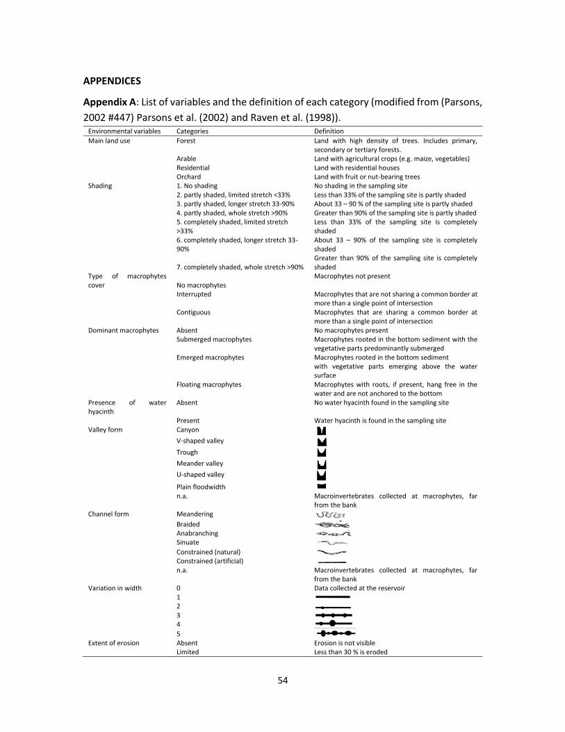
54

APPENDICES

Appendix A: List of variables and the definition of each category (modified from (Parsons,

2002 #447) Parsons et al. (2002) and Raven et al. (1998)). Environmental variables Categories Definition

Main land use Forest Land with high density of trees. Includes primary, secondary or tertiary forests.

Arable Land with agricultural crops (e.g. maize, vegetables) Residential Land with residential houses Orchard Land with fruit or nut-bearing trees

Shading 1. No shading No shading in the sampling site 2. partly shaded, limited stretch <33% Less than 33% of the sampling site is partly shaded 3. partly shaded, longer stretch 33-90% About 33 – 90 % of the sampling site is partly shaded 4. partly shaded, whole stretch >90% Greater than 90% of the sampling site is partly shaded 5. completely shaded, limited stretch

>33% Less than 33% of the sampling site is completely shaded

6. completely shaded, longer stretch 33-90%

About 33 – 90% of the sampling site is completely shaded

7. completely shaded, whole stretch >90%

Greater than 90% of the sampling site is completely shaded

Type of macrophytes cover No macrophytes

Macrophytes not present

Interrupted Macrophytes that are not sharing a common border at more than a single point of intersection

Contiguous Macrophytes that are sharing a common border at more than a single point of intersection

Dominant macrophytes Absent No macrophytes present Submerged macrophytes Macrophytes rooted in the bottom sediment with the

vegetative parts predominantly submerged Emerged macrophytes Macrophytes rooted in the bottom sediment

with vegetative parts emerging above the water surface

Floating macrophytes Macrophytes with roots, if present, hang free in the water and are not anchored to the bottom

Presence of water hyacinth

Absent No water hyacinth found in the sampling site

Present Water hyacinth is found in the sampling site Valley form Canyon

V-shaped valley

Trough

Meander valley

U-shaped valley

Plain floodwidth n.a. Macroinvertebrates collected at macrophytes, far

from the bank Channel form Meandering Braided Anabranching Sinuate Constrained (natural) Constrained (artificial) n.a. Macroinvertebrates collected at macrophytes, far

from the bank Variation in width 0 Data collected at the reservoir 1 2 3 4 5 Extent of erosion Absent Erosion is not visible Limited Less than 30 % is eroded

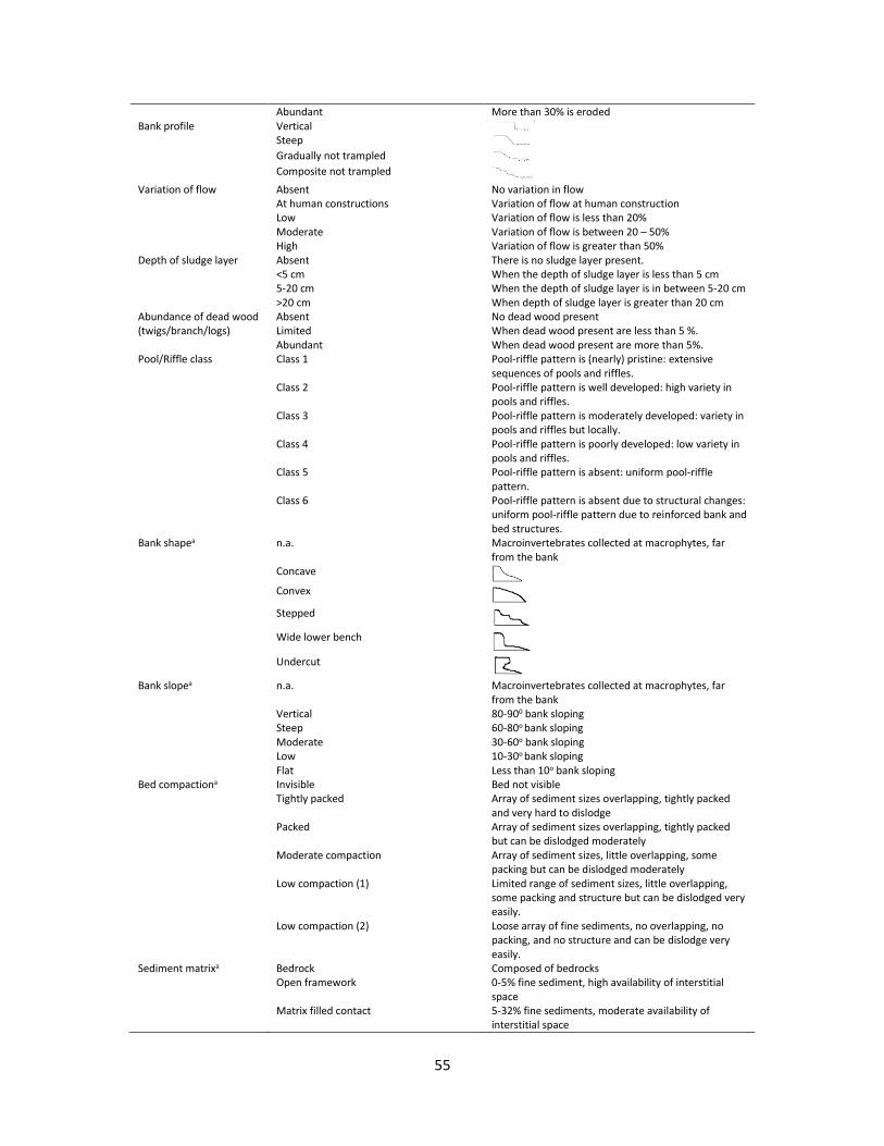
55

Abundant More than 30% is eroded Bank profile Vertical Steep Gradually not trampled Composite not trampled

Variation of flow Absent No variation in flow At human constructions Variation of flow at human construction Low Variation of flow is less than 20% Moderate Variation of flow is between 20 – 50% High Variation of flow is greater than 50% Depth of sludge layer Absent There is no sludge layer present. <5 cm When the depth of sludge layer is less than 5 cm 5-20 cm When the depth of sludge layer is in between 5-20 cm >20 cm When depth of sludge layer is greater than 20 cm Abundance of dead wood Absent No dead wood present (twigs/branch/logs) Limited When dead wood present are less than 5 %. Abundant When dead wood present are more than 5%. Pool/Riffle class Class 1 Pool-riffle pattern is (nearly) pristine: extensive

sequences of pools and riffles. Class 2 Pool-riffle pattern is well developed: high variety in

pools and riffles. Class 3 Pool-riffle pattern is moderately developed: variety in

pools and riffles but locally. Class 4 Pool-riffle pattern is poorly developed: low variety in

pools and riffles. Class 5 Pool-riffle pattern is absent: uniform pool-riffle

pattern. Class 6 Pool-riffle pattern is absent due to structural changes:

uniform pool-riffle pattern due to reinforced bank and bed structures.

Bank shapea n.a. Macroinvertebrates collected at macrophytes, far from the bank

Concave

Convex

Stepped

Wide lower bench

Undercut

Bank slopea n.a. Macroinvertebrates collected at macrophytes, far from the bank

Vertical 80-900 bank sloping Steep 60-80o bank sloping Moderate 30-60o bank sloping Low 10-30o bank sloping Flat Less than 10o bank sloping Bed compactiona Invisible Bed not visible Tightly packed Array of sediment sizes overlapping, tightly packed

and very hard to dislodge Packed Array of sediment sizes overlapping, tightly packed

but can be dislodged moderately Moderate compaction Array of sediment sizes, little overlapping, some

packing but can be dislodged moderately Low compaction (1) Limited range of sediment sizes, little overlapping,

some packing and structure but can be dislodged very easily.

Low compaction (2) Loose array of fine sediments, no overlapping, no packing, and no structure and can be dislodge very easily.

Sediment matrixa Bedrock Composed of bedrocks Open framework 0-5% fine sediment, high availability of interstitial

space Matrix filled contact 5-32% fine sediments, moderate availability of

interstitial space

56

Framework dilated 32-60% fine sediments, low availability of interstitial space

Matrix dominated Greater than 60% fine sediments, interstitial space virtually absent

Sediment angularitya Very angular

Angular

Sub-angular Rounded

Well rounded

Cobble, pebbles and gravel fractions not

present

Main sediment type Coarse Consists of boulder, cobble, pebbles, sand (except fine sand)

Fines Consists of fine sand, silt, clay

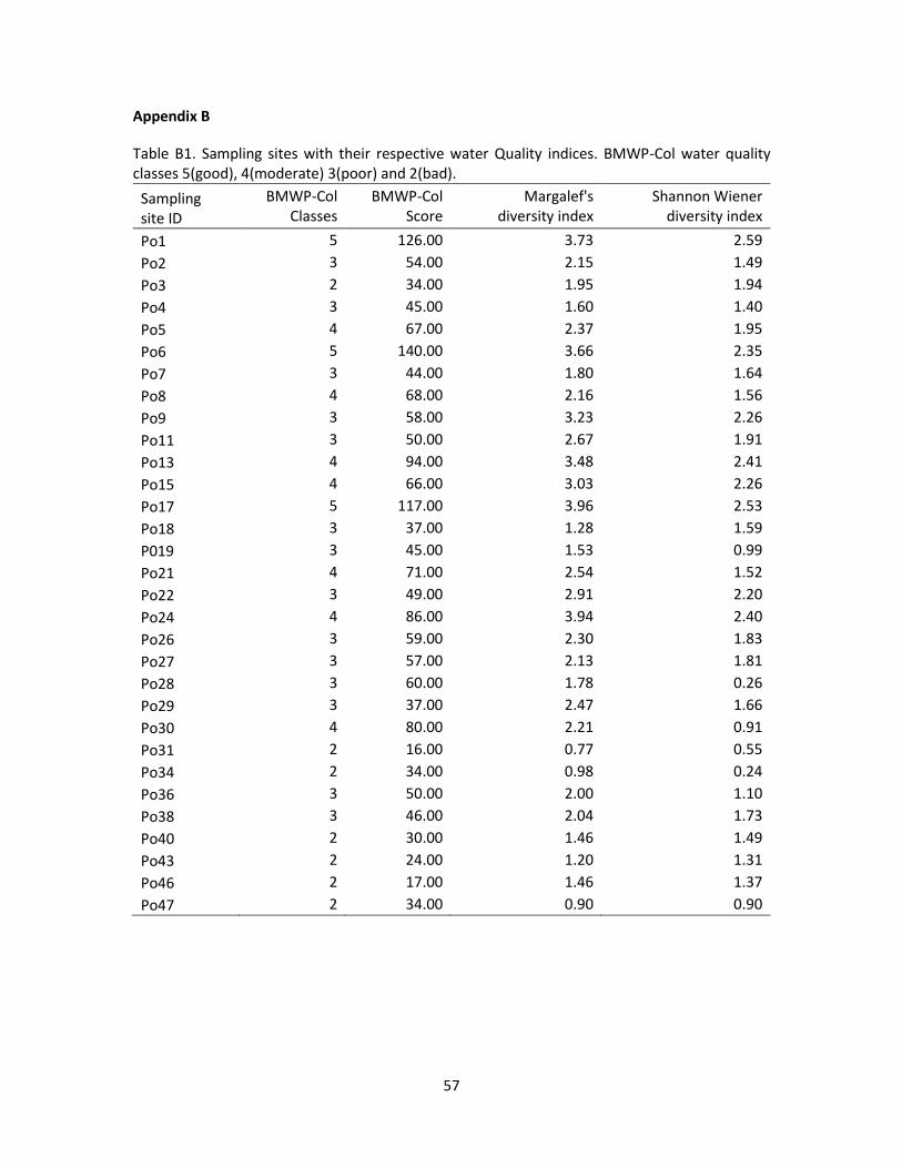
57

Appendix B

Table B1. Sampling sites with their respective water Quality indices. BMWP-Col water quality classes 5(good), 4(moderate) 3(poor) and 2(bad).

Sampling site ID

BMWP-Col Classes

BMWP-Col Score

Margalef's diversity index

Shannon Wiener diversity index

Po1 5 126.00 3.73 2.59

Po2 3 54.00 2.15 1.49

Po3 2 34.00 1.95 1.94

Po4 3 45.00 1.60 1.40

Po5 4 67.00 2.37 1.95

Po6 5 140.00 3.66 2.35

Po7 3 44.00 1.80 1.64

Po8 4 68.00 2.16 1.56

Po9 3 58.00 3.23 2.26

Po11 3 50.00 2.67 1.91

Po13 4 94.00 3.48 2.41

Po15 4 66.00 3.03 2.26

Po17 5 117.00 3.96 2.53

Po18 3 37.00 1.28 1.59

P019 3 45.00 1.53 0.99

Po21 4 71.00 2.54 1.52

Po22 3 49.00 2.91 2.20

Po24 4 86.00 3.94 2.40

Po26 3 59.00 2.30 1.83

Po27 3 57.00 2.13 1.81

Po28 3 60.00 1.78 0.26

Po29 3 37.00 2.47 1.66

Po30 4 80.00 2.21 0.91

Po31 2 16.00 0.77 0.55

Po34 2 34.00 0.98 0.24

Po36 3 50.00 2.00 1.10

Po38 3 46.00 2.04 1.73

Po40 2 30.00 1.46 1.49

Po43 2 24.00 1.20 1.31

Po46 2 17.00 1.46 1.37

Po47 2 34.00 0.90 0.90

58

Table B2: Physicochemical variables

Sampling site ID

Velocity Temp. Cond. pH DO DO-Sat Chlor. a Turbidity

COD BOD5

Nitrate-N

Nitrite-N

NH4-N

Total-N PO3

−4-P Total-

P TOC

BMWP-Col

(scores) (m/s) (°C) (µS/cm) (-) (mg/L

) (%) (µg/L) (mg/L) (mg/L)

(mg/L) (mg/L) (mg/L)

(mg/L) (mg/L) (mg/L)

(mg/L) (mg/L)

Po1 126 0.56 26.16 294.00 8.26 8.72 108.34 2.97 0.00 *3 2.34 *0.230 0.0020 0.126 0.70 0.122 0.119 *3.00

Po2 54 0.07 26.66 270.00 8.34 8.34 104.46 1.88 0.26 *3 3.54 *0.230 0.0020 0.067 *0.5 0.126 0.111 *3.00

Po3 34 0.00 27.47 253.00 6.50 2.22 28.29 4.25 0.64 4 5.86 0.243 *0.0015 0.054 0.80 0.050 *0.05

0 4.36

Po4 45 0.00 29.93 196.87 8.10 9.25 122.76 9.39 2.97 9 4.41 *0.230 0.0020 0.057 0.60 *0.050 0.062 5.24

Po5 67 0.35 26.67 316.40 8.17 8.30 104.11 2.41 0.00 *3 5.45 *0.230 0.0020 0.063 1.10 0.119 0.120 *3.00

Po6 140 0.56 25.83 878.47 7.92 7.94 98.16 4.71 2.79 *3 3.04 0.508 0.0050 0.044 0.80 0.238 0.156 3.01

Po7 44 0.10 26.33 425.00 8.09 7.94 98.99 1.86 0.01 *3 5.58 *0.230 0.0020 0.08 0.80 0.157 0.211 *3.00

Po8 68 0.00 31.33 195.00 8.81 11.84 160.96 16.61 3.15 7 4.72 *0.230 0.0030 0.04 1.60 0.051 0.096 5.81

Po9 58 0.00 26.48 164.47 7.14 7.71 96.30 6.61 23.77 4 4.33 0.265 0.0230 0.136 0.90 0.195 0.237 3.68

Po11 50 0.54 26.70 169.00 7.38 7.19 90.19 7.17 34.54 *3 3.89 0.285 0.0320 0.079 *0.5 0.198 0.201 3.22

Po13 94 0.88 25.69 176.00 7.54 7.42 91.37 5.64 25.24 *3 4.18 0.346 0.0340 0.141 *0.5 0.187 0.201 10.30

Po15 66 0.81 25.56 198.00 7.64 7.36 90.37 5.77 26.71 *3 1.95 0.590 0.0300 0.044 *0.5 0.192 0.209 14.00

Po17 117 0.69 25.89 239.00 7.77 7.48 92.46 6.01 28.85 *3 0.90 0.525 0.0210 0.098 1.30 0.211 0.233 13.40

Po18 37 0.00 27.21 310.00 8.35 9.74 123.25 8.01 27.15 *3 2.10 0.481 0.0170 0.101 1.20 0.247 0.267 17.00

Po19 45 0.54 26.38 310.33 7.91 8.14 101.53 7.26 28.35 *3 0.79 0.549 0.0170 0.055 0.60 0.237 0.254 16.30

Po21 71 0.44 28.01 343.00 7.82 7.74 99.34 5.73 28.60 *3 1.10 0.531 0.0220 0.185 0.80 0.262 0.243 16.70

Po22 49 0.54 27.82 345.00 7.81 7.66 98.07 6.57 30.37 *3 3.91 0.528 0.0220 0.096 1.20 0.235 0.204 18.90

Po24 86 0.63 28.55 981.73 7.83 7.57 98.31 11.61 26.71 5 2.59 0.616 0.0260 0.069 2.90 0.242 0.274 29.20

Po26 59 0.87 28.31 1751.00 7.82 7.64 99.07 9.68 16.55 5 1.10 1.250 0.0470 0.087 1.40 0.243 0.204 22.30

Po27 57 0.72 28.55 1503.73 7.94 8.00 104.10 8.47 14.22 11 1.30 1.810 0.0440 0.134 2.20 0.186 0.132 27.90

Po28 60 0.45 28.38 1547.87 7.96 7.79 100.98 7.01 10.57 4 1.10 1.900 0.0480 0.123 5.70 0.109 0.117 20.60

Po29 37 0.39 28.52 1560.87 7.83 6.79 88.27 7.99 18.42 8 1.23 2.360 0.0490 0.152 2.40 0.190 0.209 19.10

Po30 80 0.20 28.42 1449.00 7.87 6.66 86.43 5.94 16.35 *3 2.47 2.810 0.0300 0.099 5.40 0.255 0.286 19.80

Po31 16 0.19 28.35 1418.27 7.99 6.73 87.12 40.89 18.54 *3 4.40 2.210 0.0340 0.061 4.20 0.217 0.435 31.10

Po34 34 0.54 28.73 1499.73 7.70 6.79 88.61 32.05 9.87 *3 2.76 2.540 0.1010 0.055 2.60 0.303 0.446 23.60

Po36 50 0.60 28.56 1575.00 7.66 5.89 76.63 19.03 8.49 *3 3.50 2.650 0.1140 0.084 4.20 0.333 0.534 32.00

Po38 46 0.11 28.20 1749.00 7.83 7.79 100.75 43.59 9.51 *3 2.88 2.390 0.0980 0.095 2.50 0.238 0.354 25.30

Po40 30 0.07 29.19 1931.00 8.21 10.39 136.81 53.09 7.30 *3 3.77 1.610 0.1100 0.063 1.00 0.308 0.335 23.50

Po43 24 0.50 27.56 2447.00 7.74 6.15 78.86 7.51 7.45 14 2.38 1.470 0.0590 0.058 1.70 0.315 0.333 17.30

Po46 17 0.30 27.32 49383.5

3 7.97 5.73 87.07 6.71 32.94 142 2.33 0.310 0.0130 0.041 *0.5 0.144 0.236 22.40

Po47 34 0.00 29.76 1922.07 8.36 18.29 243.18 55.16 6.44 18 n/a 1.470 0.1430 0.035 3.80 0.200 0.295 37.70

*Values expressed as the detection limit of the kit

n/a = not available

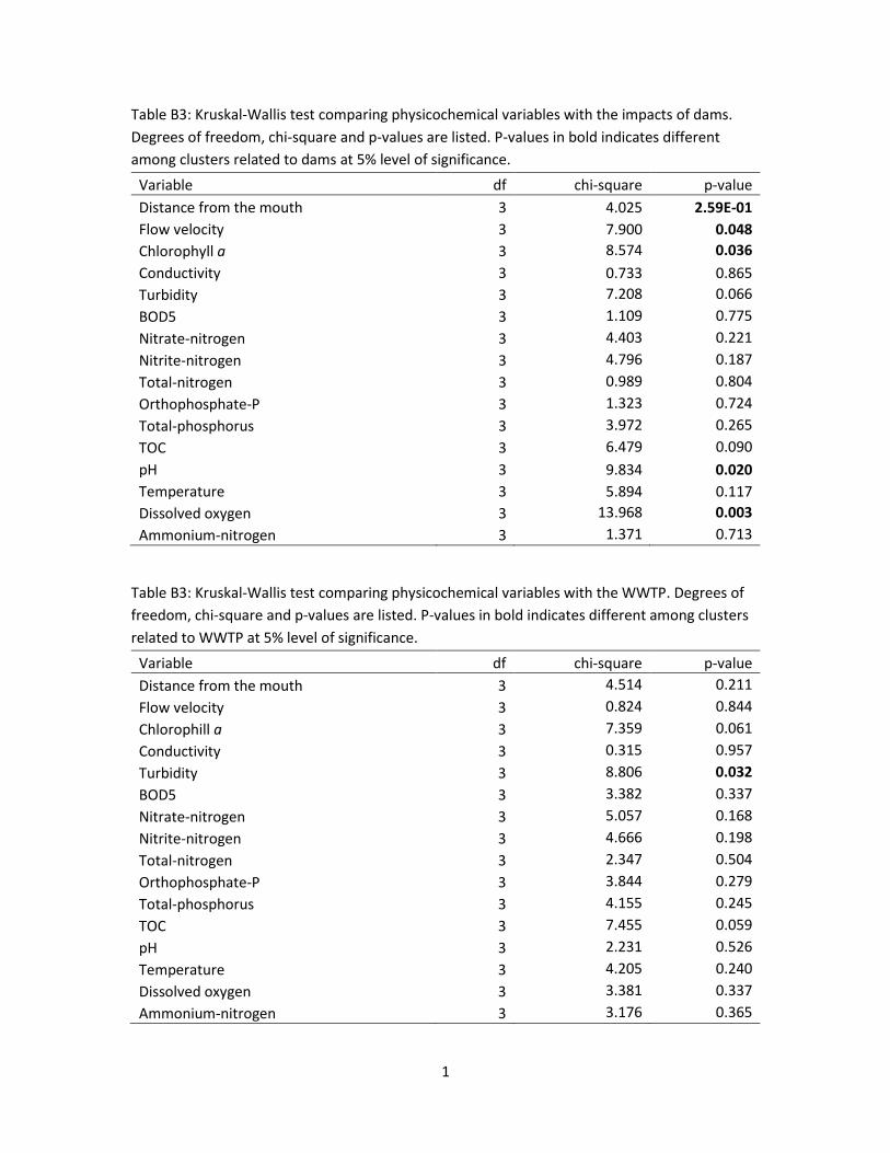
1

Table B3: Kruskal-Wallis test comparing physicochemical variables with the impacts of dams.

Degrees of freedom, chi-square and p-values are listed. P-values in bold indicates different

among clusters related to dams at 5% level of significance.

Variable df chi-square p-value

Distance from the mouth 3 4.025 2.59E-01

Flow velocity 3 7.900 0.048

Chlorophyll a 3 8.574 0.036

Conductivity 3 0.733 0.865

Turbidity 3 7.208 0.066

BOD5 3 1.109 0.775

Nitrate-nitrogen 3 4.403 0.221

Nitrite-nitrogen 3 4.796 0.187

Total-nitrogen 3 0.989 0.804

Orthophosphate-P 3 1.323 0.724

Total-phosphorus 3 3.972 0.265

TOC 3 6.479 0.090

pH 3 9.834 0.020

Temperature 3 5.894 0.117

Dissolved oxygen 3 13.968 0.003

Ammonium-nitrogen 3 1.371 0.713

Table B3: Kruskal-Wallis test comparing physicochemical variables with the WWTP. Degrees of

freedom, chi-square and p-values are listed. P-values in bold indicates different among clusters

related to WWTP at 5% level of significance.

Variable df chi-square p-value

Distance from the mouth 3 4.514 0.211

Flow velocity 3 0.824 0.844

Chlorophill a 3 7.359 0.061

Conductivity 3 0.315 0.957

Turbidity 3 8.806 0.032

BOD5 3 3.382 0.337

Nitrate-nitrogen 3 5.057 0.168

Nitrite-nitrogen 3 4.666 0.198

Total-nitrogen 3 2.347 0.504

Orthophosphate-P 3 3.844 0.279

Total-phosphorus 3 4.155 0.245

TOC 3 7.455 0.059

pH 3 2.231 0.526

Temperature 3 4.205 0.240

Dissolved oxygen 3 3.381 0.337

Ammonium-nitrogen 3 3.176 0.365

2

Appendix C

Figure C1: Boxplots of dominand land use, shading, main macrophyte, water hyacinth, valley

form and chanel form in relation with BMWP-Colombia scores.

Figure C2: Boxplots of variation in with, erosion, curvature of erosion, with of erosion, profile of

the banks and variation in flow in relation with BMWP-Colombia scores.

3

Figure C3: Boxplots of sludge layer, twigs, branches, logs, dominant mineral substrates and

dominant bank material in relation with BMWP-Colombia scores

Figure C4: Boxplots of bank shapes, bank slopes, bed compaction, sediemt matrix, sediment

angularity and riffle classes in relation with BMWP-Colombia scores.

4

Figure C5: Boxplots of Dutch method, LISEC index, land use, dams and municipal wastewater

treatment plant (MWWTP) and type of water course in relation with BMWP-Colombia scores.

Figure C6: Physicochemical variables in relation with distance from the mouth.

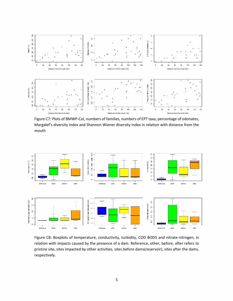
5

Figure C7: Plots of BMWP-Col, numbers of families, numbers of EPT taxa, percentage of odonates,

Margalef’s diversity index and Shannon Wiener diversity index in relation with distance from the

mouth

Figure C8: Boxplots of temperature, conductivity, turbidity, COD BOD5 and nitrate-nitrogen, in

relation with impacts caused by the presence of a dam. Reference, other, before, after refers to

pristine site, sites impacted by other activities, sites before dams(reservoir), sites after the dams,

respectively.

6

Figure C9: Boxplots of nitrite-nitrogen, ammonium-nitrogen, total-nitrogen, orthophosphate-

phosphorus, total-phosphorus and total organic carbon in relation with the impacts caused by

the presence of a dam. Reference, other, before, after refers to pristine site, sites impacted by

other activities, sites before dams(reservoir), sites after the dams, respectively.

Figure C10: Boxplots of BMWP-Col, number of families, numbers of EPT taxa, percentage of

odonates, Margalef’s diversity index and Shannon Wiener diversity index, in relation with the

impacts caused by the presence of a dam. Reference, other, before, after refers to pristine site,

sites impacted by other activities, sites before dams(reservoir), sites after the dams, respectively.

7

Figure C11: Boxplots of pH, dissolved oxygen, temperature and ammonium-nitrogen in relation

with land uses.

Figure C12: Boxplots of Dutch method and LISEC index in relation with land uses

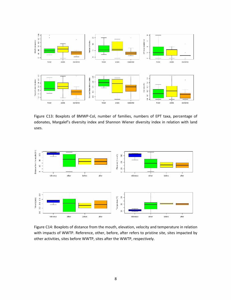
8

Figure C13: Boxplots of BMWP-Col, number of families, numbers of EPT taxa, percentage of

odonates, Margalef’s diversity index and Shannon Wiener diversity index in relation with land

uses.

Figure C14: Boxplots of distance from the mouth, elevation, velocity and temperature in relation

with impacts of WWTP. Reference, other, before, after refers to pristine site, sites impacted by

other activities, sites before WWTP, sites after the WWTP, respectively.

9

Figure C15: Boxplots of conductivity, pH, dissolved oxygen and chlorophyll in relation with impacts

of WWTP. Reference, other, before, after refers to pristine site, sites impacted by other activities,

sites before WWTP, sites after the WWTP, respectively.

Figure C16: Boxplots of nitrate-nitrogen, nitrite-nitrogen, ammonium-nitrogen and total-nitrogen

in relation with impacts of WWTP. Reference, other, before, after refers to pristine site, sites

impacted by other activities, sites before WWTP, sites after the WWTP, respectively.

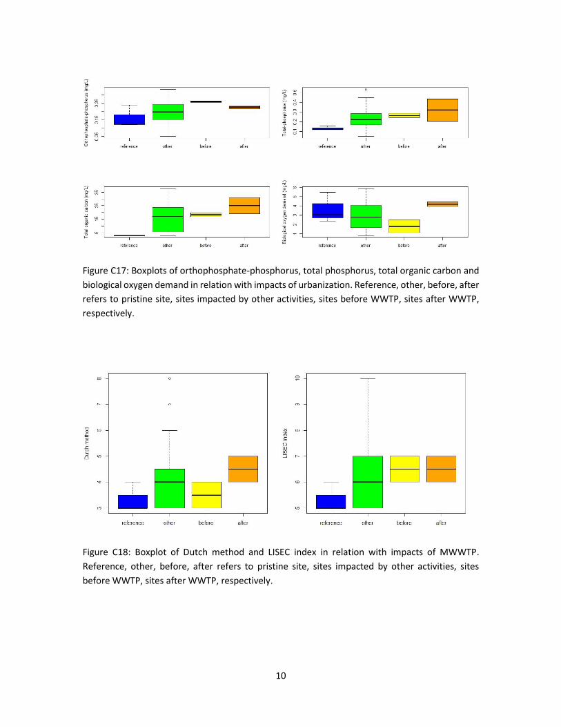
10

Figure C17: Boxplots of orthophosphate-phosphorus, total phosphorus, total organic carbon and

biological oxygen demand in relation with impacts of urbanization. Reference, other, before, after

refers to pristine site, sites impacted by other activities, sites before WWTP, sites after WWTP,

respectively.

Figure C18: Boxplot of Dutch method and LISEC index in relation with impacts of MWWTP.

Reference, other, before, after refers to pristine site, sites impacted by other activities, sites

before WWTP, sites after WWTP, respectively.

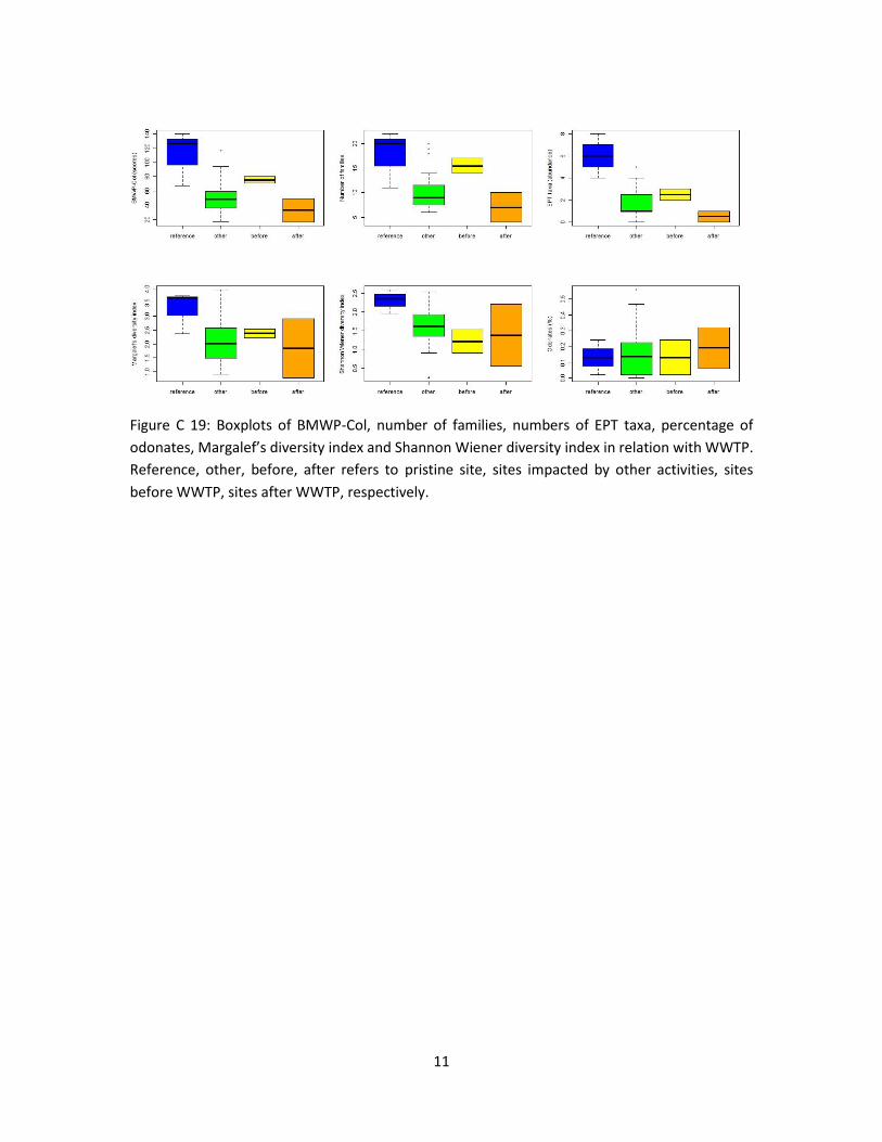
11

Figure C 19: Boxplots of BMWP-Col, number of families, numbers of EPT taxa, percentage of

odonates, Margalef’s diversity index and Shannon Wiener diversity index in relation with WWTP.

Reference, other, before, after refers to pristine site, sites impacted by other activities, sites

before WWTP, sites after WWTP, respectively.