UNSFLO: A Numerical Method For Unsteady Inviscid Flow In ...
SPC 307Aerodynamics
Lecture 6Inviscid (Potential) Flow
March 19, 2018
Sep. 18, 20161
2
3
4
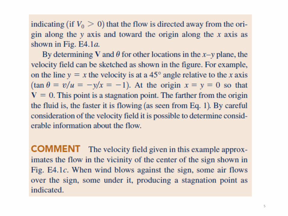
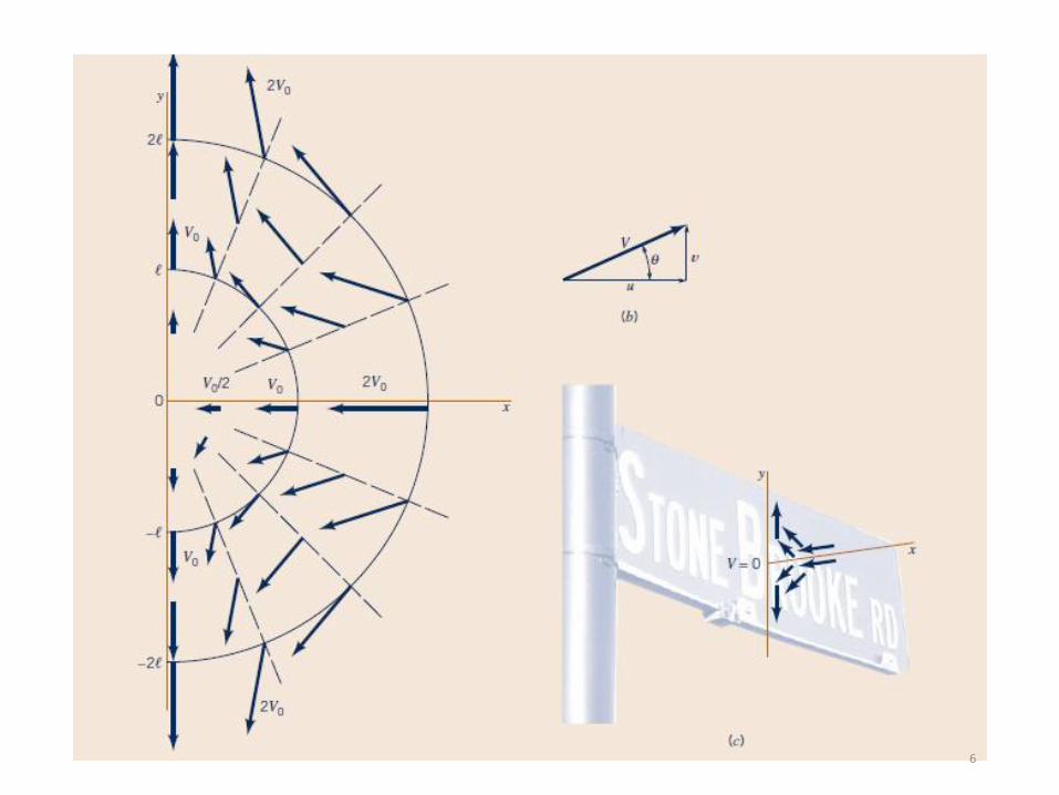
5
6
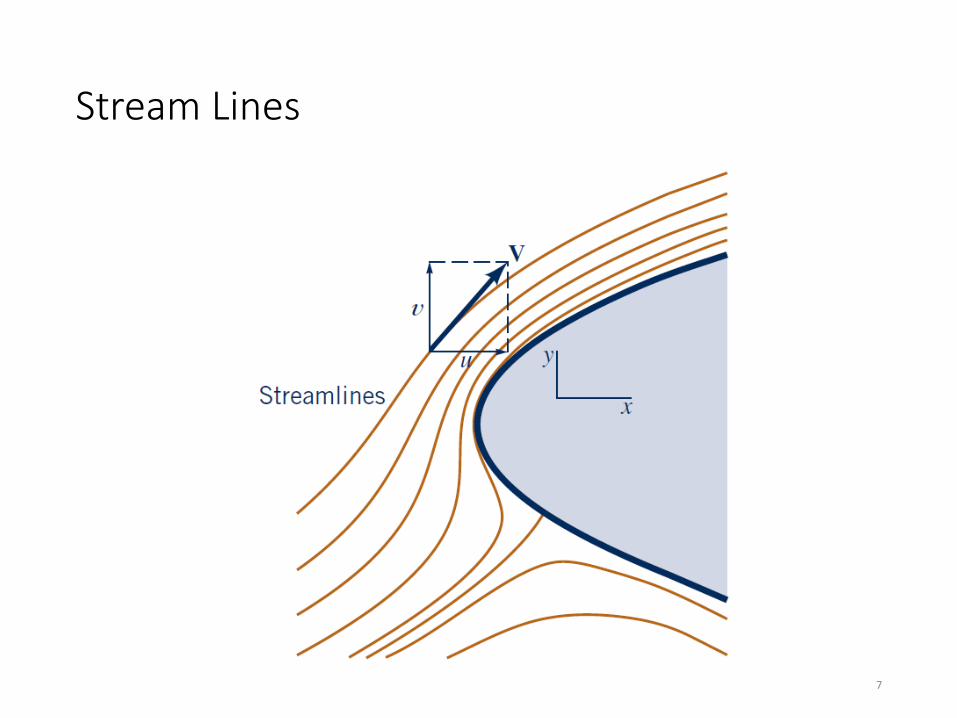
Stream Lines
7
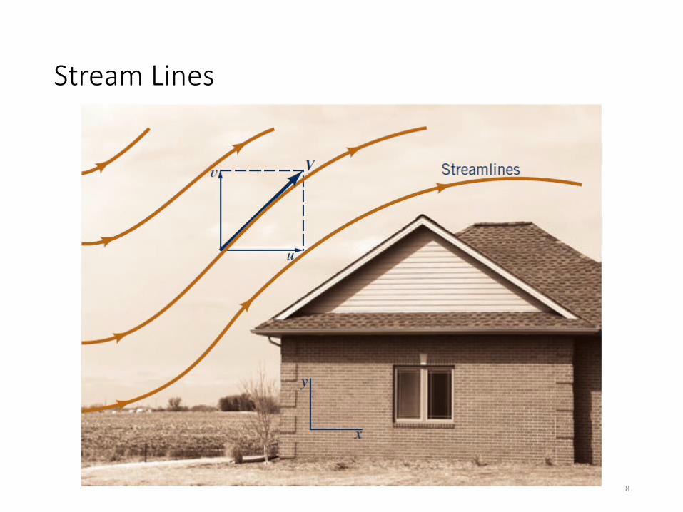
Stream Lines
8
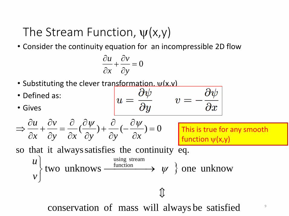
The Stream Function, (x,y)• Consider the continuity equation for an incompressible 2D flow
• Substituting the clever transformation, (x,y)
• Defined as:
• Gives
This is true for any smoothfunction (x,y)
satisfied be always willmass ofon conservati
unknow one unknows two functionstream using
v
ueq. continuity thesatisfies alwaysit that so
0)()(
xyyxy
v
x
u
0
y
v
x
u
9
10
11
12
13
14
15
16
17
The Stream Function, • Why do this?
• Single variable replaces (u,v).
• Once is known, (u,v) can be determined.
• Physical significance
1. Curves of constant are streamlines of the flow
2. Difference in between streamlines is equal to
volume flow rate between streamlines
18
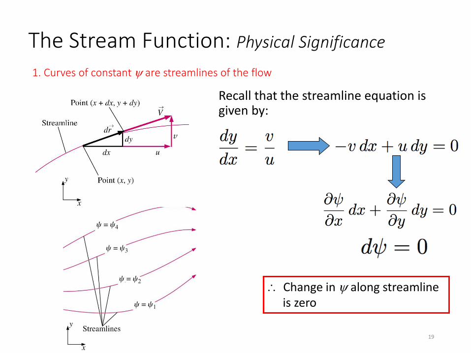
The Stream Function: Physical Significance
Recall that the streamline equation is given by:
Change in along streamline is zero
1. Curves of constant are streamlines of the flow
19
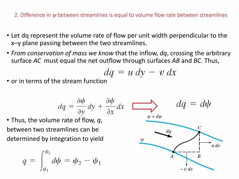
• Let dq represent the volume rate of flow per unit width perpendicular to the x–y plane passing between the two streamlines.
• From conservation of mass we know that the inflow, dq, crossing the arbitrary surface AC must equal the net outflow through surfaces AB and BC. Thus,
• or in terms of the stream function
• Thus, the volume rate of flow, q,
between two streamlines can be
determined by integration to yield
2. Difference in between streamlines is equal to volume flow rate between streamlines
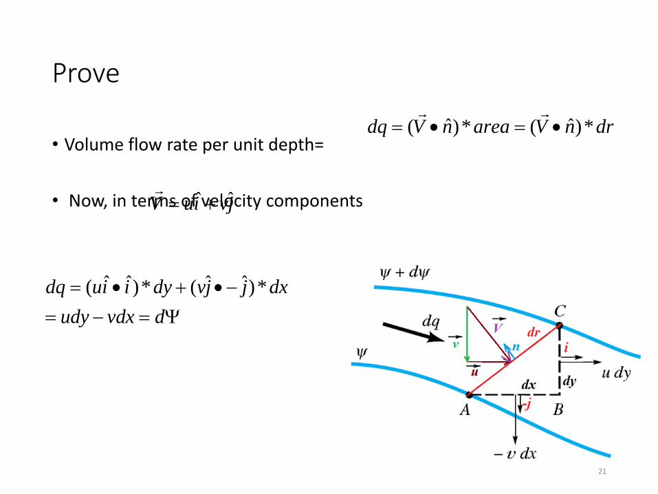
Prove
• Volume flow rate per unit depth=
• Now, in terms of velocity components
*)ˆ(*)ˆ( drnVareanVdq ••
jviuV ˆˆ
*)ˆˆ(*)ˆˆ(
••
dvdxudy
dxjjvdyiiudq
21
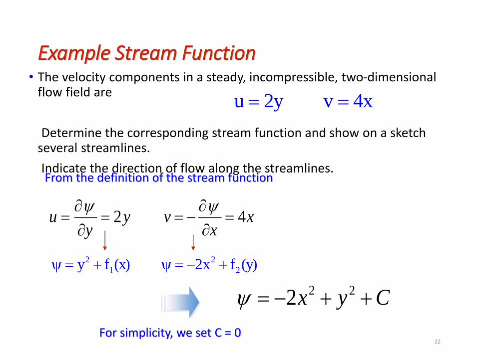
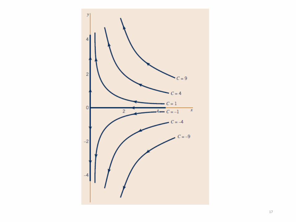
Example Stream Function• The velocity components in a steady, incompressible, two-dimensional
flow field are
Determine the corresponding stream function and show on a sketch several streamlines.
Indicate the direction of flow along the streamlines.
4xv2yu
(y)fx2(x)fy 2
2
1
2
From the definition of the stream function
xx
vyy
u 42
Cyx 222
For simplicity, we set C = 022
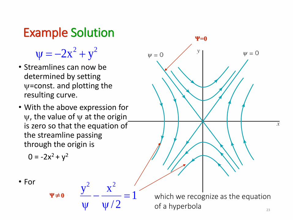
Example Solution
• Streamlines can now be determined by setting =const. and plotting the resulting curve.
• With the above expression for , the value of at the origin is zero so that the equation of the streamline passing through the origin is
0 = -2x2 + y2
• For
22 yx2
Ψ=0
Ψ≠0 12/
xy 22
which we recognize as the equation of a hyperbola
23
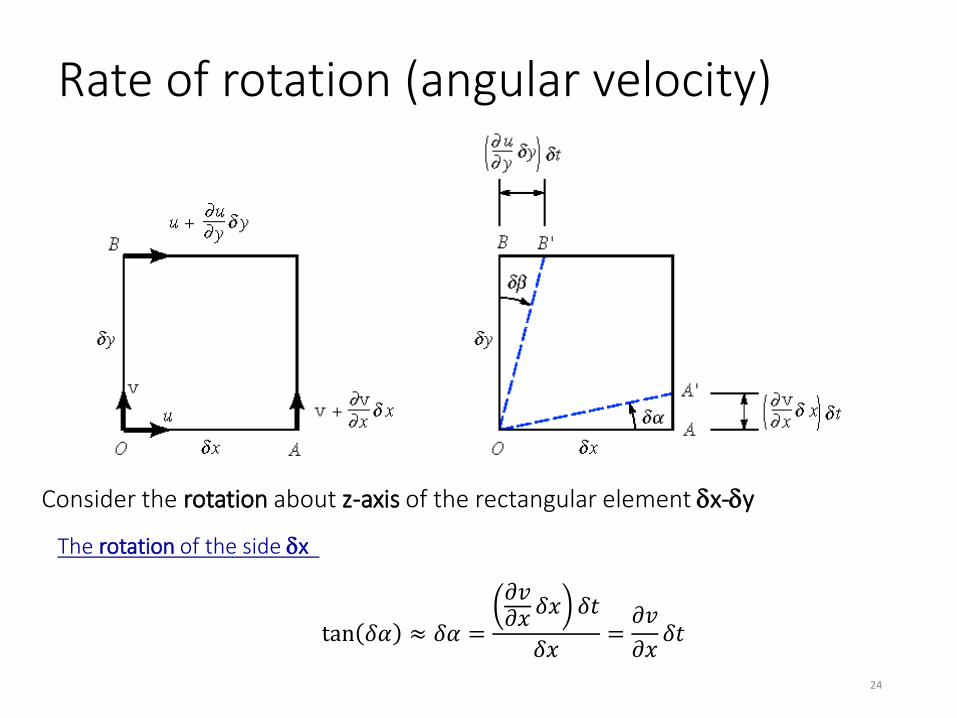
Rate of rotation (angular velocity)
tan 𝛿𝛼 ≈ 𝛿𝛼 =
𝜕𝑣𝜕𝑥
𝛿𝑥 𝛿𝑡
𝛿𝑥=𝜕𝑣
𝜕𝑥𝛿𝑡
Consider the rotation about z-axis of the rectangular element x-y
The rotation of the side x
24
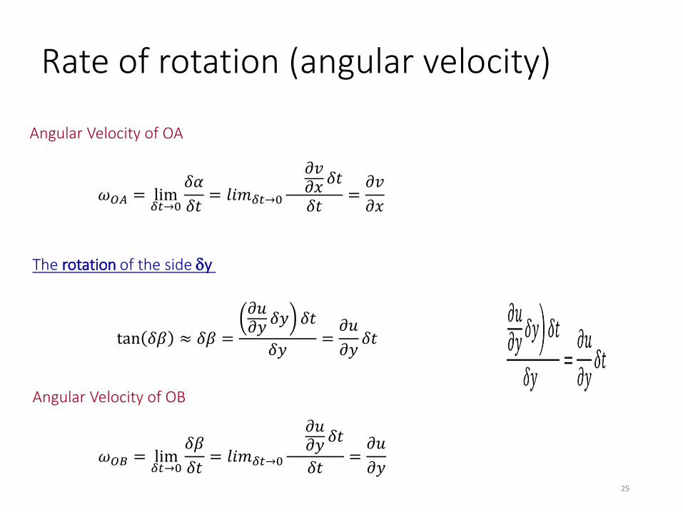
Rate of rotation (angular velocity)
Angular Velocity of OA
𝜔𝑂𝐴 = lim𝛿𝑡→0
𝛿𝛼
𝛿𝑡= 𝑙𝑖𝑚𝛿𝑡→0
𝜕𝑣𝜕𝑥
𝛿𝑡
𝛿𝑡=𝜕𝑣
𝜕𝑥
The rotation of the side y
𝜔𝑂𝐵 = lim𝛿𝑡→0
𝛿𝛽
𝛿𝑡= 𝑙𝑖𝑚𝛿𝑡→0
𝜕𝑢𝜕𝑦
𝛿𝑡
𝛿𝑡=𝜕𝑢
𝜕𝑦
Angular Velocity of OB
tan 𝛿𝛽 ≈ 𝛿𝛽 =
𝜕𝑢𝜕𝑦
𝛿𝑦 𝛿𝑡
𝛿𝑦=𝜕𝑢
𝜕𝑦𝛿𝑡
25
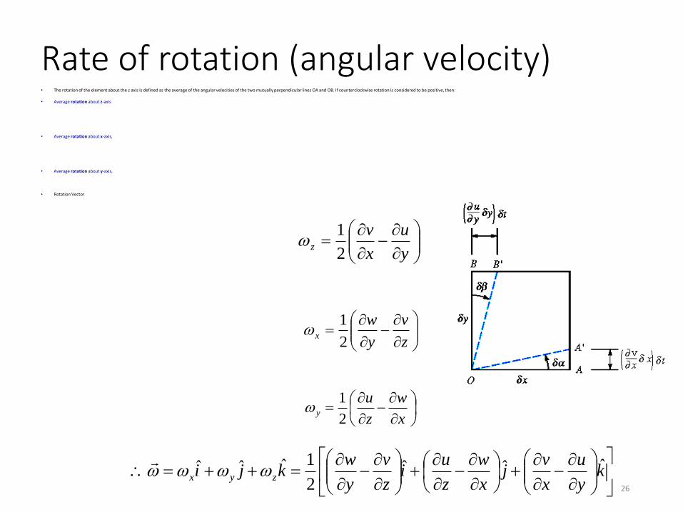
Rate of rotation (angular velocity)• The rotation of the element about the z axis is defined as the average of the angular velocities of the two mutually perpendicular lines OA and OB. If counterclockwise rotation is considered to be positive, then:
• Average rotation about z-axis
• Average rotation about x-axis,
• Average rotation about y-axis,
• Rotation Vector
y
u
x
vz
2
1
z
v
y
wx
2
1
x
w
z
uy
2
1
k
y
u
x
vj
x
w
z
ui
z
v
y
wkji zyx
ˆˆˆ2
1ˆˆˆ
26
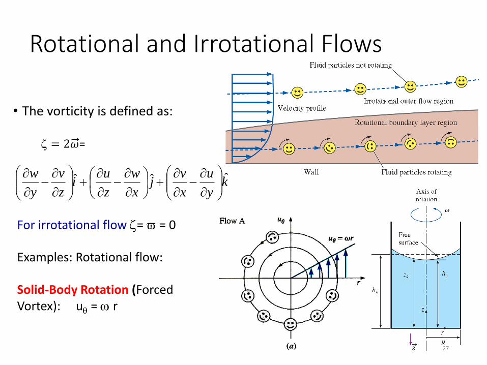
Rotational and Irrotational Flows
• The vorticity is defined as:
= 2𝜔=
ky
u
x
vj
x
w
z
ui
z
v
y
w ˆˆˆ
For irrotational flow = = 0
Examples: Rotational flow:
Solid-Body Rotation (Forced Vortex): u = r
27
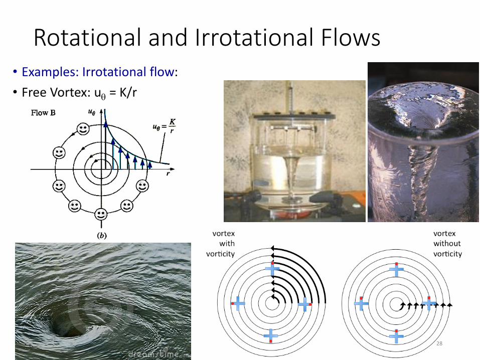
Rotational and Irrotational Flows• Examples: Irrotational flow:
• Free Vortex: u = K/r
28
29
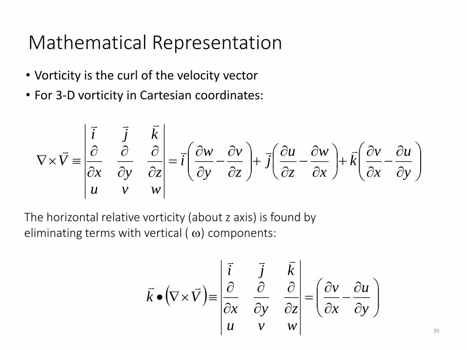
Mathematical Representation
• Vorticity is the curl of the velocity vector
• For 3-D vorticity in Cartesian coordinates:
y
u
x
vk
x
w
z
uj
z
v
y
wi
wvu
zyx
kji
V
The horizontal relative vorticity (about z axis) is found byeliminating terms with vertical () components:
•
y
u
x
v
wvu
zyx
kji
Vk
30
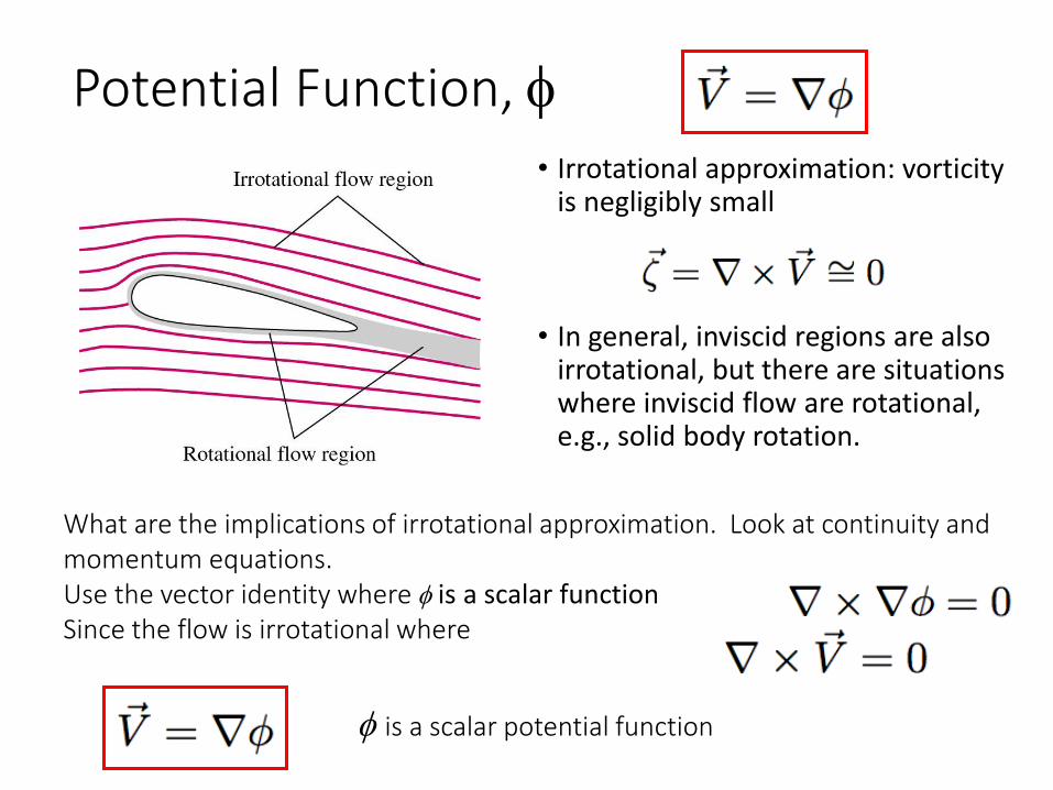
Potential Function, • Irrotational approximation: vorticity
is negligibly small
• In general, inviscid regions are also irrotational, but there are situations where inviscid flow are rotational, e.g., solid body rotation.
What are the implications of irrotational approximation. Look at continuity and momentum equations.Use the vector identity where is a scalar functionSince the flow is irrotational where
is a scalar potential function
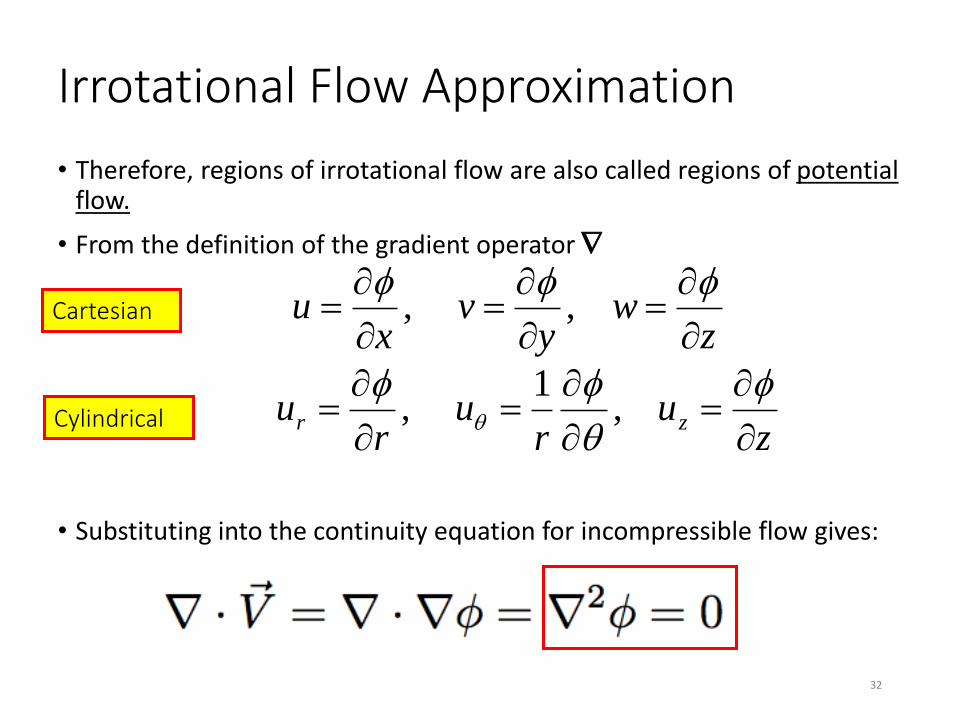
Irrotational Flow Approximation
• Therefore, regions of irrotational flow are also called regions of potential flow.
• From the definition of the gradient operator
• Substituting into the continuity equation for incompressible flow gives:
Cartesian
Cylindrical
zw
yv
xu
, ,
zu
ru
ru zr
,
1 ,
32
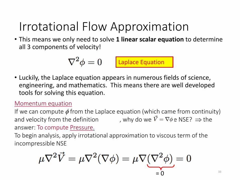
Irrotational Flow Approximation• This means we only need to solve 1 linear scalar equation to determine
all 3 components of velocity!
• Luckily, the Laplace equation appears in numerous fields of science, engineering, and mathematics. This means there are well developed tools for solving this equation.
Laplace Equation
Momentum equationIf we can compute from the Laplace equation (which came from continuity) and velocity from the definition , why do we need the NSE? the answer: To compute Pressure.To begin analysis, apply irrotational approximation to viscous term of the incompressible NSE
= 0 33
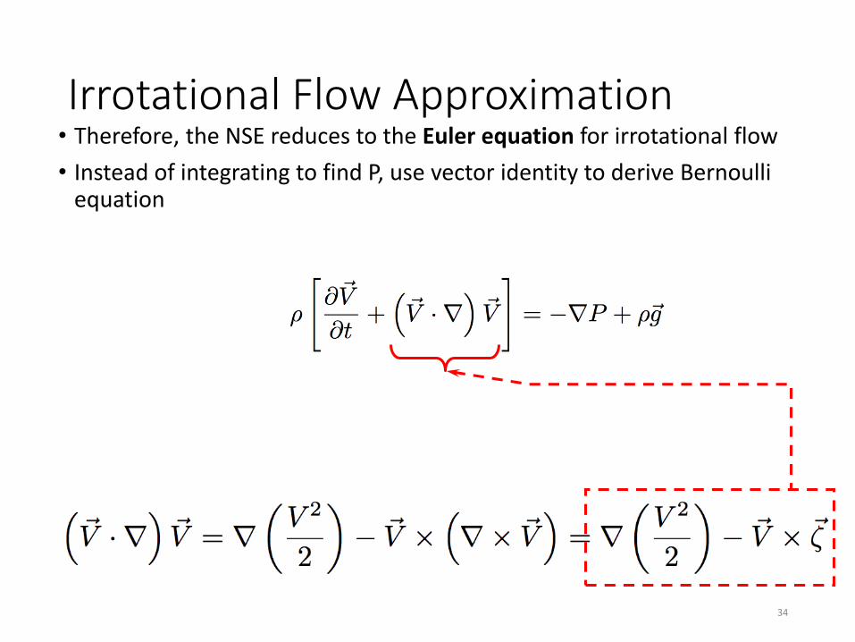
Irrotational Flow Approximation• Therefore, the NSE reduces to the Euler equation for irrotational flow
• Instead of integrating to find P, use vector identity to derive Bernoulli equation
34
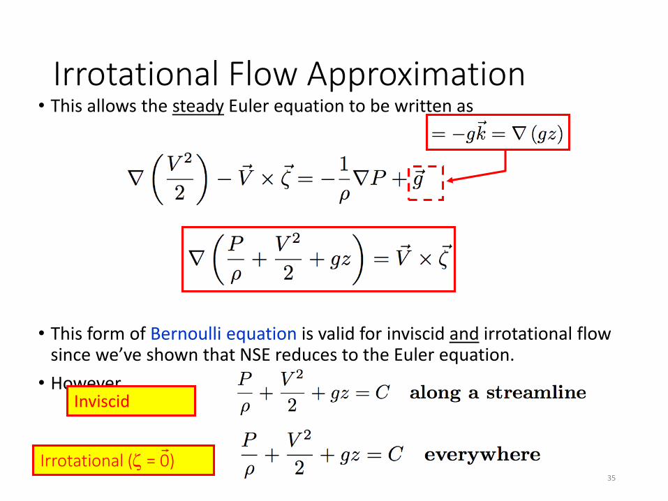
Irrotational Flow Approximation• This allows the steady Euler equation to be written as
• This form of Bernoulli equation is valid for inviscid and irrotational flow since we’ve shown that NSE reduces to the Euler equation.
• However, Inviscid
Irrotational ( = 0)35
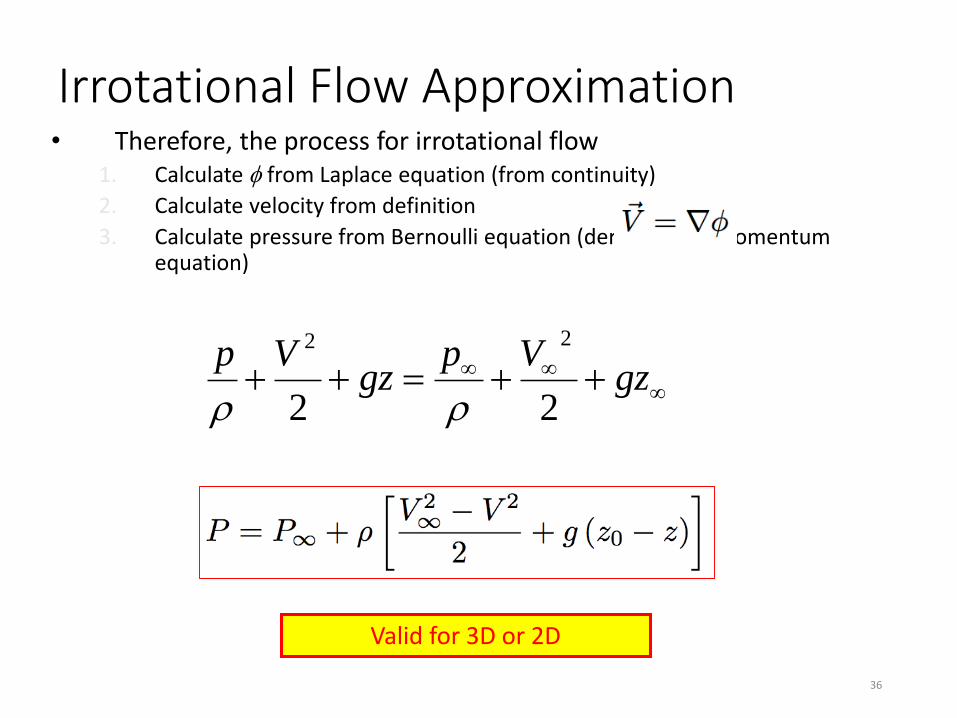
Irrotational Flow Approximation• Therefore, the process for irrotational flow
1. Calculate from Laplace equation (from continuity)
2. Calculate velocity from definition
3. Calculate pressure from Bernoulli equation (derived from momentum equation)
Valid for 3D or 2D
gz
Vpgz
Vp
22
22
36
Irrotational Flow Approximation2D Flows
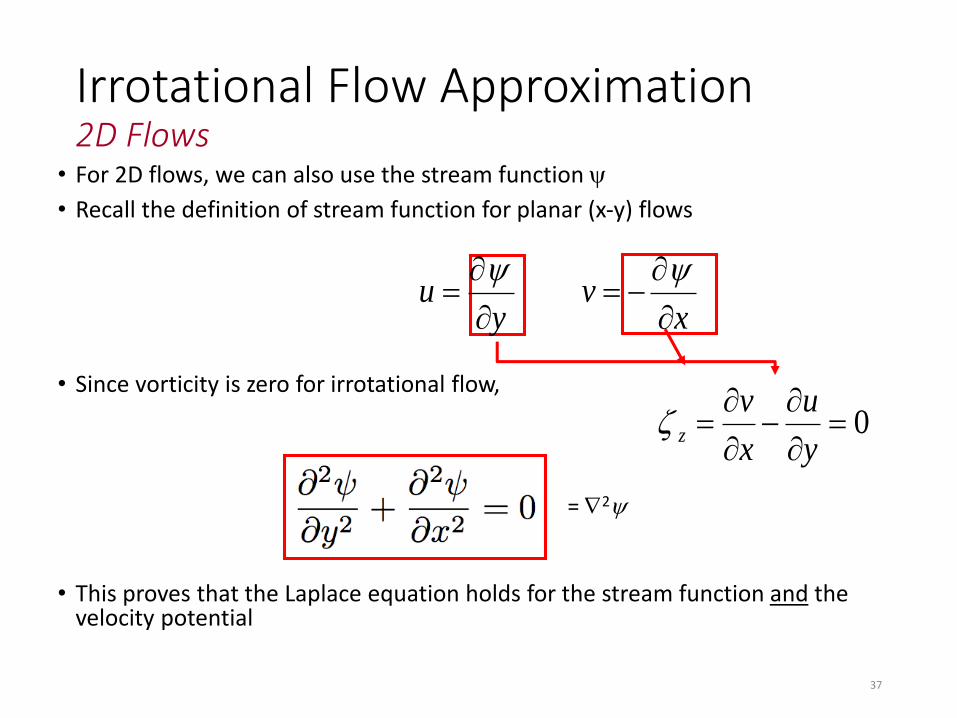
• For 2D flows, we can also use the stream function
• Recall the definition of stream function for planar (x-y) flows
• Since vorticity is zero for irrotational flow,
• This proves that the Laplace equation holds for the stream function and the velocity potential
xv
yu
0
y
u
x
vz
= 2
37
Irrotational Flow Approximation2D Flows
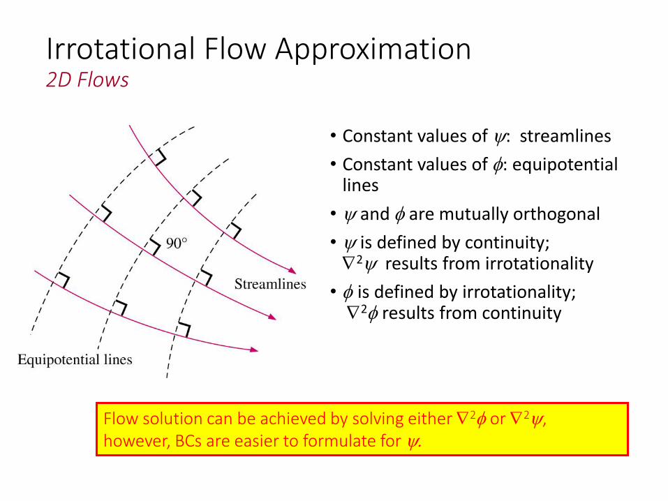
• Constant values of : streamlines
• Constant values of : equipotential lines
• and are mutually orthogonal
• is defined by continuity; 2 results from irrotationality
• is defined by irrotationality;2 results from continuity
Flow solution can be achieved by solving either 2 or 2, however, BCs are easier to formulate for
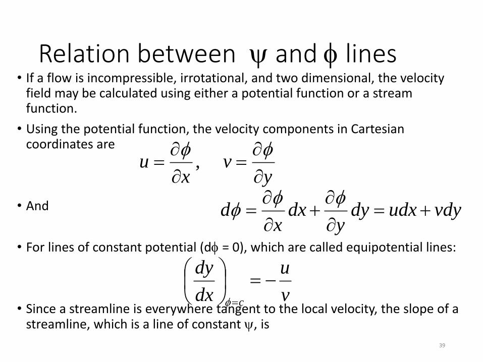
Relation between and lines• If a flow is incompressible, irrotational, and two dimensional, the velocity
field may be calculated using either a potential function or a stream function.
• Using the potential function, the velocity components in Cartesian coordinates are
• And
• For lines of constant potential (d = 0), which are called equipotential lines:
• Since a streamline is everywhere tangent to the local velocity, the slope of a streamline, which is a line of constant , is
yv
xu
,
vdyudxdyy
dxx
d
v
u
dx
dy
c
39
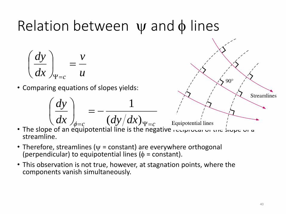
Relation between and lines
• Comparing equations of slopes yields:
• The slope of an equipotential line is the negative reciprocal of the slope of a streamline.
• Therefore, streamlines ( = constant) are everywhere orthogonal (perpendicular) to equipotential lines ( = constant).
• This observation is not true, however, at stagnation points, where the components vanish simultaneously.
u
v
dx
dy
c
cc dxdydx
dy
)(
1
40
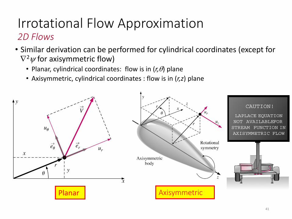
Irrotational Flow Approximation2D Flows• Similar derivation can be performed for cylindrical coordinates (except for 2 for axisymmetric flow)• Planar, cylindrical coordinates: flow is in (r,) plane
• Axisymmetric, cylindrical coordinates : flow is in (r,z) plane
Planar Axisymmetric
41
Irrotational Flow Approximation2D Flows
42
Potential flows Visualization
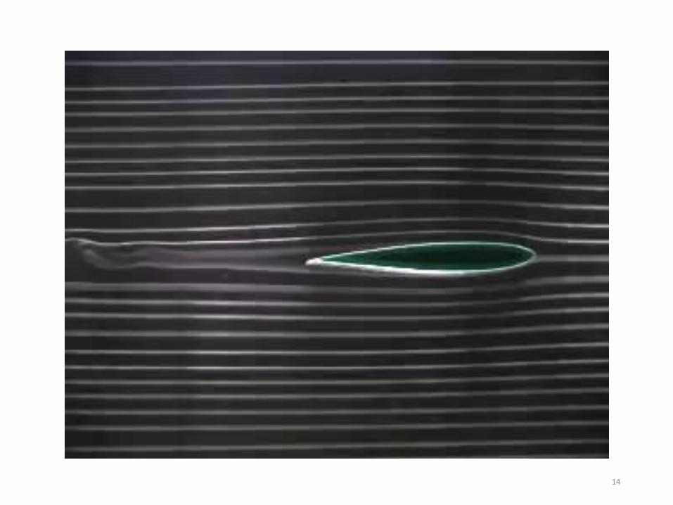
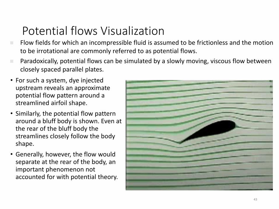
• For such a system, dye injected upstream reveals an approximate potential flow pattern around a streamlined airfoil shape.
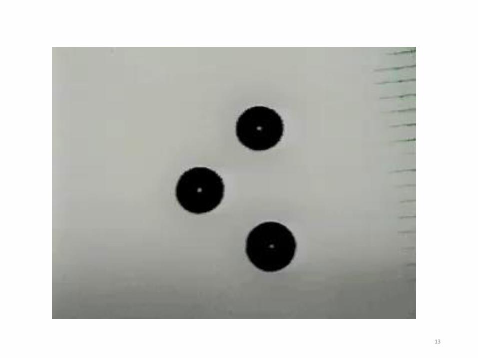
• Similarly, the potential flow pattern around a bluff body is shown. Even at the rear of the bluff body the streamlines closely follow the body shape.
• Generally, however, the flow would separate at the rear of the body, an important phenomenon not accounted for with potential theory.
Flow fields for which an incompressible fluid is assumed to be frictionless and the motion to be irrotational are commonly referred to as potential flows.
Paradoxically, potential flows can be simulated by a slowly moving, viscous flow between closely spaced parallel plates.
43
Irrotational Flow Approximation2D Flows
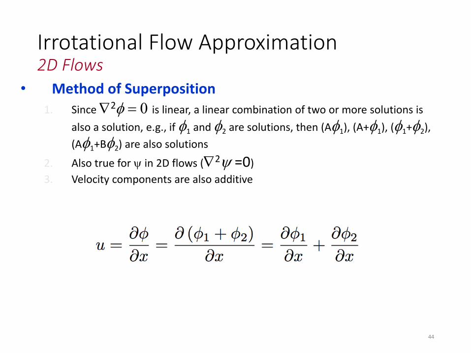
• Method of Superposition
1. Since 2 is linear, a linear combination of two or more solutions is
also a solution, e.g., if 1 and 2 are solutions, then (A1), (A+1), (1+2),
(A1+B2) are also solutions
2. Also true for in 2D flows (2 =0)
3. Velocity components are also additive
44
Irrotational Flow Approximation2D Flows
• Given the principal of superposition, there are several elementary planar irrotational flows which can be combined to create more complex flows.
• Elementary Planar Irrotational Flows• Uniform stream• Line source/sink• Line vortex• Doublet
45
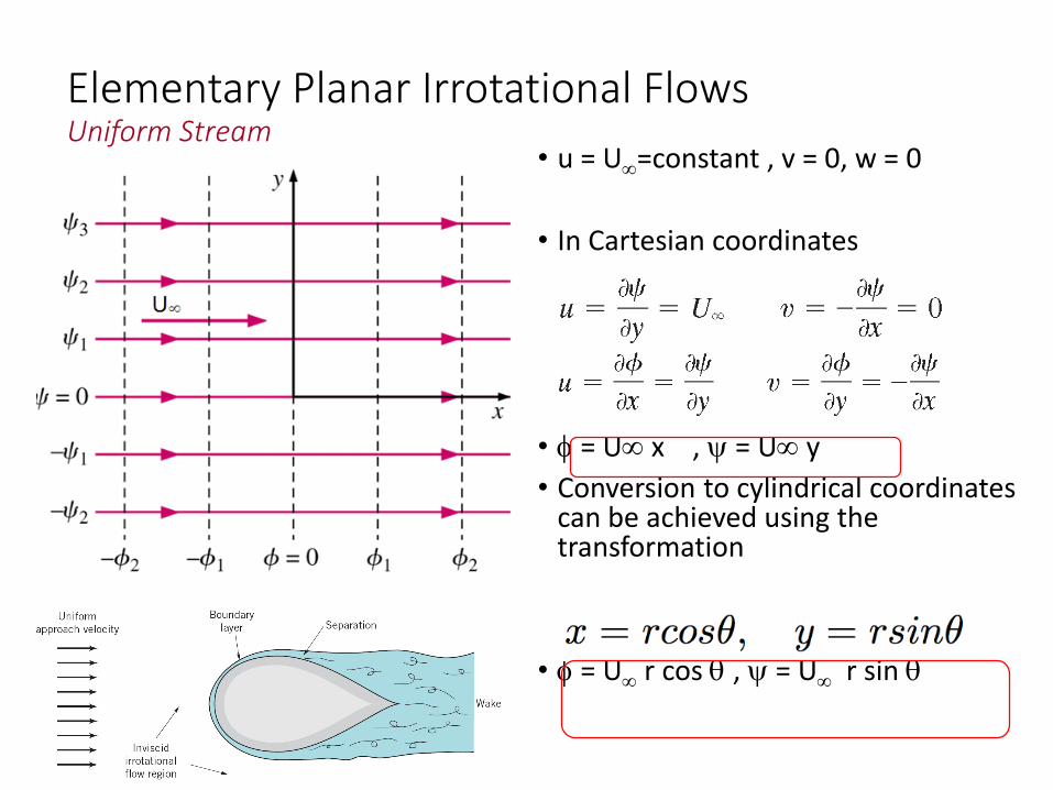
Elementary Planar Irrotational FlowsUniform Stream
• u = U=constant , v = 0, w = 0
• In Cartesian coordinates
• = U x , = U y
• Conversion to cylindrical coordinates can be achieved using the transformation
• = U r cos , = U r sin
U
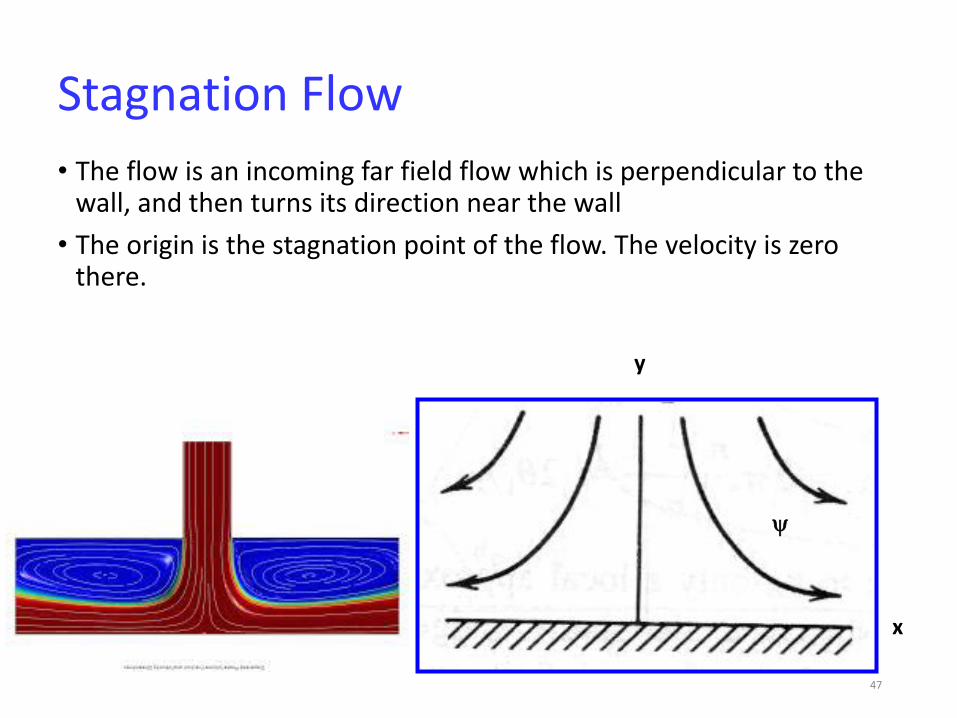
• The flow is an incoming far field flow which is perpendicular to the wall, and then turns its direction near the wall
• The origin is the stagnation point of the flow. The velocity is zero there.
Stagnation Flow
x
y
47
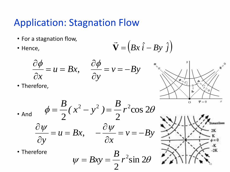
Application: Stagnation Flow
• For a stagnation flow,
• Hence,
• Therefore,
• And
• Therefore
2 cos22
222 rB
)yx(B
Byvy
Bxux
,
jByiBx ˆˆ V
2sin 2
2rB
Bxy
Byvx
Bxuy
,
48
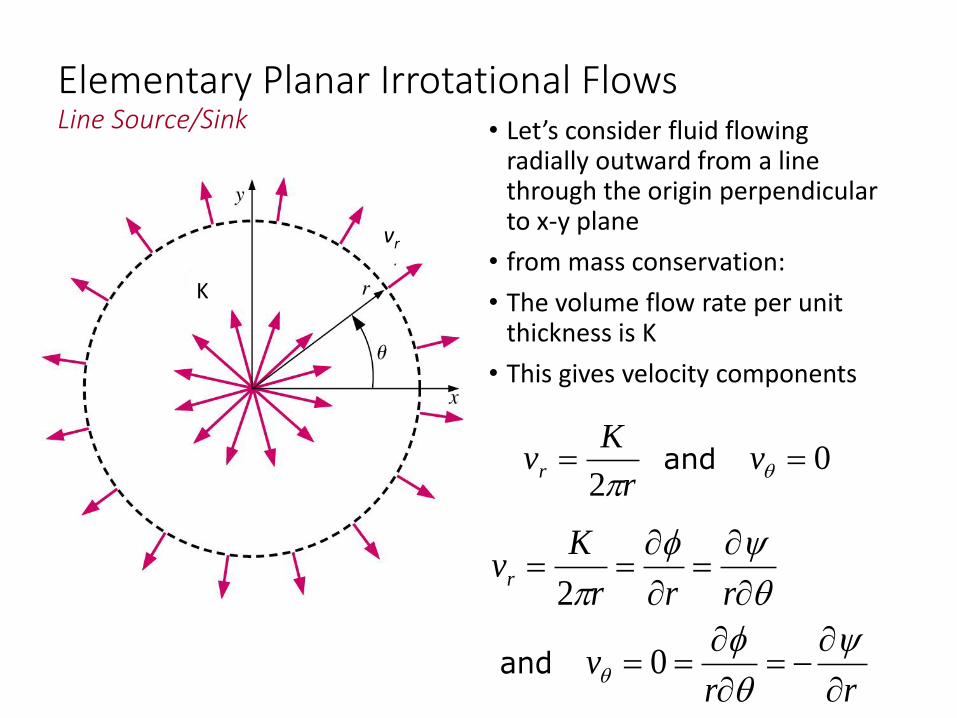
Elementary Planar Irrotational FlowsLine Source/Sink • Let’s consider fluid flowing
radially outward from a line through the origin perpendicular to x-y plane
• from mass conservation:
• The volume flow rate per unit thickness is K
• This gives velocity components
rrv
rrr
Kvr
0
2
and
0 2
vr
Kvr and
K
vr
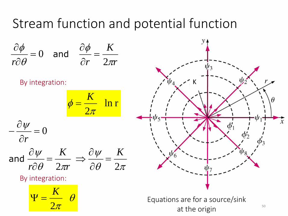
Stream function and potential function
2
0r
K
rr
and
By integration:
rln 2
K
2
2
0
K
r
K
r
r
and
By integration:
2
K Equations are for a source/sink
at the origin
K
50
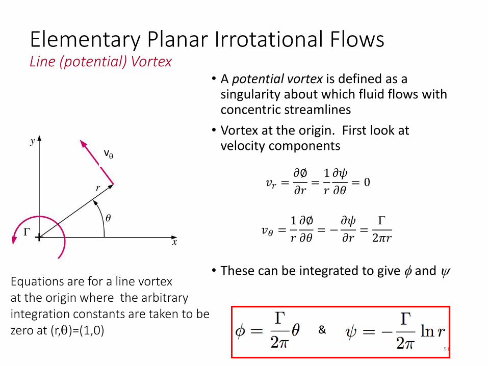
Elementary Planar Irrotational FlowsLine (potential) Vortex
• A potential vortex is defined as a singularity about which fluid flows with concentric streamlines
• Vortex at the origin. First look at velocity components
• These can be integrated to give and Equations are for a line vortexat the origin where the arbitrary integration constants are taken to be zero at (r,)=(1,0)
𝑣𝜃 =1
𝑟
𝜕∅
𝜕𝜃= −
𝜕𝜓
𝜕𝑟=
2𝜋𝑟
𝑣𝑟 =𝜕∅
𝜕𝑟=1
𝑟
𝜕𝜓
𝜕𝜃= 0
v
&
51
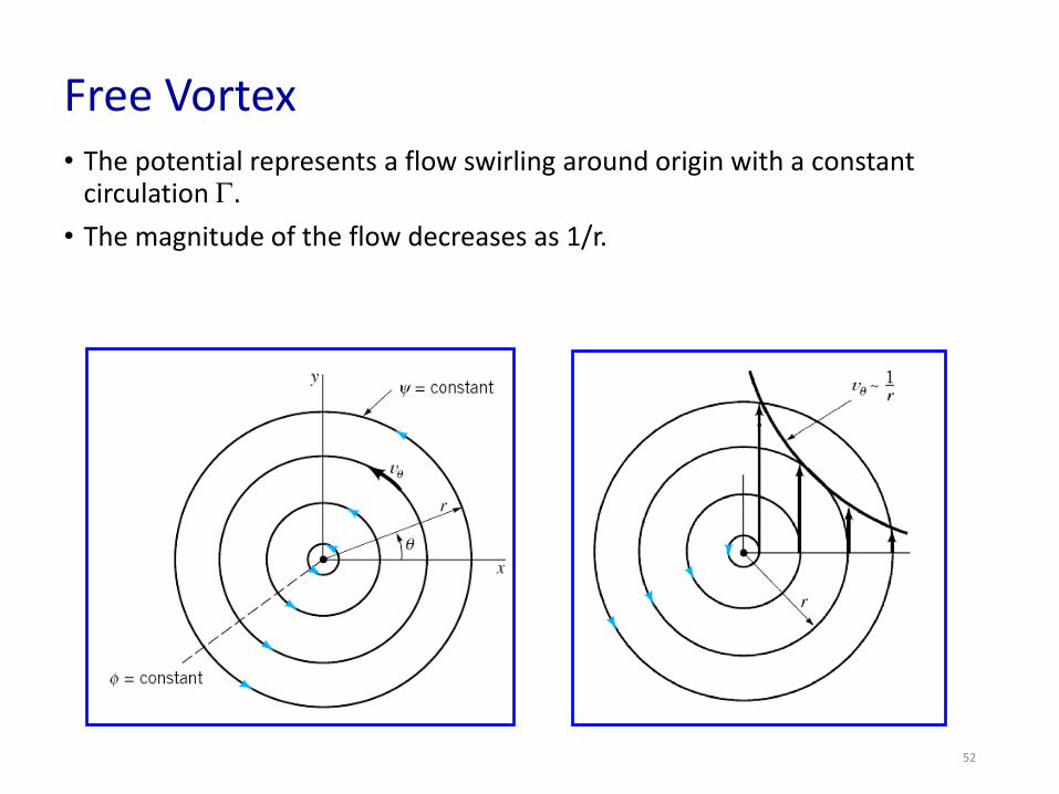
• The potential represents a flow swirling around origin with a constant circulation .
• The magnitude of the flow decreases as 1/r.
Free Vortex
52
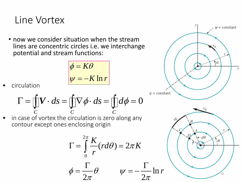
Line Vortex
• now we consider situation when the stream lines are concentric circles i.e. we interchange potential and stream functions:
ln
K
K r
• circulation
0C C C
ds ds d V
• in case of vortex the circulation is zero along any contour except ones enclosing origin
2
0
( ) 2
ln2 2
Krd K
r
r
53
54
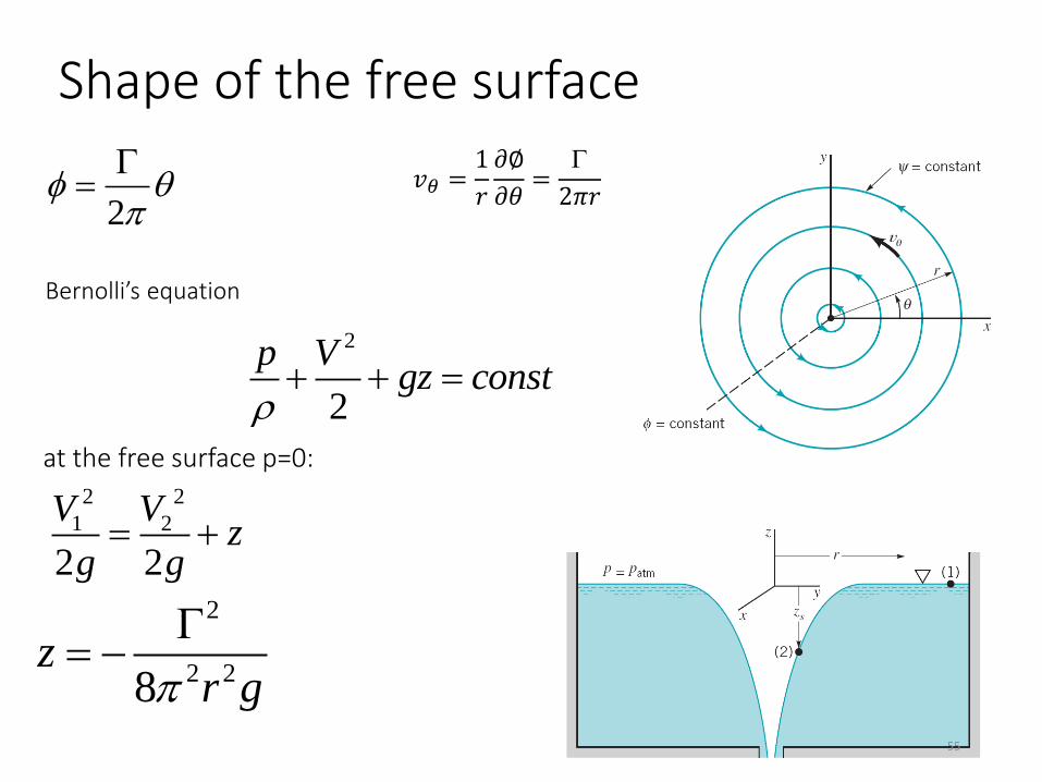
Shape of the free surface
2
2
2
p Vgz const
2 2
1 2
2 2
V Vz
g g
at the free surface p=0:
2
2 28z
r g
𝑣𝜃 =1
𝑟
𝜕∅
𝜕𝜃=
2𝜋𝑟
Bernolli’s equation
55
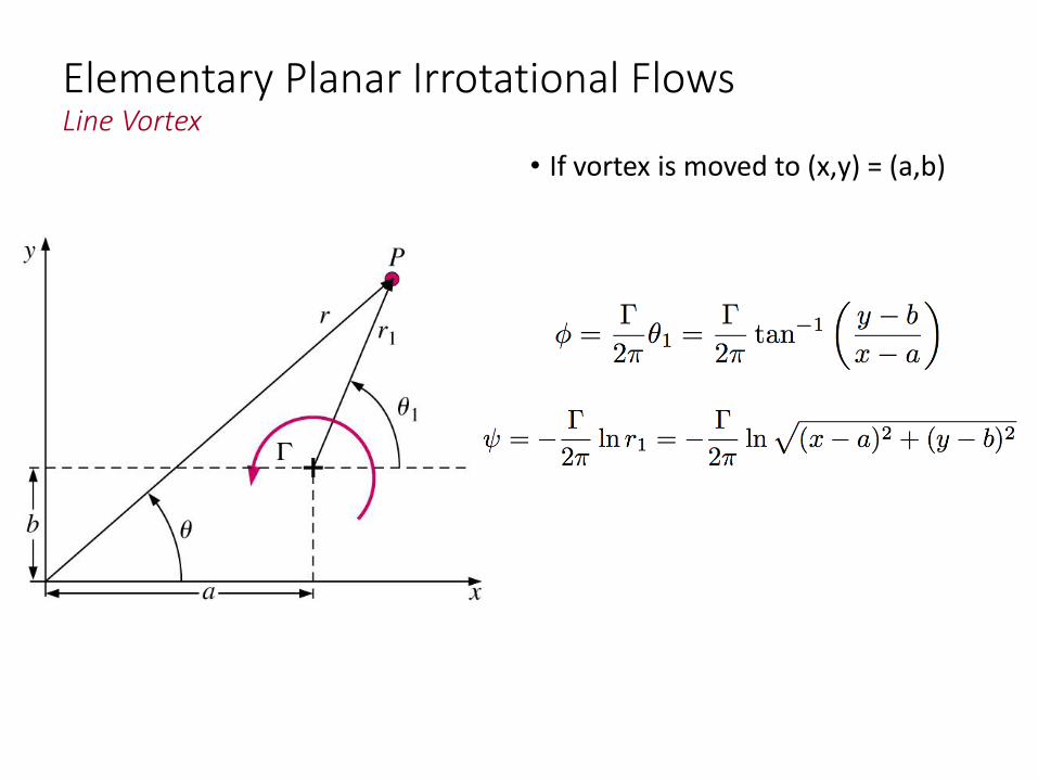
Elementary Planar Irrotational FlowsLine Vortex
• If vortex is moved to (x,y) = (a,b)
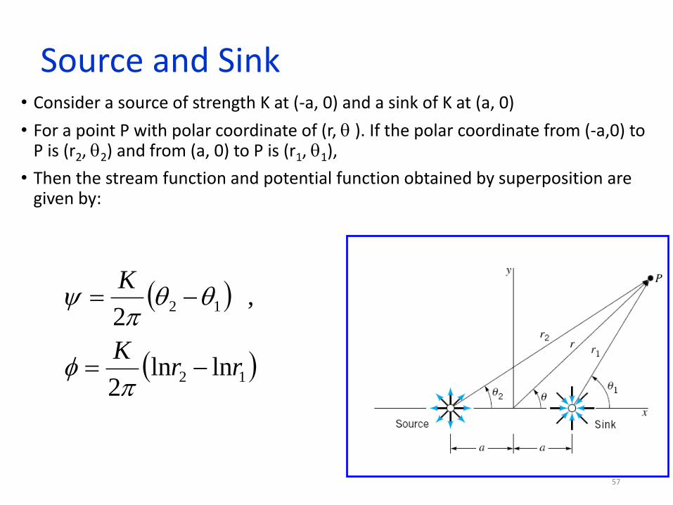
Source and Sink• Consider a source of strength K at (-a, 0) and a sink of K at (a, 0)
• For a point P with polar coordinate of (r, ). If the polar coordinate from (-a,0) to P is (r2, 2) and from (a, 0) to P is (r1, 1),
• Then the stream function and potential function obtained by superposition are given by:
12
12
lnln2
, 2
rrK
K
57
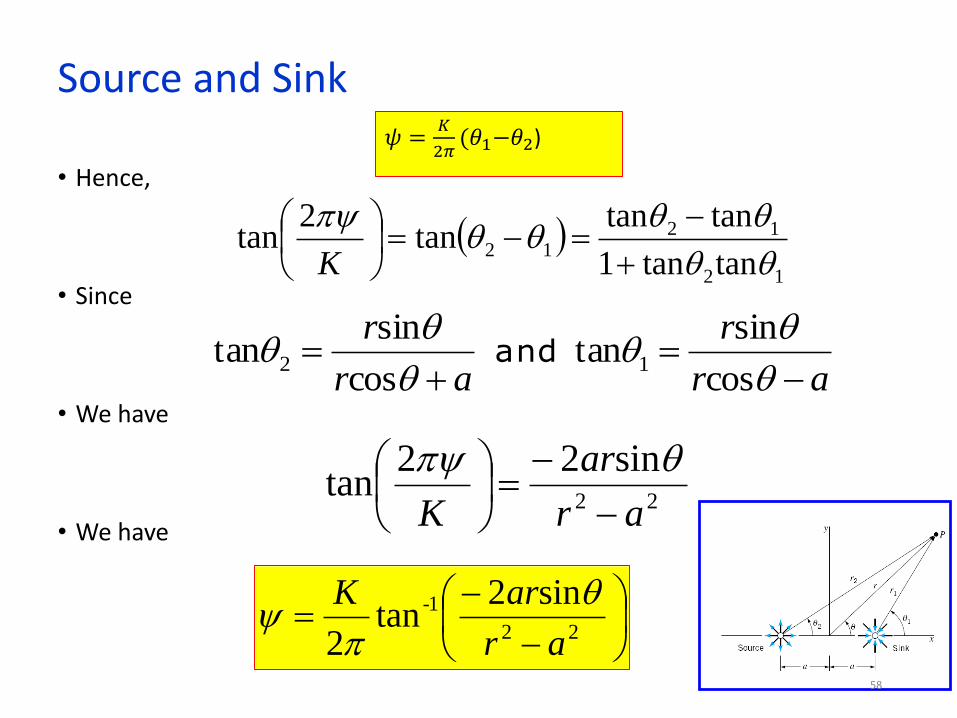
Source and Sink
• Hence,
• Since
• We have
• We have
12
1212
tantan1
tantantan
2tan
K
22
sin22tan
ar
ar
K
ar
r
ar
r
cos
sintan
cos
sintan 12 and
22
1- sin2tan
2 ar
arK
𝜓 =𝐾
2𝜋(𝜃1−𝜃2)
58
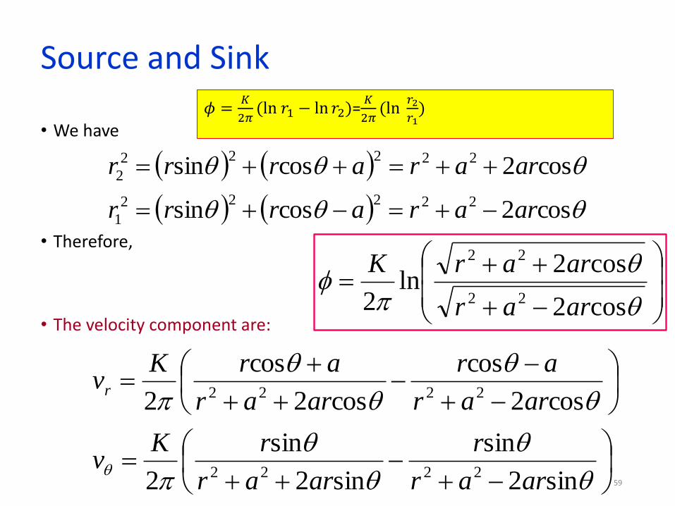
Source and Sink
• We have
• Therefore,
• The velocity component are:
cos2cossin
cos2cossin
22222
1
22222
2
arararrr
arararrr
cos2
cos2ln
2 22
22
arar
ararK
𝜙 =𝐾
2𝜋(ln 𝑟1 − ln 𝑟2)=
𝐾
2𝜋(ln
𝑟2
𝑟1)
sin2
sin
sin2
sin
2
cos2
cos
cos2
cos
2
2222
2222
arar
r
arar
rKv
arar
ar
arar
arKvr
59
60
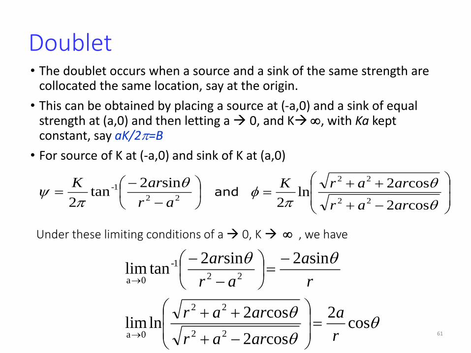
Doublet• The doublet occurs when a source and a sink of the same strength are
collocated the same location, say at the origin.
• This can be obtained by placing a source at (-a,0) and a sink of equal strength at (a,0) and then letting a 0, and K , with Ka kept constant, say aK/2=B
• For source of K at (-a,0) and sink of K at (a,0)
and sin2
tan2 22
1-
ar
arK
cos2
cos2ln
2 22
22
arar
ararK
Under these limiting conditions of a 0, K , we have
cos2
cos2
cos2lnlim
sin2sin2tanlim
22
22
0a
22
1-
0a
r
a
arar
arar
r
a
ar
ar
61
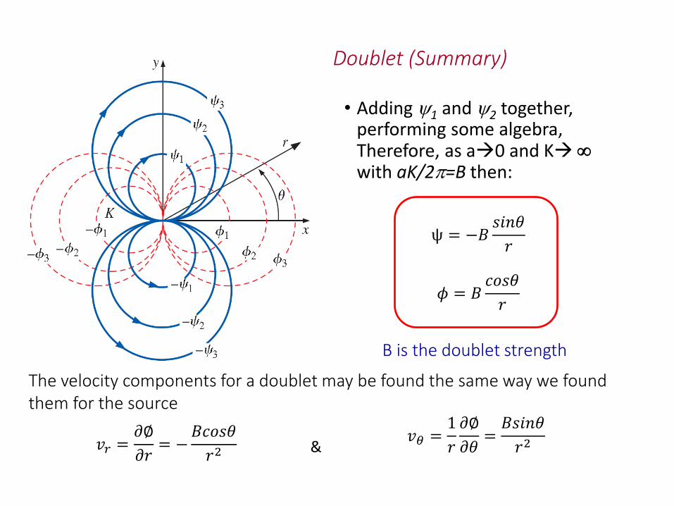
Doublet (Summary)
• Adding 1 and 2 together, performing some algebra, Therefore, as a0 and K with aK/2=B then:
B is the doublet strength
ψ = −𝐵𝑠𝑖𝑛𝜃
𝑟
𝜙 = 𝐵𝑐𝑜𝑠𝜃
𝑟
The velocity components for a doublet may be found the same way we found them for the source
𝑣𝑟 =𝜕∅
𝜕𝑟= −
𝐵𝑐𝑜𝑠𝜃
𝑟2𝑣𝜃 =
1
𝑟
𝜕∅
𝜕𝜃=𝐵𝑠𝑖𝑛𝜃
𝑟2&
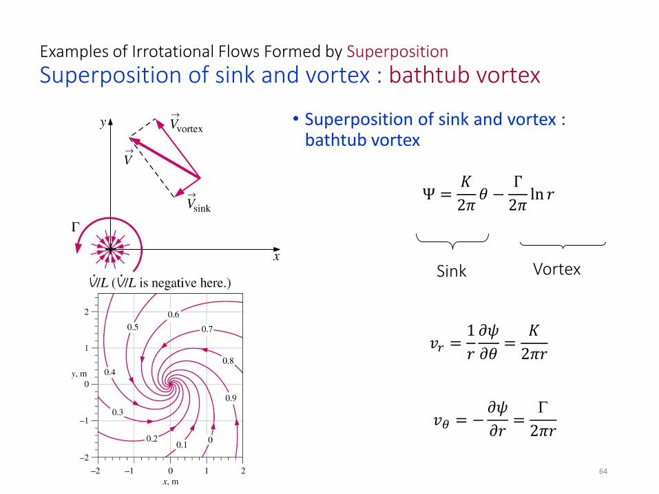
Examples of Irrotational Flows Formed by Superposition
Superposition of sink and vortex : bathtub vortex
• Superposition of sink and vortex : bathtub vortex
Sink Vortex
Ψ =𝐾
2𝜋𝜃 −
Γ
2𝜋ln 𝑟
𝑣𝜃 = −𝜕𝜓
𝜕𝑟=
2𝜋𝑟
𝑣𝑟 =1
𝑟
𝜕𝜓
𝜕𝜃=
𝐾
2𝜋𝑟
64
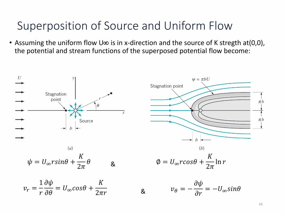
Superposition of Source and Uniform Flow• Assuming the uniform flow U is in x-direction and the source of K stregth at(0,0),
the potential and stream functions of the superposed potential flow become:
𝜓 = 𝑈∞𝑟𝑠𝑖𝑛𝜃 +𝐾
2𝜋𝜃 ∅ = 𝑈∞𝑟𝑐𝑜𝑠𝜃 +
𝐾
2𝜋ln 𝑟&
𝑣𝑟 =1
𝑟
𝜕𝜓
𝜕𝜃= 𝑈∞𝑐𝑜𝑠𝜃 +
𝐾
2𝜋𝑟𝑣𝜃 = −
𝜕𝜓
𝜕𝑟= −𝑈∞𝑠𝑖𝑛𝜃&
65
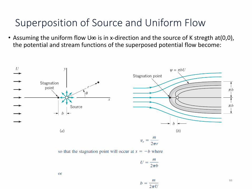
Superposition of Source and Uniform Flow• Assuming the uniform flow U is in x-direction and the source of K stregth at(0,0),
the potential and stream functions of the superposed potential flow become:
66
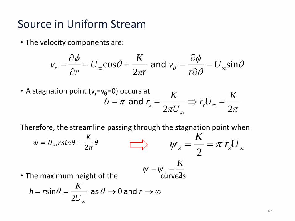
Source in Uniform Stream
• The velocity components are:
• A stagnation point (vr=v=0) occurs at
Therefore, the streamline passing through the stagnation point when
• The maximum height of the curve is
sin
2cos
U
rv
r
KU
rvr and
22
KUr
U
Kr ss
and
UrK
ss 2
2
Ks
and as rU
Krh 0
2sin
𝜓 = 𝑈∞𝑟𝑠𝑖𝑛𝜃 +𝐾
2𝜋𝜃
67
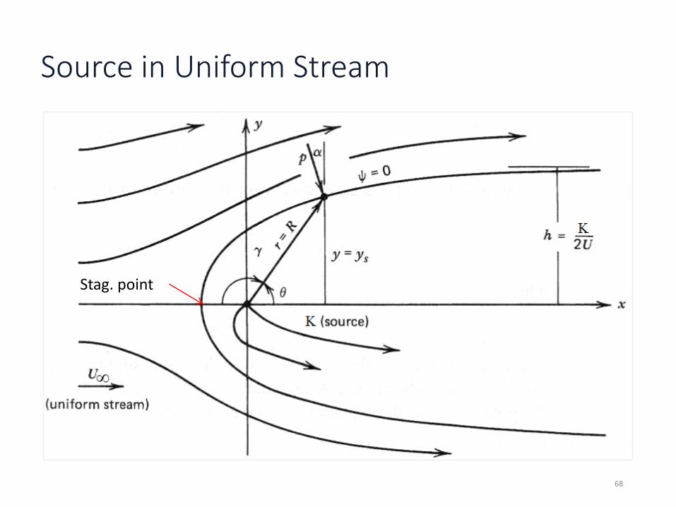
Source in Uniform Stream
2
mψ
2
mψ
0ψStag. point
68
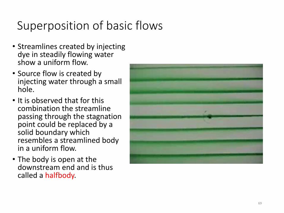
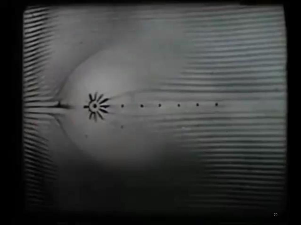
Superposition of basic flows
• Streamlines created by injecting dye in steadily flowing water show a uniform flow.
• Source flow is created by injecting water through a small hole.
• It is observed that for this combination the streamline passing through the stagnation point could be replaced by a solid boundary which resembles a streamlined body in a uniform flow.
• The body is open at the downstream end and is thus called a halfbody.
69
70
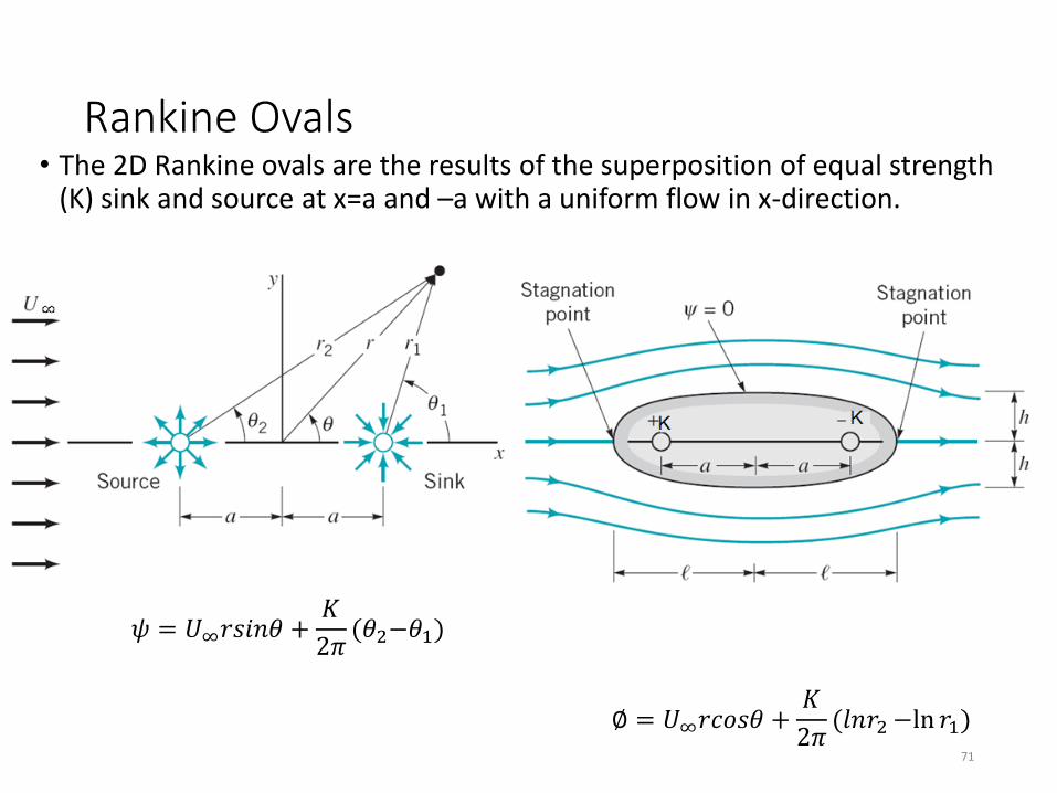
Rankine Ovals• The 2D Rankine ovals are the results of the superposition of equal strength
(K) sink and source at x=a and –a with a uniform flow in x-direction.
𝜓 = 𝑈∞𝑟𝑠𝑖𝑛𝜃 +𝐾
2𝜋(𝜃2−𝜃1)
∅ = 𝑈∞𝑟𝑐𝑜𝑠𝜃 +𝐾
2𝜋(𝑙𝑛𝑟2−ln 𝑟1)
71
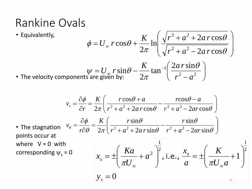
Rankine Ovals• Equivalently,
• The velocity components are given by:
• The stagnation
points occur at
where V = 0 with
corresponding s = 0
22
1
22
22
sin2tan
2sin
cos2
cos2ln
2cos
ar
raKrU
raar
raarKrU
sin2
sin
sin2
sin
2
cos2
cos
cos2
cos
2
2222
2222
arar
r
raar
rK
rv
arar
ar
raar
arK
rvr
0
12
1
2
1
2
s
ss
y
aU
K
a
xa
U
Kax
i.e., ,
72
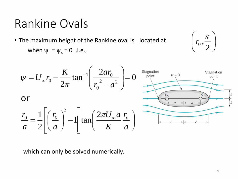
Rankine Ovals• The maximum height of the Rankine oval is located at
when = s = 0 ,i.e.,
which can only be solved numerically.
20
,r
a
r
K
aU
a
r
a
r
ar
arKrU
o0
2tan1
2
1
02
tan2
2
0
22
0
01
0
or
73
74
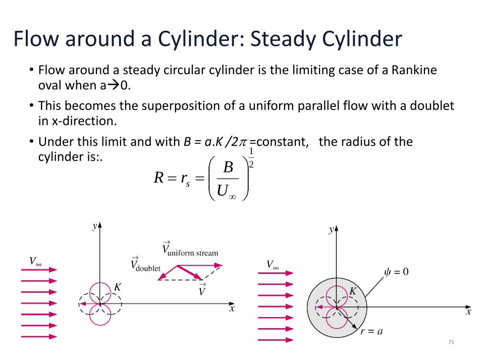
Flow around a Cylinder: Steady Cylinder• Flow around a steady circular cylinder is the limiting case of a Rankine
oval when a0.
• This becomes the superposition of a uniform parallel flow with a doublet in x-direction.
• Under this limit and with B = a.K /2 =constant, the radius of the cylinder is:.
2
1
U
BrR s
75
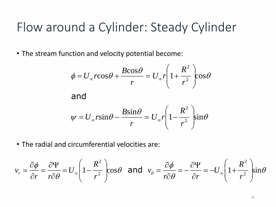
• The stream function and velocity potential become:
• The radial and circumferential velocities are:
sin1sin
sin
cos1cos
cos
2
2
2
2
r
RrU
r
BrU
r
RrU
r
BrU
and
sin1 cos1
2
2
2
2
r
RU
rrv
r
RU
rrvr and
Flow around a Cylinder: Steady Cylinder
76
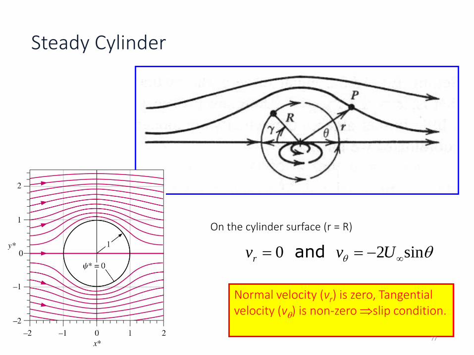
Steady Cylinder
On the cylinder surface (r = R)
Normal velocity (vr) is zero, Tangential velocity (v) is non-zero slip condition.
sin2 0 Uvvr and
77
78
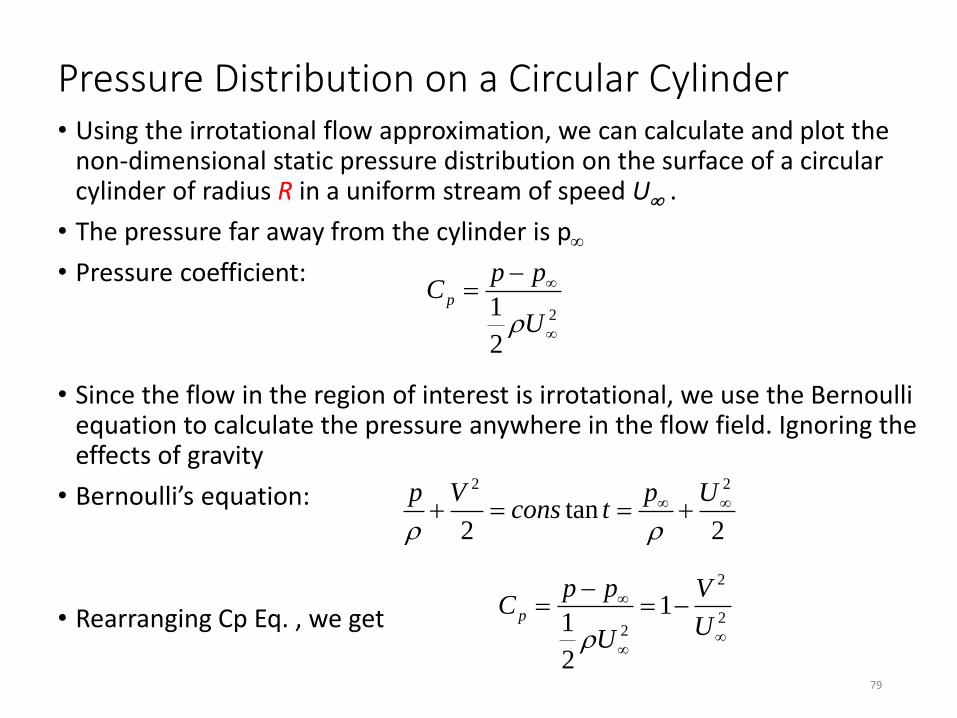
Pressure Distribution on a Circular Cylinder• Using the irrotational flow approximation, we can calculate and plot the
non-dimensional static pressure distribution on the surface of a circular cylinder of radius R in a uniform stream of speed U .
• The pressure far away from the cylinder is p• Pressure coefficient:
• Since the flow in the region of interest is irrotational, we use the Bernoulli equation to calculate the pressure anywhere in the flow field. Ignoring the effects of gravity
• Bernoulli’s equation:
• Rearranging Cp Eq. , we get
2
2
1
U
ppC p
2tan
2
22
Up
tconsVp
2
2
2
1
2
1
U
V
U
ppC p
79
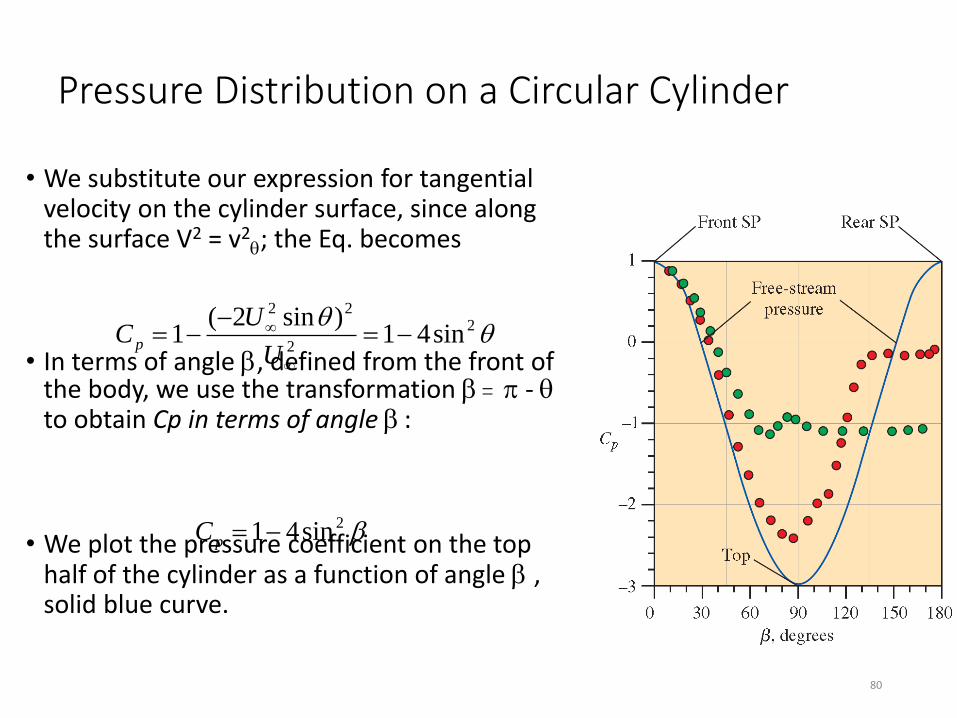
Pressure Distribution on a Circular Cylinder
• We substitute our expression for tangential velocity on the cylinder surface, since along the surface V2 = v2
; the Eq. becomes
• In terms of angle , defined from the front of the body, we use the transformation = - to obtain Cp in terms of angle :
• We plot the pressure coefficient on the top half of the cylinder as a function of angle , solid blue curve.
2
2
22
sin41)sin2(
1
U
UC p
2sin41pC
80
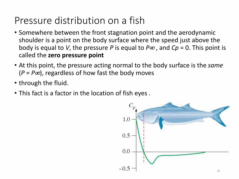
Pressure distribution on a fish• Somewhere between the front stagnation point and the aerodynamic
shoulder is a point on the body surface where the speed just above the body is equal to V, the pressure P is equal to P , and Cp = 0. This point is called the zero pressure point
• At this point, the pressure acting normal to the body surface is the same (P = P), regardless of how fast the body moves
• through the fluid.
• This fact is a factor in the location of fish eyes .
81
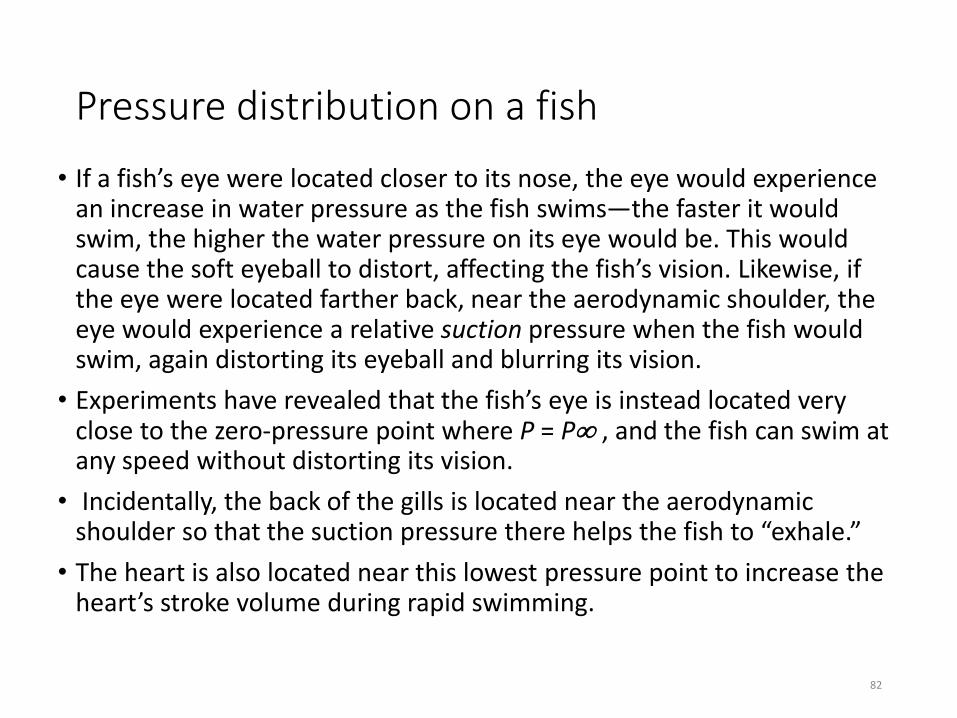
• If a fish’s eye were located closer to its nose, the eye would experience an increase in water pressure as the fish swims—the faster it would swim, the higher the water pressure on its eye would be. This would cause the soft eyeball to distort, affecting the fish’s vision. Likewise, if the eye were located farther back, near the aerodynamic shoulder, the eye would experience a relative suction pressure when the fish would swim, again distorting its eyeball and blurring its vision.
• Experiments have revealed that the fish’s eye is instead located very close to the zero-pressure point where P = P , and the fish can swim at any speed without distorting its vision.
• Incidentally, the back of the gills is located near the aerodynamic shoulder so that the suction pressure there helps the fish to “exhale.”
• The heart is also located near this lowest pressure point to increase the heart’s stroke volume during rapid swimming.
Pressure distribution on a fish
82
Reading Material
• Chapter 6 of Munson (Sections 6.4 to 6.7)
83