2017Fellowship Symposium, 8 May 2017, Weber State University

Implementation of OpenFOAM for Inviscid,Incompressible Aerodynamic Flows

Jackson T. Reid∗ and Douglas F. Hunsaker†

Utah State University, Logan, Utah, 84321, USA

Abstract

This paper is the description of the Utah State University AeroLab’s AerodynamicCenter Analysis Tool (AeroCAT), which is an implementation of the OpenFOAM CFDtoolbox. AeroCAT takes in a user input file, generates a mesh, and solves a steady,inviscid, incompressible flow, automatically repeating the process for a range of angles ofattack. It then processes the results to predict the wing’s span-wise locus of aerodynamiccenters. The mesh generator used in this tool is GridX, developed by a former PhDstudent at USU, and the CFD solver is OpenFOAM.

Nomenclature

x Axis from leading to trailing edge ofthe root airfoil

y Axis perpendicular to root chord line in theroot airfoil plane

z Axis span-wise along a wing, perpendicularto both the x and y axes

i Cell index from wing root to tipj Cell index around each cross-sectionk Cell index radially from wing to boundaryα Angle of Attack, deg or radcref Length of the root airfoil’s chordxac x location of the aerodynamic centeryac y location of the aerodynamic centerCm,ac Coefficient of moment about the aero-

dynamic centerCN Coefficient of the normal force (y direction)CA Coefficient of the axial force (x direction)Cm Coefficient of moment about the leading edgeCN,α Derivative of CN with respect to αCA,α Derivative of CA with respect to αCm,α Derivative of Cm with respect to αCN,α,α Derivative of CN,α with respect to αCA,α,α Derivative of CA,α with respect to αCm,α,α Derivative of Cm,α with respect to α

∗Graduate Research Assistant, Mechanical & AerospaceEngineering, 4130 Old Main Hill

†Assistant Professor, Mechanical & Aerospace Engineering,4130 Old Main Hill

I. Introduction

The AeroLab at Utah State University (USU) isdedicated to discovering and publishing fundamen-tal aerodynamic principles. 1 As such, we activelywork to develop open-source tools that will help us,and others, in aerodynamic design, analysis, and op-timization. In order to perform this research and de-velopment, it was necessary to both have a means togather data—to observe trends and create empiricalequations—and have a manner in which to validatepotential flow and other aerodynamics models devel-oped by the lab. To this end, the Aerodynamic Cen-ter Analysis Tool (AeroCAT) was developed. Initiallydesigned to run CFD simulation of steady, inviscid,incompressible flow over wings and airfoils, then cal-culating the span-wise locus of aerodynamic centers,AeroCAT is also capable of providing spanwise liftdistribution data to validate our aerodynamic mod-els against.

II. Tool Overview

AeroCAT begins with a .json input file that con-tains mesh specifications, and simulation settings. Be-cause this tool is meant to be user friendly and sim-ple to run, not all possible settings are available inthis input file, but rather are hard-coded into thesource script. AeroCAT takes in the values from theinput file and generates a mesh using GridX. Then,that mesh is used in an OpenFOAM simulation of the

1AeroLab Mission Statement as seen on aero.usu.edu

1 of 17

Utah NASA Space Grant Consortium 2017

flow. The forces and moments on the airfoil or wingare recorded by OpenFOAM automatically to be usedin post-processing routines. The process is then re-peated for the next angle of attack, and continuesthroughout the range of angles of attack specified bythe user.

A new mesh is generated for each angle of attackin the desired range because GridX uses a trailingedge streamline approximation to position the cellsbehind the aerodynamic surface. Once all angles ofattack have been simulated and all the data collected,AeroCAT post-processes the collection, calculatingthe locus of aerodynamic centers and lift distribu-tions, plotting them for easy visualization. The spe-cific details of this process, as well as a description ofall the setting options, is found in the sections here-after.

AeroCAT has been developed using a Linux oper-ating system and, as such, the following descriptionswill be have only been tested using Linux. That be-ing said, it is not expected that there be major issuestrying to run AeroCAT on other operating systems.

II.A. Installation and Input Files

The installation AeroCAT is performed in two stages.First OpenFOAM must be installed by following theinstructions on its website. 2 The next step is torun the shell script “Compile.sh”, which compiles theFORTRAN files needed for GridX and the post pro-cessing subroutines, creates the needed executables,and sets the necessary permissions for the Pythonscripts. The installation is then complete. 3

AeroCAT should be installed in a location eas-ily accessible to the user and run in a terminal withthe OpenFOAM system variables set [1]. As it runs,AeroCAT creates a folder in the installation direc-tory containing the mesh, configure files, and resultsof each project. OpenFOAM requires certain systemvariables to be set before runtime, and thus AeroCATcannot be run without those variables.

When running AeroCAT, the user is first askedwhether there is an existing input file to be used. Ifthe user has an input file to use, it is specified. On theother hand, AeroCAT will walk the user through thecreation of an input file that is then saved and can bereused or edited for future projects. An example ofan AeroCAT input file is included in the Appendix.

AeroCAT uses a .json format for its input file sowhile the order of the elements is not important, ingeneral all elements should be included in the inputfile to avoid runtime errors. The name of the in-put file (exluding the .json extension) becomes the

2As of 21 April 2017: www.openfoam.com/download3To generate plots while running GridX as a stand alone

program, PlotMTV must be installed as well.

project name off which all other files and folders arenamed. For example, if the input file were named“Test1.json”, AeroCAT would create (or write over)a folder named “Test1”, and, subsequently, save theOpenFOAM simulation files for an angle of attack αin a folder named “Test1_α”.

The specific elements of the AeroCAT input filewill be described in more detail in their correspondingsections further down.

II.B. Mesh Generator

The mesh generator used by AeroCAT, GridX, wasdeveloped by Professor Warren Phillips and Nick Al-ley during Nick’s PhD work here at Utah State. It isuseful due to the range of airfoils and finite wings it iscapable of generating, as well as the user’s ability toadjust the cell spacing. The original version of GridXdid not have compatibility with OpenFOAM, so partof the development of AeroCAT was the addition offunctions that will produce the appropriate mesh andcase files to run an OpenFOAM simulation.

II.B.1. Stand-Alone Walk-Through

Using AeroCAT, GridX is run automatically from themain AeroCAT script. However, the following is adescription of GridX being run as a stand-alone pro-gram. This will be of use to the reader, as it willdemonstrate what is happening in the background ofAeroCAT and provide insight as to how to modifythe mesh settings in a more advanced way.

GridX is initiated by running the executable “In-ner.out” in a directory that contains a GridX inputfile,“*.iGridX”. GridX asks for the name of the inputfile, without extension, and then reads that file, cre-ates an airfoil based on the settings read in, calculatesthe trailing edge streamline, and then displays the“MENU”. This menu shows all the settings that arecurrently active in GridX, including: output file for-mats, flight state information, airfoil and wing data,and grid properties. These options can be modifiedby the user by entering the code displayed next to theoption and then following the instructions displayedin the terminal.

Once all the options are set as desired, the code“gg” is entered to begin the grid generation. GridXstarts by creating splines of the airfoil, trailing edgestreamline, and outer boundary. These splines will beused by the generator as boundary points to smooththe mesh algebraically or by an elliptic partial differ-ential equation. This smoothing ensures that the ofa cell gradually grows or shrinks as it transitions tothe next cell. In the case of a 3D simulation, GridXstarts at the symmetry plane, which corresponds tothe root airfoil of the wing, and generates that pla-

2 of 17

Utah NASA Space Grant Consortium 2017

nar grid. For the 2D case, this is the end of the gridgeneration. In both the 3D and 2D cases at this timeGridX asks the user if he or she would like to view aplot of the mesh, first of the boundary layer grid andthen of the transition and full planar grids.

GridX then generates and connects planar gridsspan-wise along the z direction. These grids are par-allel (or at least very close) to one another until theendcap of the wing is reached. Sweep and dihedralin the wing is handled by a translation of these par-allel grids in either the y or x directions. Once theendcap is reached, the planar grids begin to fold inhalf about the leading and trailing edge streamlinesof the tip airfoil. The final planar grid is folded com-pletely in half such that the points that make up thetop and bottom halves are identical. The duplicatedpoints along this plane are consolidated during thewriting of the OpenFOAM mesh files.

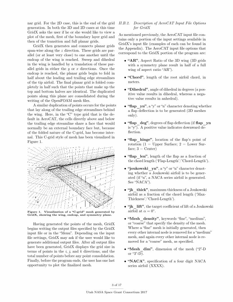
A similar duplication of points occurs for the pointsthat lay along of the trailing edge streamlines behindthe wing. Here, in the “C” type grid that is the de-fault in AeroCAT, the cells directly above and belowthe trailing edge streamline share a face that wouldnormally be an external boundary face but, becauseof the folded nature of the C-grid, has become inter-nal. This C-grid style of mesh has been visualized inFigure 1.

Figure 1. Visualization of a “C-grid” mesh generated byGridX, showing the wing, endcap, and symmetry plane.

Having generated the points of the mesh, GridXbegins writing the output files specified by the GridXinput file or in the “Menu”. Depending on the inputfile settings, GridX may ask if the user would like togenerate additional output files. After all output fileshave been generated, GridX displays the grid size interms of points in the i, j, and k directions, and thetotal number of points before any point consolidation.Finally, before the program ends, the user has one lastopportunity to plot the finalized mesh.

II.B.2. Description of AeroCAT Input File Optionsfor GridX

As mentioned previously, the AeroCAT input file con-tains only a portion of the input settings available inGridX’s input file (examples of each can be found inthe Appendix). The AeroCAT input file options thatcorrespond to the GridX portion of the program are:

• “AR” , Aspect Ratio of the 3D wing (3D gridswith a symmetry plane result in half of a fullwing of aspect ratio “AR”).

• “Chord” , length of the root airfoil chord, inmeters.

• “Dihedral” , angle of dihedral in degrees (a pos-itive value results in dihedral, whereas a nega-tive value results in anhedral).

• “flap_yn” , a “y” or “n” character denoting whethera flap deflection is to be generated (2D meshesonly).

• “flap_deg” , degrees of flap deflection (if flap_ynis “y”). A positive value indicates downward de-flection.

• “flap_hinge” , location of the flap’s point ofrotation (1 = Upper Surface; 2 = Lower Sur-face; 3 = Center)

• “flap_len” , length of the flap as a fraction ofthe chord length (‘Flap-Length’/’Chord-Length’).

• “joukowski_yn” , a “y” or “n” character denot-ing whether a Joukowski airfoil is to be gener-ated (if “n”, a NACA series airfoil is generated.See “NACA”).

• “jk_thick” , maximum thickness of a Joukowskiairfoil as a fraction of the chord length (‘Max-Thickness’/’Chord-Length’).

• “jk_lift” , the target coefficient of lift of a Joukowskiairfoil at α = 0◦.

• “Mesh_density” , keywords “fine”, “medium”,or “coarse” that specify the density of the mesh.Where a “fine” mesh is initially generated, thenevery other internal node is removed for a “medium”mesh, and again every other internal node is re-moved for a “coarse” mesh, as specified.

• “Mesh_dim” , dimension of the mesh (“2”-Dor “3”-D).

• “NACA” , specification of a four digit NACAseries airfoil (XXXX).

3 of 17

Utah NASA Space Grant Consortium 2017

• “Semi_span” , length of the 3D wing from cen-terline to tip along the z axis, in meters.

• “Sweep” , angle of sweep in degrees (a positivevalue results in a swept back wing, whereas anegative value results in a wing with forwardsweep).

• “TR” , Taper Ratio between the length of theroot chord length and the tip chord length (”Tip-Chord”/“Root-Chord”).

• “Washout” , angle of washout in degrees (a pos-itive value results in a tip with lower α than theroot, whereas a negative value results in a tipwith a higher α).

• “chord_bl3ff” , distance between the bound-ary layer cells and the outer boundary, in num-ber of chord lengths.

• “node_airfoil” , number of nodes on the airfoilsurface.

• “node_behind” , number of nodes located alongthe trailing edge streamline behind the wing.

• “node_bl2ff” , number of nodes located be-tween the boundary layer and outer boundaryabove, below, and in front of the wing.

• “node_boundary” , number of nodes in theboundary layer.

• “node_endcap” , number of span-wise nodeson each half of the endcap (“node_endcap” ontop, and “node_endcap” on bottom).

• “thickness1_bl” , thickness of the first bound-ary layer cell, as a fraction of the root chordlength (measured perpendicular to the wing/air-foil surface).

The settings “AoA_max” and “AoA_min” in theAeroCAT input file dictate the range of angle of at-tack, in degrees, for which simulations will be run, sothey also indirectly correspond to GridX input val-ues.

There are many other settings and ways to cus-tomize a mesh using GridX, but all of the most nec-essary settings are available through the AeroCATinput file. If there is an occasion that calls for themodification of settings not found in that file (e.g. ifcells are crossing and the right and left hand influ-ence parameters need adjusting), the user may man-ually modify the default values found in the “Aero-CAT_Main.py” script.

II.C. OpenFOAM

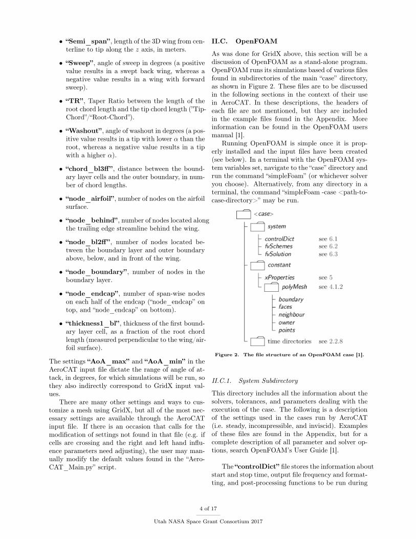
As was done for GridX above, this section will be adiscussion of OpenFOAM as a stand-alone program.OpenFOAM runs its simulations based of various filesfound in subdirectories of the main “case” directory,as shown in Figure 2. These files are to be discussedin the following sections in the context of their usein AeroCAT. In these descriptions, the headers ofeach file are not mentioned, but they are includedin the example files found in the Appendix. Moreinformation can be found in the OpenFOAM usersmanual [1].

Running OpenFOAM is simple once it is prop-erly installed and the input files have been created(see below). In a terminal with the OpenFOAM sys-tem variables set, navigate to the “case” directory andrun the command “simpleFoam” (or whichever solveryou choose). Alternatively, from any directory in aterminal, the command “simpleFoam -case <path-to-case-directory>” may be run.

Figure 2. The file structure of an OpenFOAM case [1].

II.C.1. System Subdirectory

This directory includes all the information about thesolvers, tolerances, and parameters dealing with theexecution of the case. The following is a descriptionof the settings used in the cases run by AeroCAT(i.e. steady, incompressible, and inviscid). Examplesof these files are found in the Appendix, but for acomplete description of all parameter and solver op-tions, search OpenFOAM’s User Guide [1].

The “controlDict” file stores the information aboutstart and stop time, output file frequency and format-ting, and post-processing functions to be run during

4 of 17

Utah NASA Space Grant Consortium 2017

execution. The following is a list of the needed en-tries for this file and a brief description of each. Anexample “controlDict” file is located in the Appendix.

• “application” , the name of the solver to beused for the case. “simpleFoam” will be usedfor AeroCAT.

• “startFrom” , the time (or pseudo-time in steadyflows) at which the solver should begin. The de-fault is “startTime” (described below), though“firstTime” and “lastTime” are options. Thesetwo options are based on the time subdirecto-ries found in the main “case” directory. “first-Time” begins the simulation from the informa-tion in the earliest time subdirectory, whereas“lastTime” starts the solver with the data in thelast time subdirectory. Thus, to restart a solverfrom where it left off, the “lastTime” option isselected.

• “startTime” , the time at which the solver shouldbegin if the “startFrom startTime” option is se-lected. The default for this field is “0”.

• “stopAt” , the time at which the solver shouldend. The option used by AeroCAT here is “end-Time”. For more options see the User Guide [1].

• “endTime” , the time at which the solver shouldend when the option “stopAt stopTime” is se-lected.

• “deltaT” , the time step (or pseudo-time step)of the simulation.

• “writeControl” , the units assigned to “writeIn-terval” (described below), controlling the fre-quency at which data is written. The defaultis “timeStep”, which sets the units to numberof time steps (as defined by “deltaT”). Otheroptions include “runTime”, for units of secondsof simulated time, “cpuTime”, for units of sec-onds of CPU time, and “clockTime”, for unitsof seconds of real time.

• “writeInterval” , the frequency at which datais written to a new time subdirectory through-out the simulation. It has units that are definedby “writeControl”.

• “purgeWrite” , the number of time subdirecto-ries to remain in the “case” directory, excludingthe starting time subdirectory. For example, if“purgeWrite” is equal to five, OpenFOAM willcyclically delete the oldest time subdirectorythroughout the course of the simulation, main-taining the five most recent (and the initial)subdirectories. The default for “purgeWrite” iszero, meaning all time subdirectories are kept.

• “writeFormat” , the specification of “ascii” or“binary” format for the output files.

• “writePrecision” , the number of significantfigures used in the data files.

• “writeCompression” , the “on” or “off” speci-fication of whether the files are compressed toa “.zip” folder when written.

• “timeFormat” , the format for naming the timesubdirectories. The options include: “fixed”(x.xxxxxx), “scientific” (x.xxxxxxexx), or “gen-eral” which changes between “fixed” and “gen-eral” depending on the scientific exponent of thetime value and the value specified by “timePre-cision”.

• “timePrecision” , the maximum number of dig-its after the decimal point in time subdirectorynames.

• “runTimeModifiable” , the switch that, if“true”, tells OpenFOAM to re-read the inputfiles at the beginning of each time-step, allow-ing for in-simulation modification of parametersand values.

After the above entries, there is an optional “func-tions” directory. In the example found in the Ap-pendix there are two entries, “#includeFunc resid-uals” and “#includeFunc forceCoeffsIncompressible”.These entries are run-time functions that calculateand output residual and force (lift, drag, and mo-ment) coefficients, respectively, during the simula-tion. The result is a new subdirectory, “postProcess-ing”, in the “case” directory that contains a data filefor each function storing the progression of the de-sired values throughout the course of the simulation.There are many additional functions that may be in-cluded here, and the reader can find a list of these inOpenFOAM’s User Guide [1].

The “fvSchemes” file houses the definitions forthe numerical schemes to be used to calculate eachpart of the underlying equations. An example of thisfile may be found in the Appendix. Again, there aremany options for each of these entries, but those dis-played here are the ones that have been found to workbest for “simpleFoam” in the applications of Aero-CAT.

The “default” entry in each category is the settingused if nothing is set explicitly below it. In theseschemes, “Gauss” refers to finite volume discretiza-tion of Gaussian integration. This discretization re-quires values be interpolated from the cell centers tothe cell faces [1]. In the schemes used here, “linear”

5 of 17

Utah NASA Space Grant Consortium 2017

interpolation, or central differencing, is used almostexclusively.

• “ddtSchemes” , the calculation of derivativeswith respect to time. Because this is a steadysimulation, “steadyState” is used and timederivatives are set to zero.

• “gradSchemes” , the calculation of the gradi-ent, “∇”. “Gauss linear” is the default used here.

• “divSchemes” , the calculation of the diver-gence, “∇·”. “Gauss linear” is the default, but“bounded Gauss linearUpwind grad(U)” is spec-ified for the “div(phi,U)” term ( ∇ · (φU) =∇ · (ρUU) ).In this scheme, the “bounded” refers to the treat-ment of the ∇ ·U term the material derivative.For incompressible flows, this term equals zeroat convergence, but may not equal zero beforeconvergence is reached. So, the “bounded” termin this scheme solves for the∇·U term through-out the simulation.This scheme also uses “linearUpwind grad(U)”instead of “linear”. The “linearUpwind” termcalls for a weighted interpolation scheme thatfavors upwind values. The “linearUpwind” op-tion requires that the discretization of the ve-locity gradient be specified, so the “grad(U)”term is referencing the discretization scheme forthe velocity specified under “gradSchemes”. (Inthis case it takes on the “default” “gradSchemes”value.) [1]

• “laplacianSchemes” , the calculation of theLaplacian, “∇2”. “Gauss linear corrected” isused for this scheme. Here, the “corrected” termis a “snGradScheme” scheme and will be de-scribed below.

• “interpolationSchemes” , the calculation ofvalues at a cell face through interpolation ofcell-centered values. The “linear” interpolationscheme is used.

• “snGradSchemes” , the calculation of the gra-dient, ∇, normal to a cell face. Here a “cor-rected” scheme is used. This scheme adds a cor-rection that takes into account any non-ortho-gonality of the cells in the mesh.

The “fvSolution” file specifies the solver type foreach variable, as well as the error tolerances, numberof corrector steps, and relaxation factors. An exampleof a “fvSolution” file is found in the Appendix, anda complete list of solvers and settings may again befound in the OpenFOAM User Guide [1].

The first dictionary of this file, “solvers”, specifiesthe linear solver to be used to solve each discretizedequation—in this case, “U” and “p”—as well as theabsolute and relative tolerances of the solvers. Ae-roCAT uses the preconditioned conjugate gradient,“PCG”, solver with a diagonal incomplete Cholesky,“DIC”, preconditioner for the pressure, and a precon-ditioned bi-conjugate gradient, “PBiCG”, solver witha diagonal incomplete LU, “DILU”, preconditioner forthe velocity. Two different solvers are used because ofthe symmetric and asymmetric nature of the pressureand velocity matrices, respectively.

For all solvers, “tolerance” specifies the absolutetolerance that the solver should use as an exit condi-tion, and “relTol” dictates a relative tolerance basedon the residual of the value when it first enters thesolver. In the example file in the Appendix, the “rel-Tol” values have been set to zero, meaning that thelinear solvers for pressure and velocity will only exitonce the absolute tolerance is achieved, and not be-cause of a significant relative decrease. There is also aterm, “nSweeps”, that specifies the minimum amountof runs through a solver that should occur each timethe solver is called. The example file has this termset to “2” for the velocity solver, and it is not definedfor the pressure solver.

After the “solvers” section, the settings of the SIM-PLE (or other) algorithm are specified and the “re-laxationFactors” are set. The SIMPLE algorithm forincompressible flow requires “pRefCell” and “pRef-Value” to define the location and value of the ref-erence pressure. Because of the mesh structure ofAeroCAT, the zeroth cell is along an outer bound-ary and thus is used as the location of the referencepressure. And, because it is only the change in pres-sure that is of interest, the reference value for thepressure is set to zero. The “residualControl” subsec-tion is where the final convergence criteria is defined.There must be a value defined for “p” and “U” thatdefines when the simulation has converged.

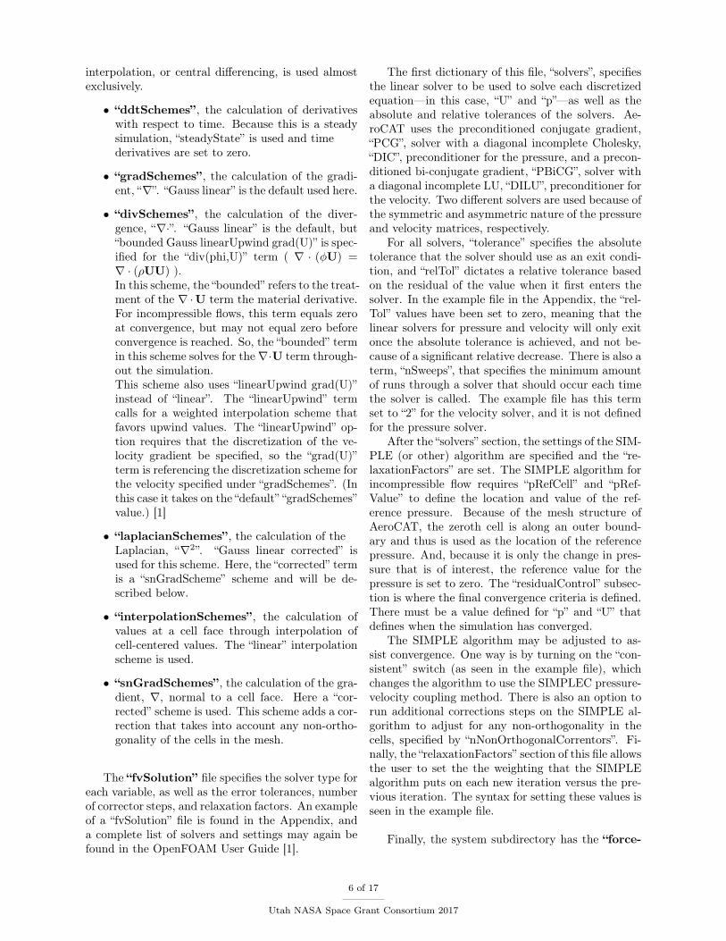
The SIMPLE algorithm may be adjusted to as-sist convergence. One way is by turning on the “con-sistent” switch (as seen in the example file), whichchanges the algorithm to use the SIMPLEC pressure-velocity coupling method. There is also an option torun additional corrections steps on the SIMPLE al-gorithm to adjust for any non-orthogonality in thecells, specified by “nNonOrthogonalCorrentors”. Fi-nally, the “relaxationFactors” section of this file allowsthe user to set the the weighting that the SIMPLEalgorithm puts on each new iteration versus the pre-vious iteration. The syntax for setting these values isseen in the example file.

Finally, the system subdirectory has the “force-

6 of 17

Utah NASA Space Grant Consortium 2017

CoeffsIncompressible” file (not shown in Figure 2)that contains the definitions of the lift and drag di-rections, the patches over which the forces should becalculated, and the reference values. As a note, someof the functions, like “residuals” mentioned above,do not require any additional information. But oth-ers, like “forceCoeffsIncompressible”, require that ad-ditional information be stored in the files similar tothis one in the “system” subdirectory. An example ofthe “forceCoeffsIncompressible” file is located in theAppendix.

II.C.2. Constant Subdirectory

The “constant” subdirectory contains a subdirectory,“polyMesh”, with the files defining the mesh, and pa-rameter files describing the flow. For the “simple-Foam” solver, the files “transportProperties” and “tur-bulenceProperties” are required.

The file “transportProperties” contains the singleline after its header:

nu [0 2 -1 0 0 0 0] 1e-6;

Where “nu” is the kinematic viscosity, ν, the brack-eted values describe the units of ν in base units (i.e.m2 · s−1), and the final number is the value of ν.Because AeroCAT is not meant to model turbulentflow, the file “turbulenceProperties” is simple as well,containing only two lines after the header:

transportModel Newtonian;simulationType laminar;

There are examples of both of these files in the Ap-pendix to provide an example of the header sections.

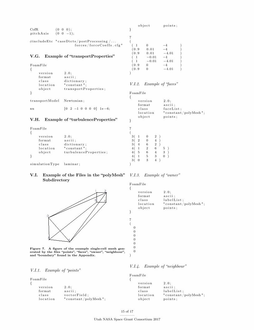
The “polyMesh” subdirectory contains five filesthat define the mesh: “points”, “faces”, “owner”, “neigh-bour”, and “boundary”. The Appendix contains anexample of each of these files for a mesh that, forsimplicity, has only one polyhedral cell (Figure 7).Of course, a more comprehensive description of themesh format may be found in the User Guide [1].

OpenFOAM meshes are unique in the fact thatthey do not require a prescribed cell shape. Eachcell is described by an arbitrary number of faces thatare each defined from an arbitrary number of points.Each face is part of two cells (or a boundary), andthus the cells are strung together through the defini-tion of which cell is the “owner” of a face and whichis the “neighbour” (or “boundary”). All of this infor-mation is contained in the files mentioned above anddescribed below.

The “points” file begins, after the header, withan integer announcing the number of points in themesh. This is followed by a list of x, y, z coordinatevalues enclosed in parenthesis. OpenFOAM assigns

numbered IDs to these points based on the order theyare found in this file, beginning with “0”.

The “faces” file also begins with an integer de-scribing the number of entries in the file. It is thenfollowed by a list of cell face descriptions that beginwith an integer telling the number of points used inthe face description followed by the list of the pointIDs that form the face. The order of the points isimportant, they must be ordered such that the facenormal vector is pointing out of the cell—from thecell with the lower numbered ID, the “owner”, intothe cell with the higher ID number, the “neighbour”.The normal is defined using the Right Hand Rule,such that if one were to be looking at the face frominside the owner cell, the points would be listed inthe clockwise direction.

As mentioned above, the “owner” file contains alist of the owner cells. As with the other files in thissubdirectory, this list begins by stating the numberof entries within. This number should be the sameas the number of faces that is declared in the “faces”file. Below that, the owner cell IDs are listed in theorder that corresponds to the order of the faces in the“faces” file. In the example in the Appendix, thereis only one cell, cell “0”, and thus it owns all sevenfaces. So, the example “owner” file has a “7” followedby a list of seven “0”s. As with the points, the cellnumbering begins with zero.

The “neighbour” file is similar to the “owner”file. It announces the number of entries, and then itcontains the list of neighbour cells listed in the ordercorresponding to the order of the faces in the “faces”file. There is a subtle difference with the “neighbour”file, however. For faces that form a boundary, thereis no neighbour cell, only an owner, so for these facesthe “neighbour” file may contain either a “-1”, or noentry at all. For the latter option, all boundary facesshould be listed last in the “faces” file. Thus, while the“faces” and “owner” files would have the same num-ber of entries, the “neighbour” file would contain thatnumber minus the number of boundary faces. Thepractice of listing all the boundary faces last is com-mon due to the way that boundaries are describedin OpenFOAM, as is described in the following para-graph.

The “boundary” file contains the definitions ofall the boundaries in the mesh. Below the header, thenumber of boundaries is stated followed by the list ofboundary descriptions. Each boundary descriptionbegins with a name to identify the boundary, followedby the “type” of boundary, the number of faces thatform that boundary (“nFaces”), and the ID of the facein the “faces” file where the list of that boundary’sfaces begins (“startFace”). It is necessary to list theboundary faces in the “faces” file such that all faces

7 of 17

Utah NASA Space Grant Consortium 2017

of a boundary are together. OpenFOAM recognizesa boundary by beginning at the face with ID “start-Face” and counts “nFaces” down the “faces” list. Thisis why it is common to include all boundary faces atthe end of the “faces” file.

The “boundary” file is not where boundary condi-tions are declared, but rather where boundary typesare assigned. The airfoil or wing boundary is a “wall”type, meaning it should be treated as a solid wall.Both the front and back outer boundaries are “patch”type boundaries, meaning they are flow inlets or out-lets. For three-dimensional simulation, the symmetryplane is declared a “symmetyPlane” type. In order torun a two-dimensional simulation in OpenFOAM, itis necessary to extrude the two-dimensional mesh to athickness of one cell and assign the original plane andthe new parallel plane to the “empty” type. Open-FOAM will then treat the simulation as a flow in twodimensions. Other boundary types not used by Ae-roCAT include “cyclic”, for repeated geometries, and“wedge”, for axi-symmetric flows [1].

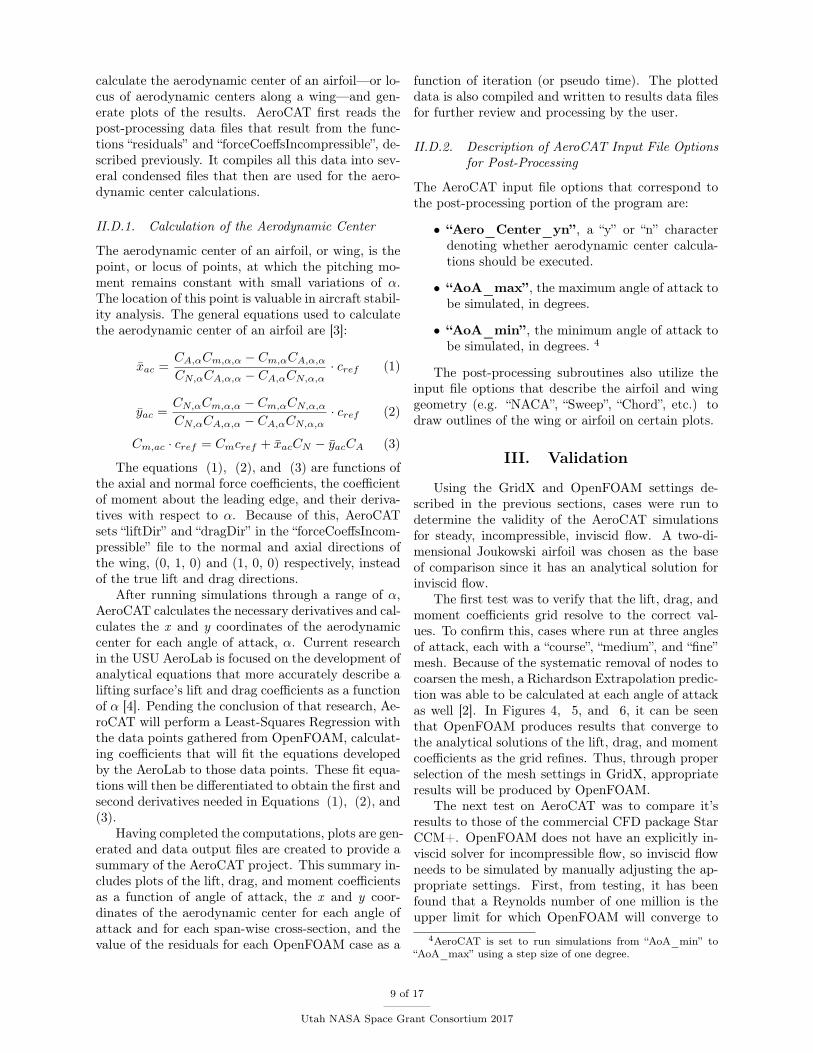
As stated above, one of the goals of AeroCAT isthe calculation of the locus of aerodynamic centersalong the span of a wing. To achieve this, the ringof boundary faces at each span-wise location alongthe wing is defined as a separate boundary. Thisallows each ring to be specified individually by thefunction “forceCoeffsIncompressible”, providing span-wise force distributions on the wing. This method ofboundary definition can be seen in Figure 3.

Figure 3. A view from above of a rectangular 3D wingdefined with each span-wise ring of boundary faces as aseparate boundary. Each shade of gray represents a differ-ent boundary patch with the endcap on the left and theroot on the right.

II.C.3. Time Subdirectories

The time subdirectories hold the start flow and bound-ary condition information for a case. They also storethe data output by OpenFOAM throughout the sim-ulation. For the cases run by AeroCAT, the initialconditions are saved in the “0” time directory, and theoutput results are stored in directories whose namecorresponds to the time/iteration for which the datawas calculated. For laminar “simpleFoam”, the Open-FOAM solver used by AeroCAT, the files “p” and “U”need to be found in the “0” subdirectory.

The “U” and “p” files found in the “0” subdirectoryinitialize the velocity and pressure of the flow and

assign conditions to each boundary. Following theheader, the file begins with a “dimensions” descrip-tion, which for velocity is “[0 1 -1 0 0 0 0]” (m1 · s−1)and for pressure is “[0 2 -2 0 0 0 0]” (m2 · s−2). Thisis followed by the term “internalField”, which is thedescription of what the flow inside the domain shouldinitialize as. To improve convergence for the steadyflow studied by AeroCAT, the entire internal flow isinitialized to the freestream velocity and to referencepressure. This is done by the term “uniform” followedby the x, y, z coordinate values of the desired velocityvector or by the scalar reference pressure value.

To set the boundary conditions in the “bound-aryField” entry, a list of the boundary names, de-fined in the “boundary” file, is given with a “type”for each. In the AeroCAT implementation, the frontand back boundaries are set to “freestream” for thevelocity and “freestreamPressure” for the pressure.These two boundary conditions calculate the flux ofthe flow through the boundary and, if the flow is intothe domain, the boundary holds a fixed velocity andpressure, but, if the flow is exiting the domain, theboundary enforces a zero-gradient condition for bothvelocity and pressure. For two-dimensional flow, Ae-roCAT sets the “type” for the airfoil to a “slip” con-dition to more accurately model inviscid flow and itsets the sides to an “empty” type, as discussed above.For three-dimensional flow, the wing and endcap areagain set as “slip” boundaries and the symmetry planeis of type “symmetry”. Examples of both the “U” and“p” files are located in the Appendix.

II.C.4. Description of AeroCAT Input File Optionsfor OpenFOAM

The AeroCAT input file options that correspond tothe OpenFOAM portion of the program are:

• “Convergence” , the value to be used in the“residualControl” section of the “fvSolution” file.It is the convergence criteria for the solver.

• “Sol_freq” , the value to be used for the “writeIn-terval” term in the “controlDict” file.

• “Velocity” , the magnitude of the freestreamvelocity, in meters per second.

As with GridX, “AoA_max” and “AoA_min” inthe AeroCAT input file dictate the range of angleof attack for which simulations will be run, so theyindirectly correspond to OpenFOAM input values.

II.D. Post-Processing

With the mesh generated and the simulation run, Ae-roCAT executes several post-processing routines to

8 of 17

Utah NASA Space Grant Consortium 2017

calculate the aerodynamic center of an airfoil—or lo-cus of aerodynamic centers along a wing—and gen-erate plots of the results. AeroCAT first reads thepost-processing data files that result from the func-tions “residuals” and “forceCoeffsIncompressible”, de-scribed previously. It compiles all this data into sev-eral condensed files that then are used for the aero-dynamic center calculations.

II.D.1. Calculation of the Aerodynamic Center

The aerodynamic center of an airfoil, or wing, is thepoint, or locus of points, at which the pitching mo-ment remains constant with small variations of α.The location of this point is valuable in aircraft stabil-ity analysis. The general equations used to calculatethe aerodynamic center of an airfoil are [3]:

xac =CA,αCm,α,α − Cm,αCA,α,αCN,αCA,α,α − CA,αCN,α,α

· cref (1)

yac =CN,αCm,α,α − Cm,αCN,α,αCN,αCA,α,α − CA,αCN,α,α

· cref (2)

Cm,ac · cref = Cmcref + xacCN − yacCA (3)

The equations (1), (2), and (3) are functions ofthe axial and normal force coefficients, the coefficientof moment about the leading edge, and their deriva-tives with respect to α. Because of this, AeroCATsets “liftDir” and “dragDir” in the “forceCoeffsIncom-pressible” file to the normal and axial directions ofthe wing, (0, 1, 0) and (1, 0, 0) respectively, insteadof the true lift and drag directions.

After running simulations through a range of α,AeroCAT calculates the necessary derivatives and cal-culates the x and y coordinates of the aerodynamiccenter for each angle of attack, α. Current researchin the USU AeroLab is focused on the development ofanalytical equations that more accurately describe alifting surface’s lift and drag coefficients as a functionof α [4]. Pending the conclusion of that research, Ae-roCAT will perform a Least-Squares Regression withthe data points gathered from OpenFOAM, calculat-ing coefficients that will fit the equations developedby the AeroLab to those data points. These fit equa-tions will then be differentiated to obtain the first andsecond derivatives needed in Equations (1), (2), and(3).

Having completed the computations, plots are gen-erated and data output files are created to provide asummary of the AeroCAT project. This summary in-cludes plots of the lift, drag, and moment coefficientsas a function of angle of attack, the x and y coor-dinates of the aerodynamic center for each angle ofattack and for each span-wise cross-section, and thevalue of the residuals for each OpenFOAM case as a

function of iteration (or pseudo time). The plotteddata is also compiled and written to results data filesfor further review and processing by the user.

II.D.2. Description of AeroCAT Input File Optionsfor Post-Processing

The AeroCAT input file options that correspond tothe post-processing portion of the program are:

• “Aero_Center_yn” , a “y” or “n” characterdenoting whether aerodynamic center calcula-tions should be executed.

• “AoA_max” , the maximum angle of attack tobe simulated, in degrees.

• “AoA_min” , the minimum angle of attack tobe simulated, in degrees. 4

The post-processing subroutines also utilize theinput file options that describe the airfoil and winggeometry (e.g. “NACA”, “Sweep”, “Chord”, etc.) todraw outlines of the wing or airfoil on certain plots.

III. Validation

Using the GridX and OpenFOAM settings de-scribed in the previous sections, cases were run todetermine the validity of the AeroCAT simulationsfor steady, incompressible, inviscid flow. A two-di-mensional Joukowski airfoil was chosen as the baseof comparison since it has an analytical solution forinviscid flow.

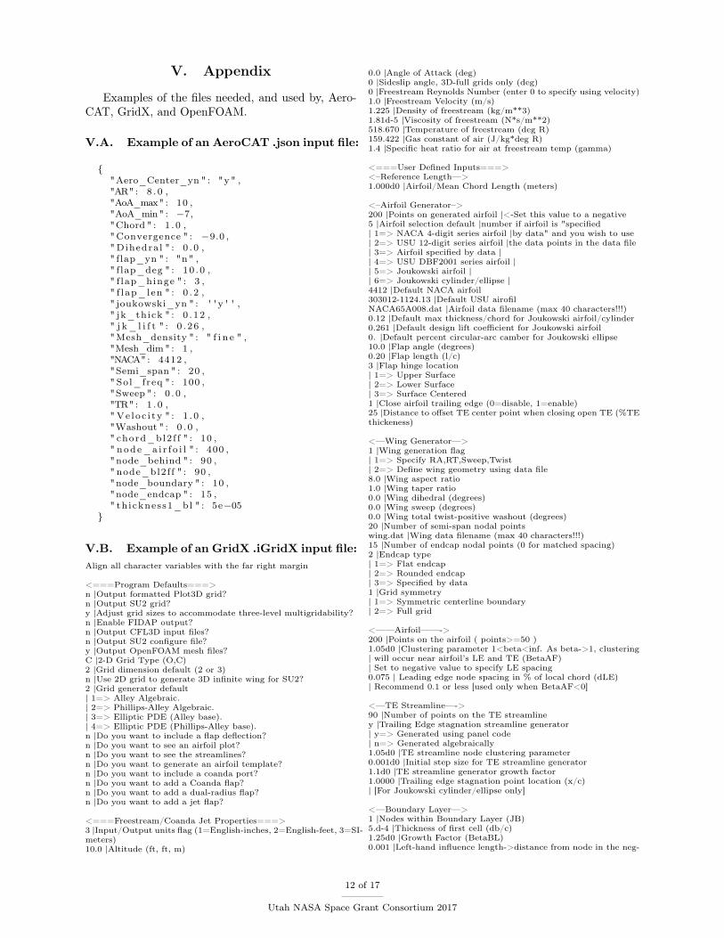
The first test was to verify that the lift, drag, andmoment coefficients grid resolve to the correct val-ues. To confirm this, cases where run at three anglesof attack, each with a “course”, “medium”, and “fine”mesh. Because of the systematic removal of nodes tocoarsen the mesh, a Richardson Extrapolation predic-tion was able to be calculated at each angle of attackas well [2]. In Figures 4, 5, and 6, it can be seenthat OpenFOAM produces results that converge tothe analytical solutions of the lift, drag, and momentcoefficients as the grid refines. Thus, through properselection of the mesh settings in GridX, appropriateresults will be produced by OpenFOAM.

The next test on AeroCAT was to compare it’sresults to those of the commercial CFD package StarCCM+. OpenFOAM does not have an explicitly in-viscid solver for incompressible flow, so inviscid flowneeds to be simulated by manually adjusting the ap-propriate settings. First, from testing, it has beenfound that a Reynolds number of one million is theupper limit for which OpenFOAM will converge to

4AeroCAT is set to run simulations from “AoA_min” to“AoA_max” using a step size of one degree.

9 of 17

Utah NASA Space Grant Consortium 2017

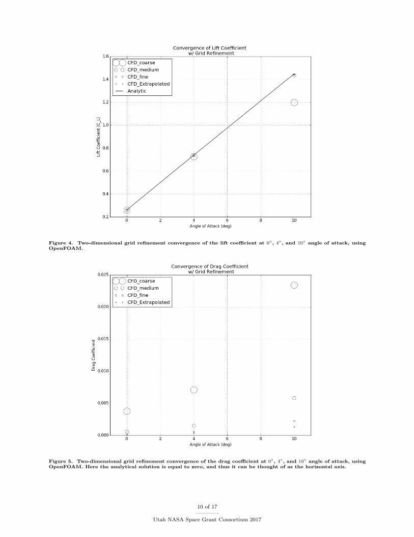
Figure 4. Two-dimensional grid refinement convergence of the lift coefficient at 0◦, 4◦, and 10◦ angle of attack, usingOpenFOAM.

Figure 5. Two-dimensional grid refinement convergence of the drag coefficient at 0◦, 4◦, and 10◦ angle of attack, usingOpenFOAM. Here the analytical solution is equal to zero, and thus it can be thought of as the horizontal axis.

10 of 17

Utah NASA Space Grant Consortium 2017

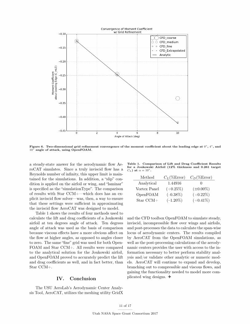
Figure 6. Two-dimensional grid refinement convergence of the moment coefficient about the leading edge at 0◦, 4◦, and10◦ angle of attack, using OpenFOAM.

a steady-state answer for the aerodynamic flow Ae-roCAT simulates. Since a truly inviscid flow has aReynolds number of infinity, this upper limit is main-tained for the simulations. In addition, a “slip” con-dition is applied on the airfoil or wing, and “laminar”is specified as the “simulationType”. The comparisonof results with Star CCM+—which does has an ex-plicit inviscid flow solver—was, then, a way to ensurethat these settings were sufficient in approximatingthe inviscid flow AeroCAT was designed to model.

Table 1 shows the results of four methods used tocalculate the lift and drag coefficients of a Joukowskiairfoil at ten degrees angle of attack. Ten degreesangle of attack was used as the basis of comparisonbecause viscous effects have a more obvious affect onthe flow at higher angles, as opposed to angles closerto zero. The same “fine” grid was used for both Open-FOAM and Star CCM+. All results were comparedto the analytical solution for the Joukowski airfoil,and OpenFOAM proved to accurately predict the liftand drag coefficients as well, and in fact better, thanStar CCM+.

IV. Conclusion

The USU AeroLab’s Aerodynamic Center Analy-sis Tool, AeroCAT, utilizes the meshing utility GridX

Table 1. Comparison of Lift and Drag Coefficient Resultsfor a Joukowski Airfoil (12% thickness and 0.261 targetCL) at α = 10◦.

Method CL(%Error) CD(%Error)Analytical 1.44916 0

Vortex Panel (+0.25%) (±0.00%)OpenFOAM (–0.38%) (+0.22%)Star CCM+ (–1.20%) (+0.41%)

and the CFD toolbox OpenFOAM to simulate steady,inviscid, incompressible flow over wings and airfoils,and post-processes the data to calculate the span-wiselocus of aerodynamic centers. The results compiledby AeroCAT from the OpenFOAM simulations, aswell as the post-processing calculations of the aerody-namic centers provides the user with access to the in-formation necessary to better perform stability anal-ysis and/or validate other analytic or numeric mod-els. AeroCAT will continue to expand and develop,branching out to compressible and viscous flows, andgaining the functionality needed to model more com-plicated wing designs. (

11 of 17

Utah NASA Space Grant Consortium 2017

V. Appendix

Examples of the files needed, and used by, Aero-CAT, GridX, and OpenFOAM.

V.A. Example of an AeroCAT .json input file:

{"Aero_Center_yn " : "y" ,"AR" : 8 . 0 ,"AoA_max" : 10 ,"AoA_min" : −7,"Chord " : 1 . 0 ,"Convergence " : −9.0 ,"Dihedra l " : 0 . 0 ," flap_yn " : "n" ," f lap_deg " : 10 . 0 ," f lap_hinge " : 3 ," f lap_len " : 0 . 2 ," joukowski_yn " : ' 'y ' ' ," jk_thick " : 0 . 12 ," j k_ l i f t " : 0 . 26 ,"Mesh_density " : " f i n e " ,"Mesh_dim" : 1 ,"NACA" : 4412 ,"Semi_span " : 20 ," Sol_freq " : 100 ,"Sweep " : 0 . 0 ,"TR" : 1 . 0 ," Ve loc i ty " : 1 . 0 ,"Washout " : 0 . 0 ," chord_bl2 f f " : 10 ," node_a i r f o i l " : 400 ,"node_behind " : 90 ," node_bl2f f " : 90 ,"node_boundary " : 10 ,"node_endcap " : 15 ," th ickness1_bl " : 5e−05

}

V.B. Example of an GridX .iGridX input file:Align all character variables with the far right margin

<===Program Defaults===>n |Output formatted Plot3D grid?n |Output SU2 grid?y |Adjust grid sizes to accommodate three-level multigridability?n |Enable FIDAP output?n |Output CFL3D input files?n |Output SU2 configure file?y |Output OpenFOAM mesh files?C |2-D Grid Type (O,C)2 |Grid dimension default (2 or 3)n |Use 2D grid to generate 3D infinite wing for SU2?2 |Grid generator default| 1=> Alley Algebraic.| 2=> Phillips-Alley Algebraic.| 3=> Elliptic PDE (Alley base).| 4=> Elliptic PDE (Phillips-Alley base).n |Do you want to include a flap deflection?n |Do you want to see an airfoil plot?n |Do you want to see the streamlines?n |Do you want to generate an airfoil template?n |Do you want to include a coanda port?n |Do you want to add a Coanda flap?n |Do you want to add a dual-radius flap?n |Do you want to add a jet flap?

<===Freestream/Coanda Jet Properties===>3 |Input/Output units flag (1=English-inches, 2=English-feet, 3=SI-meters)10.0 |Altitude (ft, ft, m)

0.0 |Angle of Attack (deg)0 |Sideslip angle, 3D-full grids only (deg)0 |Freestream Reynolds Number (enter 0 to specify using velocity)1.0 |Freestream Velocity (m/s)1.225 |Density of freestream (kg/m**3)1.81d-5 |Viscosity of freestream (N*s/m**2)518.670 |Temperature of freestream (deg R)159.422 |Gas constant of air (J/kg*deg R)1.4 |Specific heat ratio for air at freestream temp (gamma)

<===User Defined Inputs===><–Reference Length—>1.000d0 |Airfoil/Mean Chord Length (meters)

<–Airfoil Generator–>200 |Points on generated airfoil |<-Set this value to a negative5 |Airfoil selection default |number if airfoil is "specified| 1=> NACA 4-digit series airfoil |by data" and you wish to use| 2=> USU 12-digit series airfoil |the data points in the data file| 3=> Airfoil specified by data || 4=> USU DBF2001 series airfoil || 5=> Joukowski airfoil || 6=> Joukowski cylinder/ellipse |4412 |Default NACA airfoil303012-1124.13 |Default USU airofilNACA65A008.dat |Airfoil data filename (max 40 characters!!!)0.12 |Default max thickness/chord for Joukowski airfoil/cylinder0.261 |Default design lift coefficient for Joukowski airfoil0. |Default percent circular-arc camber for Joukowski ellipse10.0 |Flap angle (degrees)0.20 |Flap length (l/c)3 |Flap hinge location| 1=> Upper Surface| 2=> Lower Surface| 3=> Surface Centered1 |Close airfoil trailing edge (0=disable, 1=enable)25 |Distance to offset TE center point when closing open TE (%TEthickeness)

<—Wing Generator—>1 |Wing generation flag| 1=> Specify RA,RT,Sweep,Twist| 2=> Define wing geometry using data file8.0 |Wing aspect ratio1.0 |Wing taper ratio0.0 |Wing dihedral (degrees)0.0 |Wing sweep (degrees)0.0 |Wing total twist-positive washout (degrees)20 |Number of semi-span nodal pointswing.dat |Wing data filename (max 40 characters!!!)15 |Number of endcap nodal points (0 for matched spacing)2 |Endcap type| 1=> Flat endcap| 2=> Rounded endcap| 3=> Specified by data1 |Grid symmetry| 1=> Symmetric centerline boundary| 2=> Full grid

<——Airfoil——->200 |Points on the airfoil ( points>=50 )1.05d0 |Clustering parameter 1<beta<inf. As beta->1, clustering| will occur near airfoil’s LE and TE (BetaAF)| Set to negative value to specify LE spacing0.075 | Leading edge node spacing in % of local chord (dLE)| Recommend 0.1 or less [used only when BetaAF<0]

<—TE Streamline—->90 |Number of points on the TE streamliney |Trailing Edge stagnation streamline generator| y=> Generated using panel code| n=> Generated algebraically1.05d0 |TE streamline node clustering parameter0.001d0 |Initial step size for TE streamline generator1.1d0 |TE streamline generator growth factor1.0000 |Trailing edge stagnation point location (x/c)| [For Joukowski cylinder/ellipse only]

<—Boundary Layer—>1 |Nodes within Boundary Layer (JB)5.d-4 |Thickness of first cell (db/c)1.25d0 |Growth Factor (BetaBL)0.001 |Left-hand influence length->distance from node in the neg-

12 of 17

Utah NASA Space Grant Consortium 2017

ative| i-direction that is used to define the surface normal (dZL/c)0.001 |Right-hand influence length->distance from node in the pos-tive| i-direction that is used to define the surface normal (dZR/c)|Boundary Layer influence lengths are equal to the jet size (tj/c)| for O-grids containing Coanda jets (dZL=dZR=tj)|If boundary layer nodes are crossing, reduce JB,db,or BetaBL,| or increase dZL and dZR. Increasing dZL and dZR might cause| boundary-layer cells to become skewed. Reducing dZL and dZR| will force the boundary to be orthogonal to the surface but| increases the chance of crossed nodes.n |Expand trailing boundary layer?5.0e-3 |Thickness of the j=1 boundary layer cells at i=1 and i=IM(dEBL)1.1d0 |Growth factor of the boundary layer cells at i=1 and i=IM(BetaEBL)15 |Number of nodes past trailing edge where expansion begins(EBLs)

<—–Inner Grid/Outer Boundary—–>90 |Nodes between the outer boundary| and the boundary layer (JIG)10 |Number of chord lengths to outer boundary (I_chord)0. |Angle that outer boundary O-grid joint line is rotated from|horizontal (degrees)1.25d0 |Transition growth factor for Phillips-Alley method (Tgf>0)| Larger values of Tgf will increase the occurrence of folded nodes| but will cause the grid to be more orthogonal to the surface| The "transition" region is where the grid changes direction| from orthogonal to the airfoil surface to a straight line| toward the outer boundary.0.001d0 |Clustering parameter 0<beta<inf, as beta->inf| boundary node clustering will occur near the| leading edge of the boundary| NOTE: For Joukowski Cylinders, 1<beta<inf, as beta->1| boundary node clustering will occur near the ends| (i=1 and IM) of the boundary (BetaOB)1 |match_IG=1 will match the first row width of the algebraic| inner grid to the last row in the boundary layer1.06 |Clustering parameter 1<beta<inf, as beta->1 algebraic innernode| clustering will occur near the airfoil: for match_IG=0 only (Be-taIG)

<—-Elliptic PDE—->0.20d0 |Forcing Parameter (FPO>0) as FPO->0 orthogonality isforced.0.20d0 |Forcing Parameter (FPC>0) as FPC->0 clustering nearairfoil is forced.0.1d0 |Relaxation factor (lambda)0.08d0 |Relaxation factor (wp)0.08d0 |Relaxation factor (wq)1.d-3 |Convergance Criteria (total x-y error < conv)100 |Maximum number of allowable iterations

<—-Output Files—->jk_0 |Output filename w/o extension (leave blank to use .GENfilename).FDNEUT ==>FIDAP grid output.p3D ==>Formatted Plot3D grid output.unf ==>Unformatted Plot3D grid output.oGridX ==>Name of elliptic-inner-grid file that can be used inOuterGrid.exe.inp ==>CFL3D input file

<——CFL3D/SU2/OpenFOAM Inputs——>5. |Steady CFL Number (Default=5)-99. |Moment center in X direction,positive back (Set to -99 tocompute at root 1/4-chord) (m)0. |Moment center in Y direction,positive up (m)0. |Moment center in Z direction,positive out left wing (m)-99. |Reference area (Set to -99 to for grid dimensions)-99. |Lateral reference length (Set to -99 to for grid dimensions)-99. |Longitudinal reference length (Set to -99 to for grid dimen-sions)1000 |Number of fine-grid iterations1000 |Number of medium-grid iterations1000 |Number of coarse-grid iterations1000 |Number of coarsest-grid iterationsfine |SU2/OpenFOAM mesh density (fine, medium, coarse)-6 |SU2/OpenFOAM residual convergence criteria10 |Frequency of SU2/OpenFOAM solution files

<——Coanda Jet Grid——>0.85d0 |Coanda port location from leading edge (x/c)0.00125d0 |Coanda port thickness (t/c)0.95 |Airfoil chord length with dual-radius flap0.4 |Blowing momentum coefficient (Cmu)518.670 |Jet stagnation temperature (deg R)20 |Nodes within Jet Layer (JJ)1.d-5 |Thickness of first cell (dj/c)0 |Nodes aft of coanda port (0 for auto spacing)1 |match_J=1 will match the node clustering on the| airfoil aft of the jet to the clustering in| front the jet2.55d0 |Clustering parameter 1<beta<inf, as beta->1| clustering will occur near the jet and the| TE: for match_J=0 only (BetaJ)

<——Jet Flap Grid——>1.d-5 |Thickness of first cell (djf/c)| NOTE: It is recommended that the thickness of the first| cell in the boundary layer, "db", and "djf" be equal100 |Number of nodes along fore-lower airfoil boundary, betweenleading edge and upper duct inlet (Iafl)160 |Number of nodes along mid-lower airfoil boundary, betweenupper and lower duct inlets (Iaml)160 |Number of nodes along aft-lower airfoil boundary, betweentraling edge of lower jet flap and lower duct inlet (Iaal)-20 |Number of nodes along upper surface of airfoil, between lead-ing edge and trailing edge of upper jet flap (Iatu)| Set to a negative value to equal the total number of nodes alongthe lower surface15. |Thrust vector angle, positive down (degrees)0.63042 |Axial location of upper jet flap hinge (xjfu/c)0.63042 |Axial location of lower jet flap hinge (xjfl/c)0.00800 |Jet flap airfoil wall thickness (twj/c)0.07948 |Ejector (exit) nozzle height (tej/c)0.02323 |Inner nozzle throat height (ttj/c)0.03843 |Inner nozzle total height, includes inner nozzle wall thick-ness (tnj/c)100 |Number of axial nodes within nozzle (Inoz)40 |Number of radial nodes in the inner nozzle throat (Jint)20 |Number of radial nodes in the inner nozzle walls (Jinw)0.01412 |Upper bypass inlet height (tubi/c)0.01782 |Upper bypass duct height (tubd/c)100 |Number of axial nodes within the upper bypass duct (Iubd)40 |Number of radial nodes within the upper bypass duct (Jubd)0.01225 |Lower bypass inlet height (tlbi/c)0.01552 |Lower bypass duct height (tlbd/c)60 |Number of axial nodes within the lower bypass duct (Ilbd)40 |Number of radial nodes within the lower bypass duct (Jlbd)

<—-OuterGrid Generator—-> (For 3-D Joukowski cylinders only)40 |Number of chords from airfoil to outer boudary (I_ochord)16 |Number of additional wake nodes (jadd)16 |Number of additional radial nodes (kadd)

V.C. Example of “controlDict”

FoamFile{

ve r s i on 2 . 0 ;format a s c i i ;c l a s s d i c t i ona ry ;l o c a t i o n " system " ;ob j e c t c on t r o lD i c t ;

}

app l i c a t i on simpleFoam ;

startFrom startTime ;

startTime 0 ;

stopAt endTime ;

endTime 300 ;

13 of 17

Utah NASA Space Grant Consortium 2017

deltaT 0 . 1 ;

wr i t eContro l runTime ;

w r i t e I n t e r v a l 10 ;

purgeWrite 0 ;

writeFormat a s c i i ;

w r i t eP r e c i s i o n 6 ;

writeCompress ion o f f ;

timeFormat gene ra l ;

t imePrec i s i on 6 ;

runTimeModif iable t rue ;

f un c t i on s{#includeFunc r e s i d u a l s#includeFunc f o r c eCoe f f s I n c ompr e s s i b l e}

V.D. Example of “fvSchemes”

FoamFile{

ve r s i on 2 . 0 ;format a s c i i ;c l a s s d i c t i ona ry ;l o c a t i o n " system " ;ob j e c t fvSchemes ;

}

ddtSchemes{d e f au l t s t eadyState ;

}

gradSchemes{d e f au l t Gauss l i n e a r ;

}

divSchemes{d e f au l t Gauss l i n e a r ;d iv ( phi ,U) bounded Gauss l inearUpwind grad (U) ;

}

lap lac ianSchemes{d e f au l t Gauss l i n e a r co r r e c t ed ;

}

in te rpo la t i onSchemes{d e f au l t l i n e a r ;

}

snGradSchemes{d e f au l t c o r r e c t ed ;

}

V.E. Example of “fvSolution”

FoamFile{

ve r s i on 2 . 0 ;format a s c i i ;c l a s s d i c t i ona ry ;l o c a t i o n " system " ;ob j e c t f vSo l u t i on ;

}

s o l v e r s{

p{

s o l v e r PCG;p r e cond i t i on e r DICto l e r an c e 1e−06;r e lTo l 0 ;

}

U{

s o l v e r PBiCG;p r e cond i t i on e r DILUnSweeps 2 ;t o l e r an c e 1e−08;r e lTo l 0 ;

}

}

SIMPLE{

nNonOrthogonalCorrectors 0 ;pRefCel l 0 ;pRefValue 0 ;

c on s i s t e n t yes ;

r e s i dua lCon t r o l{

p 1e−6;U 1e−6;

}}

r e l axa t i onFac t o r s{

f i e l d s{

p 0 . 3 ;}equat ions{

U 0 . 7 ;}

}

V.F. Example of “forceCoeffsIncompressible”

patches ( a i r f o i l ) ;

magUInf 1 ;lRe f 1 ;Aref . 1 ;

l i f t D i r (0 1 0 ) ;dragDir (1 0 0 ) ;

14 of 17

Utah NASA Space Grant Consortium 2017

CofR (0 0 0 ) ;p i tchAxis (0 0 −1);

#inc ludeEtc " ca s eD i c t s / pos tProce s s ing / . . .f o r c e s / f o r c eCo e f f s . c f g "

V.G. Example of “transportProperties”

FoamFile{

ve r s i on 2 . 0 ;format a s c i i ;c l a s s d i c t i ona ry ;l o c a t i o n " constant " ;ob j e c t t r an spo r tP rope r t i e s ;

}

transportModel Newtonian ;

nu [ 0 2 −1 0 0 0 0 ] 1e−6;

V.H. Example of “turbulenceProperties”

FoamFile{

ve r s i on 2 . 0 ;format a s c i i ;c l a s s d i c t i ona ry ;l o c a t i o n " constant " ;ob j e c t tu rbu l enc ePrope r t i e s ;

}

s imulat ionType laminar ;

V.I. Example of the Files in the “polyMesh”Subdirectory

Figure 7. A figure of the example single-cell mesh gen-erated by the files “points”, “faces”, “owner”, “neighbour”,and “boundary” found in the Appendix.

V.I.1. Example of “points”

FoamFile{

ve r s i on 2 . 0 ;format a s c i i ;c l a s s v e c t o rF i e l d ;l o c a t i o n " constant /polyMesh " ;

ob j e c t po in t s ;}

7(( 1 0 −4 )( 0 . 9 0 .01 −4 )( 0 . 9 0 .01 −4.01 )( 1 −0.01 −4 )( 1 −0.01 −4.01 )( 0 . 9 0 −4 )( 0 . 9 0 −4.01 )

)

V.I.2. Example of “faces”

FoamFile{

ve r s i on 2 . 0 ;format a s c i i ;c l a s s f a c eL i s t ;l o c a t i o n " constant /polyMesh " ;ob j e c t po in t s ;

}

7(3( 1 0 2 )3( 2 0 4 )3( 4 6 2 )4( 1 2 6 5 )4( 5 6 4 3 )4( 1 5 3 0 )3( 0 3 4 )

)

V.I.3. Example of “owner”

FoamFile{

ve r s i on 2 . 0 ;format a s c i i ;c l a s s l a b e l L i s t ;l o c a t i o n " constant /polyMesh " ;ob j e c t po in t s ;

}

7(

0000000

)

V.I.4. Example of “neighbour”

FoamFile{

ve r s i on 2 . 0 ;format a s c i i ;c l a s s l a b e l L i s t ;l o c a t i o n " constant /polyMesh " ;ob j e c t po in t s ;

15 of 17

Utah NASA Space Grant Consortium 2017

}

7(

−1−1−1−1−1−1−1

)

V.I.5. Example of “boundary”

FoamFile{

ve r s i on 2 . 0 ;format a s c i i ;c l a s s polyBoundaryMesh ;l o c a t i o n " constant /polyMesh " ;ob j e c t po in t s ;

}

6(

top{

type empty ;nFaces 1 ;s ta r tFace 0 ;

}

r i g h t{

type wal l ;nFaces 2 ;s ta r tFace 1 ;

}

f r on t{

type patch ;nFaces 1 ;s ta r tFace 3 ;

}

bottom{

type empty ;nFaces 1 ;s ta r tFace 4 ;

}

l e f t{

type symmetryPlane ;nFaces 1 ;s ta r tFace 5 ;

}

back{

type patch ;nFaces 1 ;s ta r tFace 6 ;

})

V.J. Example of “U” from Time Subdirec-tory “0”

FoamFile{

ve r s i on 2 . 0 ;format a s c i i ;c l a s s vo lVec to rF i e ld ;ob j e c t U;

}

dimensions [ 0 1 −1 0 0 0 0 ] ;

i n t e r n a l F i e l d uniform (1 0 0 ) ;

boundaryField{

back{

type f r e e s t r eam ;f rees t reamValue uniform (1 0 0 ) ;

}

f r on t{

type f r e e s t r eam ;f rees t reamValue uniform (1 0 0 ) ;

}

a i r f o i l{

type s l i p ;}

s i d e s{

type empty ;}

}

V.K. Example of “p” from Time Subdirec-tory “0”

FoamFile{

ve r s i on 2 . 0 ;format a s c i i ;c l a s s v o l S c a l a rF i e l d ;ob j e c t p ;

}

dimensions [ 0 2 −2 0 0 0 0 ] ;

i n t e r n a l F i e l d uniform 0 ;

boundaryField{

back{

type f r e e s t r eamPre s su r e ;}

f r on t{

type f r e e s t r eamPre s su r e ;}

a i r f o i l

16 of 17

Utah NASA Space Grant Consortium 2017

{type zeroGradient ;

}

s i d e s{

type empty ;}

}

Acknowledgments

The author is extremely grateful to his fellow studentsin the USU AeroLab for sharing their knowledge and sug-gestions.

References

[1] OpenFOAM Ltd. User guide.http://www.openfoam.com/documentation/user-guide/, April 2017.

[2] Warren F. Phillips. Minimizing induced drag withwing twist, computational-fluid-dynamics validation.Journal of Aircraft, 43(2), March-April 2006.

[3] Warren F. Phillips. Mechanics of Flight. John Wiley& Sons, Inc., 2nd edition, 2010.

[4] Orrin D. Pope. The aerodynamic center of inviscidairfoils. In Utah NASA Space Grant Consortium Fel-lowship Symposium, 2017.

17 of 17

Utah NASA Space Grant Consortium 2017