CAV03-GS-12-002 Fifth International Symposium on Cavitation (CAV2003)Osaka, Japan, November 1–4, 2003

A VISCOUS/INVISCID COUPLED FORMULATIONFOR UNSTEADY SHEET CAVITATION MODELLING OF MARINE PROPELLERS

Francesco SalvatoreINSEAN, Italian Ship Model Basin

f.salvatore@insean.it

Claudio TestaINSEAN, Italian Ship Model Basin

c.testa@insean.it

Luca GrecoINSEAN, Italian Ship Model Basin

l.greco@insean.it

ABSTRACT

The theoretical modelling of marine propeller cavitation is ad-dressed. The objective is to develop an enhanced inviscid–flowmethodology to be integrated into a hybrid viscous/inviscid ap-proach for the analysis and design of marine propulsors at modelscale. The proposed methodology is based on a nonlinear bound-ary integral formulation that includes trailing vorticity analysis,boundary layer solution and sheet cavitation modelling. The the-oretical approach is described with emphasis on the procedureto combine models into an integrated boundary element method.Numerical results by the proposed methodology are presented inorder to verify the numerical scheme and to validate propellerflow and cavitation pattern predictions against experimental data.

INTRODUCTION

The present paper addresses the development of design–orientedcomputational tools for marine propeller cavitation modelling atmodel scale.

State–of–the–art theoretical models allow to describe complexcavitating flows where the evolution (inception, development andcollapse) of a water/vapour mixtures is strongly affected by flowturbulence and vorticity, fluid surface tension and viscosity. Theo-retical methods capable to attack such kind of problems are basedon the Navier–Stokes equations for viscous flows. Numericalmethods mostly include Reynolds Averaged Navier–Stokes Equa-tion (RANSE) models, and, at an early development stage, largeEddy Simulation (LES) models.

Recent literature on the subject demonstrates the capability ofthese models to address cavitation on simple two–dimensionaland three–dimensional problems. It is also apparent the strongeffort to extend these models to the analysis of marine propellerflows. For this type of flows, difficulties related to the compu-tational grid quality and size, the coupling of fixed and rotatingframes of reference, represent classical drawbacks to the applica-tion of viscous–flow methods in a design context.

Nevertheless, fluid–dynamics models based on the simplifying

assumption that the flow is inviscid have been successfully usedfor decades (see, eg., for cavitating flows [1] and[2]) and are cur-rently largely applied at design level of propeller–based propul-sors. The limits of these models are related to the fact that theyare not able to take into account most of rotational and viscousflow effects In spite of that, their success is largely due to the fa-vorable ratio between accuracy of predictions and computationalcosts.

In order to exploit the advantages of inviscid–flow and viscous–flow methodologies, in the last few years an increasing interest isbeing posed to numerical tools that combine the two approachesto address practical problems where the propeller is consideredin its actual environment, and hence including fixed interactingbodies. Maybe the first applications of suchhybrid approachare related to the analysis of non–cavitating pump flow and tur-bomachinery. Recent marine applications cover hull/propeller,propeller/rudder, propeller/pod/strut. Typically, the flowfieldaround the rotating components (propeller blades) is analysedby inviscid–flow approaches, whereas the flow around the fixedcomponents is studied by means of viscous–flow solvers. Variousinviscid-flow/viscous–flow coupling techniques are possible.

In the present paper, the development of inviscid–flow solversto be integrated into a hybrid approach for the analysis of cavita-tion on marine propulsors components at model scale is consid-ered. Two issues are emphasized here:(i) to enhance the accu-racy of the inviscid–flow solver by including the modelling of thepropeller–induced vortical wake and the modelling of the viscos-ity effects into the boundary layer, and(ii) to assess the capabilityof such an enhanced inviscid–flow solver to address the hydrody-namics of cavitating propellers through validation against experi-mental data.

The proposed theoretical model is based on a boundary integralformulation for the analysis of ’quasi–potential’ flows, i.e., in-viscid irrotational flows around lifting/thrusting bodies. The term’quasi–potential’ is used to denote a mathematical model in whichthe flow is potential everywhere except for a zero thickness layerwhere the vorticity related to the lift/thrust generation mechanismis shed downstream the body. This surface is labelled as the trail-

1

ing wake, and represents a discountinuity surface for the velocitypotential.

The case of interest here is an isolated propeller in a prescribednon–uniform upstream flow that simulates the ship hull flow in-coming to the propeller disk. Blade flow conditions are character-ized by high Reynolds number and the advance coefficient is closeto the design value. Under these circumstances viscosity effectsare confined into a thin rotational region attached to the body sur-face and surrounding the vortical wake, and hence boundary layerassumptions are adequate to address the problem.

Outside the viscous vortical region, it is assumed that thepropeller–induced perturbation velocity is irrotational and henceit may be represented in terms of a scalar potential asv = ∇ϕ.The assumption above is valid in the case of uniform upstreamflow, whereas for non–uniform inflow it is approximated in thelimit as the turbulent upstream flow does not strongly interact withthe propeller turbulent boundary layer.

Trailing wake modelling and viscous vortical layer analysis arecoupled with a cavitation model that is valid to study sheet cavi-ties that form in the leading edge region of the propeller blades, inboth uniform and non–uniform flow conditions. The cavity trail-ing edge is supposed to be stable and hence cloud cavitation is notaddressed.

In the following sections, the theoretical model and the inte-gration approach are explained in detail. Next, numerical resultsby the proposed approach are presented in order to verify bothnumerical scheme convergence and consistency and to validatepredictions against experimental data.

THEORETICAL FORMULATION

Non–cavitating, quasi–potential flow

Consider a frame of reference fixed to the propeller with thex-axis parallel to the propeller axis and downstream pointing. Theincoming flow to the propeller has a velocityv

I= v

A+ Ω×x,

wherevA

is the upstream flow, andΩ is the angular velocity ofthe propeller. The total velocity field in the propeller frame ofreference is

q = vI

+ ∇ϕ. (1)

The present derivation is valid for a non uniformvI

field.Assuming that the flow is incompressible, the continuity equa-

tion reduces to the Laplace equation∇2ϕ = 0. A classical ap-proach based on the third Green identity yields for an arbitrarypointx immersed into the fluid

ϕ(x) =∮S

B

(∂ϕ

∂nG− ϕ

∂G

∂n

)dS(y)

+∫S

W

[∆

(∂ϕ

∂n

)G−∆ϕ

∂G

∂n

]dS(y), (2)

whereSB

denotes the body surface,SW

the trailing wake surface,andn is the unit normal. The symbol∆ denotes discontinuityacross the wake surface, andG = −1/4π‖x − y‖ is the unitsource in the unbounded three–dimensional space.

The pressurep is given by Bernoulli’s theorem that, in the frameof reference fixed to the propeller, reads

∂ϕ

∂t+

12q2 +

p

ρ+ gz0 =

12v2

I+

p0

ρ, (3)

whereq = ‖q‖, vI

= ‖vI‖, whereasg is the gravity acceleration

andz0 denotes depth.In the limit asx tends to the body surface, Equation (2) pro-

vides a boundary integral equation forϕ to be solved with suitableboundary conditions.

Consider first inviscid, non cavitating flow conditions. On thebody surface the impermeability condition yieldsq · n = 0, or,recalling Eq. (1),

∂ϕ

∂n= −v

I· n on S

B. (4)

Across the trailing wake surface, mass and momentum conserva-tion laws are imposed to obtain that both pressure and the normalcomponent of the perturbation velocity∂ϕ/∂n are continuous

∆p = 0; ∆(

∂ϕ

∂n

)= 0; on S

W. (5)

Combining the Bernoulli Eq. (3) and∆p = 0, one obtaines that∆ϕ is constant following wake particles

∆ϕ (x, t) = ∆ϕ (xT E

, t− τ) on SW

, (6)

wherexT E

is a wake point at the blade trailing edge andτ is theconvection time between wake pointsx andx

T E. A further con-

dition on ϕ is required in order to assure that no finite pressurejump may exist at the body trailing edge (Kutta condition) In thepresent approach, this corresponds to impose that∆ϕ at the trail-ing edge equals the difference between potentials at the two sidesof the body surface [3].

For further reference, an arbitrary curvilinear coordinate sys-tem(ξ, η) is introduced on each body and trailing wake surfaces.Specifically,ξ is directed along the blade in the chordwise direc-tion and in streamwise direction on the wake, withξ = 0 denotingthe blade leading edge, whereasη is directed in the spanwise di-rection on the blade and in the radial direction on the wake. Unitvectorseξ, eη represent the covariant base associated to the(ξ, η)coordinate system.

Trailing wake alignment

The location of the wake surface in Eq. (2) is not knowna pri-ori and may be either prescribed or determined as a part of theflowfield solution. The latter approach is considered here.

A physically–consistent wake shape is determined by recallingthat the trailing wake represents a vortical layer formed by all theparticles that came in contact with the body. Hence it must bealigned to the local flowfield. The procedure is labelled aswakealignmentand is achieved in two phases. First, the perturbationvelocity field in the wake region is computed by using a boundaryintegral representation for the velocity potential. This is obtained

2

by taking the gradient of Eq. (2), to obtain∇ϕ at any point on thewake surface.

∇xϕ(x, t) =∮S

B

[∂ϕ

∂n∇xG− ϕ∇x

(∂G

∂n

)]dS(y) (7)

+∫S

W

[∆

(∂ϕ

∂n

)∇xG − ∆ϕ∇x

(∂G

∂n

)]dS(y),

where the symbol∇x denotes the gradient operator acting onx.Next, wake points are moved by imposing thatS

Wmust be tan-

gent to the local velocity fieldq = ∇ϕ + vI. The alignment

procedure of an arbitrary wake pointxW

is then accomplished bya Lagrangian–type approach as

xW

(τ + ∆τ) = xW

(τ) +∫ τ+∆τ

τ

[∇ϕ (xW

, τ) + vI] dτ. (8)

whereτ denotes the convection time on the wake surface.The evaluation of source and dipole gradients in Eq. (7) is

performed analytically [4] in the near field and through Gaussquadrature in the far field. In particular, dipole gradients are eval-uated by taking advantage of the following identity (see, e.g., [5])

∇x

∫Sn

∆ϕ∂G

∂ndS(y) =

∆ϕ

4π

∮∂Sn

r× dyr3

, (9)

wherer = y − x andr = ‖r‖. This procedure yields that aninfinite vortex–induced velocity is evaluated asr goes to zero.This trend is physically meaningless because it neglects viscousflow phenomena inside the vortex core. Furthermore, an infinitevelocity value causes stability problems for the numerical proce-dure. In order to overcome these problems, a finite vortex coreis introduced. This denotes a flow region where the intensity ofthe velocity induced by a vortex is directly proportional to thedistance between the vortex axis and the field point. The vortexcore radiusrε of an arbitrary vortex line in the wake is variedstreamwise as

rε = rε0

√1 + ∆rε ξ, (10)

whererε0 is the vortex core radius at trailing edge,∆rε is a growthfactor.

Computational details related to the numerical evaluation of thequantities above, as well as the coupling of the wake alignementtechnique with the boundary layer model are discussed in the Sec-tions below.

Viscosity effects modelling

The viscous vortical layer is studied here in the framework ofboundary layer models, in the limited case of blade flow Reynolds

numberReR

= vRD/ν ≥ 106, wherev

R=

[1 + (π/J)2

]1/2is

the total inflow velocity at the blade tip.Boundary layer equations are integrated in direction normal to

the blade surface and to the trailing wake to reduce the num-ber of unknowns and hence to limit the computational effort ofthe numerical solution. This approach leads to the classical vonKarman equation that is valid for two–dimensional flows in an in-ertial frame of reference. In the present approach, the von Karman

equation is generalized to address three–dimensional flows in inthe propeller frame of reference in order to evaluate the cross–flow effects on the boundary layer growth.

Specifically, the following equation in tensor form is obtainedby [6]

∂

∂t(qetδ∗) + ∇t ·

(q2eTθ

)(11)

+ qe [∇tqe] · tδ∗ + 2ω × qetδ∗ =1ρfτ

W

whereqe andqe = ‖qe‖ denote the total velocity field computedby the quasi–potential flow model with a correction to take intoaccount for viscosity effects (see below). In addition, the follow-ing tensor quantities are introduced

tδ∗ = 1/qe

∫ ∞

0

(qe − q) dζ

Tθ = 1/q2e

∫ ∞

0

(qe − q)q dζ;

fτW

= τW ξ

eξ + τW η

eη (12)

Tensorstδ∗ andTθ represent, respectively, generalized displace-ment thickness,and momentum thickness, whereasfτ

Wis a gen-

eralized wall tangential stress. Classical expressions are obtainedby representing the above tensors in terms of components in agiven coordinate system.

One of the difficulties related to three–dimensional boundarylayer modelling is the selection of an adequate coordinate sys-tem. Typically, the considered coordinate system may be ei-ther aligned to the body surface computational grid (body–fitted1)or has one direction aligned to the local flowfield at the outeredge of the boundary layer (flow–fitted). A vast literature existswhere advantages and disadvantages of body–fitted versus flow–fitted coordinate systems are discussed (see, e.g., [7]). However,both body–fitted and flow–fitted coordinate systems are in generalnon–orthogonal, and hence surface metrics has to be consideredwhen projecting boundary layer equations of the type of Eq. (11),with a remarkable complexity increase for algorithm derivationand numerical model solution.

This problem is partially circumvented here by following an ap-proach proposed in [8]. The boundary layer equation in tensorform given by Eq. (11) is projected onto a locally Cartesian sur-face coordinate system(Ox

Ny

N), wherex

Nis pointwise aligned

to ξ. Next, boundary layer quantities are referred to correspond-ing quantities in a flow–fitted coordinate system(Ox

Ey

E), with

xE

aligned toqe. This step is made necessary by the fact that em-pirical closure relations required for solving the integral boundarylayer equations are formulated using these coordinates. Denotingby R the rotation matrix between coordinate systems(Ox

Ny

N)

and(OxEy

E), one has

(tδ∗)XNY N = R (tδ∗)XEY E ;

(Tθ)XNY N = R (Tθ)XEY E RT , (13)

1A body–fitted coordinate system may be considered to define the surface co-ordinate system(ξ, η) introduced above.

3

where subscriptsXNY N and XEY E denote, respectively,quantities expressed in terms of components referred to coordi-nate systems(Ox

Ny

N) and(Ox

Ey

E).

The boundary layer equations are solved in chordwise direc-tion through a strip–theory approach. Downstream the leadingedge stagnation point the flow is assumed to be laminar, and theThwaites’ collocation method [9] is used. Transition to turbu-lent flow is detected through Michel’s method [10]. The turbulentportion of the boundary layer and the viscous wake are solvedby coupling theLag–Entrainmentclosure model [11] for two–dimensional flows with a Johnston’s triangular velocity profilemodel to include three–dimensional effects, [12]. In particular,the following quantity is introduced

Ac = qYE

/(qe − q

XE

)= Ac(βW

) (14)

whereβW

is the angle between the flow at the solid wall andthe inviscid flow. Equation (14) allows to express cross–flowdisplacement thickness, momentum thickness and wall tangen-tial stress as a function of the corresponding quantities alongx

E

(see [6] for details).The boundary layer solution is matched with the inviscid

flow solution by means of Lighthill’s transpiration velocity con-cept [13]. The basic idea is that viscosity–induced vorticity ef-fects may be included into a quasi–potential flow model by suit-ably modifying the boundary conditions on the body and on thetrailing wake in order to take into account for the flow displace-ment induced by the boundary layer. A mathematically rigorousgeneralization of this approximated model is presented in [14].Input to the boundary layer solver is the velocity distributionqe

obtained by the quasi–potential flow model. Once the boundarylayer equations (11) are solved, the displacement thicknessesδ?

ξ ,δ?η along, respectively, chordwise and spanwise directions can be

evaluated. Thus, the transpiration velocity

χv

= ∇S

(qetδ∗) =∂

∂ξ

(qeδ

?ξ

)+

∂

∂η

(qeδ

?η

)(15)

is obtained. By taking into account the transpiration velocity, theboundary condition Eq. (4), and the second of Eqs. (5) are modi-fied as follows

∂ϕ

∂n= −v

I· n + χ

v, on S

B;

∆(

∂ϕ

∂n

)= χv , on S

W. (16)

If boundary conditions (16) are used to solve the boundary in-tegral eqaution for the potential, a corrected velocity fieldqe isobtained and the solution of the boundary layer equations may beiterated until convergence.

In order to give a physically–consistent meaning to the valueof the vortex core used in the wake alignement procedure, theboundary layer thikness and its growth factor are taken as a mea-sure of quantitiesrε0 and∆rε that appear in Eq. (10).

Sheet cavitation analysis

The present analysis is limited to address those vaporization phe-nomena in which the cavity is thin, departs in the blade leading

edge region and is attached to the blade surface. Both cavitiesthat are limited to the blade surface (attached cavitation) or extenddownstream the blade trailing edge in the wake (supercavitation)may be considered. Under these assumptions, the vapour/waterinterfaceS

Cis characterized by a constant pressure condition

p = pv, wherepv is the vapour pressure. The formulation uti-lized here is partly based on the approach proposed by [2].

Denoting byσn = (p0 − pv)/ 12ρ(nD)2 the cavitation num-

ber referred to the propeller rotational speed, the Bernoulli theo-rem (3) yieldsqc = [(nD)2σn − 2(∂ϕ/∂t + gz0) + v2

I]12 .

The above expression may be manipulated to obtain a Dirichlet–type condition of the type

ϕ (ξ, η) = ϕ (ξCLE

, η) +∫ ξ

ξCLE

F(ξ, η

)dξ on S

C, (17)

whereξCLE

is the cavity leading edge abscissa in chordwise di-rection, whereas (denoting byζ the archlength normal toS

C)

F = −vI· eξ + qη cos θ + | sin θ|

√q2c − q2

η − q2ζ . (18)

At the cavity trailing edge, both the Dirichlet–type conditiongiven by Eq. (17) and the Neumann–type condition (4) shouldbe imposed. This source of singularity is overcome by introduc-ing a small transitional region where an additional condition isenforced (cavity closure condition). In the present approach, thiscondition is obtained by forcing pressure to vary smoothly fromp = pv to wetted flow values downstream the cavity. Specifically,denoting byξ

T U, ξ

T Dthe upstream and downstream boundaries

of the transitional region across the cavity trailing edge, the quan-tity σn in the expression ofqc is replaced within the transitionalregion by

σ∗n = σn H1(ξ)− (Cp)T D

H2(ξ)− (C ′p)

T D

H4(ξ), (19)

whereHi, [i = 1, ..4] are Hermite polinomials andξ = [ξ −(ξ

T D+ξ

T U)/2]/(ξ

T D−ξ

T U)/2, whereas(Cp)

T D

, (C ′p)

T D

denotepressure coefficient andξ–wise pressure coefficient derivative atthe downstream boundary of the transitional region.

This pressure–based condition is closely related to a velocity–based condition proposed by Lemonnier and Rowe in [15]. Itshould be observed that, once the extension of the transitional re-gion is set, the present approach does not require the introductionof arbitrary parameters.

An expression of the cavity thicknesshc is obtained by imposinga non–penetration condition onS

C. By combining the constant–

pressure and the non–penetration conditions, it follows thatSC

isa material surface. Denoting byS

CBthe cavitating portion of the

body surface, and by∇S

the surface gradient acting on it, one has

∂hc

∂t+∇

Shc · q = χc on S

CB, (20)

where χc = ∂ϕ/∂n + vI· n, if viscosity effects are ne-

glected. In the case viscous/inviscid coupling is performed, re-calling Eqs. (16), one hasχc = ∂ϕ/∂n + v

I· n− χv.

Equation (20) provides a partial differential equation forhc thatmay be solved once the potential field is known.

4

The equations above are easily extended to address supercavitat-ing flow conditions. Specifically, denoting byS

CWthe cavitating

area on wake, Eq. (17) is replaced by

ϕw,b

(ξ, η) = ϕT E,b

(η) +∫ ξ

ξT E

Fw

(ξ, η

)dξ on S

CW, (21)

where the cavity thickness is measured with respect to the trailingwake surface, andξ

T Eis the trailing edge abscissa in chordwise

direction. The expression ofFw

is formally equivalent to that ofF with qζ forced to zero.

Similarly, Eq. (20) is recast as follows

∂hc

∂t+∇

Shc · q = χc on S

CW, (22)

whereχc = ∆(∂ϕ/∂n), if viscosity effects are neglected, andrecalling Eq. (16),χc = ∆(∂ϕ/∂n) − χv if the transpirationvelocity is taken into account.

Theoretical models integration

The theoretical models described above are combined into a non-linear boundary element methodology (BEM) for the propellerflow analysis. Details of the coupling strategy and the resultingsolution procedure are discussed here.

The core of the procedure is the solution of the boundary inte-gral equation for the velocity potentialϕ on the body surface. Asstated above, this equation yields taking the limit of Eq. (2) asxtends toS

B. Under non cavitating flow conditions,ϕ onS

Bis ob-

tained once∂ϕ/∂n onSB

is known through the impermeabilitycondition (4), whereas conditions given by Eqs. (5) and (6) areimposed on the wake, whose surface is assumed to be helicoidalwith prescribed pitch (see next Section).

If the wake alignment model is switched on, the evaluated po-tential field on the body surface is used to estimate the pertur-bation velocity∇ϕ0 at wake points by using the boundary inte-gral expression given by Eq. (7). The resulting total velocity fieldq0 = ∇ϕ0 + v

Iis used to deform the initial guess wake sur-

face according to the flow alignment technique through Eq. (8).The updated wake surface is then plugged into Eq. (2) and a newestimate of the potential field,ϕ1, is obtained. The process isrepeated until convergence of the wake shape.

The procedure above does not include viscous flow correction.If the boundary layer model is considered, the inviscid–flow ve-locity field q is used as the initial guess for the boundary layeranalysis. Thus, settingqe = q, the boundary layer equation (11)is solved and hence the transpiration velocity distribution is de-termined by Eq. (15). In order to take into account for viscosityeffects in Eq. (2), Eqs. (4) and (5) are replaced by Eqs. (16), anda new estimate forqe is obtained. This process is iterated untilconvergence of the velocity distributionqe.

The inclusion of sheet cavitation modelling yields that on thecavitating surfaces Neumann–type boundary conditions as Eq. (4)and first of Eq. (16) are replaced by the Dirichlet–type conditiongiven by Eqs. (17) and (21). The solution procedure starts byimposing an arbitrary initial guess of the cavity planform. Equa-tion (2) is solved to obtainϕ on S

W Band∂ϕ/∂n on S

CBwith

∂ϕ/∂n onSW B

known through the boundary condition (4) andϕonS

CBknown through the boundary condition (17). Once the po-

tential field is known on the body surface, Eq. (20) is solved to ob-tain the cavity thickness distribution. A new estimate of the cavityplanform is then obtained by imposing a closed cavity scheme,by which, the cavity trailing edge is determined by the conditionhc(ξCT E

, η) = 0, whereξCT E

denotes the cavity trailing edge ab-scissa. This approach requires an extrapolation procedure in thecase the condition above is not fulfilled within the guessed cav-ity planform. The updated cavity planform is used to redefineboundary conditions and unknowns in Eq. (2), and the procedureis iterated until convergence of the cavity planform and volume.

The procedure above refers to the case of cavities that are limitedto the surface of the blade. In the case of supercavitation, a sim-ilar approach is used solving the boundary integral equation thatfollows by taking the limit of Eq. (2) asx tends toS

CW. Both for

partial and supercavitation, the thickness of the cavity is neglectedwhen solving the boundary integral equations forϕ and for∇ϕ.Specifically, source and doublets terms on the cavity surface areevaluated onS

CBandS

CW. This is valid under the assumption

to address thin cavities as derived by experimental evidences andverifieda posteriorionce the numerical solution is obtained.

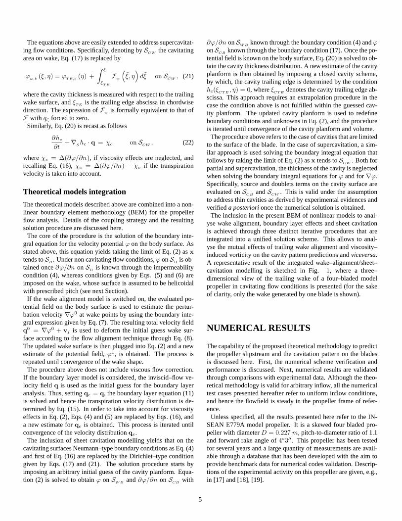
The inclusion in the present BEM of nonlinear models to anal-yse wake alignment, boundary layer effects and sheet cavitationis achieved through three distinct iterative procedures that areintegrated into a unified solution scheme. This allows to anal-yse the mutual effects of trailing wake alignment and viscosity–induced vorticity on the cavity pattern predictions andviceversa.A representative result of the integrated wake–alignment/sheet–cavitation modelling is sketched in Fig. 1, where a three–dimensional view of the trailing wake of a four–bladed modelpropeller in cavitating flow conditions is presented (for the sakeof clarity, only the wake generated by one blade is shown).

NUMERICAL RESULTS

The capability of the proposed theoretical methodology to predictthe propeller slipstream and the cavitation pattern on the bladesis discussed here. First, the numerical scheme verification andperformance is discussed. Next, numerical results are validatedthrough comparisons with experimental data. Although the theo-retical methodology is valid for arbitrary inflow, all the numericaltest cases presented hereafter refer to uniform inflow conditions,and hence the flowfield is steady in the propeller frame of refer-ence.

Unless specified, all the results presented here refer to the IN-SEAN E779A model propeller. It is a skewed four bladed pro-peller with diameterD = 0.227 m, pitch-to-diameter ratio of 1.1and forward rake angle of43′′. This propeller has been testedfor several years and a large quantity of measurements are avail-able through a database that has been developed with the aim toprovide benchmark data for numerical codes validation. Descrip-tions of the experimental activity on this propeller are given, e.g.,in [17] and [18], [19].

5

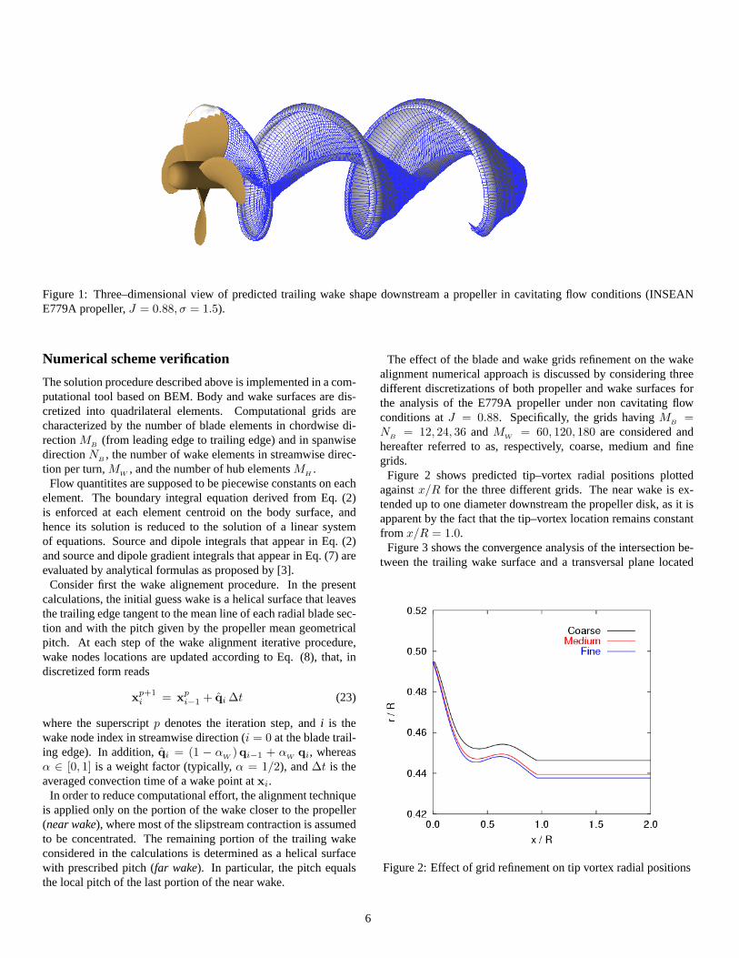
Figure 1: Three–dimensional view of predicted trailing wake shape downstream a propeller in cavitating flow conditions (INSEANE779A propeller,J = 0.88, σ = 1.5).

Numerical scheme verification

The solution procedure described above is implemented in a com-putational tool based on BEM. Body and wake surfaces are dis-cretized into quadrilateral elements. Computational grids arecharacterized by the number of blade elements in chordwise di-rectionM

B(from leading edge to trailing edge) and in spanwise

directionNB

, the number of wake elements in streamwise direc-tion per turn,M

W, and the number of hub elementsM

H.

Flow quantitites are supposed to be piecewise constants on eachelement. The boundary integral equation derived from Eq. (2)is enforced at each element centroid on the body surface, andhence its solution is reduced to the solution of a linear systemof equations. Source and dipole integrals that appear in Eq. (2)and source and dipole gradient integrals that appear in Eq. (7) areevaluated by analytical formulas as proposed by [3].

Consider first the wake alignement procedure. In the presentcalculations, the initial guess wake is a helical surface that leavesthe trailing edge tangent to the mean line of each radial blade sec-tion and with the pitch given by the propeller mean geometricalpitch. At each step of the wake alignment iterative procedure,wake nodes locations are updated according to Eq. (8), that, indiscretized form reads

xp+1i = xp

i−1 + qi ∆t (23)

where the superscriptp denotes the iteration step, andi is thewake node index in streamwise direction (i = 0 at the blade trail-ing edge). In addition,qi = (1 − α

W)qi−1 + α

Wqi, whereas

α ∈ [0, 1] is a weight factor (typically,α = 1/2), and∆t is theaveraged convection time of a wake point atxi.

In order to reduce computational effort, the alignment techniqueis applied only on the portion of the wake closer to the propeller(near wake), where most of the slipstream contraction is assumedto be concentrated. The remaining portion of the trailing wakeconsidered in the calculations is determined as a helical surfacewith prescribed pitch (far wake). In particular, the pitch equalsthe local pitch of the last portion of the near wake.

The effect of the blade and wake grids refinement on the wakealignment numerical approach is discussed by considering threedifferent discretizations of both propeller and wake surfaces forthe analysis of the E779A propeller under non cavitating flowconditions atJ = 0.88. Specifically, the grids havingM

B=

NB

= 12, 24, 36 and MW

= 60, 120, 180 are considered andhereafter referred to as, respectively, coarse, medium and finegrids.

Figure 2 shows predicted tip–vortex radial positions plottedagainstx/R for the three different grids. The near wake is ex-tended up to one diameter downstream the propeller disk, as it isapparent by the fact that the tip–vortex location remains constantfrom x/R = 1.0.

Figure 3 shows the convergence analysis of the intersection be-tween the trailing wake surface and a transversal plane located

Figure 2: Effect of grid refinement on tip vortex radial positions

6

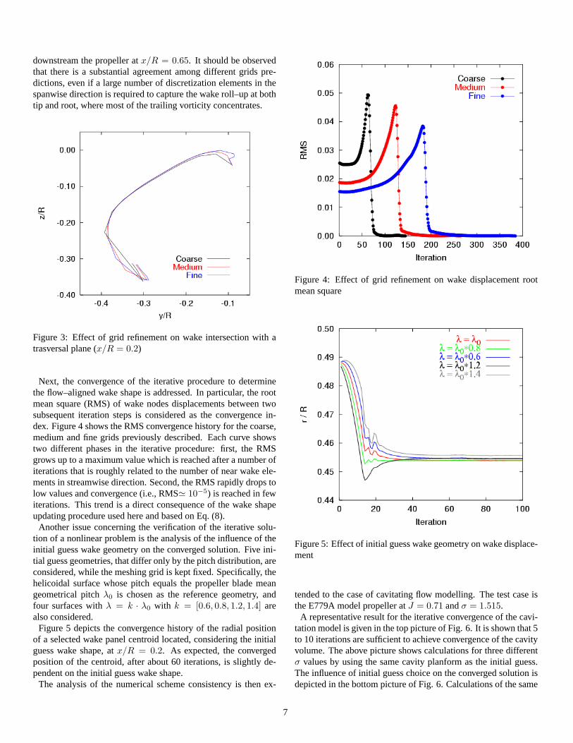
downstream the propeller atx/R = 0.65. It should be observedthat there is a substantial agreement among different grids pre-dictions, even if a large number of discretization elements in thespanwise direction is required to capture the wake roll–up at bothtip and root, where most of the trailing vorticity concentrates.

Figure 3: Effect of grid refinement on wake intersection with atrasversal plane (x/R = 0.2)

Next, the convergence of the iterative procedure to determinethe flow–aligned wake shape is addressed. In particular, the rootmean square (RMS) of wake nodes displacements between twosubsequent iteration steps is considered as the convergence in-dex. Figure 4 shows the RMS convergence history for the coarse,medium and fine grids previously described. Each curve showstwo different phases in the iterative procedure: first, the RMSgrows up to a maximum value which is reached after a number ofiterations that is roughly related to the number of near wake ele-ments in streamwise direction. Second, the RMS rapidly drops tolow values and convergence (i.e., RMS' 10−5) is reached in fewiterations. This trend is a direct consequence of the wake shapeupdating procedure used here and based on Eq. (8).

Another issue concerning the verification of the iterative solu-tion of a nonlinear problem is the analysis of the influence of theinitial guess wake geometry on the converged solution. Five ini-tial guess geometries, that differ only by the pitch distribution, areconsidered, while the meshing grid is kept fixed. Specifically, thehelicoidal surface whose pitch equals the propeller blade meangeometrical pitchλ0 is chosen as the reference geometry, andfour surfaces withλ = k · λ0 with k = [0.6, 0.8, 1.2, 1.4] arealso considered.

Figure 5 depicts the convergence history of the radial positionof a selected wake panel centroid located, considering the initialguess wake shape, atx/R = 0.2. As expected, the convergedposition of the centroid, after about 60 iterations, is slightly de-pendent on the initial guess wake shape.

The analysis of the numerical scheme consistency is then ex-

Figure 4: Effect of grid refinement on wake displacement rootmean square

Figure 5: Effect of initial guess wake geometry on wake displace-ment

tended to the case of cavitating flow modelling. The test case isthe E779A model propeller atJ = 0.71 andσ = 1.515.

A representative result for the iterative convergence of the cavi-tation model is given in the top picture of Fig. 6. It is shown that 5to 10 iterations are sufficient to achieve convergence of the cavityvolume. The above picture shows calculations for three differentσ values by using the same cavity planform as the initial guess.The influence of initial guess choice on the converged solution isdepicted in the bottom picture of Fig. 6. Calculations of the same

7

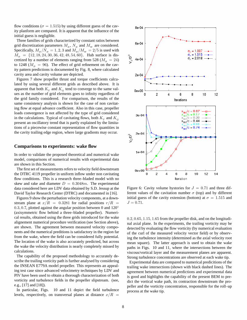
flow conditions (σ = 1.515) by using different guess of the cav-ity planform are compared. It is apparent that the influence of theinitial guess is negligible.

Three families of grids characterized by constant ratios betweengrid discretization parametersM

B, N

BandM

Ware considered.

Specifically,MB/N

B= 1, 2, 3 andM

B/M

W= 2/5 is used with

MB

= 12, 18, 24, 30, 36, 42, 48, 54, 60. Hub surface is dis-cretized by a number of elements ranging from 528 (M

B= 24)

to 1248 (MB

= 96). The effect of grid refinement on the cav-ity pattern predictions is documented by Fig. 8, where calculatedcavity area and cavity volume are depicted.

Figures 7 show propeller thrust and torque coefficients calcu-lated by using several different grids as described above. It isapparent that bothK

TandK

Qtend to converge to the same val-

ues as the number of grid elements goes to infinity regardless ofthe grid family considered. For comparison, the results of thesame consistency analysis is shown for the case of non cavitat-ing flow at equal advance coefficient. Also in this case, propellerloads convergence is not affected by the type of grid consideredin the calculations. Typical of cavitating flows, bothK

TandK

Q

present an oscillatory trend that is partly explained by the limita-tions of a piecewise constant representation of flow quantities inthe cavity trailing edge region, where large gradients may occur.

Comparisons to experiments: wake flow

In order to validate the proposed theoretical and numerical wakemodel, comparisons of numerical results with experimental dataare shown in this Section.

The first set of measurements refers to velocity field downstreamthe DTRC 4119 propeller in uniform inflow under non cavitatingflow conditions. This is a research three–bladed model with noskew and rake and diameterD = 0.3048m. The experimentaldata considered here are LDV data obtained by S.D. Jessup at theDavid Taylor Research Center (DTRC) and documented in [16].

Figures 9 show the perturbation velocity components, at a down-stream plane atx/R = 0.3281 for radial positionsr/R =0.3, 0.7, plotted against the angular position between 0 and 120

(axisymmetric flow behind a three–bladed propeller). Numeri-cal results, obtained using the three grids introduced for the wakealignement numerical procedure verification (see Section above),are shown. The agreement between measured velocity compo-nents and the numerical preditions is satisfactory in the region farfrom the wake, where the field can be considered fully potential.The location of the wake is also accurately predicted, but acrossthe wake the velocity distribution is nearly completely missed bycalculations.

The capability of the proposed methodology to accurately de-scribe the trailing vorticity path is further analysed by consideringthe INSEAN E779A model propeller. This represents an appeal-ing test case since advanced velocimetry techniques by LDV andPIV have been used to obtain a thorough characterization of bothvorticity and turbulence fields in the propeller slipstream. (see,e.g., [17] and [18]).

In particular, Figs. 10 and 11 depict the field turbulencelevels, respectively, on transversal planes at distancex/R =

Figure 6: Cavity volume hystories forJ = 0.71 and three dif-ferent values of the cavitation numberσ (top) and by differentinitial guess of the cavity extension (bottom) atσ = 1.515 andJ = 0.71.

0.2, 0.65, 1.15, 1.65 from the propeller disk, and on the longitudi-nal axial plane. In the experiments, the trailing vorticity may bedetected by evaluating the flow vorticity (by numerical evaluationof the curl of the measured velocity vector field) or by observ-ing the turbulence intensity (determined as the axial velocity rootmean square). The latter approach is used to obtain the wakepaths in Figs. 10 and 11, where the intersections between theviscous/vortical layer and the measurement planes are apparent.Strong turbulence concentrations are observed at each wake tip.

Experimental data are compared to numerical predicitions of thetrailing wake intersections (shown with black dashed lines). Theagreement between numerical predictions and experimental datais good and highlights the capability of the present BEM to pre-dict the vortical wake path, its contraction downstream the pro-peller and the vorticity concentration, responsible for the roll–upprocess at the wake tip.

8

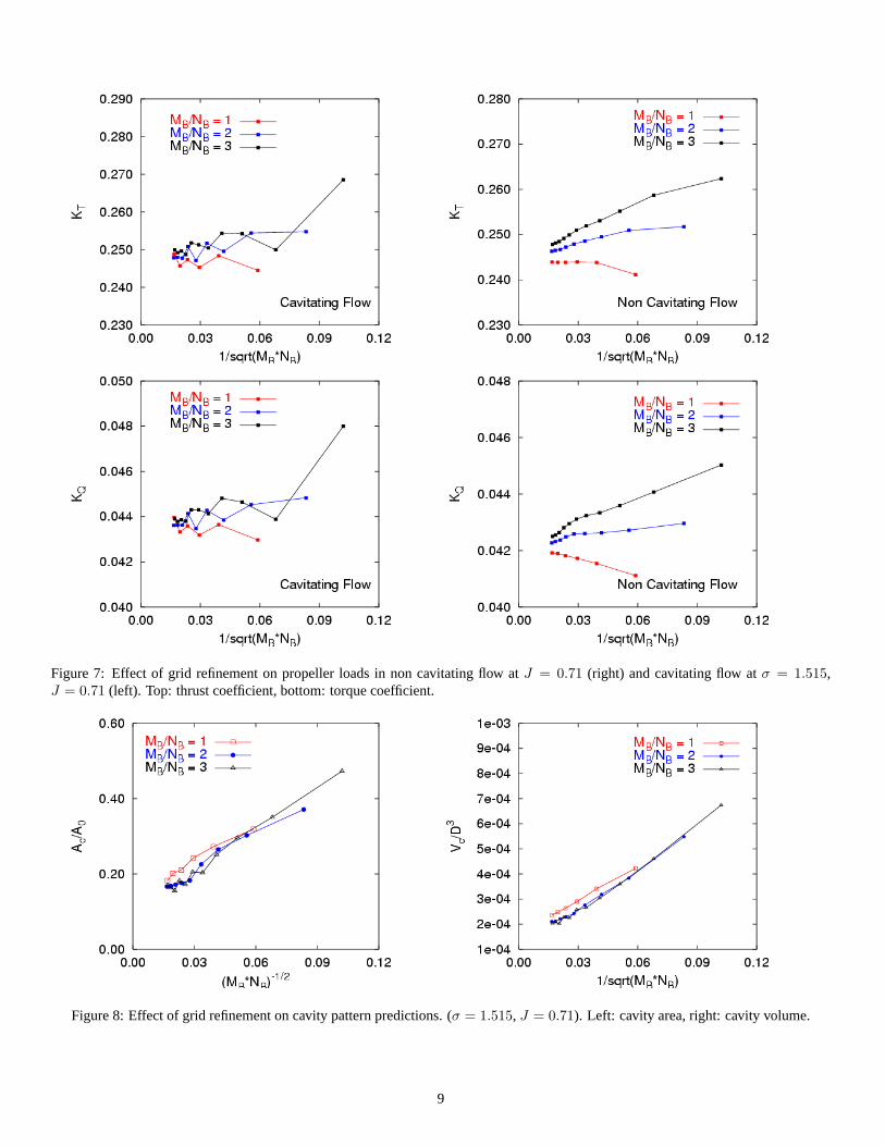
Figure 7: Effect of grid refinement on propeller loads in non cavitating flow atJ = 0.71 (right) and cavitating flow atσ = 1.515,J = 0.71 (left). Top: thrust coefficient, bottom: torque coefficient.

Figure 8: Effect of grid refinement on cavity pattern predictions. (σ = 1.515, J = 0.71). Left: cavity area, right: cavity volume.

9

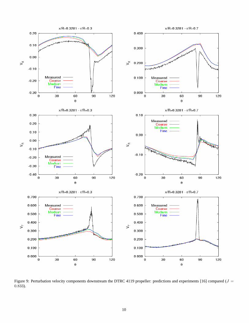
Figure 9: Perturbation velocity components downstream the DTRC 4119 propeller: predictions and experiments [16] compared (J =0.833).

10

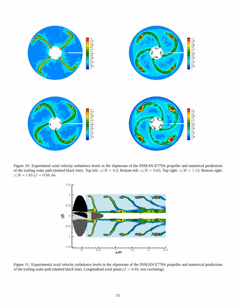
Figure 10: Experimentl axial velocity turbulence levels in the slipstream of the INSEAN E779A propeller and numerical predictionsof the trailing wake path (dashed black line). Top left:x/R = 0.2; Bottom left: x/R = 0.65; Top right: x/R = 1.15; Bottom right:x/R = 1.65 (J = 0.88, non cavitating).

Figure 11: Experimental axial velocity turbulence levels in the slipstream of the INSEAN E779A propeller and numerical predictionsof the trailing wake path (dashed black line). Longitudinal axial plane (J = 0.88, non cavitating).

11

Comparisons to experiments: cavitation pattern

The capability of the integrated BEM methodology to accuratelydescribe the evolution of sheet cavities on the propeller bladesis addressed here. Numerical results are validated through com-parisons with experimental data for the INSEAN E779A modelpropeller.

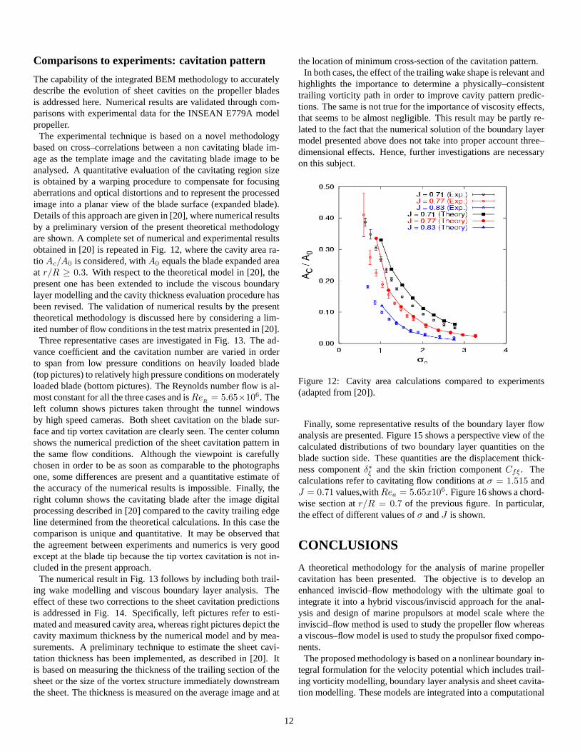
The experimental technique is based on a novel methodologybased on cross–correlations between a non cavitating blade im-age as the template image and the cavitating blade image to beanalysed. A quantitative evaluation of the cavitating region sizeis obtained by a warping procedure to compensate for focusingaberrations and optical distortions and to represent the processedimage into a planar view of the blade surface (expanded blade).Details of this approach are given in [20], where numerical resultsby a preliminary version of the present theoretical methodologyare shown. A complete set of numerical and experimental resultsobtained in [20] is repeated in Fig. 12, where the cavity area ra-tio Ac/A0 is considered, withA0 equals the blade expanded areaat r/R ≥ 0.3. With respect to the theoretical model in [20], thepresent one has been extended to include the viscous boundarylayer modelling and the cavity thickness evaluation procedure hasbeen revised. The validation of numerical results by the presenttheoretical methodology is discussed here by considering a lim-ited number of flow conditions in the test matrix presented in [20].

Three representative cases are investigated in Fig. 13. The ad-vance coefficient and the cavitation number are varied in orderto span from low pressure conditions on heavily loaded blade(top pictures) to relatively high pressure conditions on moderatelyloaded blade (bottom pictures). The Reynolds number flow is al-most constant for all the three cases and isRe

R= 5.65×106. The

left column shows pictures taken throught the tunnel windowsby high speed cameras. Both sheet cavitation on the blade sur-face and tip vortex cavitation are clearly seen. The center columnshows the numerical prediction of the sheet cavitation pattern inthe same flow conditions. Although the viewpoint is carefullychosen in order to be as soon as comparable to the photographsone, some differences are present and a quantitative estimate ofthe accuracy of the numerical results is impossible. Finally, theright column shows the cavitating blade after the image digitalprocessing described in [20] compared to the cavity trailing edgeline determined from the theoretical calculations. In this case thecomparison is unique and quantitative. It may be observed thatthe agreement between experiments and numerics is very goodexcept at the blade tip because the tip vortex cavitation is not in-cluded in the present approach.

The numerical result in Fig. 13 follows by including both trail-ing wake modelling and viscous boundary layer analysis. Theeffect of these two corrections to the sheet cavitation predictionsis addressed in Fig. 14. Specifically, left pictures refer to esti-mated and measured cavity area, whereas right pictures depict thecavity maximum thickness by the numerical model and by mea-surements. A preliminary technique to estimate the sheet cavi-tation thickness has been implemented, as described in [20]. Itis based on measuring the thickness of the trailing section of thesheet or the size of the vortex structure immediately downstreamthe sheet. The thickness is measured on the average image and at

the location of minimum cross-section of the cavitation pattern.In both cases, the effect of the trailing wake shape is relevant and

highlights the importance to determine a physically–consistenttrailing vorticity path in order to improve cavity pattern predic-tions. The same is not true for the importance of viscosity effects,that seems to be almost negligible. This result may be partly re-lated to the fact that the numerical solution of the boundary layermodel presented above does not take into proper account three–dimensional effects. Hence, further investigations are necessaryon this subject.

Figure 12: Cavity area calculations compared to experiments(adapted from [20]).

Finally, some representative results of the boundary layer flowanalysis are presented. Figure 15 shows a perspective view of thecalculated distributions of two boundary layer quantities on theblade suction side. These quantities are the displacement thick-ness componentδ∗ξ and the skin friction componentCfξ. Thecalculations refer to cavitating flow conditions atσ = 1.515 andJ = 0.71 values,withRea = 5.65x106. Figure 16 shows a chord-wise section atr/R = 0.7 of the previous figure. In particular,the effect of different values ofσ andJ is shown.

CONCLUSIONS

A theoretical methodology for the analysis of marine propellercavitation has been presented. The objective is to develop anenhanced inviscid–flow methodology with the ultimate goal tointegrate it into a hybrid viscous/inviscid approach for the anal-ysis and design of marine propulsors at model scale where theinviscid–flow method is used to study the propeller flow whereasa viscous–flow model is used to study the propulsor fixed compo-nents.

The proposed methodology is based on a nonlinear boundary in-tegral formulation for the velocity potential which includes trail-ing vorticity modelling, boundary layer analysis and sheet cavita-tion modelling. These models are integrated into a computational

12

tool based on BEM.Numerical results have been presented to analyse the numerical

scheme in terms of iterative convergence and sensitivity of resultswith respect to the computational grids. Next, numerical pre-dictions validation has been discussed through comparisons withexperimental data. The capability to evaluate the velocity fieldand the vorticity path in the propeller slipstream has been demon-strated. This is a necessary step to obtain accurate predictions ofthe propeller loads and to develop numerical models of the tip–vortex cavitation. Sheet cavitation predictions have been assessedthrough comparisons with high–quality experimental data. Theeffects of both trailing vorticity and of the boundary layer flowon cavitation have been investigated. In particular, it is observedthat the shape of the wake has a relevant impact on the cavitypattern prediction, even in the case of partial cavities that do notextend to the wake. On the contrary, a direct effect of the viscos-ity correction on the cavity pattern is almost negligible. However,it should be recalled that the boundary layer solution interactswith the wake alignment technique through the evaluation of thesize of the vortex core, and hence the viscosity correction impactsindirectly with the cavitation analysis through the trailing wakevorticity.

Improvements of the numerical solution of the boundary layerequations is the primary aim of further developments of thepresent theroretical model.

References

[1] Kim, Y. G. and Lee, C. S. (1997). ‘Prediction of UnsteadyPerformance of Marine Propellers with Cavitation UsingSurface-Panel Method.’Proceedings of the Twenty-firstSymposium on Naval Hydrodynamics, Trondheim (Nor-way), pp. 913-929.

[2] Kinnas, S.A., Fine, N.E. (1992). ‘A Nonlinear Boundary El-ement Method for the Analysis of Unsteady Propeller SheetCavitation,’Proceedings of the nineteenth ONR Symposiumon Naval Hydrodynamics, Seoul (Korea) 1992, pp. 717–737.

[3] Morino, L, Chen, L.T., Suciu, E. (1975). ‘Steady and Os-cillatory Subsonic and Supersonic Aerodynamics AroundComplex Configurations,’AIAA Journal, Vol. 13, 1975, pp.368–374.

[4] Suciu E.O., Morino, L., A nonlinear finite element analy-sis of wing in steady incompressible flows with wake roll-up, AIAA 14th Aerospace Sciences Meeting, WashingtonD.C., 1976.

[5] Campbell, R.G.,Foundations of fluid flow theory, Addison-Wesley, Reading, Massachusetts, 1973.

[6] Salvatore, F., Testa, C. (2002). ‘Theoretical Modelling ofMarine Propeller Cavitation in Unsteady High-ReynoldsNumber Flows.’ INSEAN Report 2002-077, Rome (Italy).

[7] Cousteix, J. (1986), ‘Three Dimensional Boundary Lay-ers. Introduction to Calculation Methods.’ Advisory Report741, AGARD.

[8] Nishida, B.A., (1996). ‘Fully Simultaneous Coupling of theFull Potential Equations and the Integrated Boundary LayerEquations in Three Dimensions.’ Doctoral thesis, M.I.T.,Massachussetts (USA).

[9] Thwaites, B. (1949). Approximate calculation of the laminarboundary layer.Aeronaut. Quart.,1, pp. 245–280, 1949.

[10] Michel, R. (1952). Etude de la transition sur les profils d’aile- establissment d’un point de transition et calcul de la traineede profil en incompressible.ONERA Tech. Rep.1/1578A.

[11] Green, J.E., Weeks, D.J., Brooman, W.F. (1973). Predic-tion of turbulent boundary layers and wakes in compress-ible flow by a lag–entrainment method.A.R.C.R. & M.Tech. Rep.3791.

[12] Johnston, J.P., (1957). ‘Three Dimensional turbulent Bound-ary Layers.’ Doctoral thesis, M.I.T., Massachussetts (USA).

[13] Lighthill, M.J. (1958). On displacement thickness.J. FluidMech.,4, pp. 383–392.

[14] Morino, L., Salvatore, F., Gennaretti, M. (1997). ‘A NewVelocity Decomposition for Viscous Flows: Lighthill’sEquivalent–Source Method Revisited’.Computer Methodsin Applied Mechanics and Engineering, Vol. 173, No. 3–4,pp. 317–336, 1999.

[15] Lemonnier, H. & Rowe, A. (1988), ‘Another Approach inModelling Cavitating Flows,’Journal of Fluid Mechanics,Vol. 195, pp. 557–580.

[16] Jessup, S.D. (1989). Jessup, S.D., An experimental investi-gation of viscous aspects of propeller blade flows,PhD the-sis, The Catholic Univ. of America, 1989.

[17] Di Felice, F. and Romano, G. P. and Elefante, M. (2000).‘Propeller Wake Evolution by Means of PIV.’Proceedingsof the 23 rd ONR Symposium on Naval Hydrodynamics,Val de Reuil (France).

[18] Stella, A. and Guj, G. and Di Felice, F. (2000). ‘PropellerFlow Field Analysis by Means of LDV Phase SamplingTechniques.’Experiments in Fluids, Vol. 28, pp. 1–10.

[19] Di Florio, D., Di Felice, F., Felli, F., Romano, G.P. (2003).‘Experimental Investigation of the Propeller Wake at Differ-ent Loading Condition by PIV,’ accepted for publication onJournal of ship Research.

[20] Pereira, F., Salvatore, F., Di Felice, F., Elefante, M. (2002).‘Experimental and Numerical Investigation of the Cavita-tion Pattern on a Marine Propeller’,Proceedings of the24 rd ONR Symposium on Naval Hydrodynamics, Fukuoka(Japan).

13

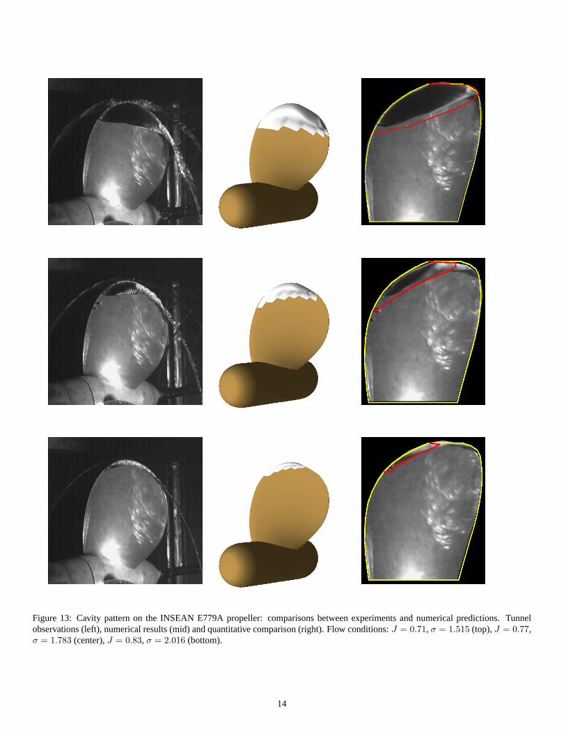
Figure 13: Cavity pattern on the INSEAN E779A propeller: comparisons between experiments and numerical predictions. Tunnelobservations (left), numerical results (mid) and quantitative comparison (right). Flow conditions:J = 0.71, σ = 1.515 (top),J = 0.77,σ = 1.783 (center),J = 0.83, σ = 2.016 (bottom).

14

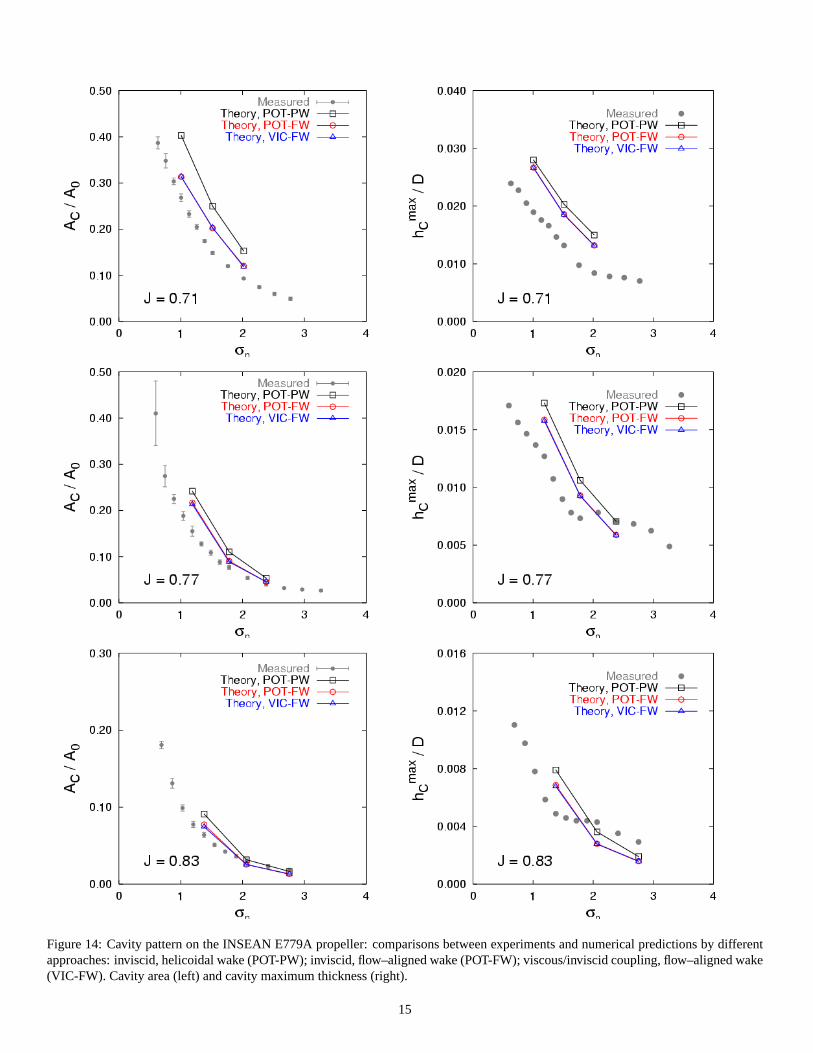
Figure 14: Cavity pattern on the INSEAN E779A propeller: comparisons between experiments and numerical predictions by differentapproaches: inviscid, helicoidal wake (POT-PW); inviscid, flow–aligned wake (POT-FW); viscous/inviscid coupling, flow–aligned wake(VIC-FW). Cavity area (left) and cavity maximum thickness (right).

15

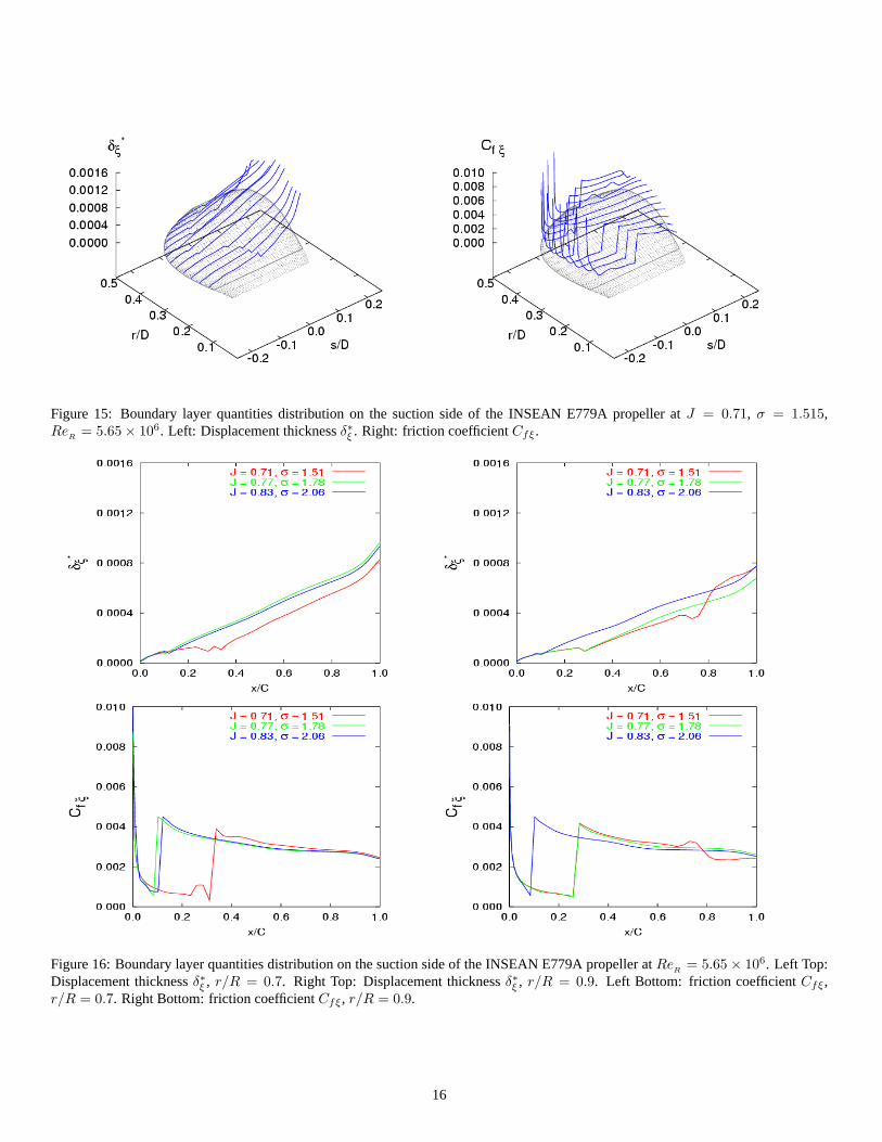
Figure 15: Boundary layer quantities distribution on the suction side of the INSEAN E779A propeller atJ = 0.71, σ = 1.515,Re

R= 5.65× 106. Left: Displacement thicknessδ∗ξ . Right: friction coefficientCfξ.

Figure 16: Boundary layer quantities distribution on the suction side of the INSEAN E779A propeller atReR

= 5.65× 106. Left Top:Displacement thicknessδ∗ξ , r/R = 0.7. Right Top: Displacement thicknessδ∗ξ , r/R = 0.9. Left Bottom: friction coefficientCfξ,r/R = 0.7. Right Bottom: friction coefficientCfξ, r/R = 0.9.

16