Complex-grid spectral algorithms for inviscid linear instability of boundary-layer flows

V. Theofilis a'*, A. Karabis b, S.J. Shaw c

a DLR, Institute of Fluid Mechantes, Bunsenstrafie 10, D-37073 Gbttingen, Germany b Department of Mathematics, University of Pairas, GR-26500 Pairas, Greece

c Applied Mathematics and Operational Research Group, Cranfield University, RMCS Shrivenham, Swindon SN6 8LA, UK

Abstract

We present a suite of algorithms designed to obtain aecurate numerical solutions of the generalised ei-genvalue problem governing inviscid linear instability of boundary-layer type of flow in both the incom­pressible and compressible regimes on planar and axisymmetric curved geometries. The large gradient problems which oceur in the governing equations at critical layers are treated by diverting the integration path into the complex plañe, making use of complex mappings. The need for expansión of the basic flow profiles in truncated Taylor series is circumvented by solving the boundary-layer equations directly on the same (complex) grid used for the instability calculations. Iterative and direct solution algorithms are em-ployed and the performance of the resulting algorithms using nonlinear radiation or homogeneous Di-richlet far-field boundary conditions is examined. The dependence of the solution on the parameters of the complex mappings is discussed. Results of incompressible and supersonic flow examples are presented; their excellent agreement with established works demonstrates the aecuracy and robustness of the new methods presented. Means of improving the efficieney of the proposed spectral algorithms are suggested. © 2002 Elsevier Science Ltd. All rights reserved.

1. Introduction

Interest in boundary-layer linear flow instability developed in the late parts of the 19th and the early parts of last century in the quest for the description of deterministic routes of laminar-turbulent flow transition. Linear theory is still erroneously taken to be exclusively applicable to

* Corresponding author. Tel.: +49-551-709-2430; fax: +49-551-709-2404. E-mail address: vassilios.theofilis@dlr.de (V. Theofilis).

flows in which two out of three spatial directions are taken to be homogeneous and treated as periodic, as required by the early analyses (the reader is referred to Drazin and Reid [5] for an overview), or to flows in which weak basic (boundary-layer type) flow variation is admitted in one spatial direction, the second spatial direction is taken to be periodic and the third is resolved [14]. Today we are in a position to redefine the boundaries of a linear analysis by considering the instability of flow to small-amplitude disturbances which are periodic in one spatial direction alone, the other two spatial directions being resolved numerically (e.g. [32], and references therein). Discussion of the latter global linear theory is beyond the scope of the present paper; here we confine ourselves to the bounds of the classic linear analysis which is concerned with wave-like disturbances whose amplitudes are functions of one spatial direction alone. Such disturbances have been observed experimentally, although comparisons with the theory have been met with mixed success. Most notable verification of the classic linear theory has been the experiments of Schubauer and Skramstad [27] where Tollmien-Schlichting (TS) instabilities were observed in incompressible flat-plate boundary-layer flow at a time when only the Góttingen school of Prandtl had faith in the theory; probably the most notable failure of the theory is its prediction of stability of pipe Poiseuille flow at all Reynolds numbers, although instability is known to exist in this flow at low Reynolds numbers at least since Reynolds [26] conducted his famous experiments in Manchester.

Strong ímpetus was offered to the theory of linear flow instability by the development of nu-merical techniques, based on finite-differences, for the solution of both the inviscid and the viscous linear eigenvalue problem. The pioneering eflbrts of Mack [18,19] were crowned with the dis-covery of a sequence of new modes particular to compressible flow which have been verified experimentally to exist in both planar and axisymmetric geometries [21]. Here the term 'mode' is used to describe members of either the discrete or continuous finite spectrum of eigenvalues re-sulting from numerical solution of the generalised eigenvalue problem which forms the basis of a temporal or spatial linear instability analysis. The first mode of instability is the compressible analogue of the discrete TS mode of incompressible flow, while the second and higher so-called Mack modes are unique to supersonic (and hypersonic) flows. Mack's work on the problem of the linear instability of boundary-layer flow in planar geometries was complemented by the seminal work of Duck [6] who dealt with the inviscid instability problem of boundary-layer flow in axi­symmetric geometries. Duck and Shaw [8] (DS) and Shaw and Duck [28] considered the eflects that wall curvature has on the planar compressible observations of Mack, concentrating on the first two unstable modes.

What makes inviscid linear instability theory interesting from a physical point of view is that in compressible flow the existence of inflectional profiles of the basic flow results in the instability mechanism to be inviscid in nature with viscosity acting to diminish the growth rates of insta­bilities. On the other hand, what makes the inviscid instability problem interesting from a numerical point of view is the possible existence of what are termed critical points which cor-respond to singularities of the governing equations. In temporal linear instability theory these are locations where the disturbance phase speed equals that of the streamwise basic flow velocity, while in spatial theory it is where the ratio of frequency to wavenumber equals the streamwise basic flow velocity. Singularities only occur when the eigenvalue being sought is real, Le., neutral disturbances. However, for complex eigenvalues (both growing and decaying disturbances) the imaginary part is typically small and thus results in sharp gradients in a región termed the critical

layer. The existence of critical layers in an inviscid framework prohibits the use of straightfor-ward spectral collocation techniques (e.g. [17]) for the numerical solution of the inviscid incompressible or compressible linear instability problem. The numerical algorithms of Duck [6] are typical of methods currently used in linear instability analysis. The steady basic flow is obtained by employing the boundary-layer approximation, in which the resultant system of equations is solved using a Crank-Nicolson finite-difference scheme with suitable boundary conditions. The instability equations are solved using a fourth-order accurate Runge-Kutta shooting scheme, beginning the shooting process at a suitably chosen valué in the far field where radiation (as opposed to homogeneous Dirichlet) boundary conditions are imposed and the computation proceeds inwards to the fixed boundary. The eigenvalues are determined so that the impermeability condition on the surface of the axisymmetric bodies is satisfied. This is achieved by making an initial guess and then, through the use of a Newton-iteration scheme, the shooting process is repeated until preset convergence criteria are met. To deal with critical layer problems the contour indentation method of Zaat [33] and Mack [18] is employed, with basic flow quantities being approximated by truncated power series in the complex plañe.

While (real-grid) spectral methods have long been applied to the solution of the basic flow problem [25] their application to the resultant inviscid instability analysis has proved prohibitive due to the existence of the critical layers, as remarked upon above. Note, in many cases the eigenvalue lies sufficiently far from the real axis such that convergence rates are only slightly affected. In such cases a standard (real-grid) spectral discretisation is adequate. However, for most of the boundary layers of the type considered in this paper the imaginary parts of the eigenvalues are of the order of 10~3 or less, as can be seen in Section 4. The simple-minded approach of grid refinement, aside from being computationally intensive on account of the dense spectral collocation matrices, does not alleviate the problem for neutral disturbances or where the eigenvalue imaginary part is very small. Two solutions are known to us in order to regain spectral accuracy. The first is to use a standard Chebyshev Gauss-Lobatto (real) grid [4] but Taylor-expand the basic flow around the critical layer. The second, followed herein, is to extend the Zaat-Mack technique for the integration of the instability equations in the complex plañe and introduce complex collocation grids, forcing a spectral method to intégrate the equations on a complex contour suitably adapted to avoid the critical layer. Use of this second approach was first suggested by Boyd and Christidis [2] and further investigated by Boyd [1] in the context of atmospheric and hydrodynamic instability calculations. These works were extended by Gilí and Sneddon [11], who gave an analytic formula for optimizing one family of complex (quadratic) maps. Gilí and Sneddon [12] also developed a new technique based on composite complex maps to handle near-boundary critical points. Their work involved calculating the eigenvalues of linearized hydrodynamic instability and Sturm-Liouville eigenproblems of the fourth kind. Mayer and Powell [23] investigated the instability of a trailing vortex, while in the recent work of Fang and Reshotko [9,10] the inviscid spatial stability of a developing axisymmetric mixing layer was investigated. Mayer and Powell [23] state that in the instability problem they consid­ered:

"Without any deformation, the eigenvalue corresponding to the primary mode is inaccessi-ble no matter how many basis functions are used."

They showed that the combination of a complex grid and the spectral method is essential for the inviscid linear analysis of their trailing vortex model problem. Duck et al. [7] also found that the same approach for the instability equations of compressible plañe Couette flow delivers accurate results (prívate communication, 2000) although no discussion of this issue using a spectral method was presented in [7].

Here we revisit typical inviscid linear instability problems encountered in wall-bounded boundary-layer type of external aerodynamic flows and discuss a novel spectral scheme for the solution of the incompressible inviscid linear eigenvalue problem in planar geometries and that pertaining to supersonic flow in both planar and axisymmetric curved geometries. The first problem is governed by the classic Rayleigh equation while compressibility and curvature are discussed using the equations of Duck [6] or their planar limits. We employ complex spectral collocation grid techniques first to the solution of the basic flow problem and subsequently to both the incompressible and the compressible inviscid linear eigenvalue problems. The accuracy and the efficiency of the proposed algorithms are assessed in comprehensive comparisons of re­sults obtained using our spectral approach against the work of Mack [19,20] and the finite-dif-ference algorithm of Duck [6]. In either the incompressible or the compressible case several concerns arise. First, the effect of closing either the incompressible or the compressible system of governing equations by the straightforward homogeneous Dirichlet boundary conditions or by the appropriate radiation far-field boundary conditions is unknown and must be examined. This issue has been successfully resolved by Macaraeg et al. [17] in the context of viscous real-grid spectral collocation calculations; here we extend the discussion to inviscid calculations based on complex spectral collocation grids for the case of compressible boundary layers. Second, the performance of complex-grid techniques in combination with the two most widely used strategies for the calculation of the eigenspectrum, namely global and local methods, must be examined; results have been obtained using the QZ algorithm as well as a Newton-iteration scheme. Algo­rithms for the solution of the individual numerical problems cited are combined to form a spectrally accurate method for the solution of inviscid linear instability problems in boundary-layer type of flows. In Section 2 we present the theoretical framework for the compressible inviscid linear instability problem in axisymmetric geometries from which the compressible and incom­pressible planar problems are derived. In Section 3 the building blocks of our numerical ap-proaches are detailed. Results are presented first for the basic flow and subsequently for the incompressible and compressible eigenvalue problems in Section 4. Conclusions are furnished in Section 5. We use Appendices A and B to present technical details.

2. Inviscid linear instability theory of boundary-layer flow in axisymmetric geometries

We start by introducing the axisymmetric geometry, from which the planar limit is derived. The general layout of the problem is shown in Fig. 1. The z*-axis lies along the body axis, r* is the radial coordínate and 6 the azimuthal coordínate (superscript * denotes dimensional quantities). The curved body surface is taken to lie along r* = a* + X\z*, z* > 0, where a* is the tip radius, nonzero in the case of a cone and X\ denotes the slope parameter. The velocity vector has com-ponents v\, v*2 and v*3 in the r*, 9 and z* directions respectively. Also, U^ is the free-stream velocity in the axial direction, and p*^, ff^ and T^ represent the free-stream density, the first coefficient of

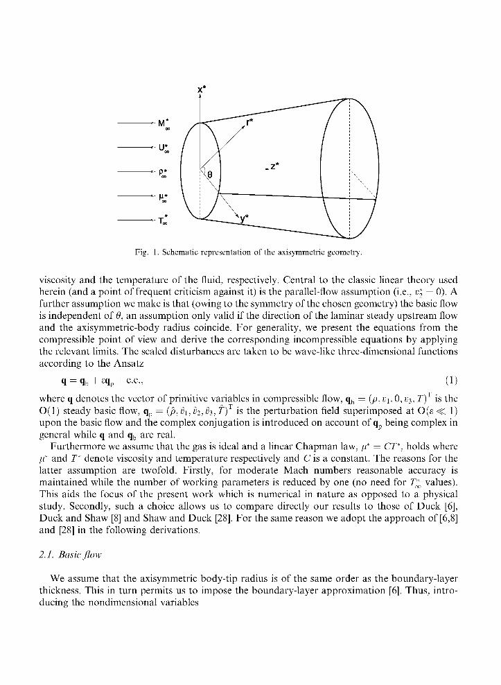
Fig. 1. Schematic representation of the axisymmetric geometry.

viscosity and the temperature of the fluid, respectively. Central to the classic linear theory used herein (and a point of frequent criticism against it) is the parallel-flow assumption (Le., v*2 = 0). A further assumption we make is that (owing to the symmetry of the chosen geometry) the basic flow is independent of 9, an assumption only valid if the direction of the laminar steady upstream flow and the axisymmetric-body radius coincide. For generality, we present the equations from the compressible point of view and derive the corresponding incompressible equations by applying the relevant limits. The scaled disturbances are taken to be wave-like three-dimensional functions according to the Ansatz

qb + eq + c . c , :i:

where q denotes the vector of primitive variables in compressible flow, qb = (p, v\, 0, u3, T) is the O(l) steady basic flow, qp = (p, i>\, v2, h, T) is the perturbation field superimposed at 0(e <C 1) upon the basic flow and the complex conjugation is introduced on account of qp being complex in general while q and qb are real.

Furthermore we assume that the gas is ideal and a linear Chapman law, p* = CT*, holds where p* and T* denote viscosity and temperature respectively and C is a constant. The reasons for the latter assumption are twofold. Firstly, for modérate Mach numbers reasonable accuracy is maintained while the number of working parameters is reduced by one (no need for T^ valúes). This aids the focus of the present work which is numerical in nature as opposed to a physical study. Secondly, such a choice allows us to compare directly our results to those of Duck [6], Duck and Shaw [8] and Shaw and Duck [28]. For the same reason we adopt the approach of [6,8] and [28] in the following derivations.

2.1. Basic flow

We assume that the axisymmetric body-tip radius is of the same order as the boundary-layer thickness. This in turn permits us to impose the boundary-layer approximation [6]. Thus, intro-ducing the nondimensional variables

xT ( P* Revi n v* T*\T

qb = (p,vh0,V3,T) = — , 7 ^ 7 7 , 0 , — , — , (2)

and, in addition

( '•"'-(¿•¡SF)1- (3)

where slender body divergence is assumed, i.e., X\ = CRe^1! where 1 ~ O(l), and implementing the transformation [8]

Vl=r%(ri,0, v3 = v3(r,,0, T = T(ri,0, (4)

where 2

the boundary-layer equations read [8]

_ 8Ü3 £hdh_- í tf+H\ ^1 = L— (rT—\ (7) Qr¡ 2 9£ V 2 / 8/7 r 8/7 l 8/7 i '

! - • <»>

where r = 1 +1£2 + C ,̂ and y is the ratio of specific heats, Mx the free-stream Mach number and a the Prandtl number. The boundary conditions, in the case of insulated walls with no mass transfer, are

6T vx =v3 = 0, — = 0 at n = 0, (10)

8?7

Ü3 - • 1, f ^ 1 as ?Í - • oo. (11)

2.2. Linear instability analysis

In order to determine the instability of the basic flow predicted by Eqs. (6)-(8)jve now perturb this flow by small-amplitude nonaxisymmetric disturbances qp = (p,üi,ü2,ü3, T) which have wavelengths of the same order as the boundary-layer thickness. The chosen frequency range of

disturbances also means that the parallel-flow approximation is asymptotically correct. At a given streamwise location z0 we represent the flow parameters by

P*=P*00[\/Mr)+sp{r)E]+0{s2),

v\ = EW*Jx{r)E + 0{E2),

v; = £U^v2(r)E + 0(82),

v; = U*JW0(r)+£v3(r)E]+O(82),

r = T*O0[T,{r) + 8T{r)E)+0{82),

p*=plR*T^[\+8p(r)E}+0(82),

where

£ = expi<9, W0{r)=v3{r,z0), T0{r) =T{r,z0),

t={U*Ja*)f, z = z*/a*.

(12)

(13)

(14)

(15)

(16)

(17)

(18)

(19)

Here qp = q E, e is a small parameter, 0 = a.z — cot + n6 with co the frequency and a the nondi-mensional wavenumber in spatial theory, while 0 = a.{z — ct) + n6 with a and c respectively de-noting wavenumber and wavespeed in temporal theory; in both cases n is the wavenumber in the azimuthal direction 6 (thus, a¡ < 0 implies spatial instability while c¡ > 0 implies temporal in­stability). Note, R* denotes the universal gas constant. Substituting the above into the full Navier-Stokes, energy and continuity equations and taking the 0(e)-terms with the leading order in Reynolds number (Le., ignoring viscous terms), a sixth-order system is obtained which can be reduced to the system [8]

% + í

•<P W0n<p 1/7

\+K2 + ín w,-fi yMi(W0-P)

2r2

1+- nK a 2 ( l+ lC 2 + Cí7)

•MKWO-P)1

•w2(Wü-p) Pn yMV

(20)

(21)

where cp = v\/t„ a. = a.t,, co = a>[, and P = c (c complex and a real) for temporal instability cal­culations while /? = co/a (a complex and co real) for spatial instability calculations. The boundary conditions are [8]

co =pn = 0 on r¡ = 0,

<P~^f{Kn+M+K^{n)} as oo,

(22)

(23)

p (PooM

2Jay(\ - P)KM

l-Mi(l-pf 1/2 as r¡ oo, (24)

where fj = ±a[ l — M¿(1 — /?)2]1/2(1/C + 1C + >7)J the sign of which is chosen such that the real part of the argument is positive in order for boundedness as r¡ —> oo to be ensured, cp^ is a constant and Kn{z\) denotes the modified Bessel function of order n and argument z\.

Alternatively, one may combine the system (20) and (21), into a single equation

2,^2 [Wo-PYM-

2„2 Cn

W« Of)

1 + -a 2 ( l + l C 2 + C ^

}p

\ + K2 + tv) *2(w0 - p)

subject to the boundary conditions

pn =0 for r¡ = 0,

P ~ T<PooM2J«.y{\ - P)Kn{n) / íl - Ml{\ - P)

:m-P) ToPn

ár] a2(W0-p)

1/2 as r¡ oo.

(25)

(26)

(27)

2.3. Planar limiting cases

To achieve the planar limits, we firstly set 1 = 0 in (20) and (21), Le., consider the cylinder form. Subsequently, the limit t, —> 0 is applied, corresponding to flow in planar geometries. This yields

W0tl(p _ <Pn _ 1P

W*-P yM2jW0-p) T0-M

¿JW0-PY

w2(Wü-p) Pn yM2J

(28)

(29)

which describe the inviscid linear instability of compressible boundary-layer flow in planar ge­ometries. Note, on applying the limit t, —> 0, one collapses onto plañe polar coordinates and not plañe cartesian coordinates. The corresponding boundary conditions are

(p=p =0 atf/ = 0,

and

<P ~ <Poo exp a.\ 1 ^-PfMln

ia.cPooyM^{\ - /?)exp

P

ccJi-ii-pYMin

I-(I-PYMÍ as r¡ —> oo.

(30)

(31)

(32)

Combining Eqs. (28) and (29) results in

[Wo-p)<pn-Wto,<p d_ dr¡

a? TM-P)<P. (33) ¿0 T0-Mi(W0-p)2

In the incompressible limit Mx —> 0 and T0 —> constant, so that

T^;[(W°-P)<P>I-W°>I<P]=T(W°-P)<P>

lo ar¡ i0

which may be rearranged to obtain the classic Rayleigh equation

{Wo-p) [<pm - a2 y] - W0mcp = 0, (34)

governing inviscid linear instability of incompressible boundary-layer flow in planar geometries.

3. Numerical methods

In this section we outline the numerical algorithms employed in this paper. We begin by pre-senting the complex mappings used in the wall-normal direction for both the basic flow and the instability calculations. Then the marching scheme for the basic flow is presented. We follow this with a discussion of the problems inherent in an inviscid linear instability analysis and present both global and iterative algorithms for their successful solution. The section concludes with a presentation of the boundary conditions used to cióse the alternative forms of the linear inviscid instability eigenvalue problem. All the calculations presented in this work were performed using 64-bit arithmetic.

3.1. Complex grids and corresponding mappings used

In all numerical work that follows we employ Chebyshev spectral collocation schemes for wall-normal calculations. The physical range of the type of boundary layer being considered extends from zero at the solid boundary to suitably chosen far-field positions. This necessitates the use of mapping transformations between this range and the domain upon which the Chebyshev spectral collocation points are defined. The nature of the problems addressed in the past (for example, [25,30]) permitted the use of real transformations. In the present work, for reasons which will be explained in detail later in this section, use of complex grids and associated complex mappings is required for both the incompressible and compressible problems considered. The standard (real) Gauss-Lobatto collocation points

x7. = c o s ^ , (j = 0,...,N), (35)

form the basis of all complex grids constructed. The first of the complex grids employed (and the most straightforward) is based on trans­

ió rming [—1,1] to a parabolic contó ur in the complex domain [1]. There are two ways to construct a complex grid which passes from the point r¡ = 0 to r¡max, the location on the real axis where the

Gauss-Lobatto points (o) and complex grid (x)

0.05

0.04

„ °0 3

ñ 0.02

0.01

-0.01

0i

-0.1

-0.2

^ - 0 . 4

(a)

O O G O O G O O O O O O O G-O O O O O O O O-o-ooo

-0.8 -0.6 -0.4 -0.2 0 0.2 0.4 0.6 0.8 x , Re(y)

Final complex computational grid after the algébrale mapping

-0.5

-0.6

-0.7

\

\ \

%

(b)

/

0 0

10 15 Re(n)

20 25

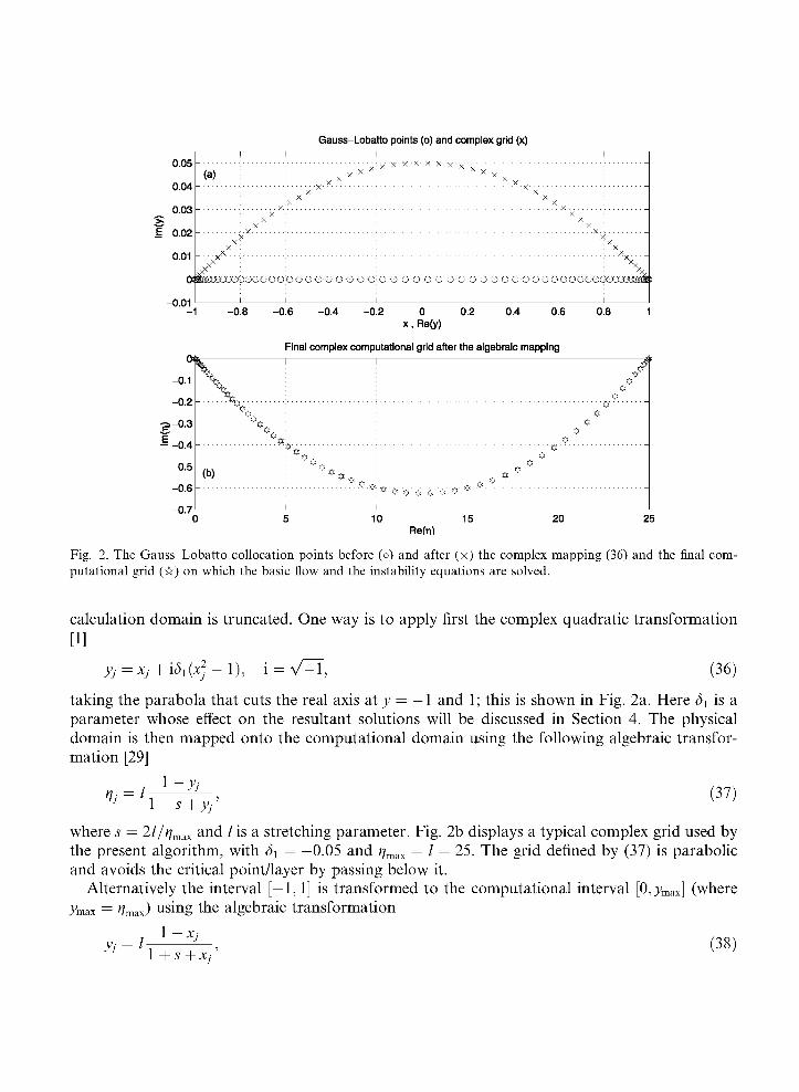
Fig. 2. The Gauss-Lobatto collocation points before (o) and after (x) the complex mapping (36) and the final com­putational grid (-&) on which the basic flow and the instability equations are solved.

calculation domain is truncated. One way is to apply first the complex quadratic transformation [1]

y¡ =xj + iS1(x2j - 1), i (36)

taking the parábola that cuts the real axis at y = — 1 and 1; this is shown in Fig. 2a. Here ¿h is a parameter whose effect on the resultant solutions will be discussed in Section 4. The physical domain is then mapped onto the computational domain using the following algebraic transfor­mation [29]

1-yj r¡j = l- (37)

1+s + yj'

where s = 21/r¡max and / is a stretching parameter. Fig. 2b displays a typical complex grid used by the present algorithm, with ¿h = —0.05 and r¡max = 1 = 25. The grid defined by (37) is parabolic and avoids the critical point/layer by passing below it.

Alternatively the interval [—1,1] is transformed to the computational interval [0, jmax] (where ) using the algebraic transformation

1 — Xj y} = l

1 + S + Xj ' (38)

and then mapped onto the complex domain, passing through the real points r¡ = 0, r¡ = t]max, using

f/ • = y¡ + ic2

fmax (39)

where m is an integer with m ^ 2 and c2 is a parameter, both of which determine the character-istics of the integration path; as m increases (assuming that c2 < 0 and remains constant) the máximum depth of the complex integration path increases and its mínimum shifts towards the Re(r¡) = 0 axis, thus enabling the handling of critical points/layers which lie cióse to r¡ = 0. This is useful in calculations of inviscid instability of incompressible wall-bounded flows. On the other hand, by changing the sign of c2, one can intégrate above or below the real axis, for c2 > 0 or c2 < 0, respectively. Further, by increasing the absolute valué of c2 one can increase the máximum depth/height of the complex integration path. Note, the real parts of the complex-grid points (37) and (39) constructed using these altérnate approaches are not identical. In other words, the real grid generated by setting 5\ = 0 is not the same as the one obtained for c2 = 0.

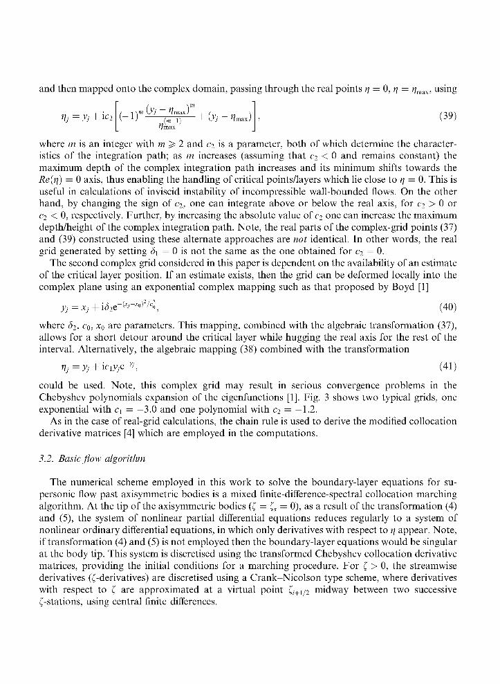
The second complex grid considered in this paper is dependent on the availability of an estímate of the critical layer position. If an estímate exists, then the grid can be deformed locally into the complex plañe using an exponential complex mapping such as that proposed by Boyd [1]

yj=Xj + i52e-{xj-Xo)2/c\ (40)

where S2, c0, x0 are parameters. This mapping, combined with the algebraic transformation (37), allows for a short detour around the critical layer while hugging the real axis for the rest of the interval. Alternatively, the algebraic mapping (38) combined with the transformation

r¡j = yj + iciyjer», (41)

could be used. Note, this complex grid may result in serious convergence problems in the Chebyshev polynomials expansión of the eigenfunctions [1]. Fig. 3 shows two typical grids, one exponential with c\ = —3.0 and one polynomial with c2 = —1.2.

As in the case of real-grid calculations, the chain rule is used to derive the modified collocation derivative matrices [4] which are employed in the computations.

3.2. Basic flow algorithm

The numerical scheme employed in this work to solve the boundary-layer equations for su-personic flow past axisymmetric bodies is a mixed finite-difference-spectral collocation marching algorithm. At the tip of the axisymmetric bodies (£ = £* = 0), as a result of the transformation (4) and (5), the system of nonlinear partial differential equations reduces regularly to a system of nonlinear ordinary differential equations, in which only derivatives with respect to r¡ appear. Note, if transformation (4) and (5) is not employed then the boundary-layer equations would be singular at the body tip. This system is discretised using the transformed Chebyshev collocation derivative matrices, providing the initial conditions for a marching procedure. For £ > 0, the streamwise derivatives (C-derivatives) are discretised using a Crank-Nicolson type scheme, where derivatives with respect to t, are approximated at a virtual point £¡+i/2 midway between two successive C-stations, using central finite differences.

-0.5

* i ítt *

O * o *

- o -* o * » * * o

± o * o * í o * o

o o o o o o o o o o

\ o o Polynomial * * Exponential

10 15 20 25

I r

30 35 40 45 50

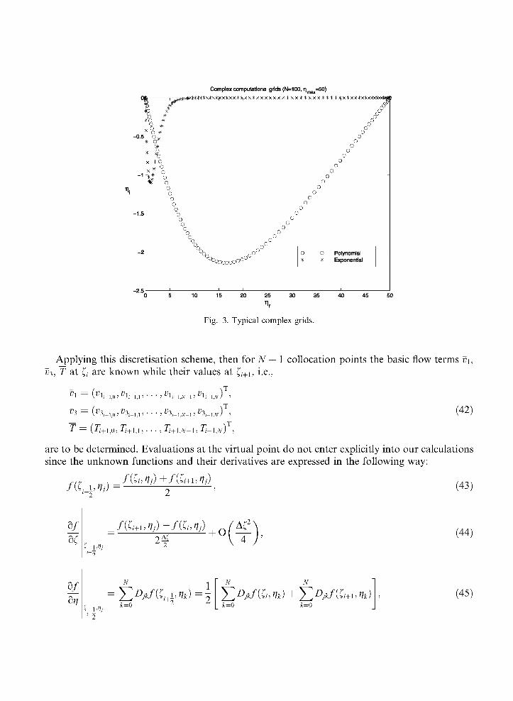
Fig. 3. Typical complex grids.

Applying this discretisation scheme, then for N + 1 collocation points the basic flow terms v\, V3, T at C¿ are known while their valúes at £¡+i, Le.,

vl = K + i . o ^ l m . n - ' - ^ U . vh-l¡+l,iV-l ' " íi+lfl ) '

«3 = (i>3i+li„ , i > 3 i + M , . . . , Ü3 ¡ + 1 ; W_ 1 , Vi¡+l¡N ) , (42)

^ — (7¿+i,0) 7¿+i,i) • • •) T¡+\,N-\, Ti+\r N

are to be determined. Evaluations at the virtual point do not enter explicitly into our calculations since the unknown functions and their derivatives are expressed in the following way:

_f{íun])+f{íi+un]) ñC^nj) (43)

8C i + 2

^ 2 + o 4

(44)

^Djknci+L,m) t. í'ij

k=0 ¿D,i/(C¿,í7i) + ¿^/(U,%) k=0 k=0

(45)

where/is one of v>\, ü3 or T. Thus, in the resultant discrete nonlinear system 3 (TV + 1) unknowns appear, i.e., the valúes of the three unknowns v>\, ü3, T at the (TV + 1) grid points, while the co-efficients of these equations contain the known valúes of these quantities at the previous C-station, £¡. In this way, at each streamwise station £¿+1 (for £ > 0), a 3 (TV + 1) x 3 (TV + 1) complex non-linear algebraic system is formed. The real and imaginary parts of this system are separated yielding a 6(/V + 1) x6(7V+l) nonlinear real algebraic system which is then solved using Broy-den's and/or Newton's methods. In the present study, since the dimensión of the nonlinear system is rather low (typical valúes range from 192 x 192 to 384 x 384) use of preconditioning may be circumvented. We will return to this issue in more detail later.

Compared with the solution approach of Pruett and Streett [25] ours is algorithmically simpler but their scheme discretises the C-derivatives with fifth-order accuracy as opposed to the second-order accuracy that our scheme provides. However, since the type of boundary-layer flow we consider evolves slowly in the downstream spatial direction and we concéntrate our instability analysis on the región cióse to the leading edge, which previous studies have shown to be the most important in the context of linear instability analysis from a physical point of view, it was not felt that a scheme of higher formal order of accuracy in the streamwise direction was necessary. Another difference between the algorithm of Pruett and Streett [25] and our scheme, is that ours solves the boundary-layer equations directly in the complex r¡ plañe; on the other hand, the techniques described herein could be combined with the scheme of [25] without conceptual dif-ficulties. It should be clear that in choosing the outlined simple approach for the solution of the basic flow problem we did not aim at improving efficiency in comparison with the work of [25]; rather, our intention has been to design an adequate and simple algorithm which is capable of providing reliable solutions of the basic flow problem for the subsequent instability analysis. The characteristics of the algorithm from the point of view of both accuracy and efficiency will be examined in what follows.

3.3. Inviscid instability algorithms

Methods for the determination of the eigenvalues of the inviscid linear instability equations can be divided into two classes—global or local. In a global calculation the eigenvalue problem is written as a matrix eigenvalue problem whose full spectrum is then calculated, typically using the QZ algorithm [13]. However, on account of the memory and corresponding CPU time require-ments scaling with the square and the cube of the leading dimensión of the matrix, respectively, global methods are often replaced by local methods where the focus is on the calculation of a single eigenvalue. Care has to be exercised here in the interpretation of the term 'local', which is also used in the context of the method utilised for the numerical calculation of derivatives. Within the framework of a local algorithm for the recovery of the eigenvalue one may use 'local' finite-diflerence based shooting algorithms, such as Runge-Kutta or Adams-Bashforth schemes, to calcúlate the eigenvalue. This was not done in the present work, but we rather use a 'global' spectral method to set up the matrix eigenvalue problem. The advantage of local methods for the calculation of the eigenspectrum is that all one's computing resources may be devoted to the resolution of a single eigenvalue/eigenvector pair. However, there is a need for a reasonably ac-curate initial guess. Both methods are described in what follows; in practice a combination of both

is used with a global solution providing an estímate of the eigenvalue which is subsequently re-fined by a local search.

As was discussed in the introduction a major difficulty faced in conducting inviscid instability calculations is how to treat the critical layer región [31]. Since most of the eigenvalues correspond to growing/decaying (Im(/? ^ 0)) disturbances a singularity will not explicitly exist in the critical layer, but strong gradients do cause solution problems. Finer grids in the neighbourhood of the critical layer might be one solution but this increases computational cost substantially on account of the dense spectral matrices introduced. As has been mentioned, the method we employ to alleviate the strong gradients problem is the use of complex grids, Le., we solve the instability equations directly in complex space away from the strong gradients. This however presents a different problem in that how do we obtain the relevant basic flow velocity and temperature profiles at the complex-grid points? A common practice, which has been used by many investi-gators is the extensión of the real basic flow profiles into the complex plañe by means of truncated Taylor series expansions. This technique has been successfully adopted for both local shooting (for example, [6,8,19]) and global spectral [9,10] schemes. For example, to determine the valid streamwise basic flow velocity valué Wo at the complex-grid point r¡ = r¡r + ir¡¡ one would evalúate

WM = w,{nr) + if/Xfo) - 1 <(f/,) - i | <'(f/,) +1- <"(f/,) + otó). (46)

Clearly the accuracy of this approach is dependent on the truncation error and for the problem considered here effects the accuracy of the instability calculations (see Section 4.1.2). The existence of an alternative scheme can assist in assessing the accuracy and efficiency of the Taylor-expansion approach. The alternative we consider in this work is to solve the basic flow (boundary layer) equations in the í,-direction directly in the complex plañe using the same grids as those used for the subsequent instability analysis [16].

3.3.1. Global algorithm for the entire eigenspectrum The global algorithm which we employ in order to derive an approximation of the entire

spectrum of eigenvalues is the standard QZ scheme. In order to formúlate a generalised eigenvalue problem the inhomogeneous far-field boundary condition (27) was replaced by a homogeneous boundary condition, Le., p(r¡max) = 0 or by the asymptotic boundary condition p' + cp = 0 at r¡ = r\m¡ÍX. Alternative boundary conditions will be presented in what follows in this section; their effect on the accuracy of the instability calculations will be examined in Section 4.3.3. In this work we only present (and consider) the spatial versión of the QZ algorithm, although there is no conceptual problem in deriving the analogous temporal matrix system. As a first step, Eq. (25) is written in the following form:

d , ,_ d2 , , 2 ft«2c2ro , cor0c d a)T0n- + a)T0 — + aSM^ — +

úv] ÚY}¿ úv] r úr¡

P dr¡ dr¡2 °° r2 r dr¡ 2

W0T0„i- + W0T0i^-2W0„T0i- + ^ ^ i- + 3W0M2m

d , „ r r r d 2 ,7TA „, d , ÍT0W0 d , „ 7 T _ 2 2 n2ÍT0W0 P

+ a2 [- 3 W02Mloj + ojT0]p + a3 [M¿ W¡ - T0 W0]p, (47)

where r = 1 +1£2 + £r¡. Then, the companion matrix approach of Bridges and Morris [3] is em-ployed; using the appropriate collocation derivative matrices the above eigenvalue problem is approximated by a nonlinear algebraic eigenvalue problem of the form

EX = txFX + tx2GX + a.3 HX, (48)

where X = \p0,p1:... ,pN] are the valúes of the pressure eigenfunction at the collocation points (Le., pj =p(r¡j) for j = 0,... ,N). The nonzero entries of the matrices E, F, G, H are given in Appendix A. The above (TV + 1) x (TV + 1) nonlinear eigenvalue problem is then converted to the following 3 (TV + 1) x 3 (TV + 1) linear eigenvalue problem:

BY = aCY, (49)

where

B E 0 0

0 I 0

0~ 0 I

, c = F G H~ I O O O I O

, Y = ' X '

aX éX

(50)

while / is the unitary and O the zero matrix. Finally, the QZ algorithm is employed to solve the eigenvalue problem (49) for a.

3.3.2. Iterative algorithm for a single eigenvalue In order to use the iterative algorithm at a given streamwise position £¿ Eqs. (20) and (21) are

discretised at the (TV + 1) spectral collocation grid points yielding a linear inhomogeneous alge­braic system which can be expressed in the form

AX Ax A,

A2

A4 (51)

where q> = (q>0, q>\,..., q>N) , p = {Po,p\, • • • ,pN) • The elements of the submatrices Ai, A2, A3, A4

and the vector b are given in Appendix B. The Nth and 2/Vth lines of matrix A are reserved for the boundary conditions. All but two elements of the vector b are zero. The nonzero elements appear at the Nth and 2/Vth positions corresponding to the asymptotic valúes of cp and p at the far-field position r¡max, Le., conditions (23) and (24).

Starting with a suitable initial guess of the required eigenvalue, the algebraic system (51) is solved iteratively, by means of a Newton-iteration scheme [19], until the impermeability condition on the surface (Le., (p(0) = 0) is satisfied. The above described scheme is able to perform temporal as well as spatial instability calculations giving spectrally accurate results at the same level of computing effort. A similar iterative scheme was proposed by Malik [22] for the solution of viscous, compressible instability equations on a real grid. Standard numerical library subroutines were used for the solution of the linear system (51) and the evaluation of the modified Bessel functions.

3.3.3. Far-field boundary conditions Finally we discuss the boundary conditions closing the inviscid linear instability equations,

which determine the strategy used for the recovery of the most interesting unstable/least damped eigenvalues; if the latter appear nonlinearly in the boundary conditions the iterative algorithm

must be used, otherwise either the local or the global procedure for the recovery of the eigen-spectrum may be applied. Boundary conditions considered in this work are:

(a) Asymptotic (inhomogeneous): The instability equations are used in the form (20) and (21) combined with the asymptotic valúes for the disturbance amplitudes (23) and (24) in the far field. The discrete system is inhomogeneous, so the iterative spectral technique, as described in Section 3.3.2, is employed.

(b) Homogeneous: The instability problem is described by Eq. (25) and homogeneous far-field conditions are imposed; setting/5 (0) = 0, a nonlinear generalised eigenvalué problem as described in Section 3.3.1 may be formulated. The far-field boundary conditions are

/K>Wx) = 0. (52)

(c) Homogeneous far-field-normalized pressure: The instability equations are used in the form (20) and (21) but the far-field asymptotic conditions are discarded. Instead of the homogeneous boundary condition on the pressure derivative at the wall ¿5(0) = constant is imposed and, further, this constant is taken to be equal to unity. This assumption is equivalent to a normalization of the eigenfunctions by the valué of pressure amplitude on the solid surface (r¡ = 0). Thus, the boundary conditions now read

¿5(0) = 1, <KVax)=0. (53)

The discrete system (51) remains inhomogeneous and the spectral iterative technique described in Section 3.3.2 can also be used here. One only needs to redefine vector b in Eq. (51), which now becomes¿ = (0,0, . . . ,0,0,1)T .

4. Results

We now turn to the presentation of the results obtained by application of the algorithms discussed in the previous section. The effect of a critical layer location which progressively moves away from the solid wall is examined by focusing first on incompressible flow on flat-plate ge-ometries, where critical layers form in the immediate vicinity of the wall, and then proceeding to the study of compressible flow over both planar and axisymmetric configurations, in both of which critical layers are present in the neighbourhood of the respective free-streams. Owing to the numerical nature of this work parametric studies are confined to those parameters related to the complex mappings which form the central theme of this paper. The remaining physical parameters were chosen to match those of the respective established works against which we compare our predictions.

4.1. Basic flow

In this section we ascertain the capability of the proposed coupled finite-difference/spectral collocation scheme to obtain accurate solutions to the compressible boundary-layer equations (6)-(8). We assess the efficiency of the spectral methods in which dense matrices must be inverted at each streamwise location against the standard finite-difference scheme in which a much larger number of nodes is required to obtain the same order of accuracy, but sparse matrices are being

inverted. Within spectral computations, we quantify the overheads incurred by the complex-grid algorithm and, finally, we compare basic flow results obtained by spectral solutions in the complex plañe against those delivered by Taylor-expansion of profiles obtained on a real spectral collo­cation grid.

4.1.1. Direct solution in the complex plañe As a part of the validation process we first compare the numerically determined streamwise

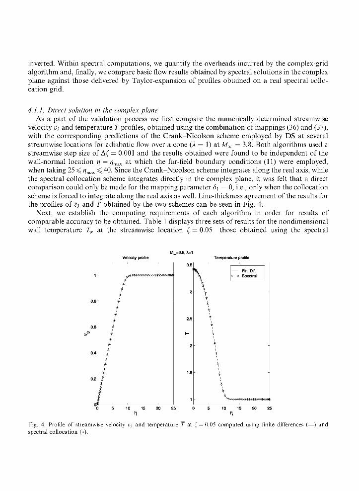
velocity Ü3 and temperature T profiles, obtained using the combination of mappings (36) and (37), with the corresponding predictions of the Crank-Nicolson scheme employed by DS at several streamwise locations for adiabatic flow over a cone (1 = 1) at Mx = 3.8. Both algorithms used a streamwise step size of A£ = 0.001 and the results obtained were found to be independent of the wall-normal location r¡ = r¡max at which the far-field boundary conditions (11) were employed, when taking 25 ^ r¡max ^ 40. Since the Crank-Nicolson scheme integrates along the real axis, while the spectral collocation scheme integrates directly in the complex plañe, it was felt that a direct comparison could only be made for the mapping parameter Si = 0, Le., only when the collocation scheme is forced to intégrate along the real axis as well. Line-thickness agreement of the results for the profiles of ü3 and T obtained by the two schemes can be seen in Fig. 4.

Next, we establish the computing requirements of each algorithm in order for results of comparable accuracy to be obtained. Table 1 displays three sets of results for the nondimensional wall temperature Tw at the streamwise location £ = 0.05—those obtained using the spectral

M =3.8, *=1 Velocity profile Temperature profile

Fig. 4. Profile of streamwise velocity v3 and temperature T at ( — 0.05 computed using finite differences (—) and spectral collocation (*).

Table 1 Adiabatic boundary-layer flow on a cone (1 — 1) at M^ = 3.8

Spectral methods

Real grid

N Tv

32 3.372683 48 3.372180 64 3.372164 80 3.372164 96 3.372164

CPU time

Total

(s) 16 51

122 237 417

/Iter/node (ms)

0.5 1.0 1.4 2.2 3.1

Complex

Tv

3.373363 3.372250 3.372170 3.372164 3.372163

grid

CPU time

Total

(s) 116 401 919

1726 2946

/Iter/node (ms)

1.2 2.5 4.8 6.5 8.9

Finite-difference method

N

501 1001 2001 4001 8001

Tv

3.372118 3.372152 3.372160 3.372162 3.372163

CPU ti

Total

(s) 61

122 246 529

1153

me

/Iter/node (LJS)

43 43 43 46 50

Basic flow results for the temperature at the wall (rw) at f — 0.05 and respective timings as a function of the number iV of collocation points used in real (¿i — 0) and complex (¿i — —0.05) grid spectral calculations and of the number of nodes iV used in the Crank-Nicolson finite-difference calculations, respectively. A( — 10~3.

method using S\ = 0 and S = —0.05 alongside results obtained using the Crank-Nicolson scheme. For a fair comparison to be made, the number of collocation points used in the spectral calcu­lations and that of the nodes on which the finite-difference algorithm was set up were chosen so as to deliver results of comparable accuracy for Tw. Basic flow timings were obtained on a work-station and the conclusions which may be drawn from these results are the following. Firstly, the finite-difference and both spectral algorithms predict the same converged results for the param-eters chosen, a result which was confirmed to hold for all the parameter valúes examined. This holds for the results delivered by the two spectral calculations, pointing at the independence at convergence of the spectral predictions on the complex-grid parameter mappings chosen in these runs. Secondly, the number of discretisation points used by the complex-grid spectral and the finite-difference schemes is similar to known comparisons of real-grid spectral and finite-difference viscous linear instability calculations [17]; typically, an order of magnitude larger number of points is required by the latter in order for the accuracy of the former scheme to be met. Thirdly, from the point of view of efficiency several points are highlighted by the total CPU time consumed by the algorithms examined.

Focusing on the two real-grid calculations, it is interesting to note that the advantage offered by the superior convergence properties of the spectral scheme over the finite-difference algorithm at the same level of discretisation is not offset by the inversión of sparse matrices in the latter as opposed to the dense matrices required by the former scheme; in addition to requiring less memory, the real-grid spectral algorithm is over a factor two faster than its finite-difference counterpart. On the other hand, obtaining the basic flow solution on the complex grid is the most computationally intensive of the three algorithms. However, one should note that the solution on the complex grid can be used directly in the subsequent instability analysis, while the real-grid solutions need to be transferred onto a complex grid by Taylor-expansion, as will be discussed in the next section. In view of the additional overhead that the latter procedure requires, obtaining the basic flow directly on a complex grid becomes a competitive alternative from the point of view of efficiency also.

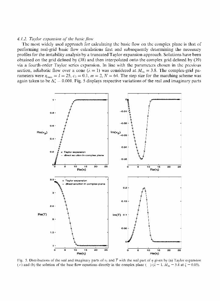
4.1.2. Taylor expansión of the basicflow The most widely used approach for calculating the basic flow on the complex plañe is that of

performing real-grid basic flow calculations first and subsequently determining the necessary profiles for the instability analysis by a truncated Taylor expansión approach. Solutions have been obtained on the grid defined by (38) and then interpolated onto the complex grid defined by (39) via a fourth-order Taylor series expansión. In line with the parameters chosen in the previous section, adiabatic flow over a cone (1 = 1) was considered at Mx = 3.8. The complex-grid pa­rameters were r¡max = 1 = 25, c2 = 0.1, m = 2, N = 64. The step size for the marching scheme was again taken to be A£ = 0.001. Fig. 5 displays respective variations of the real and imaginary parts

Re(v3)

Re(T)

;XXXXX>OOOO»«HI

x T a y l o r e x p a n s i ó n

— d i r e c t s o l u t i o n in c o m p l e x p l a ñ e

lm(v3)

10 15 20 25 Re(n)

x Taylor expansión

direct solution In complex plañe

00000(M>00000000<H>*«M

l m ( T ) 0.1

5 10 15 20 25

Re(n)

Fig. 5. Distributions of the real and imaginary parts of v3 and T with the real part of t¡ given by (a) Taylor expansión (x) and (b) the solution of the base flow equations directly in the complex plañe (—) (1 — 1, M^ — 3.8 at ( — 0.05).

of velocity and temperature profiles with the real part oí r¡ at £ = 0.05. For the complex streamwise velocity profiles agreement was obtained to the second decimal place for the real parts and the third decimal place for the imaginary parts, while a larger deviation was observed for the temperature profiles, with agreement to the first and second decimal places having been obtained for the real and the imaginary parts of this quantity for the same parameters. This level of ac-curacy of the Taylor-expanded basic flow in comparison to that obtained directly on the complex grid is to be expected for the parameters chosen since the complex grid has max(j7¿) ~ —0.6 which results in a máximum truncation error 0(max(t]¡) ) ~ — 8 x 10~2. We will return to this issue when we present our instability results.

Summarising our basic flow calculations, we have demonstrated that accurate results may be obtained by spectral methods on either real or complex collocation grids, in line with the analogous result of Pruett and Streett [25] obtained on real collocation grids. Results agreeing reasonably well with each other have been obtained either directly on the complex plañe or interpolated from real-grid calculations using a Taylor series expansión. The adequacy of either approach from the point of view of accuracy will be quantified shortly by reference to the eigenvalue problem results. Re-garding efficiency, both spectral timings may be improved by use of preconditioning; this is beyond the scope of the present work, the objective of which is provisión of basic flow quantities for the instability analyses, and could be undertaken as an extensión of the present work.

4.2. Incompressible inviscid linear instability

We commence with the presentation of the linear instability results by considering the classic Rayleigh equation which, despite its apparent simplicity, provides a good test for our proposed algorithms due to the fact that for incompressible boundary-layer flows the critical layer is typ-ically located very cióse to the wall. The complex grids which we employ need to coincide with the real point on the fixed boundary, where the boundary conditions are applied. Thus the compu-tational grid must be deviated around the critical layer an extremely short distance away from the boundary. In the case of Sturm-Liouville eigenproblems of the fourth kind and certain kinds of barotropic instability problems [1,11] this was achieved by considering nonzero imaginary parts for the complex mapping parameters (Si,S2,ci,C2) or, additionally, by applying composite complex maps, as proposed by Gilí and Sneddon [12]. Gilí and Sneddon also provide explicit formulae for the calculation of the optimal valúes for the complex mapping parameters which depend on the location of the critical point [11]. For the problem at hand, the optimal complex grid given by the formulae of Gilí and Sneddon was found to cause serious convergence problems and degraded the accuracy of the basic flow calculations. If such a grid were to be used, the basic flow and the instability equations must be solved on different grids.

Here we have chosen to solve the boundary-layer equations directly on the complex plañe and use the same grid for the instability calculations. Although this is not the optimal grid in the sense of Gilí and Sneddon [11], it offers accuracy and robustness as will be shown next. In what follows we use two sets of complex mappings resulting from a combination of (38) with either (39) or (41), both of which have the ability to divert the complex grid over short distances. The test cases considered are two model inviscid linear instability problems, that of the Blasius boundary layer [19] and a modified asymptotic suction pro file [24]. Both problems share the characteristic of critical layer location cióse to the solid wall.

4.2.1. The Blasius boundary layer The basic flow pro file Wü{r\) was obtained by solving the Blasius equation on a real grid (i.e,

c2 = 0 or c\ = 0) or directly on a complex grid. If the former case, a Taylor expansión along the lines of Section 3.3 was used to calcúlate the valúes of W(r¡) on the complex nodes. The Rayleigh equation was discretised on the complex grid resulting from the combination of (38) and (39) or (38) and (41), using the appropriate collocation derivative matrices. The discrete eigenvalue problem was thus formulated as a generalised eigenvalue problem which was solved using the QZ algorithm.

In order to study the accuracy and efficiency of the proposed algorithm we compare our results to those of Mack [19] (Table 3.1, p. 3-16) who computed eigenvalues with an indented integration contour. For a = 0.179 Mack quotes the eigenvalue co = 0.05750554 — iO.00657109 while the present spectral method yields co = 0.05750493 — iO.00657192 when the exponential mapping with c\ = —3.0 is employed, and co = 0.05750493 — iO.00657191 when the polynomial mapping with C2 = —0.15, m = 5 is used. For both spectral method calculations 100 collocation points were used with r¡max = / = 50. The effect of varying the complex mapping parameters c\ and C2 on the re-sultant accuracy of the inviscid eigenvalue for the wavenumbers a = 0.128 and 0.180 is shown in Table 2. In this table we also compare eigenvalues calculated using a basic flow determined by Taylor expansión of the Blasius solution into the complex plañe (case I) against the case where the Blasius equation is solved directly in the complex plañe (case II). The conclusión which may be drawn from these results is that case II calculations are more robust, with results depending more weakly on the complex-mapping parameter valúes than those in the case I calculations; this conclusión holds for both exponential and algebraic mappings. In Table 3 we keep the complex-grid mapping parameters fixed and vary the number of collocation points. Exponential

Table 2 Dependence of the eigenvalue on the exponential and the polynomial mapping parameters, for the case of the Blasius boundary layer using N — 100 collocation points (m — 5, t¡m¡¡x — l — 50)

C\

Exponential mapping -0.5 -2.0 -3.0 -4.0

Polynomial mapping -0.05 -0.08 -0.12 -0.15

[19]

co

Case Ia

a = 0.12*

0.03327 -0.03328 -0.03325 -0.03322 -

0.03323 -0.03329 -0.03326 -0.03323 -

0.0333 -

i

- iO.00228 - iO.00231 - iO.00237 - iO.00246

- iO.00224 - iO.00228 - iO.00230 - iO.00235

iO.00233

a = 0.180

0.05683 -0.05802 -0.05801 -0.05800 -

0.05695 -0.05798 -0.05793 -0.05786 -

0.0580 -

- iO.00672 - iO.00674 - iO.00687 - iO.00707

- iO.00679 - iO.00667 - iO.00671 - iO.00685

iO.00680

Case IIb

a = 0.128

0.03330 -0.03329 -0.03329 -0.03329 -

0.03334-0.03329 -0.03329 -0.03329 -

- iO.00229 - iO.00229 - iO.00229 - iO.00229

- iO.00234 - iO.00229 - iO.00229 - iO.00229

a = 0.180

0.05809 -0.05801 -0.05801 -0.05801 -

0.05830-0.05802-0.05801 -0.05801 -

iO.00615 iO.00668 iO.00668 iO.00668

iO.00621 iO.00668 iO.00668 iO.00668

a Using Taylor expansión for the calculation of the base flow profile in the complex plañe. b Solving the Blasius equation directly in the complex plañe.

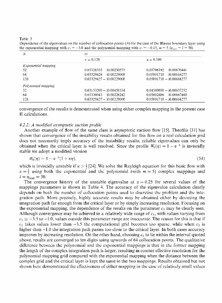
Table 3 Dependence of the eigenvalues on the number of collocation points (N) for the case of the Blasius boundary layer using the exponential mapping with c\ — —3.0 and the polynomial mapping with c2 — —0.15, m — 5 (f?max — l — 50)

N (o

a = 0.128 a = 0.1É

Expone) 32 64 128

Polynor, 32 64 128

ntial mapping

nial mapping

0.03326355 -0.03329428 -0.03329427 -

0.03153209-0.03330043 -0.03329427 -

- iO.00230571 - iO.00229008 - iO.00229008

- iO.00458334 - iO.00228242 - iO.00229008

0.05798192 - iO.00670441 0.05801718-iO.00668277 0.05801718-iO.00668277

0.04369888 - iO.00637252 0.05802486 - iO.00667460 0.05801718-iO.00668277

convergence of the results is demonstrated when using either complex mapping in the present case II calculations.

4.2.2. A modified asymptotic suction profile Another example of flow of the same class is asymptotic suction flow [15]. Theofilis [31] has

shown that convergence of the instability results obtained for this flow on a real calculation grid does not necessarily imply accuracy of the instability results; reliable eigenvalues can only be obtained when the critical layer is well resolved. Since the profile Wo(r¡) = 1 — e~*> is inviscidly stable we adopt a modified versión

W0{ri) = l-e-'>{l+Kri), (54)

which is inviscidly unstable if K > \ [24]. We solve the Rayleigh equation for this basic flow with K = \ using both the exponential and the polynomial (with m = 5) complex mappings and / = V a x = 30.

The convergence history of the unstable eigenvalué at a = 0.25 for several valúes of the mappings parameters is shown in Table 4. The accuracy of the eigenvalue calculation clearly depends on both the number of collocation points used to discretise the problem and the inte-gration path. More precisely, highly accurate results may be obtained either by deviating the integration path far enough from the critical layer or by simply increasing resolution. Focusing on the exponential mapping, the dependence of the results on the parameter c\ may be clearly seen. Although convergence may be achieved in a relatively wide range of c\, with valúes varying from c\ ~ —3.5 to -1.0, valúes outside this parameter range are inaccurate. The reason for this is that if c\ takes valúes lower than -3.5 the computational grid becomes too sparse, while when c\ is higher than -1.0 the integration path passes too cióse to the critical layer. In both cases accuracy improves by increasing resolution. On the other hand, choosing c\ to lie within the interval quoted above, results are converged to ten digits using upwards of 64 collocation points. The qualitative difference between the polynomial and the exponential mappings is that in the former mapping the length of the complex integration path is larger, resulting in coarser effective resolution for the polynomial mapping grid compared with the exponential mapping when the distance between the complex grid and the critical layer is kept the same in the two mappings. Results obtained but not shown here demonstrated the effectiveness of either mapping in the case of relatively small valúes

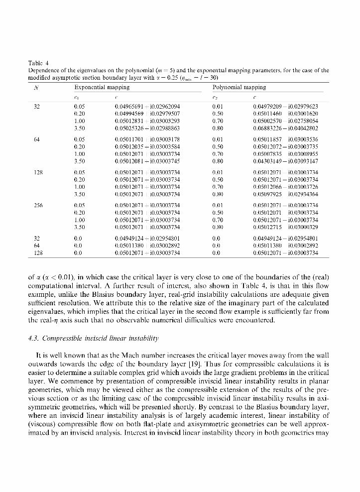
Table 4 Dependence of the eigenvalues on the polynomial (m • modified asymptotic suction boundary layer with a =

- 5) and the exponential mapping parameters, for the case of the 0.25 ( ^ = / = 30)

N

32

64

128

256

32 64 128

Exponential

0.05 0.20 1.00 3.50

0.05 0.20 1.00 3.50

0.05 0.20 1.00 3.50

0.05 0.20 1.00 3.50

0.0 0.0 0.0

mapping

c

0.04965691+Í0.02962094 0.04994569+ Í0.02979507 0.05012831+Í0.03003293 0.05025326+ Í0.02988863

0.05011701+Í0.03003178 0.05012035+ Í0.03003584 0.05012071 +Í0.03003734 0.05012081+Í0.03003745

0.05012071 +Í0.03003734 0.05012071 +Í0.03003734 0.05012071 +Í0.03003734 0.05012071 +Í0.03003734

0.05012071 +Í0.03003734 0.05012071 +Í0.03003734 0.05012071 +Í0.03003734 0.05012071 +Í0.03003734

0.04949124+ Í0.02954801 0.05011380+ Í0.03002892 0.05012071 +Í0.03003734

Polynomial

0.01 0.50 0.70 0.80

0.01 0.50 0.70 0.80

0.01 0.50 0.70 0.80

0.01 0.50 0.70 0.80

0.0 0.0 0.0

mapping

c

0.04979209+ Í0.02979623 0.05011460 + Í0.03001620 0.05002570+ Í0.02758054 0.06883226+ Í0.04042802

0.05011857 + Í0.03003536 0.05012072+ Í0.03003735 0.05007835+ Í0.03008955 0.04303149+ Í0.03093147

0.05012071 +Í0.03003734 0.05012071 +Í0.03003734 0.05012066+ Í0.03003726 0.05097925+ Í0.02934364

0.05012071 +Í0.03003734 0.05012071 +Í0.03003734 0.05012071 +Í0.03003734 0.05012715+ Í0.03000329

0.04949124+ Í0.02954801 0.05011380 + Í0.03002892 0.05012071 +Í0.03003734

of a (a < 0.01), in which case the critical layer is very cióse to one of the boundaries of the (real) computational interval. A further result of interest, also shown in Table 4, is that in this flow example, unlike the Blasius boundary layer, real-grid instability calculations are adequate given sufficient resolution. We attribute this to the relative size of the imaginary part of the calculated eigenvalues, which implies that the critical layer in the second flow example is sufficiently far from the real-?? axis such that no observable numerical difficulties were encountered.

4.3. Compressible inviscid linear instability

It is well known that as the Mach number increases the critical layer moves away from the wall outwards towards the edge of the boundary layer [19]. Thus for compressible calculations it is easier to determine a suitable complex grid which avoids the large gradient problems in the critical layer. We commence by presentation of compressible inviscid linear instability results in planar geometries, which may be viewed either as the compressible extensión of the results of the pre-vious section or as the limiting case of the compressible inviscid linear instability results in axi-symmetric geometries, which will be presented shortly. By contrast to the Blasius boundary layer, where an inviscid linear instability analysis is of largely academic interest, linear instability of (viscous) compressible flow on both flat-plate and axisymmetric geometries can be well approx-imated by an inviscid analysis. Interest in inviscid linear instability theory in both geometries may

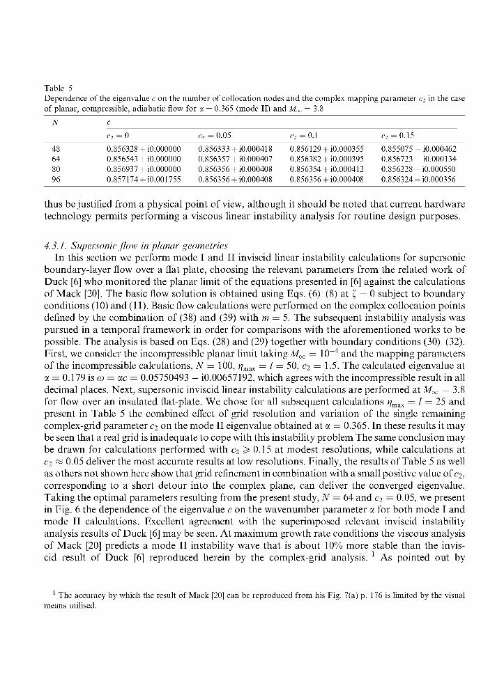
Table 5 Dependence of the eigenvalue c on the number of collocation nodes and the complex mapping parameter c2 in the case of planar, compressible, adiabatic flow for a — 0.365 (mode II) and M^ — 3.8

N

48 64 80 96

c

c2 = 0

0.856328+ Í0.000000 0.856543+ Í0.000000 0.856937+ Í0.000000 0.857174+ Í0.001755

c2 = 0.05

0.856333+ Í0.000418 0.856357+ Í0.000407 0.856356+ Í0.000408 0.856356+ Í0.000408

c2 = 0.1

0.856129+ Í0.000355 0.856382+ Í0.000395 0.856354+ Í0.000412 0.856356+ Í0.000408

c2 = 0.15

0.855075 - iO.000462 0.856723 - iO.000134 0.856228+ Í0.000550 0.856324+ Í0.000356

thus be justified from a physical point of view, although it should be noted that current hardware technology permits performing a viscous linear instability analysis for routine design purposes.

4.3.1. Supersonic flow in planar geometries In this section we perform mode I and II inviscid linear instability calculations for supersonic

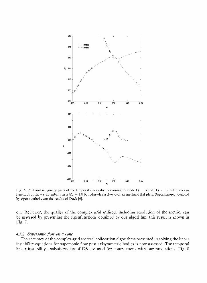
boundary-layer flow over a flat píate, choosing the relevant parameters from the related work of Duck [6] who monitored the planar limit of the equations presented in [6] against the calculations of Mack [20]. The basic flow solution is obtained using Eqs. (6)-(8) at t, = 0 subject to boundary conditions (10) and (11). Basic flow calculations were performed on the complex collocation points defined by the combination of (38) and (39) with m = 5. The subsequent instability analysis was pursued in a temporal framework in order for comparisons with the aforementioned works to be possible. The analysis is based on Eqs. (28) and (29) together with boundary conditions (30)-(32). First, we consider the incompressible planar limit taking M^ = 10~4 and the mapping parameters of the incompressible calculations, N = 100, r¡max = 1 = 50, c2 = 1.5. The calculated eigenvalue at a = 0.179 is co = ac = 0.05750493 — iO.00657192, which agrees with the incompressible result in all decimal places. Next, supersonic inviscid linear instability calculations are performed atMoo = 3.8 for flow over an insulated flat-plate. We chose for all subsequent calculations r¡max = / = 25 and present in Table 5 the combined effect of grid resolution and variation of the single remaining complex-grid parameter c2 on the mode II eigenvalue obtained at a = 0.365. In these results it may be seen that a real grid is inadequate to cope with this instability problem The same conclusión may be drawn for calculations performed with c2 5* 0.15 at modest resolutions, while calculations at c2 « 0.05 deliver the most accurate results at low resolutions. Finally, the results of Table 5 as well as others not shown here show that grid refinement in combination with a small positive valué of c2, corresponding to a short detour into the complex plañe, can deliver the converged eigenvalue. Taking the optimal parameters resulting from the present study, N = 64 and c2 = 0.05, we present in Fig. 6 the dependence of the eigenvalue c on the wavenumber parameter a for both mode I and mode II calculations. Excellent agreement with the superimposed relevant inviscid instability analysis results of Duck [6] may be seen. At máximum growth rate conditions the viscous analysis of Mack [20] predicts a mode II instability wave that is about 10% more stable than the invis­cid result of Duck [6] reproduced herein by the complex-grid analysis. l As pointed out by

1 The accuracy by which the result of Mack [20] can be reproduced from his Fig. 7(a) p. 176 is limited by the visual means utilised.

0.90

S 0.&

0.75 - Z

ir

0.00

0.04

0.00 (Y

-0.06

model

- modell

P

¿

0.10 0.20 0.30

a 0.40 0.50

Fig. 6. Real and imaginary parts of the temporal eigenvalue pertaining to mode I ( ) and II ( ) instabilities as functions of the wavenumber a in a M^ = 3.8 boundary-layer flow over an insulated fíat píate. Superimposed, denoted by open symbols, are the results of Duck [6].

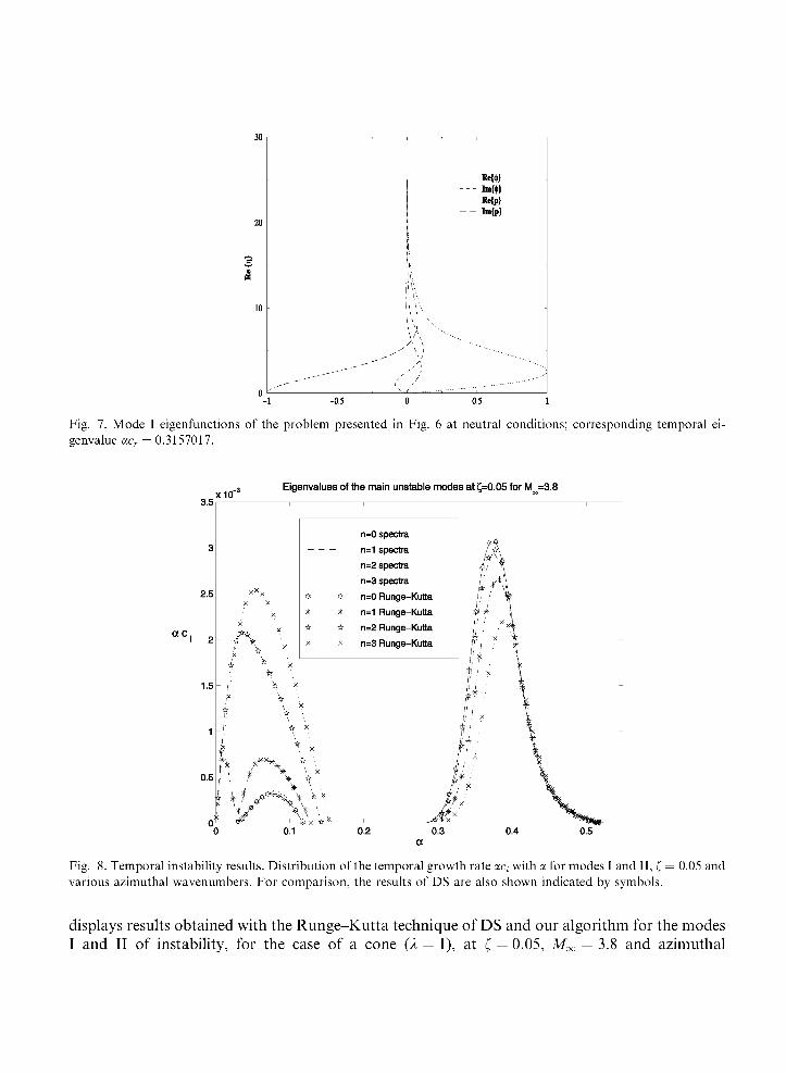
one Reviewer, the quality of the complex grid utilised, including resolution of the metric, can be assessed by presenting the eigenfunctions obtained by our algorithm; this result is shown in Fig. 7.

4.3.2. Supersonic flow on a cone The accuracy of the complex-grid spectral collocation algorithms presented in solving the linear

instability equations for supersonic flow past axisymmetric bodies is now assessed. The temporal linear instability analysis results of DS are used for comparisons with our predictions. Fig. 8

RetM Im{4>} Re{p} Im{p}

-0.5

\A / • \

\

/ 0 0.5

Fig. 7. Mode I eigenfunctions of the problem presented in Fig. 6 at neutral conditions; corresponding temporal ei-genvalue acr — 0.3157017.

Eigenvalues of the main unstable modes at £=0.05 for M =3.8

n=0 spectral

n=1 spectral

n=2 spectral

n=3 spectral

n=0 Runge-Kutta

n=1 Runge-Kutta

n=2 Runge-Kutta

n=3 Runge-Kutta

0.2

Fig. 8. Temporal instability results. Distribution of the temporal growth rate ac, with a for modes I and II, ( — 0.05 and various azimuthal wavenumbers. For comparison, the results of DS are also shown indicated by symbols.

displays results obtained with the Runge-Kutta technique of DS and our algorithm for the modes I and II of instability, for the case of a cone (1 = 1), at t, = 0.05, M^ = 3.8 and azimuthal

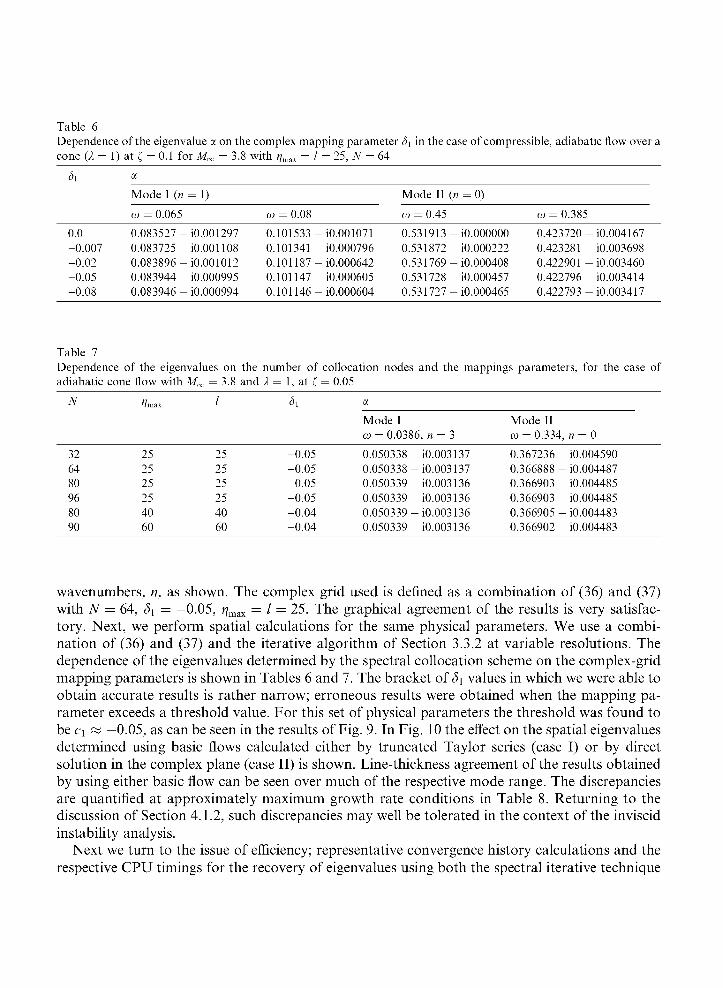
Table 6 Dependence of the eigenvalue a on the complex mapping parameter ¿i in the case of compressible, adiabatic flow over a cone (1 = 1) at C = 0.1 for M^ = 3.8 with f?max = / = 25, JV = 64

¿1

0.0 -0.007 -0.02 -0.05 -0.08

a

Mode I (n

w = 0.065

0.083527 -0.083725 -0.083896 -0.083944 -0.083946 -

= 1)

iO.001297 iO.001108 iO.001012 iO.000995 iO.000994

w = 0.08

0.101533-0.101341 -0.101187-0.101147-0.101146-

-iO.001071 - iO.000796 - iO.000642 - iO.000605 - iO.000604

Mode II (n = 0)

w = 0.45

0.531913-0.531872-0.531769-0.531728 -0.531727-

- iO.000000 - iO.000222 - iO.000408 - iO.000457 - iO.000465

w = 0.385

0.423720 -0.423281 -0.422901 -0.422796 -0.422793 -

-iO.004167 - iO.003698 - iO.003460 - iO.003414 - iO.003417

Table 7 Dependence of the eigenvalues on the number of collocation nodes and the mappings parameters, for the case of adiabatic cone flow with M^ — 3.8 and l — 1, at ( — 0.05

N

32 64 80 96 80 90

*7max

25 25 25 25 40 60

/

25 25 25 25 40 60

¿i

-0.05 -0.05 -0.05 -0.05 -0.04 -0.04

a

Mode I w = 0.0386, n = 3

0.050338-iO.003137 0.050338-iO.003137 0.050339-iO.003136 0.050339-iO.003136 0.050339-iO.003136 0.050339-iO.003136

Mode II m = 0.334, n = 0

0.367236 - iO.004590 0.366888 - iO.004487 0.366903 - iO.004485 0.366903 - iO.004485 0.366905 - iO.004483 0.366902 - iO.004483

wavenumbers, n, as shown. The complex grid used is defined as a combination of (36) and (37) with N = 64, Si = —0.05, r¡max = 1 = 25. The graphical agreement of the results is very satisfac-tory. Next, we perform spatial calculations for the same physical parameters. We use a combi­nation of (36) and (37) and the iterative algorithm of Section 3.3.2 at variable resolutions. The dependence of the eigenvalues determined by the spectral collocation scheme on the complex-grid mapping parameters is shown in Tables 6 and 7. The bracket of ¿i valúes in which we were able to obtain accurate results is rather narrow; erroneous results were obtained when the mapping pa­rameter exceeds a threshold valué. For this set of physical parameters the threshold was found to be c\ « —0.05, as can be seen in the results of Fig. 9. In Fig. 10 the effect on the spatial eigenvalues determined using basic flows calculated either by truncated Taylor series (case I) or by direct solution in the complex plañe (case II) is shown. Line-thickness agreement of the results obtained by using either basic flow can be seen over much of the respective mode range. The discrepancies are quantified at approximately máximum growth rate conditions in Table 8. Returning to the discussion of Section 4.1.2, such discrepancies may well be tolerated in the context of the inviscid instability analysis.

Next we turn to the issue of efficiency; representative convergence history calculations and the respective CPU timings for the recovery of eigenvalues using both the spectral iterative technique

Mode I, £=0.05, n=3, M =3.8,1=1

6, = -0.05

5, = -0.01

Mode II, £=0.05, n=0, M =3.8,1=1

Fig. 9. Effect of the mapping parameter valué on the accuracy of growth rate calculations for mode I nonaxisymmetric (n — 3) instabilities (upper) and mode II axisymmetric (n — 0) instabilities (lower), at ( — 0.05.

and the QZ algorithm are displayed in Table 9. The complex grid is defined as a combination of (36) and (37) with ¿h = —0.05, r¡max = / = 25 and the basic flow is calculated directly on the complex grid (case II). Results on two different platforms are presented here—a 100 MHz PC processor and a EV6 500 MHz Alpha processor. The timings presented were found to be

Mod© I, n=3, Mm=3.8,1=1, G=0.05 Mode I, n=3, M M = 3 . 8 , * = 1 , £=0.05

O 0.02 0.04 0.06 0.08 0.1 0.12 0.14 O 0.02 0.04 0.06 0.06 0.1 0.12 0.14

a m

Mode II, n=0,1^=3.8, X=1, ;=0.05 Mode II, n=0, M_=3.8, >=1, ;=0.05

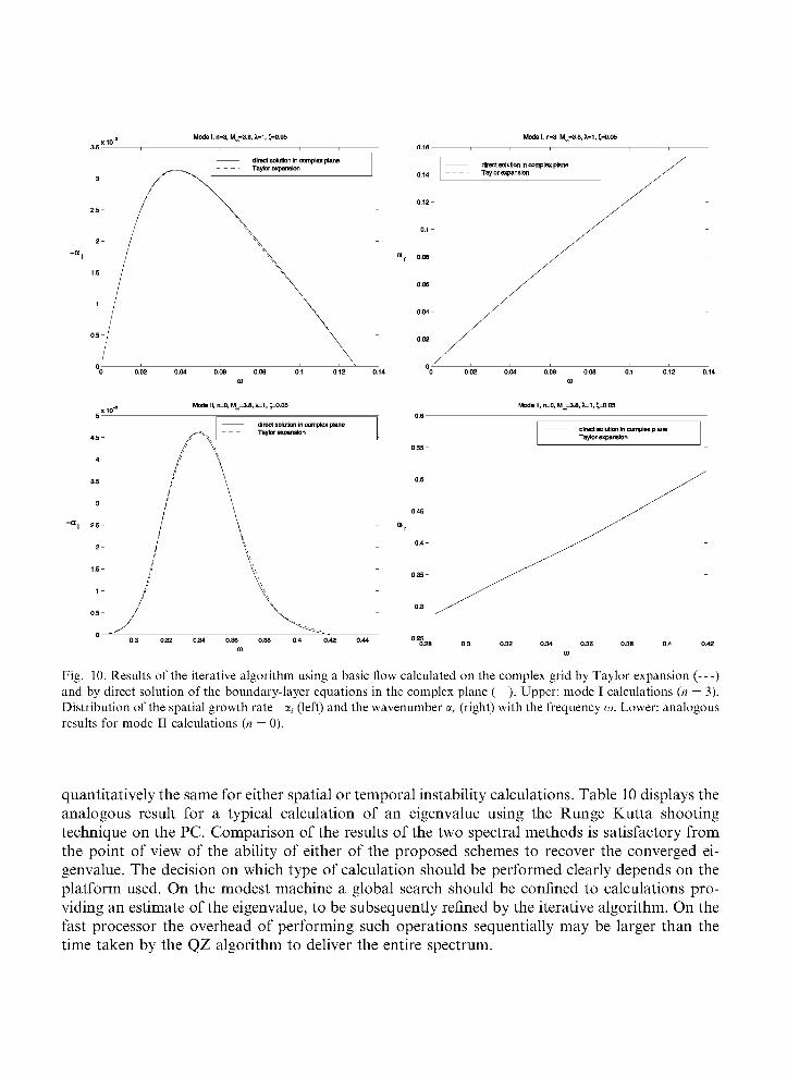
Fig. 10. Results of the iterative algorithm using a basic flow calculated on the complex grid by Taylor expansión (—) and by direct solution of the boundary-layer equations in the complex plañe (—). Upper: mode I calculations (n — 3). Distribution of the spatial growth rate -a, (left) and the wavenumber ar (right) with the frequency a>. Lower: analogous results for mode II calculations (n — 0).

quantitatively the same for either spatial or temporal instability calculations. Table 10 displays the analogous result for a typical calculation of an eigenvalue using the Runge-Kutta shooting technique on the PC. Comparison of the results of the two spectral methods is satisfactory from the point of view of the ability of either of the proposed schemes to recover the converged ei­genvalue. The decisión on which type of calculation should be performed clearly depends on the platform used. On the modest machine a global search should be confined to calculations pro-viding an estímate of the eigenvalue, to be subsequently refined by the iterative algorithm. On the fast processor the overhead of performing such operations sequentially may be larger than the time taken by the QZ algorithm to deliver the entire spectrum.

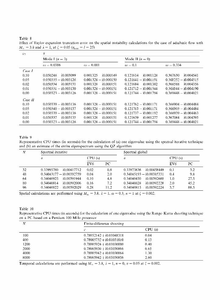
Table 8 Effect of Taylor expansión truncation error on the spatial instability calculations for the case of adiabatic flow with M^ = 3.8 and X = 1, at C = 0.05 (f?max = 1 = 25)

C2

Case I 0.10 0.05 0.02 0.01 0.00

Case II 0.10 0.05 0.02 0.01 0.00

a

Mode I (n = 3)

w = 0.0386

0.050248 -0.050335 -0.050334 -0.050331 -0.050323 -

0.050339 -0.050340 -0.050339 -0.050337 -0.050323 -

- iO.003099 -iO.003126 -iO.003131 -iO.003130 -iO.003126

-iO.003136 -iO.003137 -iO.003136 -iO.003135 -iO.003126

w = 0.001

0.001325-0.001328 -0.001328 -0.001328 -0.001328 -

0.001328 -0.001328 -0.001328 -0.001328 -0.001328 -

- iO.000149 -iO.000150 -iO.000151 -iO.000151 -iO.000151

-iO.000151 -iO.000151 -iO.000151 -iO.000151 -iO.000151

Mode II (Í

ra = 0.1

0.121614-0.121641 -0.121684-0.121712-0.121744-

0.121762-0.121763-0.121737-0.121639-0.121744-

i = 0)

-iO.001128 -iO.001191 -iO.001382 -iO.001544 -iO.001794

-iO.001171 -iO.001171 -iO.001192 - iO.001277 -iO.001794

w = 0.334

0.367630 -0.368252 -0.368588 -0.368844-0.369448 -

0.366904 -0.366903 -0.366939 -0.367084-0.369448 -

- iO.004541 -iO.004515 - iO.004356 - iO.004190 - iO.004021

- iO.004484 - iO.004484 - iO.004463 - iO.004395 - iO.004021

Table 9 Representative CPU times (in seconds) for the calculation of (a) one eigenvalue using the spectral iterative technique and (b) an estímate of the entire eigenspectrum using the QZ algorithm

N

32 48 64 80 96

Spectral iterative

a

0.33995780-iO.00417712 0.34043177 - iO.00392759 0.34040925 - iO.00391944 0.34040814 - iO.00392006 0.34040822 - iO.00392029

CPU (s)

EV6

0.02 0.04 0.10 0.16 0.28

PC

0.8 2.0 4.8 7.2

11.2

Spectral global

a

0.33973836 - iO.00458449 0.34045193-iO.00385331 0.34040450 - iO.00392688 0.34040828 - iO.00392228 0.34040815-iO.00392224

CPU (s)

EV6

0.1 0.4 1.0 2.0 3.7

PC

3.2 9.8

27.5 45.2 88.5

Spatial calculations are performed using M^ = 3.8, X = 1, co = 0.3, n = 1 at [ = 0.002.

Table 10 Representative CPU times (in seconds) for the calculation of one eigenvalue using the Runge-Kutta shooting technique on a PC based on a Pentium 100 MHz processor

N Finite-difference shooting

c CPU (s)

100 400 1200 2000 4000 8000

0.78052142-0.78005732-0.78005924-0.78005930-0.78005942-0.78005942-

iO.01048318 iO.01031010 iO.01030880 iO.01030866 iO.01030864 iO.01030856

0.04 0.13 0.40 0.65 1.30 2.60

Temporal calculations are performed using M^ = 3.8, X = 1, n = 0, a = 0.05 at ( = 0.002.

4.3.3. The effect offar-field boundary conditions As a final issue, we discuss the performance of the complex-grid algorithm in combination with

several different types of free-stream boundary conditions, typical of those used in inviscid linear instability analyses. We use the results of Fig. 10 as a reference and consider the combined effect of alternative boundary conditions with either the global or the local algorithm for the recovery of the eigenspectrum. Spatial instability is considered and three computational grids are used: (i) the first employs N = 64 collocation points and the domain is truncated at r¡max = 1 = 25; (ii) in the second grid the domain is truncated at r¡max = / = 60, while the number of collocation points is kept the same as in grid (i); (iii) and finally, resolution is increased in the third grid to N = 90 while

4

3

2.5

2

1.5

1

0.5

X10"3

"

/ ¡1

- / - i

-

/" /

1 f

Mode 1. C=005. n=3,

"" x

\ ^ V ..\

\ S'A

M_

\ V"-

\ v

\

=3.8,^=1

\

iterative. N=64

Q Z ' T1max=25, N = 6 4

QZ, ,nmax=601 N=64

QZ, Tl|Tlax=601 N=90

\

-

-

-

-

I, t=0.05, n=3, M =3.8,X=1

I I I

iterative, N=64

• QZ, n^^eo. N=90

i

y''

0 0.02 0.04 0.06 0.08 0.1 0.12 0.14 0.16 0.02 0.04 0.06 0.08 0.12 0.14

Mode II, C=0.05. n=0. MM=3.8,fc=1 Mode II, £=0.05, n=0, M H = 3 . 8 , X = 1

iterative, N=64

QZ.n m „=25 .N=64

QZ.-1„„=60,N=64

QZ, i l m =60, N=90

Iterative, N=64

QZ, ^,^^=25, N=64

QZ. Tlmln(=80, N=90

0.28 0.3 0.32 0.34 0.36 0.3B 0.4 0.42 0.3 0.32 0.34 0.36

Fig. 11. Results of the iterative algorithm employing the inhomogeneous boundary conditions (a) (—) and the global algorithm employing the homogeneous boundary conditions (b) (—, and • • •). Upper: mode I calculations (n — 3). Distribution of the spatial growth rate -a, (left) and the wavenumber ar (right) with the frequency a>. Lower: analogous results for mode II calculations (n — 0).

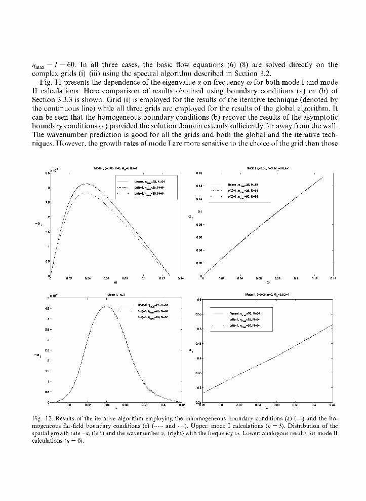
Vax = / = 60. In all three cases, the basic flow equations (6)-(8) are solved directly on the complex grids (i)-(iii) using the spectral algorithm described in Section 3.2.

Fig. 11 presents the dependence of the eigenvalue a on frequency co for both mode I and mode II calculations. Here comparison of results obtained using boundary conditions (a) or (b) of Section 3.3.3 is shown. Grid (i) is employed for the results of the iterative technique (denoted by the continuous line) while all three grids are employed for the results of the global algorithm. It can be seen that the homogeneous boundary conditions (b) recover the results of the asymptotic boundary conditions (a) provided the solution domain extends sufficiently far away from the wall. The wavenumber prediction is good for all the grids and both the global and the iterative tech-niques. However, the growth rates of mode I are more sensitive to the choice of the grid than those

Mode I, £=0.05, n=3, M_=3.8¿=1

0.161 i i i i

0.14 0 0.02 0.04 0.06 0.08 0.1 0.12 0.14 0)

Mods II, £=0.05, n=0, M_=3.8,l=1

0.61 i i i i

0.3 0.32 0.34 0.36 0.38 0.4 0.42 ' 0.28 0.3 0.32 0.34 0.36 0.36 0.4 0.42 G) <D

Fig. 12. Results of the iterative algorithm employing the inhomogeneous boundary conditions (a) (—) and the ho­mogeneous far-field boundary conditions (c) ( and • • •). Upper: mode I calculations (n — 3). Distribution of the spatial growth rate -a, (left) and the wavenumber ar (right) with the frequency a>. Lower: analogous results for mode II calculations (n — 0).

ModB I, £=0.05, n=3, Mn=3.8^=1

of mode II. Although the accuracy of the QZ results improves by taking ?7max further away from the cone surface, the number of collocation points considered is not sufficient for convergence. Increasing this to N = 90, accurate results for the growth rates of mode I instabilities can also be obtained. Fig. 12 again presents spatial results at the same parameter valúes, now obtained using the iterative algorithm alone and boundary conditions (a) or (c). An analogous conclusión may be drawn regarding the effect of truncating the domain too near the wall, with results being indis-tinguishable when the domain is truncated far from the solid surface. In other words, within the context of an iterative algorithm, necessarily used on account of the inhomogeneity of the boundary conditions, either type of boundary condition (a) or (c) may be used; the gains from truncating the domain near the wall and applying type (a) boundary conditions is marginal.

5. Discussion

Our concern in this paper has been with the generalised eigenvalue problem resulting from an inviscid linear instability analysis of wall-bounded boundary-layer type of flows. Such an analysis is motivated from a physical point of view by compressible laminar-turbulent flow transition prediction and from a numerical point of view by the need to tackle critical layers, the location of which cannot be predicted analytically, by appropriate numerical approaches. The numerical challenge of the resolution of critical layers has long been successfully met by robust finite-dif-ference/shooting algorithms [6,18]. The rather large number of discretisation nodes necessary for converged results to be obtained in both basic flow and eigenvalue problem calculations when using finite-diflerence/shooting algorithms is compensated by the sparse nature of the matrices involved; the resulting storage requirements can be handled straightforwardly by current hard­ware technology.

Here we have discussed alternative self-consistent algorithms based on complex-grid spectral methods for the numerical solution of the boundary-layer equations and the resulting inviscid linear eigenvalue problem, in a wide variety of flows of both academic and practical interest. We focused on examining the robustness of complex-grid calculations against variations of the grid parameters and presented both global and local algorithms for the calculation of the eigenvalues. Within either approach we posed the question of the effect of alternative forms of the boundary conditions on the accuracy of the instability results. Further, we examined the influence on the eigenvalue problem results of basic flow data generated either directly on complex collocation grids or using the corresponding real collocation points with the large gradients avoided by Taylor-expansion around the critical layer. Results were obtained for incompressible flow on planar geometries and compressible flow on both planar and axisymmetric curved geometries. In all cases studied, adequate resolution of the critical layer by the complex collocation grid spectral approach was found to deliver results in excellent agreement with established works. Further-more, we have identified the following directions for future research.

The most critical parameters on which instability results obtained on complex collocation grids were found to depend were those of the complex-grid mappings used. This is to be expected, since these parameters determine the means by which the critical layer is avoided and the re­sulting effective resolution used. Unfortunately, no general theory exists for the determination of the mapping parameters in the instability problem at hand and the optimal valúes can only be

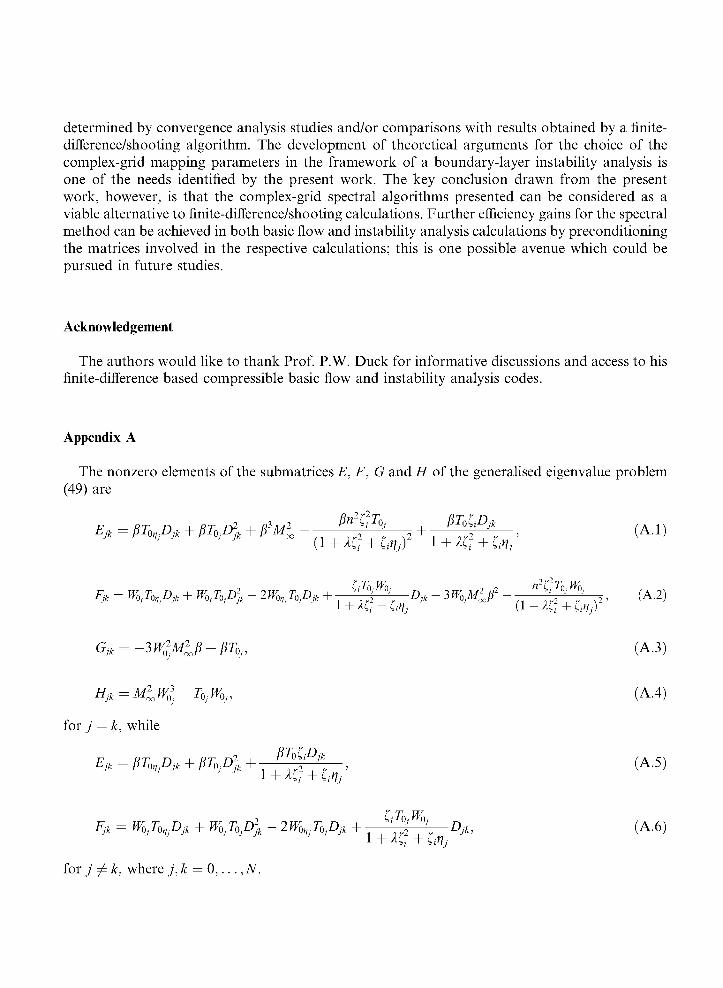
determined by convergence analysis studies and/or comparisons with results obtained by a finite-difference/shooting algorithm. The development of theoretical arguments for the choice of the complex-grid mapping parameters in the framework of a boundary-layer instability analysis is one of the needs identified by the present work. The key conclusión drawn from the present work, however, is that the complex-grid spectral algorithms presented can be considered as a viable alternative to finite-difference/shooting calculations. Further efficiency gains for the spectral method can be achieved in both basic flow and instability analysis calculations by preconditioning the matrices involved in the respective calculations; this is one possible avenue which could be pursued in future studies.

Acknowledgement

The authors would like to thank Prof. P.W. Duck for informative discussions and access to his finite-difference based compressible basic flow and instability analysis codes.

Appendix A

The nonzero elements of the submatrices E, F, G and H of the generalised eigenvalue problem (49) are

Fjk = W0¡T%Djk + W0]T0]D2

jk - 2W%T0jDjk + , , ° ' "' Djk + W^lf - " ]' °' °' 2, (A.2)

Gjk = -3W*M2ooP + pT0j, (A.3)

Hjk=MÍW03.-T0jW0j, (A.4)

for j = k, while

Ejk = PT%D]k + pT0jD% + f ^ f f k , (A.5)

C-Tr, Wi) Fjk = W,T%Djk + WoTopl - 2W%T,pjk + l> j Djk, (A.6)

l + K + Iñj

for j 7̂ k, where j , k = 0 , . . . , N.

Appendix B

The nonzero elements of the submatrices A\, A2, A?, and A4 of the system (51) are

Mjk = Djk + íi W0 %

1+1C-+C^ w^-p-

-iTn, 2jt

AH

A4jk

j = k, Ah*

A ,

yM2jw0j

i « 2 ( ^ -T0j

Djk

and

Djk

-P)

P) 1

2 r 2

1+- n2í « 2 ( 1 + 1 ^ + ^ - )

i(W0j-P)

for j 7̂ k, where j , k = 0 , 1 , . . . , N. The elements of vector b are given by bj = 0, if j¿N and j ¿ 2N,

bN=\[Kn+i(rii)+K\n-i\(rii)],

__Mliay{\-fi)Kn{ñi) U2N h 1 i n i

[\-Mi(\-P)2]1/2

where f/,. = ±a[l - i l £ ( l - /?)2]1/2(VC¿ +1C¿ + Vax),

and 7, k = 0,1 , . . . , N.

(B.l)

(B.2)

(B.3)

(B.4)

(B.5)

(B.6)

(B.7)

(B.8)

(B.9)

References

[1] Boyd JP. Complex coordínate methods for hydrodynamic instabilities and Sturm-Liouville eigenproblems with an interior singularity. J Comput Phys 1985;57(3):454-71.

[2] Boyd JP, Christidis ZD. Low wavenumber instability on the equatorial beta-plane. Geophys Res Lett 1982;9(7): 769-72.

[3] Bridges TJ, Morris PJ. Differential eigenvalue problems in which the parameter appears nonlinearly. J Comput Phys 1984;55(3):437-60.

[4] Canuto C, Hussaini MY, Quarteroni A, Zang TA. Spectral methods in fluid dynamics. Berlin: Springer; 1987. [5] Drazin PG, Reid WH. Hydrodynamic stability. Cambridge: Cambridge University Press; 1982. [6] Duck PW. The inviscid axisymmetric stability of the supersonic flow along a circular cylinder. J Fluid Mech

1990;214:611-37.

[7] Duck PW, Erlebacher G, Hussaini MY. On the linear stability of compressible plañe couette flow. J Fluid Mech 1994;258:131-65.

[8] Duck PW, Shaw SJ. The inviscid stability of supersonic flow past a sharp cone. Theoret Comput Fluid Dyn 1990;2:139-63.

[9] Fang Y, Reshotko E. Inviscid spatial stability of an axisymmetric compressible developing mixing layer. Technical Report TR EMAE/TR-97-217, Case Western Reserve Univ, Department of Mech and Aero Eng, 1997.

[10] Fang YC, Reshotko E. Inviscid spatial stability of a developing supersonic axisymmetric mixing layer. AIAA J 1999;37(l):23-8.

[11] Gilí AW, Sneddon GE. Complex mapped matrix methods in hydrodynamic stability problems. J Comput Phys 1995; 122(1): 13-24.

[12] Gilí AW, Sneddon GE. Pseudospectral methods and composite complex maps for near-boundary critical points. J Comput Phys 1996;129(l):l-7.

[13] Golub GH, van Loan CF. Matrix computations. 2nd ed. Baltimore: Johns Hopkins University Press; 1989. [14] Herbert Th. Parabolized stability equations. Ann Rev Fluid Mech 1997;29:245-83. [15] Hughes TH, Reid WH. On the stability of the asymptotic suction boundary layer profile. J Fluid Mech

1965;23:715-35. [16] Karabis A, Shaw SJ, Theofilis V. On the inviscid spatial instability of supersonic boundary layer flow along bodies

of revolution. In: Saric W, Fasel H, editors. Proceedings of the IUTAM Symposium on Laminar-Turbulent Transition, Sedona, AZ. 1999. p. 469-74.

[17] Macaraeg MG, Streett CL, Hussaini MY. A spectral collocation solution to the compressible stability eigenvalue problem. Technical Report TP 2858, NASA, 1988.

[18] Mack LM. Boundary layer stability theory. Technical Report 900-277, JPL, 1969. [19] Mack LM. Boundary layer linear stability theory. In AGARD Report No. 709, Special course on stability and

transition of laminar flow, p. 3-1-3-81, 1984. [20] Mack LM. Review of linear compressible stability theory. In: Dwoyer DL, Hussaini MY, editors. Stability of time

dependent and spatially varying flows ICASE Workshop on the Stability of Time Dependent and Spatially Varying Flows, New York. Berlin: Springer; 1987. p. 164-87.

[21] Mack LM. Stability of axisymmetric boundary layers on sharp cones at hypersonic Mach numbers. AIAA Paper 87-1413, 1987.

[22] Malik MR. Numerical methods for hypersonic boundary layer stability. J Comput Phys 1990;86(2):376^U3. [23] Mayer EW, Powell KG. Viscous and inviscid instabilities of a trailing vortex. J Fluid Mech 1992;245:91-114. [24] Otto SR, Denier JP. Numerical solution of a generalized elliptic partial differential eigenvalue problem. J Comput

Phys 1999;156(2):352-9. [25] Pruett CD, Streett CL. A spectral collocation method for compressible non-similar boundary layers. Int J Num

Meth Fluids 1991;13(6):713-37. [26] Reynolds O. An experimental investigation of the circumstances which determine whether the motion of water shall

be direct or sinuous and of the law of resistance in parallel channels. Phil Trans Roy Soc 1883;174:935-82. [27] Schubauer GB, Skramstad HK. Laminar boundary layer oscillations and stability of laminar flow. J Aero Sci

1947;14(2):69-78. [28] Shaw SJ, Duck PW. The inviscid stability of supersonic flow past heated or cooled axisymmetric bodies. Phys

Fluids 1992;4(7):1541-57. [29] Theofilis V. The discrete temporal eigenvalue spectrum of the generalized Hiemenz flow as solution of the Orr-

Sommerfeld equation. J Eng Math 1994;28(3):241-59. [30] Theofilis V. On linear and nonlinear instability of the incompressible swept attachment-line boundary layer. J Fluid

Mech 1998;355:193-227. [31] Theofilis V. On the resolution of critical flow regions in inviscid linear and nonlinear instability calculations. J Eng

Math 1998;34(l-2):lll-29. [32] Theofilis V. Advances in global linear instability theory. Prog Aero Sci (2002), in press. [33] Zaat JA. Numerische Beitráge zur Stabilitátstheorie der Grenzschichten. In: Grenzschichtforschung IUTAM

Symposium, Berlin. Berlin: Springer; 1958. p. 127-38.