Vector Autoregressive modeling of service delivery …eaas-journal.org/survey/userfiles/files/v6i302...

March. 2015. Vol. 6. No. 3 ISSN2305-8269

International Journal of Engineering and Applied Sciences © 2012 - 2015 EAAS & ARF. All rights reserved www.eaas-journal.org

11

VECTOR AUTOREGRESSIVE MODELING OF SERVICE

DELIVERY TOWARDS BOOSTING THE INTERNALLY

GENERATED REVENUE IN KWARA STATE, NIGERIA.

ABDULLAHI, GATTA ABDULGANIY, ADEWARA, ADEDAYO AMOS AND GATTA NUSIRAT

FUNMILAYO

Department of Statistics, University of Ilorin. Ilorin. Kwara State. Nigeria.

[email protected], [email protected] and [email protected]

ABSTRACT

Subjective method of forecasting has a great consequence on double taxation, rise in inflation rate

and uneven distribution of income, budget deficit etc. Therefore, it’s important to look into such situation

and provide the need to reduce the reliance of State Government on the Federal Allocation through

provision of reliable estimates of internally generated revenue so as to provide realistic budget

expenditures for the coming year and provides or sets standard performances for the system. The aim of

this research work is to forecast for the future demand in services of Permit, C of O, R of O, and Valuation

and consider how well one or more of these helps in predicting the other. Vector Autoregressive model has

been designed to examine the relationship that exist between set of variables and helps as well in

forecasting for the future occurrence of such events/variables. Based on the results of this research work, it

was found that C of O is the only variable that can be treated as endogenous variable given Permit and

Valuation and finally forecast was made which shows the highest and minimum values for the Permit, C of

O, R of O and Valuation with 960 & 54, 74 & 0, 86 & 0 and 41 & 0 at Jan 2017 and Oct 2015, April 2016

and Sept 2015, Oct 2016 and Dec 2013, Feb 2014 and Oct 2015 respectively, Government should use the

forecasts as a set target for each parastatal for revenue derive and eliminate redundancy in the workforce,

this will make the revenue projection more service deriving, reduced the inflation rate, eliminate double

taxation and budget deficit for a fixed service cost and propose efficient Recurrent Expenditure/Expenses.

Keywords: Certificate of Occupancy, Right of Occupancy, Permit, Valuation

INTRODUCTION

Vector auto-regression (VAR)

constitutes a special case of the more general

class of ARMA models. In essence, a VAR

model is a fairly unrestricted (flexible)

approximation to the reduced form of a wide

variety of dynamic econometric models. VAR

models can be specified in a number of ways.

Yt = c + Π1 Yt-1 + Π2 Yt-2 + ... + ΠpYt-p + t;

t = 1, ... , T, where Yt = {Y1t, Y2t, ... ,

Ynt), p is the lag length, Πi is an (n×n) matrix of

coefficients, t is the time period and n denotes

the numbers of endogenous variables.

According to Christopher (1980), VAR model is

a multivariate autoregressive model where each

variable is regressed on its past values and the

past values of the other variables in the system.

Model building in VAR models then depends on

the selection of the appropriate variables (based

on theory). The specification of the dynamic

structure proceeds based on testing for the

appropriate lag length using the sample data. He

argues that one of the critical contributions of the

VAR approach is that it can serve to define the

“battleground” of empirical debates about

multiple time series data. It does this by

providing a model of the dynamic and empirical

regularities of a set of related time series. VAR

would have p equations (in case we have p

variables), one for each variable. Each variable

would be regressed on its past values and the

past values of the other variable. The resulting

mailto:[email protected]



March. 2015. Vol. 6. No. 3 ISSN2305-8269


12

residuals (after checking for serial correlation)

would be exogenous shock or innovation. One

could look at the responses of each equation to

see how these “surprises” in each variable affect

the observed system. After accounting for these

dynamics, one could engage in inferences about

the Granger causal relationships between the

variables and try to determine the endogenous

structure and dynamics of the series.

He developed the approach of vector

autoregressive systems (VAR) as an alternative

to the traditional simultaneous equations system

approach. Starting from the autoregressive

representation of weakly stationary processes, all

included variables are assumed to be jointly

endogenous. Thus, in a VAR of order p

(VAR(p)), each component of the vector x

depends linearly on its own lagged values up to

p periods as well as on the lagged values of all

other variables up to order p. Therefore, our

starting point is the reduced form of the

econometric model. With such a model we can

find out whether a specific Granger causal

relation exists in the system. However, it has to

be mentioned that the number of variables that

can jointly be analyzed in such a system is quite

small; at least in the usual econometric

applications, this is limited by the number of

observations which are available. Nevertheless,

vector autoregressive systems play a crucial role

in modern approaches to analyze economic time

series.

The different equations of this system can be

estimated using Ordinary Least Square (OLS).

This leads to consistent estimates of the

parameters with the same efficiency as a

Generalized Least Squares Estimator. To

estimate the system, the order p i.e. the maximal

lag of the system, has to be determined. In order

to fix p, any of the following information criteria

can be used; the Final Prediction Error (FPE),

the Akaike Criterion (AIC), the Schwarz

Criterion (SC) and the Hannan-Quinn Criterion

(HQ).

The VAR methodology has been applied to a

vast range of empirical topic, including monetary

and fiscal policy analysis and short-term

economic forecasting. Also in the fields of

regional science and spatial economics the scope

of issue that could be addressed by means of

properly identified structural VARs appears to be

wide and includes: the analysis of the regional

propagation of demand shocks via trade

linkages; the assessment of long-run spatial

spillover effects from local public expenditure to

private sector performance; and the study of

dynamic knowledge externalities linking

patterning activity in the business sector to

academic research in nearby areas. However,

despite the fact that the VAR approach provides

a potentially useful analytical tool allowing for

the joint modeling of dynamic interdependencies

within a group of connected areas, until lately it

has received little attention in the applied spatial

economics literature.

In a multi-country set-up, cross-section

interactions were most recently dealt with by

Pesaran et al (2004), who introduced the Global

VAR specification, where information on trade

shares across countries is utilized to specify the

channels of transmission of national disturbances

across the world economy. Carlino and Defina

(1995) provide straightforward implementation

of the original Sims‟ approach, by fitting a VAR

model involving a single endogenous variable

(GNP) to the six regions in the US. In this case

the limited number of areas (6 regions) and short

lag order of the model allows the authors to

estimate an unrestricted reduced form VAR

specification. They are also among the first to

employ impulse response analysis based on VAR

estimation to measure the strength of spatial

spillover effects across regions. However, the

identification of structural shocks hinges on the

assumption of no contemporaneous spillover

effects, a hypothesis that can be overly restrictive

in many empirical settings.

Space-time impulse response analysis is also

dealt with by Giacinto (2006), who implements a

VAR approach based on an underlying

univariate STARMA (Space-Time ARMA)

specification. Prior information on spatial

contiguity is utilized both to place reasonable

restriction on VAR coefficients matrices and to

identify structural impulse responses. Lesage and

Pan (1995) introduced information on spatial

contiguity to specify the prior distribution of

VAR coefficients in a Bayesian univariate

regional VAR analysis. Canova and Ciccarelli

(2006) have recently proposed a multi-country

panel VAR specification that allows for cross-

sectional interdependence in a general

framework, in solving the incidental parameter

March. 2015. Vol. 6. No. 3 ISSN2305-8269


13

problem by imposing standard (i.e. non spatial)

prior distributional assumptions.

Christopher (1980) stated that; “if there is true

simultaneity among a set of variables, they

should all be treated on an equal footing; there

should not be any prior distinction between

endogenous and exogenous variables”.

Christopher (1972; 1980) pioneered the VAR

methodology, building on the idea of dynamic

decomposition of the variable in the system. He

rejected the use of standard simultaneous

equation models for three reasons:

*Identification restrictions on

parameters used in SEQ (simultaneous

equation) models are typically not based

on theory and thus may lead to incorrect

conclusions about the structure of the

models and the estimates.

*SEQ models are often based on

tenuous assumptions about the

exogeneity and endogeneity of the

variables. Because the true lag lengths

of the variables are not known a prior,

identification is then based on possibly

specious assumptions about exogeneity.

The formal identification of a dynamic

simultaneous equation model requires

that the exact true lag length to be

known for each variable; otherwise,

identification assumptions may not hold

(Hatanaka, 1975)

*If the variables in the model are

themselves policy projections,

additional identification problems will

be present because of temporal

restrictions. This is the rational

expectations critique: models are

typically treated as though ceteris

paribus claims will be true. In fact, they

are not, and then we need to be able to

assess the probabilistic implications of

different paths of the variables.

Meyler et al (1998) outlined autoregressive

integrated moving average (ARIMA) time series

models for forecasting inflation. They considered

two alternative approaches to the issue of

identifying ARIMA model-the Box Jenkins

approach and the objective penalty function

methods. The emphasis is on forecast

performance, which suggests that ARIMA

forecast has outperformed.

Parallel investigation which is done by Kenny et

al (1998) focused on the development of

multiple time series models for forecasting

inflation. The Bayesian approach to the

estimation of vector autoregressive (VAR) model

is employed. This allows the estimated models

combine the evidence in the data with any prior

information, which may also be available. A

large selection of inflation indicators is assessed

as potential candidates for inclusion in a VAR.

The results confirm the significant improvement

in forecasting performance, which can be

obtained by the use of Bayesian techniques.

Leheyda (2005) studied the determinants of

inflation in Ukraine through applying co-

integration analysis and error correction

modeling. A simple theoretical framework of

inflation for a small open economy is being

derived. The analysis is based upon three

hypotheses: excess money supply, foreign

inflation and cost-push inflation. Upon testing

for the existence of the long-run co-integration

relationships using Johansen procedure for the

sectoral VARs, a structural inflation function as

an equilibrium error correction model was

established. The long-run money demand,

purchasing power parity and mark-up

relationships where found, which may govern

prices in the long-run. In the short-run, inflation,

money supply, wages, exchange rate and real

output as well as some exogenous shocks

influence inflation dynamics.

Vizek and Broz (2007) analyze inflation in

Croatia in the period 1995-2006 using the co-

integration approach. They find out that mark-up

and excess money is the most significant

variables for explaining the short-run behaviour

of inflation. Furthermore, output gap, nominal

effective exchange rate, import prices, interest

rates and narrow money are also found to be

important in the influence on inflation.

Dejan (2007) made factor forecasts for the

overall inflation and the subcomponents (energy

inflation, industrial goods inflation, services

inflation, processed food and non-processed food

inflation) for Slovenia. The forecasts of the

factor model are compared to autoregressive

(AR) and vector autoregressive (VAR) models in

times of the Root mean squared error (RMSE).

In attrition, the factors were identified so as to

give interpretation to the forecasts. Results show

March. 2015. Vol. 6. No. 3 ISSN2305-8269


14

that the factor model is significantly better than

the AR benchmark forecasts and is not worse

from the VAR forecasts for all subcomponents

and the headline inflation, which render it a good

tool for forecasting inflation in Slovenia.

Christopher (1980), therefore, proposed method

for addressing the tenuous identification

problems of the SEQ approach is to focus on the

dynamic specification of the reduced form

model. This is in contrast to the SEQ approach,

which focuses on the identification choices in the

model specification. Sims‟ approach is to ensure

that the modelling approach to multiple time

series provides a complete characterization of the

dynamics of several series. This is done using a

multivariate autoregressive model to account for

the dynamics of all the variables. Building

multivariate time series models, according to the

VAR methodology, does not depend on a single

theory. Instead, a multiple theories can be

compared explicitly and evaluated (using

hypothesis testing) without the identification

assumptions that would be made in the

specification of alternative simultaneous

equation models. Because the variables in the

VAR model do not segment a prior into

endogenous and exogenous variables, we are less

likely to violate the model specification and

incorrectly induce simultaneity biases by

incorrectly specifying a variable as exogenous

when it is really endogenous.

Christopher (1980) opined that VAR modelers

also have a different conception of the interplay

of data and models. The goal of a VAR model is

to provide a probability model of the dynamics

and correlations among the data. Thus, VAR

models are considered best when based on a

simple, unbiased specification that accounts for

the uncertainty about the dynamics and the

model. To do this, pre-test biases must be

avoided (Pagan, 1978). Thus, unlike the

“specification-estimate-test-respecify” logic of

classical approaches, SEQ models, ARIMA

models, VAR models employ few hypothesis

tests to justify their specification. This leads to a

less biased representation of the model and its

dynamics rather than the false sense of precision

that can accompany other modeling strategies.

That is, once we have entered this cycle of

specification testing, the resulting inferences are

a function of the test procedure and are less

certain than the reported test statistics and

associated levels of significance or reported P

values would lead us to believe.

According to Simkins (1995), VAR models tend

to suffer from „over-fitting‟ with too many free

insignificant parameters. As a result, these

models can provide poor out-of-sample

forecasts, even though within-sample fitting is

good. Instead of restricting some of the

parameters in the usual way, Litterman (1986)

imposed a prior distribution on the parameters,

expressing the belief that many economic

variables behave like a random walk. Engle and

Granger (1987) concept of co-integration has

raised various interesting questions regarding the

forecasting ability of Error Correction Models

(ECM) over unrestricted VAR. Shoesmith (1992;

1995), Tegene and Kuchler (1994), and Wang

and Bessler (2004) provided empirical evidence

to suggest that ECM outperforms VAR in levels,

particularly over longer forecast horizons.

Shoesmith (1995) and Villani (2001), also

showed how Litterman‟s (1986) Bayes approach

can improve forecasting with co-integrated

VAR.

Stationary Vector Autoregressive Model

Let Yt= (y1t, y2t,...,ynt)T denote an (n )

vector of time series variables. The basic p lag

vector autoregressive (VAR (p)) model has the

form

Yt = c + Π1 Yt-1 + Π2 Yt-2 + ... + ΠpYt-p + t;

t = 1, ... , T, where c denotes an n 1

vector of constants and an n n matrix of

autoregressive coefficient for j=1,2,...,p. The

n 1 vector is a vector generalization of white

noise.

Unit Root Test

Before fitting a particular model to time series

data, the series must be made stationary.

Stationarity occurs in a time series when the

mean and autocovariances of the series remains

constant over the time series. Therefore, the

stochastic process is said to be stationary if

E ( ) = constant for all value of t

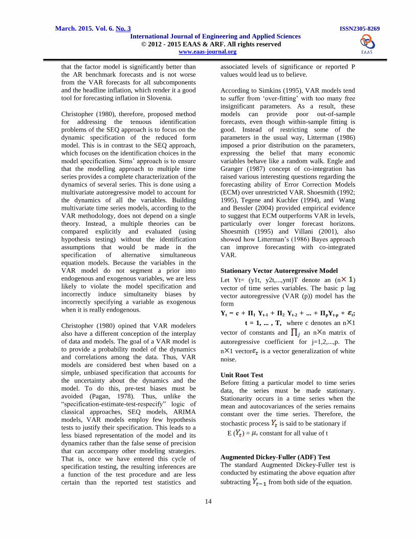
Augmented Dickey-Fuller (ADF) Test

The standard Augmented Dickey-Fuller test is

conducted by estimating the above equation after

subtracting from both side of the equation.

March. 2015. Vol. 6. No. 3 ISSN2305-8269


15

where and

Portmanteau Autocorrelation Test

The portmanteau test for residual autocorrelation

checks the null hypothesis that all residual

autocovariances are zero, that is,

Results from the data used

PERMIT C of O R of O VALUATION

Mean 372.1865 20.80163 24.01389 12.56699

Median 317.5661 20.80836 17.50000 12.70494

Maximum 2107 74 86 41

Minimum 58 0 0 0

Std. Dev. 314.1674 14.68590 18.64078 5.979959

Observations 72 72 72 72

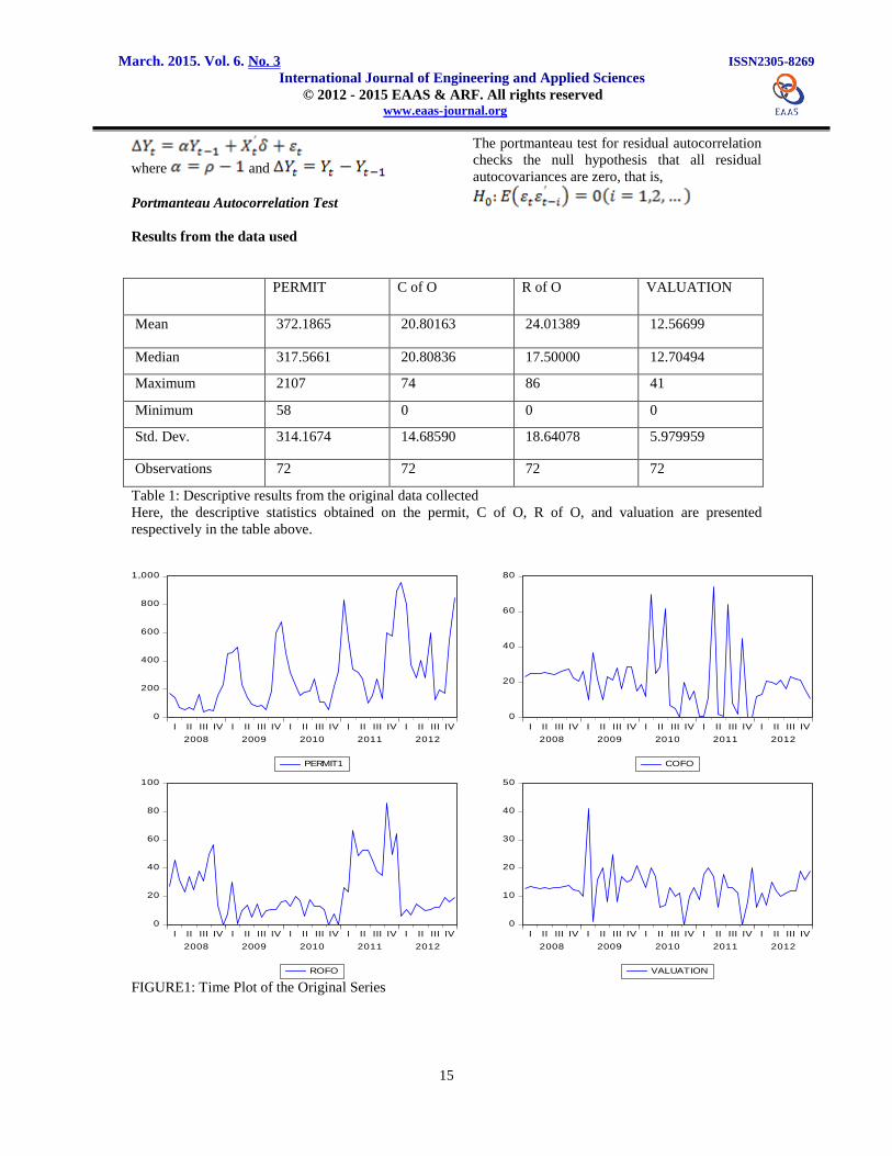
Table 1: Descriptive results from the original data collected

Here, the descriptive statistics obtained on the permit, C of O, R of O, and valuation are presented

respectively in the table above.

0

200

400

600

800

1,000

I II III IV I II III IV I II III IV I II III IV I II III IV

2008 2009 2010 2011 2012

PERMIT1

0

20

40

60

80


2008 2009 2010 2011 2012

COFO

0

20

40

60

80

100


2008 2009 2010 2011 2012

ROFO

0

10

20

30

40

50


2008 2009 2010 2011 2012

VALUATION FIGURE1: Time Plot of the Original Series

March. 2015. Vol. 6. No. 3 ISSN2305-8269


16

0

500

1,000

1,500

2,000

2,500

2008 2009 2010 2011 2012 2013

PERMIT

0

20

40

60

80

2008 2009 2010 2011 2012 2013

COFO

0

20

40

60

80

100

2008 2009 2010 2011 2012 2013

ROFO

0

10

20

30

40

50

2008 2009 2010 2011 2012 2013

VALUATION

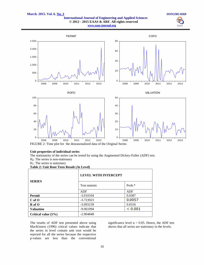
FIGURE 2: Time plot for the deseasonalized data of the Original Series

Unit properties of individual series

The stationarity of the series can be tested by using the Augmented Dickey-Fuller (ADF) test.

H0: The series is non-stationary

H1: The series is stationary

Table 2: Unit Root Tests Result (At Level)

SERIES

LEVEL WITH INTERCEPT

Test statistic Prob.*

ADF ADF

Permit -3.010104 0.0387

C of O -3.723923 R of O -3.093159 0.0316

Valuation -9.061094

Critical value (5%) -2.904848

The results of ADF test presented above using

MacKinnon (1996) critical values indicate that

the series in level contain unit root would be

rejected for all the series because the respective

p-values are less than the conventional

significance level α = 0.05. Hence, the ADF test

shows that all series are stationary in the levels.

March. 2015. Vol. 6. No. 3 ISSN2305-8269


17

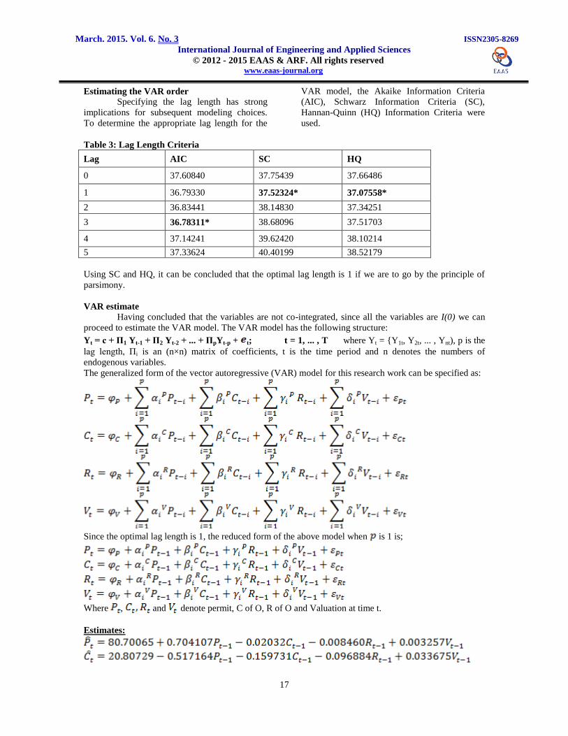
Estimating the VAR order

Specifying the lag length has strong

implications for subsequent modeling choices.

To determine the appropriate lag length for the

VAR model, the Akaike Information Criteria

(AIC), Schwarz Information Criteria (SC),

Hannan-Quinn (HQ) Information Criteria were

used.

Table 3: Lag Length Criteria

Lag AIC SC HQ

0 37.60840 37.75439 37.66486

1 36.79330 37.52324* 37.07558*

2 36.83441 38.14830 37.34251

3 36.78311* 38.68096 37.51703

4 37.14241 39.62420 38.10214

5 37.33624 40.40199 38.52179

Using SC and HQ, it can be concluded that the optimal lag length is 1 if we are to go by the principle of

parsimony.

VAR estimate

Having concluded that the variables are not co-integrated, since all the variables are I(0) we can

proceed to estimate the VAR model. The VAR model has the following structure:

Yt = c + Π1 Yt-1 + Π2 Yt-2 + ... + ΠpYt-p + t; t = 1, ... , T where Yt = {Y1t, Y2t, ... , Ynt), p is the

lag length, Πi is an (n×n) matrix of coefficients, t is the time period and n denotes the numbers of

endogenous variables.

The generalized form of the vector autoregressive (VAR) model for this research work can be specified as:

Since the optimal lag length is 1, the reduced form of the above model when is 1 is;

Where , and denote permit, C of O, R of O and Valuation at time t.

Estimates:

March. 2015. Vol. 6. No. 3 ISSN2305-8269


18

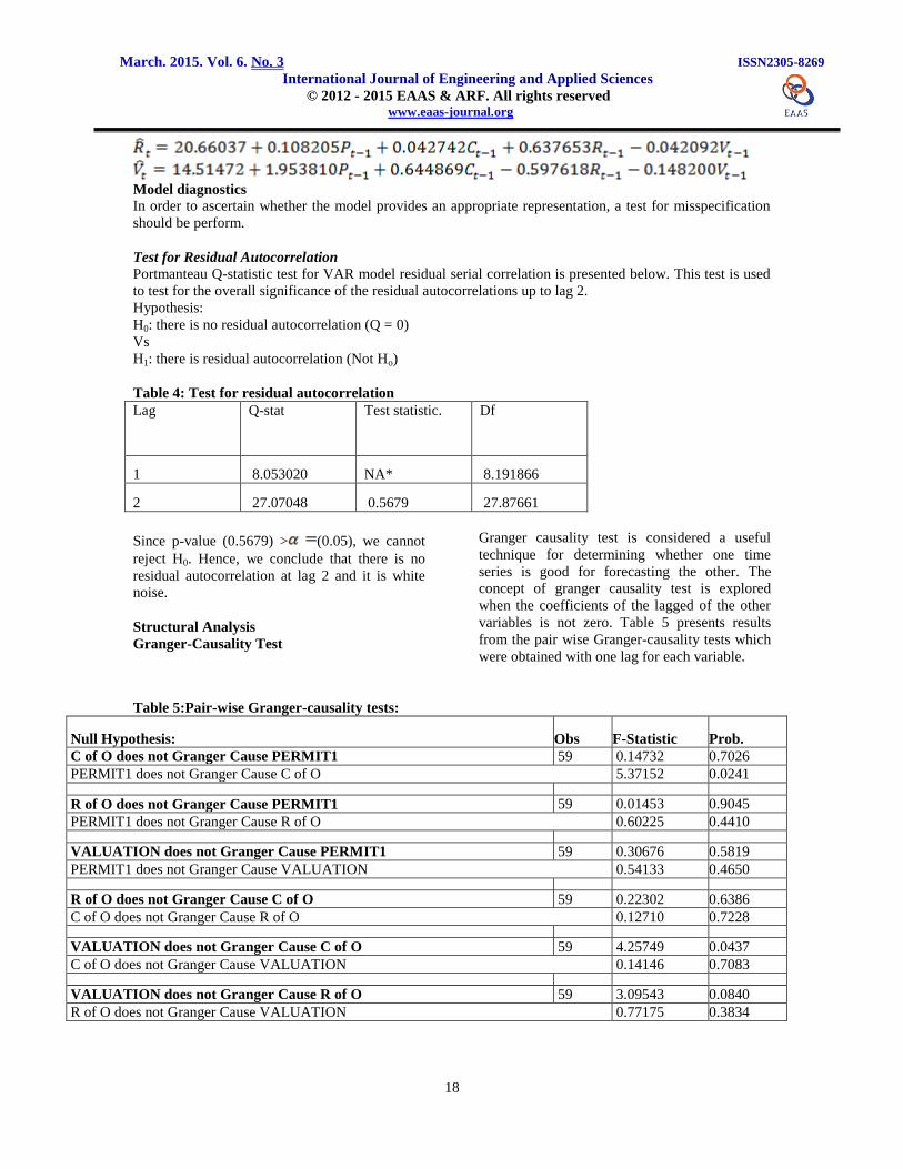
Model diagnostics

In order to ascertain whether the model provides an appropriate representation, a test for misspecification

should be perform.

Test for Residual Autocorrelation

Portmanteau Q-statistic test for VAR model residual serial correlation is presented below. This test is used

to test for the overall significance of the residual autocorrelations up to lag 2.

Hypothesis:

H0: there is no residual autocorrelation (Q = 0)

Vs

H1: there is residual autocorrelation (Not Ho)

Table 4: Test for residual autocorrelation

Lag Q-stat Test statistic. Df

1 8.053020 NA* 8.191866

2 27.07048 0.5679 27.87661

Since p-value (0.5679) > (0.05), we cannot

reject H0. Hence, we conclude that there is no

residual autocorrelation at lag 2 and it is white

noise.

Structural Analysis

Granger-Causality Test

Granger causality test is considered a useful

technique for determining whether one time

series is good for forecasting the other. The

concept of granger causality test is explored

when the coefficients of the lagged of the other

variables is not zero. Table 5 presents results

from the pair wise Granger-causality tests which

were obtained with one lag for each variable.

Table 5:Pair-wise Granger-causality tests:

Null Hypothesis: Obs F-Statistic Prob.

C of O does not Granger Cause PERMIT1 59 0.14732 0.7026

PERMIT1 does not Granger Cause C of O 5.37152 0.0241

R of O does not Granger Cause PERMIT1 59 0.01453 0.9045

PERMIT1 does not Granger Cause R of O 0.60225 0.4410

VALUATION does not Granger Cause PERMIT1 59 0.30676 0.5819

PERMIT1 does not Granger Cause VALUATION 0.54133 0.4650

R of O does not Granger Cause C of O 59 0.22302 0.6386

C of O does not Granger Cause R of O 0.12710 0.7228

VALUATION does not Granger Cause C of O 59 4.25749 0.0437

C of O does not Granger Cause VALUATION 0.14146 0.7083

VALUATION does not Granger Cause R of O 59 3.09543 0.0840

R of O does not Granger Cause VALUATION 0.77175 0.3834

March. 2015. Vol. 6. No. 3 ISSN2305-8269


19

The result shows that only Valuation granger cause C of O but the reverse is not true. This implies that the

relationship existing between valuation and C of O is unidirectional and that change in valuation

corresponds to change in C of O at 5% rejection level.

-.6

-.4

-.2

.0

.2

.4

.6

1 2 3 4 5 6 7 8 9 10 11 12

Cor(PERMIT1,PERMIT1(-i))

-.6

-.4

-.2

.0

.2

.4

.6

1 2 3 4 5 6 7 8 9 10 11 12

Cor(PERMIT1,COFO(-i))

-.6

-.4

-.2

.0

.2

.4

.6

1 2 3 4 5 6 7 8 9 10 11 12

Cor(PERMIT1,ROFO(-i))

-.6

-.4

-.2

.0

.2

.4

.6

1 2 3 4 5 6 7 8 9 10 11 12

Cor(PERMIT1,VALUATION(-i))

-.6

-.4

-.2

.0

.2

.4

.6

1 2 3 4 5 6 7 8 9 10 11 12

Cor(COFO,PERMIT1(-i))

-.6

-.4

-.2

.0

.2

.4

.6

1 2 3 4 5 6 7 8 9 10 11 12

Cor(COFO,COFO(-i))

-.6

-.4

-.2

.0

.2

.4

.6

1 2 3 4 5 6 7 8 9 10 11 12

Cor(COFO,ROFO(-i))

-.6

-.4

-.2

.0

.2

.4

.6

1 2 3 4 5 6 7 8 9 10 11 12

Cor(COFO,VALUATION(-i))

-.6

-.4

-.2

.0

.2

.4

.6

1 2 3 4 5 6 7 8 9 10 11 12

Cor(ROFO,PERMIT1(-i))

-.6

-.4

-.2

.0

.2

.4

.6

1 2 3 4 5 6 7 8 9 10 11 12

Cor(ROFO,COFO(-i))

-.6

-.4

-.2

.0

.2

.4

.6

1 2 3 4 5 6 7 8 9 10 11 12

Cor(ROFO,ROFO(-i))

-.6

-.4

-.2

.0

.2

.4

.6

1 2 3 4 5 6 7 8 9 10 11 12

Cor(ROFO,VALUATION(-i))

-.6

-.4

-.2

.0

.2

.4

.6

1 2 3 4 5 6 7 8 9 10 11 12

Cor(VALUATION,PERMIT1(-i))

-.6

-.4

-.2

.0

.2

.4

.6

1 2 3 4 5 6 7 8 9 10 11 12

Cor(VALUATION,COFO(-i))

-.6

-.4

-.2

.0

.2

.4

.6

1 2 3 4 5 6 7 8 9 10 11 12

Cor(VALUATION,ROFO(-i))

-.6

-.4

-.2

.0

.2

.4

.6

1 2 3 4 5 6 7 8 9 10 11 12

Cor(VALUATION,VALUATION(-i))

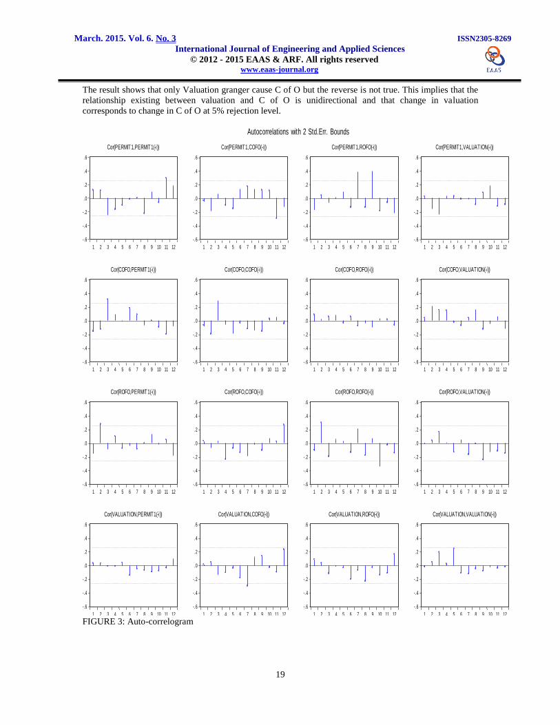
Autocorrelations with 2 Std.Err. Bounds

FIGURE 3: Auto-correlogram

March. 2015. Vol. 6. No. 3 ISSN2305-8269


20

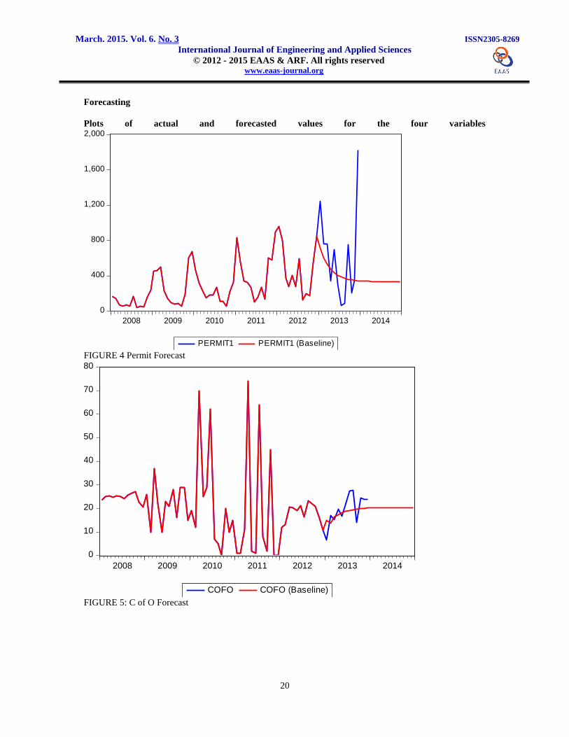
Forecasting

Plots of actual and forecasted values for the four variables

0

400

800

1,200

1,600

2,000

2008 2009 2010 2011 2012 2013 2014

PERMIT1 PERMIT1 (Baseline) FIGURE 4 Permit Forecast

0

10

20

30

40

50

60

70

80

2008 2009 2010 2011 2012 2013 2014

COFO COFO (Baseline)

FIGURE 5: C of O Forecast

March. 2015. Vol. 6. No. 3 ISSN2305-8269


21

0

10

20

30

40

50

60

70

80

90

2008 2009 2010 2011 2012 2013 2014

ROFO ROFO (Baseline)

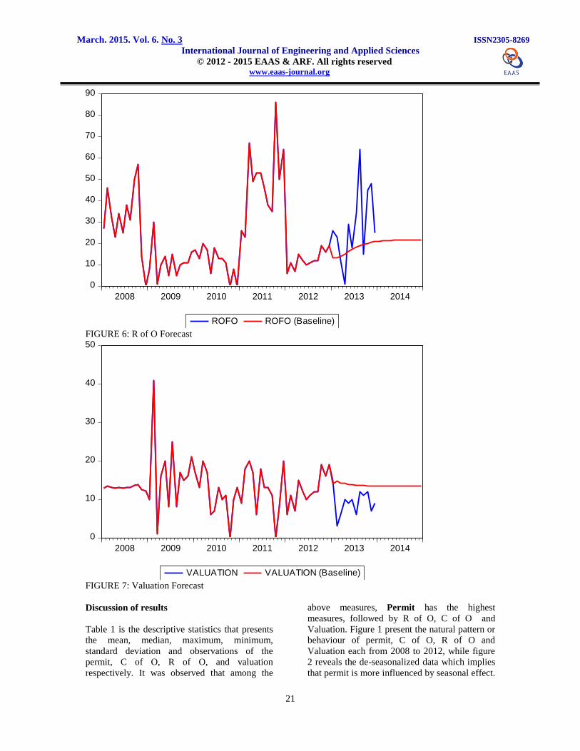
FIGURE 6: R of O Forecast

0

10

20

30

40

50

2008 2009 2010 2011 2012 2013 2014

VALUATION VALUATION (Baseline)

FIGURE 7: Valuation Forecast

Discussion of results

Table 1 is the descriptive statistics that presents

the mean, median, maximum, minimum,

standard deviation and observations of the

permit, C of O, R of O, and valuation

respectively. It was observed that among the

above measures, Permit has the highest

measures, followed by R of O, C of O and

Valuation. Figure 1 present the natural pattern or

behaviour of permit, C of O, R of O and

Valuation each from 2008 to 2012, while figure

2 reveals the de-seasonalized data which implies

that permit is more influenced by seasonal effect.

March. 2015. Vol. 6. No. 3 ISSN2305-8269


22

Table 2 is the unit root test result, which reveals

that the series is stationary at all level having

rejected the null hypothesis. In Table 3. the

optimum lag is obtained at lag 1, while Table 4

is the test for the presence of residual

autocorrelation in the model, Since p-value

(0.5679) > (0.05), we do not reject H0 and

conclude that there is no autocorrelation at lag 2

and it is white noise.

Table 5 shows that the model having passed the

unit root, the rejection of a null hypothesis

implies that one variable is granger caused by the

other, otherwise implies that one does not cause

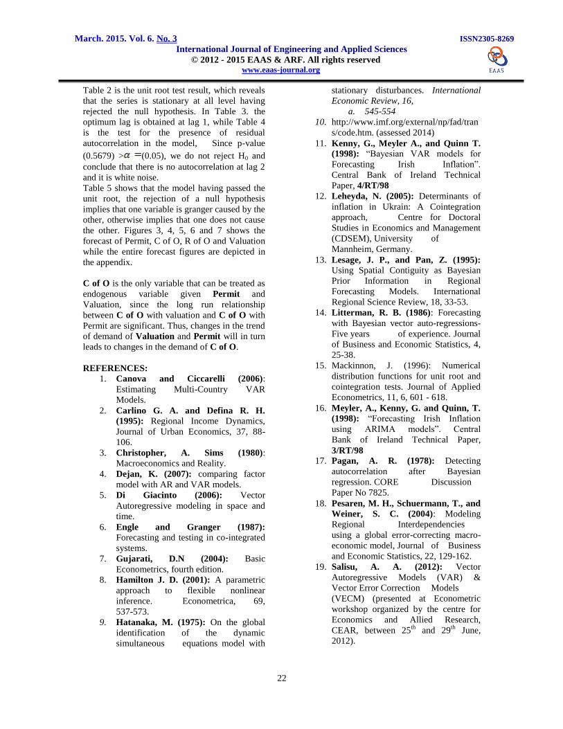
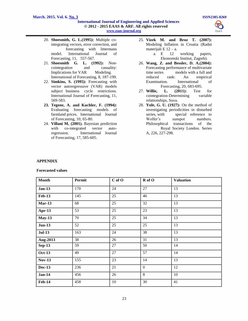
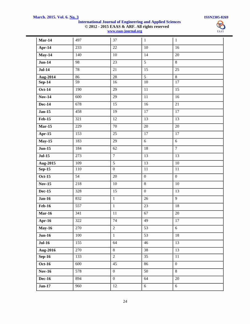
the other. Figures 3, 4, 5, 6 and 7 shows the

forecast of Permit, C of O, R of O and Valuation

while the entire forecast figures are depicted in

the appendix.

C of O is the only variable that can be treated as

endogenous variable given Permit and

Valuation, since the long run relationship

between C of O with valuation and C of O with

Permit are significant. Thus, changes in the trend

of demand of Valuation and Permit will in turn

leads to changes in the demand of C of O.

REFERENCES:

1. Canova and Ciccarelli (2006):

Estimating Multi-Country VAR

Models.

2. Carlino G. A. and Defina R. H.

(1995): Regional Income Dynamics,

Journal of Urban Economics, 37, 88-

106.

3. Christopher, A. Sims (1980):

Macroeconomics and Reality.

4. Dejan, K. (2007): comparing factor

model with AR and VAR models.

5. Di Giacinto (2006): Vector

Autoregressive modeling in space and

time.

6. Engle and Granger (1987): Forecasting and testing in co-integrated

systems.

7. Gujarati, D.N (2004): Basic

Econometrics, fourth edition.

8. Hamilton J. D. (2001): A parametric

approach to flexible nonlinear

inference. Econometrica, 69,

537-573.

9. Hatanaka, M. (1975): On the global

identification of the dynamic

simultaneous equations model with

stationary disturbances. International

Economic Review, 16,

a. 545-554

10. http://www.imf.org/external/np/fad/tran

s/code.htm. (assessed 2014)

11. Kenny, G., Meyler A., and Quinn T.

(1998): “Bayesian VAR models for

Forecasting Irish Inflation”.

Central Bank of Ireland Technical

Paper, 4/RT/98

12. Leheyda, N. (2005): Determinants of

inflation in Ukrain: A Cointegration

approach, Centre for Doctoral

Studies in Economics and Management

(CDSEM), University of

Mannheim, Germany.

13. Lesage, J. P., and Pan, Z. (1995):

Using Spatial Contiguity as Bayesian

Prior Information in Regional

Forecasting Models. International

Regional Science Review, 18, 33-53.

14. Litterman, R. B. (1986): Forecasting

with Bayesian vector auto-regressions-

Five years of experience. Journal

of Business and Economic Statistics, 4,

25-38.

15. Mackinnon, J. (1996): Numerical

distribution functions for unit root and

cointegration tests. Journal of Applied

Econometrics, 11, 6, 601 - 618.

16. Meyler, A., Kenny, G. and Quinn, T.

(1998): “Forecasting Irish Inflation

using ARIMA models”. Central

Bank of Ireland Technical Paper,

3/RT/98 17. Pagan, A. R. (1978): Detecting

autocorrelation after Bayesian

regression. CORE Discussion

Paper No 7825.

18. Pesaren, M. H., Schuermann, T., and

Weiner, S. C. (2004): Modeling

Regional Interdependencies

using a global error-correcting macro-

economic model, Journal of Business

and Economic Statistics, 22, 129-162.

19. Salisu, A. A. (2012): Vector

Autoregressive Models (VAR) &

Vector Error Correction Models

(VECM) (presented at Econometric

workshop organized by the centre for

Economics and Allied Research,

CEAR, between 25th

and 29th

June,

2012).

March. 2015. Vol. 6. No. 3 ISSN2305-8269


23

20. Shoesmith, G. L.(1995): Multiple co-

integrating vectors, error correction, and

forecasting with littermans

model. International Journal of

Forecasting, 11, 557-567.

21. Shoesmith G. L. (1992): Non-

cointegration and casuality:

Implications for VAR Modeling.

International of Forecasting, 8, 187-199.

22. Simkins, S. (1995): Forecasting with

vector autoregressuve (VAR) models

subject business cycle restrictions.

International Journal of Forecasting, 11,

569-583.

23. Tegene, A. and Kuchler, F. (1994): Evaluating forecasting models of

farmland prices. International Journal

of Forecasting, 10, 65-80.

24. Villani M, (2001). Bayesian prediction

with co-integrated vector auto-

regression. International Journal

of Forecasting, 17, 585-605.

25. Vizek M. and Broz T. (2007): Modeling Inflation in Croatia (Radni

materijali E 12 – a.

a. E 12 working papers,

Ekonomski Institut, Zagreb).

26. Wang, Z. and Bessler, D. A.(2004): Forecasting performance of multivariate

time series models with a full and

reduced rank: An empirical

Examination. International of

Forecasting, 20, 683-695.

27. Willie, L. (2011): Test for

cointegration-Determining variable

relationships, Suva.

28. Yule, G. U. (1927): On the method of

investigating periodicities in disturbed

series, with special reference to

Wolfer‟s sunspot numbers.

Philosophical transactions of the

Royal Society London. Series

A, 226, 227-298.

APPENDIX

Forecasted values

Month Permit C of O R of O Valuation

Jan-13 170 24 27 13

Feb-13 145 25 46 13

Mar-13 68 25 32 13

Apr-13 53 25 23 13

May-13 70 25 34 13

Jun-13 52 25 25 13

Jul-13 163 24 38 13

Aug-2013 38 26 31 13

Sep-13 59 27 50 14

Oct-13 49 27 57 14

Nov-13 155 23 14 13

Dec-13 236 21 0 12

Jan-14 456 26 8 10

Feb-14 458 10 30 41

March. 2015. Vol. 6. No. 3 ISSN2305-8269


24

Mar-14 497 37 1 1

Apr-14 233 22 10 16

May-14 140 10 14 20

Jun-14 98 23 5 8

Jul-14 78 21 15 25

Aug-2014 86 28 5 8

Sep-14 59 16 10 17

Oct-14 190 29 11 15

Nov-14 600 29 11 16

Dec-14 678 15 16 21

Jan-15 458 19 17 17

Feb-15 321 12 13 13

Mar-15 229 70 20 20

Apr-15 153 25 17 17

May-15 183 29 6 6

Jun-15 184 62 18 7

Jul-15 273 7 13 13

Aug-2015 109 5 13 10

Sep-15 110 0 11 11

Oct-15 54 20 0 0

Nov-15 218 10 8 10

Dec-15 328 15 0 13

Jan-16 832 1 26 9

Feb-16 557 1 23 18

Mar-16 341 11 67 20

Apr-16 322 74 49 17

May-16 270 2 53 6

Jun-16 100 1 53 18

Jul-16 155 64 46 13

Aug-2016 270 8 38 13

Sep-16 133 2 35 11

Oct-16 600 45 86 0

Nov-16 578 0 50 8

Dec-16 894 0 64 20

Jan-17 960 12 6 6

March. 2015. Vol. 6. No. 3 ISSN2305-8269


25

Feb-17 805 13 11 11

Mar-17 372 21 7 7

Apr-17 279 20 15 15

May-17 403 19 12 12

Jun-17 279 21 10 10

Jul-17 597 16 11 11

Aug-2017 125 23 12 12

Sep-17 199 22 12 12

Oct-17 174 21 19 19

Nov-17 548 16 16 16

Dec-17 847 11 19 19

Abbreviations and definitions used

IGR Internally Generated Revenue

C of O Certificate of Occupancy

R of O Right of Occupancy

PERMIT Approval For Development of Land

VALUATION Current Value as Land Appreciated

MICRO-ECONOMICS Between individual business and society

MACRO-ECONOMICS Between government business and a country

Vector Autoregressive modeling of service delivery …eaas-journal.org/survey/userfiles/files/v6i302...

Documents

Transcript of Vector Autoregressive modeling of service delivery …eaas-journal.org/survey/userfiles/files/v6i302...