Autoregressive Moving Average Models Under Exponential Power ...
Vector autoregressive Moving Average Process
Presented by
Muhammad Iqbal, Amjad Naveed
and Muhammad Nadeem
Road Map
1. Introduction
2. Properties of MA Finite Process
3. Stationarity of MA Process
4. VARMA (p,q) process
5. VAR (1) Representation of VARMA (p,q) Process
6. Autocovariance and Autocorrelation of VARMA (p,q) Process
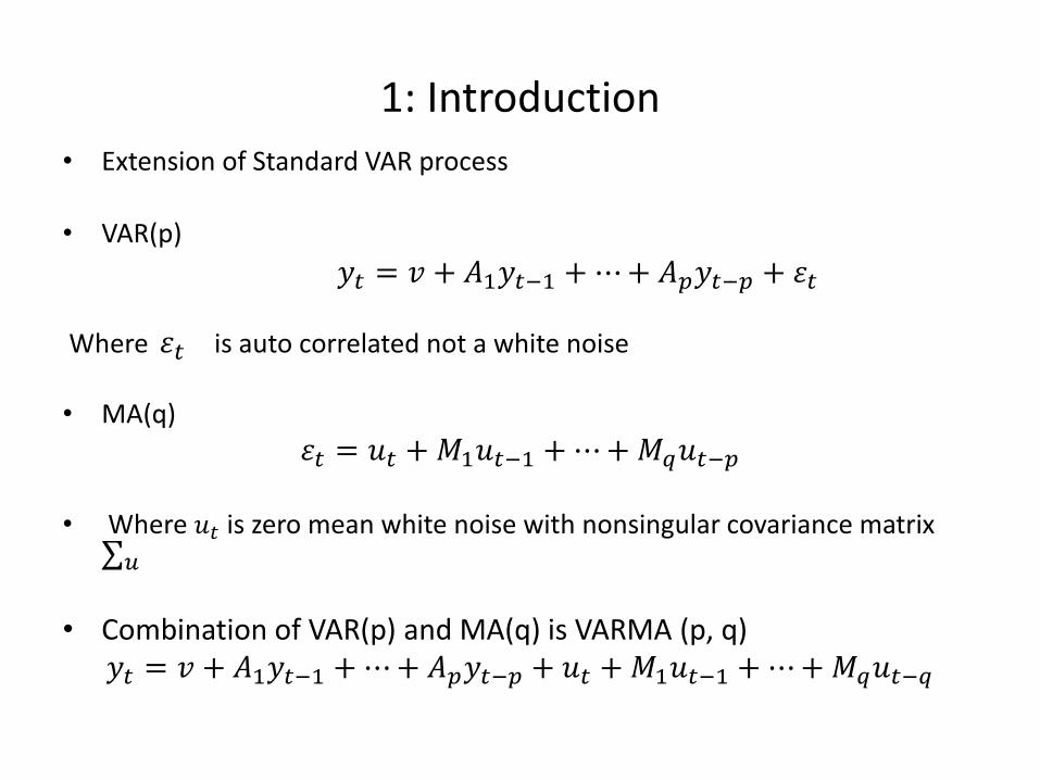
1: Introduction
• Extension of Standard VAR process
• VAR(p)
𝑦𝑡 = 𝑣 + 𝐴1𝑦𝑡−1 +⋯+ 𝐴𝑝𝑦𝑡−𝑝 + 𝜀𝑡
Where 𝜀𝑡 is auto correlated not a white noise • MA(q)
𝜀𝑡 = 𝑢𝑡 +𝑀1𝑢𝑡−1 +⋯+𝑀𝑞𝑢𝑡−𝑝 • Where 𝑢𝑡 is zero mean white noise with nonsingular covariance matrix
∑𝑢
• Combination of VAR(p) and MA(q) is VARMA (p, q) 𝑦𝑡 = 𝑣 + 𝐴1𝑦𝑡−1 +⋯+ 𝐴𝑝𝑦𝑡−𝑝 + 𝑢𝑡 +𝑀1𝑢𝑡−1 +⋯+𝑀𝑞𝑢𝑡−𝑞
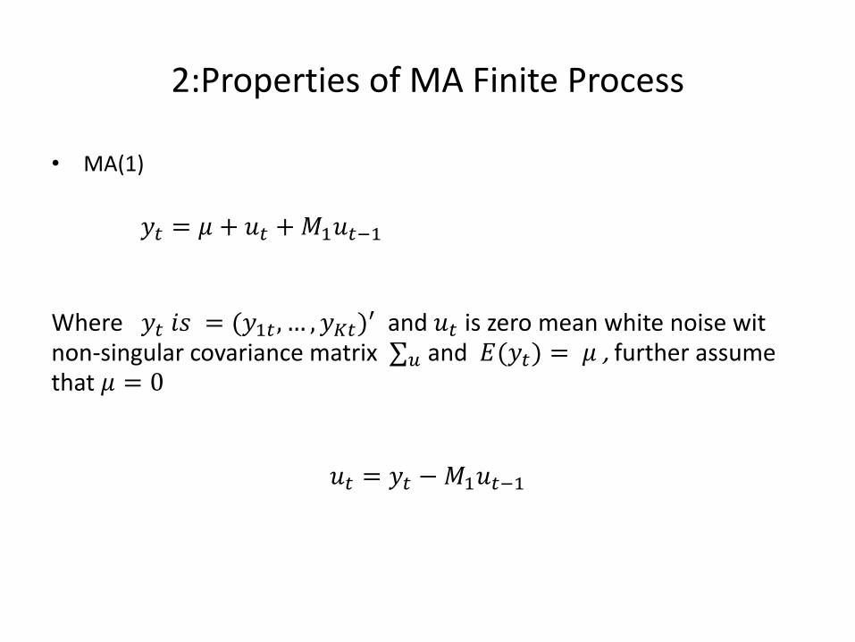
2:Properties of MA Finite Process
• MA(1)
𝑦𝑡 = 𝜇 + 𝑢𝑡 +𝑀1𝑢𝑡−1
Where 𝑦𝑡 𝑖𝑠 = (𝑦1𝑡 , … , 𝑦𝐾𝑡)′ and 𝑢𝑡 is zero mean white noise wit
non-singular covariance matrix ∑𝑢 and 𝐸(𝑦𝑡) = 𝜇 , further assume that 𝜇 = 0
𝑢𝑡 = 𝑦𝑡 −𝑀1𝑢𝑡−1
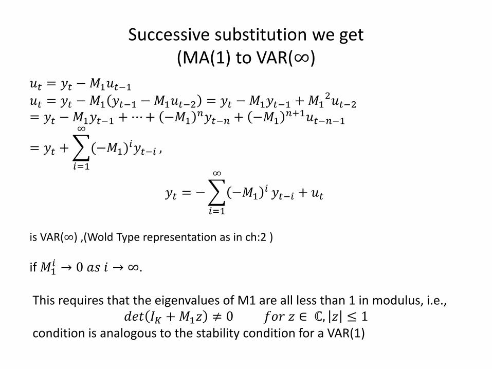
Successive substitution we get (MA(1) to VAR(∞)
𝑢𝑡 = 𝑦𝑡 −𝑀1𝑢𝑡−1
𝑢𝑡 = 𝑦𝑡 −𝑀1 𝑦𝑡−1 −𝑀1𝑢𝑡−2 = 𝑦𝑡 −𝑀1𝑦𝑡−1 +𝑀12𝑢𝑡−2
= 𝑦𝑡 −𝑀1𝑦𝑡−1 +⋯+ −𝑀1𝑛𝑦𝑡−𝑛 + −𝑀1
𝑛+1𝑢𝑡−𝑛−1
= 𝑦𝑡 + (−𝑀1)𝑖𝑦𝑡−𝑖
∞
𝑖=1
,
𝑦𝑡 = − −𝑀1𝑖
∞
𝑖=1
𝑦𝑡−𝑖 + 𝑢𝑡
is VAR(∞) ,(Wold Type representation as in ch:2 )
if 𝑀1𝑖 → 0 𝑎𝑠 𝑖 → ∞.
This requires that the eigenvalues of M1 are all less than 1 in modulus, i.e.,
𝑑𝑒𝑡 𝐼𝐾 +𝑀1𝑧 ≠ 0 𝑓𝑜𝑟 𝑧 ∈ ℂ, 𝑧 ≤ 1 condition is analogous to the stability condition for a VAR(1)
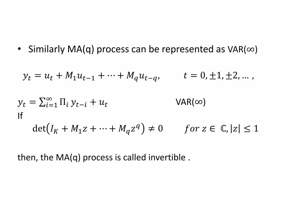
• Similarly MA(q) process can be represented as VAR(∞)
𝑦𝑡 = 𝑢𝑡 +𝑀1𝑢𝑡−1 +⋯+𝑀𝑞𝑢𝑡−𝑞 , 𝑡 = 0,±1,±2,… ,
𝑦𝑡 = ∑ Π𝑖∞𝑖=1 𝑦𝑡−𝑖 + 𝑢𝑡 VAR(∞)
If
det 𝐼𝐾 +𝑀1𝑧 + ⋯+𝑀𝑞𝑧𝑞 ≠ 0 𝑓𝑜𝑟 𝑧 ∈ ℂ, 𝑧 ≤ 1
then, the MA(q) process is called invertible .
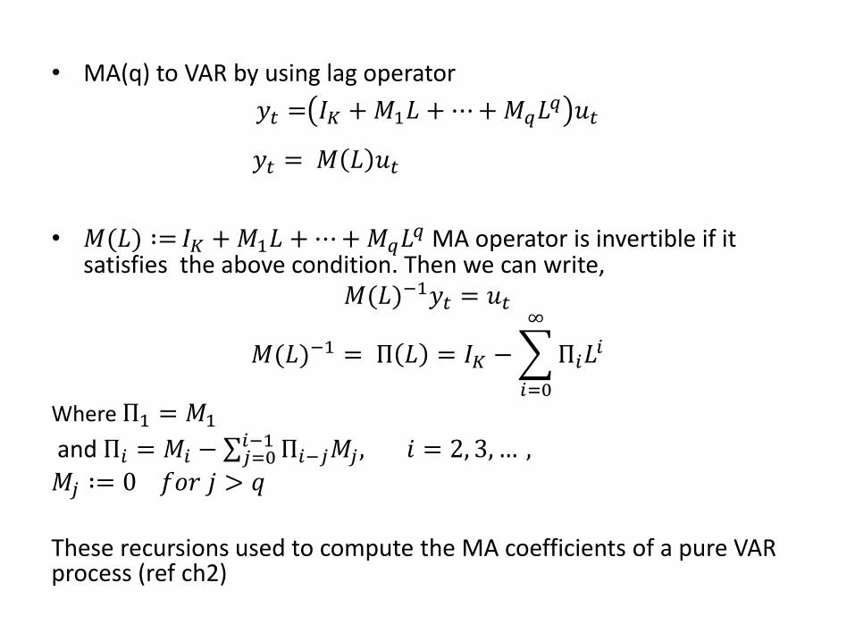
• MA(q) to VAR by using lag operator
𝑦𝑡 = 𝐼𝐾 +𝑀1𝐿 + ⋯+𝑀𝑞𝐿𝑞 𝑢𝑡
𝑦𝑡 = 𝑀 𝐿 𝑢𝑡
• 𝑀(𝐿) ∶= 𝐼𝐾 +𝑀1𝐿 +⋯+𝑀𝑞𝐿
𝑞 MA operator is invertible if it satisfies the above condition. Then we can write,
𝑀(𝐿)−1𝑦𝑡 = 𝑢𝑡
𝑀(𝐿)−1 = Π 𝐿 = 𝐼𝐾 − Π𝑖𝐿𝑖
∞
𝑖=0
Where Π1 = 𝑀1
and Π𝑖 = 𝑀𝑖 − ∑ Π𝑖−𝑗𝑀𝑗 , 𝑖 = 2, 3, … , 𝑖−1𝑗=0
𝑀𝑗 ∶= 0 𝑓𝑜𝑟 𝑗 > 𝑞
These recursions used to compute the MA coefficients of a pure VAR process (ref ch2)
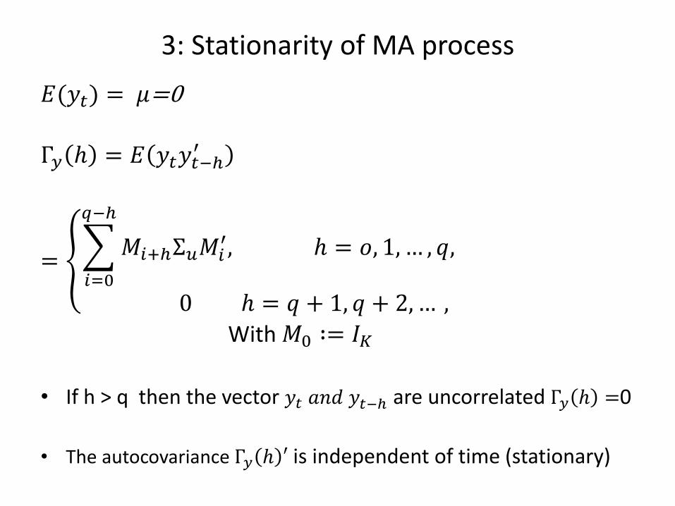
3: Stationarity of MA process 𝐸(𝑦𝑡) = 𝜇=0
Γ𝑦 ℎ = 𝐸 𝑦𝑡𝑦𝑡−ℎ
′
= 𝑀𝑖+ℎΣ𝑢𝑀𝑖
′, ℎ = 𝑜, 1, … , 𝑞,
𝑞−ℎ
𝑖=0
0 ℎ = 𝑞 + 1, 𝑞 + 2,… ,
With 𝑀0 ∶= 𝐼𝐾
• If h > q then the vector 𝑦𝑡 𝑎𝑛𝑑 𝑦𝑡−ℎ are uncorrelated Γ𝑦 ℎ =0
• The autocovariance Γ𝑦 ℎ ′ is independent of time (stationary)
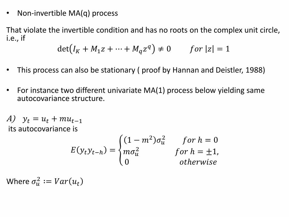
• Non-invertible MA(q) process
That violate the invertible condition and has no roots on the complex unit circle, i.e., if
det 𝐼𝐾 +𝑀1𝑧 + ⋯+𝑀𝑞𝑧𝑞 ≠ 0 𝑓𝑜𝑟 𝑧 = 1
• This process can also be stationary ( proof by Hannan and Deistler, 1988)
• For instance two different univariate MA(1) process below yielding same
autocovariance structure.
A) 𝑦𝑡 = 𝑢𝑡 +𝑚𝑢𝑡−1 its autocovariance is
𝐸 𝑦𝑡𝑦𝑡−ℎ = 1 −𝑚2 𝜎𝑢
2 𝑓𝑜𝑟 ℎ = 0
𝑚𝜎𝑢2 𝑓𝑜𝑟 ℎ = ±1,
0 𝑜𝑡ℎ𝑒𝑟𝑤𝑖𝑠𝑒
Where 𝜎𝑢
2 ∶= 𝑉𝑎𝑟 𝑢𝑡
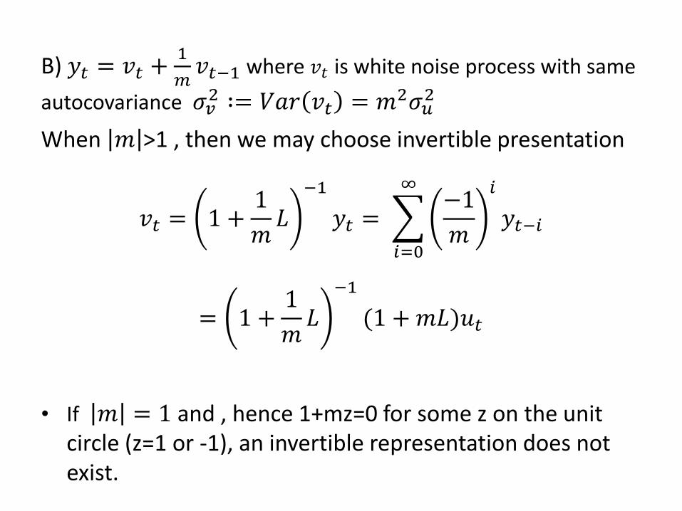
B) 𝑦𝑡 = 𝑣𝑡 +1
𝑚𝑣𝑡−1 where 𝑣𝑡 is white noise process with same
autocovariance 𝜎𝑣2 ∶= 𝑉𝑎𝑟 𝑣𝑡 = 𝑚2𝜎𝑢
2
When 𝑚 >1 , then we may choose invertible presentation
𝑣𝑡 = 1 +1
𝑚𝐿
−1
𝑦𝑡 = −1
𝑚
𝑖
𝑦𝑡−𝑖
∞
𝑖=0
= 1 +1
𝑚𝐿
−1
(1 +𝑚𝐿)𝑢𝑡
• If 𝑚 = 1 and , hence 1+mz=0 for some z on the unit circle (z=1 or -1), an invertible representation does not exist.
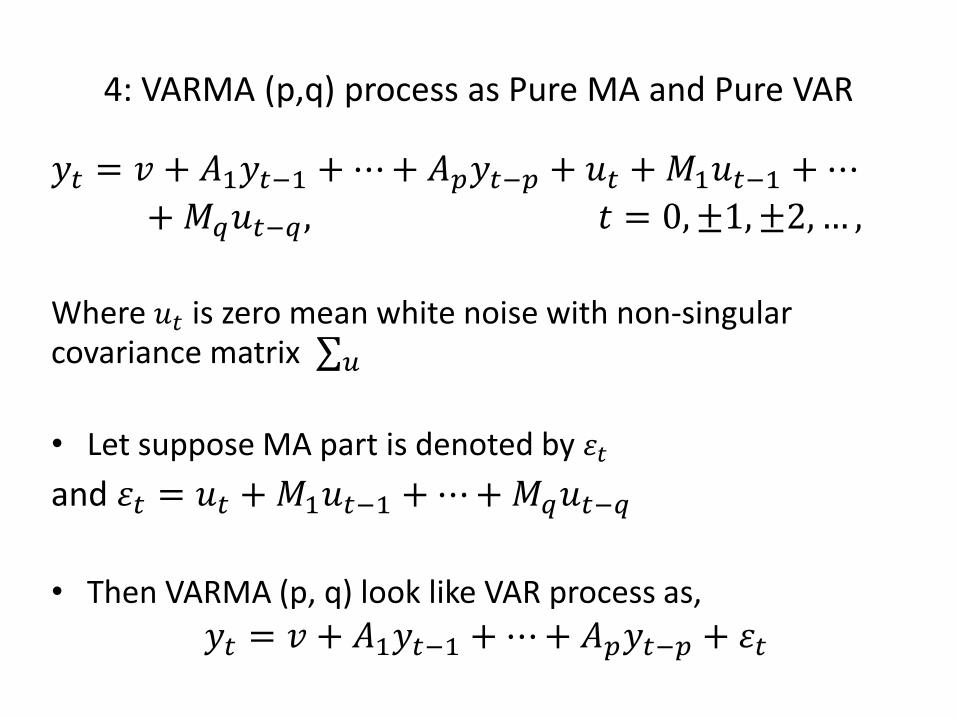
4: VARMA (p,q) process as Pure MA and Pure VAR
𝑦𝑡 = 𝑣 + 𝐴1𝑦𝑡−1 +⋯+ 𝐴𝑝𝑦𝑡−𝑝 + 𝑢𝑡 +𝑀1𝑢𝑡−1 +⋯
+𝑀𝑞𝑢𝑡−𝑞 , 𝑡 = 0,±1,±2,… ,
Where 𝑢𝑡 is zero mean white noise with non-singular covariance matrix ∑𝑢
• Let suppose MA part is denoted by 𝜀𝑡
and 𝜀𝑡 = 𝑢𝑡 +𝑀1𝑢𝑡−1 +⋯+𝑀𝑞𝑢𝑡−𝑞
• Then VARMA (p, q) look like VAR process as,
𝑦𝑡 = 𝑣 + 𝐴1𝑦𝑡−1 +⋯+ 𝐴𝑝𝑦𝑡−𝑝 + 𝜀𝑡
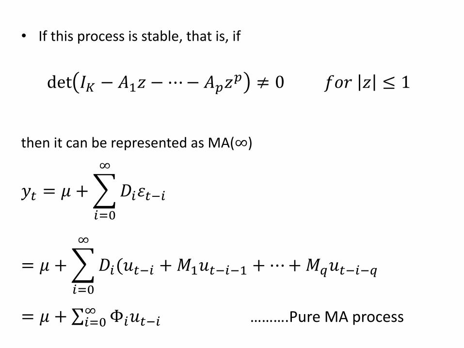
• If this process is stable, that is, if
det 𝐼𝐾 − 𝐴1𝑧 − ⋯− 𝐴𝑝𝑧𝑝 ≠ 0 𝑓𝑜𝑟 𝑧 ≤ 1
then it can be represented as MA(∞)
𝑦𝑡 = 𝜇 + 𝐷𝑖𝜀𝑡−𝑖
∞
𝑖=0
= 𝜇 + 𝐷𝑖(𝑢𝑡−𝑖
∞
𝑖=0
+𝑀1𝑢𝑡−𝑖−1 +⋯+𝑀𝑞𝑢𝑡−𝑖−𝑞
= 𝜇 + ∑ Φ𝑖𝑢𝑡−𝑖 ∞𝑖=0 ……….Pure MA process
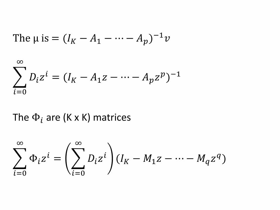
The μ is = (𝐼𝐾 − 𝐴1 −⋯− 𝐴𝑝)−1𝑣
𝐷𝑖𝑧𝑖
∞
𝑖=0
= (𝐼𝐾 − 𝐴1𝑧 − ⋯− 𝐴𝑝𝑧𝑝)−1
The Φ𝑖 are (K x K) matrices
Φ𝑖𝑧𝑖
∞
𝑖=0
= 𝐷𝑖𝑧𝑖
∞
𝑖=0
(𝐼𝐾 −𝑀1𝑧 −⋯−𝑀𝑞𝑧𝑞)
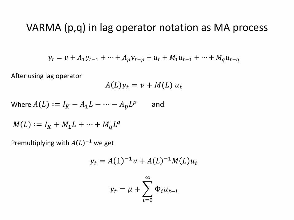
VARMA (p,q) in lag operator notation as MA process
𝑦𝑡 = 𝑣 + 𝐴1𝑦𝑡−1 +⋯+ 𝐴𝑝𝑦𝑡−𝑝 + 𝑢𝑡 +𝑀1𝑢𝑡−1 +⋯+𝑀𝑞𝑢𝑡−𝑞
After using lag operator
𝐴 𝐿 𝑦𝑡 = 𝑣 +𝑀(𝐿) 𝑢𝑡
Where 𝐴(𝐿) ∶= 𝐼𝐾 − 𝐴1𝐿 −⋯− 𝐴𝑝𝐿𝑝 and
𝑀 𝐿 ∶= 𝐼𝐾 +𝑀1𝐿 + ⋯+𝑀𝑞𝐿𝑞
Premultiplying with 𝐴 𝐿 −1 we get
𝑦𝑡 = 𝐴 1 −1𝑣 + 𝐴 𝐿 −1𝑀 𝐿 𝑢𝑡
𝑦𝑡 = 𝜇 + Φ𝑖𝑢𝑡−𝑖
∞
𝑖=0
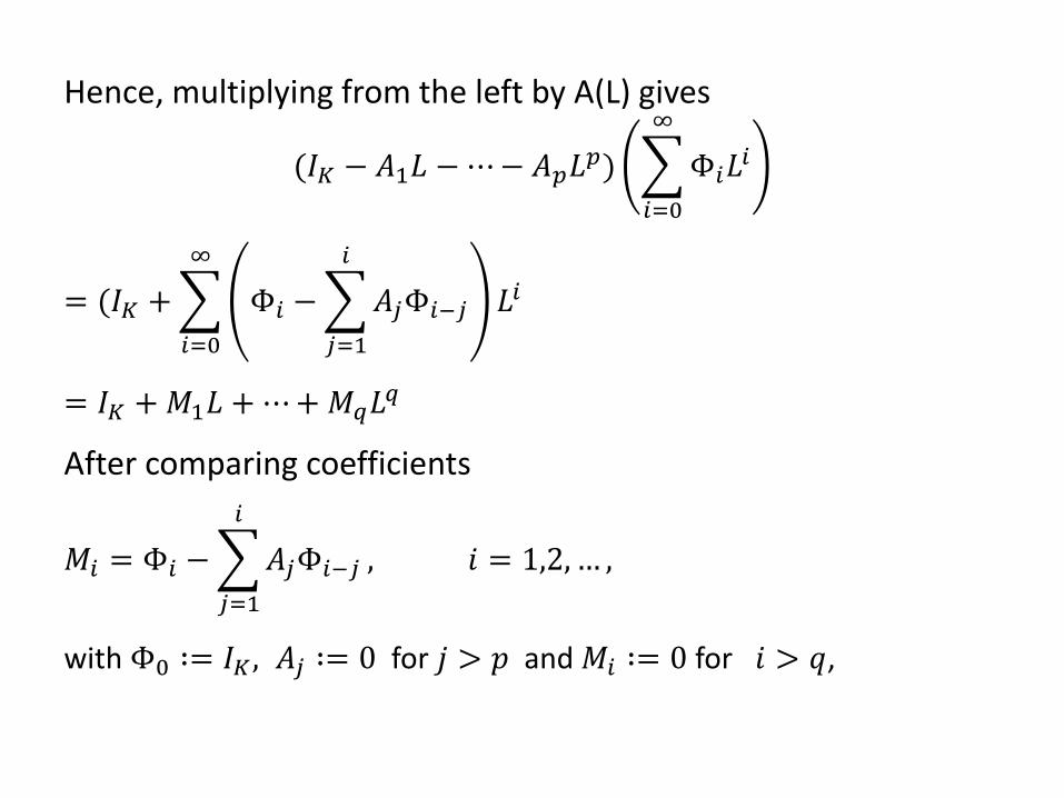
Hence, multiplying from the left by A(L) gives
(𝐼𝐾 − 𝐴1𝐿 −⋯− 𝐴𝑝𝐿𝑝) Φ𝑖𝐿
𝑖
∞
𝑖=0
= (𝐼𝐾 + Φ𝑖 − 𝐴𝑗Φ𝑖−𝑗
𝑖
𝑗=1
∞
𝑖=0
𝐿𝑖
= 𝐼𝐾 +𝑀1𝐿 + ⋯+𝑀𝑞𝐿𝑞
After comparing coefficients
𝑀𝑖 = Φ𝑖 − 𝐴𝑗Φ𝑖−𝑗
𝑖
𝑗=1
, 𝑖 = 1,2,… ,
with Φ0 ∶= 𝐼𝐾 , 𝐴𝑗 ∶= 0 for 𝑗 > 𝑝 and 𝑀𝑖 ∶= 0 for 𝑖 > 𝑞,
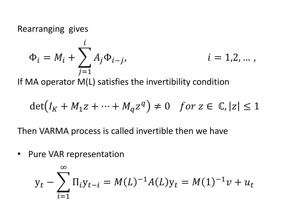
Rearranging gives
Φ𝑖 = 𝑀𝑖 + 𝐴𝑗Φ𝑖−𝑗 , 𝑖 = 1,2, … ,
𝑖
𝑗=1
If MA operator M(L) satisfies the invertibility condition
det 𝐼𝐾 +𝑀1𝑧 + ⋯+𝑀𝑞𝑧𝑞 ≠ 0 𝑓𝑜𝑟 𝑧 ∈ ℂ, 𝑧 ≤ 1
Then VARMA process is called invertible then we have • Pure VAR representation
y𝑡 − Π𝑖y𝑡−𝑖
∞
𝑖=1
= 𝑀 𝐿 −1𝐴 𝐿 y𝑡 = 𝑀 1 −1𝑣 + 𝑢𝑡
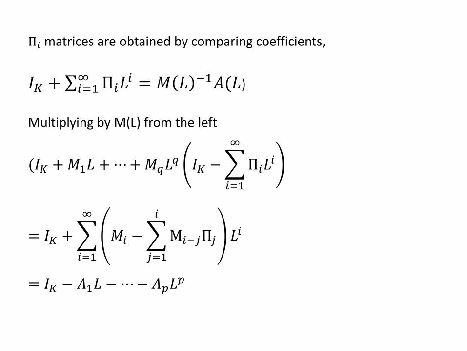
Π𝑖 matrices are obtained by comparing coefficients,
𝐼𝐾 + ∑ Π𝑖𝐿𝑖∞
𝑖=1 = 𝑀 𝐿 −1𝐴(𝐿)
Multiplying by M(L) from the left
(𝐼𝐾 +𝑀1𝐿 +⋯+𝑀𝑞𝐿𝑞 𝐼𝐾 − Π𝑖𝐿
𝑖
∞
𝑖=1
= 𝐼𝐾 + 𝑀𝑖 − M𝑖−𝑗Π𝑗
𝑖
𝑗=1
∞
𝑖=1
𝐿𝑖
= 𝐼𝐾 − 𝐴1𝐿 −⋯− 𝐴𝑝𝐿𝑝
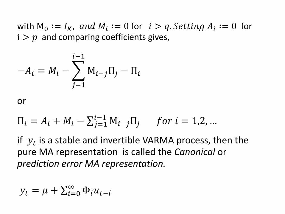
with M0 ∶= 𝐼𝐾 , 𝑎𝑛𝑑 𝑀𝑖 ∶= 0 for 𝑖 > 𝑞. 𝑆𝑒𝑡𝑡𝑖𝑛𝑔 𝐴𝑖 ∶= 0 for i > 𝑝 and comparing coefficients gives,
−𝐴𝑖 = 𝑀𝑖 − M𝑖−𝑗Π𝑗
𝑖−1
𝑗=1
− Π𝑖
or
Π𝑖 = 𝐴𝑖 +𝑀𝑖 −∑ M𝑖−𝑗Π𝑗 𝑓𝑜𝑟 𝑖 = 1,2, …𝑖−1𝑗=1
if 𝑦𝑡 is a stable and invertible VARMA process, then the pure MA representation is called the Canonical or prediction error MA representation.
𝑦𝑡 = 𝜇 + ∑ Φ𝑖𝑢𝑡−𝑖∞𝑖=0
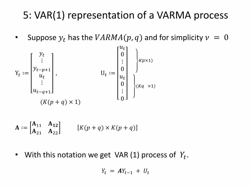
5: VAR(1) representation of a VARMA process
• Suppose 𝑦𝑡 has the 𝑉𝐴𝑅𝑀𝐴(𝑝, 𝑞) and for simplicity 𝜈 = 0
Y𝑡 ∶=
𝑦𝑡⋮
𝑦𝑡−𝑝+1𝑢𝑡⋮
𝑢𝑡−𝑞+1
, U𝑡 ∶=
𝑢𝑡0⋮0𝑢𝑡0⋮0
𝐾𝑝×1)
(𝐾𝑞 ×1)
(𝐾(𝑝 + 𝑞) × 1)
𝐀 ∶=𝐀11 𝐀𝟏𝟐
𝐀21 𝐀22 𝐾(𝑝 + 𝑞) × 𝐾(𝑝 + 𝑞)
• With this notation we get VAR (1) process of 𝑌𝑡.
𝑌𝑡 = 𝑨𝑌𝑡−1 + 𝑈𝑡
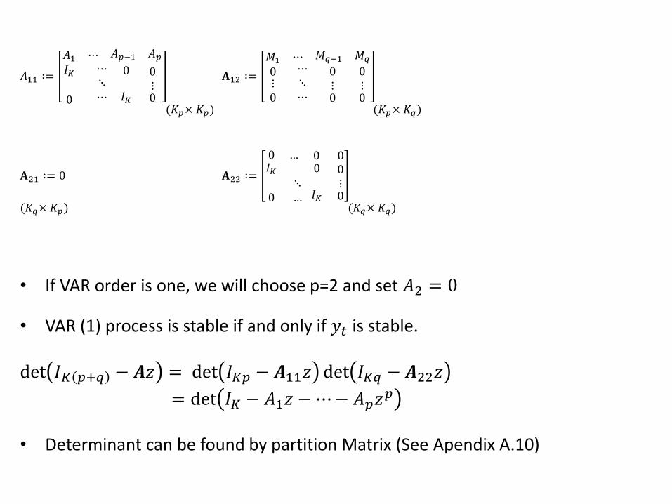
𝐴11 ∶=
𝐴1 ⋯ 𝐴𝑝−1 𝐴𝑝𝐼𝐾
0
⋯⋱⋯
0
𝐼𝐾 0⋮0
𝐀12 ∶=
𝑀1 ⋯ 𝑀𝑞−1 𝑀𝑞
0⋮0
⋯⋱⋯
0⋮0
0⋮0
(𝐾𝑝× 𝐾𝑝) (𝐾𝑝× 𝐾𝑞)
𝐀21 ∶= 0 𝐀22 ∶=
0 … 0 0𝐼𝐾
0
⋱…
0
𝐼𝐾 0⋮0
(𝐾𝑞× 𝐾𝑝) (𝐾𝑞× 𝐾𝑞)
• If VAR order is one, we will choose p=2 and set 𝐴2 = 0
• VAR (1) process is stable if and only if 𝑦𝑡 is stable.
det 𝐼𝐾 𝑝+𝑞 − 𝑨𝑧 = det 𝐼𝐾𝑝 − 𝑨11𝑧 det 𝐼𝐾𝑞 − 𝑨22𝑧
= det 𝐼𝐾 − 𝐴1𝑧 − ⋯− 𝐴𝑝𝑧𝑝
• Determinant can be found by partition Matrix (See Apendix A.10)
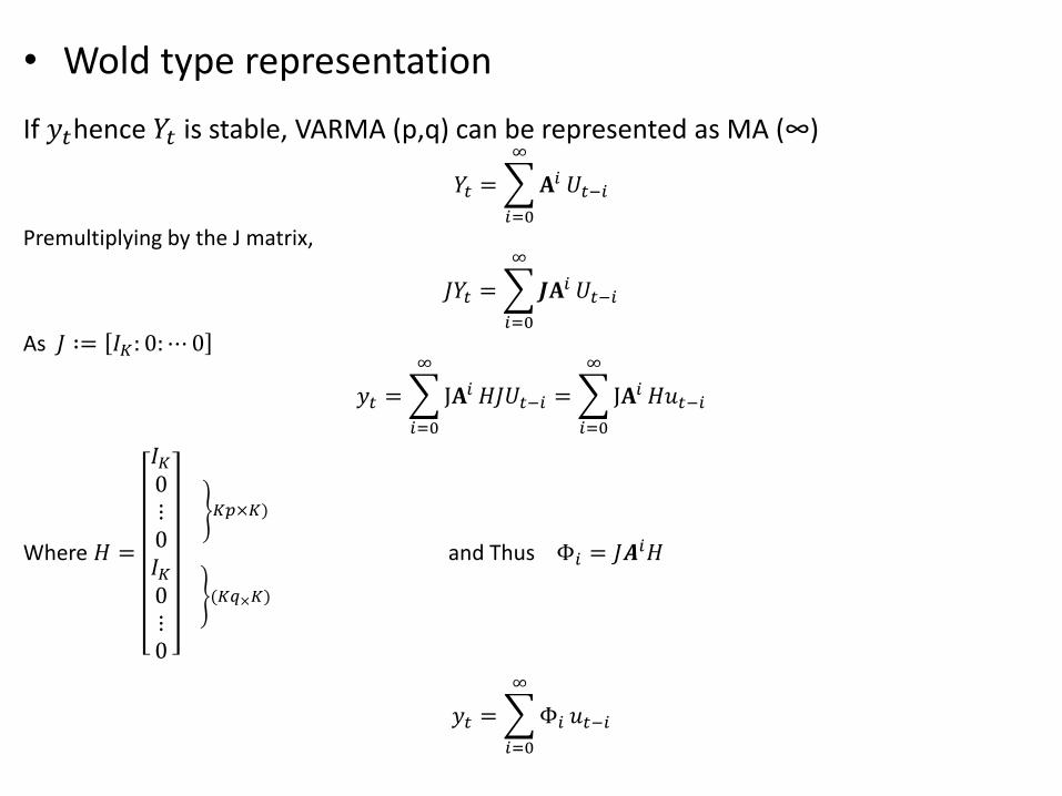
• Wold type representation
If 𝑦𝑡hence 𝑌𝑡 is stable, VARMA (p,q) can be represented as MA (∞)
𝑌𝑡 = 𝐀𝑖∞
𝑖=0
𝑈𝑡−𝑖
Premultiplying by the J matrix,
𝐽𝑌𝑡 = 𝑱𝐀𝑖∞
𝑖=0
𝑈𝑡−𝑖
As 𝐽 ∶= 𝐼𝐾: 0:⋯ 0
𝑦𝑡 = J𝐀𝑖∞
𝑖=0
𝐻𝐽𝑈𝑡−𝑖 = J𝐀𝑖∞
𝑖=0
𝐻𝑢𝑡−𝑖
Where 𝐻 =
𝐼𝐾0⋮0𝐼𝐾0⋮0
𝐾𝑝×𝐾)
(𝐾𝑞×𝐾)
and Thus Φ𝑖 = 𝐽𝑨𝑖𝐻
𝑦𝑡 = Φ𝑖
∞
𝑖=0
𝑢𝑡−𝑖
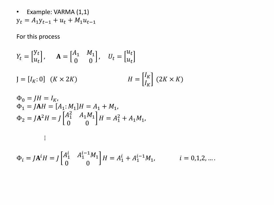
• Example: VARMA (1,1) y𝑡 = 𝐴1y𝑡−1 + 𝑢𝑡 +𝑀1𝑢𝑡−1 For this process
𝑌𝑡 =y𝑡𝑢𝑡
, 𝐀 =𝐴1 𝑀1
0 0, 𝑈𝑡 =
𝑢𝑡𝑢𝑡
J = 𝐼𝐾: 0 (𝐾 × 2𝐾) 𝐻 =𝐼𝐾𝐼𝐾
(2𝐾 × 𝐾)
Φ0 = 𝐽𝐻 = 𝐼𝐾 , Φ1 = 𝐽𝐀𝐻 = 𝐴1:𝑀1 𝐻 = 𝐴1 +𝑀1,
Φ2 = 𝐽𝐀2𝐻 = 𝐽 𝐴12 𝐴1𝑀1
0 0𝐻 = 𝐴1
2 + 𝐴1𝑀1,
⋮
Φ𝑖 = 𝐽𝐀𝑖𝐻 = 𝐽 𝐴1𝑖 𝐴1
𝑖−1𝑀1
0 0𝐻 = 𝐴1
𝑖 + 𝐴1𝑖−1𝑀1, 𝑖 = 0,1,2, … .
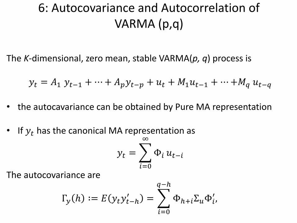
6: Autocovariance and Autocorrelation of VARMA (p,q)
The K-dimensional, zero mean, stable VARMA(p, q) process is
𝑦𝑡 = 𝐴1 𝑦𝑡−1 +⋯+ 𝐴𝑝𝑦𝑡−𝑝 + 𝑢𝑡 +𝑀1𝑢𝑡−1 +⋯+𝑀𝑞 𝑢𝑡−𝑞
• the autocavariance can be obtained by Pure MA representation • If 𝑦𝑡 has the canonical MA representation as
𝑦𝑡 = Φ𝑖
∞
𝑖=0
𝑢𝑡−𝑖
The autocovariance are
Γ𝑦 ℎ ∶= 𝐸 𝑦𝑡𝑦𝑡−ℎ′ = Φℎ+𝑖Σ𝑢Φ𝑖
′,
𝑞−ℎ
𝑖=0
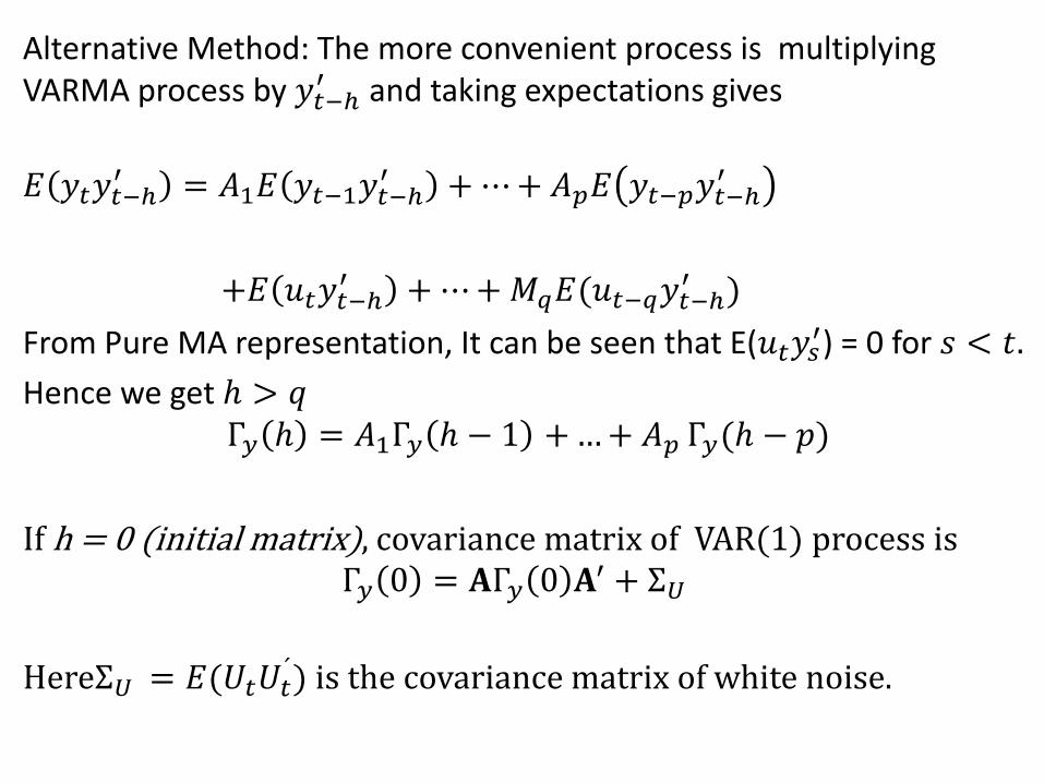
Alternative Method: The more convenient process is multiplying VARMA process by 𝑦𝑡−ℎ
′ and taking expectations gives
𝐸 𝑦𝑡𝑦𝑡−ℎ
′ = 𝐴1𝐸 𝑦𝑡−1𝑦𝑡−ℎ′ +⋯+ 𝐴𝑝𝐸 𝑦𝑡−𝑝𝑦𝑡−ℎ
′
+𝐸 𝑢𝑡𝑦𝑡−ℎ′ +⋯+𝑀𝑞𝐸(𝑢𝑡−𝑞𝑦𝑡−ℎ
′ )
From Pure MA representation, It can be seen that E(𝑢𝑡𝑦𝑠′) = 0 for 𝑠 < 𝑡.
Hence we get ℎ > 𝑞 Γ𝑦 ℎ = 𝐴1Γ𝑦 ℎ − 1 +…+ 𝐴𝑝 Γ𝑦(ℎ − 𝑝)
If h = 0 (initial matrix), covariance matrix of VAR(1) process is Γ𝑦 0 = 𝐀Γ𝑦 0 𝐀′ + Σ𝑈
HereΣ𝑈 = 𝐸(𝑈𝑡𝑈𝑡´) is the covariance matrix of white noise.
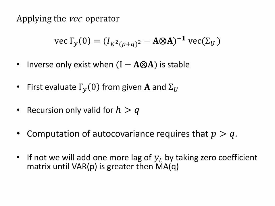
Applying the vec operator
vec Γ𝑦 0 = (𝐼𝐾2(𝑝+𝑞)2 − 𝐀⨂𝐀)−𝟏 vec(Σ𝑈 )
• Inverse only exist when (I − 𝐀⨂𝐀) is stable
• First evaluate Γ𝑦 0 from given 𝐀 and Σ𝑈
• Recursion only valid for ℎ > 𝑞
• Computation of autocovariance requires that 𝑝 > 𝑞.
• If not we will add one more lag of 𝑦𝑡 by taking zero coefficient matrix until VAR(p) is greater then MA(q)
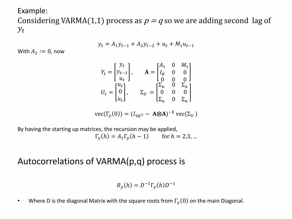
Example: Considering VARMA(1,1) process as p = q so we are adding second lag of 𝑦𝑡
𝑦𝑡 = 𝐴1𝑦𝑡−1 + 𝐴2𝑦𝑡−2 + 𝑢𝑡 +𝑀1𝑢𝑡−1 With 𝐴2 ∶= 0, now
𝑌𝑡 =
𝑦𝑡𝑦𝑡−1𝑢𝑡
, 𝐀 =𝐴1 0 𝑀1
𝐼𝐾 0 00 0 0
𝑈𝑡 =
𝑢𝑡0𝑢𝑡
, Σ𝑈 =Σ𝑢 0 Σ𝑢 0 0 0Σ𝑢 0 Σ𝑢
vec(Γ𝑦 0 ) = (𝐼9𝐾2 − 𝐀⨂𝐀)−𝟏 vec(Σ𝑈 )
By having the starting up matrices, the recursion may be applied,
Γ𝑦 ℎ = 𝐴1Γ𝑦 ℎ − 1 for ℎ = 2,3, …
Autocorrelations of VARMA(p,q) process is
𝑅𝑦 ℎ = 𝐷−1Γ𝑦 ℎ 𝐷−1
• Where D is the diagonal Matrix with the square roots from Γ𝑦 0 on the main Diagonal.
References
• Hannan, E. J. & Deistler, M. (1988). ´´The Statistical Theory of Linear Systems’’, JohnWiley, New York.
• Lutkepohl, H. (2005). ´´New Introduction to Multiple Time Series Analysis´´, Springer, Berlin.
• Wei, W. W. S. (2005) ``Time Series Analysis: Univariate and Multivariate Methods`` Second Edition, Pearson (Addison Wesley)

Thank You