Operator-valued Kernel-based Vector Autoregressive

Models for Network Inference

Nehemy Lim, Florence D’Alche-Buc, Cedric Auliac, George Michailidis

To cite this version:

Nehemy Lim, Florence D’Alche-Buc, Cedric Auliac, George Michailidis. Operator-valuedKernel-based Vector Autoregressive Models for Network Inference. 2014. <hal-00872342v2>

HAL Id: hal-00872342

https://hal.archives-ouvertes.fr/hal-00872342v2

Submitted on 10 Mar 2014

HAL is a multi-disciplinary open accessarchive for the deposit and dissemination of sci-entific research documents, whether they are pub-lished or not. The documents may come fromteaching and research institutions in France orabroad, or from public or private research centers.

L’archive ouverte pluridisciplinaire HAL, estdestinee au depot et a la diffusion de documentsscientifiques de niveau recherche, publies ou non,emanant des etablissements d’enseignement et derecherche francais ou etrangers, des laboratoirespublics ou prives.

Operator-valued Kernel-based Vector

Autoregressive Models for Network Inference

Nehemy Lim

IBISC EA 4526, Universite d’Evry-Val d’Essonne,

23 Bd de France, 91000,Evry, France,

and CEA, LIST, 91191 Gif-sur-Yvette CEDEX, France,

Florence d’Alche-Buc

INRIA-Saclay, LRI umr CNRS 8623, Universite Paris Sud, France

and IBISC EA 4526, Universite d’Evry-Val d’Essonne

Cedric Auliac

CEA, LIST, 91191 Gif-sur-Yvette CEDEX, France,

George Michailidis

Department of Statistics, University of Michigan,

Ann Arbor, MI 48109-1107

February 14, 2014

Abstract

Reverse-modeling of dynamical systems from time-course data still re-mains a challenging and canonical problem in knowledge discovery. Forthis learning task, a number of approaches primarily based on sparse linearmodels or Granger causality have been proposed in the literature. How-ever when the dynamics are nonlinear, there does not exist a systematicanswer that takes into account the nature of the underlying system. Weintroduce a novel family of vector autoregressive models based on differ-ent operator-valued kernels to identify the dynamical system and retrievethe target network. As in the linear case, a key issue is to control themodel’s sparsity. This control is performed through the joint learning ofthe structure of the kernel and the basis vectors. To solve this learningtask, we propose an alternating optimization algorithm based on proxi-mal gradient procedures that learn both the structure of the kernel andthe basis vectors. Results on the DREAM3 competition gene regulatorybenchmark networks of size 10 and 100 show the new model outperformsexisting methods.

1

1 Introduction

In many scientific problems, high dimensional data with network structure play akey role in knowledge discovery (Kolaczyk, 2009). For example, recent advancesin high throughput technologies have facilitated the simultaneous study of com-ponents of complex biological systems. Hence, molecular biologists are able tomeasure the expression levels of the entire genome and a good portion of theproteome and metabolome under different conditions and thus gain insight onhow organisms respond to their environment. For this reason, reconstruction ofgene regulatory networks from expression data has become a canonical problemin computational systems biology (Lawrence et al, 2010). Similar data struc-tures emerge in other scientific domains. For instance, political scientists havefocused on the analysis of roll call data of legislative bodies, since they allowthem to study party cohesion and coalition formation through the underlyingnetwork reconstruction (Morton and Williams, 2010), while economists havefocused on understanding companies creditworthiness or contagion (Gilchristet al, 2009). Understanding climate changes implies to be able to predict thebehavior of climate variables and their dependence relationship (Parry et al,2007; Liu et al, 2010). Two classes of network inference problems have emergedsimultaneously from all these fields: the inference of association networks thatrepresent coupling between variables of interest (Meinshausen and Buhlmann,2006; Kramer et al, 2009) and the inference of “causal” networks that describehow variables influence other ones (Murphy, 1998; Perrin et al, 2003; Auliacet al, 2008; Zou and Feng, 2009; Shojaie and Michailidis, 2010; Maathuis et al,2010; Bolstad et al, 2011; Dondelinger et al, 2013; Chatterjee et al, 2012).

Over the last decade, a number of statistical techniques have been intro-duced for estimating networks from high-dimensional data in both cases. Theydivide into model-free and model-driven approaches. Model-free approaches forassociation networks directly estimate information-theoretic measures, such asmutual information to detect edges in the network (Hartemink, 2005; Margolinet al, 2006). Among model-driven approaches, graphical models have emergedas a powerful class of models and a lot of algorithmic and theoretical advanceshave occured for static (independent and identically distributed) data under theassumption of sparsity. For instance, Gaussian graphical models have been thor-oughly studied (see Buhlmann and van de Geer (2011) and references therein)under different regularization schemes to reinforce sparsity in linear models inan unstructured or a structured way. In order to infer causal relationship net-works, Bayesian networks (Friedman, 2004; Lebre, 2009) have been developed ei-ther from static data or time-series within the framework of dynamical Bayesiannetworks. In the case of continuous variables, linear multivariate autoregressivemodeling (Michailidis and d’Alche Buc, 2013) has been developed with again animportant focus on sparse models. In this latter framework, Granger causalitymodels have attracted an increasing interest to capture causal relationships.

However, little work has focused on network inference for continuous vari-ables in the presence of nonlinear dynamics despite the fact that regulatorymechanisms involve such dynamics. Of special interest are approaches based on

2

parametric ordinary differential equations (Chou and Voit, 2009) that alterna-tively learn the structure of the model and its parameters. The most successfulapproaches decompose into Bayesian Learning (Mazur et al, 2009; Aijo andLahdesmaki, 2009) that allows to deal with stochasticity of the biological data,while easily incorporating prior knowledge and genetic programming (Iba, 2008)that provides a population-based algorithm for a stochastic search in the struc-ture space. In this study, we start from a regularization theory perspective andintroduce a general framework for nonlinear multivariate modeling and networkinference. Our aim is to extend the framework of sparse linear modeling tothat of sparse nonlinear modeling. In the machine learning community, a pow-erful tool to extend linear models to nonlinear ones is based on kernels. Thefamous kernel trick allows to deal with nonlinear learning problems by workingimplicitly in a new feature space, where inner products can be computed usinga symmetric positive semi-definite function of two variables, called a kernel. Inparticular, a given kernel allows to build a unique Reproducing Kernel HilbertSpace (RKHS), e.g. a functional space where regularized models can be definedfrom data using representer theorems. The RKHS theory provides a unifiedframework for many kernel-based models and a principled way to build new(nonlinear) models. Since multivariate time-series modeling requires definingvector-valued models, we propose to build on operator-valued kernels and theirassociated reproducing kernel Hilbert space theory (Senkene and Tempel’man,1973) that were recently introduced in machine learning by Micchelli and Pontil(2005) for the multi-task learning problem with vector-valued functions. Amongdifferent ongoing research on the subject (Alvarez et al, 2011), new applicationsconcern vector field regression (Baldassarre et al, 2010), structured classifica-tion (Dinuzzo and Fukumizu, 2011), functional regression (Kadri et al, 2011)and link prediction (Brouard et al, 2011). However, their use in the context oftime series is novel.

Building upon our previous work (Lim et al, 2013) that focused on a specificmodel, we define a whole family of nonlinear vector autoregressive models basedon various operator-valued kernels. Once an operator-valued kernel-based modelis learnt, we compute an empirical estimate of its Jacobian, providing a genericand simple way to extract dependence relationship among variables. We discusshow a chosen operator-valued kernel can produce not only a good approximationof the systems dynamics, but also a flexible and controllable Jacobian estimate.To obtain sparse networks and get sparse Jacobian estimates, we extend thesparsity constraint applied to the design matrix regularly employed in linearmodeling. To control smoothness of the model, the definition of the loss functioninvolves an ℓ2-norm penalty and additionally, may include two different kindsof penalties, depending on the nature of the estimation problem: an ℓ1 penaltythat imposes sparsity to the whole matrix of parameter vectors, suitable whenthe main goal is to ensure sparsity of the Jacobian, and a mixed ℓ1/ℓ2-norm thatallows one to deal with an unfavorable ratio between the network size and thelength of observed time-series. To optimize a loss function that contains thesenon-differentiable terms, we develop a general proximal gradient algorithm.

Note that selected operator-valued kernels involve a positive semi-definite

3

matrix as a hyperparameter. The background knowledge required for its def-inition is in general not available, especially in a network inference task. Toaddress this kernel design task together with the other parameters, we intro-duce an efficient strategy that alternatively learns the parameter vectors and thepositive semi-definite matrix that characterizes the kernel. This matrix plays animportant role regarding the Jacobian sparsity; the estimation procedure for thematrix parameter also involves an ℓ1 penalty and a positive semi-definitenessconstraint. We show that without prior knowledge on the relationship betweenvariables, the proposed algorithm is able to retrieve the network structure of agiven underlying dynamical system from the observation of its behavior throughtime.

The structure of the paper is as follows: in Section 2, we present the generalnetwork inference scheme. In Section 3, we recall elements of RKHS theorydevoted to vector-valued functions and introduce operator-valued kernel-basedautoregressive models. Section 4 presents the learning algorithm that estimatesboth the parameters of the model and the parameters of the kernel. Section 5illustrates the performance of the model and the algorithm through extensivenumerical work based on both synthetic and real data, and comparison withstate-of-the-art methods.

2 Network inference from nonlinear vector au-

toregressive models

Let xt ∈ Rd denote the observed state of a dynamical system comprising of

d state variables. We are interested in inferring direct influences of a statevariable j on other variables i 6= j, (i, j) ∈ 1, · · · , d2. The set of influencesamong state variables is encoded by a network matrix A = (aij) of size d×d forwhich a coefficient aij = 1 if the state variable j influences the state variable i,0 otherwise. Further, we assume that a first-order stationary model is adequateto capture the temporal evolution of the system under study, which can exhibitnonlinear dynamics captured by a function h : Rd → R

d:

xt+1 = h(xt) + ut (1)

where ut is a noise term.Some models such as linear models h(xt) = Bxt or parametric models,

explicitly involve a matrix that can be interpreted as a network matrix andits estimation (possibly sparse) can be directly accomplished. However, fornonlinear models this is a more involved task. Our strategy is to first learn hfrom the data and subsequently estimate A using the values of the instantaneousJacobian matrix of model h, measured at each time point. The underlying idea

is that partial derivatives ∂h(xt)i

∂xjt

reflects the influence of explanatory variable

j at time t on the value of the i-th model’s output h(xt)i. We interpret that if

∂h(xt)i

∂xjt

is high in absolute value, then variable j influences variable i. Several

4

estimators of A can be built from those partial derivatives. We propose to usethe empirical mean of the instantaneous Jacobian matrix of h. Specifically,denote by x1, . . . ,xN+1 the observed time series of the network state. Then,∀(i, j) ∈ 1, . . . , d2, an estimate J(h) of the Jacobian matrix ∇h = J(h) isgiven by:

J(h)ij =1

N

N∑

t=1

∂h(xt)i

∂xjt

(2)

In the remainder of the paper, we note J(h)ij the (i, j) coefficient of the em-

pirical mean of Jacobian of h and J(h)ij(t) its value at a given time t. Each

coefficient J(h)ij in absolute value gives a score to the potential influence ofvariable j on variable i. To provide a final estimate of A, these coefficients aresorted in increasing order and a rank matrix R is built according to the follow-

ing rule: let r(i, j) be the rank of the coefficient J(h)ij among the p(p+1)2 sorted

coefficients, then we define R, the rank matrix as: Rij = r(i, j).To get an estimate of A, coefficients of R are thresholded given a positive thresh-old θ: Aij = 1, if (Rij > θ), and 0, otherwise.

Note that to obtain a high quality estimate of the network, we need a class offunctions h whose Jacobian matrices can be controlled during learning in sucha way that they could provide good continuous approximators of A. In thiswork, we propose a new class of nonparametric vector autoregressive modelsthat exhibit such properties. Specifically, we introduce Operator-valued Kernel-based Vector AutoRegressive (OKVAR) models, that constitute a rich class asdiscussed in the next section.

3 Operator-valued kernels and vector autoregres-

sive models

3.1 From scalar-valued kernel to operator-valued kernel

models of autoregresssion

In order to solve the vector autoregression problem set in Eq. (1) with a nonlin-ear model, one option is to decompose it into d tasks and use, for each task i, ascalar-valued model hi such as a kernel-based model. Dataset DN now reducesinto d datasets of the form Di

N = (xℓ, xiℓ+1), ℓ = 1, . . . , N. Each task i is now

a regression task that we may solve by estimating a nonparametric model. Forinstance, kernel-based regression models are good candidates for those tasks.A unique feature of these approaches is that they can be derived from Repro-ducing Kernel Hilbert Space theory that offers a rigorous background for regu-larization. For instance, kernel-ridge regression and Support Vector Regressionprovide consistent estimator as soon as the chosen kernel is universal. Then, foreach i = 1, . . . , d, a model based on a positive definite kernel k : Rd × R

d → R

5

writes as:

hi(xt) =

N∑

ℓ=1

wiℓk(xℓ,xt), (3)

where wi is the parameter vector attached to model i. Although this decom-position is well justified when the covariance matrix of noise ut is diagonal, inthe general case, the d regression tasks are not independent. The purpose ofthis work is therefore to extend such approaches to the vector autoregressionproblem in order to provide (i), a general family of nonparametric models and(ii), suitable models for network inference by Jacobian estimation. We now aimto predict the state vector of a dynamical system xt+1 at time t + 1, given itsstate xt at time t using kernel-based models appropriate for vectors. As a vec-tor autoregressive model is a vector-valued function, the RKHS theory basedon scalar-valued kernel does not apply. However, if the kernel is chosen to beoperator-valued e.g. matrix-valued in our setting, then RKHS theory devotedto operator-valued kernel provides a similar framework to build models and tojustify their use. In the following, we introduce the basic building blocks ofoperator-valued kernel-based theory and notations to extend (3) into models ofthe following form:

h(xt) =

N∑

ℓ=1

K(xt,xℓ)wℓ, (4)

where K is an operator-valued kernel to be defined in next section and wℓ, ℓ =1, . . . , N are parameter vectors of dimension d.

3.2 RKHS theory for vector-valued functions

In RKHS theory with operator-valued kernels, we consider functions with inputin some set X and with vector values in some given Hilbert space Fy. Forcompleteness, we first describe the general framework and then come back tothe case of interest, namely X = Fy = R

d. Denote by L(Fy), the set of allbounded linear operators from Fy to itself. Given A ∈ L(Fy), A

∗ denotes itsadjoint. Then, an operator-valued kernel K is defined as follows:

Definition 1 (Operator-valued kernel) (Senkene and Tempel’man, 1973; Capon-netto et al, 2008)Let X be a set and Fy a Hilbert space. Then, K : X × X → L(Fy) is a kernelif:

• ∀ (x, z) ∈ X × X , K(x, z) = K(z,x)∗

• ∀m ∈ N, ∀(xi,yi), i = 1, . . . ,m ⊆ X ×Fy,∑m

i,j=1〈yi,K(xi,xj)yj〉Fy≥

0

When Fy = Rd, each kernel function is matrix-valued, which means that two

inputs x and z can be compared in more details. Moreover, Senkene and Tem-pel’man (1973); Micchelli and Pontil (2005) established that one can build a

6

unique RKHS HK from a given operator-valued kernel K. The RKHS HK isbuilt by taking the closure of spanK(·,x)y|x ∈ X ,y ∈ Fy endowed with thescalar product 〈f, g〉HK

=∑

i,j〈ui,K(ri, sj)vj〉Fywith f(·) =

∑

i K(·, ri)ui

and g(·) =∑

j K(·, sj)vj . The corresponding norm ‖ · ‖HKis defined by

‖ f ‖2HK= 〈f, f〉HK

.For the sake of notational simplicity, we omit K and use H = HK in the

remainder of the paper. As in the scalar case, one of the most appealing featuresof RKHS is to provide a theoretical framework for regularization, e.g. represen-ter theorems. Let us consider the case of regression with a convex loss functionV . We denote by DN = (xℓ,yℓ), ℓ = 1, . . . , N ⊆ X × Fy the data set underconsideration.

Theorem 1 ((Micchelli and Pontil, 2005)) Let V be some prescribed lossfunction, and λ > 0 the regularization parameter. Then, any minimizer of thefollowing optimization problem:

argminh∈H

L(h) =N∑

ℓ=1

V (h(xℓ),yℓ) + λ‖h‖2H ,

admits an expansion:

h(·) =N∑

ℓ=1

K(·,xℓ)cℓ , (5)

where the coefficients cℓ, ℓ = 1, · · · , N are vectors in the Hilbert space Fy.

Such a result justifies a new family of models of the form (5) for vectorregression in R

d. Then, the operator-valued kernel (OVK) becomes a matrix-valued one. In case this matrix is diagonal, the model reduces to d independentmodels with scalar outputs and there is no need for a matrix-valued kernel.In other cases, when we assume that the different components of the vector-valued function are not independent and may share some underlying structure, anon-diagonal matrix-valued kernel allows to take into consideration similaritiesbetween the components of the input vectors. Initial applications of matrix-valued kernels deal with structured output regression tasks, such as multi-tasklearning and structured classification. In the following, we propose to applythis framework to autoregression. We examine different matrix-valued kernelsas well as different loss functions and discuss about their relevance for networkinference.

3.3 The OKVAR family

Let now fix X = Fy = Rd. Recall that the objective is to estimate an vector au-

toregressive model. Given the observed d−dimensional time series x1, . . . ,xN+1

that we use as the training dataset DN = (x1,x2), . . . , (xN ,xN+1), the non-parametric model h is defined as

h(xt;DN ) =

N∑

ℓ=1

K(xt,xℓ)cℓ (6)

7

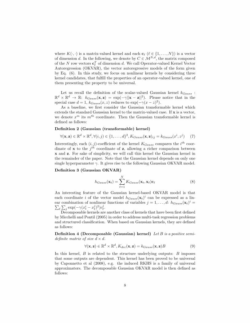
where K(·, ·) is a matrix-valued kernel and each cℓ (ℓ ∈ 1, . . . , N) is a vectorof dimension d. In the following, we denote by C ∈MN,d, the matrix composedof the N row vectors cTℓ of dimension d. We call Operator-valued Kernel VectorAutoregression (OKVAR), the vector autoregressive models of the form givenby Eq. (6). In this study, we focus on nonlinear kernels by considering threekernel candidates, that fulfill the properties of an operator-valued kernel, one ofthem presenting the property to be universal.

Let us recall the definition of the scalar-valued Gaussian kernel kGauss :R

d × Rd → R: kGauss(x, z) = exp(−γ||x − z||2). Please notice that in the

special case d = 1, kGauss(x, z) reduces to exp(−γ(x− z)2).As a baseline, we first consider the Gaussian transformable kernel which

extends the standard Gaussian kernel to the matrix-valued case. If x is a vector,we denote xm its mth coordinate. Then the Gaussian transformable kernel isdefined as follows:

Definition 2 (Gaussian (transformable) kernel)

∀(x, z) ∈ Rd × R

d, ∀(i, j) ∈ 1, . . . , d2,KGauss(x, z)ij = kGauss(xi, zj) (7)

Interestingly, each (i, j)-coefficient of the kernel KGauss compares the ith coor-dinate of x to the jth coordinate of z, allowing a richer comparison betweenx and z. For sake of simplicity, we will call this kernel the Gaussian kernel inthe remainder of the paper. Note that the Gaussian kernel depends on only onesingle hyperparameter γ. It gives rise to the following Gaussian OKVAR model.

Definition 3 (Gaussian OKVAR)

hGauss(xt) =

N∑

ℓ=1

KGauss(xt,xℓ)cℓ (8)

An interesting feature of the Gaussian kernel-based OKVAR model is thateach coordinate i of the vector model hGauss(xt)

i can be expressed as a lin-ear combination of nonlinear functions of variables j = 1, . . . , d: hGauss(xt)

i =∑

ℓ

∑

j exp(−γ(xit − xj

ℓ)2)cjℓ .

Decomposable kernels are another class of kernels that have been first definedby Micchelli and Pontil (2005) in order to address multi-task regression problemsand structured classification. When based on Gaussian kernels, they are definedas follows:

Definition 4 (Decomposable (Gaussian) kernel) Let B is a positive semi-definite matrix of size d× d.

∀(x, z) ∈ Rd × R

d,Kdec(x, z) = kGauss(x, z)B (9)

In this kernel, B is related to the structure underlying outputs: B imposesthat some outputs are dependent. This kernel has been proved to be universalby Caponnetto et al (2008), e.g. the induced RKHS is a family of universalapproximators. The decomposable Gaussian OKVAR model is then defined asfollows:

8

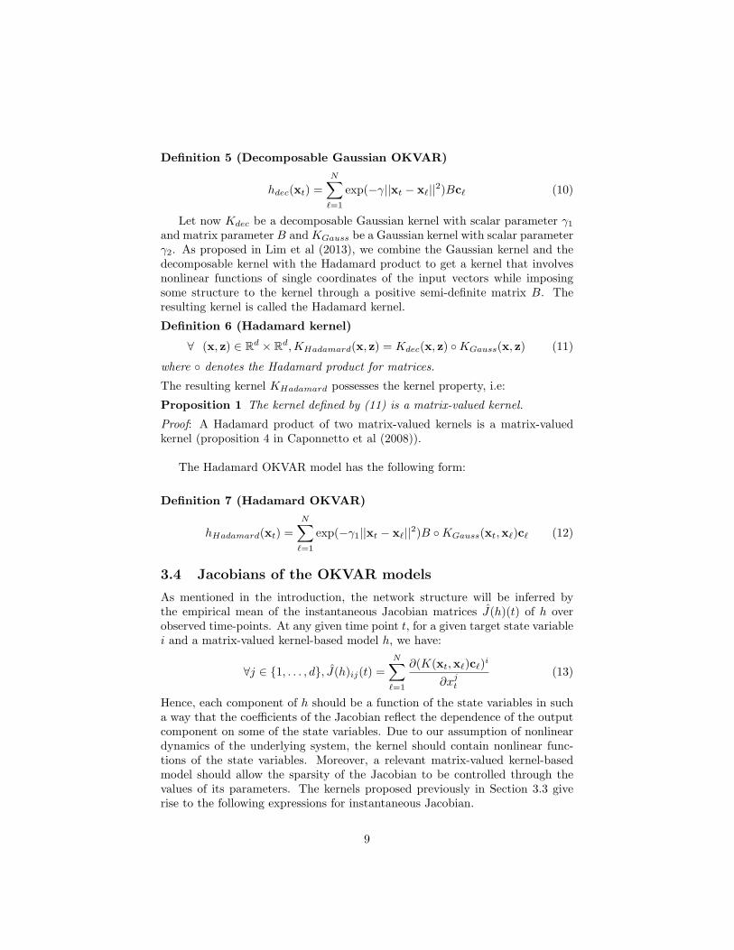
Definition 5 (Decomposable Gaussian OKVAR)

hdec(xt) =

N∑

ℓ=1

exp(−γ||xt − xℓ||2)Bcℓ (10)

Let now Kdec be a decomposable Gaussian kernel with scalar parameter γ1and matrix parameter B andKGauss be a Gaussian kernel with scalar parameterγ2. As proposed in Lim et al (2013), we combine the Gaussian kernel and thedecomposable kernel with the Hadamard product to get a kernel that involvesnonlinear functions of single coordinates of the input vectors while imposingsome structure to the kernel through a positive semi-definite matrix B. Theresulting kernel is called the Hadamard kernel.

Definition 6 (Hadamard kernel)

∀ (x, z) ∈ Rd × R

d,KHadamard(x, z) = Kdec(x, z) KGauss(x, z) (11)

where denotes the Hadamard product for matrices.

The resulting kernel KHadamard possesses the kernel property, i.e:

Proposition 1 The kernel defined by (11) is a matrix-valued kernel.

Proof: A Hadamard product of two matrix-valued kernels is a matrix-valuedkernel (proposition 4 in Caponnetto et al (2008)).

The Hadamard OKVAR model has the following form:

Definition 7 (Hadamard OKVAR)

hHadamard(xt) =

N∑

ℓ=1

exp(−γ1||xt − xℓ||2)B KGauss(xt,xℓ)cℓ (12)

3.4 Jacobians of the OKVAR models

As mentioned in the introduction, the network structure will be inferred bythe empirical mean of the instantaneous Jacobian matrices J(h)(t) of h overobserved time-points. At any given time point t, for a given target state variablei and a matrix-valued kernel-based model h, we have:

∀j ∈ 1, . . . , d, J(h)ij(t) =N∑

ℓ=1

∂(K(xt,xℓ)cℓ)i

∂xjt

(13)

Hence, each component of h should be a function of the state variables in sucha way that the coefficients of the Jacobian reflect the dependence of the outputcomponent on some of the state variables. Due to our assumption of nonlineardynamics of the underlying system, the kernel should contain nonlinear func-tions of the state variables. Moreover, a relevant matrix-valued kernel-basedmodel should allow the sparsity of the Jacobian to be controlled through thevalues of its parameters. The kernels proposed previously in Section 3.3 giverise to the following expressions for instantaneous Jacobian.

9

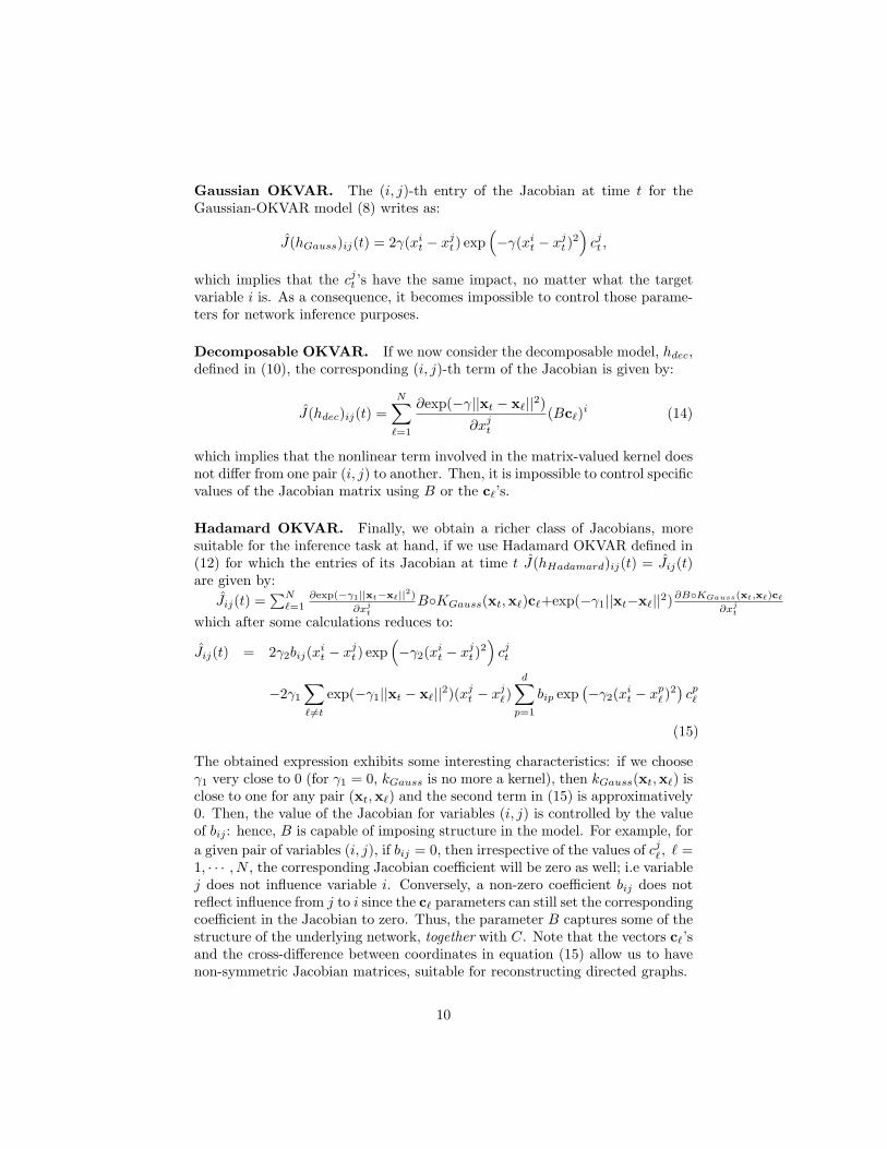
Gaussian OKVAR. The (i, j)-th entry of the Jacobian at time t for theGaussian-OKVAR model (8) writes as:

J(hGauss)ij(t) = 2γ(xit − xj

t ) exp(

−γ(xit − xj

t )2)

cjt ,

which implies that the cjt ’s have the same impact, no matter what the targetvariable i is. As a consequence, it becomes impossible to control those parame-ters for network inference purposes.

Decomposable OKVAR. If we now consider the decomposable model, hdec,defined in (10), the corresponding (i, j)-th term of the Jacobian is given by:

J(hdec)ij(t) =

N∑

ℓ=1

∂exp(−γ||xt − xℓ||2)∂xj

t

(Bcℓ)i (14)

which implies that the nonlinear term involved in the matrix-valued kernel doesnot differ from one pair (i, j) to another. Then, it is impossible to control specificvalues of the Jacobian matrix using B or the cℓ’s.

Hadamard OKVAR. Finally, we obtain a richer class of Jacobians, moresuitable for the inference task at hand, if we use Hadamard OKVAR defined in(12) for which the entries of its Jacobian at time t J(hHadamard)ij(t) = Jij(t)are given by:

Jij(t) =∑N

ℓ=1∂exp(−γ1||xt−xℓ||

2)

∂xjt

BKGauss(xt,xℓ)cℓ+exp(−γ1||xt−xℓ||2)∂BKGauss(xt,xℓ)cℓ

∂xjt

which after some calculations reduces to:

Jij(t) = 2γ2bij(xit − xj

t ) exp(

−γ2(xit − xj

t )2)

cjt

−2γ1∑

ℓ 6=t

exp(−γ1||xt − xℓ||2)(xjt − xj

ℓ)

d∑

p=1

bip exp(−γ2(xi

t − xpℓ )

2)cpℓ

(15)

The obtained expression exhibits some interesting characteristics: if we chooseγ1 very close to 0 (for γ1 = 0, kGauss is no more a kernel), then kGauss(xt,xℓ) isclose to one for any pair (xt,xℓ) and the second term in (15) is approximatively0. Then, the value of the Jacobian for variables (i, j) is controlled by the valueof bij : hence, B is capable of imposing structure in the model. For example, for

a given pair of variables (i, j), if bij = 0, then irrespective of the values of cjℓ , ℓ =1, · · · , N , the corresponding Jacobian coefficient will be zero as well; i.e variablej does not influence variable i. Conversely, a non-zero coefficient bij does notreflect influence from j to i since the cℓ parameters can still set the correspondingcoefficient in the Jacobian to zero. Thus, the parameter B captures some of thestructure of the underlying network, together with C. Note that the vectors cℓ’sand the cross-difference between coordinates in equation (15) allow us to havenon-symmetric Jacobian matrices, suitable for reconstructing directed graphs.

10

4 Learning OKVAR with proximal gradient al-

gorithms

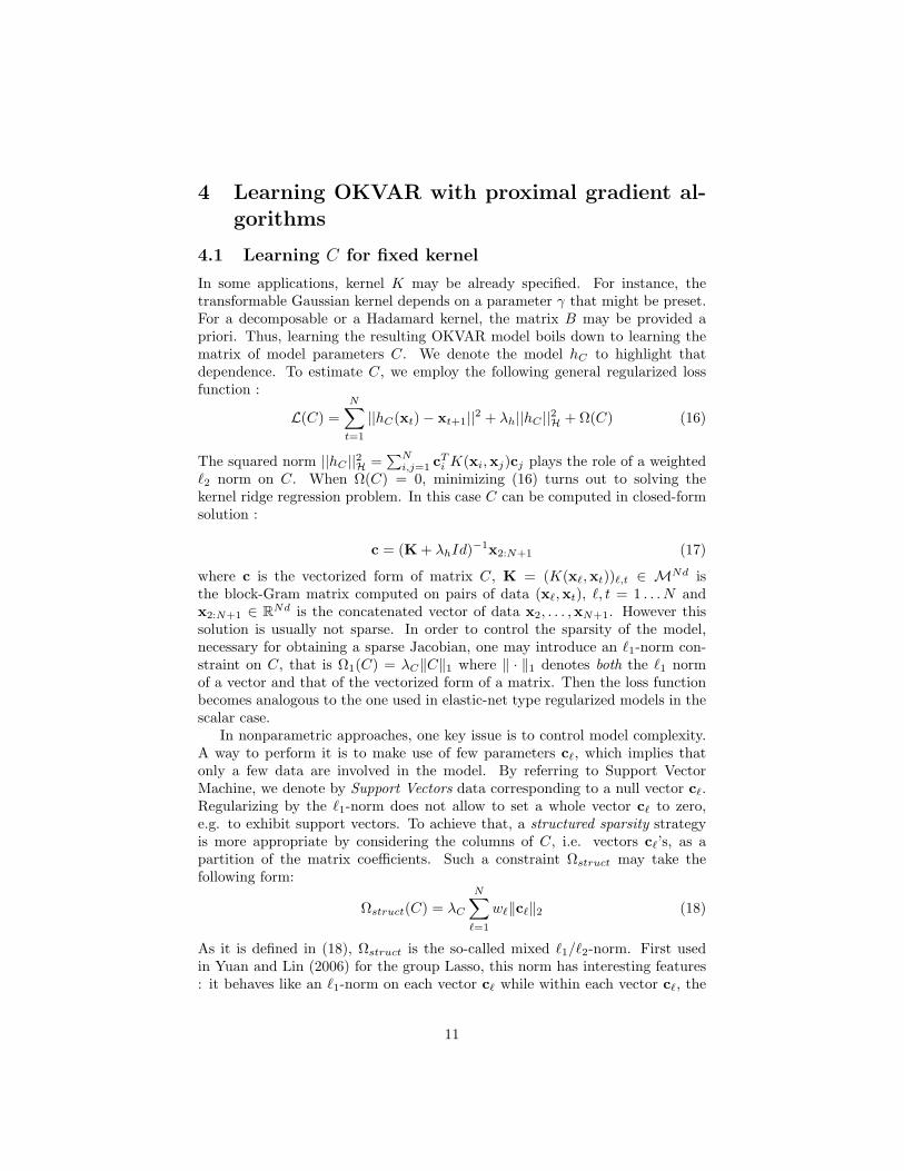
4.1 Learning C for fixed kernel

In some applications, kernel K may be already specified. For instance, thetransformable Gaussian kernel depends on a parameter γ that might be preset.For a decomposable or a Hadamard kernel, the matrix B may be provided apriori. Thus, learning the resulting OKVAR model boils down to learning thematrix of model parameters C. We denote the model hC to highlight thatdependence. To estimate C, we employ the following general regularized lossfunction :

L(C) =

N∑

t=1

||hC(xt)− xt+1||2 + λh||hC ||2H +Ω(C) (16)

The squared norm ||hC ||2H =∑N

i,j=1 cTi K(xi,xj)cj plays the role of a weighted

ℓ2 norm on C. When Ω(C) = 0, minimizing (16) turns out to solving thekernel ridge regression problem. In this case C can be computed in closed-formsolution :

c = (K+ λhId)−1x2:N+1 (17)

where c is the vectorized form of matrix C, K = (K(xℓ,xt))ℓ,t ∈ MNd isthe block-Gram matrix computed on pairs of data (xℓ,xt), ℓ, t = 1 . . . N andx2:N+1 ∈ R

Nd is the concatenated vector of data x2, . . . ,xN+1. However thissolution is usually not sparse. In order to control the sparsity of the model,necessary for obtaining a sparse Jacobian, one may introduce an ℓ1-norm con-straint on C, that is Ω1(C) = λC‖C‖1 where ‖ · ‖1 denotes both the ℓ1 normof a vector and that of the vectorized form of a matrix. Then the loss functionbecomes analogous to the one used in elastic-net type regularized models in thescalar case.

In nonparametric approaches, one key issue is to control model complexity.A way to perform it is to make use of few parameters cℓ, which implies thatonly a few data are involved in the model. By referring to Support VectorMachine, we denote by Support Vectors data corresponding to a null vector cℓ.Regularizing by the ℓ1-norm does not allow to set a whole vector cℓ to zero,e.g. to exhibit support vectors. To achieve that, a structured sparsity strategyis more appropriate by considering the columns of C, i.e. vectors cℓ’s, as apartition of the matrix coefficients. Such a constraint Ωstruct may take thefollowing form:

Ωstruct(C) = λC

N∑

ℓ=1

wℓ‖cℓ‖2 (18)

As it is defined in (18), Ωstruct is the so-called mixed ℓ1/ℓ2-norm. First usedin Yuan and Lin (2006) for the group Lasso, this norm has interesting features: it behaves like an ℓ1-norm on each vector cℓ while within each vector cℓ, the

11

coefficients are subject to an ℓ2-norm constraint. wℓ’s are positive weights whosevalues depend on the application. For instance, in our case, as the observedtime-course data are the response of a dynamical system to some given initialcondition, wℓ should increase with ℓ, meaning that we put emphasis on the firsttime-points.

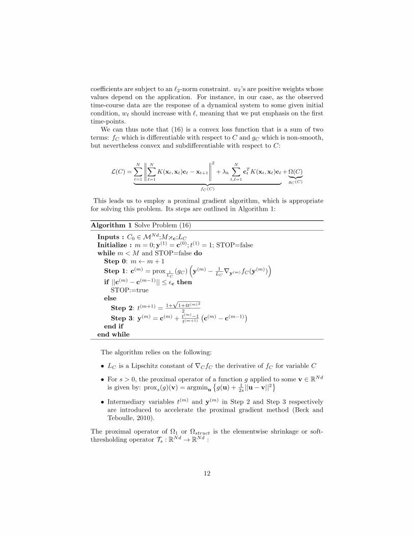
We can thus note that (16) is a convex loss function that is a sum of twoterms: fC which is differentiable with respect to C and gC which is non-smooth,but nevertheless convex and subdifferentiable with respect to C:

L(C) =

N∑

t=1

∥∥∥∥∥

N∑

ℓ=1

K(xt,xℓ)cℓ − xt+1

∥∥∥∥∥

2

+ λh

N∑

t,ℓ=1

cTt K(xt,xℓ)cℓ

︸ ︷︷ ︸

fC(C)

+Ω(C)︸ ︷︷ ︸

gC(C)

This leads us to employ a proximal gradient algorithm, which is appropriatefor solving this problem. Its steps are outlined in Algorithm 1:

Algorithm 1 Solve Problem (16)

Inputs : C0 ∈MNd;M ;ǫc;LC

Initialize : m = 0;y(1) = c(0); t(1) = 1; STOP=falsewhile m < M and STOP=false doStep 0: m← m+ 1

Step 1: c(m) = prox 1LC

(gC)(

y(m) − 1LC∇

y(m)fC(y(m))

)

if ||c(m) − c(m−1)|| ≤ ǫc thenSTOP:=true

else

Step 2: t(m+1) = 1+√

1+4t(m)2

2

Step 3: y(m) = c(m) + t(m)−1t(m+1)

(c(m) − c(m−1)

)

end ifend while

The algorithm relies on the following:

• LC is a Lipschitz constant of ∇CfC the derivative of fC for variable C

• For s > 0, the proximal operator of a function g applied to some v ∈ RNd

is given by: proxs(g)(v) = argminu

g(u) + 1

2s ||u− v||2

• Intermediary variables t(m) and y(m) in Step 2 and Step 3 respectivelyare introduced to accelerate the proximal gradient method (Beck andTeboulle, 2010).

The proximal operator of Ω1 or Ωstruct is the elementwise shrinkage or soft-thresholding operator Ts : RNd → R

Nd :

12

Let G be a partition of the indices of v, for a given subset of indices I ∈ G,

Ts(v)I =

(

1− s

‖vI‖2

)

+

vI

where vI ∈ R|I| denotes the coefficients of v indexed by I. Then, the proximal

gradient term in the mth iteration is given by:

prox 1LC

(gC)

(

y(m) − 1

LC∇

y(m)fC(y(m))

)

Iℓ

= Tsℓ(

y(m) − 1

LC∇

y(m)fC(y(m))

)

Iℓ

For gC = Ωstruct, sℓ = λCwℓ

LCand Iℓ, ℓ = 1, . . . , N is the subset of indices

corresponding to the ℓ-th column of C, while for gC = Ω1, sℓ =λC

LCand Iℓ, ℓ =

1, . . . , Nd is a singleton corresponding to a single entry of C.We also need to calculate LC a Lipschitz constant of ∇Cf . We can notice

that fC(C) can be rewritten as:

fC(C) = ‖Kc− x2:N+1‖2 + λhcTKc

Hence,∇CfC(C) = 2K([K+ λhId]c− x2:N+1)

Using some algebra, we can establish that:For c1, c2 ∈ R

Nd,

||∇CfC(c1)−∇CfC(c2)|| ≤ 2ρ(K2 + λhK

)

︸ ︷︷ ︸

LC

‖c1 − c2‖

where ρ(K2 + λhK), is the largest eigenvalue of K2 + λhK.Remark : It is of interest to notice that Algorithm 1 is very general and maybe used as long as the loss function can be split into two convex terms, one ofwhich is differentiable.

4.2 Learning C and the kernel

Other applications require the learning of kernel K. For instance, in order totackle the network inference task, one may choose a Gaussian decomposablekernel Kdec or a Gaussian transformable kernel KHadamard. When bandwidthparameters γ are preset, the positive semi-definite matrix B underlying thesekernels imposes structure in the model and has to be learnt. This leads to themore involved task of simultaneously learning the matrix of the model param-eters C as well as B. Thus, we aim to minimize the following loss function forthe two models hdec and hHadamard:

L(B,C) =

N∑

t=1

||hB,C(xt)− xt+1||2 + λh||hB,C ||2H +Ω(C) + Ω(B) (19)

13

with Ω(C) a sparsity-inducing norm (Ω1 or Ωstruct), Ω(B) = λB ||B||1 andsubject to the constraint that B ∈ S+d where S+d denotes the cone of positivesemi-definite matrices of size d × d. For fixed C, the squared norm of hB,C

imposes a smoothing constraint on B, while the ℓ1 norm of B aids in controllingthe sparsity of the model and its Jacobian.

Further, for fixed B, the loss function L(Bfixed, C) is convex in C and con-versely, for fixed C, L(B,Cfixed) is convex in B. We propose an alternatingoptimization scheme to minimize the overall loss L(B,C). Since both loss func-tions L(Bfixed, C) and L(B,Cfixed) involve a sum of two terms, one being dif-ferentiable and the other being sub-differentiable, we employ proximal gradientalgorithms to achieve the minimization.

For fixed B, the loss function becomes:

L(B, C) =

N∑

t=1

||hB,C(xt)− xt+1||2 + λh||hB,C ||2H +Ω(C), (20)

while for given C, it is given by:

L(B, C) =

N∑

t=1

||hB,C(xt)− xt+1||2 + λh||hB,C ||2H + λB ||B||1 (21)

In summary, the general form of the algorithm is given in Algorithm 2.

Algorithm 2 Solve Problem (19)

Inputs : B0 ∈ S+d ; ǫB ; ǫCInitialize : m = 0; STOP=falsewhile STOP=false do

Step 1: Given Bm, minimize the loss function (20) and obtain Cm

Step 2: Given Cm, minimize the loss function (21) and obtain Bm+1

if m > 0 thenSTOP:=||Bm −Bm−1|| ≤ ǫB and ||Cm − Cm−1|| ≤ ǫC

end ifStep 3: m← m+ 1

end while

At iteration m, Bm is fixed, kernel K is thus defined. Hence, estimation ofCm in Step 1 boils down to applying Algorithm 1 to minimize (20).

4.2.1 Learning the matrix B for fixed C

For given parameter matrix C, the loss function L(B, C) is minimized subjectto the constraint that B is positive semi-definite.

L(B, C) =

N∑

t=1

||hB,C(xt)− xt+1||2 + λh||hB,C ||2H︸ ︷︷ ︸

fB(B)

+λB ||B||1︸ ︷︷ ︸

g1,B(B)

+1S+d(B)

︸ ︷︷ ︸

g2,B(B)

(22)

14

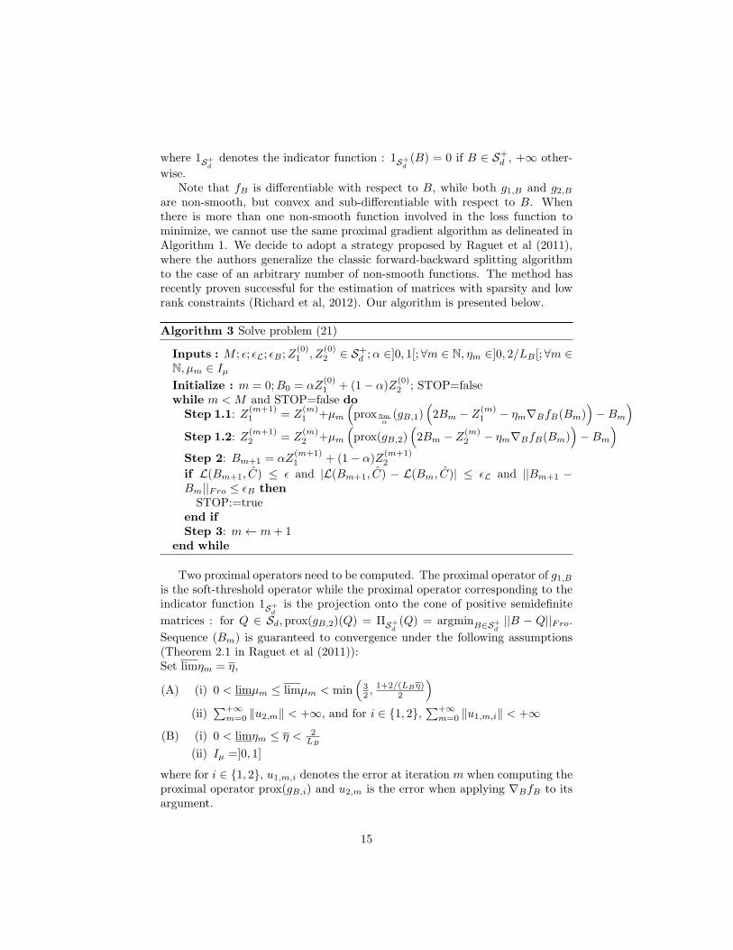
where 1S+d

denotes the indicator function : 1S+d(B) = 0 if B ∈ S+d , +∞ other-

wise.Note that fB is differentiable with respect to B, while both g1,B and g2,B

are non-smooth, but convex and sub-differentiable with respect to B. Whenthere is more than one non-smooth function involved in the loss function tominimize, we cannot use the same proximal gradient algorithm as delineated inAlgorithm 1. We decide to adopt a strategy proposed by Raguet et al (2011),where the authors generalize the classic forward-backward splitting algorithmto the case of an arbitrary number of non-smooth functions. The method hasrecently proven successful for the estimation of matrices with sparsity and lowrank constraints (Richard et al, 2012). Our algorithm is presented below.

Algorithm 3 Solve problem (21)

Inputs : M ; ǫ; ǫL; ǫB ;Z(0)1 , Z

(0)2 ∈ S+d ;α ∈]0, 1[; ∀m ∈ N, ηm ∈]0, 2/LB [; ∀m ∈

N, µm ∈ Iµ

Initialize : m = 0;B0 = αZ(0)1 + (1− α)Z

(0)2 ; STOP=false

while m < M and STOP=false doStep 1.1: Z

(m+1)1 = Z

(m)1 +µm

(

prox ηmα(gB,1)

(

2Bm − Z(m)1 − ηm∇BfB(Bm)

)

−Bm

)

Step 1.2: Z(m+1)2 = Z

(m)2 +µm

(

prox(gB,2)(

2Bm − Z(m)2 − ηm∇BfB(Bm)

)

−Bm

)

Step 2: Bm+1 = αZ(m+1)1 + (1− α)Z

(m+1)2

if L(Bm+1, C) ≤ ǫ and |L(Bm+1, C) − L(Bm, C)| ≤ ǫL and ||Bm+1 −Bm||Fro ≤ ǫB thenSTOP:=true

end ifStep 3: m← m+ 1

end while

Two proximal operators need to be computed. The proximal operator of g1,Bis the soft-threshold operator while the proximal operator corresponding to theindicator function 1S+

dis the projection onto the cone of positive semidefinite

matrices : for Q ∈ Sd, prox(gB,2)(Q) = ΠS+d(Q) = argminB∈S+

d||B − Q||Fro.

Sequence (Bm) is guaranteed to convergence under the following assumptions(Theorem 2.1 in Raguet et al (2011)):Set limηm = η,

(A) (i) 0 < limµm ≤ limµm < min(

32 ,

1+2/(LBη)2

)

(ii)∑+∞

m=0 ‖u2,m‖ < +∞, and for i ∈ 1, 2,∑+∞

m=0 ‖u1,m,i‖ < +∞

(B) (i) 0 < limηm ≤ η < 2LB

(ii) Iµ =]0, 1]

where for i ∈ 1, 2, u1,m,i denotes the error at iteration m when computing theproximal operator prox(gB,i) and u2,m is the error when applying ∇BfB to itsargument.

15

This algorithm also makes use of the following gradient computations. Herewe present the computations for kernel KHadamard, but all of them still hold fora decomposable kernel by setting KGauss = 1.

Specifically, we get:

• for ∂∂bij

∥∥∥hB,C(xt)− xt+1

∥∥∥

2

∂

∂bij

∥∥∥hB,C(xt)− xt+1

∥∥∥

2

=∂

∂bij

d∑

p=1

(

hB,C(xt)p − xp

t+1

)2

= 2

(N∑

ℓ=1

kGauss(xt,xℓ)KGauss(xt,xℓ)ijcjℓ

)(

hB,C(xt)i − xi

t+1

)

+2

(N∑

ℓ=1

kGauss(xt,xℓ)KGauss(xt,xℓ)jiciℓ

)(

hB,C(xt)j − xj

t+1

)

• for ∂∂bij||hB,C ||2H

∂

∂bij||hB,C ||2H =

∂

∂bij

N∑

t=1

N∑

ℓ=1

cTt KHadamard(xt,xℓ)cℓ

=

N∑

t=1

N∑

ℓ=1

citkGauss(xt,xℓ)KGauss(xt,xℓ)ijcjℓ + cjtkGauss(xt,xℓ)KGauss(xt,xℓ)jic

iℓ

We again need to compute a Lipschitz constant LB for ∇BfB(B). After somecalculations, one can show the following inequality :For B1, B2 ∈ S+d ,

‖∇BfB(B1)−∇BfB(B2)‖2Fro ≤ L2B ‖B1 −B2‖2Fro

with

L2B = 4

d∑

i,j=1

(N∑

t=1

(N∑

ℓ=1

kGauss(xt,xℓ)KGauss(xt,xℓ)ijcjℓ

)(N∑

ℓ=1

d∑

q=1

kGauss(xt,xℓ)KGauss(xt,xℓ)iqcqℓ

)

+

N∑

t=1

(N∑

ℓ=1

kGauss(xt,xℓ)KGauss(xt,xℓ)jiciℓ

)(N∑

ℓ=1

d∑

q=1

kGauss(xt,xℓ)KGauss(xt,xℓ)jqcqℓ

))2

5 Results

5.1 Implementation

The performance of the developed OKVAR model family and the proposed op-timization algorithms were assessed on simulated data from a biological system

16

(DREAM3 challenge data set). These algorithms include a number of tuning

parameters. Specifically, in Algorithm 3, we set Z(0)1 = Z

(0)2 = B0 ∈ S+d , α = 0.5

and µm = 1. Parameters of the kernels were also fixed a priori : parameter γwas set to 0.2 for a transformable Gaussian kernel and to 0.1 for a decomposableGaussian kernel. In the case of a Hadamard kernel, two parameters need to bechosen : parameter γ2 of the transformable Gaussian kernel remains unchanged(γ2 = 0.2). On the other hand, as discussed in Section 3.4, parameter γ1 of thedecomposable Gaussian kernel is fixed to a low value (γ1 = 10−5) since it doesnot play a key role in the network inference task.

5.2 DREAM3 dataset

We start our investigation by considering data sets obtained from the DREAM3challenge (Prill et al, 2010). DREAM stands for Dialogue for Reverse Engi-neering Assessments and Methods (http://wiki.c2b2.columbia.edu/dream/index.php/The_DREAM_Project) and is a scientific consortium that organizeschallenges in computational biology and especially for gene regulatory networkinference. In a gene regulatory network, a gene i is said to regulate anothergene j if the expression of gene i at time t influences the expression of genej at time t + 1. The DREAM3 project provides realistic simulated data forseveral networks corresponding to different organisms (e.g. E. coli, Yeast, etc.)of different sizes and topological complexity. We focus here on size-10 and size-100 networks generated for the DREAM3 in-silico challenges. Each of thesenetworks corresponds to a subgraph of the currently accepted E. coli and S.cerevisiae gene regulatory networks and exhibits varying patterns of sparsityand topological structure. They are referred to as E1, E2, Y1, Y2 and Y3 withan indication of their size. The data were generated by imbuing the networkswith dynamics from a thermodynamic model of gene expression and Gaussiannoise. Specifically, 4 and 46 time series consisting of 21 points were availablerespectively for size-10 and size-100 networks.

In all the experiments conducted, we assess the performance of our modelusing the area under the ROC curve (AUROC) and under the Precision-Recallcurve (AUPR) for regulation ignoring the sign (positive vs negative influence).For the DREAM3 data sets we also show the best results obtained from othercompeting teams using only time course data. The challenge made availableother data sets, including ones obtained from perturbation (knock-out/knock-down) experiments, as well as observing the organism in steady state, but thesewere not considered in the results shown in the ensuing tables.

Further, several time series may also be available, because of multiple relatedinitial conditions and/or technical replicates. In this case, the procedure isrepeated accordingly. Hence, the predictions of each run on each time series arecombined to build a consensus network. Specifically, for each run, we compute arank matrix as described in Section 2. Then the coefficients of these matrices areaveraged and eventually thresholded to obtain a final estimate of the adjacencymatrix.

17

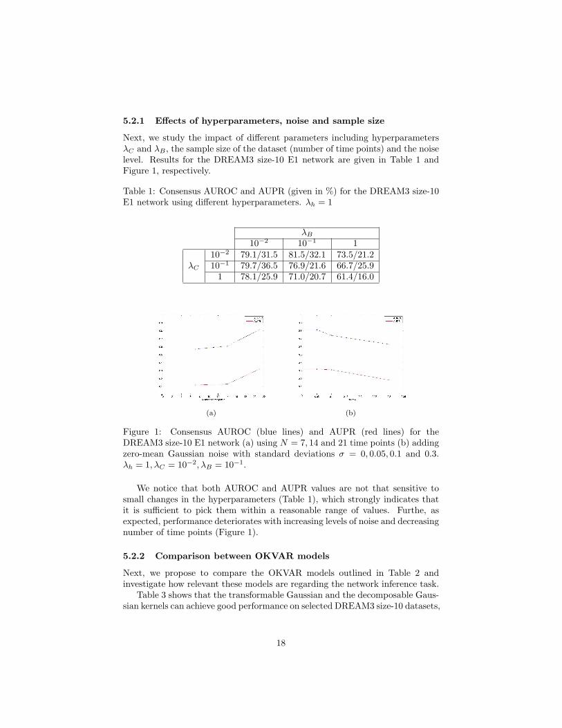
5.2.1 Effects of hyperparameters, noise and sample size

Next, we study the impact of different parameters including hyperparametersλC and λB , the sample size of the dataset (number of time points) and the noiselevel. Results for the DREAM3 size-10 E1 network are given in Table 1 andFigure 1, respectively.

Table 1: Consensus AUROC and AUPR (given in %) for the DREAM3 size-10E1 network using different hyperparameters. λh = 1

λB

10−2 10−1 110−2 79.1/31.5 81.5/32.1 73.5/21.2

λC 10−1 79.7/36.5 76.9/21.6 66.7/25.91 78.1/25.9 71.0/20.7 61.4/16.0

(a) (b)

Figure 1: Consensus AUROC (blue lines) and AUPR (red lines) for theDREAM3 size-10 E1 network (a) using N = 7, 14 and 21 time points (b) addingzero-mean Gaussian noise with standard deviations σ = 0, 0.05, 0.1 and 0.3.λh = 1, λC = 10−2, λB = 10−1.

We notice that both AUROC and AUPR values are not that sensitive tosmall changes in the hyperparameters (Table 1), which strongly indicates thatit is sufficient to pick them within a reasonable range of values. Furthe, asexpected, performance deteriorates with increasing levels of noise and decreasingnumber of time points (Figure 1).

5.2.2 Comparison between OKVAR models

Next, we propose to compare the OKVAR models outlined in Table 2 andinvestigate how relevant these models are regarding the network inference task.

Table 3 shows that the transformable Gaussian and the decomposable Gaus-sian kernels can achieve good performance on selected DREAM3 size-10 datasets,

18

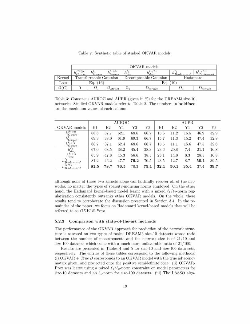
Table 2: Synthetic table of studied OKVAR models.

OKVAR models

hRidgeGauss hℓ1

Gauss hℓ1/ℓ2Gauss hℓ1

dec hℓ1/ℓ2dec hℓ1

Hadamard hℓ1/ℓ2Hadamard

Kernel Transformable Gaussian Decomposable Gaussian HadamardLoss Eq. (16) Eq. (19)Ω(C) 0 Ω1 Ωstruct Ω1 Ωstruct Ω1 Ωstruct

Table 3: Consensus AUROC and AUPR (given in %) for the DREAM3 size-10networks. Studied OKVAR models refer to Table 2. The numbers in boldfaceare the maximum values of each column.

AUROC AUPROKVAR models E1 E2 Y1 Y2 Y3 E1 E2 Y1 Y2 Y3

hRidgeGauss 68.8 37.7 62.1 68.6 66.7 15.6 11.2 15.5 46.9 32.9

hℓ1Gauss 69.3 38.0 61.9 69.3 66.7 15.7 11.3 15.2 47.4 32.8

hℓ1/ℓ2Gauss 68.7 37.1 62.4 68.6 66.7 15.5 11.1 15.6 47.5 32.6

hℓ1dec 67.0 68.5 38.2 45.4 38.3 23.6 20.8 7.4 21.1 16.8

hℓ1/ℓ2dec 65.9 47.8 45.3 56.6 38.5 23.1 14.0 8.3 28.5 16.8

hℓ1Hadamard 81.2 46.2 47.7 76.2 70.5 23.5 12.7 8.7 50.1 39.5

hℓ1/ℓ2Hadamard 81.5 78.7 76.5 70.3 75.1 32.1 50.1 35.4 37.4 39.7

although none of these two kernels alone can faithfully recover all of the net-works, no matter the types of sparsity-inducing norms employed. On the otherhand, the Hadamard kernel-based model learnt with a mixed ℓ1/ℓ2-norm reg-ularization consistently outranks other OKVAR models. On the whole, theseresults tend to corroborate the discussion presented in Section 3.4. In the re-mainder of the paper, we focus on Hadamard kernel-based models that will bereferred to as OKVAR-Prox.

5.2.3 Comparison with state-of-the-art methods

The performance of the OKVAR approach for prediction of the network struc-ture is assessed on two types of tasks: DREAM3 size-10 datasets whose ratiobetween the number of measurements and the network size is of 21/10 andsize-100 datasets which come with a much more unfavorable ratio of 21/100.

Results are presented in Tables 4 and 5 for size-10 and size-100 data sets,respectively. The entries of these tables correspond to the following methods:(i) OKVAR + True B corresponds to an OKVAR model with the true adjacencymatrix given, and projected onto the positive semidefinite cone. (ii) OKVAR-Prox was learnt using a mixed ℓ1/ℓ2-norm constraint on model parameters forsize-10 datasets and an ℓ1-norm for size-100 datasets. (iii) The LASSO algo-

19

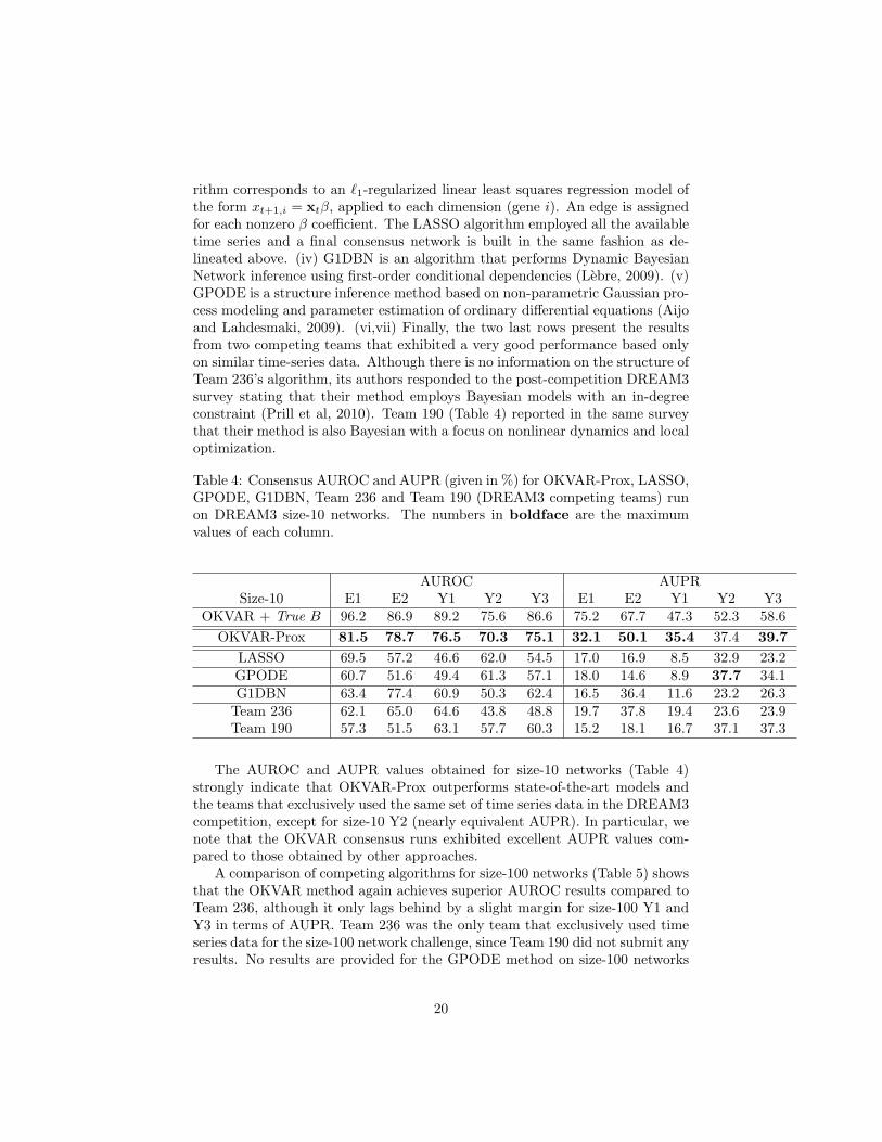
rithm corresponds to an ℓ1-regularized linear least squares regression model ofthe form xt+1,i = xtβ, applied to each dimension (gene i). An edge is assignedfor each nonzero β coefficient. The LASSO algorithm employed all the availabletime series and a final consensus network is built in the same fashion as de-lineated above. (iv) G1DBN is an algorithm that performs Dynamic BayesianNetwork inference using first-order conditional dependencies (Lebre, 2009). (v)GPODE is a structure inference method based on non-parametric Gaussian pro-cess modeling and parameter estimation of ordinary differential equations (Aijoand Lahdesmaki, 2009). (vi,vii) Finally, the two last rows present the resultsfrom two competing teams that exhibited a very good performance based onlyon similar time-series data. Although there is no information on the structure ofTeam 236’s algorithm, its authors responded to the post-competition DREAM3survey stating that their method employs Bayesian models with an in-degreeconstraint (Prill et al, 2010). Team 190 (Table 4) reported in the same surveythat their method is also Bayesian with a focus on nonlinear dynamics and localoptimization.

Table 4: Consensus AUROC and AUPR (given in %) for OKVAR-Prox, LASSO,GPODE, G1DBN, Team 236 and Team 190 (DREAM3 competing teams) runon DREAM3 size-10 networks. The numbers in boldface are the maximumvalues of each column.

AUROC AUPRSize-10 E1 E2 Y1 Y2 Y3 E1 E2 Y1 Y2 Y3

OKVAR + True B 96.2 86.9 89.2 75.6 86.6 75.2 67.7 47.3 52.3 58.6

OKVAR-Prox 81.5 78.7 76.5 70.3 75.1 32.1 50.1 35.4 37.4 39.7

LASSO 69.5 57.2 46.6 62.0 54.5 17.0 16.9 8.5 32.9 23.2GPODE 60.7 51.6 49.4 61.3 57.1 18.0 14.6 8.9 37.7 34.1G1DBN 63.4 77.4 60.9 50.3 62.4 16.5 36.4 11.6 23.2 26.3Team 236 62.1 65.0 64.6 43.8 48.8 19.7 37.8 19.4 23.6 23.9Team 190 57.3 51.5 63.1 57.7 60.3 15.2 18.1 16.7 37.1 37.3

The AUROC and AUPR values obtained for size-10 networks (Table 4)strongly indicate that OKVAR-Prox outperforms state-of-the-art models andthe teams that exclusively used the same set of time series data in the DREAM3competition, except for size-10 Y2 (nearly equivalent AUPR). In particular, wenote that the OKVAR consensus runs exhibited excellent AUPR values com-pared to those obtained by other approaches.

A comparison of competing algorithms for size-100 networks (Table 5) showsthat the OKVAR method again achieves superior AUROC results compared toTeam 236, although it only lags behind by a slight margin for size-100 Y1 andY3 in terms of AUPR. Team 236 was the only team that exclusively used timeseries data for the size-100 network challenge, since Team 190 did not submit anyresults. No results are provided for the GPODE method on size-100 networks

20

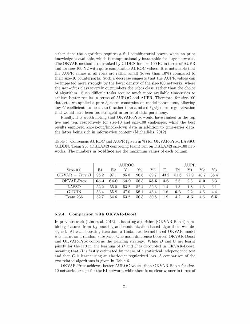
either since the algorithm requires a full combinatorial search when no priorknowledge is available, which is computationally intractable for large networks.The OKVAR method is outranked by G1DBN for size-100 E2 in terms of AUPRand for size-100 Y2 with quite comparable AUROC values. It is noticeable thatthe AUPR values in all rows are rather small (lower than 10%) compared totheir size-10 counterparts. Such a decrease suggests that the AUPR values canbe impacted more strongly by the lower density of the size-100 networks, wherethe non-edges class severely outnumbers the edges class, rather than the choiceof algorithm. Such difficult tasks require much more available time-series toachieve better results in terms of AUROC and AUPR. Therefore, for size-100datasets, we applied a pure ℓ1-norm constraint on model parameters, allowingany C coefficients to be set to 0 rather than a mixed ℓ1/ℓ2-norm regularizationthat would have been too stringent in terms of data parsimony.

Finally, it is worth noting that OKVAR-Prox would have ranked in the topfive and ten, respectively for size-10 and size-100 challenges, while the bestresults employed knock-out/knock-down data in addition to time-series data,the latter being rich in information content (Michailidis, 2012).

Table 5: Consensus AUROC and AUPR (given in %) for OKVAR-Prox, LASSO,G1DBN, Team 236 (DREAM3 competing team) run on DREAM3 size-100 net-works. The numbers in boldface are the maximum values of each column.

AUROC AUPRSize-100 E1 E2 Y1 Y2 Y3 E1 E2 Y1 Y2 Y3

OKVAR + True B 96.2 97.1 95.8 90.6 89.7 43.2 51.6 27.9 40.7 36.4

OKVAR-Prox 65.4 64.0 54.9 56.8 53.5 4.6 2.6 2.3 5.0 6.3

LASSO 52.2 55.0 53.2 52.4 52.3 1.4 1.3 1.8 4.3 6.1G1DBN 53.4 55.8 47.0 58.1 43.4 1.6 6.3 2.2 4.6 4.4Team 236 52.7 54.6 53.2 50.8 50.8 1.9 4.2 3.5 4.6 6.5

5.2.4 Comparison with OKVAR-Boost

In previous work (Lim et al, 2013), a boosting algorithm (OKVAR-Boost) com-bining features from L2-boosting and randomization-based algorithms was de-signed. At each boosting iteration, a Hadamard kernel-based OKVAR modelwas learnt on a random subspace. One main difference between OKVAR-Boostand OKVAR-Prox concerns the learning strategy. While B and C are learntjointly for the latter, the learning of B and C is decoupled in OKVAR-Boost,meaning that B is firstly estimated by means of a statistical independence testand then C is learnt using an elastic-net regularized loss. A comparison of thetwo related algorithms is given in Table 6.

OKVAR-Prox achieves better AUROC values than OKVAR-Boost for size-10 networks, except for the E1 network, while there is no clear winner in terms of

21

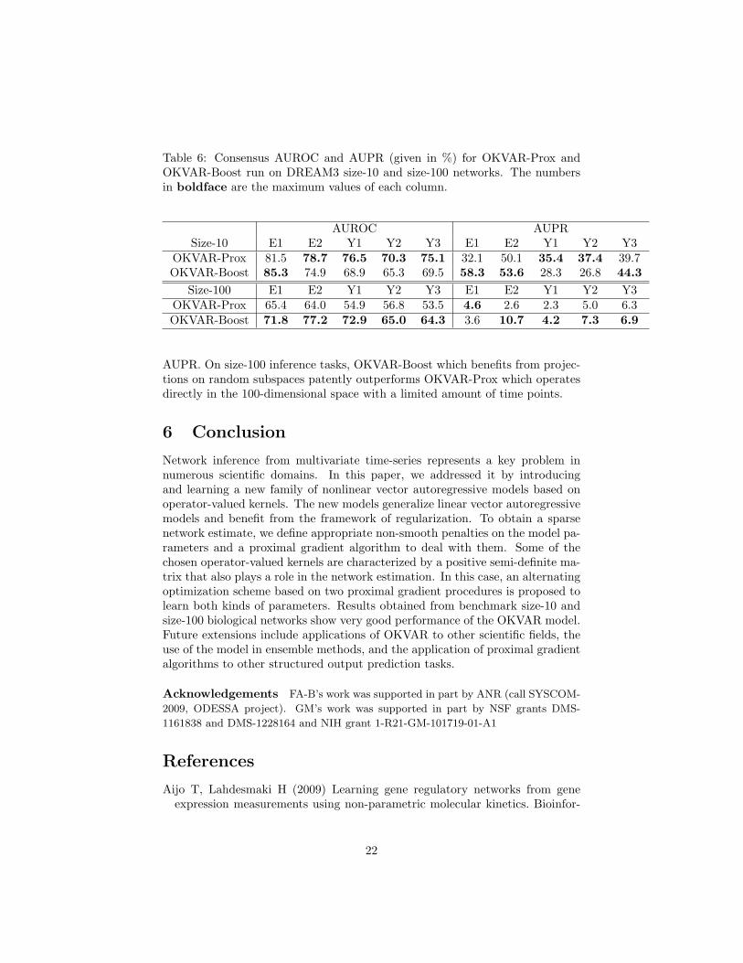
Table 6: Consensus AUROC and AUPR (given in %) for OKVAR-Prox andOKVAR-Boost run on DREAM3 size-10 and size-100 networks. The numbersin boldface are the maximum values of each column.

AUROC AUPRSize-10 E1 E2 Y1 Y2 Y3 E1 E2 Y1 Y2 Y3

OKVAR-Prox 81.5 78.7 76.5 70.3 75.1 32.1 50.1 35.4 37.4 39.7OKVAR-Boost 85.3 74.9 68.9 65.3 69.5 58.3 53.6 28.3 26.8 44.3

Size-100 E1 E2 Y1 Y2 Y3 E1 E2 Y1 Y2 Y3OKVAR-Prox 65.4 64.0 54.9 56.8 53.5 4.6 2.6 2.3 5.0 6.3OKVAR-Boost 71.8 77.2 72.9 65.0 64.3 3.6 10.7 4.2 7.3 6.9

AUPR. On size-100 inference tasks, OKVAR-Boost which benefits from projec-tions on random subspaces patently outperforms OKVAR-Prox which operatesdirectly in the 100-dimensional space with a limited amount of time points.

6 Conclusion

Network inference from multivariate time-series represents a key problem innumerous scientific domains. In this paper, we addressed it by introducingand learning a new family of nonlinear vector autoregressive models based onoperator-valued kernels. The new models generalize linear vector autoregressivemodels and benefit from the framework of regularization. To obtain a sparsenetwork estimate, we define appropriate non-smooth penalties on the model pa-rameters and a proximal gradient algorithm to deal with them. Some of thechosen operator-valued kernels are characterized by a positive semi-definite ma-trix that also plays a role in the network estimation. In this case, an alternatingoptimization scheme based on two proximal gradient procedures is proposed tolearn both kinds of parameters. Results obtained from benchmark size-10 andsize-100 biological networks show very good performance of the OKVAR model.Future extensions include applications of OKVAR to other scientific fields, theuse of the model in ensemble methods, and the application of proximal gradientalgorithms to other structured output prediction tasks.

Acknowledgements FA-B’s work was supported in part by ANR (call SYSCOM-

2009, ODESSA project). GM’s work was supported in part by NSF grants DMS-

1161838 and DMS-1228164 and NIH grant 1-R21-GM-101719-01-A1

References

Aijo T, Lahdesmaki H (2009) Learning gene regulatory networks from geneexpression measurements using non-parametric molecular kinetics. Bioinfor-

22

matics 25:22:2937–2944

Alvarez MA, Rosasco L, D LN (2011) Kernels for vector-valued functions: areview. Tech. rep., MIT CSAIL-TR-2011-033

Auliac C, Frouin V, Gidrol X, d’Alche Buc F (2008) Evolutionary approaches forthe reverse-engineering of gene regulatory networks: a study on a biologicallyrealistic dataset. BMC Bioinformatics 9(1):91

Baldassarre L, Rosasco L, Barla A, Verri A (2010) Vector field learning viaspectral filtering. In: Balczar J, Bonchi F, Gionis A, Sebag M (eds) MachineLearning and Knowledge Discovery in Databases, Lecture Notes in ComputerScience, vol 6321, Springer Berlin / Heidelberg, pp 56–71

Beck A, Teboulle M (2010) Gradient-based algorithms with applications to sig-nal recovery problems. In: Palomar D, Eldar Y (eds) Convex Optimizationin Signal Processing and Communications, Cambridge press, pp 42–88

Bolstad A, Van Veen B, Nowak R (2011) Causal network inference via groupsparsity regularization. IEEE Trans Signal Process 59(6):2628–2641

Brouard C, d’Alche Buc F, Szafranski M (2011) Semi-supervised penalized out-put kernel regression for link prediction. In: ICML-2011, pp 593–600

Buhlmann P, van de Geer S (2011) Statistics for High-Dimensional Data: Meth-ods, Theory and Applications. Springer

Caponnetto A, CA, Pontil M, Ying Y (2008) Universal multitask kernels. JMach Learn Res 9

Chatterjee S, Steinhaeuser K, Banerjee A, Chatterjee S, Ganguly AR (2012)Sparse group lasso: Consistency and climate applications. In: SDM, SIAM /Omnipress, pp 47–58

Chou I, Voit EO (2009) Recent developments in parameter estimation andstructure identification of biochemical and genomic systems. Math Biosci219(2):57–83

Dinuzzo F, Fukumizu K (2011) Learning low-rank output kernels. In: Proceed-ings of the 3rd Asian Conference on Machine Learning, JMLR: Workshop andConference Proceedings, vol 20

Dondelinger F, Lebre S, Husmeier D (2013) Non-homogeneous dynamic bayesiannetworks with bayesian regularization for inferring gene regulatory networkswith gradually time-varying structure. Machine Learning Journal 90(2):191–230

Friedman N (2004) Inferring cellular networks using probabilistic graphical mod-els. Science 303(5659):799–805

23

Gilchrist S, Yankov V, Zakrajsek E (2009) Credit market shocks and economicfluctuations: Evidence from corporate bond and stock markets. Journal ofMonetary Economics 56(4):471–493

Hartemink A (2005) Reverse engineering gene regulatory networks. Nat Biotech-nol 23(5):554–555

Iba H (2008) Inference of differential equation models by genetic programming.Inf Sci 178(23):4453–4468

Kadri H, Rabaoui A, Preux P, Duflos E, Rakotomamonjy A (2011) Functionalregularized least squares classication with operator-valued kernels. In: ICML-2011, pp 993–1000

Kolaczyk ED (2009) Statistical Analysis of Network Data: Methods and Models.Springer: series in Statistics

Kramer MA, Eden UT, Cash SS, Kolaczyk ED (2009) Network inference withconfidence from multivariate time series. Physical Review E 79(6):061,916+

Lawrence N, Girolami M, Rattray M, Sanguinetti G (eds) (2010) Learning andInference in Computational Systems Biology. MIT Press

Lebre S (2009) Inferring dynamic genetic networks with low order independen-cies. Statistical applications in genetics and molecular biology 8(1):1–38

Lim N, Senbabaoglu Y, Michailidis G, d’Alche Buc F (2013) Okvar-boost: anovel boosting algorithm to infer nonlinear dynamics and interactions in generegulatory networks. Bioinformatics 29(11):1416–1423

Liu Y, Niculescu-Mizil A, Lozano A (2010) Learning temporal causal graphs forrelational time-series analysis. In: Furnkranz J, Joachims T (eds) ICML-2010

Maathuis M, Colombo D, Kalish M, Buhlmann P (2010) Predicting causal effectsin large-scale systems from observational data. Nature Methods 7:247–248

Margolin I Aand Nemenman, Basso K, Wiggins C, Stolovitzky G, Favera R, Cal-ifano A (2006) Aracne: an algorithm for the reconstruction of gene regulatorynetworks in a mammalian cellular context. BMC Bioinf 7(Suppl 1):S7

Mazur J, Ritter D, Reinelt G, Kaderali L (2009) Reconstructing nonlinear dy-namic models of gene regulation using stochastic sampling. BMC Bioinfor-matics 10(1):448

Meinshausen N, Buhlmann P (2006) High dimensional graphs and variable se-lection with the lasso. Annals of Statistics 34:1436–1462

Micchelli CA, Pontil MA (2005) On learning vector-valued functions. NeuralComputation 17:177–204

24

Michailidis G (2012) Statistical challenges in biological networks. Journal ofComputational and Graphical Statistics 21(4):840–855

Michailidis G, d’Alche Buc F (2013) Autoregressive models for gene regula-tory network inference: Sparsity, stability and causality issues. Math Biosci246(2):326 – 334

Morton R, Williams KC (2010) Experimental Political Science and the Studyof Causality. Cambridge University Press

Murphy KP (1998) Dynamic bayesian networks: representation, inference andlearning. PhD thesis, Computer Science, University of Berkeley, CA, USA

Parry M, Canziani O, Palutikof J, van der Linden P, Hanson C, et al (2007) Cli-mate change 2007: impacts, adaptation and vulnerability. IntergovernmentalPanel on Climate Change

Perrin BE, Ralaivola L, A M, S B, Mallet J, d’Alche Buc F (2003) Gene networksinference using dynamic bayesian networks. Bioinformatics 19(S2):38–48

Prill R, Marbach D, Saez-Rodriguez J, Sorger P, Alexopoulos L, Xue X, ClarkeN, Altan-Bonnet G, Stolovitzky G (2010) Towards a rigorous assessment ofsystems biology models: The dream3 challenges. PLoS ONE 5(2):e9202

Raguet H, Fadili J, Peyre G (2011) Generalized forward-backward splitting.arXiv preprint arXiv:11084404

Richard E, Savalle PA, Vayatis N (2012) Estimation of simultaneously sparseand low rank matrices. In: Langford J, Pineau J (eds) ICML-2012, Omnipress,New York, NY, USA, pp 1351–1358

Senkene E, Tempel’man A (1973) Hilbert spaces of operator-valued functions.Lithuanian Mathematical Journal 13(4)

Shojaie A, Michailidis G (2010) Discovering graphical granger causality using atruncating lasso penalty. Bioinformatics 26(18):i517–i523

Yuan M, Lin Y (2006) Model selection and estimation in regression with groupedvariables. Journal of the Royal Statistical Society: Series B 68(1):49–67

Zou C, Feng J (2009) Granger causality vs. dynamic bayesian network inference:a comparative study. BMC Bioinformatics 10(1):122

25