Vector Autoregressive moving average identification for
44
Econometrics & Business Statistics Version of March 22, 2011 Vector Autoregresive Moving Average Identification for Macroeconomic Modeling: A New Methodology D. S. Poskitt ∗ Department of Econometrics & Business Statistics, Monash University Abstract This paper develops a new methodology for identifying the structure of VARMA time se- ries models. The analysis proceeds by examining the echelon canonical form and presents a fully automatic data driven approach to model specification using a new technique to determine the Kronecker invariants. A novel feature of the inferential procedures devel- oped here is that they work in terms of a canonical scalar ARMAX representation in which the exogenous regressors are given by predetermined contemporaneous and lagged values of other variables in the VARMA system. This feature facilitates the construction of algorithms which, from the perspective of macroeconomic modeling, are efficacious in that they do not use AR approximations at any stage. Algorithms that are applicable to both asymptotically stationary and unit-root, partially nonstationary (cointegrated) time series models are presented. A sequence of lemmas and theorems show that the algorithms are based on calculations that yield strongly consistent estimates. The infer- ential potential of the techniques are illustrated using an example drawn from the real business cycle literature. * Corresponding address: Don Poskitt, Department of Econometrics and Business Statistics, Monash Uni- versity, Victoria 3800, Australia Tel.:+61-3-9905-9378; fax:+61-3-9905-5474. E-mail address: [email protected]
Transcript of Vector Autoregressive moving average identification for
Econometrics & Business Statistics Version of March 22, 2011
Vector Autoregresive Moving Average Identification forMacroeconomic Modeling: A New Methodology
D. S. Poskitt∗
Department of Econometrics & Business Statistics, Monash University
Abstract
This paper develops a new methodology for identifying the structure of VARMA time se-
ries models. The analysis proceeds by examining the echelon canonical form and presents
a fully automatic data driven approach to model specification using a new technique to
determine the Kronecker invariants. A novel feature of the inferential procedures devel-
oped here is that they work in terms of a canonical scalar ARMAX representation in
which the exogenous regressors are given by predetermined contemporaneous and lagged
values of other variables in the VARMA system. This feature facilitates the construction
of algorithms which, from the perspective of macroeconomic modeling, are efficacious in
that they do not use AR approximations at any stage. Algorithms that are applicable
to both asymptotically stationary and unit-root, partially nonstationary (cointegrated)
time series models are presented. A sequence of lemmas and theorems show that the
algorithms are based on calculations that yield strongly consistent estimates. The infer-
ential potential of the techniques are illustrated using an example drawn from the real
business cycle literature.
∗Corresponding address: Don Poskitt, Department of Econometrics and Business Statistics, Monash Uni-versity, Victoria 3800, Australia Tel.:+61-3-9905-9378; fax:+61-3-9905-5474.
E-mail address: [email protected]
VARMA Models in Macroeconomics 1
1 Introduction
Since the appearance of the seminal work of Sims (1980) on the relationship between abstract
macroeconomic variables and stylized facts as represented by statistical time series models,
vector autoregressive (VAR) models of the form
A(B)yt = ut, t = 1, . . . , T, (1.1)
have become the cornerstone of much macroeconomic modeling. In equation (1.1) the vector
yt = (y1t, . . . , yvt)′ denotes a v component observable process. The v × v matrix operator
A(z) = A0 +A1z1 + · · · +Apz
p in the backward shift or lag operator B, viz. Byt = yt−1,
determines the basic evolutionary properties of the observed process yt and the stochastic
disturbance, ut = (u1t, . . . , uvt)′, which is unobserved, determines how chance or random
influences enter the system.
Apart from their use as the main tool in numerous multivariate macroeconomic forecast-
ing applications (as in Doan, Litterman and Sims, 1984), VARs have found broad applica-
tion as the foundation of much dynamic macroeconomic modeling. They are used to study
long-run equilibrium behaviour, with researchers investigating vector error correction models
constructed from VARs fitted to macroeconomic time series (following Engle and Granger,
1987). In structural VAR (SVAR) models, VARs coupled with restrictions derived from
economic theory are used to examine the effects of structural shocks on key macroeconomic
variables (see Christiano, Eichenbaum and Vigfusson, 2006, for a recent contribution). In
dynamic stochastic general equilibrium (DSGE) models, VARs are used as auxiliary models
for indirect estimation of the DSGE model parameters (Smith, 1993), and to provide ap-
proximations to the solutions of DSGE models that have been expanded around their steady
state (Del Negro and Schrfheide, 2004).
This ubiquitous use of VARs has occurred despite their limitations being well known.
First, VAR specifications form an unattractive class of models for modeling macroeconomic
variables since they are not closed under aggregation, marginalization or the presence of
measurement error, see Fry and Pagan (2005) and Lutkepohl (2005). Secondly, economic
models often imply that the observed processes have a vector autoregressive moving aver-
age (VARMA) representation with a non-trivial moving average component, as in Cooley
and Dwyer (1998), and, more recently, Fernandez-Villaverde, Rubio-Ramırez, Sargent and
Watson (2007).
In order to expand the representation in (1.1) into the more general VARMA class, let
us assume that ut is a full rank, zero mean, p-dependent stationary process with covariance
E[utu′t+τ ] = Γξ(τ) = Γξ(−τ)′, τ = 0,±1,±2, . . . , p. This implies the existence of a sequence
of zero mean, uncorrelated random variables εt, defined on the same probability space as ut,
such that ut = M(B)εt, t = 1, . . . , T, where E[εtε′t] = Σ > 0 and, without loss of generality,
the v× v matrix operator M(z) = M0 +M1z1 + · · ·+Mpz
p satisfies det(M(z)) = 0, |z| < 1
(see Hannan, 1971, Theorem 10’ and the associated discussion). Substituting ut = M(B)εt
VARMA Models in Macroeconomics 2
into equation (1.1) gives us the VARMA form
A(B)yt = M(B)εt. (1.2)
The process yt is assumed to evolve over the time period t = 1, . . . , T , according to the
specification given in (1.2), starting from initial values given by yt = εt = 0, t ≤ 0. The
stochastic behaviour of yt is now clearly dependent on the operator pair [A(z) : M(z)], with
random variation induced by the random disturbances, or shocks, εt. More formally, it will
be assumed that the disturbances, or innovations, possess the following probability structure:
Assumption 1 The process εt =(ε1t, . . . , εvt
)′is a stationary, ergodic, martingale differ-
ence sequence. Thus if Ft denotes the σ-algebra generated by ε(s), s ≤ t, then E[εt | Ft−1] =
0. Furthermore, E[εtε′t | Ft−1] = Σ > 0 and E[εkjt] < ∞, j = 1, . . . , v, k ≥ 2.
In situations where the theoretical background gives rise to a VARMA model it might be
expected that a VAR of high order could be used to approximate the true VARMA structure.
Results in the recent literature suggest, however, that such an approach could be fraught
with difficulties. Conditions under which the economic shocks and impulse responses from
an economic model are matched by those of a (S)VAR are examined in Fernandez-Villaverde
et al. (2007), and Chari, Kehoe and McGrattan (2007) conclude from their analysis that the
currently available data is prohibitive, leading to VARs that have too short a lag length and
that provide poor approximations and unreliable inferences. For a simulated model that has
both DSGE elements and data dynamics Kapetanios, Pagan and Scott (2007) suggest that
a sample of 30000 observations with a VAR of order 50 is required to adequately capture the
effect of some of the structural shocks. Ravenna (2007) also points out that using a VAR
to characterize the dynamics of a model that in truth leads to a VARMA structure can be
misleading, and warns researchers to be cautious when relying on evidence from VARs to
build such models.
Given that the limitations and pitfalls of VARs for macroeconomic analysis have been
well documented, one might imagine that applied macroeconomic researchers would have
been compelled to consider implementing VARMA models instead. Practitioners appear to
have been reluctant to embrace VARMA models however. The reason for this reluctance is,
perhaps, that the complexities associated with the identification and estimation of VARMA
models stand in sharp contrast to the ease and accessibility of VARs.
Multivariate time series models have, of course, been given considerable attention in the
past and accounts of many of the methods and techniques available are given in Hannan
and Deistler (1988) and Lutkepohl (2005), for example. Nevertheless, the question of how
best to determine the internal structure of a VARMA model in a direct and straightforward
manner has not been completely resolved. Two techniques of identification predominate:
1. The scalar-component methodology pioneered by Tiao and Tsay (1989), and further
developed in Athanasopoulos and Vahid (2008). This method uses an adaptation
of the canonical correlation analysis introduced in Akaike (1974b) to detect various
linear dependencies implied by different structures. It relies on the solution of different
VARMA Models in Macroeconomics 3
eigenvalue problems and solves the underlying multiple decision problem via a sequence
of hypothesis tests;
2. The echelon form methodology developed in Hannan and Kavalieris (1984) and Poskitt
(1992). In this approach the coefficients of an VARMA model expressed in echelon
canonical form are estimated and the associated Kronecker indices determined using
regression techniques and model selection criteria, a la AIC (Akaike, 1974a), BIC
(Schwarz, 1978) or HQ (Hannan and Quin, 1979).
An illuminating exposition of the similarities and differences between scalar-component mod-
els and echelon forms is given in Tsay (1991), and Athanasopoulos, Poskitt and Vahid (2010)
present a detailed analysis and comparison of these two techniques, highlighting the relative
merits and advantages of each method (c.f. Nsiri and Roy, 1992). The lack of a single well-
defined multivariate parallel to the classical Box-Jenkins ARMA methodology for univariate
time series has, no doubt, discouraged researchers from employing VARMAs in practice, de-
spite the fact that “While VARMA models involve additional estimation and identification
issues, these complications do not justify systematically ignoring these moving average com-
ponents, – – – – –.” (Cooley and Dwyer, 1998). The broad aim of this paper is to fill this
gap and operationalize the use of VARMA models to the point where they can be routinely
employed as part of the basic toolkit of the applied macroeconomist.
The paper develops a coherent methodology for identifying and estimating VARMA
models that can be fully automated. The approach adopted is to construct a modification of
the echelon form methodology using a new technique to determine the Kronecker invariants.
The scalar-components method is not considered here, firstly, because it is not amenable to
automation in a manor similar to that used for VARs as is the echelon form methodology.
Secondly, given the significance of cointegration in the practical analysis of economic and
financial time series we wish to investigate unit-root nonstationary cointegrated systems
and examine the consequences of applying our methods to identify cointegrated VARMA
structures. Extensions of the echelon form methodology to cointegrated VARMA models
have been analysised in Lutkepohl and Claessen (1997), Bartel and Lutkepohl (1998) and
Poskitt (2003, 2006) (See also Lutkepohl, 2005, Chapter 14.), but to our knowledge similar
extensions of the scalar-components methodology to cointegrated processes are not currently
available.
In both the scalar-components and the echelon form methodologies the initial step is to
fit a high-order VAR, the associated residuals are then used as plug in estimates for the
unknown innovations in subsequent stages of the analysis. The applied macroeconomic lit-
erature referred to earlier questions the practical efficacy of using long VAR approximations,
however, and intimates that the quality of the VAR innovations estimates is likely to be
poor. Moreover, Poskitt (2005) presents theoretical arguments showing why the use of the
first stage VAR residuals can lead to serious overestimation of the VARMA orders. A novel
feature of the inferential procedure developed here is that it does not require the use of
autoregressive approximations, thereby circumventing any problems that might be inherent
in using a VAR in a macroeconomic modeling context.
VARMA Models in Macroeconomics 4
The paper is organised as follows. The following section defines the the inverse echelon
form and Kronecker invariants. Section 3 analyzes a single equation canonical representation
that forms the basis of the identification of the Kronecker invariants. An Algorithm for the
identification of the Kronecker invariants of a stationary ARMA process is then presented
in Section 4. Section 5 gives theoretical results stating conditions under which almost sure
convergence of the estimated values to the true Kronecker invariants can be achieved. Section
6 shows how the canonical representation considered in Section 3 can be adapted to allow
for cointegrated processes and Section 7 then presents a modification of the identification
procedure that gives rise to a strongly consistent model selection process that is applicable
to cointegrated processes. The eighth section of the paper presents the theoretical results
underpinning the technique outlined in Section 7. Section 9 presents a brief conclusion and
illustrates the underlying ideas and results discussed in the paper by examining the impulse
responses derived from a real business cycle model.
2 The Inverse Echelon Form and Kronecker Invariants
Before continuing let us establish some additional notational conventions and assumptions.
The order of [A(z) : M(z)] is defined as p = max1≤i≤v ni where, for i = 1, . . . , v, ni =
δi [A(z) : M(z)] denotes the polynomial degree of the ith row of [A(z) : M(z)]. The integers
nr, r = 1, . . . , v, are called the Kronecker indices. The Kronecker indices determine the lag
structure of the, so called, inverse echelon form, which is characterized by an operator pair
[A(z) : M(z)] with polynomial elements that satisfy for all r, c = 1, . . . , v ,
(i) arc,0 = mrc,0 ,
(ii) mrr(z) = 1 +mrr,1z + . . .+mrr,nrznr ,
mrc(z) = mrc,nr−nrc+1znr−nrc+1 + . . .+mrc,nrz
nr and
(iii) arc(z) = arc,0 + arc,1z + . . .+ arc,nrznr , (2.1)
where
nrc =
{min(nr + 1, nc) r ≥ c ,
min(nr, nc) r < c .
The restrictions implicit in (2.1) differ from those commonly found in the literature on
echelon forms, see Hannan and Deistler (1988, §2.5) for detailed a discussion of the conven-
tional case and Lutkepohl (2005, §14.2.2) for the structure in (2.1). Conditions (2.1)(i)&(ii)
imply that the standard normalization A0 = M0, with unit leading diagonal, is imposed, but
(2.1)(ii) implies that additional exclusion constraints are placed upon lower order coefficients
of M(z) according to the relative lag lengths, rather than A(z). The latter feature arises
because the inverse echelon form is constructed from the mapping [A(z) : M(z)] 7→ Ψ(z)
defined by M(z)Ψ(z) = A(z), wherein the coefficients Ψ0,Ψ1,Ψ2, . . . are derived from the
VARMA Models in Macroeconomics 5
recursive relationships
i∑j=0
MjΨi−j = Ai, i = 0, . . . , p, and
p∑j=0
MjΨi−j = 0, i = p+ 1, . . . . (2.2)
Note that Ψ0 = I and ∥Ψi∥ < ∞, i = 0, 1, . . ., where ∥Ψj∥2 = trΨjΨ′j , the Euclidean norm.
If detM(z) = 0, |z| ≤ 1 then ∥Ψi∥ → 0 at an exponential rate as i → ∞ and the power
series Ψ(z) = limN→∞∑N
0 Ψizi will be convergent for |z| ≤ 1. The nomenclature is based
on the fact that it is the mapping obtained via (2.2) which allows us to invert the VARMA
representation and express the innovation process in terms of the model parameters and the
observables, namely εt =∑t−1
j=0Ψjyt−j . If we let ARMAE(ν) denote the class of all VARMA
models in inverse echelon form with multi-index ν = {n1, . . . , nv}, then ARMAE(ν) defines
a canonical structure for the set of VARMA models with McMillan degree m =∑v
i=1 ni.
Assumption 2 The pair [A(z) : M(z)] are (left) coprime and [A(z) : M(z)] ∈ ARMAE(ν).
It will be supposed that neither detA(z) or detM(z) is identically zero and that the de-
terminants of the polynomial matrices A(z) and M(z) satisfy detA(z) = 0 |z| < 1 and
detM(z) = 0, |z| ≤ 1.
Note that Assumption 2 allows for the possibility that A(z) has zeroes on the unit circle.
Let us assume that detA(z) has ζ ≤ v roots of unity, all other zeroes lie outside the unit
circle, and that the individual series yit, i = 1, . . . , v, are asymptotically stationary after first
differencing, i.e., △yt = (1 − B)yt = yt − yt−1, t = 1, . . . , T , is asymptotically stationary.
Then the process yt is non-stationary and cointegrated. We will deal with cointegrated
processes in detail below, having first examined the asymptotically stationary case. For
the stationary case the condition on the zeroes of A(z) in Assumption 2 is strengthened
to detA(z) = 0, |z| ≤ 1. We will refer to the strengthened version of Assumption 2 as
Assumption 2′.
The Kronecker indices are not invariant with respect to an arbitrary reordering of the
elements of yt and to this extent the inverse echelon canonical form is only unique mod-
ulo such rotations. The variables in yt = (y1t, . . . , yvt)′ can be permuted, however, such
that the Kronecker indices of (yr(1)t, . . . , yr(v)t)′ are arranged in descending order, nr(1) ≥
nr(2) ≥ · · · ≥ nr(v), where r(j), j = 1, . . . , v, denotes a permutation of 1, . . . , v that induces
the ordering. The r(j), j = 1, . . . , v, are unique modulo rotations that leave the ordering
nr(1) ≥ · · · ≥ nr(v) unchanged and (r(j), nr(j)), j = 1, . . . , v, are referred to as the Kronecker
invariants. When expressed in terms of the Kronecker invariants not only is the representa-
tion of the system in inverse echelon form canonical but the coefficient matrix A0 = M0 is
lower triangular and the individual variables yr(j)t, j = 1, . . . , v are uniquely characterized.
In practice, of course, the Kronecker invariants will not be known and we wish to consider
identifying them in the sense of estimating or determining them from the data. Moreover,
given that the numbering of the variables in yt assigned by the practitioner is arbitrary,
VARMA Models in Macroeconomics 6
identification of the Kronecker invariants involves the determination of not only the values of
nr(1) ≥ nr(2) ≥ · · · ≥ nr(v), but also the permutation (r(1), . . . , r(v))′ of the labels (1, . . . , v)′
attached to the variables. At the risk of getting ahead of ourselves, suppose that we know
that max{n1, . . . , nv} ≤ h. We might contemplate examining all ARMA structures in the
set {ARMAE(ν) : ν ∈ {ν = (n1, . . . , nv) : 0 ≤ nr ≤ h, r = 1, . . . , v}}. If a full search over
all such structures were to be conducted then a total of (h+1)v specifications would have to
be examined; if v = 5 and h = 12, say, this means estimating 371293 different ARMAE(ν)
models. This brings us face to face with the curse of dimensionality.
Considerable savings can be made, however, if the pairs (r(j), nr(j)) associated with
yr(j)t, j = 1, . . . , v, can be identified on a variable by variable, or equivalently, equation
by equation, basis. Identification of the Kronecker invariants equation by equation involves
examining v(h + 1) different specifications at most; if v = 5 and h = 12 this gives an
upper bound of 65, rather than the previous total of 371293. To determine the Kronecker
invariants variable by variable, however, we need to construct from the ARMAE(ν) system
representation a univariate specification for yr(j)t that allows the Kronecker invariant pairs
(r(j), nr(j)), j = 1, . . . , v, to be appropriately isolated. We derive such a specification in the
next section.
3 A Single Equation Canonical Structure
Various aspects of the relationship between VARMA models and the structure of the indi-
vidual univariate series have been discussed in the literature, but none consider specifications
that are suitable for our current purposes since they all convolve the individual operators in
such a way as to disguise their underlying polynomial degrees. The final form (Wallis, 1977),
for example, is obtained by pre-multiplying (1.2) by the adjoint of A(z), denoted adjA(z),
to give
detA(B)yt = adjA(B)M(B)εt . (3.1)
In general, the operators on the left and right hand sides of this expression all have degree
equal to m. Consequently, although (3.1) can be used to determine the McMillan degree of
the overall system (see Remark 3 below), it does not yield univariate specifications suitable
for the identification of the Kronecker invariants.
In order to identify nr(1) ≥ nr(2) ≥ · · · ≥ nr(v), we now introduce a single equation
canonical structure, derived from (1.2), that does not obscure the Kronecker invariants. The
single equation form depends upon the following lemma.
Lemma 3.1 Suppose that yt is an ARMA process as in (1.2) satisfying Assumptions 1 and
2. Then for each choice of the process νt = ujt, j = 1, . . . , v, where
ut =
u1t...
uvt
= A(B)yt ,
there exists a zero mean, scalar white noise process ηt, with variance σ2η, defined on the same
VARMA Models in Macroeconomics 7
probability space as yt, such that
νt = ηt + µ1ηt−1 + . . .+ µnηt−n,
where n = nj and the coefficients µ1, . . . , µn of µ(z) − 1 =∑n
s=1 µszs are such that the
auto-covariance generating function of νt equals σ2ηµ(z)µ(z
−1) and µ(z) = 0, |z| ≤ 1.
A consequence of Lemma 3.1 is that each variable in yt admits a scalar ARMAX rep-
resentation in which the exogenous variables are chosen from contemporaneous and lagged
values of other variables in the VARMA system.
Proposition 3.1 Let yt be an ARMA process satisfying Assumptions 1 and 2 , and suppose
that the variables have been ordered (renumbered) according to the Kronecker invariants, so
that, with a slight abuse of notation, yt = (y1t, . . . , yvt)′ = (yr(1)t, . . . , yr(v)t)
′ and nj = nr(j),
j = 1, . . . , v. Then for each j = 1, . . . , v the jth equation in (1.2) is equivalent to a scalar
ARMAX specification for zt = yjt of the form
zt +
n∑s=1
αszt−s +
j−1∑i=1
βiyit +
v∑i=1i =j
n∑s=1
βi,syit−s = ηt +
n∑s=1
µsηt−s , (3.2)
where the order n = nj. Moreover, α(z) = 1+∑n
s=1 αszs, β(z) = (β1+
∑ns=1 β1,sz
s, . . . , βj−1+∑ns=1 βj−1,sz
s, 0,∑n
s=1 βj+1,szs, . . . ,
∑ns=1 βv,sz
s) and µ(z) = 1+∑n
s=1 µszs are coprime, and
the regressors yit, i = 1, . . . , j − 1, and yit−s, i = 1, . . . , v, i = j, s = 1, . . . , n are predeter-
mined relative to zt in the representation (3.2).
Two aspects of Proposition 3.1 that are of particular interest here are; (i) that the degree
of the lag operators in (3.2) depends only on the value of the Kronecker invariant associated
with the variable at hand, and (ii) that the contemporaneous component depends only on
those variables associated with a smaller Kronecker invariant. This means that knowledge of
the Kronecker index associated with yr(j)t tells us the lag length of all the variables appearing
in the ARMAX realization of yr(j)t, and knowing the ranking of the Kronecker index relative
to the other indices, i.e. knowledge that nr(j) ≥ nr(i), i = j + 1, . . . , v, tells us about
the recursive structure. Note that explicit knowledge of the values of the other Kronecker
invariants is not required, the ARMAX specification of the r(j)th equation being a known
function of dj(n) = (j − 1) + (v + 1)n parameters. These features suggest that a sensible
approach to adopt to the identification of the Kronecker invariants is to search through a
collection of ARMAX models for each variable supposing that the fitted order coincides with
the smallest unknown Kronecker invariant. The details of such a procedure are presented in
the following section.
4 Identification Algorithm: Stationary Case
Let yt, t = 1, . . . , T denote a realisation of T observations where yt is an ARMA process as
in (1.2) satisfying Assumptions 1 and 2′. We have already observed that identification of the
Kronecker invariants involves the determination of both the values of nr(1) ≥ · · · ≥ nr(v) and
VARMA Models in Macroeconomics 8
the permutation of the variables in yt, P(1, . . . , v)′ = (r(1), . . . , r(v))′ say, that results in an
ARMAE form with multi-index (nr(1), . . . , nr(v)) for Pyt = (yr(1)t, . . . , yr(v)t)′. The following
algorithm identifies the Kronecker invariants equation by equation whilst constructing P
via a sequence of elementary row operations. The algorithm exploits the implications of
Proposition 3.1 and represents an adaptation to VARMA models of an approach to the
identification of the order of scalar processes first outlined in Poskitt and Chung (1996).
ALGORITHM–ARMAE(ν).
Initialization: Set n = 1, j = v, P = I and N = {1, . . . , v}. Compute the mean corrected
values yt = yt − y, t = 1, . . . , T , where y = T−1∑T
i=1 yt. For each i ∈ N , set σ2η,i(0)
equal to the residual mean square from the regression of yit on ykt, k = 1, . . . , v, k = i.
while: j ≥ 1
for i(k) ∈ N , k = 1, . . . , v,
1. Set yt = Ei(k),j [Pyt], where Er1,r2 denotes the v × v elementary matrix that
induces an interchange of rows r1 and r2 in H when postmultiplied by H,
and evaluate initial estimates of the jth scalar ARMAX form for zt = yi(k)t:
(a) Construct estimates of the nonzero coefficients in a(z) = e′jA(z), the jth
row of A(z) = Ei(k),jPA(z)P′E′i(k),j , by solving the equations
n∑s=0
asCy(r + s) = 0, r = n+ 1, . . . , 2n, (4.1)
for a0 = (a1,0, . . . , a(j−1),0, 1, 0, . . . , 0), and as = (a1,s, . . . , av,s), s =
1, . . . , n, where
Cy(r) = Cy(−r)′ = T−1
T−|r|∑t=1
yty′t−r
for r = 1, · · · , T − 1. Now set αs = aj,s, s = 1, . . . , n,βi = ai,0, i =
1, . . . , j − 1, andβi,s =
ai,s, i = 1, . . . , v, i = j, s = 1, . . . , n.
(b) For r = 1, · · · , n form
Cv(r) = Cv(−r) =
n∑s=0
n∑u=0
asCy(r + s− u)au=
∫ π
−π
a(ω)Iy(ω)a(ω)∗ exp(−ıωr)dω (4.2)
where a(ω) = a0 + a1 exp(ıω) + · · ·+ an exp(ıωn) = a(z)∣∣z=eıω
and
Iy(ω) =1
2π
T−1∑s=−T+1
Cy(s) exp(ıω) .
Set Sv(ω) =
1
2π
n∑s=−n
Cv(s) exp(ıωs) . (4.3)
VARMA Models in Macroeconomics 9
Compute estimates µs, s = 1, . . . , n, of the coefficients in the scalar
moving average representation of vt = ujt, where ujt = e′jM(B)εt and
M(z) = Ei(k),jPM(z), by solving the equation system
n∑s=0
µsCiv(l + s) = 0, l = 1, . . . , n
where
Civ(r) =
∫ π
−π
a(ω)Iy(ω)a(ω)∗Sv(ω)2
exp(−ıωr)dω . (4.4)
2. Compute a pseudo maximum likelihood estimate (pseudo MLE) of the inno-
vation variance σ2η.
(a) Form the v + 1 vector sequence (ξ′t,φt, )
′ by solving[ ξtφt
]+
n∑s=1
µs
[ ξt−sφt−s
]=
[ytηt]
for t = 1, . . . , T where
ηt =
n∑s=0
aj,sy(t− s)−n∑
s=1
µsηt−s
=
n∑s=0
αszt−s +
j−1∑i=1
βiyit +
v∑i=1i =j
n∑s=1
βi,syit−s −
n∑s=1
µsηt−s
and the recursions are initiated at ηt = 0 and (ξ′t,φt, )
′ = 0′, t ≤ 0.
(b) Set cη(0) = T−1∑T
tη2t and calculate
cηξ(s) = T−1
T∑t=s+1
ηtξ′t−s and cηφ(s) = T−1T∑
t=s+1
ηt φt−s .
Now compute the mean squared error
σ2
η(n) = cη(0) +
n∑s=0
∆ascηξ(s)′ − n∑s=1
∆µscηφ(s)
where ∆as, s = 0, . . . , n, and ∆µs, s = 1, . . . , n, denote the coefficient
values obtained from the Toeplitz regression of ηt on −ξit, i = 1, . . . , j−1,
and −ξt−s, s = 1, . . . , n, and φt−s, s = 1, . . . , n.
3. Apply model selection rule:
(a) Evaluate the criterion function
ICT (n) = T log σ2
η(n) + pT (dj(n))
where the penalty term pT (dj(n)) > 0 is a real valued function, mono-
tonically increasing in dj(n) and non-decreasing in T .
VARMA Models in Macroeconomics 10
(b) if ICT (n) > ICT (n− 1);
set r(j) = i(k); nr(j) = n− 1; and
update P = Ei(k),jP; N = N \ i(k); j = j − 1.
end
end for i(k) ∋ N .
if n < hT ;
increment n = n+ 1.
else
for i(k) ∈ N , k = 1, . . . , v,
set nr(j) = n; r(j) = i(k); and
update P = Ei(k),jP; N = N \ i(k); j = j − 1.
end for i(k) ∋ N .
end
end when j = 0.
Some remarks on the algorithm’s rationale and numerical implementation are in order:
REMARK 1. The first step of the algorithm is designed to provide first stage consistent
estimates of the parameters in the scalar ARMAX representation in (3.2). Step 1(a) is based
on the fact that from Proposition 3.1 it follows that yt−n−s, s = 1, . . . , n, are orthogonal to
e′jM(B)εt = ηt+µ1ηt−1+ . . .+µnηt−n, the scalar moving average corresponding to the right
hand side of the r(j)th equation. Thus, post multiplying by y′t−n−s, taking expectations, and
writing Γy(r) = E[yty′t−r] for the theoretical autocovariance function of yt, remembering
that in Proposition 3.1 the variables are assumed to be ordered according to the Kronecker
invariants, we find that
n∑s=0
asΓy(r + s) = 0, r = n+ 1, . . . , 2n . (4.5)
We can see that expression (4.1) forms an empirical counterpart to (4.5) in which the variables
have been appropriately permuted. Given that Cy(r) is a strongly consistent estimator of
Γy(r) it follows immediately that if the Kronecker invariant pairs (r(i), nr(i)), i = j, . . . , v,
are correctly specified, then α(z) andβ(z) will yield strongly consistent estimates of α(z)
and β(z) respectively.
A corollary of the consistency of α(z) and β(z) is that∫ π
−π
a(ω)Iy(ω)a(ω)∗ exp(−ıωr)dω =
∫ π
−πa(ω)Sy(ω)a(ω)
∗ exp(−ıωr)dω + o(1)
almost surely (a.s.) wherein Sy(ω) denotes the spectral density of yt. Given that Sy(ω) =
(2π)−1K(ω)ΣK(ω)∗ where K(ω) = A(ω)−1M(ω) it follows that the quadratic form
a(ω)Sy(ω)a(ω)∗ = 2π)−1e′jM(ω)ΣM(ω)∗ej
= (2π)−1σ2η|µ(ω)|2
VARMA Models in Macroeconomics 11
and hence that the autocovariance estimate computed in Step 1(b) at (4.2) is consistent for
the autocovariance of νt = ujt. The spectral estimatorSv(ω) computed at (4.3) is therefore
consistent for Sv(ω), the spectrum of νt. Similarly,∫ π
−π
a(ω)Iy(ω)a(ω)∗Sv(ω)2
exp(−ıωr)dω =
∫ π
−π
1
Sv(ω)exp(−ıωr)dω + o(1) a.s.
so the Civ(r) in (4.4) yield consistent estimates of the corresponding inverse autocovariances,
the coefficients in the Fourier expansion of Sv(ω)−1 = 2π/σ2
η|µ(ω)|2. From the latter it
follows that µs, s = 1, . . . , n, provide consistent estimates of the coefficients in µ(z). Detailed
particulars of the arguments underlying this heuristic rationale are presented below.
REMARK 2. It is a straightforward to show that α(z) is equivalent to the estimator
obtained using yt−n−s, s = 1, . . . , n, as instruments in an exactly–identified instrumental
variables regression estimate of the autoregressive coefficients of the r(j)th equation. Given
that yt−n−s for all s ≥ 1 are admissible instruments, we could increase the number of
instruments by taking yt−n−s, s = 1, . . . , h, where h > n, and calculate the over–identified
instrumental variables estimator, αh(z) say. Stoica, Soderstrom and Friedlander (1985)
examine this possibility and show that the asymptotic variance of αh(z) is monotonically
decreasing in h and converges to a finite limit, and hence that asymptotic efficiency is achieved
by letting h → ∞ as T → ∞. It is envisaged that in practice αh(z) will be evaluated with
h = a log T , a > 0, but for ease of exposition and notational simplicity we will confine our
attention to α(z) here.REMARK 3. Under Gaussian assumptions −T
2 log 1T
∑Tt η2t , where µ(B)ηt = α(B)zt +
β(B)′yt = a(B)yt, forms an approximation to the kernel of the marginal log likelihood of
the scalar ARMAX specification, concentrated with respect to σ2η. Recalling the convention
about values before t = 1, we find that
∂ηt∂αs
= ξj(t−s) ,
∂ηt∂βis
= ξi(t−s) and
∂ηt∂µs
= −φt−s ,
and hence that
∂∑T
t η2t∂a′j
= 2
T∑t=1
ξt−j ηt and∂∑T
t η2t∂µj
= −2
T∑t=1
φt−j ηt .
Thus Step 2 may be viewed as a Gauss-Newton iteration designed to minimize T−1∑T
t η2t , in
line with the univariate procedure of Hannan and Rissanen (1982), only now the calculations
are initiated with the consistent parameter estimates provided by a(z) and µ(z). Revised
parameter estimates are constructed as αs +∆αs,βi,s +∆
βi,s and µs +∆µs, s = 1, · · · , n,
where the parameter adjustments are given by the regression coefficients in the regression ofηt on −ξit, i = 1, . . . , j − 1, and −ξt−s and φt−s, s = 1, . . . , n. The iteration can then be
VARMA Models in Macroeconomics 12
repeated until convergence occurs, if so desired. Because T−1∑T
t η2t is ‘quasi–quadratic’ it
seems likely that for large values of T no more than two or three iterations will be required for
convergence. For theoretical purposes we will therefore assume that the minimum residual
mean square has been achieved, although in order to maintain a closed form expression for
the algorithm we have chosen to express the pseudo MLE via a single iteration.
REMARK 4. The decision rule embodied in Step 3 leads to the identification of the
Kronecker invariants as the first local minimum of ICT (n) in the interval 0 ≤ n ≤ hT ,
so that ICT (n) ≥ ICT (nr(j)), for n < nr(j), and either ICT (nr(j) + 1) > ICT (nr(j)) or
nr(j) = hT , j = 1, . . . , v. It follows that once the practitioner has designated a specification
for the criterion function ICT (n), and prescribed the upper bound hT , the identification of
the Kronecker invariants is a fully automatic procedure.
Many well known information theoretic criteria, such as AIC and BIC, are encompassed
by ICT (n), and in light of the extensive literature on such criteria we can anticipate that
if the penalty term pT (dj(n)) is assigned appropriately then asymptotically the criterion
function ICT (n) will possess a global minimum when n equals the true Kronecker index,
nr(j)0. That this is indeed the case is verified below, where it is shown that the Kronecker
invariants identified by the algorithm will be strongly consistent if pT (dj(n)) → 0 as T → ∞such that TpT (dj(n)) → ∞ and log log T/(T · pT (dj(n))) → 0. These requirements allow for
a wide range of possibilities beyond the conventional AIC or BIC type penalties, suggesting
that the most appropriate choice of ICT (n) may be an empirical issue.
Obviously the design parameter hT must be assigned such that hT ≥ max{n1, . . . , nv}.This can be done by noting from the final form in (3.1) that each variable in yt has a
scalar ARMA(q, q) representation with q ≤ m and q = m for at least one yjt, j = 1, . . . , v.
By applying the univariate ARMA algorithm of Poskitt and Chung (1996) to each yjt,
j = 1, . . . , v, we can generate v estimates, q1, . . . , qv say. Suppose that this is done using
AIC(q) for the criterion function, for q over the range 0 ≤ q ≤ log T a, a > 1. Setting
hT = max{q1, . . . , qv} yields an ’estimate’ of the McMillan degree and by Theorem 4.1 of
Poskitt and Chung (1996) limT→∞ hT ≥ m with probability one. Thus, hT provides a value
for the upper bound that will exceed the largest Kronecker invariant almost surely.
REMARK 5. Thus far we have expressed the computational steps of the algorithm in
terms of the required statistical calculations but we have not commented on numerical im-
plementation. Various measures can be taken to optimize the efficiency of the computations.
For example, advantage can be taken of the fast Fourier transform (FFT) when evaluating
the covariances and convolutions required to implement the algorithm. Thus, the covariances
Cy(r), r = 0,± 1, . . . ,± (T − 1), of the raw data yt can be calculated once and for all from
Cy(r) =2π
N
N∑s=1
Iy(ωs) exp(−ıωsr)
where ωs = 2πs/N , s = 1, . . . , N ≥ 2T and Iy(ω) = (2πT )−1Zy(ω)Zy(ω)∗ with Zy(ω) =∑T
t=1 yt exp(ıωt). It is well known (Bingham, 1974) that this method takes an order of
T log T operations rather than the order T 2 operations used with standard methods. The
VARMA Models in Macroeconomics 13
autocovariances and periodogram ordinates of yt can then be determined using elementary
row and column transformations, as in
Cy(r) = Ei(k),jPCy(r)P′E′
i(k),j and Iy(ω) = Ei(k),jPIy(ω)P′E′
i(k),j .
Similarly, the frequency domain expression for Cv(r) in (4.2) is not suitable for compu-
tation, but the integral may be replaced by an appropriate Riemann sum and evaluated via
the FFT using
Cv(r) =
n∑s=0
n∑u=0
asCy(r + s− u)au=
2π
N
N∑s=1
a(ωs)Iy(ωs)a(ωs)∗ exp(−ıωsr) . (4.6)
Since both Iy(ω) and a(ω) are polynomial (time-limited) the use of (4.6) does not induce
aliasing, whereas, replacing the integral in (4.4) by
2π
N
N∑s=1
a(ωs)Iy(ωs)a(ωs)∗
Sv(ωs)2exp(−ıωsr) =
∞∑j=−∞
Civ(r + jN)
clearly results in some aliasing relative to the basic definition of Civ(r). However, Sv(ω)
corresponds to the power spectrum of an invertible moving–average, implying that for T
sufficiently large |Civ(r)| < κλ|r| with probability one, where 0 < λ < 1 and κ denotes a
fixed constant. Thus |Civ(u) −∑∞
j=−∞ Civ(r + jN)| < 2κ exp(N log λ)/(1 − λN ) and the
effects of aliasing will disappear asymptotically.
REMARK 6. The calculation of α(z), β(z) and µ(z) are Toeplitz in nature, meaning that
the matrices in the linear equations being solved have constant elements down any diagonal.
This feature is particularly important in the context of µ(z) because at Step 2 it is necessary
for µ(z) to be invertible, for otherwise the recursions forming (ξ′t,φt, )
′ will explode. The
requirement that µ(z) = 0, |z| ≤ 1, is met since solving (4.4) for µ(z) is equivalent to solving
Yule-Walker equations in the inverse autocovariances. When computing µ(z) advantage
can therefore be taken of the Levinson-Durbin recursions. Indeed, we can also embed the
evaluation of α(z) and ˜β(z), as well as the calculations of Step 2, into appropriate multivariate
Levinson-Durbin (Whittle) recursions. Details of the latter, which follow the development
in Hannan and Deistler (1988, pp. 249-251), are omitted.
It is well known that the use of Toeplitz calculations can have undesirable end-effects.
These effects can be ameliorated by the use of Burg-type procedures (Paulsen and Tjøstheim,
1985; Tjøstheim and Paulsen, 1983), but the use of a data-taper in conjunction with Whittle
type estimators, such as those implicitly being employed here, can be equally beneficial
(Dahlhaus, 1988). Moreover, the benefits obtained via a data-taper can be achieved without
incurring the additional computational burden entailed in using Burg-type procedures. Given
that we envisage conducting the computations using the FFT the employment of data-
tapering seems natural.
VARMA Models in Macroeconomics 14
5 Some Theoretical Properties
This section of the paper presents the main theorems for the asymptotically stationary case.
The results provide conditions on the penalty term pT (dj(n)) assigned to the criterion func-
tion ICT (n) that will ensure that the indices obtained by implementing the above algorithm
will yield consistent estimates of the Kronecker invariants. Recall that identification of the
Kronecker invariants also involves the determination of the permutation (r(1), . . . , r(v))′ of
the original labels (1, . . . , v)′ attached to the variables. In what follows we will let r(q)T ,
q = 1, . . . , v, denote the reordering of r = 1, . . . , v induced by nr(j)T , j = 1, . . . , v, and
we will employ the labels r(1)0, . . . , r(v)0 for the reordering associated with true Kronecker
invariants n0r(j), j = 1, . . . , v.
Theorem 5.1 Suppose that yt is an ARMA process satisfying Assumptions 1 and 2′, and let
{r(j)T , nr(j)T }, j = 1, . . . , v, denote the Kronecker invariant pairs obtained obtained when
employing the above algorithm with pT (dj(n)) a possibly stochastic function of n and T .
Then:
(i) If (r(i)T , nr(i)T ) = (r(i)0, n0r(i)), i = q + 1, . . . , v, and pT (dq(n))/T → 0 almost surely
as T → ∞, then nr(q)T ≥ n0r(q) with arbitrarily large probability, as T → ∞.
(ii) If (r(i)T , nr(i)T ) = (r(i)0, n0r(i)), i = q + 1, . . . , v, and liminfT→∞pT (dq(n))/L(T ) > 0
almost surely, where L(T ) is a real valued, increasing function of T such that loglogT/L(T ) →0, then Pr(limT→∞ nr(q)T ≤ n0
r(q)) = 1.
From Theorem 5.1 it is clear that if nr(j)T = nr(j)0 and r(j)T = r(j)0, for j = q+1, . . . , v,
and provided that pT (dq(n))/T → 0 and log log T/pT (dq(n) → 0 as T → ∞, then for
T sufficiently large we will have nr(q)T = n0r(q) with probability one. Hence, bar invariant
rotations, r(q)T must coincide with r(q)0 almost surely if pT (dq(n)) satisfies the requirements
of parts (i) and (ii) of Theorem 5.1. Induction on nr(q)T and r(q)T for q = 1, . . . , v, now
yields the following theorem.
Theorem 5.2 Suppose that yt is an ARMA process satisfying Assumptions 1 and 2′, and let
{r(j)T , nr(j)T }, j = 1, . . . , v, denote the Kronecker invariant pairs obtained by implementing
the above algorithm. If pT (dq(n))/T → 0 and log log T/pT (dq(n) → 0 as T → ∞ then, mod-
ulo invariant rotations, r(j)T = r(j)0 a.s. for T sufficiently large, and Pr(limT→∞ nr(j)T =
nr(j)0) = 1, j = 1, . . . , v.
In what follows we will append a zero superscript to quantities of interest to indicate those
values corresponding to the actual data generating mechanism giving rise to the observations,
as we have already done for the Kronecker invariants. Thus, Σ0 will denote the true system
innovation variance-covariance matrix, and K0(ω) = A0(ω)−1M0(ω) will represent the true
transfer function of yt. Similarly, α0(z), β0(z) and µ0(z) will denote the true autoregressive,
exogenous and moving-average operators associated with the scalar ARMAX representation
outlined in Proposition 3.2.
VARMA Models in Macroeconomics 15
6 Adaptations for Cointegrated Processes
Suppose that the operator A(z) has v − ϱ roots of unity and all other zeroes line outside
the unit circle so that detA(z) = as(z)(1 − z)v−ϱ, as(z) = 0, |z| ≤ 1, ϱ < v. Applying
the Beveridge-Nelson decomposition A(z) = B(z)(1 − z) + A(1)z in (1.2), where B(z) =
B0 +B1z + · · · +Bp−1zp−1 with B0 = A0 and Bi = −(Ai+1 + · · · +Ap), i = 1, . . . , p − 1,
leads to the (Engle and Granger, 1987) error correction (EC) representation
B(B)△yt +CEyt−1 = M(B)εt , (6.1)
wherein the cointegrating relations are summarised in the reduced rank representation of the
coefficient A(1) =∑p
s=0As = CE where C and E′ are (v × ϱ) matrices with full column
rank ρ. Now consider an EC representation in which [B(z) : M(z)] satisfy the conditions
(i’) brc,0 = mrc,0,
(ii) mrr(z) = 1 +mrr,1z + . . .+mrr,nrznr ,
mrc(z) = mrc,nr−nrc+1znr−nrc+1 + . . .+mrc,nrz
nr ,
(iii’) brc(z) = brc,0 + brc,1z + . . .+ brc,nrznr−1,
and the coefficients in the cointegrating relations are normalized such that
(iv’) E is in row-reduced echelon form.
When conditions (i’) through (iv’) are imposed the structure in (6.1) is canonical and equiv-
alent to an ARMAE(ν) representation for yt in which the cointegrating rank ϱ has been
imposed. A system satisfying these conditions will be labeled an ECARMAE(ν, ϱ) form.
For detailed particulars see Poskitt (2006).
A row-reduced echelon form is a matrix in which the first nonzero entry in any row is
unity and appears to the right of the first nonzero entry in the preceding row, and all other
entries in the same column as the first nonzero entry in any row are zero. Imposing this
structure on E provides a solution to the statistical identification problem, but it implies that
certain variables can be excluded from the cointegrating relations. Since when identifying
the Kronecker invariants we wish to consider different permutations of the variables in yt
we will work here with a different characterization of the cointegrating space, as different
permutations of yt may not be compatible with the exclusion constraints implicit in the
(admittedly arbitrary) row-reduced echelon form normalization. Following the argument
in Poskitt (2000, Remark 1), we can determine a v × v nonsingular transformation matrix
T = [T′c : T′
u]′, where the partition occurs after the first ϱ ≥ 0 rows, such that A(z) =
As(z)T−1∆(z)T where detAs(z) = as(z) and, without loss of generality, ∆(z) = diag[Iϱ :
Iv−ϱ(1 − z)]. Moreover, if xt = [x′ct : x
′ut]
′ = Tyt then ∆(B)xt = TAs(B)−1M(B)εt and
the elements in the first ϱ rows of xt, the variables in xct, are asymptotically stationary
processes and those in the remaining v − ϱ rows, xut, are first difference stationary. Note
also that A(1) = As(1)T−1∆(1)T = FTc, say, so Tc corresponds to the coefficient matrix
in a reduced rank factorization of the error correction term.
Proposition 6.1 Let yt be an ECARMAE(ν, ρ) process satisfying Assumptions 1 and 2 ,
and suppose that the variables have been ordered according to the Kronecker invariants. Then
for each choice of the variable △zt = △yjt, j = 1, . . . , v, there exists coprime polynomial
VARMA Models in Macroeconomics 16
operators α(z), β(z) and µ(z) of order n = nj, and a coefficient vector c, such that △zt
admits the representation
α(B)△zt + β(B)△yt + c′xc(t−1) = µ(B)ηt , (6.2)
wherein xct = Tcyt, Moreover, in the scalar ARMAX specification (6.2) of △zt the variables
△yit, i = 1, . . . , j − 1, △yit−s, i = 1, . . . , v, i = j, s = 1, . . . , n, and xc(t−1), are stationary
predetermined regressors.
7 Identification Algorithm: Cointegrated Case
The following algorithm uses the structure in Proposition 6.1 to identify the cointegrating
rank and the Kronecker invariants in two stages. The first stage identifies ρ and a basis for
Tc, a basis for the cointegrating space. The second stage then exploits the formulation in
(6.2) and identifies the Kronecker invariants using a modification of the previous algorithm.
ALGORITHM–ECARMAE(ν, ϱ).
Stage 1: Determine the solutions to the eigenvalue-eigenvector problem
[λIv −Cy(0)−1Cy(1)Cy(0)
−1Cy(1)′]vT = 0
where the pairs [λ(i),T : v(i),T ], i = 1, . . . , v, are arranged according to the ordering λ(1),T ≤λ(2),T ≤ · · · ≤ λ(v),T of the eigenvalues and the associated eigenvectors are normalised such
that v′(i),TCy(0)v(j),T = δi,j , the Kronecker delta. For ϱ = 0, . . . , v − 1 determine
∇T (ϱ) =T (v − ϱ) log
v∑j=ϱ+1
λ(j),T /(v − ϱ)
− T
v∑j=ϱ+1
log(λ(j),T )
+ ϱ(2v − ϱ+ 1) log log T/2
and set
ϱ = min0≤ϱ<v
∇T (ϱ) .
Now set BT = [v(1),T : · · · : v(ϱ),T ]′.
Stage 2:
Initialization: Set n = 1, j = v, P = I and N = {1, . . . , v}. Compute the first differenced
values △yt = yt − yt−1 and the regressor ζt = BTyt for t = 1, . . . , T . For each i ∈ N ,
set σ2η,i(0) equal to the residual mean square from the regression of △yit on △ykt,
k = 1, . . . , v, k = i, and ζ(t−1).
while: j ≥ 1
for i(k) ∈ N , k = 1, . . . , v,
1. Set △yt = Ei(k),j [P△yt] and for △zt = △yi(k)t evaluate initial estimates of
the jth scalar ARMAX form :
VARMA Models in Macroeconomics 17
(a) Construct estimates of the nonzero coefficients in d(z) = e′jD(z), the jth
row of D(z) = [Ei(k),jPB(z)P′E′i(k),j ,Ei(k),jPC], by solving the equations∫ π
−π
d(ω)Iw(ω) exp(−ıωr)dω = 0, r = n+ 1, . . . , 2n, (7.1)
for d(ω) = d0 + d1 exp(ıω) + · · ·+ dn exp(ıωn) = d(z)∣∣z=eıω
where
Iw(ω) =1
2π
T−1∑s=−T+1
Cw(s) exp(ıω)
and
Cw(r) = T−1
T−|r|∑t=1
wtw′t−r
for r = 1, · · · , T − 1 where wt = [△y′t, ζ
′t−1]
′. Now set αs =dj,s, s =
1, . . . , n,βi =
di,0, i = 1, . . . , j − 1,
βi,s =
di,s, i = 1, . . . , v, i = j,
s = 1, . . . , n and cr =dv+r,1, r = 1, . . . , ϱ.
(b) For r = 1, · · · , n form
Cv(r) =
∫ π
−π
d(ω)Iw(ω)
d(ω)∗ exp(−ıωr)dω
and set Sv(ω) =
1
2π
n∑s=−n
Cv(s) exp(ıωs) . (7.2)
Compute estimates of the moving average coefficients µs, s = 1, . . . , n, by
solving the equation system
n∑s=0
µsCiv(l + s) = 0, l = 1, . . . , n
where
Civ(r) =
∫ π
−π
d(ω)Iw(ω)
d(ω)∗
Sv(ω)2exp(−ıωr)dω . (7.3)
2. Compute a pseudo maximum likelihood estimate (pseudo MLE) of the inno-
vation variance σ2η.
(a) Form the v + ϱ+ 1 vector sequence (ξ′t,φt, )
′ by solving[ ξtφt
]+
n∑s=1
µs
[ ξt−sφt−s
]=
[wtηt
]
for t = 1, . . . , T where
ηt = d(B)wt + (1− µ(B))ηtand the recursions are initiated at ηt = 0 and (
ξ′t,φt, )
′ = 0′, t ≤ 0.
VARMA Models in Macroeconomics 18
(b) Set cη(0) = T−1∑T
tη2t and calculate
cηξ(s) = T−1
T∑t=s+1
ηtξ′t−s and cηφ(s) = T−1T∑
t=s+1
ηt φt−s .
Now compute the mean squared error
σ2
η(n) = cη(0) +
n∑s=0
∆dscηξ(s)
′ −n∑
s=1
∆µscηφ(s)
where ∆ds, s = 0, . . . , n, and so on, denote the coefficient values obtained
from the Toeplitz regression of ηt on −ξit, i = 1, . . . , j − 1, and −ξ(v+r)t,
r = 1, . . . , ϱ, and −ξt−s and φt−s, s = 1, . . . , n.
3. Apply model selection rule:
(a) Evaluate the criterion function
ICT (n) = T log σ2
η(n) + pT (dj(n))
where the penalty term pT (dj(n)) > 0 is a real valued function, mono-
tonically increasing in dj(n) and non-decreasing in T .
(b) if ICT (n) > ICT (n− 1);
set r(j) = i(k); nr(j) = n− 1; and
update P = Ei(k),jP; N = N \ i(k); j = j − 1.
end
end for i(k) ∋ N .
if n < hT ;
increment n = n+ 1.
else
for i(k) ∈ N , k = 1, . . . , v,
set nr(j) = n; r(j) = i(k); and
update P = Ei(k),jP; N = N \ i(k); j = j − 1.
end for i(k) ∋ N .
end
end when j = 0.
REMARK 6. The eigenvalues and eigenvectors calculated in the first stage of Algorithm–
ECARMAE(ν, ϱ) correspond to the raw canonical correlations and discriminant functions
(using classical nomenclature) between yt and yt−1 (See Box and Tiao, 1977; Poskitt, 2000).
The estimate of the cointegrating rank, ϱT , and the basis for the cointegrating space, BT ,
are known functions of these canonical variables. Unlike the Johansen procedure (Johansen,
1995), the technique employed here for identifying the cointegrating structure does not
require the specification of an underlying parametric model, both ϱT and BT are non-
parametric in nature and can be determined without knowledge of the Kronecker invariants.
VARMA Models in Macroeconomics 19
8 Further Theoretical Properties
Theorem 8.1 below is derived from a sequence of lemmas that recognize that since by Theorem
2.2 of Poskitt (2000) ϱT provides a strongly consistent estimate of the cointegrating rank,
ϱT = ϱ0 with probability one for T sufficiently large and we can therefore assume for the
purposes of asymptotic derivations that ϱT = ϱ0. Given ϱT = ϱ0, Lemma 3.1 of Poskitt
(2000) indicates that BT provides a super-strongly consistent estimate of a basis for the
cointegrating space in that there exists a nonsingular matrix RT such that T [BT −RTT0c ] =
O(1) as T → ∞. Now, noting that FR−1T ζt−1 − Fxc(t−1) = FR−1
T (BT − RTT0c)yt−1, it
follows that the regressors ζt−1 and xc(t−1) are asymptotically equivalent up to a nonsingular
transformation determined byRT . As is shown in the Appendix, a consequence of this is that
the value σ2
η(n) obtained at the second stage of Algorithm–ARMAE(ν, ϱ) is asymptotically
equivalent to the value that would have been obtained had ζt−1 been replaced by xc(t−1).
This equivalence, namely, that for T sufficiently large the mean squared error estimates based
on △yt−j , j = 0, . . . , n, and ζt−1, and △yt−j , j = 0, . . . , n, and xc(t−1), are equal almost
surely, underpins the following result.
Theorem 8.1 Suppose that yt is an ECARMAE(ν, ρ) process satisfying Assumptions 1 and
2 , and that ϱT = ϱ0. Let {r(j)T , nr(j)T }, j = 1, . . . , v, denote the Kronecker invariant pairs
obtained when employing Algorithm ECARMAE(ν, ϱ) with pT (dj(n)) a possibly stochastic
function of n and T . Then:
(i) If (r(i)T , nr(i)T ) = (r(i)0, n0r(i)), i = q + 1, . . . , v, and pT (dq(n))/T → 0 almost surely
as T → ∞, then nr(q)T ≥ n0r(q) with arbitrarily large probability, as T → ∞.
(ii) If (r(i)T , nr(i)T ) = (r(i)0, n0r(i)), i = q + 1, . . . , v, and liminfT→∞pT (dq(n))/L(T ) > 0
almost surely, where L(T ) is a real valued, increasing function of T such that loglogT/L(T ) →0, then Pr(limT→∞ nr(q)T ≤ n0
r(q)) = 1.
The first part of the following theorem is simply a restatement of the fact that Pr(limT→∞ ϱT =
ϱ0) = 1 (Poskitt, 2000, Theorem 2.2).
Theorem 8.2 Suppose that yt is an ECARMAE(ν, ρ) process satisfying Assumptions 1
and 2 . Let ϱT and {r(j)T , nr(j)T }, j = 1, . . . , v, denote the cointegrating rank and Kro-
necker invariant pairs obtained by implementing the above algorithm. Then for T sufficiently
large ϱT = ϱ0 with probability one, and if pT (dq(n))/T → 0 and log log T/pT (dq(n) → 0 as
T → ∞ then, modulo invariant rotations, r(j)T = r(j)0 a.s. for T sufficiently large, and
Pr(limT→∞ nr(j)T = nr(j)0) = 1, j = 1, . . . , v.
The latter part of Theorem 8.2 can be deduced from Theorem 8.1 in the same way that
Theorem 5.2 follows on from Theorem 5.1.
9 Illustration and Conclusion
In this paper a new methodology for identifying the structure of VARMA models has been
developed. The approach that has been adopted is to construct an estimate of the echelon
VARMA Models in Macroeconomics 20
canonical form using a new technique to determine the Kronecker invariants. Algorithms
that are applicable to both asymptotically stationary and cointegrated time series were
presented. The algorithms facilitate a fully automatic approach to model specification, and
the estimates that are so provided have been shown to be strongly consistent.
A novel feature of the inferential procedures developed here is that they work in terms of a
canonical scalar ARMAX representation for each variable in which the exogenous regressors
are chosen from predetermined contemporaneous and lagged values of other variables in the
VARMA system. By working in terms of the scalar ARMAX specification the algorithms ad-
dress two issues. First, using the scalar ARMAX specification reduces the range of VARMA
structures that needs to be investigated by several orders of magnitude, significantly ame-
liorating the curse of dimensionality inherent in the analysis of VARMA models. Second,
any problems that might be inherent in using a (long) VAR in a macroeconomic modeling
context are avoided, since use of the scalar ARMAX specification allows parameter estimates
to be constructed directly, obviating the need to use autoregressive approximations.
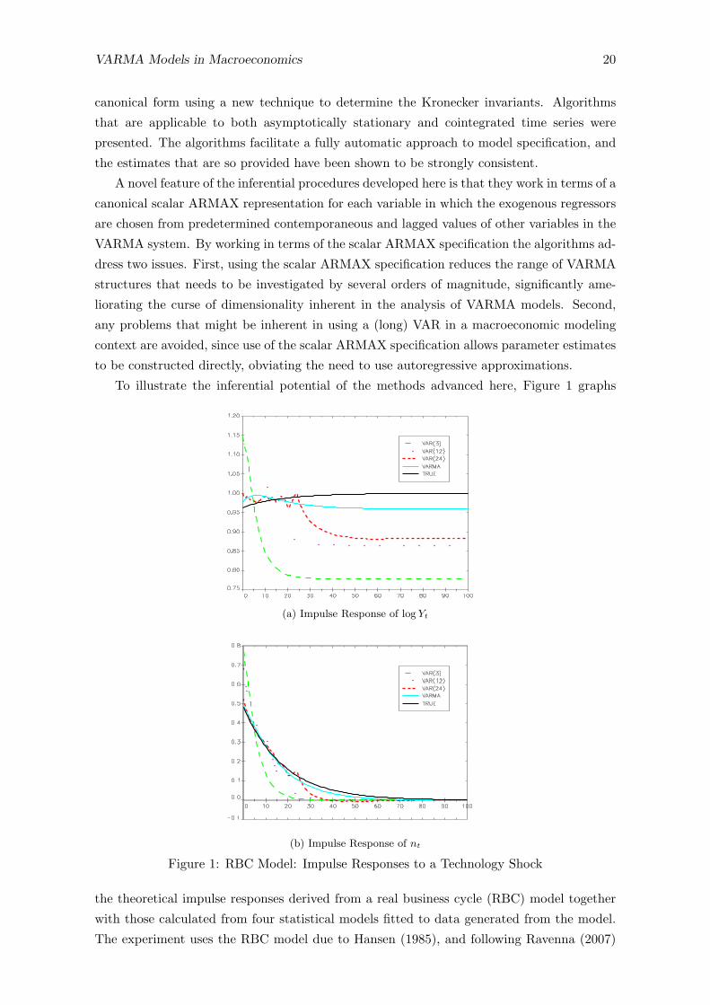
To illustrate the inferential potential of the methods advanced here, Figure 1 graphs
(a) Impulse Response of log Yt
(b) Impulse Response of nt
Figure 1: RBC Model: Impulse Responses to a Technology Shock
the theoretical impulse responses derived from a real business cycle (RBC) model together
with those calculated from four statistical models fitted to data generated from the model.
The experiment uses the RBC model due to Hansen (1985), and following Ravenna (2007)
VARMA Models in Macroeconomics 21
and Erceg, Guerrieri and Gust (2005) takes the capital stock as unobservable and treats
total output, Yt, and hours worked, nt, as the observable variables available for empirical
modelling. The model was calibrated as in Ravenna (2007) and Erceg et al. (2005) and it can
be shown (Yao and Kam, 2011) that the parameter values imply that the data generating
mechanism for yt = (nt,∆log Yt)′ has the representation(
1− 0.941B −1.045B
−0.770 + 0.724B 1
)yt =
(1− 0.250B −0.917B
−0.770 1
)εt , (9.1)
a bivariate ARMAE({1, 1}) process where the elements of the innovation εt equal linear
combinations of two uncorrelated exogenous structural shocks, a technology shock and a
labor supply shock. The four statistical models comprise an estimated VARMA model and
three VAR approximations constructed from a realization of 20000 observations on yt.
For each model the transformation from the innovations to the structural shocks is ob-
tained using the Blanchard and Quah (1989) identification strategy. Neither structural shock
has a permanent impact on either component of yt, since yt is stationary, and the long run
identifying restrictions imply that a labor supply shock has no long run effect on the level of
Yt, while the opposite is true for a technology shock.
Preliminary analysis of the raw simulated data nt and Yt, t = 1, . . . , T = 20000, in-
dicated that yt = (nt,∆log Yt)′ could be treated as a stationary process. An augmented
Dickey–Fuller test unequivocally rejected the hypothesis that nt was a unit root process at
all conventional significance levels, whereas the same was not true of log Yt, and ϱT unam-
biguously indicated that nt and log Yt have a cointegrating rank of one. The VARMA model
for yt was correctly identified as an ARMAE({1, 1}), and eliminating redundant parameters
using the rules outlined in Athanasopoulos and Vahid (2008) gave the following estimated
structure (1− 0.941B −1.003B
−0.785 + 0.740B 1− 0.005B
)yt =
(1− 0.257B −0.870B
−0.785 1
)εt (9.2)
when the resulting model was fitted using FIML. The VAR approximations were estimated
using (Gaussian) QML with different autoregressive orders, h, chosen by reference to AIC,
BIC and HQ, giving h = 24, 3 and 12 respectively.
Given the proximity of the parameter values in (9.2) to those in (9.1) it is perhaps not
surprising to find that the VARMA modelling procedure has produced reasonable estimates
of the impulse response functions, and it is of interest to note that the impulse responses
generated from an unconstrained ARMAE({1, 1}) model are almost indistinguishable from
those generated from (9.2). The worst fitting impulse response profile from the VARMA
model is that estimating the impact of a technology shock on total output, but even here
the long run effect is under estimated by less than 5%.
It is clear from both panels in Figure 1, however, that the autoregressive approximations
do not mimic the true dynamics of the theoretical model very well, even with the longest lag
length. Interestingly enough, increasing the value of h does little to improve the general shape
of the VAR impulse response estimates, it merely serves to increase the minor oscillations
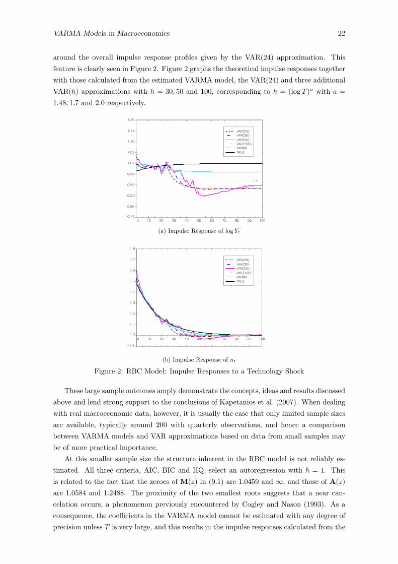
VARMA Models in Macroeconomics 22
around the overall impulse response profiles given by the VAR(24) approximation. This
feature is clearly seen in Figure 2. Figure 2 graphs the theoretical impulse responses together
with those calculated from the estimated VARMA model, the VAR(24) and three additional
VAR(h) approximations with h = 30, 50 and 100, corresponding to h = (log T )a with a =
1.48, 1.7 and 2.0 respectively.
(a) Impulse Response of log Yt
(b) Impulse Response of nt
Figure 2: RBC Model: Impulse Responses to a Technology Shock
These large sample outcomes amply demonstrate the concepts, ideas and results discussed
above and lend strong support to the conclusions of Kapetanios et al. (2007). When dealing
with real macroeconomic data, however, it is usually the case that only limited sample sizes
are available, typically around 200 with quarterly observations, and hence a comparison
between VARMA models and VAR approximations based on data from small samples may
be of more practical importance.
At this smaller sample size the structure inherent in the RBC model is not reliably es-
timated. All three criteria, AIC, BIC and HQ, select an autoregression with h = 1. This
is related to the fact that the zeroes of M(z) in (9.1) are 1.0459 and ∞, and those of A(z)
are 1.0584 and 1.2488. The proximity of the two smallest roots suggests that a near can-
celation occurs, a phenomenon previously encountered by Cogley and Nason (1993). As a
consequence, the coefficients in the VARMA model cannot be estimated with any degree of
precision unless T is very large, and this results in the impulse responses calculated from the
VARMA Models in Macroeconomics 23
estimated VARMA model tracking their VAR(1) approximation counterparts fairly closely
when T = 200, the performance of both being equally disappointing. Changing the pa-
rameter settings in the Hansen (1985) RBC model does little to alter these small sample
properties and highlights a challenging problem: Even though a theoretical model might
lead to a VARMA data generating mechanism, with insufficient observations it may be hard
to distinguish inferences based on VARMA models from those produced using VAR approx-
imations. Such outcomes are in accord with the findings of Kascha and Mertens (2009), who
suggest that the disadvantages of using VAR approximations rather than VARMA models
may therefore be over stated.
Recent work of Yao and Kam (2011) indicates, however, that behaviour of the type seen
above when T = 20000 can also be observed at sample sizes as small as T = 200. They
consider a two sector business–cycle monetary–search model that is an adaptation of Hansen
(1985) along the lines of Lagos and Wright (2005). Their model nests the one used here
and introduces more complicated interactions that result in the observed variables having a
more complex stochastic structure. Yao and Kam (2011) confirm that with large samples the
true ARMAE(ν) form is identified almost surely and that the VARMA modelling procedure
can produce quite precise impulse response function estimates. Their results also show that
VARs can yield poor approximations in spite of T being large (c.f. Chari et al., 2007).
Furthermore, Yao and Kam (2011) find that even at small sample sizes VARMA models
yield better estimates of the dynamics of their true business–cycle monetary–search model
than VAR approximations.
In summary, existing experimental evidence on the relative merits of using VARMA mod-
els vis–a–vis VAR approximations for macroeconomic modelling indicates that performance
is critically influenced by the sample size examined and, perhaps less obviously but possibly
more importantly, by the choice of economic model underlying the simulated data generating
mechanism. When taken together the overall conclusions are at best inconclusive. Although
asymptotic properties and results of the type presented in this paper can give an indication
of the likely behaviour of the procedures, their scope may be limited to very large samples
and additional insight into performance in small finite sample situations is needed. It is
hoped to present some guidance on the latter via more extensive simulation experiments and
empirical applications elsewhere.
Acknowledgement: I am grateful to George Athanasopoulos and Farshid Vahid for help-
ful and constructive comments on a previous version of this paper. I am also indebted to
Wenying Yao for conducting the numerical work reported above and for permission to refer-
ence the draft working paper with Tim Kam. Financial support by the Australian Research
Council under grant DP-0984399 is gratefully acknowledged.
References
Akaike, H. (1974a). A new look at the statistical model identification. IEEE-Transactions
on Automatic Control AC-19 716–723.
VARMA Models in Macroeconomics 24
Akaike, H. (1974b). Stochastic theory of minimal realization. IEEE Transactions on
Automatic Control AC-19 667–674.
Athanasopoulos, G., Poskitt, D. S. and Vahid, F. (2010). Two canonical VARMA
forms: Scalar component models vis-a-vis the Echelon form. Econometric Reviews In
Press.
Athanasopoulos, G. and Vahid, F. (2008). A complete VARMA modelling methodology
based on scalar components. Journal of Time Series Analysis 29 533–554.
Bartel, H. and Lutkepohl, H. (1998). Estimating the kronecker indices of cointegrated
Echelon-form VARMA models. Econometrics Journal 1 76–99.
Bingham, E. O. (1974). The Fast Fourier Transform. Prentice Hall, Englewood Cliffs.
Blanchard, O. J. and Quah, D. (1989). The dynamic effects of aggregate demand and
supply disturbances. American Economic Review 79 655–73.
Box, G. E. P. and Tiao, G. C. (1977). A canonical analysis of multiple time series.
Biometrika 64 355–365.
Brillinger, D. R. (1975). Time Series: Data Analysis and Theory. Holt, Rienhart and
Winston, New York.
Chari, V. V., Kehoe, P. J. and McGrattan, E. R. (2007). Are structural VARs with
long-run restrictions useful in developing business cycle theory? Federal Reserve Bank of
Minneapolis, Research Department Staff Report 364 .
Christiano, L. J., Eichenbaum, M. and Vigfusson, R. (2006). Assessing structural
VARs. NBER Macroeconomics Annual 1–106.
Cogley, T. and Nason, J. M. (1993). Impulse dynamics and propagation mechanisms in
a real business cycle model. Economics Letters 43 77–81.
Cooley, T. and Dwyer, M. (1998). Business cycle analysis without much theory. A look
at structural VARs. Journal of Econometrics 83 57–88.
Dahlhaus, R. (1988). Small sample effects in time series analysis: A new asymptotic theory
and a new estimate. Annals of Statistics 16 808–841.
Del Negro, M. and Schrfheide, F. (2004). Priors from general equilibrium models for
VARs. International Economic Review 45 643–673.
Doan, T., Litterman, R. and Sims, C. (1984). Forecasting and conditional projection
using realistic prior distributions. Econometric Reviews 3 1–10.
Engle, R. F. and Granger, C. W. J. (1987). Co-integration and error correction: Rep-
resentation, estimation, and testing. Econometrica 55 251–276.
VARMA Models in Macroeconomics 25
Erceg, C. J., Guerrieri, L. and Gust, C. (2005). Can long-run restrictions identify
technology shocks? Journal of the European Economic Association 3 1237–1278.
Fernandez-Villaverde, J., Rubio-Ramırez, J. F., Sargent, T. J. and Watson,
M. W. (2007). ABC’s (and D)’s of understanding VARs. The American Economic Review
97 1021–1026.
Fry, R. and Pagan, A. (2005). Some issues in using VARs for macroeconometric research.
CAMA Working Paper Series 19/2005, Australian National University .
Hannan, E. J. (1971). Multiple Time Series. J. Wiley, New York.
Hannan, E. J. and Deistler, M. (1988). The Statistical Theory of Linear Systems. Wiley,
New York.
Hannan, E. J. andKavalieris, L. (1984). Multivariate linear time series models. Advances
in Applied Probability 16 492–561.
Hannan, E. J. and Quin, B. G. (1979). The determination of the order of an autoregres-
sion. Journal of Royal Statistical Society B 41 190–195.
Hannan, E. J. and Rissanen, J. (1982). Recursive estimation of autoregressive-moving
average order. Biometrica 69 81–94.
Hansen, G. D. (1985). Indivisible labor and the business cycle. Journal of Monetary
Economics 16 309–327.
Johansen, S. (1995). Likelihood-based Inference on Cointegrated Vector Auto-regressive
Models. Oxford University Press, Oxford.
Kapetanios, G., Pagan, A. and Scott, A. (2007). Making a match: combining theory
and evidence in policy-oriented macroeconomic modelling. Journal of Econometrics 136
565–594.
Kascha, C. and Mertens, K. (2009). Business cycle analysis and varma models. Journal
of Economic Dynamics and Control 33 267 – 282.
Lagos, R. and Wright, R. (2005). A unified framework for monetary theory and policy
analysis. Journal of Political Economy 113 463–484.
Lutkepohl, H. (2005). The New Introduction to Multiple Time Series Analysis. Springer-
Verlag, Berlin.
Lutkepohl, H. and Claessen, H. (1997). Analysis of cointegrated VARMA processes.
Journal of Econometrics 80 223–239.
Nsiri, S. and Roy, R. (1992). On the identification of ARMA echelon form models. Cana-
dian Journal of Statistics 20 369–386.

VARMA Models in Macroeconomics 26
Paulsen, J. and Tjøstheim, D. (1985). On the estimation of residual variance and order
in autoregressive time series. Journal of the Royal Statistical Society B-47 216–228.
Poskitt, D. S. (1992). Identification of Echelon canonical forms for vector linear processes
using least squares. The Annals of Statistics 20 195–215.
Poskitt, D. S. (2000). Strongly consistent determination of cointegrating rank via canonical
correlations. Journal of Business and Economic Statistics 18 71–90.
Poskitt, D. S. (2003). On the specification of cointegrated autoregressive moving-average
forecasting systems. International Journal of Forecasting 19 503–519.
Poskitt, D. S. (2005). A note on the specification and estimation of ARMAX systems.
Journal of Time Series Analysis 26 157–183.
Poskitt, D. S. (2006). On the identification and estimation of nonstationary and cointe-
grated ARMAX systems. Econometric Theory 22 1138–1175.
Poskitt, D. S. and Chung, S. (1996). Markov chain models, time series analysis and
extreme value theory. Advances in Applied Probability 28 405–425.
Potscher, B. M. (1983). Order estimation in arma-models by lagrangian multiplier tests.
Annals of Statistics 11 872–885.
Ravenna, F. (2007). Vector autoregressions and reduced form representations of DSGE
models. Journal of Monetary Economics 54 2048–2064.
Schwarz, G. (1978). Estimating the dimension of a model. Annals of Statistics 6 461–464.
Sims, C. A. (1980). Macroeconomics and reality. Econometrica 48 1–48.
Smith, A. (1993). Estimating nonlinear time series models using simulated vector autore-
gressions. Journal of Applied Econometrics 8 563–584.
Stoica, P., Soderstrom, T. and Friedlander, B. (1985). Optimal instrumental vari-
ables estimates of the AR parameters of an ARMA process. IEEE Transactions on Auto-
matic Control AC–30 1066–1074.
Tiao, G. C. and Tsay, R. S. (1989). Model specification in multivariate time series (with
discussions). Journal of the Royal Statistical Society B 51 157–213.
Tjøstheim, D. and Paulsen, J. (1983). Bias of some commonly-used time series estimates.
Biometrika 70 389–399.
Wallis, K. (1977). Multiple time series analysis and the final form of econometric models.
Econometrica 45 1481–1497.
Yao, W. and Kam, T. (2011). Reassessing business-cycle VAR and VARMA models.
Monash University, Draft Working Paper.
VARMA Models in Macroeconomics 27
Appendix: Proofs
Proof of Lemma 3.1: That ut is a moving-average process of order p is obvious from
expression (1.2). Now let ej = (0, . . . , 0, 1, 0, . . . , 0)′ denote the j’th v element Euclidean
basis vector. From standard results on linear filtering we know that the spectral density of
νt = e′jut is
Sν(ω) =1
2πe′jM(ω)ΣM(ω)∗ej ,
with corresponding autocovariance generating function
ρ(z) =
n∑s=−n
ρszs
= e′jM(z)ΣM(z−1)′ej ,
where n = nj . The remainder of the proof is standard. The polynomial znρ(z) has 2n roots
and since the coefficients ρs = ρ−s, s = 1, . . . , n, of ρ(z) are real, the roots are real or occur
in complex conjugate pairs. Now, ρ(ω) = 2πSν(ω) > 0, −π < ω ≤ π, so ρ(z) has no zeroes
on the unit circle and we may number and group the roots into two sets {ζ1, . . . , ζn} and
{ζ−11 , . . . , ζ−1
n } such that |ζs| < 1, s = 1, . . . , n. Hence we can construct the operator
m(z) = m0
n∏s=1
(1− ζsz)
where m0 = {∏(−ζs)ρn}
12 such that
ρ(z) = ρnz−n
n∏s=1
(1− ζsz)(1− ζ−1s z)
= m(z)m(z−1) .
Thus we can select n roots of ρ(z) to construct µ(z) = 1 + µ1z + . . . + µnzn such that
ρ(z) = σ2ηµ(z)µ(z
−1), where µ(z) = m(z)/m0 and σ2η = m2
0, and the roots are chosen in
such a way that µ(z) = 0, |z| ≤ 1. The existence of the white noise process ηt providing
a moving-average representation of νt now follows from the spectral factorization theorem,
Rozanov (1967, Theorem 9.1, p. 41) (c.f. Lutkepohl, 2005, §11.6). 2
Proof of Proposition 3.1: To begin, recall that for yt ordered according to the Kronecker
invariants the echelon form in (2.1) is such that A0 = M0 is lower triangular and the system
representation is (contemporaneously) recursive. Let a(z) = e′jA(z) denote the nonzero
coefficients in the jth row of A(z). Then, for the jth equation of (1.2) we have
a(B)yt = yjt +
j−1∑i=1
aji,0yit +v∑
i=1
nj∑s=1
aji,syit−s = ujt (A.1)
where, by Lemma 3.1,
ujt = νt = ηt + µ1ηt−1 + . . .+ µnηt−n . (A.2)
VARMA Models in Macroeconomics 28
Setting zt = yjt and reorganizing (A.1), adopting the notational conventions αs = ajj,s,
s = 1, . . . , n = nj , βi = aji,0, i = 1, . . . , j − 1, and βi,s = aji,s, i = 1, . . . , v, i = j,
s = 1, . . . , n, now gives us the scalar ARMAX specification in (3.2).
To show that a(z) and µ(z), and hence the polynomials α(z), β(z) and µ(z), are coprime,
assume otherwise. Then we could cancel the common factors in the representation a(B)yt =
µ(B)ηt obtained by combining (A.1) and (A.2) to give a(B)yt = µ(B)ηt where δ[a, µ] < nj .
Implementing the same technique as employed in Poskitt (2005, pp. 179-180), we could now
use rows 1, . . . , j − 1 and j + 1, . . . , v of (1.2), together with a(B)yt = µ(B)ηt, to construct
a unimodular matrix U(z) = I and an operator pair [A(z) : M(z)] ∈ ARMAE(ν), with
multi-index ν = {n1, . . . , nv}, nj ≤ nj , such that [A(z) : M(z)] = U(z)[A(z) : M(z)],
contradicting Assumption 2.
Finally, it is obvious that the lagged values yit−s, i = 1, . . . , v, i = j, s = 1, . . . , n, are
predetermined. That the same is true of the contemporaneous regressors yit, i = 1, . . . , j−1,
follows from the fact that the structure is recursive and we can orthogonalize the innovation
process whilst maintaining both the recursive structure and the moving average row degrees.
To verify this, let Σ = CDC′ denote the Choleski decomposition of Σ where C is lower
triangular with unit leading diagonal elements and D = diag(d12 . . . , d2v). Then wt = C−1εt
is a martingale difference innovation sequence with covariance matrix D and we can rewrite
the ARMA system in (1.2) as
A0yt +
p∑s=1
Asyt−s = L0wt +
p∑s=1
Lswt−s . (A.3)
where L0 = M0C is again lower triangular with unit leading diagonal elements, and because
pre–multiplication by Ms reproduces zero-row structure, each Ls = MsC, s = 1, . . . , n, has
the same null rows as the corresponding Ms. From the jth equation of (A.3) we now have
ujt = wjt +
j−1∑i=1
lji,0wit +
v∑i=1
nj∑s=1
lji,swit−s . (A.4)
Thus, from (A.1) and (A.4) we see that in addition to wit, the variable yit depends at most
on w1t, . . . , wi−1t. Since by construction the elements of wt are mutually uncorrelated, it
follows that for i = 1, . . . , j − 1 we have E[yitwjt | Ft−1] = 0, as required. 2
Proof of Theorem 5.1: The proof of Theorem 5.1 is based on the following lemmas.
Lemma A.1 Suppose that yt is an ARMA process satisfying Assumptions 1 and 2′ and
assume that (r(i), nr(i)) = (r(i)0, n0r(i)) for i = j+1, . . . , v. Let a†(z) =
∑ns=0 a
†szs where the
coefficients a†s, s = 0, . . . , n belong to the solution set of the equation system
n∑s=0
a†sΓy(r + s) = 0, r = n+ 1, . . . , 2n . (A.5)
Set α†(z) = a†(z)ej and β†(z) = a†(z)(I−eje
′j). Given α†(z) and β
†(z), let µ†(z) be formed
VARMA Models in Macroeconomics 29
from ∫ π
−π
n∑s=0
µ†s
a†(ω)Sy(ω)a†(ω)∗
S†v(ω)2
expıω(s−r) dω = 0, r = 1, . . . , n , (A.6)
where
S†v(ω) =
1
2π
∫ π
−π
n∑r=−n
a†(θ)Sy(θ)a†(θ)∗ expı(ω−θ)r dθ . (A.7)
Then, provided that for i = j+1, . . . , v the Kronecker invariant pairs satisfy {r(i)T , nr(i)T } =
{r(i)0, n0r(i)}, we have:
(i) If n < nr(j)0, α(z) = α†(z)+O(QT ),β(z) = β
†(z)+O(QT ) and µ(z) = µ†(z)+O(QT )
uniformly in |z| ≤ 1 where QT = (loglogT/T )1/2;
(ii) If n = nr(j)0, α(z) = α0(z)+O(QT ),β(z) = β
0(z)+O(QT ) and µ(z) = µ0(z)+O(QT )
uniformly in |z| ≤ 1;
(iii) If n > nr(j)0, α(z) = ϕ(z)α0(z) + O(QT ),β(z) = ϕ(z)β
0(z) + O(QT ) and µ(z) =
ϕ(z)µ0(z)+O(QT ) uniformly in |z| ≤ 1 where ϕ(z) = 1+ϕ1z+. . .+ϕrzr, r = n−nr(j)0,
and ϕ(z) = 0, |z| ≤ 1.
Proof of Lemma A.1: From Theorem 5.3.2 of Hannan and Deistler (1988) we know that
∥Cy(r) − Γy(r)∥ = O(QT ), r = 0, . . . , HT ≤ (log T )a, a < ∞. From (4.1) and (A.5) we
recognize that a(z) and a†(z) correspond to the solutions of systems of linear equations in
which the coefficient matrices of the two systems differ by terms of order O(QT ). Moreover,
the coefficient matrix of the system of equations is nonsingular by a direct application of
Theorem 6.2.5 of Hannan and Deistler (1988). We can therefore conclude that as − a†s =
O(QT ), s = 0, . . . , n. See also Theorem 6.2.4 of Hannan and Deistler (1988). Treating the
polynomial operators as elements of the Hardy space H2, the space of functions analytic for
|z| < 1 and square integrable on |z| = 1, now yields the result that
∥α(z)− α†(z)∥2 = ∥(a(z)− a†(z))ej∥2 =n∑
s=0
(αs − α†s)
2 = O(Q2T )
and
∥β(z)− β†(z)∥2 = ∥(a†(z)− a†(z))(I− eje
′j)∥2
=
j−1∑i=1
(βi − β†
i )2 +
v∑i=1i=j
n∑s=1
(βi,s − β†
i,s)2 = O(Q2
T ) .
A parallel argument to that just employed will show that µ(z) = µ†(z)+O(QT ), |z| ≤ 1,
if it can be verified that the difference in the coefficient matrices of the two equation systems
that define the operators µ(z) and µ†(z) are, likewise, O(QT ). To establish the latter, observe
VARMA Models in Macroeconomics 30
that
Cv(r) =
n∑s=0
n∑u=0
asCy(r + s− u)a′u=
n∑s=0
n∑u=0
(a†s +O(QT )
)(Γy(r + s− u) +O(QT )
)(a†u +O(QT )
)′=
n∑s=0
n∑u=0
a†sΓy(r + s− u)a†′u +O(QT )
= γ†v(r) +O(QT ) , say, (A.8)
where γ†v(r) =∫ π−π a
†(ω)Sy(ω)a†(ω)∗ exp−ıωr dω. From (A.8) it follows directly that
Sv(ω) =
1
2π
n∑s=−n
Cv(s) exp(ıωs)
=1
2π
n∑s=−n
(γ†v(s) +O(QT )
)exp(ıωs)
= S†v(ω) +O(QT )
uniformly in ω ∈ [−π, π].
LetH(ω) = a(ω)/|Sv(ω)| and set H†(ω) = a†(ω)/|S†
v(ω)|. It is established below thatH(ω) and H†(ω) belong to L2, with Fourier coefficients that decline at a geometric rate, and
that∫ π−π ∥
H(ω)− H†(ω)∥2dω = O(Q2
T ). Now set
γi†v(r) =
∫ π
−πH†(ω)Sy(ω)H
†(ω)∗ exp(−ıωr)dω .
Then, by definition,
|Civ(r)− γi†v(r)| =∣∣∣ ∫ π
−π
( H(ω)Iy(ω)
H(ω)∗ − H†(ω)Sy(ω)H
†(ω)∗)exp(−ıωr)dω
∣∣∣ , (A.9)
and suppressing the argument ω for convenience we have
HIy
H
∗− H†SyH
†∗ =(H− H†)Iy(
H− H†)∗ + (
H− H†)IyH
†∗
H†Iy(H− H†)∗ + H†(Iy − Sy)H
†∗ . (A.10)
Substituting (A.10) into (A.9) we can now bound |Civ(r)− γi†v(r)| by the sum of four terms.
The first term is∣∣∣ ∫ π
−π(H− H†)Iy(
H− H†)∗ exp(−ıωr)dω
∣∣∣ ≤ ∫ π
−π(H− H†)Iy(
H− H†)∗dω . (A.11)
VARMA Models in Macroeconomics 31
Applying the Cauchy-Schwartz inequality to the right hand side integrand in (A.11), recog-
nizing that Iy is Hermitian positive semi-definite, we find that∫ π
−π(H− H†)Iy(
H− H†)∗dω =
1
2πT
∫ π
−π|( H− H†)Zy(ω)|2dω
≤∫ π
−π∥( H− H†∥2tr{Iy}dω
≤ supω∈[−π,π]
tr{Iy}∫ π
−π∥( H− H†∥2dω
= O(log T )O(Q2T ) ,
since lim supT→∞[supω∈[−π,π] tr{Iy(ω)}/ log T ] ≤ supω∈[−π,π] 2tr{Sy(ω)} (Brillinger, 1975,
Theorem 5.3.2.) Similarly, the second term,∣∣∣ ∫ π
−π(H − H†)IyH
†∗ exp(−ıωr)dω∣∣∣ , and the
third term,∣∣∣ ∫ π
−π H†Iy(
H− H†)∗ exp(−ıωr)dω
∣∣∣ , are both bounded by
∫ π
−π|H†Iy(
H− H†)∗| ≤
∫ π
−π
(H†IyH
†∗)1/2(
(H− H†)Iy(
H− H†)∗
)1/2
dω
≤∫ π
−π
(H†IyH
†∗)dω
∫ π
−π
((H− H†)Iy(
H− H†)∗
)dω
≤ ( supω∈[−π,π]
tr{Iy})2∫ π
−π∥H†∥2dω
∫ π
−π∥( H− H†∥2dω
= (O(log T ))2O(Q2T ) .
The fourth term is∣∣∣ ∫ π
−π H†(Iy − Sy)H
†∗ exp−ı ωr dω∣∣∣, which equals
∣∣∣ ∞∑u=−∞
∞∑s=−∞
h†u[Cy(r + u− s)− Γy(r + u− s)]h†′
s
∣∣∣≤
∞∑u=−∞
∞∑s=−∞
∣∣∣h†u[Cy(r + u− s)− Γy(r + u− s)]h†′
s
∣∣∣≤
∞∑u=−∞
∞∑s=−∞
∥h†u∥ · ∥Cy(r + u− s)− Γy(r + u− s)∥ · ∥h†
s∥ , (A.12)
wherein we set Cy(τ) = 0, |τ | ≥ T , and h†u =
∫ π−π H
†(ω) exp−ı ωu dω, u = 0,±1, . . .. Since
there exists a constant κ > 0 and a parameter λ, 0 < λ < 1, such that ∥h†u∥ < κλ|u|, the
right hand side of equation (A.12) is less than or equal to
κ2∑
|u|<c log T
∑|s|<c log T
∥Cy(r + u− s)− Γy(r + u− s)∥λ|u|+|s|
+ κ2(∥Cy(0)∥+ ∥Γy(0)∥)∑
|u|≥c log T
∑|s|≥c log T
λ|u|+|s| . (A.13)
By Theorem 5.3.2 of Hannan and Deistler (1988), the order of magnitude of the first term
in this expression is O(QT )4κ2(1−λc log T )2/(1−λ)2 = O(QT ). The second term is bounded
by a constant times 4κ2λ2c log T /(1− λ)2, which is of order O(T−1) for any c ≥ −1/(2 log λ).
VARMA Models in Macroeconomics 32
Hence we can conclude that the coefficient matrices of the two equation systems that
define the operators µ(z) and µ†(z) differ by terms that are of order O(QT ) or smaller, as
was required to be shown.
(i) The first statement of the lemma now follows without further ado.
(ii) When n = n0r(j) it is readily verified that a†(z) = a0(z) provides the solution to (A.5).
By definition a0(z) = e′jA0(z), from which it follows that a0(ω)K0(ω) = e′jM
0(ω) where
a0(ω) = a0(z)∣∣z=eıω
and, given that Sy(ω) = (2π)−1K0(ω)Σ0K0(ω)∗,
a0(ω)Sy(ω) = (2π)−1e′jM0(ω)Σ0K0(ω)∗ . (A.14)
From (A.14) we can conclude that∫ π−π a
0(ω)Sy(ω) exp−ıωu dω = 0 for u > n and therefore
∫ π
−πa0(ω)Sy(ω) exp
−ıωr dω =
n∑s=0
a0sΓy(r + s) = 0 , r = n+ 1, . . . , 2n .
Similarly, the quadratic form
a0(ω)Sy(ω)a0(ω)∗ = (2π)−1e′jM
0(ω)Σ0M0(ω)∗ej
= (2π)−1(σ0η)
2|µ0(ω)|2 .
Substituting a†(ω) = a0(ω) into (A.7) we find that the equation system (A.6) corresponds to
the Yule-Walker equations constructed from the (inverse) power spectrum 2π/(σ0η)
2|µ0(ω)|2,and hence that µ†(z) = µ0(z).
We are therefore lead to the conclusion that α(z) = αo(z)+O(QT ),β(z) = β
o(z)+O(QT )
and µ(z) = µo(z) +O(QT ), verifying the strong consistency claimed in Remark 1.
(iii) Now consider the case n > n0r(j). Using the relationship in (A.14) it is straightforward
to show that the solutions to Eq. (A.5) are characterized by operators of the form a†(z) =
ϕ(z)a0(z) where ϕ(z) = 1+ϕ1z+. . .+ϕrzr, r = n−n0
r(j). Moreover, since∑n
s=0 a†jΓy(s−j) =
0, s ≥ n,
|n∑
j=0
a†jCy(s− j)| ≤n∑
j=0
∥a†j∥∥Cy(s− j)− Γy(s− j)∥ = O(QT )
n∑j=0
∥a†j∥.
Thus for T sufficiently large we can determine a measurable solution a(z) to (4.1) such that,
with arbitrarily large probability, a(z) = ϕ(z)a0(z) +O(QT ) where ϕ(z) = 0, |z| ≤ 1.
Substituting a†(ω) = ϕ(ω)a0(ω) into (A.7) we find that
S†v(ω) =
1
2π
n∑r=−n
∫ π
−π|ϕ(θ)|2a0(θ)Sy(θ)a
0(θ)∗ expı(ω−θ)r dθ
=(σ0
η)2
2π|ϕ(ω)|2|µ0(ω)|2
VARMA Models in Macroeconomics 33
and hence, via (A.6), that µ(z) = µ†(z) +O(QT ) where the coefficients of µ†(z) are derived
from the Yule-Walker equations
n∑j=0
µ†j γi
†v(r + j) = 0 , r = 1, . . . , n,
with
γi†v(s) =
∫ π
−π
2π exp−iωs
(σ0η)
2|ϕ(ω)µ0(ω)|2dω .
This gives the desired conclusion.
To complete the proof it remains to be shown thatH, H† ∈ L2, with Fourier coefficients
that decline at a geometric rate, and that ∥ H− H†∥2 = O(Q2T ).
Consider H†. Given that a†(z) is polynomial it is sufficient to show that S†v(ω)−2 is
absolutely integrable to verify that H† ∈ L2. By Weierstrass’s approximation theorem, for
any ϵ > 0, no matter how small, there exists a polynomial p(z) =∑
j≥0 pjzj , with p(z) = 0,
|z| ≤ 1, such that |S†v(ω)2 − |p(ω)|2| ≤ ϵ uniformly in ω. Clearly, p−1 ∈ L2 and∫ π
−π
1
S†v(ω)2 + ϵ
dω =
∫ π
−π
1
|p(ω)|2+
1
|p(ω)|2
{|p(ω)|2
S†v(ω)2 + ϵ
− 1
}dω
≤∫ π
−π
1
|p(ω)|2
∣∣∣∣∣1 + {|p(ω)|2 − S†v(ω)2 − ϵ}
S†v(ω)2 + ϵ
∣∣∣∣∣ dω≤ 3
∫ π
−π
1
|p(ω)|2dω < ∞ .
Letting ϵ → 0 we can therefore conclude from Lebesgue’s monotone convergence theorem
that S†v(ω)−2 is absolutely integrable and hence that H† ∈ L2. Moreover, if Hp(ω) =
a†(ω)/|p(ω)|, then Hp ∈ L2 and Hp can be expanded in a mean–square convergent Fourier
series, (2π)−1∑
hps exp(ıωs) say, where ∥hp
s∥ → 0 at a geometric rate as |s| → ∞. Now,
∥H† − Hp∥2 =
∫ π
−π
∥a†∥2
S†2v
∣∣∣|p| − |S†v|∣∣∣2
|p|2dω
≤ ∥H†∥2 sup[−π,π]
ϵ2
|p|4, (A.15)
and ∥h†s∥ ≤ ∥hp
s∥+∥h†s− hp
s∥, implying that there exists a constant κ > 0 and a parameter λ,
0 < λ < 1, such that ∥h†s∥ < κλ|s|, since by Bessel’s inequality and (A.15) sups ∥h
†s− hp
s∥2 ≤∥H†− Hp∥2 → 0 as ϵ → 0. A parallel proof, replacing a† by a and S†
v bySv, also shows that
H ∈ L2, with Fourier coefficients that decline at a geometric rate.
Finally, ∥ H− H†∥2 = O(Q2T ) follows from the triangular inequality and the expansion
H− H† = (a− a†)
1
|Sv|+ a†
|S†v| − |Sv|
|SvS†v|
because ∥a(ω)− a†(ω)∥ = O(QT ) and
Sv(ω) = S†
v(ω) +O(QT ) uniformly in ω ∈ [−π, π]. 2
Lemma A.2 Suppose that yt is an ARMA process satisfying Assumptions 1 and 2′, and
VARMA Models in Macroeconomics 34
assume that for j = q+1, . . . , v the Kronecker invariant pairs {r(j)T , nr(j)T } = {r(j)0, n0r(j)}.
Then for all T sufficiently large
(i) σ2
η(n) >σ2
η(n+ 1) with probability one if n < n0r(q), and
(ii) if n ≥ n0r(q),
σ2
η(n)− σ2
η(n+ 1) = O(Q2T ) almost surely.
Proof of Lemma A.2: As observed in Remark 2, Step 2 corresponds to a Gauss-Newton
iteration designed to minimize
1
T
T∑t
η2t = ∫ π
−π
a(ω)Iy(ω)a(ω)∗|µ(ω)|2 dω +O((log T/T 1/2)) . (A.16)
Set
FT (n) = min{a(z),µ(z)}
∫ π
−π
a(ω)Iy(ω)a(ω)∗
|µ(ω)|2dω
where a(z) and µ(z) are of degree n. Clearly, FT (n + 1) ≤ FT (n). Now suppose that
FT (n+ 1) = FT (n). This implies that the function
F(a, b) =
∫ π
−π
|1− a expiω |2
|1− b expiω |2|a(ω)Zy(ω)|2
2πT |µ(ω)|2dω
is minimised at a = b, |b| < 1. Following the method of argument used by Potscher (1983,
pp. 877–878) in the proof of his Theorem 5.2 we find that this leads to the conclusion that
a(z)Zy(z)/µ(z) ≡ 1 and the ’transfer function’ Zy(z) is rational of degree n. But the order,
or McMillan degree, of Zy(z) =∑T
t=1 ytzt is T with probability one. Hence we can infer that
FT (n+ 1) < FT (n), reductio ad absurdum. Now set 0 < δn < (FT (n)− FT (n+ 1))/4. From
(A.16), which follows from Theorems 4.5.2 and 5.3.2 of Brillinger (1975), it follows that when
T is sufficiently large both the events σ2
η(n) > FT (n)−δn and σ2
η(n+1) < FT (n+1)+δn will
occur with probability arbitrarily close to one. Thus σ2
η(n)− σ2
η(n+ 1) > (FT (n)− FT (n+
1))− 2δn > 12(FT (n)− FT (n+ 1)) > 0, confirming the result in (i) for n < n0
r(q).
We will now establish that σ2
η(n) = T−1∑
η2t + O(Q2T ) whenever n ≥ n0
r(q), from which
the stated equality in (ii) follows directly. By definition,
σ2
η(n) =1
T
T∑t
η2t + n∑j=0
∆aj 1T
T∑t=1
ξt−j
ηt − n∑j=1
∆µj
1
T
T∑t=1
φt−jηt
=1
T
T∑t
η2t + T−1T∑t=1
(∆a(B)ξt −∆µ(B)φt)ηt , (A.17)
the residual mean squared error from regressing ηt on the derivative processes −ξt−j , j =
0, . . . , n, and φt−j , j = 1, . . . , n.
Consider first T−1∑T
tη2t . By Lemma A.1 a(z) = ϕ(z)a0(z) + O(QT ) and µ(z) =
ϕ(z)µ0(z) + O(QT ) uniformly in |z| where ϕ(z) ≡ 1 when n = n0r(q) and ϕ(z) = 0, |z| ≤ 1,
when n > n0r(q). Then
a0(z)
µ0(z)−a(z)µ(z) =
∑j≥0
ψ0jz
j
VARMA Models in Macroeconomics 35
where the ψ0j are O(QT ) and decline at a geometric rate, so that ∥ψ0
j∥ < O(QT )λj ,
j = 0, 1, 2, . . ., for some λ, 0 < λ < 1. This implies that |ηt − ηt| ≤ ∑j≥0 ∥ψ
0j∥ · ∥yt−j∥ ≤
O(QT )∑
j≥0 λj∥yt−j∥ and hence that T−1
∑(ηt − ηt)2 ≤ O(Q2
T )tr{Cy(0)}/(1 − λ)2. Fur-
thermore,
T−1T∑t=1
(ηt − ηt)ηt = a log T∑j=0
ψ0j [T
−1T∑t=1
yt−j ηt] +RT (A.18)
where the remainderRT is dominated byO(QT )(tr{Cy(0)}T−1∑
η2t )1/2λa log T /(1−λ). From
Proposition 3.1 we know that the variables in yt−j , j = 0, 1, . . . , a log T that are present in the
mean cross products T−1∑T
t=1 yt−j ηt occurring in (A.18) are predetermined relative to ηt.
From Theorem 5.3.1 of Hannan and Deistler (1988) it follows that these mean cross products
are O(QT ). This then leads to the conclusion that T−1∑T
t=1(ηt − ηct)ηt = O(Q2
T )(1 −λa log T )/(1− λ) +O(QT )λ
a log T /(1− λ). Taking a > −1/ log λ gives the result that
T−1∑η2t = T−1
∑η2t + T−1
∑(ηt − ηt)2 − 2T−1
T∑t=1
(ηt − ηt)ηt= T−1
∑η2t +O(Q2
T ) . (A.19)
Turning to the regression mean square, a similar argument to that just employed can
be used to establish that when n ≥ n0r(q) the mean cross products of ηt with the derivative
processesξt−j , j = 0, . . . , n, and φt−j , j = 1, . . . , n, are O(QT ). First,
T−1T∑t=1
ξt−j
ηt = T−1a log T∑s=0
ks{
T∑t=1
yt−j−sηt −T∑t=1
yt−j−s(ηt − ηt)}+RT (A.20)
where∑
s≥0ksz
s = 1/µ(z) and |ks| ≤ κλs, κ > 0, 0 < λ < 1. As above, Theorem 5.3.1
of Hannan and Deistler (1988) implies that T−1∑T
t=1 yt−j−sηt = O(QT ), and from what
has already been shown ∥T−1∑T
t=1 yt−j−s(ηt − ηt)∥ ≤ (tr{Cy(0)}T−1∑T
t=1(ηt − ηt)2)1/2 =
O(QT ). The norm of the right hand side summations in (A.20) is therefore bounded by
O(QT )2κ(1 − λa log T )/(1 − λ). The remainder RT =∑
s>a log TksT
−1∑T
t=1 yt−j−sηt can
be similarly bounded to give ∥RT ∥ ≤ κ(tr{Cy(0)}T−1∑T
t=1η2t )1/2λa log T /(1 − λ). Taking
a > −1/ log λ implies that ∥RT ∥ = O(T−1) and hence T−1∑T
t=1ξt−j
ηt = O(QT ). Second,
T−1T∑t=1
φt−jηt = T−1
a log T∑s=0
ks{
T∑t=1
yt−j−sηt −T∑t=1
yt−j−s(ηt − ηt)}+RT (A.21)
where∑
s≥0ksz
s = a(z)/µ(z)2 and ∥ks∥ ≤ κλs, κ > 0, 0 < λ < 1. An argument that
exactly parallels that used in the development immediately preceeding (A.21) leads to the
conclusion that T−1∑T
t=1φt−j
ηt = O(QT ).
Given that the parameter adjustments ∆aj , j = 0, . . . , n, and ∆µj , j = 1, . . . , n, can be
expressed as weighted sums of T−1∑ξt−j
ηt, j = 0, . . . , n, and T−1∑
φt−jηt, j = 1, . . . , n,
with weights that are almost surely O(1), it follows that ∥∆a(z)∥2 = O(Q2T ) and ∥∆µ(z)∥2 =
O(Q2T ).
VARMA Models in Macroeconomics 36
Applying the Cauchy-Schwartz inequality we can therefore conclude that when n ≥ n0r(q)
the regression mean square
T−1T∑t=1
(∆a(B)ξt −∆µ(B)φt)ηt = O(Q2
T ) . (A.22)
Substituting (A.19) and (A.22) into (A.17) produces the desired result, namely thatσ2
η(n) = T−1∑
η2t +O(Q2T ) when n ≥ n0
r(q). This completes the proof of Lemma (A.2). 2
Proof of Theorem 5.1: Lemma (A.2) (i) implies that when n < n0r(q)
lim infT→∞
log[σ2
η(n)/σ2
η(n+ 1)]> log(1 + ρ(n)(1− δ)) > 0
with probability one for any δ, 0 < δ < 1, where ρ(n) = σ2
η(n)/σ2
η(n + 1) − 1 > 0. The
assumption that pT (dq(n))/T → 0 a.s. as T → ∞ therefore implies that ICT (n+1) < ICT (n)
a.s. for n < n0r(q) because pT (dq(n))/(T log(1+ρ(1−δ))) → 0 a.s.. Hence lim infT→∞ nr(q)T ≥
n0r(q). When n ≥ n0
r(q), Lemma (A.2) (ii) implies
log[σ2
η(n)/σ2
η(n+ 1)]= log(1 +O(Q2
T )) = O(Q2T ) .
If lim infT→∞ pT (dq(n))/L(T ) > 0, then since dq(n) < dq(n+ 1)
ICT (n)− ICT (n+ 1)
L(T )=
TO(Q2T )
L(T )+
pT (dq(n))− pT (dq(n+ 1))
L(T )< 0 ,
implying that ICT (n + 1) > ICT (n) a.s. for n ≥ n0r(q) and lim supT→∞ nr(q)T ≤ n0
r(q).
Theorem (5.1) follows on directly. 2
Proof of Proposition 6.1: Since Proposition 3.1 depends on Assumption 2 and not the
more restrictive Assumption 2′ it holds in its entirety for the ARMAE(ν) representation
of the levels yt when yt is an ECARMAE(ν, ρ) cointegrated process. In order to couch
Proposition 3.1 in terms of the EC representation in (6.1) we apply the Beveridge-Nelson
decomposition before proceeding as in the development of (3.2) to give
b(B)△yt + π′yt−1 = ηt +
n∑s=1
µsηt−s , (A.23)
where b(z) = e′jB(z) and π′ = e′jCE. Now set △zt = e′j△yt. Then given Tc we can
manipulate (A.23) to produce expression (6.2) where α(z) = b(z)ej , β(z) = b(z)(I− eje′j)
and c′ = π′T′c(TcT
′c)
−1 = e′jF. Recall that in Proposition 3.1 the variables are assumed
to have been ordered according to the Kronecker invariants, and note that xct = Tcyt is
invariant to the ordering of the variables in yt. 2
Proof of Theorem 8.1: In what follows we will use the appendage of the subscript c
to denote quantities calculated by applying Stage 2 of Algorithm–ARMAE(ν, ϱ) to zt =
[△y′t,x
′c(t−1)]
′ rather than wt = [△y′t, ζ
′(t−1)]
′. Set D = diag(I,RT ). Then wt − Dzt =
VARMA Models in Macroeconomics 37
(0, (BT −RTT0c)yt−1) and
T−1T∑t=1
∥wt −Dzt∥2 = T−1tr[(BT −RTT0c)
T∑t=1
yt−1y′t−1(BT −RTT
0c)
′]
= O(Q2T ) (A.24)
where the order of magnitude in (A.24) follows by Lemma 3.1 and Lemma A1 (i) of Poskitt
(2000). Furthermore, Cw(r)−DCz(r)D′ equals
1
T
[0
∑Tt=r+1△yty
′t−r−1(BT −RTT
0c)
′∑Tt=r+1(BT −RTT
0c)yt−1△y′
t−r−1
∑Tt=r+1(BTyt−1y
′t−r−1B
′T −RTT
0cyt−1y
′t−r−1T
0′c R
′T )
]
and using the Cauchy–Schwartz inequality in conjunction with (A.24) to bound the nonzero
entries, having first rewritten the (2, 2) block as
T−1T∑
t=r+1
(BT −RTT0c)yt−1y
′t−r−1(BT −RTT
0c)
′+T−1T∑
t=r+1
(BT −RTT0c)yt−1y
′t−r−1T
0′c R
′T
+ T−1T∑
t=r+1
RTT0cyt−1y
′t−r−1(BT −RTT
0c)
′ ,
we find that
Cw(r)−DCz(r)D′ =
[0 O(QT )
O(QT ) O(QT )
](A.25)
uniformly in r. Using equation (A.25) we can now establish the following lemma.
Lemma A.3 Suppose that yt is an ECARMAE(ν, ρ) process satisfying Assumptions 1 and
2 and that ϱT = ϱ0. Then ∥d(z) − dc(z)D−1∥2 = O(Q2
T ) and ∥µ(z) − µc(z)∥2 = O(Q2T ),
|z| ≤ 1, whered(z) and µ(z), and dc(z) and µc(z), denote the operators obtained from the
coefficient values calculated by applying the first step of Stage 2 of Algorithm–ARMAE(ν, ϱ)
to wt and zt respectively.
Proof of Lemma A.3: Replacing Theorem 5.3.2 of Hannan and Deistler (1988), as used in
the proof of Lemma A.1, by (A.25), it follows from (7.1) that the coefficients ofd(z) and
dc(z)D−1 are derived from the solutions of nonsingular linear equation systems in which
the terms differ by order O(QT ). We can therefore conclude thatds −
dcsD
−1 = O(QT ),
s = 0, . . . , n, and hence that ∥d(z)− dc(z)D−1∥2 = O(Q2
T ), as required.
It now follows that
Ccv(r) =n∑
s=0
n∑u=0
dcsCz(r + s− u)
d′cu
=n∑
s=0
n∑u=0
(ds +O(QT )
)(DCz(r + s− u)D′
)(du +O(QT )
)′
=n∑
s=0
n∑u=0
dsCw(r + s− u)
d′u +O(QT )
= Cv(r) +O(QT ) , (A.26)
VARMA Models in Macroeconomics 38
and hence, by the same argument that follows (A.8),Scv(ω) =
Sv(ω) +O(QT ) uniformly in
ω.
LetHc(ω) =
dc(ω)/|
Scv(ω)|. By definition Cicv(r) =
∫ π−πHc(ω)Iz(ω)
Hc(ω)
∗ exp(−ıωr)dω,
and
|Cicv(r)−Civ(r)| =∣∣∣ ∫ π
−π
( Hc(ω)Iz(ω)
Hc(ω)
∗ − H(ω)Iw(ω)
H(ω)∗
)exp(−ıωr)dω
∣∣∣ . (A.27)
whereH(ω) =
d(ω)/|Sv(ω)|. Suppressing the argument ω for convenience, we can substitute
HcIz
H
∗c −
HIw
H
∗=HcD
−1DIzD′D′−1 H∗
c −HIw
H
∗
=(HcD
−1 − H)DIzD
′(HcD
−1 − H)∗ +
H(DIzD
′ − Iw)H
∗
+HDIzD
′(HcD
−1 − H)∗ + (
HcD
−1 − H)DIzD
′ H∗(A.28)
into (A.27) and bound |Cicv(r)− Civ(r)| by the sum of
I1 =∣∣∣ ∫ π
−π(HcD
−1 − H)DIzD
′(HcD
−1 − H)∗ exp(−ıωr)dω
∣∣∣ ,
I2 =∣∣∣ ∫ π
−π2ℜ{ HDIzD
′(HcD
−1 − H)∗} exp(−ıωr)dω
∣∣∣and
I3 =∣∣∣ ∫ π
−π
H(Iw −DIzD
′)H
∗exp(−ıωr)dω
∣∣∣ .
As in Lemma A.1,H,HcD
−1 ∈ L2, with Fourier coefficients that decline at a geometric rate,
and ∥ HcD−1 −
H∥2 = O(Q2T ). It follows that the first term
I1 ≤∫ π
−π(HcD
−1 − H)DIzD
′(HcD
−1 − H)∗dω
≤∫ π
−π∥ HcD
−1 − H∥2tr{DIzD
′}dω
≤ supω∈[−π,π]
tr{DIzD′}∥ HcD
−1 − H∥2
= O(log T )O(Q2T ) ,
and the second
I2 ≤ 2
∫ π
−π| HDIzD
′(HcD
−1 − H)∗|dω
≤ 2
∫ π
−π
( HDIzD
′ H∗)1/2((HcD
−1 − H)DIzD
′(HcD
−1 − H)∗
)1/2
dω
≤ 2
∫ π
−π
( HDIzD
′ H∗)dω
∫ π
−π
((HcD
−1 − H)DIzD
′(HcD
−1 − H)∗
)dω
≤ 2( supω∈[−π,π]
tr{DIzD′)2∥ H∥2∥ HcD
−1 − H∥2
= (O(log T ))2O(Q2T ) .
VARMA Models in Macroeconomics 39
The third term
I3 ≤∞∑
u=−∞
∞∑s=−∞
∣∣∣hu[Cw(r + u− s)−DCz(r + u− s)D′]h′s
∣∣∣ (A.29)
wherein Cw(τ) = Cz(τ) = 0, |τ | ≥ T . Since ∥hu∥ < κλ|u| the right hand side of (A.29) can
be bounded by
κ2∑
|u|<a log T
∑|s|<a log T
∥Cw(r + u− s)−DCz(r + u− s)D′∥λ|u|+|s|
+ κ2(∥Cw(0)∥+ ∥DCz(0)D∥)∑
|u|≥a log T
∑|s|≥a log T
λ|u|+|s| . (A.30)
The first term in (A.30) is O(QT )4κ2(1−λa log T )2/(1−λ)2 = O(QT ), by (A.25). The second
term is dominated by a constant times 4κ2λ2a log T /(1 − λ)2, and taking a ≥ −1/(2 log λ)
makes this term of order O(T−1).
The difference in the coefficient matrices of the two systems of Yule–Walker equations
that define the operators µ(z) and µc(z) have thus been shown to be O(QT ), and henceµ(z) = µc(z) +O(QT ), |z| ≤ 1, giving the desired result. 2
Lemma A.4 Suppose that yt is an ECARMAE(ν, ρ) process satisfying Assumptions 1 and
2 , and assume that ϱT = ϱ0 and that for j = q + 1, . . . , v the Kronecker invariant pairs
{r(j)T , nr(j)T } = {r(j)0, n0r(j)}. If σ2
η(n) and σ2
cη(n) denote the mean squared error values
obtained at the second step of Stage 2 of Algorithm–ARMAE(ν, ϱ) when the algorithm is
applied to wt and zt respectively, then for all T sufficiently large
(i) σ2
η(n) =σ2
cη(n) +O(QT ) with probability one if n < n0r(q), and
(ii) σ2
η(n) =σ2
cη(n) +O(Q2T ) almost surely if n ≥ n0
r(q).
Proof of Lemma A.4: Let ηct be defined as was ηt except thatηct = dc(B)zt + (1− µc(B))ηct .
Then the difference in the innovations estimates can be expressed as
ηt − ηct = d(B)µ(B)
(wt −Dzt) +
d(B)µ(B)−dc(B)D−1µc(B)
Dzt .
Furthermore, Lemma A.3 implies that
d(z)µ(z) −
dc(z)D
−1µc(z)=∑j≥1
ψcjz
j
where theψcj are such that ∥ ψcj∥ < O(QT )λ
j , j = 1, 2, . . ., for some λ, 0 < λ < 1.
Combining this result with (A.24) it therefore follows that T−1∑
(ηt − ηct)2 = O(Q2T ).
VARMA Models in Macroeconomics 40
Similarly, the two derivative processes are such that
ξt −D
ξct =
1µ(B)(wt −Dzt) +
(1µ(B)
− 1µc(B)
)Dzt
and φt − φct =1µ(B)
(ηt − ηct)+(
1µ(B)− 1µc(B)
)ηct ,from which we can conclude that T−1
∑∥ξt − D
ξct∥2 = O(Q2
T ) and T−1∑
(φt − φct)2 =
O(Q2T ).
It now follows that the mean squares and cross products of ηt, ξt−j and φt−j , j = 0, . . . , n,
differ from those of ηct, Dξc(t−j) and φc(t−j), j = 0, . . . , n, by terms of order O(QT ). For
example,
T∑t=1
ξt−j
ηt − T∑t=1
Dξc(t−j)
ηct = T∑t=1
(ξt−j −D
ξc(t−j))(ηt − ηct) + T∑
t=1
(ξt−j −D
ξc(t−j))ηct
+
T∑t=1
Dξc(t−j)(ηt − ηct) ,
from which the conclusion that T−1∑ξt−j
ηt = T−1∑
Dξc(t−j)
ηct+O(QT ) can be deduced
via application(s) of the Cauchy–Schwartz inequality.
Given that the difference in the various mean squares and cross products is O(QT ),
the difference in the normal equations that define the operators ∆d(z) and ∆µ(z), and
∆dc(z)D
−1 and ∆µc(z), are likewise O(QT ), and hence ∥∆d(z) −∆dc(z)D
−1∥2 = O(Q2T )
and ∥∆µ(z)−∆µc(z)∥2 = O(Q2T ), |z| ≤ 1.
Now, by the Chain–Rule,
∂dcjD−1
∂d′cj
∂∑T
tη2ct
∂(dcjD−1)′=
∂∑T
tη2ct
∂d′cj
= 2
T∑t=1
ξc(t−j)
ηct ,and
∂∑T
tη2ct
∂µcj= 2
T∑t=1
φc(t−j)ηct .
VARMA Models in Macroeconomics 41
Expanding the difference σ2
η(n)− σ2
cη(n) in terms of the differences in the coefficient adjust-
ments and the associated derivative processes gives
1
T
T∑t
(ηt − ηct)2 − 2
T
T∑t
(ηt − ηct)ηct + n−1∑j=0
(∆dj −∆
dcjD
−1)1
T
T∑t=1
(ξt−j
ηt −Dξc(t−j)
ηct)+
n−1∑j=0
(∆µj −∆µcj)1
T
T∑t=1
(φt−jηt − φc(t−j)
ηct) + n−1∑j=0
(∆dj −∆
dcjD
−1)1
T
T∑t=1
Dξc(t−j)
ηct+
n−1∑j=0
(∆µj −∆µcj)1
T
T∑t=1
φc(t−j)ηct + n−1∑
j=0
∆dcjD
−1 1
T
T∑t=1
(ξt−j
ηt −Dξc(t−j)
ηct)+
n−1∑j=0
∆µcj
1
T
T∑t=1
(φt−jηt − φc(t−j)
ηct) , (A.31)
Recognizing that the previous derivations and almost sure bounds are applicable for
all values of n ≥ n0r(q+1), we can now deduce, after application of the Cauchy–Schwartz
inequality, that all the terms in (A.31) are of order O(QT ), or smaller, and Part (i) of
Lemma A.4 follows on directly.
When n ≥ n0r(q) we can tighten the bounds on the terms in (A.31) by noting from Lemma
A.5 below thatdc(z) = ϕ(z)d0(z) +O(QT ) and µc(z) = ϕ(z)µ0(z) +O(QT ) uniformly in |z|
where ϕ(z) ≡ 1 when n = n0r(q) and ϕ(z) = 0, |z| ≤ 1, when n > n0
r(q). Then
ηt − ηct =(d0(B)
µ0(B)−dc(B)µc(B)
)zt =
∑j≥0
ψ0cj zt−j
where ∥ψ0cj∥ < O(QT )λ
j , j = 1, 2, . . ., for some λ, 0 < λ < 1. This implies that the mean
squared differences T−1∑
(ηt − ηct)2 ≤ O(Q2T )tr{Cz(0)}(1− λ)−2. Similarly,
T−1T∑t=1
(ηt − ηct)ηt = a log T∑j=0
ψcj [T
−1T∑t=1
zt−j ηt] +RT (A.32)
where |RT | ≤ O(QT )(tr{Cz(0)}T−1∑T
t=1 η2t )
1/2λa log T /(1 − λ). From Proposition 6.1 we
know that the variables in zt−j , j = 0, 1, . . . , a log T that occur in the mean cross products
T−1∑T
t=1 zt−j ηt appearing in (A.32) are predetermined relative to ηt. From Theorem 5.3.1
of Hannan and Deistler (1988) it follows that these mean cross products are O(QT ). Taking
a > −1/ log λ implies that |RT | = O(QTT−1) and given the bounds on the mean cross
products we can infer that T−1∑T
t=1(ηt− ηct)ηt = O(Q2
T )(1−λa log T )/(1−λ)+O(QTT−1).
This then leads to the conclusion that 1T
∑Tt (ηt − ηct)ηct = 1
T
∑Tt (ηt − ηct)(ηct − ηt) +
1T
∑Tt=1(
ηt − ηct)ηt = O(Q2T ).
Furthermore, in a manner analogous to (A.20) and (A.21), the mean cross products
T−1∑T
t=1ξc(t−j)
ηct and T−1∑T
t=1 φc(t−j)ηct can be expanded as weighted sums of T−1
∑zt−j−kηt
and T−1∑
zt−j−k[ηt − ηct], for k = 0, . . . , a log T , with weights that decline geometrically,
plus a remainder that is O(1)λa log T /(1−λ). Using a repetition of the previous logic and em-
ploying arguments equivalent to those surrounding (A.20) and (A.21), it can be shown that
VARMA Models in Macroeconomics 42
when n ≥ n0r(q) the first two components contribute terms that are O(QT ) and the remainder
is O(T−1). Hence T−1∑T
t=1ξc(t−j)
ηct, j = 0, . . . , n and T−1∑T
t=1 φc(t−j)ηct, j = 1, . . . , n,
are O(QT ), from which it follows that ∆dcj , j = 0, . . . , n, and ∆µcj , j = 1, . . . , n, are likewise
O(QT ).
Applying these bounds to the terms in (A.31) we now find that when n ≥ n0r(q) (A.31) is
O(Q2T ) , which completes the proof of Part (ii) of Lemma A.4. 2
Lemma A.5 Suppose that yt is an ECARMAE(ν, ρ) process satisfying Assumptions 1 and
2 . Assume also that ϱT = ϱ0 and that for j = q + 1, . . . , v the Kronecker invariant pairs
{r(j)T , nr(j)T } = {r(j)0, n0r(j)}. Let d†
s, s = 0, . . . , n − 1, belong to the solution set of the
equation systemn∑
s=0
d†sΓz(r + s) = 0, r = n, . . . , 2(n− 1) , (A.33)
set d†(z) =∑n−1
s=0 d†szs, and let µ†(z) be formed from∫ π
−π
n∑s=0
µ†s
d†(ω)Sz(ω)d†(ω)∗
S†v(ω)2
expıω(s−r) dω = 0, r = 1, . . . , n , (A.34)
where
S†v(ω) =
1
2π
∫ π
−π
n∑r=−n
d†(θ)Sz(θ)d†(θ)∗ expı(ω−θ)r dθ . (A.35)
Then uniformly in |z| ≤ 1;
(i)dc(z) = d†(z) +O(QT ) and µc(z) = µ†(z) +O(QT ) if n < n0
r(q),
(ii)dc(z) = d0(z) +O(QT ) and µc(z) = µ0(z) +O(QT ) if n = n0
r(q), and
(iii) if n > n0r(q),
dc(z) = ϕ(z)d0(z) + O(QT ) and µc(z) = ϕ(z)µ0(z) + O(QT ) where
ϕ(z) = 1 + ϕ1z + . . .+ ϕrzr, r = n− nr(j)0, and ϕ(z) = 0, |z| ≤ 1 .
Proof of Lemma A.5: Upon making the translations yt 7→ zt, a(z) 7→ d(z), µ(z) 7→ µ(z),a(z) 7→ dc(z) and µ(z) 7→ µc(z), it is clear that Lemma A.5 provides a direct parallel to
Lemma A.1, and having made the translations the proof of Lemma A.5 parallels that of
Lemma A.1 in a similar manner. The detailed steps of the argument, which are akin to
those already employed in the proof of Lemma A.3, are omitted. 2
Lemma A.6 Suppose that yt is an ECARMAE(ν, ρ) process satisfying Assumptions 1 and
2 . Assume also that ϱT = ϱ0 and that for j = q + 1, . . . , v the Kronecker invariant pairs
{r(j)T , nr(j)T } = {r(j)0, n0r(j)}. Then for all T sufficiently large
(i) σ2
cη(n) >σ2
cη(n+ 1) with probability one if n < n0r(q), and
(ii) if n ≥ n0r(q),
σ2
cη(n) =σ2
cη(n+ 1) +O(Q2T ) almost surely.
Proof of Lemma A.6: Lemma A.6 parallels Lemma A.2 in the same way that Lemma A.5
parallels Lemma A.1, and on making the translations yt 7→ zt, a(z) 7→ d(z), µ(z) 7→ µ(z),
VARMA Models in Macroeconomics 43
a(z) 7→ dc(z) and µ(z) 7→ µc(z), the proof of Lemma A.6 proceeds as in the proof of Lemma
A.2.
Recognizing that without exception xc(t−1) enters each candidate specification through
the error correction term, we find that the incorporation of the cointegrating relations has
no bearing on the proof of (i). This is so because
FT (n|ϱ) = min{d(z),µ(z)}
∫ π
−π
d(ω)Iz(ω)d(ω)∗
|µ(ω)|2dω
depends on n but does not depend on ϱ, which is held constant. The proof of Lemma A.6
(i) can therefore proceed along the same lines as the proof of Lemma 5.2 (i).
Similarly, the proof of Lemma A.6 (ii) follows that of Lemma A.2 (ii). Indeed, a
substantial part of the proof of (ii) has already been given in the proof of Lemma A.3,
where it was shown that T−1∑
(ηt − ηct)2 = O(Q2T ), that T−1
∑Tt=1ξc(t−j)
ηct = O(QT ),
j = 0, . . . , n, and T−1∑T
t=1 φc(t−j)ηct = O(QT ), j = 1, . . . , n, and that ∥∆dc(z)∥2 = O(Q2
T )
and ∥∆µc(z)∥2 = O(Q2T ) when n ≥ n0
r(q). To complete the proof it is only necessary to
add the expansion T−1∑T
t=1(ηt − ηct)ηt =∑a log T
j=0 ψ0cj [T
−1∑T
t=1 zt−j ηt] + RT , which fol-
lowing the argument after (A.32) can be shown to be O(Q2T ). Hence we can conclude that
T−1∑T
t=1η2ct = T−1
∑Tt=1 η
2t +O(Q2
T ), from which the statement in Lemma A.6 (ii) follows.
2
Proof of Theorem 8.1: By Lemma A.4 (i), when n < n0r(q)
log[σ2
η(n)/σ2
η(n+ 1)]= log
[σ2
cη(n)/σ2
cη(n+ 1) +O(QT )],
which implies via Lemma (A.6) (i) that
lim infT→∞
log[σ2
η(n)/σ2
η(n+ 1)]> log(1 + ρc(n)(1− δ) +O(QT )) > 0
with probability one for any δ, 0 < δ < 1, where ρc(n) = σ2
cη(n)/σ2
cη(n+1)− 1 > 0. We can
therefore conclude that ICT (n + 1) < ICT (n) a.s. when n < n0r(q) because the assumption
pT (dq(n))/T → 0 almost surely as T → ∞ implies that pT (dq(n))/(T log(1 + ρ(1 − δ) +
O(QT ))) → 0 a.s.. Hence lim infT→∞ nr(q)T ≥ n0r(q). When n ≥ n0
r(q), Lemma A.4 (ii) and
Lemma A.6 (ii) imply that
log[σ2
η(n)/σ2
η(n+ 1)]
= log[σ2
cη(n)/σ2
cη(n+ 1) +O(Q2T )]
= log(1 +O(Q2T ))
= O(Q2T ) .
If lim infT→∞ pT (dq(n))/L(T ) > 0 then since dq(n) < dq(n+ 1)
ICT (n)− ICT (n+ 1)
L(T )=
TO(Q2T )
L(T )+
pT (dq(n))− pT (dq(n+ 1))
L(T )< 0 ,
implying that ICT (n+ 1) > ICT (n). Theorem (8.1) now follows directly. 2