Vector Autoregressive Models for Multivariate Time...
45
This is page 383 Printer: Opaque this 11 Vector Autoregressive Models for Multivariate Time Series 11.1 Introduction The vector autoregression (VAR) model is one of the most successful, flexi- ble, and easy to use models for the analysis of multivariate time series. It is a natural extension of the univariate autoregressive model to dynamic mul- tivariate time series. The VAR model has proven to be especially useful for describing the dynamic behavior of economic and financial time series and for forecasting. It often provides superior forecasts to those from univari- ate time series models and elaborate theory-based simultaneous equations models. Forecasts from VAR models are quite flexible because they can be made conditional on the potential future paths of specified variables in the model. In addition to data description and forecasting, the VAR model is also used for structural inference and policy analysis. In structural analysis, cer- tain assumptions about the causal structure of the data under investiga- tion are imposed, and the resulting causal impacts of unexpected shocks or innovations to specified variables on the variables in the model are summa- rized. These causal impacts are usually summarized with impulse response functions and forecast error variance decompositions. This chapter focuses on the analysis of covariance stationary multivari- ate time series using VAR models. The following chapter describes the analysis of nonstationary multivariate time series using VAR models that incorporate cointegration relationships.
-
Upload
truongtram -
Category
Documents
-
view
274 -
download
1
Transcript of Vector Autoregressive Models for Multivariate Time...

This is page 383Printer: Opaque this
11Vector Autoregressive Models forMultivariate Time Series
11.1 Introduction
The vector autoregression (VAR) model is one of the most successful, flexi-ble, and easy to use models for the analysis of multivariate time series. It isa natural extension of the univariate autoregressive model to dynamic mul-tivariate time series. The VAR model has proven to be especially useful fordescribing the dynamic behavior of economic and financial time series andfor forecasting. It often provides superior forecasts to those from univari-ate time series models and elaborate theory-based simultaneous equationsmodels. Forecasts from VAR models are quite flexible because they can bemade conditional on the potential future paths of specified variables in themodel.In addition to data description and forecasting, the VAR model is also
used for structural inference and policy analysis. In structural analysis, cer-tain assumptions about the causal structure of the data under investiga-tion are imposed, and the resulting causal impacts of unexpected shocks orinnovations to specified variables on the variables in the model are summa-rized. These causal impacts are usually summarized with impulse responsefunctions and forecast error variance decompositions.This chapter focuses on the analysis of covariance stationary multivari-
ate time series using VAR models. The following chapter describes theanalysis of nonstationary multivariate time series using VAR models thatincorporate cointegration relationships.

384 11. Vector Autoregressive Models for Multivariate Time Series
This chapter is organized as follows. Section 11.2 describes specification,estimation and inference in VAR models and introduces the S+FinMetricsfunction VAR. Section 11.3 covers forecasting from VAR model. The discus-sion covers traditional forecasting algorithms as well as simulation-basedforecasting algorithms that can impose certain types of conditioning infor-mation. Section 11.4 summarizes the types of structural analysis typicallyperformed using VAR models. These analyses include Granger-causalitytests, the computation of impulse response functions, and forecast errorvariance decompositions. Section 11.5 gives an extended example of VARmodeling. The chapter concludes with a brief discussion of Bayesian VARmodels.This chapter provides a relatively non-technical survey of VAR models.
VARmodels in economics were made popular by Sims (1980). The definitivetechnical reference for VAR models is Lutkepohl (1991), and updated sur-veys of VAR techniques are given in Watson (1994) and Lutkepohl (1999)and Waggoner and Zha (1999). Applications of VAR models to financialdata are given in Hamilton (1994), Campbell, Lo and MacKinlay (1997),Cuthbertson (1996), Mills (1999) and Tsay (2001).
11.2 The Stationary Vector Autoregression Model
LetYt = (y1t, y2t, . . . , ynt)0 denote an (n×1) vector of time series variables.
The basic p-lag vector autoregressive (VAR(p)) model has the form
Yt= c+Π1Yt−1+Π2Yt−2+ · · ·+ΠpYt−p + εt, t = 1, . . . , T (11.1)
where Πi are (n×n) coefficient matrices and εt is an (n× 1) unobservablezero mean white noise vector process (serially uncorrelated or independent)with time invariant covariance matrix Σ. For example, a bivariate VAR(2)model equation by equation has the formµ
y1ty2t
¶=
µc1c2
¶+
µπ111 π112π121 π122
¶µy1t−1y2t−1
¶(11.2)
+
µπ211 π212π221 π222
¶µy1t−2y2t−2
¶+
µε1tε2t
¶(11.3)
or
y1t = c1 + π111y1t−1 + π112y2t−1 + π211y1t−2 + π212y2t−2 + ε1t
y2t = c2 + π121y1t−1 + π122y2t−1 + π221y1t−1 + π222y2t−1 + ε2t
where cov(ε1t, ε2s) = σ12 for t = s; 0 otherwise. Notice that each equationhas the same regressors — lagged values of y1t and y2t. Hence, the VAR(p)model is just a seemingly unrelated regression (SUR) model with laggedvariables and deterministic terms as common regressors.
11.2 The Stationary Vector Autoregression Model 385
In lag operator notation, the VAR(p) is written as
Π(L)Yt = c+ εt
where Π(L) = In−Π1L− ...−ΠpLp. The VAR(p) is stable if the roots of
det (In −Π1z − · · ·−Πpzp) = 0
lie outside the complex unit circle (have modulus greater than one), or,equivalently, if the eigenvalues of the companion matrix
F =
Π1 Π2 · · · Πn
In 0 · · · 0
0. . . 0
...0 0 In 0
have modulus less than one. Assuming that the process has been initializedin the infinite past, then a stable VAR(p) process is stationary and ergodicwith time invariant means, variances, and autocovariances.If Yt in (11.1) is covariance stationary, then the unconditional mean is
given byµ = (In −Π1 − · · ·−Πp)
−1c
The mean-adjusted form of the VAR(p) is then
Yt − µ = Π1(Yt−1 − µ)+Π2(Yt−2 − µ)+ · · ·+Πp(Yt−p − µ) + εt
The basic VAR(p) model may be too restrictive to represent sufficientlythe main characteristics of the data. In particular, other deterministic termssuch as a linear time trend or seasonal dummy variables may be requiredto represent the data properly. Additionally, stochastic exogenous variablesmay be required as well. The general form of the VAR(p) model with de-terministic terms and exogenous variables is given by
Yt= Π1Yt−1+Π2Yt−2+ · · ·+ΠpYt−p +ΦDt+GXt + εt (11.4)
where Dt represents an (l × 1) matrix of deterministic components, Xt
represents an (m × 1) matrix of exogenous variables, and Φ and G areparameter matrices.
Example 64 Simulating a stationary VAR(1) model using S-PLUS
A stationary VAR model may be easily simulated in S-PLUS using theS+FinMetrics function simulate.VAR. The commands to simulate T =250 observations from a bivariate VAR(1) model
y1t = −0.7 + 0.7y1t−1 + 0.2y2t−1 + ε1t
y2t = 1.3 + 0.2y1t−1 + 0.7y2t−1 + ε2t

386 11. Vector Autoregressive Models for Multivariate Time Series
with
Π1 =
µ0.7 0.20.2 0.7
¶, c =
µ −0.71.3
¶, µ =
µ15
¶, Σ =
µ1 0.50.5 1
¶and normally distributed errors are
> pi1 = matrix(c(0.7,0.2,0.2,0.7),2,2)
> mu.vec = c(1,5)
> c.vec = as.vector((diag(2)-pi1)%*%mu.vec)
> cov.mat = matrix(c(1,0.5,0.5,1),2,2)
> var1.mod = list(const=c.vec,ar=pi1,Sigma=cov.mat)
> set.seed(301)
> y.var = simulate.VAR(var1.mod,n=250,
+ y0=t(as.matrix(mu.vec)))
> dimnames(y.var) = list(NULL,c("y1","y2"))
The simulated data are shown in Figure 11.1. The VAR is stationary sincethe eigenvalues of Π1 are less than one:
> eigen(pi1,only.values=T)
$values:
[1] 0.9 0.5
$vectors:
NULL
Notice that the intercept values are quite different from the mean values ofy1 and y2:
> c.vec
[1] -0.7 1.3
> colMeans(y.var)
y1 y2
0.8037 4.751
11.2.1 Estimation
Consider the basic VAR(p) model (11.1). Assume that the VAR(p) modelis covariance stationary, and there are no restrictions on the parameters ofthe model. In SUR notation, each equation in the VAR(p) may be writtenas
yi = Zπi + ei, i = 1, . . . , n
where yi is a (T × 1) vector of observations on the ith equation, Z isa (T × k) matrix with tth row given by Z0t = (1,Y0
t−1, . . . ,Y0t−p), k =
np+ 1, πi is a (k × 1) vector of parameters and ei is a (T × 1) error withcovariance matrix σ2i IT . Since the VAR(p) is in the form of a SUR model

11.2 The Stationary Vector Autoregression Model 387
time
y1,y
2
0 50 100 150 200 250
-4-2
02
46
810
y1y2
FIGURE 11.1. Simulated stationary VAR(1) model.
where each equation has the same explanatory variables, each equation maybe estimated separately by ordinary least squares without losing efficiencyrelative to generalized least squares. Let Π = [π1, . . . , πn] denote the (k×n)matrix of least squares coefficients for the n equations.Let vec(Π) denote the operator that stacks the columns of the (n × k)
matrix Π into a long (nk × 1) vector. That is,
vec(Π) =
π1...πn
Under standard assumptions regarding the behavior of stationary and er-godic VAR models (see Hamilton (1994) or Lutkepohl (1991)) vec(Π) isconsistent and asymptotically normally distributed with asymptotic covari-ance matrix
[avar(vec(Π)) = Σ⊗ (Z0Z)−1
where
Σ =1
T − k
TXt=1
εtε0t
and εt = Yt−Π0Zt is the multivariate least squares residual from (11.1) attime t.

388 11. Vector Autoregressive Models for Multivariate Time Series
11.2.2 Inference on Coefficients
The ith element of vec(Π), πi, is asymptotically normally distributed with
standard error given by the square root of ith diagonal element of Σ⊗ (Z0Z)−1.Hence, asymptotically valid t-tests on individual coefficients may be con-structed in the usual way. More general linear hypotheses of the formR·vec(Π) = r involving coefficients across different equations of the VARmay be tested using the Wald statistic
Wald = (R·vec(Π)−r)0nRh[avar(vec(Π))
iR0o−1
(R·vec(Π)−r) (11.5)
Under the null, (11.5) has a limiting χ2(q) distribution where q = rank(R)gives the number of linear restrictions.
11.2.3 Lag Length Selection
The lag length for the VAR(p) model may be determined using modelselection criteria. The general approach is to fit VAR(p) models with ordersp = 0, ..., pmax and choose the value of p which minimizes some modelselection criteria. Model selection criteria for VAR(p) models have the form
IC(p) = ln |Σ(p)|+ cT · ϕ(n, p)where Σ(p) = T−1
PTt=1 εtε
0t is the residual covariance matrix without a de-
grees of freedom correction from a VAR(p) model, cT is a sequence indexedby the sample size T , and ϕ(n, p) is a penalty function which penalizeslarge VAR(p) models. The three most common information criteria are theAkaike (AIC), Schwarz-Bayesian (BIC) and Hannan-Quinn (HQ):
AIC(p) = ln |Σ(p)|+ 2
Tpn2
BIC(p) = ln |Σ(p)|+ lnTT
pn2
HQ(p) = ln |Σ(p)|+ 2 ln lnTT
pn2
The AIC criterion asymptotically overestimates the order with positiveprobability, whereas the BIC and HQ criteria estimate the order consis-tently under fairly general conditions if the true order p is less than orequal to pmax. For more information on the use of model selection criteriain VAR models see Lutkepohl (1991) chapter four.
11.2.4 Estimating VAR Models Using the S+FinMetricsFunction VAR
The S+FinMetrics function VAR is designed to fit and analyze VAR modelsas described in the previous section. VAR produces an object of class “VAR”

11.2 The Stationary Vector Autoregression Model 389
for which there are print, summary, plot and predict methods as wellas extractor functions coefficients, residuals, fitted and vcov. Thecalling syntax of VAR is a bit complicated because it is designed to handlemultivariate data in matrices, data frames as well as “timeSeries” objects.The use of VAR is illustrated with the following example.
Example 65 Bivariate VAR model for exchange rates
This example considers a bivariate VAR model for Yt = (∆st, fpt)0,
where st is the logarithm of the monthly spot exchange rate between the USand Canada, fpt = ft− st = iUSt − iCAt is the forward premium or interestrate differential, and ft is the natural logarithm of the 30-day forwardexchange rate. The data over the 20 year period March 1976 through June1996 is in the S+FinMetrics “timeSeries” lexrates.dat. The data forthe VAR model are computed as
> dspot = diff(lexrates.dat[,"USCNS"])
> fp = lexrates.dat[,"USCNF"]-lexrates.dat[,"USCNS"]
> uscn.ts = seriesMerge(dspot,fp)
> colIds(uscn.ts) = c("dspot","fp")
> uscn.ts@title = "US/CN Exchange Rate Data"
> par(mfrow=c(2,1))
> plot(uscn.ts[,"dspot"],main="1st difference of US/CA spot
+ exchange rate")
> plot(uscn.ts[,"fp"],main="US/CN interest rate
+ differential")
Figure 11.2 illustrates the monthly return ∆st and the forward premiumfpt over the period March 1976 through June 1996. Both series appear to beI(0) (which can be confirmed using the S+FinMetrics functions unitrootor stationaryTest) with ∆st much more volatile than fpt. fpt also ap-pears to be heteroskedastic.
Specifying and Estimating the VAR(p) Model
To estimate a VAR(1) model for Yt use
> var1.fit = VAR(cbind(dspot,fp)~ar(1),data=uscn.ts)
Note that the VAR model is specified using an S-PLUS formula, with themultivariate response on the left hand side of the ~ operator and the built-in AR term specifying the lag length of the model on the right hand side.The optional data argument accepts a data frame or “timeSeries” ob-ject with variable names matching those used in specifying the formula.If the data are in a “timeSeries” object or in an unattached data frame(“timeSeries” objects cannot be attached) then the data argument mustbe used. If the data are in a matrix then the data argument may be omit-ted. For example,

390 11. Vector Autoregressive Models for Multivariate Time Series
1st difference of US/CN spot exchange rate
1976 1977 1978 1979 1980 1981 1982 1983 1984 1985 1986 1987 1988 1989 1990 1991 1992 1993 1994 1995 1996
-0.0
6-0
.02
0.02
US/CN interest rate differential
1976 1977 1978 1979 1980 1981 1982 1983 1984 1985 1986 1987 1988 1989 1990 1991 1992 1993 1994 1995 1996
-0.0
05-0
.001
0.00
3
FIGURE 11.2. US/CN forward premium and spot rate.
> uscn.mat = as.matrix(seriesData(uscn.ts))
> var2.fit = VAR(uscn.mat~ar(1))
If the data are in a “timeSeries” object then the start and end optionsmay be used to specify the estimation sample. For example, to estimate theVAR(1) over the sub-period January 1980 through January 1990
> var3.fit = VAR(cbind(dspot,fp)~ar(1), data=uscn.ts,
+ start="Jan 1980", end="Jan 1990", in.format="%m %Y")
may be used. The use of in.format=\%m %Y" sets the format for the datestrings specified in the start and end options to match the input formatof the dates in the positions slot of uscn.ts.The VARmodel may be estimated with the lag length p determined using
a specified information criterion. For example, to estimate the VAR for theexchange rate data with p set by minimizing the BIC with a maximum lagpmax = 4 use
> var4.fit = VAR(uscn.ts,max.ar=4, criterion="BIC")
> var4.fit$info
ar(1) ar(2) ar(3) ar(4)
BIC -4028 -4013 -3994 -3973
When a formula is not specified and only a data frame, “timeSeries” ormatrix is supplied that contains the variables for the VAR model, VAR fits

11.2 The Stationary Vector Autoregression Model 391
all VAR(p) models with lag lengths p less than or equal to the value givento max.ar, and the lag length is determined as the one which minimizesthe information criterion specified by the criterion option. The defaultcriterion is BIC but other valid choices are logL, AIC and HQ. In the com-putation of the information criteria, a common sample based on max.aris used. Once the lag length is determined, the VAR is re-estimated us-ing the appropriate sample. In the above example, the BIC values werecomputed using the sample based on max.ar=4 and p = 1 minimizes BIC.The VAR(1) model was automatically re-estimated using the sample sizeappropriate for p = 1.
Print and Summary Methods
The function VAR produces an object of class “VAR” with the followingcomponents.
> class(var1.fit)
[1] "VAR"
> names(var1.fit)
[1] "R" "coef" "fitted" "residuals"
[5] "Sigma" "df.resid" "rank" "call"
[9] "ar.order" "n.na" "terms" "Y0"
To see the estimated coefficients of the model use the print method:
> var1.fit
Call:
VAR(formula = cbind(dspot, fp) ~ar(1), data = uscn.ts)
Coefficients:
dspot fp
(Intercept) -0.0036 -0.0003
dspot.lag1 -0.1254 0.0079
fp.lag1 -1.4833 0.7938
Std. Errors of Residuals:
dspot fp
0.0137 0.0009
Information Criteria:
logL AIC BIC HQ
2058 -4104 -4083 -4096
total residual
Degree of freedom: 243 240
Time period: from Apr 1976 to Jun 1996

392 11. Vector Autoregressive Models for Multivariate Time Series
The first column under the label “Coefficients:” gives the estimatedcoefficients for the∆st equation, and the second column gives the estimatedcoefficients for the fpt equation:
∆st = −0.0036− 0.1254 ·∆st−1 − 1.4833 · fpt−1fpt = −0.0003 + 0.0079 ·∆st−1 + 0.7938 · fpt−1
Since uscn.ts is a “timeSeries” object, the estimation time period is alsodisplayed.The summary method gives more detailed information about the fitted
VAR:
> summary(var1.fit)
Call:
VAR(formula = cbind(dspot, fp) ~ar(1), data = uscn.ts)
Coefficients:
dspot fp
(Intercept) -0.0036 -0.0003
(std.err) 0.0012 0.0001
(t.stat) -2.9234 -3.2885
dspot.lag1 -0.1254 0.0079
(std.err) 0.0637 0.0042
(t.stat) -1.9700 1.8867
fp.lag1 -1.4833 0.7938
(std.err) 0.5980 0.0395
(t.stat) -2.4805 20.1049
Regression Diagnostics:
dspot fp
R-squared 0.0365 0.6275
Adj. R-squared 0.0285 0.6244
Resid. Scale 0.0137 0.0009
Information Criteria:
logL AIC BIC HQ
2058 -4104 -4083 -4096
total residual
Degree of freedom: 243 240
Time period: from Apr 1976 to Jun 1996
In addition to the coefficient standard errors and t-statistics, summary alsodisplays R2 measures for each equation (which are valid because each equa-

11.2 The Stationary Vector Autoregression Model 393
tion is estimated by least squares). The summary output shows that thecoefficients on ∆st−1 and fpt−1 in both equations are statistically signifi-cant at the 10% level and that the fit for the fpt equation is much betterthan the fit for the ∆st equation.As an aside, note that the S+FinMetrics function OLS may also be used
to estimate each equation in a VAR model. For example, one way to com-pute the equation for ∆st using OLS is
> dspot.fit = OLS(dspot~ar(1)+tslag(fp),data=uscn.ts)
> dspot.fit
Call:
OLS(formula = dspot ~ar(1) + tslag(fp), data = uscn.ts)
Coefficients:
(Intercept) tslag(fp) lag1
-0.0036 -1.4833 -0.1254
Degrees of freedom: 243 total; 240 residual
Time period: from Apr 1976 to Jun 1996
Residual standard error: 0.01373
Graphical Diagnostics
The plotmethod for “VAR” objects may be used to graphically evaluate thefitted VAR. By default, the plot method produces a menu of plot options:
> plot(var1.fit)
Make a plot selection (or 0 to exit):
1: plot: All
2: plot: Response and Fitted Values
3: plot: Residuals
4: plot: Normal QQplot of Residuals
5: plot: ACF of Residuals
6: plot: PACF of Residuals
7: plot: ACF of Squared Residuals
8: plot: PACF of Squared Residuals
Selection:
Alternatively, plot.VAR may be called directly. The function plot.VARhas arguments
> args(plot.VAR)
function(x, ask = T, which.plots = NULL, hgrid = F, vgrid
= F, ...)

394 11. Vector Autoregressive Models for Multivariate Time Series
-0.0
6-0
.04
-0.0
20.
000.
02
1977 1978 1979 1980 1981 1982 1983 1984 1985 1986 1987 1988 1989 1990 1991 1992 1993 1994 1995 1996
dspot
-0.0
040.
000
0.00
4
fp
Response and Fitted Values
FIGURE 11.3. Response and fitted values from VAR(1) model for US/CN ex-change rate data.
To create all seven plots without using the menu, set ask=F. To createthe Residuals plot without using the menu, set which.plot=2. The optionalarguments hgrid and vgrid control printing of horizontal and vertical gridlines on the plots.Figures 11.3 and 11.4 give the Response and Fitted Values and Residuals
plots for the VAR(1) fit to the exchange rate data. The equation for fpt fitsmuch better than the equation for ∆st. The residuals for both equationslook fairly random, but the residuals for the fpt equation appear to beheteroskedastic. The qq-plot (not shown) indicates that the residuals forthe ∆st equation are highly non-normal.
Extractor Functions
The residuals and fitted values for each equation of the VAR may be ex-tracted using the generic extractor functions residuals and fitted:
> var1.resid = resid(var1.fit)
> var1.fitted = fitted(var.fit)
> var1.resid[1:3,]
Positions dspot fp
Apr 1976 0.0044324 -0.00084150
May 1976 0.0024350 -0.00026493
Jun 1976 0.0004157 0.00002435

11.2 The Stationary Vector Autoregression Model 395
-0.0
6-0
.04
-0.0
20.
000.
02
1977 1978 1979 1980 1981 1982 1983 1984 1985 1986 1987 1988 1989 1990 1991 1992 1993 1994 1995 1996
dspot
-0.0
04-0
.002
0.00
00.
002
fp
Residuals versus Time
FIGURE 11.4. Residuals from VAR(1) model fit to US/CN exchange rate data.
Notice that since the data are in a “timeSeries” object, the extractedresiduals and fitted values are also “timeSeries” objects.The coefficients of the VAR model may be extracted using the generic
coef function:
> coef(var1.fit)
dspot fp
(Intercept) -0.003595149 -0.0002670108
dspot.lag1 -0.125397056 0.0079292865
fp.lag1 -1.483324622 0.7937959055
Notice that coef produces the (3 × 2) matrix Π whose columns give theestimated coefficients for each equation in the VAR(1).To test stability of the VAR, extract the matrix Π1 and compute its
eigenvalues
> PI1 = t(coef(var1.fit)[2:3,])
> abs(eigen(PI1,only.values=T)$values)
[1] 0.7808 0.1124
Since the modulus of the two eigenvalues of Π1 are less than 1, the VAR(1)is stable.

396 11. Vector Autoregressive Models for Multivariate Time Series
Testing Linear Hypotheses
Now, consider testing the hypothesis that Π1= 0 (i.e., Yt−1 does not helpto explain Yt) using the Wald statistic (11.5). In terms of the columns ofvec(Π) the restrictions are π1 = (c1, 0, 0)
0 and π2 = (c2, 0, 0) and may beexpressed as Rvec(Π) = r with
R =
0 1 0 0 0 00 0 1 0 0 00 0 0 0 1 00 0 0 0 0 1
, r =
0000
The Wald statistic is easily constructed as follows
> R = matrix(c(0,1,0,0,0,0,
+ 0,0,1,0,0,0,
+ 0,0,0,0,1,0,
+ 0,0,0,0,0,1),
+ 4,6,byrow=T)
> vecPi = as.vector(var1.fit$coef)
> avar = R%*%vcov(var1.fit)%*%t(R)
> wald = t(R%*%vecPi)%*%solve(avar)%*%(R%*%vecPi)
> wald
[,1]
[1,] 417.1
> 1-pchisq(wald,4)
[1] 0
Since the p-value for the Wald statistic based on the χ2(4) distributionis essentially zero, the hypothesis that Π1= 0 should be rejected at anyreasonable significance level.
11.3 Forecasting
Forecasting is one of the main objectives of multivariate time series analysis.Forecasting from a VAR model is similar to forecasting from a univariateAR model and the following gives a brief description.
11.3.1 Traditional Forecasting Algorithm
Consider first the problem of forecasting future values of Yt when theparameters Π of the VAR(p) process are assumed to be known and thereare no deterministic terms or exogenous variables. The best linear predictor,in terms of minimum mean squared error (MSE), of Yt+1 or 1-step forecastbased on information available at time T is
YT+1|T = c+Π1YT + · · ·+ΠpYT−p+1

11.3 Forecasting 397
Forecasts for longer horizons h (h-step forecasts) may be obtained usingthe chain-rule of forecasting as
YT+h|T = c+Π1YT+h−1|T + · · ·+ΠpYT+h−p|T
where YT+j|T = YT+j for j ≤ 0. The h-step forecast errors may be ex-pressed as
YT+h −YT+h|T =h−1Xs=0
ΨsεT+h−s
where the matrices Ψs are determined by recursive substitution
Ψs =
p−1Xj=1
Ψs−jΠj (11.6)
withΨ0 = In andΠj = 0 for j > p.1 The forecasts are unbiased since all ofthe forecast errors have expectation zero and the MSE matrix for Yt+h|Tis
Σ(h) = MSE¡YT+h −YT+h|T
¢=
h−1Xs=0
ΨsΣΨ0s (11.7)
Now consider forecasting YT+h when the parameters of the VAR(p)process are estimated using multivariate least squares. The best linear pre-dictor of YT+h is now
YT+h|T = Π1YT+h−1|T + · · ·+ ΠpYT+h−p|T (11.8)
where Πj are the estimated parameter matrices. The h-step forecast erroris now
YT+h − YT+h|T =h−1Xs=0
ΨsεT+h−s +³YT+h − YT+h|T
´(11.9)
and the term³YT+h − YT+h|T
´captures the part of the forecast error due
to estimating the parameters of the VAR. The MSE matrix of the h-stepforecast is then
Σ(h) = Σ(h) +MSE³YT+h − YT+h|T
´1The S+FinMetrics fucntion VAR.ar2ma computes the Ψs matrices given the Πj ma-
trices using (11.6).

398 11. Vector Autoregressive Models for Multivariate Time Series
In practice, the second termMSE³YT+h − YT+h|T
´is often ignored and
Σ(h) is computed using (11.7) as
Σ(h) =h−1Xs=0
ΨsΣΨ0s (11.10)
with Ψs =Ps
j=1 Ψs−jΠj . Lutkepohl (1991, chapter 3) gives an approxi-
mation to MSE³YT+h − YT+h|T
´which may be interpreted as a finite
sample correction to (11.10).Asymptotic (1−α)·100% confidence intervals for the individual elements
of YT+h|T are then computed as£yk,T+h|T − c1−α/2σk(h), yk,T+h|T + c1−α/2σk(h)
¤where c1−α/2 is the (1−α/2) quantile of the standard normal distribution
and σk(h) denotes the square root of the diagonal element of Σ(h).
Example 66 Forecasting exchange rates from a bivariate VAR
Consider computing h-step forecasts, h = 1, . . . , 12, along with estimatedforecast standard errors from the bivariate VAR(1) model for exchangerates. Forecasts and forecast standard errors from the fitted VAR may becomputed using the generic S-PLUS predict method
> uscn.pred = predict(var1.fit,n.predict=12)
The predict function recognizes var1.fit as a “VAR” object, and calls theappropriate method function predict.VAR. Alternatively, predict.VARcan be applied directly on an object inheriting from class “VAR”. See theonline help for explanations of the arguments to predict.VAR.The output of predict.VAR is an object of class “forecast” for which
there are print, summary and plot methods. To see just the forecasts, theprint method will suffice:
> uscn.pred
Predicted Values:
dspot fp
1-step-ahead -0.0027 -0.0005
2-step-ahead -0.0026 -0.0006
3-step-ahead -0.0023 -0.0008
4-step-ahead -0.0021 -0.0009
5-step-ahead -0.0020 -0.0010
6-step-ahead -0.0018 -0.0011
7-step-ahead -0.0017 -0.0011

11.3 Forecasting 399
8-step-ahead -0.0017 -0.0012
9-step-ahead -0.0016 -0.0012
10-step-ahead -0.0016 -0.0013
11-step-ahead -0.0015 -0.0013
12-step-ahead -0.0015 -0.0013
The forecasts and their standard errors can be shown using summary:
> summary(uscn.pred)
Predicted Values with Standard Errors:
dspot fp
1-step-ahead -0.0027 -0.0005
(std.err) 0.0137 0.0009
2-step-ahead -0.0026 -0.0006
(std.err) 0.0139 0.0012
...
12-step-ahead -0.0015 -0.0013
(std.err) 0.0140 0.0015
Lutkepohl’s finite sample correction to the forecast standard errors com-puted from asymptotic theory may be obtained by using the optional ar-gument fs.correction=T in the call to predict.VAR.The forecasts can also be plotted together with the original data using
the generic plot function as follows:
> plot(uscn.pred,uscn.ts,n.old=12)
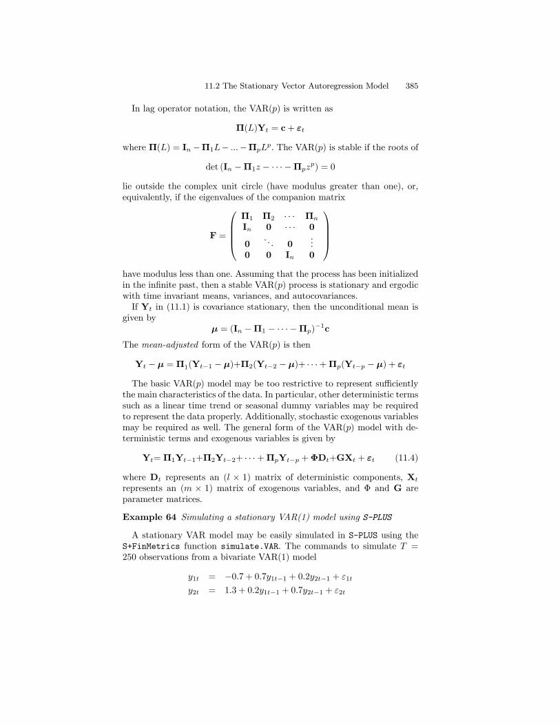
where the n.old optional argument specifies the number of observations toplot from uscn.ts. If n.old is not specified, all the observations in uscn.tswill be plotted together with uscn.pred. Figure 11.5 shows the forecastsproduced from the VAR(1) fit to the US/CN exchange rate data2. At thebeginning of the forecast horizon the spot return is below its estimatedmean value, and the forward premium is above its mean values. The spotreturn forecasts start off negative and grow slowly toward the mean, and theforward premium forecasts decline sharply toward the mean. The forecaststandard errors for both sets of forecasts, however, are fairly large.
2Notice that the dates associated with the forecasts are not shown. This is the resultof “timeDate” objects not having a well defined frequency from which to extrapolatedates.
400 11. Vector Autoregressive Models for Multivariate Time Series
-0.0
10.
00.
01
235 240 245 250 255
dspot
-0.0
02-0
.001
0.0
235 240 245 250 255
fp
index
valu
es
FIGURE 11.5. Predicted values from VAR(1) model fit to US/CN exchange ratedata.
11.3.2 Simulation-Based Forecasting
The previous subsection showed how to generate multivariate forecasts froma fitted VAR model, using the chain-rule of forecasting (11.8). Since themultivariate forecast errors (11.9) are asymptotically normally distributedwith covariance matrix (11.10), the forecasts of Yt+h can be simulatedby generating multivariate normal random variables with mean zero andcovariance matrix (11.10). These simulation-based forecasts can be ob-tained by setting the optional argument method to "mc" in the call topredict.VAR.When method="mc", the multivariate normal random variables are ac-
tually generated as a vector of standard normal random variables scaledby the Cholesky factor of the covariance matrix (11.10). Instead of usingstandard normal random variables, one could also use the standardizedresiduals from the fitted VAR model. Simulation-based forecasts based onthis approach are obtained by setting the optional argument method to"bootstrap" in the call to predict.VAR.
Example 67 Simulation-based forecasts of exchange rate data from bivari-ate VAR
The h-step forecasts (h = 1, . . . , 12) for∆st+h and fpt+h using the MonteCarlo simulation method are

11.3 Forecasting 401
> uscn.pred.MC = predict(var1.fit,n.predict=12,method="mc")
> summary(uscn.pred.MC)
Predicted Values with Standard Errors:
dspot fp
1-step-ahead -0.0032 -0.0005
(std.err) 0.0133 0.0009
2-step-ahead -0.0026 -0.0006
(std.err) 0.0133 0.0012
...
12-step-ahead -0.0013 -0.0013
(std.err) 0.0139 0.0015
TheMonte Carlo forecasts and forecast standard errors for fpt+h are almostidentical to those computed using the chain-rule of forecasting. The MonteCarlo forecasts for ∆st+h are slightly different and the forecast standarderrors are slightly larger than the corresponding values computed from thechain-rule.The h-step forecasts computed from the bootstrap simulation method
are
> uscn.pred.boot = predict(var1.fit,n.predict=12,
+ method="bootstrap")
> summary(uscn.pred.boot)
Predicted Values with Standard Errors:
dspot fp
1-step-ahead -0.0020 -0.0005
(std.err) 0.0138 0.0009
2-step-ahead -0.0023 -0.0007
(std.err) 0.0140 0.0012
...
12-step-ahead -0.0023 -0.0013
(std.err) 0.0145 0.0015
As with the Monte Carlo forecasts, the bootstrap forecasts and forecaststandard errors for fpt+h are almost identical to those computed using thechain-rule of forecasting. The bootstrap forecasts for ∆st+h are slightlydifferent from the chain-rule and Monte Carlo forecasts. In particular, thebootstrap forecast standard errors are larger than corresponding valuesfrom the chain-rule and Monte Carlo methods.The simulation-based forecasts described above are different from the
traditional simulation-based approach taken in VAR literature, e.g., see

402 11. Vector Autoregressive Models for Multivariate Time Series
Runkle (1987). The traditional approach is implemented using the followingprocedure:
1. Obtain VAR coefficient estimates Π and residuals εt.
2. Simulate the fitted VAR model by Monte Carlo simulation or bybootstrapping the fitted residuals εt.
3. Obtain new estimates of Π and forecasts of Yt+h based on the sim-ulated data.
The above procedure is repeated many times to obtain simulation-basedforecasts as well as their confidence intervals. To illustrate this approach,generate 12-step ahead forecasts from the fitted VAR object var1.fit byMonte Carlo simulation using the S+FinMetrics function simulate.VARas follows:
> set.seed(10)
> n.pred=12
> n.sim=100
> sim.pred = array(0,c(n.sim, n.pred, 2))
> y0 = seriesData(var1.fit$Y0)
> for (i in 1:n.sim) {
+ dat = simulate.VAR(var1.fit,n=243)
+ dat = rbind(y0,dat)
+ mod = VAR(dat~ar(1))
+ sim.pred[i,,] = predict(mod,n.pred)$values
+ }
The simulation-based forecasts are obtained by averaging the simulatedforecasts:
> colMeans(sim.pred)
[,1] [,2]
[1,] -0.0017917 -0.0012316
[2,] -0.0017546 -0.0012508
[3,] -0.0017035 -0.0012643
[4,] -0.0016800 -0.0012741
[5,] -0.0016587 -0.0012814
[6,] -0.0016441 -0.0012866
[7,] -0.0016332 -0.0012904
[8,] -0.0016253 -0.0012932
[9,] -0.0016195 -0.0012953
[10,] -0.0016153 -0.0012967
[11,] -0.0016122 -0.0012978
[12,] -0.0016099 -0.0012986

11.3 Forecasting 403
Comparing these forecasts with those in uscn.pred computed earlier, onecan see that for the first few forecasts, these simulated forecasts are slightlydifferent from the asymptotic forecasts. However, at larger steps, they ap-proach the long run stable values of the asymptotic forecasts.
Conditional Forecasting
The forecasts algorithms considered up to now are unconditional multivari-ate forecasts. However, sometimes it is desirable to obtain forecasts of somevariables in the system conditional on some knowledge of the future pathof other variables in the system. For example, when forecasting multivari-ate macroeconomic variables using quarterly data from a VAR model, itmay happen that some of the future values of certain variables in the VARmodel are known, because data on these variables are released earlier thandata on the other variables. By incorporating the knowledge of the futurepath of certain variables, in principle it should be possible to obtain morereliable forecasts of the other variables in the system. Another use of con-ditional forecasting is the generation of forecasts conditional on different“policy” scenarios. These scenario-based conditional forecasts allow one toanswer the question: if something happens to some variables in the systemin the future, how will it affect forecasts of other variables in the future?S+FinMetrics provides a generic function cpredict for computing con-
ditional forecasts, which has a method cpredict.VAR for “VAR” objects.The algorithms in cpredict.VAR are based on the conditional forecastingalgorithms described in Waggoner and Zha (1999). Waggoner and Zha clas-sify conditional information into “hard” conditions and “soft conditions”.The hard conditions restrict the future values of certain variables at fixedvalues, while the soft conditions restrict the future values of certain vari-ables in specified ranges. The arguments taken by cpredict.VAR are:
> args(cpredict.VAR)
function(object, n.predict = 1, newdata = NULL, olddata = NULL,
method = "mc", unbiased = T, variables.conditioned =
NULL, steps.conditioned = NULL, upper = NULL, lower =
NULL, middle = NULL, seed = 100, n.sim = 1000)
Like most predict methods in S-PLUS, the first argument must be a fittedmodel object, while the second argument, n.predict, specifies the numberof steps to predict ahead. The arguments newdata and olddata can usuallybe safely ignored, unless exogenous variables were used in fitting the model.With classical forecasts that ignore the uncertainty in coefficient esti-
mates, hard conditional forecasts can be obtained in closed form as shownby Doan, Litterman and Sims (1984), and Waggoner and Zha (1999). Toobtain hard conditional forecasts, the argument middle is used to specifyfixed values of certain variables at certain steps. For example, to fix the

404 11. Vector Autoregressive Models for Multivariate Time Series
1-step ahead forecast of dspot in var1.fit at -0.005 and generate otherpredictions for 2-step ahead forecasts, use the following command:
> cpredict(var1.fit, n.predict=2, middle=-0.005,
+ variables="dspot", steps=1)
Predicted Values:
dspot fp
1-step-ahead -0.0050 -0.0005
2-step-ahead -0.0023 -0.0007
In the call to cpredict, the optional argument variables is used to specifythe restricted variables, and steps to specify the restricted steps.To specify a soft condition, the optional arguments upper and lower
are used to specify the upper bound and lower bound, respectively, of asoft condition. Since closed form results are not available for soft condi-tional forecasts, either Monte Carlo simulation or bootstrap methods areused to obtain the actual forecasts. The simulations follow a similar proce-dure implemented in the function predict.VAR, except that a reject/acceptmethod to sample from the distribution conditional on the soft conditionsis used. For example, to restrict the range of the first 2-step ahead forecastsof dspot to be (−0.004,−0.001) use:
> cpredict(var1.fit, n.predict=2, lower=c(-0.004, -0.004),
+ upper=c(-0.001, -0.001), variables="dspot",
+ steps=c(1,2))
Predicted Values:
dspot fp
1-step-ahead -0.0027 -0.0003
2-step-ahead -0.0029 -0.0005
11.4 Structural Analysis
The general VAR(p) model has many parameters, and they may be difficultto interpret due to complex interactions and feedback between the variablesin the model. As a result, the dynamic properties of a VAR(p) are oftensummarized using various types of structural analysis. The three main typesof structural analysis summaries are (1) Granger causality tests; (2) impulseresponse functions; and (3) forecast error variance decompositions. Thefollowing sections give brief descriptions of these summary measures.

11.4 Structural Analysis 405
11.4.1 Granger Causality
One of the main uses of VAR models is forecasting. The structure of theVAR model provides information about a variable’s or a group of variables’forecasting ability for other variables. The following intuitive notion of avariable’s forecasting ability is due to Granger (1969). If a variable, orgroup of variables, y1 is found to be helpful for predicting another variable,or group of variables, y2 then y1 is said to Granger-cause y2; otherwise itis said to fail to Granger-cause y2. Formally, y1 fails to Granger-cause y2if for all s > 0 the MSE of a forecast of y2,t+s based on (y2,t, y2,t−1, . . .) isthe same as the MSE of a forecast of y2,t+s based on (y2,t, y2,t−1, . . .) and(y1,t, y1,t−1, . . .). Clearly, the notion of Granger causality does not implytrue causality. It only implies forecasting ability.
Bivariate VAR Models
In a bivariate VAR(p) model for Yt = (y1t, y2t)0, y2 fails to Granger-cause
y1 if all of the p VAR coefficient matrices Π1, . . . ,Πp are lower triangular.That is, the VAR(p) model has the formµ
y1ty2t
¶=
µc1c2
¶+
µπ111 0π121 π122
¶µy1t−1y2t−1
¶+ · · ·
+
µπp11 0πp21 πp22
¶µy1t−py2t−p
¶+
µε1tε2t
¶so that all of the coefficients on lagged values of y2 are zero in the equationfor y1. Similarly, y1 fails to Granger-cause y2 if all of the coefficients onlagged values of y1 are zero in the equation for y2. The p linear coefficientrestrictions implied by Granger non-causality may be tested using the Waldstatistic (11.5). Notice that if y2 fails to Granger-cause y1 and y1 failsto Granger-cause y2, then the VAR coefficient matrices Π1, . . . ,Πp arediagonal.
General VAR Models
Testing for Granger non-causality in general n variable VAR(p) modelsfollows the same logic used for bivariate models. For example, consider aVAR(p) model with n = 3 and Yt = (y1t, y2t, y3t)
0. In this model, y2 doesnot Granger-cause y1 if all of the coefficients on lagged values of y2 are zeroin the equation for y1. Similarly, y3 does not Granger-cause y1 if all of thecoefficients on lagged values of y3 are zero in the equation for y1. Thesesimple linear restrictions may be tested using the Wald statistic (11.5). Thereader is encouraged to consult Lutkepohl (1991) or Hamilton (1994) formore details and examples.
Example 68 Testing for Granger causality in bivariate VAR(2) model forexchange rates

406 11. Vector Autoregressive Models for Multivariate Time Series
Consider testing for Granger causality in a bivariate VAR(2) model forYt = (∆st, fpt)
0. Using the notation of (11.2), fpt does not Granger cause∆st if π
112 = 0 and π212 = 0. Similarly, ∆st does not Granger cause fpt if
π121 = 0 and π221 = 0. These hypotheses are easily tested using the Waldstatistic (11.5). The restriction matrix R for the hypothesis that fpt doesnot Granger cause ∆st is
R =
µ0 0 1 0 0 0 0 0 0 00 0 0 0 1 0 0 0 0 0
¶and the matrix for the hypothesis that ∆st does not Granger cause fpt is
R =
µ0 0 0 0 0 0 1 0 0 00 0 0 0 0 0 0 0 1 0
¶The S-PLUS commands to compute and evaluate these Granger causalityWald statistics are
> var2.fit = VAR(cbind(dspot,fp)~ar(2),data=uscn.ts)
> # H0: fp does not Granger cause dspot
> R = matrix(c(0,0,1,0,0,0,0,0,0,0,
+ 0,0,0,0,1,0,0,0,0,0),
+ 2,10,byrow=T)
> vecPi = as.vector(coef(var2.fit))
> avar = R%*%vcov(var2.fit)%*%t(R)
> wald = t(R%*%vecPi)%*%solve(avar)%*%(R%*%vecPi)
> wald
[,1]
[1,] 8.468844
> 1-pchisq(wald,2)
[1] 0.01448818
> R = matrix(c(0,0,0,0,0,0,1,0,0,0,
+ 0,0,0,0,0,0,0,0,1,0),
+ 2,10,byrow=T)
> vecPi = as.vector(coef(var2.fit))
> avar = R%*%vcov(var2.fit)%*%t(R)
> wald = t(R%*%vecPi)%*%solve(avar)%*%(R%*%vecPi)
> wald
[,1]
[1,] 6.157
> 1-pchisq(wald,2)
[1] 0.04604
The p-values for the Wald tests indicate a fairly strong rejection of the nullthat fpt does not Granger cause ∆st but only a weak rejection of the nullthat ∆st does not Granger cause fpt. Hence, lagged values of fpt appear

11.4 Structural Analysis 407
to be useful for forecasting future values of ∆st and lagged values of ∆stappear to be useful for forecasting future values of fpt.
11.4.2 Impulse Response Functions
Any covariance stationary VAR(p) process has a Wold representation ofthe form
Yt= µ+ εt+Ψ1εt−1+Ψ2εt−2 + · · · (11.11)
where the (n× n) moving average matrices Ψs are determined recursivelyusing (11.6). It is tempting to interpret the (i, j)-th element, ψsij , of thematrix Ψs as the dynamic multiplier or impulse response
∂yi,t+s∂εj,t
=∂yi,t∂εj,t−s
= ψsij , i, j = 1, . . . , n
However, this interpretation is only possible if var(εt) = Σ is a diagonalmatrix so that the elements of εt are uncorrelated. One way to make theerrors uncorrelated is to follow Sims (1980) and estimate the triangularstructural VAR(p) model
y1t = c1 + γ011Yt−1+ · · ·+ γ01pYt−p + η1t (11.12)
y2t = c1 + β21y1t+γ021Yt−1+ · · ·+ γ02pYt−p + η2t
y3t = c1 + β31y1t + β32y2t+γ031Yt−1+ · · ·+ γ03pYt−p + η3t
...
ynt = c1 + βn1y1t + · · ·+ βn,n−1yn−1,t + γ0n1Yt−1+ · · ·+ γ0npYt−p + ηnt
In matrix form, the triangular structural VAR(p) model is
BYt= c+ Γ1Yt−1+Γ2Yt−2+ · · ·+ ΓpYt−p + ηt (11.13)
where
B =
1 0 · · · 0−β21 1 0 0...
.... . .
...−βn1 −βn2 · · · 1
(11.14)
is a lower triangular matrix with 10s along the diagonal. The algebra ofleast squares will ensure that the estimated covariance matrix of the errorvector ηt is diagonal. The uncorrelated/orthogonal errors ηt are referredto as structural errors.The triangular structural model (11.12) imposes the recursive causal or-
dering
y1 → y2 → · · ·→ yn (11.15)

408 11. Vector Autoregressive Models for Multivariate Time Series
The ordering (11.15) means that the contemporaneous values of the vari-ables to the left of the arrow → affect the contemporaneous values of thevariables to the right of the arrow but not vice-versa. These contempora-neous effects are captured by the coefficients βij in (11.12). For example,the ordering y1 → y2 → y3 imposes the restrictions: y1t affects y2t and y3tbut y2t and y3t do not affect y1; y2t affects y3t but y3t does not affect y2t.Similarly, the ordering y2 → y3 → y1 imposes the restrictions: y2t affectsy3t and y1t but y3t and y1t do not affect y2; y3t affects y1t but y1t does notaffect y3t. For a VAR(p) with n variables there are n! possible recursivecausal orderings. Which ordering to use in practice depends on the contextand whether prior theory can be used to justify a particular ordering. Re-sults from alternative orderings can always be compared to determine thesensitivity of results to the imposed ordering.Once a recursive ordering has been established, the Wold representation
of Yt based on the orthogonal errors ηt is given by
Yt= µ+Θ0ηt+Θ1ηt−1+Θ2ηt−2 + · · · (11.16)
where Θ0 = B−1 is a lower triangular matrix. The impulse responses tothe orthogonal shocks ηjt are
∂yi,t+s∂ηj,t
=∂yi,t∂ηj,t−s
= θsij , i, j = 1, . . . , n; s > 0 (11.17)
where θsij is the (i, j) th element of Θs. A plot of θsij against s is called the
orthogonal impulse response function (IRF) of yi with respect to ηj . Withn variables there are n2 possible impulse response functions.In practice, the orthogonal IRF (11.17) based on the triangular VAR(p)
(11.12) may be computed directly from the parameters of the non triangularVAR(p) (11.1) as follows. First, decompose the residual covariance matrixΣ as
Σ = ADA0
whereA is an invertible lower triangular matrix with 10s along the diagonaland D is a diagonal matrix with positive diagonal elements. Next, definethe structural errors as
ηt= A−1εt
These structural errors are orthogonal by construction since var(ηt) =A−1ΣA−10= A−1ADA0A−10= D. Finally, re-express the Wold represen-tation (11.11) as
Yt = µ+AA−1εt+Ψ1AA−1εt−1+Ψ2AA−1εt−2 + · · ·= µ+Θ0ηt +Θ1ηt−1+Θ2ηt−2 + · · ·
where Θj= ΨjA. Notice that the structural B matrix in (11.13) is equalto A−1.

11.4 Structural Analysis 409
Computing the Orthogonal Impulse Response Function Using theS+FinMetrics Function impRes
The orthogonal impulse response function (11.17) from a triangular struc-tural VAR model (11.13) may be computed using the S+FinMetrics func-tion impRes. The function impRes has arguments
> args(impRes)
function(x, period = NULL, std.err = "none", plot = F,
unbiased = T, order = NULL, ...)
where x is an object of class “VAR” and period specifies the number ofresponses to compute. By default, no standard errors for the responsesare computed. To compute asymptotic standard errors for the responses,specify std.err="asymptotic". To create a panel plot of all the responsefunctions, specify plot=T. The default recursive causal ordering is based onthe ordering of the variables in Yt when the VAR model is fit. The optionalargument order may be used to specify a different recursive causal order-ing for the computation of the impulse responses. The argument order ac-cepts a character vector of variable names whose order defines the recursivecausal ordering. The output of impRes is an object of class “impDecomp” forwhich there are print, summary and plot methods. The following exampleillustrates the use of impRes.
Example 69 IRF from VAR(1) for exchange rates
Consider again the VAR(1) model for Yt = (∆st, fpt)0. For the impulse
response analysis, the initial ordering of the variables imposes the assump-tion that structural shocks to fpt have no contemporaneous effect on ∆stbut structural shocks to ∆st do have a contemporaneous effect on fpt. Tocompute the four impulse response functions
∂∆st+h∂η1t
,∂∆st+h∂η2t
,∂fpt+h∂η1t
,∂fpt+h∂η2t
for h = 1, . . . , 12 we use S+FinMetrics function impRes. The first twelveimpulse responses from the VAR(1) model for exchange rates are computedusing
> uscn.irf = impRes(var1.fit, period=12, std.err="asymptotic")
The print method shows the impulse response values without standarderrors:
> uscn.irf
Impulse Response Function:
(with responses in rows, and innovations in columns)

410 11. Vector Autoregressive Models for Multivariate Time Series
, , lag.0
dspot fp
dspot 0.0136 0.0000
fp 0.0000 0.0009
, , lag.1
dspot fp
dspot -0.0018 -0.0013
fp 0.0001 0.0007
, , lag.2
dspot fp
dspot 0.0000 -0.0009
fp 0.0001 0.0006
...
, , lag.11
dspot fp
dspot 0.0000 -0.0001
fp 0.0000 0.0001
The summary method will display the responses with standard errors andt-statistics. The plot method will produce a four panel Trellis graphicsplot of the impulse responses
> plot(uscn.irf)
A plot of the impulse responses can also be created in the initial call toimpRes by using the optional argument plot=T.Figure 11.6 shows the impulse response functions along with asymptotic
standard errors. The top row shows the responses of ∆st to the structuralshocks, and the bottom row shows the responses of fpt to the structuralshocks. In response to the first structural shock, η1t, ∆st initially increasesbut then drops quickly to zero after 2 months. Similarly, fpt initially in-creases, reaches its peak response in 2 months and then gradually dropsoff to zero after about a year. In response to the second shock, η2t, byassumption ∆st has no initial response. At one month, a sharp drop occursin ∆st followed by a gradual return to zero after about a year. In contrast,fpt initially increases and then gradually drops to zero after about a year.The orthogonal impulse responses in Figure 11.6 are based on the recur-
sive causal ordering ∆st → fpt. It must always be kept in mind that thisordering identifies the orthogonal structural shocks η1t and η2t. If the or-dering is reversed, then a different set of structural shocks will be identified,and these may give very different impulse response functions. To compute

11.4 Structural Analysis 411
0.0
0.00
010
0.00
020
0 2 4 6 8 10
Inno.: dspotResp.: fp
0.0
0.00
040.
0008
Inno.: fpResp.: fp
0.0
0.00
50.
010
Inno.: dspotResp.: dspot
-0.0
015
-0.0
005
0.0
0 2 4 6 8 10
Inno.: fpResp.: dspot
Steps
Impu
lse
Res
pons
e
Orthogonal Impulse Response Function
FIGURE 11.6. Impulse response function from VAR(1) model fit to US/CN ex-change rate data with ∆st ordered first.
the orthogonal impulse responses using the alternative ordering fpt → ∆stspecify order=c("fp","dspot") in the call to impRes:
> uscn.irf2 = impRes(var1.fit,period=12,std.err="asymptotic",
+ order=c("fp","dspot"),plot=T)
These impulse responses are presented in Figure 11.7 and are almost iden-tical to those computed using the ordering ∆st → fpt. The reason for thisresponse is that the reduced form VAR residuals ε1t and ε2t are almostuncorrelated. To see this, the residual correlation matrix may be computedusing
> sd.vals = sqrt(diag(var1.fit$Sigma))
> cor.mat = var1.fit$Sigma/outer(sd.vals,sd.vals)
> cor.mat
dspot fp
dspot 1.000000 0.033048
fp 0.033048 1.000000
Because of the near orthogonality in the reduced form VAR errors, theerror in the ∆st equation may be interpreted as an orthogonal shock to theexchange rate and the error in the fpt equation may be interpreted as anorthogonal shock to the forward premium.

412 11. Vector Autoregressive Models for Multivariate Time Series
-0.0
020
-0.0
005
0.00
10
0 2 4 6 8 10
Inno.: fpResp.: dspot
0.0
0.00
50.
010
Inno.: dspotResp.: dspot0.
00.
0004
0.00
08
Inno.: fpResp.: fp
0.0
0.00
005
0.00
015
0 2 4 6 8 10
Inno.: dspotResp.: fp
Steps
Impu
lse
Res
pons
e
Orthogonal Impulse Response Function
FIGURE 11.7. Impulse response function from VAR(1) model fit to US/CN ex-change rate with fpt ordered first.
11.4.3 Forecast Error Variance Decompositions
The forecast error variance decomposition (FEVD) answers the question:what portion of the variance of the forecast error in predicting yi,T+h isdue to the structural shock ηj? Using the orthogonal shocks ηt the h-stepahead forecast error vector, with known VAR coefficients, may be expressedas
YT+h −YT+h|T =h−1Xs=0
ΘsηT+h−s
For a particular variable yi,T+h, this forecast error has the form
yi,T+h − yi,T+h|T =h−1Xs=0
θsi1η1,T+h−s + · · ·+h−1Xs=0
θsinηn,T+h−s
Since the structural errors are orthogonal, the variance of the h-step fore-cast error is
var(yi,T+h − yi,T+h|T ) = σ2η1
h−1Xs=0
(θsi1)2+ · · ·+ σ2ηn
h−1Xs=0
(θsin)2

11.4 Structural Analysis 413
where σ2ηj = var(ηjt). The portion of var(yi,T+h − yi,T+h|T ) due to shockηj is then
FEVDi,j(h) =σ2ηj
Ph−1s=0
¡θsij¢2
σ2η1Ph−1
s=0 (θsi1)
2 + · · ·+ σ2ηnPh−1
s=0 (θsin)
2, i, j = 1, . . . , n
(11.18)In a VAR with n variables there will be n2 FEVDi,j(h) values. It must bekept in mind that the FEVD in (11.18) depends on the recursive causal or-dering used to identify the structural shocks ηt and is not unique. Differentcausal orderings will produce different FEVD values.
Computing the FEVD Using the S+FinMetrics Function fevDec
Once a VAR model has been fit, the S+FinMetrics function fevDec maybe used to compute the orthogonal FEVD. The function fevDec has argu-ments
> args(fevDec)
function(x, period = NULL, std.err = "none", plot = F,
unbiased = F, order = NULL, ...)
where x is an object of class “VAR” and period specifies the number ofresponses to compute. By default, no standard errors for the responsesare computed and no plot is created. To compute asymptotic standarderrors for the responses, specify std.err="asymptotic" and to plot thedecompositions, specify plot=T. The default recursive causal ordering isbased on the ordering of the variables inYt when the VAR model is fit. Theoptional argument ordermay be used to specify a different recursive causalordering for the computation of the FEVD. The argument order acceptsa text string vector of variable names whose order defines the recursivecausal ordering. The output of fevDec is an object of class “impDecomp”for which there are print, summary and plot methods. The use of fevDecis illustrated with the following example.
Example 70 FEVD from VAR(1) for exchange rates
The orthogonal FEVD of the forecast errors from the VAR(1) modelfit to the US/CN exchange rate data using the recursive causal ordering∆st → fpt is computed using
> uscn.fevd = fevDec(var1.fit,period=12,
+ std.err="asymptotic")
> uscn.fevd
Forecast Error Variance Decomposition:
(with responses in rows, and innovations in columns)

414 11. Vector Autoregressive Models for Multivariate Time Series
, , 1-step-ahead
dspot fp
dspot 1.0000 0.0000
fp 0.0011 0.9989
, , 2-step-ahead
dspot fp
dspot 0.9907 0.0093
fp 0.0136 0.9864
...
, , 12-step-ahead
dspot fp
dspot 0.9800 0.0200
fp 0.0184 0.9816
The summary method adds standard errors to the above output if they arecomputed in the call to fevDec. The plot method produces a four panelTrellis graphics plot of the decompositions:
> plot(uscn.fevd)
The FEVDs in Figure 11.8 show that most of the variance of the forecasterrors for ∆st+s at all horizons s is due to the orthogonal ∆st innovations.Similarly, most of the variance of the forecast errors for fpt+s is due to theorthogonal fpt innovations.The FEVDs using the alternative recursive causal ordering fpt → ∆st
are computed using
> uscn.fevd2 = fevDec(var1.fit,period=12,
+ std.err="asymptotic",order=c("fp","dspot"),plot=T)
and are illustrated in Figure 11.9. Since the residual covariance matrix isalmost diagonal (see analysis of IRF above), the FEVDs computed usingthe alternative ordering are almost identical to those computed with theinitial ordering.
11.5 An Extended Example
In this example the causal relations and dynamic interactions among monthlyreal stock returns, real interest rates, real industrial production growth andthe inflation rate is investigated using a VAR model. The analysis is similarto that of Lee (1992). The variables are in the S+FinMetrics “timeSeries”object varex.ts
> colIds(varex.ts)

11.5 An Extended Example 415
0.0
0.01
0.02
0.03
0.04
2 4 6 8 10 12
Inno.: dspotResp.: fp
0.96
0.97
0.98
0.99
1.00
Inno.: fpResp.: fp
0.97
0.98
0.99
1.00
Inno.: dspotResp.: dspot
0.0
0.01
0.02
0.03
2 4 6 8 10 12
Inno.: fpResp.: dspot
Forecast Steps
Prop
ortio
n of
Var
ianc
e C
ontri
butio
n
Forecast Error Variance Decomposition
FIGURE 11.8. Orthogonal FEVDs computed from VAR(1) model fit to US/CNexchange rate data using the recursive causal ordering with ∆st first.
[1] "MARKET.REAL" "RF.REAL" "INF" "IPG"
Details about the data are in the documentation slot of varex.ts
> varex.ts@documentation
To be comparable to the results in Lee (1992), the analysis is conductedover the postwar period January 1947 through December 1987
> smpl = (positions(varex.ts) >= timeDate("1/1/1947") &
+ positions(varex.ts) < timeDate("1/1/1988"))
The data over this period is displayed in Figure 11.10. All variables appearto be I(0), but the real T-bill rate and the inflation rate appear to be highlypersistent.To begin the analysis, autocorrelations and cross correlations at leads
and lags are computed using
> varex.acf = acf(varex.ts[smpl,])
and are illustrated in Figure 11.11. The real return on the market shows asignificant positive first lag autocorrelation, and inflation appears to leadthe real market return with a negative sign. The real T-bill rate is highlypositively autocorrelated, and inflation appears to lead the real T-bill ratestrongly with a negative sign. Inflation is also highly positively autocorre-lated and, interestingly, the real T-bill rate appears to lead inflation with

416 11. Vector Autoregressive Models for Multivariate Time Series
0.0
0.01
0.02
0.03
0.04
2 4 6 8 10 12
Inno.: fpResp.: dspot
0.96
0.97
0.98
0.99
1.00
Inno.: dspotResp.: dspot0.
975
0.98
50.
995
Inno.: fpResp.: fp
0.0
0.01
00.
020
2 4 6 8 10 12
Inno.: dspotResp.: fp
Forecast Steps
Prop
ortio
n of
Var
ianc
e C
ontri
butio
n
Forecast Error Variance Decomposition
FIGURE 11.9. Orthogonal FEVDs from VAR(1) model fit to US/CN exchangerate data using recursive causal ordering with fpt first.
a positive sign. Finally, industrial production growth is slightly positivelyautocorrelated, and the real market return appears to lead industrial pro-duction growth with a positive sign.The VAR(p) model is fit with the lag length selected by minimizing the
AIC and a maximum lag length of 6 months:
> varAIC.fit = VAR(varex.ts,max.ar=6,criterion="AIC",
+ start="Jan 1947",end="Dec 1987",
+ in.format="%m %Y")
The lag length selected by minimizing AIC is p = 2:
> varAIC.fit$info
ar(1) ar(2) ar(3) ar(4) ar(5) ar(6)
AIC -14832 -14863 -14853 -14861 -14855 -14862
> varAIC.fit$ar.order
[1] 2
The results of the VAR(2) fit are
> summary(varAIC.out)
Call:
VAR(data = varex.ts, start = "Jan 1947", end = "Dec 1987",

11.5 An Extended Example 417
Real Return on Market
1930 1950 1970 1990
-0.3
-0.1
0.1
0.3
Real Interest Rate
1930 1950 1970 1990
-0.0
15-0
.005
0.00
5
Industrial Production Growth
1930 1950 1970 1990
-0.1
00.
000.
10
Inflation
1930 1950 1970 1990
-0.0
20.
020.
05
FIGURE 11.10. Monthly data on stock returns, interest rates, output growth andinflation.
max.ar = 6, criterion = "AIC", in.format = "%m %Y")
Coefficients:
MARKET.REAL RF.REAL INF IPG
(Intercept) 0.0074 0.0002 0.0010 0.0019
(std.err) 0.0023 0.0001 0.0002 0.0007
(t.stat) 3.1490 4.6400 4.6669 2.5819
MARKET.REAL.lag1 0.2450 0.0001 0.0072 0.0280
(std.err) 0.0470 0.0011 0.0042 0.0146
(t.stat) 5.2082 0.0483 1.7092 1.9148
RF.REAL.lag1 0.8146 0.8790 0.5538 0.3772
(std.err) 2.0648 0.0470 0.1854 0.6419
(t.stat) 0.3945 18.6861 2.9867 0.5877
INF.lag1 -1.5020 -0.0710 0.4616 -0.0722
(std.err) 0.4932 0.0112 0.0443 0.1533
(t.stat) -3.0451 -6.3147 10.4227 -0.4710
MARKET.REAL RF.REAL INF IPG
IPG.lag1 -0.0003 0.0031 -0.0143 0.3454

418 11. Vector Autoregressive Models for Multivariate Time Series
MARKET.REAL
ACF
0 5 10 15 20
0.0
0.2
0.4
0.6
0.8
1.0
MARKET.REAL and RF.REAL
0 5 10 15 20
-0.0
50.
00.
05
MARKET.REAL and INF
0 5 10 15 20
-0.2
0-0
.15
-0.1
0-0
.05
0.0
0.05
0.10 MARKET.REAL and IPG
0 5 10 15 20
-0.1
5-0
.10
-0.0
50.
00.
05
RF.REAL and MARKET.REAL
ACF
-20 -15 -10 -5 0
-0.0
50.
00.
050.
10
RF.REAL
0 5 10 15 20
0.0
0.2
0.4
0.6
0.8
1.0
RF.REAL and INF
0 5 10 15 20
-0.3
-0.2
-0.1
0.0
0.1 RF.REAL and IPG
0 5 10 15 20
-0.0
50.
00.
050.
10
INF and MARKET.REAL
ACF
-20 -15 -10 -5 0
-0.1
5-0
.10
-0.0
50.
00.
05
INF and RF.REAL
-20 -15 -10 -5 0
-0.1
5-0
.10
-0.0
50.
00.
050.
10
INF
0 5 10 15 20
0.0
0.2
0.4
0.6
0.8
1.0
INF and IPG
0 5 10 15 20
-0.0
50.
00.
05
IPG and MARKET.REAL
Lag
ACF
-20 -15 -10 -5 0-0.1
0-0
.05
0.0
0.05
0.10
0.15
0.20
IPG and RF.REAL
Lag-20 -15 -10 -5 0
-0.0
50.
00.
05
IPG and INF
Lag-20 -15 -10 -5 0
-0.2
0-0
.15
-0.1
0-0
.05
0.0
0.05
IPG
Lag0 5 10 15 20
-0.2
0.0
0.2
0.4
0.6
0.8
1.0
FIGURE 11.11. Autocorrelations and cross correlations at leads and lags of datain VAR model.
(std.err) 0.1452 0.0033 0.0130 0.0452
(t.stat) -0.0018 0.9252 -1.0993 7.6501
MARKET.REAL.lag2 -0.0500 0.0022 -0.0066 0.0395
(std.err) 0.0466 0.0011 0.0042 0.0145
(t.stat) -1.0727 2.0592 -1.5816 2.7276
RF.REAL.lag2 -0.3481 0.0393 -0.5855 -0.3289
(std.err) 1.9845 0.0452 0.1782 0.6169
(t.stat) -0.1754 0.8699 -3.2859 -0.5331
INF.lag2 -0.0602 0.0079 0.2476 -0.0370
(std.err) 0.5305 0.0121 0.0476 0.1649
(t.stat) -0.1135 0.6517 5.1964 -0.2245
MARKET.REAL RF.REAL INF IPG
IPG.lag2 -0.1919 0.0028 0.0154 0.0941
(std.err) 0.1443 0.0033 0.0130 0.0449
(t.stat) -1.3297 0.8432 1.1868 2.0968
Regression Diagnostics:
MARKET.REAL RF.REAL INF IPG

11.5 An Extended Example 419
R-squared 0.1031 0.9299 0.4109 0.2037
Adj. R-squared 0.0882 0.9287 0.4011 0.1905
Resid. Scale 0.0334 0.0008 0.0030 0.0104
Information Criteria:
logL AIC BIC HQ
7503 -14935 -14784 -14875
total residual
Degree of freedom: 489 480
Time period: from Mar 1947 to Nov 1987
The signs of the statistically significant coefficient estimates corroboratethe informal analysis of the multivariate autocorrelations and cross lag au-tocorrelations. In particular, the real market return is positively related toits own lag but negatively related to the first lag of inflation. The real T-billrate is positively related to its own lag, negatively related to the first lag ofinflation, and positively related to the first lag of the real market return. In-dustrial production growth is positively related to its own lag and positivelyrelated to the first two lags of the real market return. Judging from thecoefficients it appears that inflation Granger causes the real market returnand the real T-bill rate, the real T-bill rate Granger causes inflation, andthe real market return Granger causes the real T-bill rate and industrialproduction growth. These observations are confirmed with formal tests forGranger non-causality. For example, the Wald statistic for testing the nullhypothesis that the real market return does not Granger-cause industrialproduction growth is
> bigR = matrix(0,2,36)
> bigR[1,29]=bigR[2,33]=1
> vecPi = as.vector(coef(varAIC.fit))
> avar = bigR%*%vcov(varAIC.fit)%*%t(bigR)
> wald = t(bigR%*%vecPi)%*%solve(avar)%*%(bigR%*%vecPi)
> as.numeric(wald)
[1] 13.82
> 1-pchisq(wald,2)
[1] 0.0009969
The 24-period IRF using the recursive causal ordering MARKET.REAL →RF.REAL → IPG → INF is computed using
> varAIC.irf = impRes(varAIC.fit,period=24,
+ order=c("MARKET.REAL","RF.REAL","IPG","INF"),
+ std.err="asymptotic",plot=T)
and is illustrated in Figure 11.12. The responses of MARKET.REAL to unex-pected orthogonal shocks to the other variables are given in the first row of

420 11. Vector Autoregressive Models for Multivariate Time Series
-0.0
003
0.0
0.00
02
0 5 10 15 20
Inno.: MARKET.REALResp.: INF
0.0
0.00
04
Inno.: RF.REALResp.: INF
-0.0
002
0.0
0.00
02
0 5 10 15 20
Inno.: IPGResp.: INF
0.0
0.00
150.
0030 Inno.: INF
Resp.: INF
0.0
0.00
100.
0025 Inno.: MARKET.REAL
Resp.: IPG
-0.0
002
0.00
04
Inno.: RF.REALResp.: IPG
0.0
0.00
40.
008
Inno.: IPGResp.: IPG
-0.0
010
-0.0
004
0.00
02 Inno.: INFResp.: IPG-1
.5*1
0^-4
0
Inno.: MARKET.REALResp.: RF.REAL
0.00
020.
0006
Inno.: RF.REALResp.: RF.REAL
-2*1
0^-5
6*10
^-5
Inno.: IPGResp.: RF.REAL
-0.0
004
-0.0
001
Inno.: INFResp.: RF.REAL
0.0
0.01
0.03
Inno.: MARKET.REALResp.: MARKET.REAL
-0.0
015
0.0
0.00
15
0 5 10 15 20
Inno.: RF.REALResp.: MARKET.REAL
-0.0
03-0
.001
0.00
1 Inno.: IPGResp.: MARKET.REAL
-0.0
06-0
.003
0.0
0 5 10 15 20
Inno.: INFResp.: MARKET.REAL
Steps
Impu
lse
Res
pons
e
Orthogonal Impulse Response Function
FIGURE 11.12. IRF using the recursive causal ordering MARKET.REAL→ RF.REAL
→ IPG → INF.
the figure. Most notable is the strong negative response of MARKET.REAL toan unexpected increase in inflation. Notice that it takes about ten monthsfor the effect of the shock to dissipate. The responses of RF.REAL to theorthogonal shocks is given in the second row of the figure. RF.REAL alsoreacts negatively to an inflation shock and the effect of the shock is felt forabout two years. The responses of IPG to the orthogonal shocks is givenin the third row of the figure. Industrial production growth responds posi-tively to an unexpected shock to MARKET.REAL and negatively to shocks toRF.REAL and INF. These effects, however, are generally short term. Finally,the fourth row gives the responses of INF to the orthogonal shocks. Infla-tion responds positively to a shock to the real T-bill rate, but this effect isshort-lived.The 24 month FEVD computed using the recursive causal ordering as
specified by MARKET.REAL → RF.REAL → IPG → INF,
> varAIC.fevd = fevDec(varAIC.out,period=24,
> order=c("MARKET.REAL","RF.REAL","IPG","INF"),
> std.err="asymptotic",plot=T)

11.5 An Extended Example 421
-0.0
020.
004
0.00
8
5 10 15 20
Inno.: MARKET.REALResp.: INF
0.01
0.03
0.05
Inno.: RF.REALResp.: INF
-0.0
020.
004
0.01
0
5 10 15 20
Inno.: IPGResp.: INF
0.94
0.98
Inno.: INFResp.: INF
0.0
0.04
Inno.: MARKET.REALResp.: IPG
-0.0
020.
004
0.00
8 Inno.: RF.REALResp.: IPG
0.90
0.94
0.98
Inno.: IPGResp.: IPG
0.0
0.01
00.
025
Inno.: INFResp.: IPG
0.01
0.03
Inno.: MARKET.REALResp.: RF.REAL
0.5
0.7
0.9
Inno.: RF.REALResp.: RF.REAL
-0.0
050.
005
0.01
5
Inno.: IPGResp.: RF.REAL
0.0
0.2
0.4
Inno.: INFResp.: RF.REAL
0.94
0.98
Inno.: MARKET.REALResp.: MARKET.REAL
-0.0
005
0.00
10
5 10 15 20
Inno.: RF.REALResp.: MARKET.REAL
-0.0
020.
004
0.01
0
Inno.: IPGResp.: MARKET.REAL
0.0
0.02
0.04
0.06
5 10 15 20
Inno.: INFResp.: MARKET.REAL
Forecast Steps
Prop
ortio
n of
Var
ianc
e C
ontri
butio
n
Forecast Error Variance Decomposition
FIGURE 11.13. FEVDs using the recursive causal ordering MARKET.REAL →RF.REAL → IPG → INF.
is illustrated in Figure 11.13. The first row gives the variance decom-positions for MARKET.REAL and shows that most of the variance of theforecast errors is due to own shocks. The second row gives the decomposi-tions for RF.REAL. At short horizons, most of the variance is attributableto own shocks but at long horizons inflation shocks account for almosthalf the variance. The third row gives the variance decompositions for IPG.Most of the variance is due to own shocks and a small fraction is due toMARKET.REAL shocks. Finally, the fourth row shows that the forecast errorvariance of INF is due mostly to its own shocks.The IRFs and FEVDs computed above depend on the imposed recursive
causal ordering. However, in this example, the ordering of the variables willhave little effect on the IRFs and FEVDs because the errors in the reducedform VAR are nearly uncorrelated:
> sd.vals = sqrt(diag(varAIC.out$Sigma))
> cor.mat = varAIC.out$Sigma/outer(sd.vals,sd.vals)
> cor.mat
MARKET.REAL RF.REAL INF IPG
MARKET.REAL 1.00000 -0.16855 -0.04518 0.03916
RF.REAL -0.16855 1.00000 0.13046 0.03318
INF -0.04518 0.13046 1.00000 0.04732
IPG 0.03916 0.03318 0.04732 1.00000

422 11. Vector Autoregressive Models for Multivariate Time Series
11.6 Bayesian Vector Autoregression
VAR models with many variables and long lags contain many parameters.Unrestricted estimation of these models reqires lots of data and often theestimated parameters are not very precise, the results are hard to inter-pret, and forecasts may appear more precise than they really are becausestandard error bands do not account for parameter uncertainty. The esti-mates and forecasts can be improved if one has prior information aboutthe structure of the model or the possible values of the parameters or func-tions of the parameters. In a classical framework, it is difficult to incorpo-rate non-sample information into the estimation. Nonsample informationis easy to incorporate in a Bayesian framework. A Bayesian frameworkalso naturally incorporates parameter uncertainty into common measuresof precision. This section briefly describes the Bayesian VAR modelingtools in S+FinMetrics and illustrates these tools with an example. Detailsof underlying Bayesian methods are given in Sims and Zha (1998) and Zha(1998).
11.6.1 An Example of a Bayesian VAR Model
S+FinMetrics comes with a “timeSeries” object policy.dat, which con-tains six U.S. macroeconomic variables:
> colIds(policy.dat)
[1] "CP" "M2" "FFR" "GDP" "CPI" "U"
which represent IMF’s index of world commodity prices, M2 money stock,federal funds rate, real GDP, consumer price index for urban consumers,and civilian unemployment rate. The data set contains monthly observa-tions from January 1959 to March 1998. Tao Zha and his co-authors haveanalyzed this data set in a number of papers, for example see Zha (1998).To use the same time period as in Zha (1998), create a subset of the data:
> zpolicy.dat = policy.dat[1:264,]
> zpolicy.mat = as.matrix(seriesData(zpolicy.dat))
which contains monthly observations from January 1959 to December1980.
Estimating a Bayesian VAR Model
To estimate a Bayesian vector autoregression model, use the S+FinMetricsfunction BVAR. For macroeconomic modeling, it is usually found that manytrending macroeconomic variables have a unit root, and in some cases,they may also have a cointegrating relationship (as described in the nextchapter). To incorporate these types of prior beliefs into the model, usethe unit.root.dummy and coint.dummy optional arguments to the BVAR

11.6 Bayesian Vector Autoregression 423
function, which add some dummy observations to the beginning of the datato reflect these beliefs:
> zpolicy.bar13 = BVAR(zpolicy.mat~ar(13), unit.root=T,
+ coint=T)
> class(zpolicy.bar13)
[1] "BVAR"
The returned object is of class “BVAR”, which inherits from “VAR”, so manymethod functions for “VAR” objects work similarly for “BVAR” objects, suchas the extractor functions, impulse response functions, and forecast errorvariance decomposition functions.The Bayesian VAR models are controlled through a set of hyper param-
eters, which can be specified using the optional argument control, whichis usually a list returned by the function BVAR.control. For example, thetightness of the belief in the unit root prior and cointegration prior is spec-ified by mu5 and mu6, respectively. To see what default values are used forthese hyper parameters, use
> args(BVAR.control)
function(L0 = 0.9, L1 = 0.1, L2 = 1, L3 = 1, L4 = 0.05,
mu5 = 5, mu6 = 5)
For the meanings of these hyper parameters, see the online help file forBVAR.control.
Adding Exogenous Variables to the Model
Other exogenous variables can be added to the estimation formula, justas for OLS and VAR functions. The BVAR function and related functionswill automatically take that into consideration and return the coefficientestimates for those variables.
Unconditional Forecasts
To forecast from a fitted Bayesian VAR model, use the generic predictfunction, which automatically calls the method function predict.BVAR foran object inheriting from class “BVAR”. For example, to compute 12-stepahead forecasts use
> zpolicy.bpred = predict(zpolicy.bar13,n.predict=12)
> class(zpolicy.bpred)
[1] "forecast"
> names(zpolicy.bpred)
[1] "values" "std.err" "draws"
> zpolicy.bpred
Predicted Values:

424 11. Vector Autoregressive Models for Multivariate Time Series
4.5
4.6
4.7
4.8 CP
4.3
4.4
4.5
4.6
245 250 255 260 265 270 275
CPI
0.10
0.12
0.14
0.16
0.18
0.20
FFR
8.42
8.43
8.44
8.45
8.46
8.47
245 250 255 260 265 270 275
GDP
7.25
7.30
7.35
7.40
7.45
M2
0.06
0.07
0.08
0.09
0.10
245 250 255 260 265 270 275
U
index
valu
es
FIGURE 11.14. Forecasts from Bayesian VAR model.
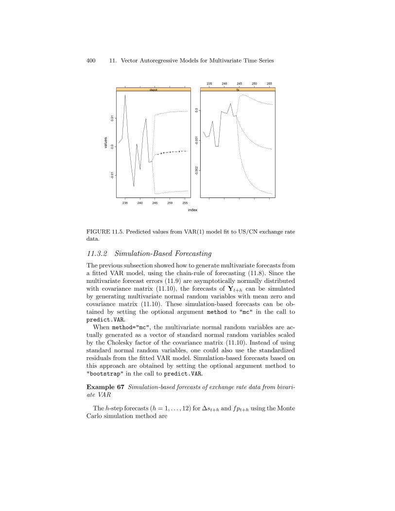
CP M2 FFR GDP CPI U
1-step-ahead 4.6354 7.3794 0.1964 8.4561 4.4714 0.0725
2-step-ahead 4.6257 7.3808 0.1930 8.4546 4.4842 0.0732
3-step-ahead 4.6247 7.3834 0.1823 8.4505 4.4960 0.0746
4-step-ahead 4.6310 7.3876 0.1670 8.4458 4.5065 0.0763
5-step-ahead 4.6409 7.3931 0.1515 8.4414 4.5160 0.0785
6-step-ahead 4.6503 7.3998 0.1384 8.4394 4.5244 0.0810
7-step-ahead 4.6561 7.4075 0.1309 8.4390 4.5321 0.0833
8-step-ahead 4.6552 7.4159 0.1307 8.4403 4.5397 0.0852
9-step-ahead 4.6496 7.4242 0.1362 8.4428 4.5475 0.0867
10-step-ahead 4.6415 7.4323 0.1451 8.4453 4.5561 0.0879
11-step-ahead 4.6321 7.4402 0.1546 8.4473 4.5655 0.0889
12-step-ahead 4.6232 7.4476 0.1618 8.4482 4.5753 0.0899
The forecasts can also be plotted along with the original data using
> plot(zpolicy.bpred, zpolicy.mat, n.old=20)
The resulting plot is shown in Figure 11.14. The Bayesian forecasts usuallyhave wider error bands than classical forecasts, because they take into ac-count the uncertainty in the coefficient estimates. To ignore the uncertaintyin coefficient estimates, one can call the classical VAR predict methodfunction, predict.VAR, directly instead of the generic predict function.
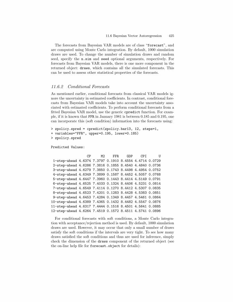
11.6 Bayesian Vector Autoregression 425
The forecasts from Bayesian VAR models are of class “forecast”, andare computed using Monte Carlo integration. By default, 1000 simulationdraws are used. To change the number of simulation draws and randomseed, specify the n.sim and seed optional arguments, respectively. Forforecasts from Bayesian VAR models, there is one more component in thereturned object: draws, which contains all the simulated forecasts. Thiscan be used to assess other statistical properties of the forecasts.
11.6.2 Conditional Forecasts
As mentioned earlier, conditional forecasts from classical VAR models ig-nore the uncertainty in estimated coefficients. In contrast, conditional fore-casts from Bayesian VAR models take into account the uncertainty asso-ciated with estimated coefficients. To perform conditional forecasts from afitted Bayesian VAR model, use the generic cpredict function. For exam-ple, if it is known that FFR in January 1981 is between 0.185 and 0.195, onecan incorporate this (soft condition) information into the forecasts using:
> zpolicy.spred = cpredict(zpolicy.bar13, 12, steps=1,
+ variables="FFR", upper=0.195, lower=0.185)
> zpolicy.spred
Predicted Values:
CP M2 FFR GDP CPI U
1-step-ahead 4.6374 7.3797 0.1910 8.4554 4.4714 0.0729
2-step-ahead 4.6286 7.3816 0.1855 8.4540 4.4840 0.0736
3-step-ahead 4.6279 7.3850 0.1743 8.4498 4.4954 0.0752
4-step-ahead 4.6349 7.3899 0.1587 8.4452 4.5057 0.0768
5-step-ahead 4.6447 7.3960 0.1443 8.4414 4.5149 0.0791
6-step-ahead 4.6525 7.4033 0.1324 8.4406 4.5231 0.0814
7-step-ahead 4.6549 7.4114 0.1270 8.4412 4.5307 0.0835
8-step-ahead 4.6523 7.4201 0.1283 8.4428 4.5383 0.0851
9-step-ahead 4.6453 7.4284 0.1349 8.4457 4.5461 0.0864
10-step-ahead 4.6389 7.4365 0.1432 8.4482 4.5547 0.0876
11-step-ahead 4.6317 7.4444 0.1516 8.4501 4.5641 0.0885
12-step-ahead 4.6264 7.4519 0.1572 8.4511 4.5741 0.0896
For conditional forecasts with soft conditions, a Monte Carlo integra-tion with acceptance/rejection method is used. By default, 1000 simulationdraws are used. However, it may occur that only a small number of drawssatisfy the soft conditions if the intervals are very tight. To see how manydraws satisfied the soft conditions and thus are used for inference, simplycheck the dimension of the draws component of the returned object (seethe on-line help file for forecast.object for details):

426 11. Vector Autoregressive Models for Multivariate Time Series
> dim(zpolicy.spred$draws)
[1] 372 72
In this case, only 372 out of 1000 simulation draws satisfied the con-ditions. To continue simulating from the posterior moment distribution,use the same command as before, with seed set to the current value of.Random.seed:
> zpolicy.spred2 = cpredict(zpolicy.bar13, 12, steps=1,
+ variables="FFR", upper=0.195, lower=0.185, seed=.Random.seed)
> dim(zpolicy.spred2$draws)
[1] 389 72
Note that the draws in zpolicy.spred2 can be combined with the drawsin zpolicy.spred to obtain an updated and more accurate estimate ofconditional forecasts.To ignore the coefficient uncertainty for the conditional forecasts, call
the classical method function cpredict.VAR directly on a fitted BayesianVAR object. The technique introduced above can also be used for classicalprediction with soft conditions.
11.7 References
[1] Campbell, J. A. Lo and C. MacKinlay (1997). The Economet-rics of Financial Markets. Princeton University Press, New Jersey.
[2] Culbertson, K. (1996). Quantitative Financial Economics: Stocks,Bonds and Foreign Exchange. John Wiley and Sons, Chichester.
[3] Doan, T. A., Litterman, R. B., and Sims, C. A. (1984). “Fore-casting and Conditional Projection Using Realistic Prior Distribu-tions”, Econometric Reviews, 3, 1-100.
[4] Granger, C.W.J. (1969). “Investigating Causal Relations by Econo-metric Models and Cross Spectral Methods,” Econometrica, 37, 424-438.
[5] Hamilton, J.D. (1994). Time Series Analysis. Princeton UniversityPress, Princeton.
[6] Lee, B.-S. (1992). “Causal Relations Among Stock Returns, InterestRates, Real Activity, and Inflation,” Journal of Finance, 47, 1591-1603.
[7] Lutkepohl, H. (1991). Introduction to Multiple Time Series Anal-ysis. Springer-Verlag, Berlin.

11.7 References 427
[8] Lutkepohl, H. (1999). “Vector Autoregressions,” unpublished manuscript,Institut fur Statistik und Okonometrie, Humboldt-Universitat zu Berlin.
[9] Mills, T.C. (1999). The Econometric Modeling of Financial TimeSeries, Second Edition. Cambridge University Press, Cambridge.
[10] Runkle, D. E. (1987). “Vector Autoregressions and Reality,” Jour-nal of Business and Economic Statistics, 5 (4), 437-442.
[11] Sims, C.A. (1980). “Macroeconomics and Reality,” Econometrica,48, 1-48.
[12] Sims, C. A., and Zha, T. (1998). “Bayesian Methods for DynamicMultivariate Models”, International Economic Review, 39 (4), 949-968
[13] Stock, J.H. and M.W. Watson (2001). “Vector Autoregressions,”Journal of Economic Perspectives, 15, 101-115.
[14] Tsay, R. (2001). Analysis of Financial Time Series. John Wiley &Sons. New York.
[15] Watson, M. (1994). “Vector Autoregressions and Cointegration,” inHandbook of Econometrics, Volume IV. R.F. Engle and D. McFadden(eds.). Elsevier Science Ltd., Amsterdam.
[16] Waggoner, D. F., and Zha, T. (1999). “Conditional Forecasts inDynamic Multivariate Models,” Review of Economics and Statistics,81 (4), 639-651.
[17] Zha, T. (1998). “Dynamic Multivariate Model for Use in FormulatingPolicy”, Economic Review, Federal Reserve Bank of Atlanta, FirstQuarter, 1998.


![Lattice filter based multivariate autoregressive spectral ...the Wigner-Ville spectral analysis [3] and the Priestley’s evolutionary spectra framework [4], [5]. The time-varying](https://static.fdocuments.in/doc/165x107/61270aa68b9fe23ec7093b3a/lattice-ilter-based-multivariate-autoregressive-spectral-the-wigner-ville.jpg)