UNIVERSITA DEGLI STUDI ROMA TRE` - CERNcds.cern.ch/record/1160294/files/CERN-THESIS-2009-005.pdf ·...
108
CERN-THESIS-2009-005 22/01/2009 UNIVERSIT ` A DEGLI STUDI ROMA TRE Facolt` a di Scienze Matematiche Fisiche e Naturali Dottorato di ricerca in Fisica — XXI ciclo Tesi di Dottorato A design study of the production of Z bosons in association with b jet in final states with muons with the ATLAS detector at the LHC Sara Diglio Supervisore: Coordinatore: Prof. Filippo Ceradini Prof. Guido Altarelli
Transcript of UNIVERSITA DEGLI STUDI ROMA TRE` - CERNcds.cern.ch/record/1160294/files/CERN-THESIS-2009-005.pdf ·...

CER
N-T
HES
IS-2
009-
005
22/0
1/20
09
UNIVERSIT A DEGLI STUDI ROMA TRE
Facolta di Scienze Matematiche Fisiche e Naturali
Dottorato di ricerca in Fisica — XXI ciclo
Tesi di Dottorato
A design study of the production ofZ bosons in associationwith b jet in final states with muons
with the ATLAS detector at the LHC
Sara Diglio
Supervisore: Coordinatore:Prof. Filippo Ceradini Prof. Guido Altarelli

A nonna Maria

“Les hommes chez toi”, dit le petit prince, “cultivent cinq mille roses dans un memejardin ... et ils n’y trouvent pas ce qu’ils cherchent ...”
“Ils ne trouvent pas”, repondis-je.“Et cependant ce qu’ils cherchent pourraitetre trouve dans en seule rose ou un peu
d’eau ...”“Bien sur”, r epondis-je.Et le petit prince ajouta:“Mais les yeux sont aveugles. Il faut chercher avec le coeur”.
“The men where you live”, said the little prince, “grow five thousand roses in thesame garden ... and they do not find what they are looking for ...”
“They do not find it”, I replied.“And yet, what they are looking for could be found in a single rose or in a little
water ...”“Yes, indeed,”, I replied.And the little prince added:“But the eyes are blind. One must look with the heart”.
“Da te, gli uomini”, disse il piccolo principe, “coltivano cinquemila rose nellostesso giardino ... e non trovano quello che cercano ...”
“Non lo trovano”,risposi.“E tuttavia quello che cercano potrebbe essere trovato in una sola rosa o in un po’
d’acqua ...”“Certo”, risposi.E il piccolo principe soggiuse:“Ma gli occhi sono ciechi. Bisogna cercare col cuore”.
Antoine de Saint Exupery

Contents
Introduction 1
1 Theoretical Overview 31.1 Standard Model of Particle Physics . . . . . . . . . . . . . . . . . .. . . . . . 3
1.1.1 Matter particles and force carriers . . . . . . . . . . . . . . .. . . . . 31.1.2 Gauge Symmetries . . . . . . . . . . . . . . . . . . . . . . . . . . . . 5
1.2 Electroweak Theory . . . . . . . . . . . . . . . . . . . . . . . . . . . . . . .. 61.2.1 Electro Weak Symmetry Breaking . . . . . . . . . . . . . . . . . . . .81.2.2 Phenomenology of Higgs Boson . . . . . . . . . . . . . . . . . . . . . 8
1.3 Theory of Strong Interaction . . . . . . . . . . . . . . . . . . . . . . .. . . . 121.3.1 Parton Model . . . . . . . . . . . . . . . . . . . . . . . . . . . . . . . 121.3.2 Hadron-Hadron collision . . . . . . . . . . . . . . . . . . . . . . . .. 13
1.4 Beyond the Standard Model . . . . . . . . . . . . . . . . . . . . . . . . . . .141.4.1 Limitations of the Standard Model . . . . . . . . . . . . . . . . .. . . 141.4.2 Super Symmetry . . . . . . . . . . . . . . . . . . . . . . . . . . . . . 15
2 Experimental Apparatus 182.1 The LHC Accelerator Complex . . . . . . . . . . . . . . . . . . . . . . . . .. 182.2 The ATLAS Detector . . . . . . . . . . . . . . . . . . . . . . . . . . . . . . . 20
2.2.1 The coordinate system and nomenclature . . . . . . . . . . . .. . . . 202.2.2 Physics requirements . . . . . . . . . . . . . . . . . . . . . . . . . . .22
2.3 Magnetic System . . . . . . . . . . . . . . . . . . . . . . . . . . . . . . . . . 242.4 Inner Detector . . . . . . . . . . . . . . . . . . . . . . . . . . . . . . . . . . .252.5 Calorimeter System . . . . . . . . . . . . . . . . . . . . . . . . . . . . . . . .272.6 Muon System . . . . . . . . . . . . . . . . . . . . . . . . . . . . . . . . . . . 29
2.6.1 Muon Chamber Types . . . . . . . . . . . . . . . . . . . . . . . . . . 312.7 The Trigger and Data Acquisition System . . . . . . . . . . . . . .. . . . . . 34
3 Software tools 373.1 Monte Carlo Events Generators . . . . . . . . . . . . . . . . . . . . . . .. . . 39
3.1.1 The QCD model . . . . . . . . . . . . . . . . . . . . . . . . . . . . . 403.1.2 Parton Density Function (PDF) . . . . . . . . . . . . . . . . . . . .. 433.1.3 Generator parameters . . . . . . . . . . . . . . . . . . . . . . . . . . .45
3.2 The Full detector simulation and reconstruction . . . . . .. . . . . . . . . . . 453.2.1 GEANT4 Simulation . . . . . . . . . . . . . . . . . . . . . . . . . . . 463.2.2 Offline reconstruction . . . . . . . . . . . . . . . . . . . . . . . . . .46
I

CONTENTS II
3.3 The Fast detector simulation and reconstruction . . . . . .. . . . . . . . . . . 513.3.1 Reconstruction algorithms . . . . . . . . . . . . . . . . . . . . . . .. 51
4 Studies using the FULL simulation 544.1 Introduction . . . . . . . . . . . . . . . . . . . . . . . . . . . . . . . . . . . .544.2 Monte Carlo Data Samples and Cross Sections . . . . . . . . . . . . .. . . . 554.3 Events Selection . . . . . . . . . . . . . . . . . . . . . . . . . . . . . . . . .. 57
4.3.1 Trigger Selection . . . . . . . . . . . . . . . . . . . . . . . . . . . . . 574.3.2 Muons . . . . . . . . . . . . . . . . . . . . . . . . . . . . . . . . . . 584.3.3 Jets . . . . . . . . . . . . . . . . . . . . . . . . . . . . . . . . . . . . 594.3.4 Jet tagging . . . . . . . . . . . . . . . . . . . . . . . . . . . . . . . . 604.3.5 Tests of b-tagging . . . . . . . . . . . . . . . . . . . . . . . . . . . . . 614.3.6 Event selection efficiency . . . . . . . . . . . . . . . . . . . . . . .. 63
4.4 Number of events and ratio of cross sections . . . . . . . . . . .. . . . . . . . 654.4.1 Number of events . . . . . . . . . . . . . . . . . . . . . . . . . . . . . 654.4.2 Ratio of cross sections . . . . . . . . . . . . . . . . . . . . . . . . . . 68
4.5 b-tagging algorithm using pp→ W (µν) inclusive sample . . . . . . . . . . . 694.5.1 Events Selection and Results . . . . . . . . . . . . . . . . . . . . . .. 69
5 Studies using the FAST simulation 715.1 Preliminary studies ofb density function . . . . . . . . . . . . . . . . . . . . . 71
5.1.1 Monte Carlo Data Samples . . . . . . . . . . . . . . . . . . . . . . . . 715.1.2 b parton and b jets distributions . . . . . . . . . . . . . . . . . .. . . 72
5.2 Studies of background from Z+c-jet . . . . . . . . . . . . . . . . . .. . . . . 745.2.1 Simulated Data Sample and Event selection . . . . . . . . . .. . . . . 755.2.2 Impact parameter and invariant mass tracksb-tagging . . . . . . . . . . 785.2.3 Soft muon b-tagging . . . . . . . . . . . . . . . . . . . . . . . . . . . 83
6 Systematics Uncertainties 936.1 Jet Energy scale . . . . . . . . . . . . . . . . . . . . . . . . . . . . . . . . . .936.2 PDF . . . . . . . . . . . . . . . . . . . . . . . . . . . . . . . . . . . . . . . . 946.3 b-tagging algorithm . . . . . . . . . . . . . . . . . . . . . . . . . . . . . .. . 95
Conclusions 96
Acknowledgements 98
Bibliography 99

Introduction
The Large Hadron Collider (LHC) is the machine that will provide the highest ever producedenergy in the center of mass, reaching the value of
√s=14 TeV for proton-proton collisions and
giving the possibility to produce particles with mass up to few TeV. The main aim of the LHCexperiments is the search for the Higgs boson, which is fundamental to verify the symmetry-breaking mechanism in the electroweak sector of the Standard Model Theory. In addition theLHC experiments will explore the existence and the predictions of possible supersymmetricmodels and will perform precision measurements of the heavyquarks.Four experiments are actually under commissioning phase onthe LHC: ATLAS and CMS aretwo general purpose experiments, LHCb is mainly dedicated toCP symmetry violation studiesand ALICE is going to exploit the heavy ions physics.The work presented in this thesis is carried on in the framework of the ATLAS experiment. Itpresents a study of the prospects for measuring the production of a Z boson in association to bjet. This process is interesting in its own and also as background for many Standard Model andbeyond Standard Model physics processes.The wide kinematic range for production of Z + b jet serves as atesting ground for perturbativeQCD predictions. In addition the cross section is sensitive to the b quark content in the protonand its precise measurement will help in reducing the current uncertainty on the partonic con-tent of the proton (PDF’s). Such uncertainty is presently affecting the potential for discoveringnew physics at LHC.
The motivations to study this process at LHC appear even moreevident from the compari-son with the Tevatron cross sections [19]. First of all, the total cross section for Z+b productionat LHC is about a factor of 50 larger than at the Tevatron. Moreover the cross section for Z+cproduction compared to Z+b is more important at Tevatron than at LHC. In general at the LHC,the relative importance of processes other than Z+b (such asZc, Zq and Zg) is less relevant thanat the Tevatron. Finally, the probability of mis-tagging a light jet as a heavy quark is smaller,therefore the LHC provides a cleaner environment for the extraction of the Z+b signal.Z+b jet events will be also used to calibrate the calorimetric b jet energy measurements, profit-ing from the high statistics and a relative low and well knownbackground. It will be possibleto calibrate the calorimeters using jets reconstructed in the experiment, performing an “in situcalibration” [40–42].
The study of the pp→ Z + b jet channel has been done considering the decay selection Z→ µ+µ− and the identification of the b jet both in an inclusive mode and through the semi-leptonic decay of the b jet into muons. The choice of final states with muons is due to a betteridentification of the final state (through the isolated muons).
1

CONTENTS 2
This thesis describes analysis strategies developed to extract the signal from his possible back-grounds and presents the results obtained. In this work computing tools were developed andtested extensively. The study was performed using the signal and background events modelledwith Monte Carlo generators, many of which have been newly developed for the LHC analyses.Full and fast simulation of the Atlas detector was performedto obtain realistic estimates of thesensitivity of the measurements.
Chapter 1 is dedicated to a theoretical overview on the state of art in particle physics in orderto introduce the topics that will be recovered in subsequentchapters.A general overview of the ATLAS experiment is given in chapter 2.Chapter 3 summarizes the software tools inside the Athena framework that have been used toperform the analysis.Chapter 4 is dedicated to the studies performed using fully simulated data, while in chapter 5 thesystematic studies on b PDF and mistagging of c jets using fast simulated samples are shown.A summary of the main sources of systematic uncertainties onZ+ b jet cross section measumentis discussed in chapter 6.
Chapter 1
Theoretical Overview
This chapter presents a basic overview of the Standard Modelthat describes the current under-standing of fundamental matter particles and their interactions.
In the following I will briefly discuss the basic themes and limits of the Standard Modelfocusing the attention on the ones related to this thesis.
1.1 Standard Model of Particle Physics
The Standard Model (SM) of particle physics is the Quantum Field Theory (QFT) that todayprovides the best description of fundamental particles andtheir interactions. It identifies struc-tureless, elementary particles that constitute all the observed matter in the universe: these arethequarksandleptons. The interactions between the quarks and leptons are mediated by parti-cles calledgauge bosons. The Standard Model provides the theoretical framework to calculatephysical (measurable) quantities, explains observed phenomena, and make predictions that canbe checked experimentally. It has been enormously successful in explaining and predicting theresults: most of these predictions have been confirmed to spectacular precision (many at CERN,Fermilab, SLAC).
Despite its many successes, there is consensus among particle physicists that the StandardModel is not the final theory of particle physics.
1.1.1 Matter particles and force carriers
The Standard Model describes the constituents of matter andtheir interactions in terms of funda-mental point-like particles. A peculiar property of particles is their internal angular momentumcalledspin. The particles can be considered in two categories: the fundamental fermionic par-ticles whose spin is12h and gauge bosons whose spin is 1h.The matter is made off ermionscalledquarksandleptonsand their interactions are describedby the exchange ofgauge bosons.
The properties of the Standard Model particles are summarized in Table 1.1.The quarks and leptons can be arranged in generations (see Table 1.2).Among the three quark generations a mixing mechanism existsthat is parametrized by the
3

CHAPTER 1. THEORETICAL OVERVIEW 4
Flavor Electric Spin Mass (GeV) Baryon Le Lµ LτCharge (e) Number
Quarksu (up) +2/3 1/2 0.0015–0.004 1/3 0 0 0d (down) −1/3 1/2 0.004–0.008 1/3 0 0 0c (charm) +2/3 1/2 1.15–1.35 1/3 0 0 0s (strange) −1/3 1/2 0.08–0.13 1/3 0 0 0t (top) +2/3 1/2 178 1/3 0 0 0b (bottom) −1/3 1/2 4.1–4.4 1/3 0 0 0
Leptonse (electron) -1 1/2 0.511× 10⁻³ 0 1 0 0νe (electron neutrino) 0 1/2 <3× 10⁻⁹ 0 1 0 0µ (muon) -1 1/2 0.106 0 0 1 0νµ (muon neutrino) 0 1/2 <1.9× 10⁻⁴ 0 0 1 0τ (tau) -1 1/2 1.78 0 0 0 1ντ (tau neutrino) 0 1/2 <1.8× 10⁻² 0 0 0 1
Gauge BosonsW± (charged weak) ±1 1 80.403± 0.029 0 0 0 0Z0 (neutral weak) 0 1 91.1876± 0.0021 0 0 0 0γ (photon) 0 1 0 0 0 0 0gi (i=1,...,8 gluons) 0 1 0 0 0 0 0g (graviton) 0 2 0 0 0 0 0
Table 1.1: The fundamental particles of the Standard Model and some of their properties. Le,Lµ , and Lτ are the electron, muon, and tau lepton numbers [1]. For everyparticle there is acorresponding antiparticle.
Cabibbo-Kobayashi-Maskawa matrix (that will be discussed in section 1.2). The StandardModel does not explain the origin of such a mixing.Analysis on the Z partial decay width into hadrons, leptons and neutrinos at LEP indicates thatthere are exactly three families of light neutrinos (assuming lepton universality). Strict lowerlimits have been set on the mass of 4th generation quarks and leptons.
Generation 1 Generation 2 Generation 3u c td s bνe νµ ντe µ τ
Table 1.2: The fundamental particles of the Standard Model grouped into generations. Themain difference between the generations is the masses of their particles.
Quarks do not exist as free particles: different combinations of quarks form the spectrum ofparticles called hadrons. This item will be discussed in more detail in section 1.3.1.
CHAPTER 1. THEORETICAL OVERVIEW 5
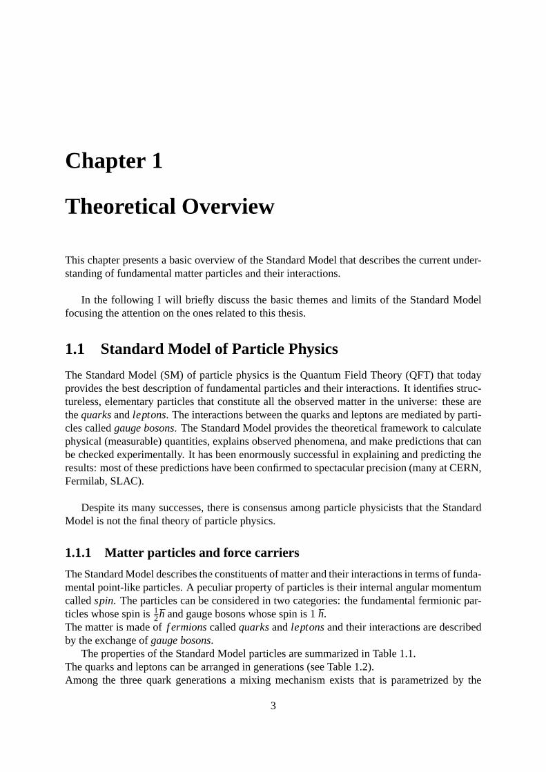
The weak bosons (W± and Z0) and photon (γ) mediate the electroweak force. Gluons arethe mediators of the strong force. An example of force exchange between quarks and gluonsinteracting through vector bosons is shown in figure 1.1.
Figure 1.1: Feynman diagrams showing the basic forms of the electromagnetic, weak and stronginteractions between two fermions mediated by the exchangeof a photon,W±/Z0 and a gluon.
1.1.2 Gauge Symmetries
The fundamental particle interactions described by the Standard Model are the following:
• electromagnetic;
• weak;
• strong.
These interactions can be described as a combination of three unitary gauge groups, denotedas SU(3)⊗ SU(2)⊗ U(1) [2]. The group SU(3) is the symmetry group of strong interactions,U(1) describes electromagnetic interactions, and SU(2)⊗ U(1) represents the unified weak andelectromagnetic interaction.
These symmetries are of prime importance in particle physics. To illustrate this point, con-sider that observables depend on the wave function squared (|Ψ|2). If local gauge invarianceholds, the transformation
Ψ→ Ψ′= e−iχ(~x,t)Ψ (1.1)
whereχ(~x, t) is an arbitrary phase which can depend on space and time coordinates, shouldleave the observables unchanged. Physically, since the absolute phase cannot be measured, the

CHAPTER 1. THEORETICAL OVERVIEW 6
choice of phase should not matter. If one successively inserts Ψ andΨ′into the Schrodinger
equation for a matter particle,
12m
▽2 Ψ(~x, t) = i∂Ψ(~x, t)
∂ t, (1.2)
the equation is clearly not invariant under the transformation of equation 1.1.To guarantee gauge invariance the Schrodinger equation should be modified. For electrically
charged particles, the modified Schrodinger equation is
12m
(−i~∇ +e~A
)2Ψ =
(i∂∂ t
+eV
)Ψ, (1.3)
wheree is the electric charge,V is the electric potential, and~A is the vector potential. With thischange, the Schrodinger equation is invariant under the simultaneous transformations (1.1) and
A→ A′= A+
1e▽ χ (1.4)
V →V′= V − 1
e∂ χ∂ t
. (1.5)
Thus, the requirement that the theory be locally gauge invariant leads to the required presenceof a field Aµ =(V;~A). Further, since particles are viewed as excitations of fields in this theory,the requirement of gauge invariance also leads to the presence of gauge bosons.
In the Standard Model, phase symmetries (mathematically, requirements that the theory beinvariant under gauge transformations) are used to guide the construction of theories. The gaugefields and particles follow naturally from these symmetries.The gauge theories introduced above involve only massless gauge bosons. However, massivegauge bosons (W±,Z0) have been observed experimentally. Evidence of a mechanism thatcauses the gauge bosons to acquire their masses is highly sought in particle physics. Currently,the leading candidate is the Higgs mechanism that will be discussed in section 1.2.1.
1.2 Electroweak Theory
The electroweak model is a gauge theory based on thebrokensymmetry groupSU(2)L⊗U(1)Y.The weak hypercharge (Y) is related to the third component of the weak isospin (I3) and to theelectric charge through the formula:
Q = I3 +Y2
(1.6)
The fermions are introduced inleft-handed (L)doublets andright-handed(R) singlets.Handedness is related to the helicity of the fermion: the component of spin along its direction ofmotion. Quantum numbers ofleft-handed(L) and right-handed(R) fermions are summarizedin table 1.3. The anti-fermions eigenvalues have opposite sign.
The relation between the coupling costants of weak and electro magnetic interactions is

CHAPTER 1. THEORETICAL OVERVIEW 7
νeL,νµL,ντ L eL,µL,τL eR,µR,τR uL,cL, tL d′L,s
′L,b
′L uR,cR, tR d′
R,s′R,b′RI 1
212 0 1
212 0 0
I3 +12 −1
2 0 +12 −1
2 0 0Y -1 -1 -2 +1
3 +13 +4
3 −23
Q 0 -1 -1 +23 −1
3 +23 −1
3
Table 1.3: SU(2)⊗ U(1) quantum numbers of left-handed and right-handed fermions.
e= g·sinθW (1.7)
wheree is the electric charge of the electron,g is the weak coupling costant,θW is theWeinberg’s angle, that can be measured in theν −ediffusion, or in the electroweak interferencein e+e− processes betweenγ and Z exchange, or studying theZ width or also from the ratiobetween masses of theW± and of theZ.The combined analysis of those experiments quoted the following result [1]:
sin2θW = 0.23113±0.0005 (1.8)
TheW boson couples to quarks and lepton always with the same chiral status (maximumparity violation). TheZ boson coupling depends also from the electric charge of fermions. Theforce of this coupling with a generic fermionf can be expressed as:
gZ( f ) =g
cosθW· (I3−zf ·sin2θW) (1.9)
wherezf is the electric charge of the fermion in elementary electricchargee units andI3 isthe third component of the weak isospin.
Coupling constants for left-handed or right-handed fermions are different (see table 1.4).They can be written as
gL = I3−zf ·sin2θW (1.10)
gR = −zf ·sin2θW (1.11)
νe,νµ ,ντ e,µ,τ u,c, t d′,s′,b′
gL12 −1
2 +sin2θW12 − 2
3 ·sin2θW −12 + 1
3 ·sin2θW
gR 0 +sin2θW −23 ·sin2θW
13 ·sin2θW
Table 1.4: Couplings between theZ boson and fermions
In addition, the mass eigenstates are not eigenstates of theweak interaction of quarks: theyare mixed, parameterised by three mixing angles and one phase angle according to the Cabibbo-Kobayashi-Maskawa (CKM) formalism.

CHAPTER 1. THEORETICAL OVERVIEW 8
d′
s′
b′
=
Vud Vus Vub
Vcd Vcs Vcb
Vtd Vts Vtb
·
dsb
(1.12)
The values of the magnitudes of the elements of the matrix as quoted in [1], assuming thematrix is unitary, are
VCKM =
0.9739−0.9751 0.221−0.227 0.0029−0.00450.221−0.227 0.9730−0.9744 0.039−0.0440.0048−0.014 0.037−0.043 0.9990−0.9992
(1.13)
Each generation has a small off-diagonal mixing element leading to coupling betweenquarks of different generations. Flavor mixing in the lepton sector was in fact confirmed in1998, implying that neutrinos have non-zero mass. However,this effect is even smaller thanquark mixing and the coupling of leptons with different doublets is minute.
1.2.1 Electro Weak Symmetry Breaking
The electroweak model is passing experimental tests with high precision. However, the symme-try in the electroweak model requires all four bosons to be massless. This is obviously a brokenassumption as we observe very massive weak bosons.In 1964 Franois Englert, Robert Brout, Peter Higgs and independently Gerald Guralnik, C. R.Hagen, and Tom Kibble conjectured that the massless gauge bosons of weak interactions ac-quire their mass through interaction with a scalar field (theHiggs Field), resulting in a singlemassless gauge boson (the photon) and three massive gauge bosons (W± and Z0) [3–5]. Thisis possible because the Higgs field has a potential function which allows degenerate vacuumsolutions with a non-zero vacuum expectation value.The interaction between the particle and this Higgs field contributes to the particles energy re-spect to the vacuum. This energy is equivalent to a mass. In the minimal Standard Model onlya doublet of scalar fields is introduced. In the simplest model masses of quarks, leptons andbosons are all interpreted as the interaction with a unique scalar field. Particles which interactstrongly are the heaviest, while particles that interacts weakly are lighter. There is always aparticle associated to a quantum field, so the theory predicts the observation of a spin-0 Higgsboson which is now the only remaining particle to be discovered within the Standard Model.Several theories have been proposed which include the Higgsmechanism to give the gaugebosons masses. In those theories more than one Higgs boson ispredicted. Among all the theo-ries there is SuperSymmetry (SUSY) that will be briefly discussed in section 1.4.2.
1.2.2 Phenomenology of Higgs Boson
As it was discussed in the previous section, the Standard Model predicts the existence of ascalar neutral boson that is the results of the spontaneous electroweak symmetry breakingSUL(2)⊗UY(1).

CHAPTER 1. THEORETICAL OVERVIEW 9
The Higgs boson couples to quarks and leptons with a force proportional to(g·mf )/(2mW)whereg is the coupling costant of the gauge theorySUL(2) andmf is the fermion mass.The Higgs mass is related to the Higgs potential parametersν andλ as: mH =
√2v2λ . The
parameterν is the vacuum expectation value of the Higgs field that is predicted by the theoryν=246 GeV. In spite of this prediction the theory is not able topredict the value for the realparameterλ and as a consequence neither the value for the Higgs mass. It is possible only tofix some theoretical constraints to the Higgs particle mass as a function of the energy scale atwhich the Standard Model is valid. Those limits are shown in figure 1.2.
Figure 1.2: Theoretical limits on the Higgs boson mass as a function of the energy scaleΛuntil which the Standard Model is valid. The thickness of thebands indicates the theoreticaluncertainties.
Figure 1.2 shows a very important feature: if the Higgs bosonexists and his mass is be-tween∼ 150 GeV
c2 and∼ 180 GeVc2 the Standard Model could be valid until Planck mass scale
∼ 1019GeVc2 .
From an experimental point of view, lower limits onmH come from direct measurements doneat Tevatron [20] and LEP (Large Electron Positron collider)[12]. A global fit on LEP and Teva-tron data withmH treated as free parameter is in figure 1.3. The global fit to theelectroweakdata givesmH = 84+34
−26 Direct searches at LEP gave a lower limit ofmH > 114.3GeV at 95%confidence level.
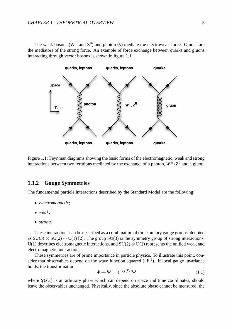
Thanks to the high luminosity and to an energy never reached by any other collider (14 TeVin the center of mass), at LHC it will be possible to investigate the origin of the spontaneoussymmetry-breaking mechanism in the electroweak sector of the Standard Model looking for theHiggs boson.The theoretical production cross sections for the Higgs boson at LHC as a function of the bosonmass is shown in figure 1.4. Feynman diagrams of the principalproduction mechanisms atthe LHC are shown in figure 1.5, while the Higgs Branching Ratios(BR) decay channels as afunction of the Higgs mass are shown in figure 1.6.
As it can be seen in figure 1.6 , formH < 130 GeVH → bb is the most favourite channel,

CHAPTER 1. THEORETICAL OVERVIEW 10
bb being the heaviest fermion pair accessible to the Higgs.I want to focus the attention on the process (d) in figure 1.5 when an Higgs is produced inassosiation to aZ boson: this process can be mimed by the process object of thisthesis (Z +b jets) wheneverb andb from the Higgs decay are not resolved as two different jets (see fig1.7) [17,18].
0
1
2
3
4
5
6
10030 300
mH [GeV]
∆χ2
Excluded Preliminary
∆αhad =∆α(5)
0.02758±0.00035
0.02749±0.00012
incl. low Q2 data
Theory uncertaintyJuly 2008 mLimit = 154 GeV
Figure 1.3: Global fit to the electroweak data as a function ofmH . The band represents anestimate of the theoretical error due to missing higher order corrections. The vertical bandshows the 95% CL exclusion limit onmH from the direct search. [12].
Figure 1.4: Production cross sections for the Higgs boson atLHC as a function of the bosonmass.
CHAPTER 1. THEORETICAL OVERVIEW 11
Figure 1.5: Diagrams of the main production processes of theHiggs boson: (a) gluon gluonfusion, (b)Z or W fusion, (c) associated production withtt pair, (d) associated production withaZ or W boson.
Figure 1.6: Branching Ratios of Higgs decays as a function of the Higgs mass.
Figure 1.7: Diagrams: (a) associated production of anHiggsdecaying intob with a Z boson;(b) associated production of aZ boson with a b-jet.

CHAPTER 1. THEORETICAL OVERVIEW 12
1.3 Theory of Strong Interaction
This section introduces the theory of the strong interactions also calledQuantum Chromo Dy-namics(QCD). The main features of QCD that are relevant to understandand describe thehadron structure and calculate the evolution of partons that constitute hadrons will be discussedin the following.
1.3.1 Parton Model
According to theParton Modelthe hadrons are strongly interacting particles built fromvalencequarksthat define the quantum numbers (charge, spin, isospin) of the hadrons and fromseaquarksthat result from the gluon splitting inside the hadrons. Thefundamental particles thatconstitue the hadrons (quarksandgluons) are calledpartons.It is possible to distinguish between two different combinations of valence quarks that giveorigin to two different families of hadrons:
• MESONSqq;
• BARYONS qqq(ANTI-BARYONS qqq).
As an example the proton is a baryon made from the combination{uud}. The charge ofthe proton (in units of the electron charge) is the sum of the charges of its constituent quarks,2/3+2/3+(−1/3) = +1, its baryon number is 1, and its lepton number is 0 (baryon numberand lepton number are additive quantum numbers. See Table 1.1). A neutron is made from thecombination{udd}. It has electric charge 2/3+(−1/3)+(−1/3) = 0, baryon number 1, andlepton number 0. The success of the quark model in explainingand predicting other experimen-tally observed states led to its acceptance.Despite this success, there are problem with this simplicistic description: the combination{uuu} has been observed as the∆++ baryon. The existence of the∆++ presents a problembecause its spin, J= 3/2, is obtained by combining three identical fermions with the samequantum numbers. This violates Fermi statistics. Another problem is that neither combinationsof more than three quarks or single quarks are observed.The solution to these problems is the introduction of another quantum number called color. Itcan have one of three values, called red (R), green (G), and blue (B), with antiquarks havingthe valuesR, G, andB. In QCD, bound states must be colorless, so mesons are formed fromone quark and one antiquark which carry a color and its anti-color (like RR), while baryons areformed from three quarks, one of each color, in an antisymmetric combination. Thus the∆++
baryon consists of one u quark of each color.Color is exchanged between quarks and gluons (both of which carry a color charge). Gluonsare the mediators of the strong force. They are colored objects that carry color charge.Unlike photons, which mediate a force that gets weaker with distance, gluons are responsiblefor a binding force that strengthens with distance.Gluons (and quarks) are colored, so cannot be observed directly because bound states areformed only as colorless objects. This behaviour is called color confinement. Eventually, whencolored objects are pulled apart from other colored objects(as occurs in high-energy collisions),

CHAPTER 1. THEORETICAL OVERVIEW 13
the energy released is converted into new colored objects, and colorless objects are formed fromgroups of the colored objects. Only colorless objects are observed in particle detectors and aredetected as streams, or jets, of particles. It should be emphasized that leptons do not carry acolor charge, and thus do not feel the strong force. This is the distinction between quarks andleptons.
1.3.2 Hadron-Hadron collision
According to QCD the observed hadrons are composite particles made of partons (quarks andgluons). The quarks and gluons are the fundamental degrees of freedom to participate in strongreactions at high energies. The collision between two hadrons (two protons at the LHC) canbe described as an interaction between partons that constitute the hadrons. A scheme of thisinteraction is shown in figure 1.8.
Figure 1.8: Simplified scheme of hadron-hadron interaction.
Scattering processes at high-energy hadron colliders can be classified as either hard or soft.Quantum Chromodynamics (QCD) is the underlying theory for allsuch processes, but the ap-proach and level of understanding is very different for the two cases. For hard processes, e.g.Higgs boson or highpT jet production, the rates and event properties can be predicted with goodprecision using perturbation theory. For soft processes the rates and properties are dominatedby non-perturbative QCD effects, which are less understood.Assuming that the masses of the partons are negligible and that the transferred quadri-momentumQ from the initial to the final state satisfied the relationQ2 ≫ M2 (whereM is the mass of thehadron), theBjorken scale variableis defined:
x =Q2
2Mν(1.14)
Being ν the energy transfer in the interaction, thex variable represents the fraction of thequadri-momentum of the hadron carried by the interacting parton.The available energy in the center of mass of the collision,
√s, is related to the total energy in
the center of mass√
s through the two Bjorken variables (one for each interacting parton) bythe relation:

CHAPTER 1. THEORETICAL OVERVIEW 14
s= x1x2s (1.15)
wherex1 is the fraction of the quadri-momentum carried by the first parton belong to aninteracting hadron andx2 is the one carried by the second parton belong to the other interactinghadron (see fig. 1.8).
In the following I will discuss how the so calledQCD factorization theoremcan be usedto calculate a wide variety of hard-scattering cross sections in hadron- hadron collisions. TheQCD factorization theorem states that the cross sections of high energy hadronic reactions witha large momentum transfer can be factorized into a parton-level hard scattering convoluted withthe parton distribution functions.Theoretical predictions for processes at high transferredquadri-momentumQ are based on thefollowing formula, which relies on the factorization theorem:
σH1H2 = ∑a,b
∫dx1dx2 fa,H1(x1,Q
2) fb,H2(x2,Q2)× σa,b(x1,x2,Q
2) (1.16)
where fc,H(x,Q2) is the parton density function (PDF) of the partonc carrying a fractionx ofthe hadronH momentum andσa,b is the parton-parton hard scattering cross-section describingthe partonic reaction at the scaleQ2.
The parton-level hard scattering cross section can be calculated perturbatively in QCD,while the parton density functions parameterize the non-perturbative aspect and can be onlyobtained by some ansatz and by fitting the data.A more detailed description of parton density function willbe given in section 3.1.2.
1.4 Beyond the Standard Model
As said before there are indications that the Standard Modelis not the final theory of particlephysics and that more fundamental physics is left to be discovered. Experiments in the yearsahead will give insight into which, if any, of the proposed theoretical extensions to the StandardModel is correct. In this section, a few of the reasons for theextensions are discussed.
1.4.1 Limitations of the Standard Model
One reason for introducing an extension to the Standard Model is revealed when calculationsusing the Standard Model framework include a Higgs boson. The inclusion of the Higgs bosonin the theory leads to unphysical results in some calculations. Perturbative calculations of themass of the Higgs boson squared have quadratic divergences.Infinite terms appear in the sum.It is theoretically possible to introduce counterterms in the perturbation series which cancelthese divergences, but this has no physical justification, and is considered unnatural.
A second reason arises from the fact that several theoretical unifications of forces havealready occurred. Electricity and magnetism were once thought of as unrelated, as were theelectromagnetic and weak forces. Thus, many theorists expect that a theory that unifies all ofthe forces should be the final theory. The Standard Model separates the unified electroweak
CHAPTER 1. THEORETICAL OVERVIEW 15
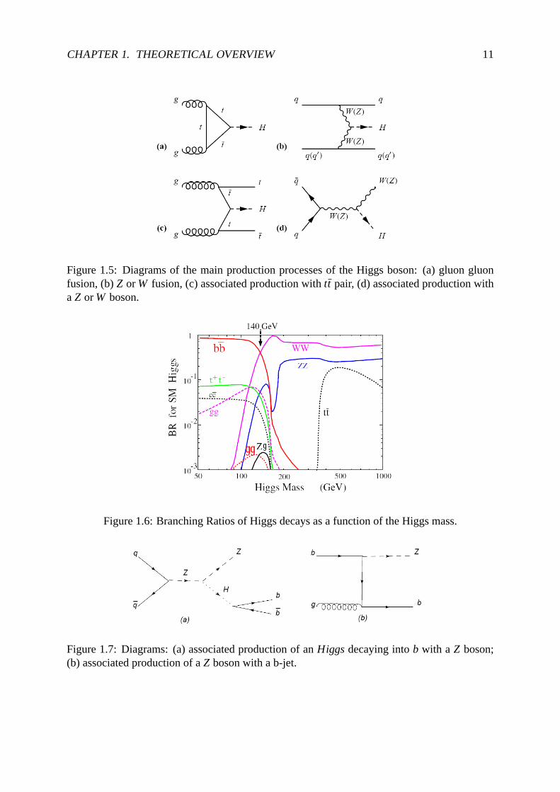
Figure 1.9: Evolution of the coupling strengths as a function of energy in the Standard Model,whereα1 corresponds to U(1) (electromagnetic force),α2 corresponds to SU(2) (electroweakforce), andα3 corresponds to SU(3) (strong force). Diagram from [8].
forces from the strong force, and does not include gravity.The fundamental forces are each characterized by a couplingstrength. The coupling strengthappears in all physical calculations, and is indicative of the strength of the interaction. Thesecoupling strengths have a dependence on the interaction energy; more precisely, they depend onthe momentum transferQ between two particles involved in an interaction. Figure 1.9 showsthe values of the coupling strengths as a function ofQ. Theoretical calculations in the StandardModel predict that the coupling strengths are closer at highenergies than at lower energies. Theexperimental data taken so far agree. However, the couplingstrengths will not meet exactlywithout the existence of some new physics which affects their dependence on the energy. Su-persymmetry is one candidate for this new physics.
1.4.2 Super Symmetry
Supersymmetry is a proposed symmetry which relates fermions to bosons [6]. It postulatesthat for every particle there is a corresponding sparticle,identical to the particle but with a spindifferent by 1/2. If it exists, supersymmetry must be a broken symmetry because no sparticleshave been detected with masses equal to the Standard Model particles.
Supersymmetry solves the problems raised in section 1.4.1,including Higgs bosons to givemass to the particles. It introduces new terms into the calculation of the Higgs mass squaredwhich cancel the terms that lead to the quadratic divergence. It also modifies the evolution ofthe coupling constants so that they unify at a high energy (see figure 1.10).
An example of spectrum of supersymmetric sparticles corresponding to the particles of theStandard Model is shown in table 1.5.
Note that in supersymmetry there are multiple Higgs bosons,and that the observable gaugesparticles are formed as mixtures of the superpartners of the Standard Model gauge particles.The superpartners are technically flavor eigenstates. There is one flavor eigenstate correspond-ing to each degree of freedom of the Standard Model particles. The observable spectrum of

CHAPTER 1. THEORETICAL OVERVIEW 16
Figure 1.10: The evolution of the coupling strengths as a function of energy in supersymmetry,whereα1 corresponds to U(1) (electromagnetic force),α2 corresponds to SU(2) (electroweakforce), andα3 corresponds to SU(3) (strong force).
Standard particles Supersymmetric partnersElectric Particle Spin Sparticle Spin Sparticle Masscharge name eigenstate
-1 e 12 eL, eR 0 selectron
-1 µ 12 µL, µR 0 smuon
-1 τ 12 τL, τR 0 stau
0 ν=νe,νµ ,ντ12 ν 0 sneutrino
-13,+ 2
3 q=d,u,s,c,b,t 12 qL, qR 0 squark
0 g 1 g 12 gluino
0 γ 1 γ 12 photino neutralinos
0 Z 1 Z0 12 zino χ0
1 ... χ04
0 h0,H0,A0 0 H01 , H0
212 neutral higgsino
±1 W± 0 W± 12 wino charginos
±1 H± 0 H± 12 charged higgsino χ±
1 , χ±2
Table 1.5: The particles of the Standard Model and their corresponding sparticles in supersym-metic models.
sparticles (the mass eigenstates) are linear combinationsof the flavor eigenstates.
As it is visible from table 1.5 for each standard fermion (twohelicity states) there are twosuperymmetric spin 0 partners:fL and fR. These particles are calledsfermions(squarks, slep-tons, sneutrinos). For each gauge boson there is a superpartners of spin1
2 calledgaugino(wino,zino, photino).The strenght of interaction forces between these new particles are exactly the same of thosebetween Standard Model particles.
If SUSY were an exact symmetry, supersymmetric partners should have the same massesas standard particles. The fact that we have not still observed supersymmetric particles can betraslated in the hypothesis that SUSY is anhiddenor abrokensymmetry.

CHAPTER 1. THEORETICAL OVERVIEW 17
Up to now we have not experimental observations of superparticles: this shoud mean that theyare not existing particles or that their masses are not accessible with current available colliderenergies.
I want to focus the attention on the lighter Higgs (h). In the Standard Model, the productionof a Higgs boson in association with b quarks is suppressed. However, in a supersymmetric the-ory for a large value of the ratio of the Higgs doublets vacuumexpectation values (called tanβ),the b-quark Yukawa coupling can be strongly enhanced, and Higgs production in associationwith b quarks becomes the dominant production mechanism [18].
As it can be seen in figure 1.11, the process of a lighter susy Higgs produced in associationto a b-jet can be mimed by theZ+b jet process when the Z boson and the Higgs boson decayto the same final state (bb,e+e−, µ+µ−, τ+τ−).
Q
Q
Q
Qg g
Z Z
(a) (b)
Figure 1.11: (a) Associated production of a Z boson and a single heavy quark (Q=c,b), (b)associated production of the Higgs boson and a single bottomquark.
Chapter 2
Experimental Apparatus
2.1 The LHC Accelerator Complex
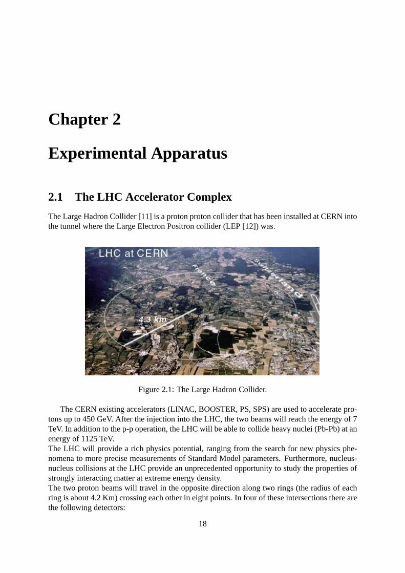
The Large Hadron Collider [11] is a proton proton collider that has been installed at CERN intothe tunnel where the Large Electron Positron collider (LEP [12]) was.
Figure 2.1: The Large Hadron Collider.
The CERN existing accelerators (LINAC, BOOSTER, PS, SPS) are usedto accelerate pro-tons up to 450 GeV. After the injection into the LHC, the two beams will reach the energy of 7TeV. In addition to the p-p operation, the LHC will be able to collide heavy nuclei (Pb-Pb) at anenergy of 1125 TeV.The LHC will provide a rich physics potential, ranging from the search for new physics phe-nomena to more precise measurements of Standard Model parameters. Furthermore, nucleus-nucleus collisions at the LHC provide an unprecedented opportunity to study the properties ofstrongly interacting matter at extreme energy density.The two proton beams will travel in the opposite direction along two rings (the radius of eachring is about 4.2 Km) crossing each other in eight points. In four of these intersections there arethe following detectors:
18

CHAPTER 2. EXPERIMENTAL APPARATUS 19
• ATLAS, A ToroidalLHC ApparatuS
• CMS,CompactMuonSolenoid
• ALICE, A L argeIonCollider Experiment
• LHCb, LargeHadronCollider bphysics
Figure 2.2: System to inject proton beams into the final collider LHC.
The two proton beams will pass through oppositely directed field of 8.38 Tesla. Thesefields are generated by superconducting magnets operating at 1.9 K. The protons will comein roughly cylindrical bunches, few centimeters long and few microns in radius. The distancebetween bunches is 7.5 m, in time 25 ns.In the high luminosityphase (1034cm−2s−1), the twobeams will be made of 2808 bunches of about 1011 protons each. During the initial phase, LHCwill run at a peak lower luminosity of 1033cm−2s−1.The uminosityL of a collider is a parameter of the machine that connects the interaction crosssection (σ) with the number of events per unit time (Ne):
Ne = L σ (2.1)
The luminosity is related to the properties of the collidingbeams and can be expressed interms of the machine parameter:
L = Ff n1n2
4πσxσy(2.2)
where thef is the particle bunch collision frequency,n1 andn2 are the number of particlesper bunch,σx e σy are the parameters which characterise the beam profile in thedirections or-thogonal to the beam andF , equal to 0.9, depends on the crossing angle between the beams.LHC could reach a design luminosity of 1034cm−2s−1: this is important to study processes witha small cross section value.

CHAPTER 2. EXPERIMENTAL APPARATUS 20
2.2 The ATLAS Detector
At the LHC the high interaction rates, radiation doses, particle multiplicities and energies, aswell as the requirements for precision measurements have set new standards for the design ofparticle detectors.ATLAS is a general-purpose detector designed to maximize the physics discovery potential of-fered by the LHC accelerator. Requirements for the detector system [13] have been definedusing a set of processes covering much of the new phenomena which one can hope to observeat the TeV scale. In the following I will focus the attention in describing subdetectors that arefundamental for the reconstruction of the channel with a Z boson produced in association to ab-jet and the Z decaying into two muons of opposite charge.
2.2.1 The coordinate system and nomenclature
The coordinate system and nomenclature used for describingthe detector and the particlesemerging from the p-p collisions are briefly summarised hereas they are used repeatedlythroughout this thesis.The beam direction defines thez-axis and thex− y plane is transverse to the beam direction.The positivex-axis is defined as pointing from the interaction point to thecentre of the LHCring and the positivey-axis is defined as pointing upwards. The side-A of the detector is definedas that with positivez and side-C is that with negativez.
Figure 2.3: Schematic design of the ATLAS detector.

CHAPTER 2. EXPERIMENTAL APPARATUS 21
As it is shown in figure 2.3 the ATLAS has a cylindrical geometry, so it is useful to define acylindrical coordinate system (z,R,φ) in order to measure particles coming from the collision:zis the position in the direction along the beam axis, R is the radius in thex−y plane measuredfrom the nominal interaction point andφ is the azimuthal angle measured around the beamaxis. The relation between R andzcan be expressed using the polar angleθ. The mathematicaldescriptions of these variables are the following:
R=√
x2 +y2 (2.3)
θ = arccosz√
R2 +z2(2.4)
φ = arctanyx
(2.5)
A convenient set of kinematic variables for particles produced in hadronic collisions is thetransverse momentumpT , the rapidityy and the azymuthal angleφ. For a particle with energyE and three momentum~p = {px, py, pz}
px = pT cosφ, py = pT sinφ, pT =√
p2x + p2
y, pz = pl . (2.6)
Since the motion between the parton center of mass frame and the hadron laboratory frameis along the beam direction (~z), variables involving only the transverse components are invariantunder longitudinal boosts. It is thus convenient to write the phase space element in cylindricalcoordinates as
d3~pE
= dpxdpydpz
E= pTdpTdφ
dpz
E(2.7)
Both pT andφ are boost invariant, so isdpzE .
We can also write the phase space element in term of the rapidity variable defined as
y =12
ln(E + pz
E− pz) (2.8)
such as
d3~pE
= pTdpTdφdy (2.9)
The use of boost invariant variables facilitates the description of particle production inhadronic collisions, since these phenomena are approximately boost invariant for not too ex-treme values of rapidity. This fact is particularly simple to understand for high energy scat-tering phenomena, where the incoming hadrons behave as beams of quark and gluons, with agiven distribution in longitudinal momenta and limited transverse momentum. It is clear that,depending upon the energy of the incoming constituents, thesame hard scattering phenomenoncan take place with an effective center of mass (i.e. with a center of mass for the incomingconstituents) that is moving along the collision direction. Experimentally, it is convenient touse the pseudorapidity: the pseudorapidityη is defined as

CHAPTER 2. EXPERIMENTAL APPARATUS 22
η = −ln(tanθ2
) (2.10)
In terms of momenta it can be definied as
η = ln(p+ pl
pT) (2.11)
Being only a function of the angle, pseudorapidity is much easier to measure than rapidity,and it is simple to proof that in the limitp≫ m ,we obtainη = y.
The detector is geometrically divided in three sections:
Barrel: |η | < 1.05
Extended Barrel: 1.05< |η | < 1.4
Endcap:|η | > 1.4
Other variables useful to describe particles emerging fromthe interaction are the tranverseenergyET , the missing transverse energyEmiss
T and the angular distance∆R:
ET = ∑√
p2x + p2
y (2.12)
EmissT =
√(∑ px)2 +(∑ py)2 (2.13)
∆R=√
∆η 2 +∆φ2 (2.14)
where the sum is over all particles originating from the interaction.
2.2.2 Physics requirements
The formidable LHC luminosity and resulting interaction rate are needed because of the smallcross-sections expected for many of the processes mentioned above (see figure 2.4).
However, with an inelastic proton-proton cross-section of80 mb, the LHC will produce atotal rate of 109 inelastic events/s at design luminosity. This presents a serious experimentalchallenge as it implies that every candidate event for new physics will on the average be accom-panied by∼20 inelastic events per bunch crossing.The nature of proton-proton collisions imposes another difficulty: jet production cross-sectiondominate over the rare processes mentioned above, requiring the identification of experimentalsignatures characteristic of the rare physics processes inquestion, such asEmiss
T or secondaryvertices. Identifying such final states for these rare processes imposes further demands onthe particle-identification capabilities of the detector and on the integrated luminosity needed.Viewed in this context, these benchmark physics goals can beturned into a set of general re-quirements for the detector:

CHAPTER 2. EXPERIMENTAL APPARATUS 23
Figure 2.4: Proton-(anti)proton cross sections for several processes as a function of the centerof mass energy.
- a good charged-particle momentum resolution and reconstruction efficiency in the innertracker. For offline tagging ofτ -leptons andb-jets, vertex detectors close to the interac-tion region are required to observe secondary vertices;
- a very good electromagnetic (EM) calorimetry for electronand photon identification andmeasurements;
- a full-coverage hadronic calorimetry for accurate jet andmissing transverse energy mea-surements;
- an high precision muon system that guarantees accurate muon momentum measurementsover a wide range of momenta;
- a very efficient trigger system on high and low transverse-momentum objects (minimumbiasevents) with sufficient background rejection.
ATLAS has been designed in order to satisfy these requeriments.

CHAPTER 2. EXPERIMENTAL APPARATUS 24
The magnetic system, subdetectors and the trigger system are briefly introduced in the followingsections.
2.3 Magnetic System
The magnetic system consists of a central solenoid (CS) that provides a solenoidal field of2 Tesla for the inner detector and three large air-core toroids, two in the end-caps (ECT) andone in the barrel (BT) that generate the magnetic field in the muon spectrometer (see figure 2.5).
Figure 2.5: View of the superconducting air-core toroid magnet system.
The CS creates a solenoidal field with a nominal strength of 2 T at the interaction point.The real field provided by the CS is not uniform inz nor in R direction. The position in frontof the Electromagnetic calorimeter requires a careful minimisation of matter in order to avoidshowering of particles before their enter the calorimeter.
The design of magnetic system was motivated by the need to provide the optimised mag-netic field configuration while minimizing scattering effects.The two end-cap toroids (ECT) are inserted in the barrel toroid (BT) at each end and line upwith the central solenoid. Each of the three toroids consists of eight coils assembled radiallyand symmetrically around the beam axis.Both BT and ECT generate a precise, stable and predictable magnetic field ranging from 3 to8 Tm for the muon spectrometer. This field is produced in the barrel region (|η | ≤ 1.0) bythe BT and in the forward region (1.4≤ |η | ≤ 2.7) by the ECT, while in the transition region(1.0≤ |η | ≤ 1.4), it is produced by a combination of the two.Due to the finite number of coils, the magnetic field provided by the toroids is not perfectly

CHAPTER 2. EXPERIMENTAL APPARATUS 25
toroidal: it presents strong discontinuities in transition regions, as it can be seen in figure 2.6.The lines are drawn in a plane perpendicular to the beam axis in the middle of an end-cap toroidand the range between two consecutive lines is of 0.1 T.
Figure 2.6: Magnetic toroid field map in the transition region, the lines are drawn in a planeperpendicular to the beam axis in the middle of an end-cap toroid.
2.4 Inner Detector
The inner detector (ID) is the innermost part of ATLAS and is designed to reconstruct theproduction and decay points (vertices ) of charged particles as well as their trajectories (seefigure 2.7).It combines high resolution detectors (pixel) at the inner radii, with tracking elements at theouter radii covering the range of|η | < 2.5 and it is placed within a solenoidal magnetic field of2T. The outer radius of the ID cavity is 115 cm and its length is7 m.
The overall layout consists of three different technologies: the pixel detector, at radii be-tween 5 and 15 cm from the interaction region and the silicon strip detector (SCT) at radiibetween 30 and 50 cm (both of which use semiconductor tracking technology) and the transi-tion radiation tracker (TRT) at outer radii.
Performance requirements of the ID include [13]:
• Resolution:σPT /PT = 0.05%PT ⊕1%.
• Tracking efficiency better than 95% over the full coverage for isolated tracks withPT > 5GeV and a fake-track rate≤ 1% of signal rates.

CHAPTER 2. EXPERIMENTAL APPARATUS 26
Figure 2.7: 3D view of the Inner Detector system.
• At least 90% efficiency for reconstructing both primary (PT ≥ 5 GeV) and secondary(PT ≥ 0.5 GeV) electrons. For primary electrons both bremsstrahlung and trigger effi-ciency are taken into account.
• Tagging of b-jets by displaced vertex with an efficiency≥ 40%. This is done with arejection of non b-hadronic jets≥ 50. (At low luminosity, efficiency≥ 50% for taggingb-jets).
• Identification of individual particles in dense jets and of electrons and photons that formsimilar clusters in the EM calorimeter. Combined efficiency of ID and EM calorimeterfor photon identification should be≥ 85%.
Pixel Detector
The pixel detector is the closest to the interaction point. It consists of three layers in the barreland five disks in each end-cap. The system provides three precise measurements over the fullsolid angle (typically three pixel layers are crossed), with the possibility to determine the impactparameter and to identify short-life particles.The required high resolution is provided by 140 millions individual square pixels of 50µm inr −φ and 400µm in z. The pixel detector yields excellent spatial resolution inthe bendingplane of the solenoidal magnetic field, essential for transverse momentum measurement. Theposition along the beam axis is measured with slightly less precision.
SCT
The semi-conductor tracker (SCT) is designed to provide eight precision measurements pertrack to determine momentum, impact parameter and vertex position. It consists of four doublelayers of silicon strips. It has a resolution of 17µm in rφ and 580µm in z, and can resolve 2parallel tracks separated by 200µm or more: this permits to resolve ambiguities in the pattern

CHAPTER 2. EXPERIMENTAL APPARATUS 27
recognition (assigning hits to track in the dense tracking environment).
TRT
The TRT constitutes the outermost part of the ID system. It consists of 36 layers of 4 mmdiameter straw tubes interspaced with a radiator to emit transition radiation (TR) from electrons.The track density is relatively low at large radii giving a number of 36 points per track. Thisinsures good pattern recognition performance.The drift-time measurement gives a spatial resolution of 130 µmper straw as well as a low anda high threshold. Thus, the TRT can discriminate between transition radiation hits that havepassed the high threshold, and tracking hits that have passed the low threshold.
2.5 Calorimeter System
The calorimeter (see figure 2.8) has been designed to providemeasurements of the energy ofelectrons, photons, isolated hadrons and jets as well as missing transverse energy. It is dividedinto an Electromagnetic (EM) Calorimeter and a Hadronic Calorimeter each consisting of abarrel and two end-caps.The Electromagnetic Barrel Calorimeter (EMB) covers the pseudorapidity |η | < 1.475, theElectromagnetic End-Cap Calorimeter (EMEC) covers 1.375< |η | < 3.2, the Hadronic End-Cap Calorimeter (HEC) covers 1.5 < |η | < 3.2, the Forward Calorimeter (FCAL) covers 3.1 <|η | < 4.9, and the Tile Calorimeter (TileCal) covers|η | < 1.7.
Because of its good hermeticity, the calorimeter as a whole provides a reliable measure-ment of the missing transverse energy (Emiss
T ). Together with the Inner detector, the calorimeterprovides a robust particle identification exploiting the fine lateral and good longitudinal seg-mentation.
Electromagnetic Calorimeter
The Electromagnetic Calorimeter is a highly granular lead-liquid argon sampling calorimeterwith accordion-shaped lead absorbers and kapton electrodes. This geometry enables the detec-tor to have a hermetically uniform azimuthal coverage.The eletromagnetic shower develops in lead absorber plates. The absorbers are folded into anaccordion shape and oriented alongR (z in the end-caps) to provide completeφ symmetry with-out azimuthal cracks.The total EM calorimeter presents a∼ 20 radiation lengths in the barrel and in the end-caps re-gion to reduce the error in the energy resolution due to longitudinal fluctuations of high energyshowers due to longitudinal leakage.The particle identification is achieved by a fine longitudinal and lateral segmentation. The EMcalorimeter is longitudinally segmented in three layers plus a pre-shower sampler that correctsthe energy loss in the material in front of the EM.

CHAPTER 2. EXPERIMENTAL APPARATUS 28
Figure 2.8: General layout of the calorimeters showing a good hermeticity.
The design of the electromagnetic calorimeter is driven by the requirements for energy andspatial resolution for the Higgs processes involving decays to electrons or photons for the detec-tion of new gauge bosons (Z′ or W′) decaying to electrons. The dinamical range of electronicsfor the calorimeter extends from a few MeV for electrons fromB-meson decays to a few TeVfor the decay of a heavy vector boson. The ability to identifylow energy electrons can im-prove b-tagging by about 10%. The EM calorimeter is expectedto provide excellent energyresolution,
σE(GeV)
=10%√
E(GeV)⊕0.7%
Hadronic Calorimeters
The hadronic calorimeters cover the pseudorapidity range|η | < 4.9 using three different tech-niques because of the wide spectrum of physics requirementsand differing radiation environ-ments. The hadronic calorimetry in the region|η | < 1.7 (Tile Calorimeter) uses iron absorberswith scintillator plates. This technique offers good performance combined with simple, low-cost construction. At larger rapidity (Forward Calorimeters and End Cap Calorimeters), wherehigher radiation resistance is required, the hadronic calorimetry is based on the use of liquidargon.
The hadronic calorimeters are required to identify and measure the energy and direction ofjets as well as the totalEmiss
T . The required jet-energy resolution depends on the pseudorapidityregion and is given by:

CHAPTER 2. EXPERIMENTAL APPARATUS 29
σE(GeV)
=50%√
E(GeV)⊕3%
for |η | < 3.2 and
σE(GeV)
=100%√E(GeV)
⊕10%
for 3.1< |η | < 4.9Through their ability to measure quantities such as leakageand isolation, the hadronic
calorimeters are well suited to complement the EM calorimeters in electron and photon iden-tification. Because of their total thickness in terms of interaction length ( 11λ ), the hadroniccalorimeters are capable of containing hadronic showers and minimizing punch-throughs intothe muon system.
2.6 Muon System
The Muon Spectrometer forms the outer part of the detector and it is, in terms of volume, thelargest component of the detector. It is designed to detect charged particles exiting the barreland end-cap calorimeters and to measure their momentum in the pseudorapidity range|η | <2.7. The accurate determination of the momenta of muons allows the precise reconstructionof the short-lived particles that decay into muons (particles cointaining b or c quarks). Sincemany of the physics processes of interest involve the production of muons, therefore, the iden-tification of muons provide also an important signature for the event selection (trigger) of theexperiment. In fact the Muon Spectrometer is also designed to trigger on these particles in theregion|η | <2.4.
The conceptual layout of the Muon Spectrometer is shown in figure 2.9: the different tech-nologies employed are indicated. In order to have an accurate measurement of the momentum,independently from the inner detector, the design of the muon spectrometer uses four differentdetector technologies including two types of trigger chambers and two types of high precisiontracking chambers. The muon chambers form three concentriccylindrical layers (each calledstation) at radii around 5, 7.5 and 10 m in the barrel region and cover apseudorapidity range of|η | < 1.0. In the forward region (1.0 < |η | < 2.7), the chambers are arranged in four verticaldisks concentric and perpendicular to the beam axis at distances of 7.4, 10.8, 14 and 21.5 mfrom the interaction point (see figure 2.10).
The precision measurements of the muon momentum in the barrel region are based on thesagitta of three stations in the magnetic field, where the sagitta is defined as the distance fromthe point measured in the middle station to the straight lineconnecting the points in the innerand outer stations.In the end-caps, the situation is different; the magnetic field is present only between the innerand the middle stations, therefore the momentum is determined with a point-angle measure-ment: a point in the inner station and an angle in the combinedmiddle-outer stations.

CHAPTER 2. EXPERIMENTAL APPARATUS 30
Figure 2.9: 3D view of the muon spectrometer showing areas covered by the four differentchamber technologies.
2
4
6
8
10
12 m
00
Radiation shield
MDT chambers
End-captoroid
Barrel toroid coil
Thin gap chambers
Cathode strip chambers
Resistive plate chambers
14161820 21012 468 m
Figure 2.10: R-Z view of one quadrant of the muon spectrometer. High energy muons willtypically traverse at least three stations.

CHAPTER 2. EXPERIMENTAL APPARATUS 31
The driving performance goal is a stand-alone transverse momentum resolution of approx-imately 10% for 1 TeV tracks, which translates into a sagittaof about 500µm, to be measuredwith a resolution of≤ 50 µm. Muon transverse momenta down to a few GeV (∼ 3 GeV, due toenergy loss in the calorimeters) may be measured by the spectrometer alone. Even at the highend of the accessible range (∼ 3 TeV), the stand-alone measurements still provide adequatemomentum resolution and excellent charge identification (see fig. 2.13).
2.6.1 Muon Chamber Types
As discussed in the previous section, the chambers are positioned at three stations along themuon trajectory.Thehigh precision tracking systemcomprises the Monitored Drift Tubes (MDT) and the Cath-ode Strip Chambers (CSC). The precision chambers are required to measure spatial coordinatesin two dimensions and to provide good mass resolution as wellas a good transverse momen-tum resolution in both the low and highPT regions. The performance benchmark, given themagnetic field and the size of the spectrometer, requires a position resolution of 50µm. Thespectrometer is designed such that particles from the interaction vertex traverse always threestations of chambers.The muon trigger systemcomprises the Resistive Plate Chambers (RPC) in the barrel regionand Thin Gap Chambers (TGC) in the forward region. These chambers determine the globalreference time (bunch crossing identification) and the muontrack coordinate in both directions.The trigger system is designed to reduce the LHC interactionrate from about 1 GHz to theforeseen storage rate of about 100 Hz. The trigger chambers must be able to trigger with a welldefinedPT cut-off and to measure the coordinates in the direction orthogonal (φ coordinate) bythe precision chambers with a resolution of 5-10 mm.
Precision chambers
Monitored Drift Tube (MDT) A monitored drift tube (MDT) chamber consists of three orfour layers (amultilayer) of 30 mm diameter cylindrical drift tubes each outfitted with a centralW-Re wire of 50µm (see figure 2.11) on each side of a supporting frame. The MDT chambersperform the precision coordinate measurement in the bending direction of the air-core toroidalmagnet and therefore provide the muon momentum measurement.The four layers chambers are located in the innermost muon detector stations where the back-ground hit rates are the highest. An additional drift-tube layer makes the pattern recognition inthis region more reliable.
The MDTs are operated with a gas mixture of 93% Argon and 7%CO2 at a pressure of 3atm. The tube lengths vary from 70 to 630 cm as a function of chamber position around thedetector. The chambers are positioned orthogonal to ther −z plane (wires parallel to magneticfield lines) in both the barrel and end-cap regions, thus providing a very precise measurementof of the axial coordinate (z) in the barrel and the radial coordinate (r) in the transition and end-cap regions. The MDTs provide a maximum drift time of about 700 ns and a single tube (wire)resolution of 80µm, while the resolution in the bending direction is 40µm. The momentumresolution is shown in figure 2.13.The precision measurement of muons tracks are done everywhere using MDTs except in theinnermost ring of the inner station of the end-cap, where particle fluxes are highest. In this

CHAPTER 2. EXPERIMENTAL APPARATUS 32
Figure 2.11: Schematic view of an MDT module with detail of the tube arrangement in theinlet.
Figure 2.12: Drift path of an ionized particle in a magnetic field.

CHAPTER 2. EXPERIMENTAL APPARATUS 33
region the CSCs are used.
0
2
4
6
8
10
12
10 102
103
pT (GeV)
Con
trib
utio
n to
res
olut
ion
(%)
Wire resolution and autocalibration Chamber alignment Multiple scattering Energy loss fluctuations Total |η| < 1.5
Figure 2.13:∆pT/pT as a function ofpT for muons reconstructed in the barrel region (η ≤ 1.5).
Cathode Strip Chambers (CSC) The CSC are multiwire proportional chambers with bothcathodes segmented, one with the strips perpendicular to the wires providing the precision co-ordinate and the other parallel to the wires providing the transverse coordinate. The positionof the track is obtained by interpolation between the charges induced on neighbouring cathodestrips. The CSC wire signals are not read out.
Each CSC chamber consists of 4 layers. The CSC are operated witha non flammable gasmixture of 80% Argon and 20%CO2 and provide a maximum drift time of 30 ns. An r.m.s timeresolution of 3.6 ns results in a reliable tagging of the beam-crossing..The precision coordinate is obtained by measuring the charge induced on the cathode strips bythe avalanche formed on the anode wire. The cathode strips are oriented orthogonal to the anodewire and are segmented, to obtain a position measurement with a resolution of 60µm per CSCplane. In the non-bending direction the cathode segmentation is coarser leading to a resolutionof 5 mm.The parallel strips provide theφ coordinate. Installed at a distance of seven meters from theinteraction point and 2.0< |η |< 2.7, these muon detectors are built to survive the high radiationenvironment produced by the colliding high-energy protons.
Trigger chambers
Resistive Plate Chambers (RPC) The trigger system in the barrel consists of three concentriccylindrical layers around the beam axis, referred to as the three trigger stations.
The RPC is a gaseous parallel electrode-plate (i.e. no wire) detector. Each of the tworectangular detector layers are read out by two orthogonal series of pick-up strips: theη stripsare parallel to the MDT wires and provide the bending view of the trigger detector, theφ stripsorthogonal to the MDT wires provide the second coordinate measurement which is also requiredfor the offline pattern recognition. The use of the two perpendicular orientations allows the
CHAPTER 2. EXPERIMENTAL APPARATUS 34
measurements of theη andφ coordinates. The RPC combine an adequate spatial resolutionof1 cm with an excellent time resolution of 1 ns.The number of strips (average strip pitch is 3 cm) per chamberis variable: 32, 24, 16 inη andfrom 64 to 160 inφ. When a particle goes through an RPC chamber, the primary ionizationelectrons are multiplied into avalanches by a high electricfield of typically 4.9 kV/mm. Thesignal is read out via a capacitive coupling of strips on bothsides of the chamber.
Thin Gap Chambers (TGC) Thin Gap Chambers (TGC) provide two functions in the end-cap muon spectrometer: the muon trigger capability and the determination of the second, az-imuthal coordinate to complement the measurement of the MDTin the bending direction.
They are very thin multi-wire proportional chambers The peculiarity of TGC comparedto regular MWPC is that cathode-anode spacing is smaller thanthe anode-anode (wire-wire)spacing. This characteristic allows a shorter drift time and an excellent response in time of lessthan 20 ns, which meets the requirement for the identification of bunch crossings at 40 MHz.The TGC are filled with a highly quenching gas mixture of 55%CO2and 45%n-pentaneC5H12.This allows TGC to work in a saturation operation mode with a time resolution of 5 ns and withgood performances in a high particle flux.
2.7 The Trigger and Data Acquisition System
As already discussed, LHC should work at a design luminosityof 1034cm−2s−1 in order to allowthe studies of rare events. This condition will lead to over 23 interactions per bunch crossing.Thus, each second close to 109 interactions occur. Most of these interactions are minimumbiasevents that have a limited interest corresponding to an amount of data of≈ 4×10⁴ Gbytes−1.Therefore it is necessary to select interesting data in order to register only the interesting portionof the total amount of data coming from the collision. To satisfy this request, a trigger systemand a data aquisition system (DAQ) (see figure 2.14) have beendesigned with the challengingrole of selecting bunch crossings containing interesting events by reducing the data rate from40 MHz (collision rate) to 100-200 Hz.
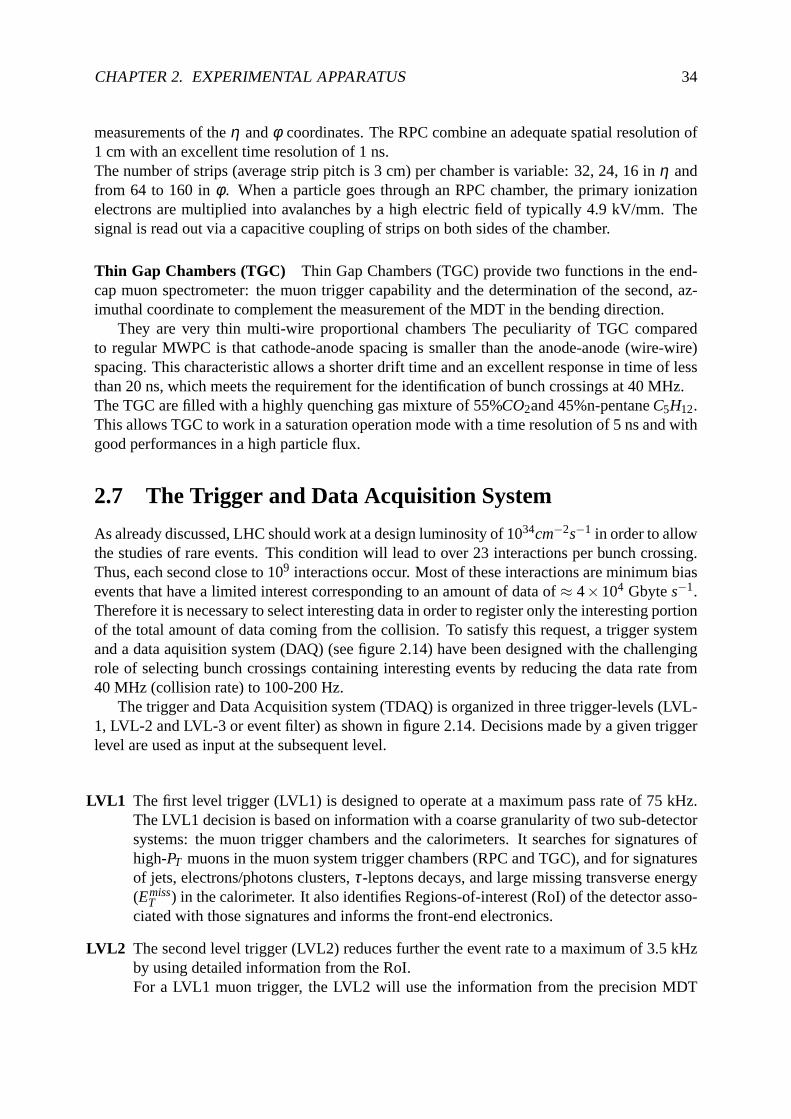
The trigger and Data Acquisition system (TDAQ) is organizedin three trigger-levels (LVL-1, LVL-2 and LVL-3 or event filter) as shown in figure 2.14. Decisions made by a given triggerlevel are used as input at the subsequent level.
LVL1 The first level trigger (LVL1) is designed to operate at a maximum pass rate of 75 kHz.The LVL1 decision is based on information with a coarse granularity of two sub-detectorsystems: the muon trigger chambers and the calorimeters. Itsearches for signatures ofhigh-PT muons in the muon system trigger chambers (RPC and TGC), and forsignaturesof jets, electrons/photons clusters,τ -leptons decays, and large missing transverse energy(Emiss
T ) in the calorimeter. It also identifies Regions-of-interest(RoI) of the detector asso-ciated with those signatures and informs the front-end electronics.
LVL2 The second level trigger (LVL2) reduces further the event rate to a maximum of 3.5 kHzby using detailed information from the RoI.For a LVL1 muon trigger, the LVL2 will use the information from the precision MDT
CHAPTER 2. EXPERIMENTAL APPARATUS 35
LVL2
LVL1
Rate [Hz]
40 × 106
104-105
CALO MUON TRACKING
Readout / Event Building
102-103
pipeline memories
MUX MUX MUX
derandomizing buffers
multiplex data
digital buffer memories
101-102
~ 2 µs(fixed)
~ 1-10 ms(variable)
Data Storage
Latency
~1-10 GB/s
~10-100 MB/s
LVL3processor
farm
Switch-farm interface
Figure 2.14: The trigger levels and DAQ.
chambers to improve the muon momentum estimate, which allows a tighter cut on thisquantity. For a LVL1 calorimeter trigger, the LVL2 has access to the full detector gran-ularity, and has in addition the possibility to require a match with a track reconstructedin the inner detector. The LVL2 has an event dependent latency, which varies from 1ms for simple events to about 10 ms for complicated events. For events accepted by theLVL2, the data fragments stored in the RoI are collected by theso-called Event Builderand written into the Full Event Buffers. The event builder system assembles and ships tothe LVL-3 trigger the full event data of all events accepted by the LVL-2. The averageevent processing time at this level is about 40 ms per event.
LVL3 The third trigger stage is called LVL3 and uses up to date detector information includingmagnetic field maps, calibration results and full granularity and precision of the calorime-ter, muon system and ID to further reduce the event rate. The LVL3 can use complexoffline algorithms like track reconstruction, vertex finding, etc., because it has access tothe complete event. The stored data is reconstructed to yield quantities like tracks, energyclusters, jets, missing transverse energy, secondary decay vertices, etc. These quantitiesare subject to various physics selection criteria in offlineanalyses too, for example tomaximise the discovery potential for the Higgs particle. For the maximum trigger rate of100-200 Hz the average event processing time will be of orderfour seconds.
All the data flow between various front-end electronics and different trigger levels is handled
CHAPTER 2. EXPERIMENTAL APPARATUS 36
by the Data Acquisition (DAQ) system. It stores the information from all detectors in pipelinedmemories while decision is being made (latency) by the trigger system. The DAQ also providesconfiguration, control and monitoring of the detector during data-taking.
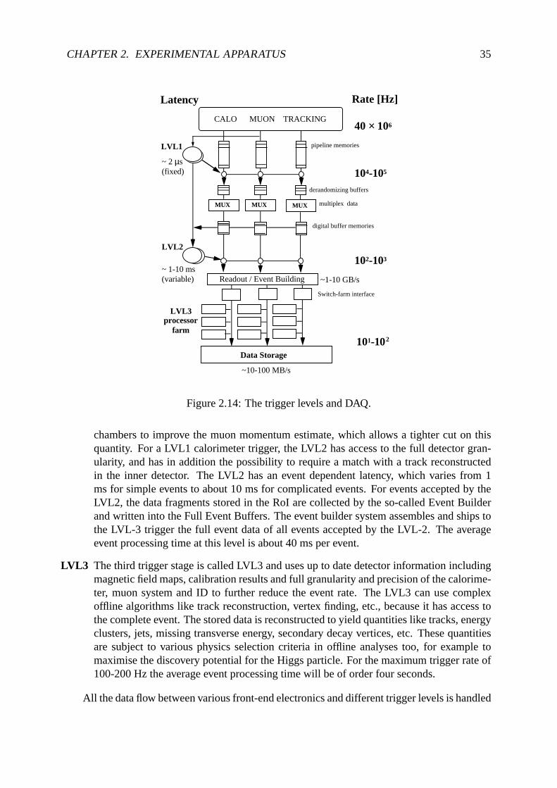
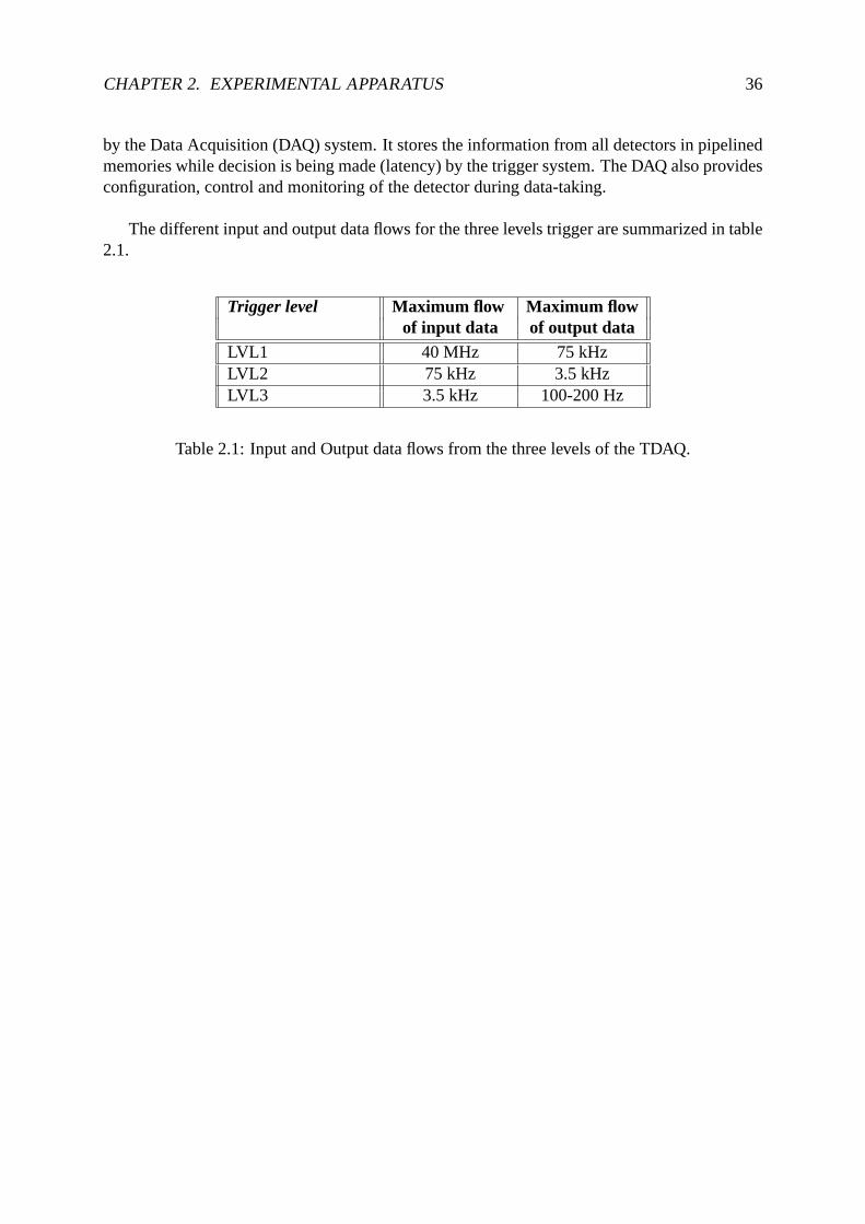
The different input and output data flows for the three levelstrigger are summarized in table2.1.
Trigger level Maximum flow Maximum flowof input data of output data
LVL1 40 MHz 75 kHzLVL2 75 kHz 3.5 kHzLVL3 3.5 kHz 100-200 Hz
Table 2.1: Input and Output data flows from the three levels ofthe TDAQ.
Chapter 3
Software tools
In order to provide realistic predictions for the experimental capabilities of detecting physicalprocesses, the simulation of the detector response interfaced to a Monte Carlo generator is cru-cial.The whole software is implemented in a global framework written in C++ programming lan-guage, called ATHENA [22]. This framework is a working environment under which the usercan apply his own analysis algorithm to select the signal andthe backgrounds he is interested in.The ATLAS software framework is continously updated to allow developers to insert new codeand amend bugs. Periodically the whole software is ’released’ and given a Release Number.This is a group of three integers separated by dots, where thefirst number is the major release,the second indicates developer release, and the third indicates minor changes. A summary ofall releases and their properties can be found in [23].
A detailed description of the performances of the detector and its response to all the inter-esting physics processes before the start up of LHC requiresthe use of three separate softwaremodules that can be run either separately or in sequence under the ATHENA infrastructure:
• event generation ;
• detector simulation;
• digitization.
The results of this thesis have been obtained using the ATHENA framework. Different re-leases have been used. They will be specified for each study decribed in the following chapters.
Event generation The first step of the event generation phase is implemented within ATHENAusing physics event generators.Generally the generators simulate the collisions of various particle species (protons, electrons,...) at a given center of mass energy (see section 3.1). Generators also simulate particles emerg-ing from the interaction region. A physics event generator produces lists of particles. The inputto the generator is usually in the form of beam energy, tablesof decay probabilities, specificparticle reactions, and specific final state particles. The output is a list of events which serveas input to the simulation. Each particle is parameterized by particle-type, initial vertex, initial
37
CHAPTER 3. SOFTWARE TOOLS 38
and final four-momentum vectors. Event generators are frequently updated to keep up with thelatest theoretical insights. In the case of LHC phenomenology, calculations must include QCDuncertainties due to the parton distribution functions andthe hadronisation.
Detector simulation Detector simulation is the simulated response of the detector to particlesgenerated in the interactions and their decay products.There is not an unique way of implementing the detector simulation. The accuracy by whichthe detector performance need to be simulated strongly depends on the purpose of the analysis.Two types of detector simulation exist in the Atlas softwareframework: Geant4 full detectorsimulation [30] (full simulationsee section 3.2) andAtl f ast fast detector simulation [39] (fastsimulationsee section 3.3).The former is based on complete detector material description including the best possible de-tails. The latter does not consider detector materials in details; it only smears the kinematics ofthe MC particles according to the expected detector performance.Full simulation is desiderable to study detector performances and systematic uncertainties origi-nating from the intrinsically limited detector resolution, but it is an intensive computing processthat can take up to∼ 30 minutes per event, using a large amount of memory, CPU and diskspace.Fast simulation, on the other hand, takes a small fraction ofa second per event. For some feasi-bility studies that require a large amount of statistics, a simple parameterisation of the smearingof the particle observable parameters can be sufficient. This means that for this kind of studiesalso the fast simulation can be used.To make final conclusions from the simulation studies, oftenone needs to combine the resultscoming from full and fast simulations.
Digitization The digitization step is the final phase, where the depositedenergies in the vari-ous detector elements are recorded, collected and reprocessed in order to simulate the electronicoutput from the detector. The digitization stage includes simulation of physics effects specificto each type of detector and of the front-end electronics response and of noise. The output of thedigitization is written into Raw Data Objects (RDO) to be used by the reconstruction programs.These reconstruction programs are the same that will be usedonce the experiment will start totake data.
Figure 3.1 shows how the simulated raw data, Raw Data Object (RDO), is produced fromthe generated Monte Carlo (MC or Truth) events. In this schemealso the data flow produced bythe experiment is presented. ATLAS data will be recorded as asequence of bytes that must beconverted by the ByteStream ConversionSvc into RDO in order to be used by the reconstructionprograms.
Reconstruction In order to convert this raw information to more fundamentalphysics objectsthe recorded events are processed through a set of computer algorithms that constitue the recon-struction process. This process will be discussed in more detail in section 3.2.2, neverthless insummary here is a schematical division of such a process intothree main stages:
• data from each subdetector are reconstructed in stand-alone mode;

CHAPTER 3. SOFTWARE TOOLS 39
Figure 3.1: Schematic diagram showing the flow of MC data through simulation and digitisationprocess.
• informations from all sub detectors are combined to identify the observable objects suchas tracks, muons, jets etc.;
• informations from different observable objects are combined into reconstruction algo-rithms for selecting the signal and rejecting backgrounds.
3.1 Monte Carlo Events Generators
Events produced by Monte Carlo (MC) generators are essential tools of physics analysis. Asalready discussed, to make a realistic estimation of feasibility for future analysis, to comparedata with theoretical predictions, or to understand the detector performance in detail, the detec-tor response to MC events need to be simulated.There are many Monte Carlo generators in particle physics, the most widely used arePYTHIA[24], HERWIG[26], ALPGEN[27], SHERPA[25] andMC@NLO[28], which are general pur-pose Monte Carlo. They have been tested in many particle physics experiments and are conti-nously updated to include new process and the most recent calculations.Each Monte Carlo generator is interfaced to a library called LHAPDF [58] containing infor-mations about different parton distribution functions(PDF) sets. This interface provides thepossibility to choose among different PDF sets in order to generate data samples. A more de-tailed description on PDF and kinematic range of validity will be discussed in section 3.1.2.
In this analysis Monte Carlo event generators are used in a variety of ways, from findingcharacteristic spectra for variables associated withZ boson and b quarks or b-jet to finding pre-dictions for the cross section of signal and background processes.PYTHIAandSHERPAeventgenerators interfaced to the ATHENA framework have been used.

CHAPTER 3. SOFTWARE TOOLS 40
3.1.1 The QCD model
A general purpose Monte Carlo generator should contain a simulation of several physics as-pects. After the two beam particles come in towards each other, we can try to follow the evolu-tion of an event in timing order arranging it as follows:
• Initial State Radiation:One shower initiator parton from each beam starts off a sequence of branchings , suchasq → qg, which build up an initial state shower according to QCD calculations. Thequarks can also radiate photons according to QED.
• Hard Process:One incoming parton of the two showers enters the hard process. The hard process mayproduce a set of short lived resonances, like theZ gauge boson, whose decay to partonshas to be considered in close association with the hard process itself.
• Final State Radiation:The outgoing partons generated in the final state of the Hard Process may branch, justlike the incoming did, to build up final state showers.
• Hadronisation:The QCD confinement mechanism ensures that the outgoing quarks and gluons are notobservable. This mechanism forces all coloured particles to bind together in order to formcolour neutral hadrons, which can be experimentally detected.
• Underlying Event:Besides the hard process considered above, further interactions may occur between theother partons of the two incoming hadrons. Tipically these are soft interactions generatinglow pT particles. In addition, in high-luminosity colliders, it is possible to have severalcollisions between beam particles in one and the same beam crossing, i.e. pile-up events,which further act to build up the general particle production activity that is to be observedby detectors.
• Particle decays:Many of the produced hadrons are unstable and decay further.
A sketch of these steps is the one in figure 3.2.
In the following sections I will go through these aspects notin the same order as givenabove, but rather in the order in which they appear in the program execution, i. e. starting withthe hard process.
Hard Process
The Hard Process yields the physical signal: two partons from the two colliding hadrons interactto produce the final state partons.The inclusive cross sections (σh
a,b) for hard production processes are calculable in terms of the

CHAPTER 3. SOFTWARE TOOLS 41
Figure 3.2: Schematic drawing of an interaction involving quarks. First the hard-scatteringoccurs which could include some initial and final state radiation (1). In this case a decay oftwo photons (wavy lines) to two pairs of quarks (straight lines) is shown. Then the Final StateRadiation (FSR) process occurs (2): many gluons (spring like lines) can be emitted which can inturn decay to quark-antiquark pairs. This process occurs until the energy scale of each parton isclose tot0. The non-perturbative hadronisation process then occurs (3) which turns the partonsinto hadrons. The latter can decay into a series of final stateparticles (4) which are measuredby the detector (5). Finally objects such as jets are reconstructed from what is observed in thedetector (6). In this case four jets would be observed.
so called QCD-improved parton model formula 1.16.For a more detailed description of the Hard Process I refer tosection 1.3.2.
Initial and Final State Radiation
The Initial andFinal State QCD Radiation(ISR and FSR) process, also called fragmentation,are the processes whereby the partons create many more partons. This process is illustrated inthe part (1) and (2) of figure 3.2. A quark can emit a gluon,a gluon can emit another gluon orconvert into a quark-antiquark pair. This process continues until the virtual masses squared ofthe partons are of the order of the infrared cut-off scale,t0, taken to be of the order of 1GeV2 .Fragmentation models focus on the calculation of approximate results of parton showeringwhere the enhanced terms, such as soft or collinear parton emission from the primary par-ton, are taken into account for all orders of the perturbative expansion in terms dependent onαs. The parton shower models represent an approximate perturbative treatment of QCD dy-namics at scales larger thant0. The implementation of fragmentation models in Monte Carlosimulations mostly use Sudakov form factors. These form factors determine the probability ofevolving from the initial scalet to the shower cut-off scalet0. Each parton species has its ownform factor. For more details see [9,10].
Summarizing at high energy scale the fragmentation ofqq in high energy partons (gluonsandqq couple) is described byperturbative QCD. At small energy scale the soft gluon radiation(or radiation from gluon of lowpT) must be described through fenomenological models (nonperturbative QCD).
CHAPTER 3. SOFTWARE TOOLS 42
Underlying Event
The presence of a significant amount of soft interactions between the colliding hadrons (beam-beam remnant interactions), possible multiple parton interactions and gluon radiation from theinitial partons before the hard interaction (initial stateradiation) complicate things even further.These additional processes are collectively known as theunderlying event. From an experi-mental point of view, in a hadron-hadron interaction with jets in the final state, the underlyingevent is all the activity accompanying the two hard scattered outgoing jets. The underlyingevent, along with the finite detector resolution, leads to the fact that it is not possible to unam-biguously determine, even in Monte Carlo simulation, which hadrons came from which initialparton, i.e. which hadrons belong to which parton jet. It is impossible to separate these twocomponents due to the lack of knowledge in modeling the underlying jet structure.The typical approach to modelize the UE is to rely on particleand energy densities inη −φregions that are well separated with respect to the highpT objects (for example jets). In showerMonte Carlo model, the underlying event is a component of the process simulation that acts atthe end of the showering and before the hadronisation, in order to complete the process descrip-tion taking into account soft components (hadronic remnants and multiple interaction).Huge progress in the phenomenological study of the underlying event in jet events has beenachieved by the CDF experiment at the Tevatron [15, 16], usingthe multiplicity and transversemomentum spectra of charged tracks in different regions of the azimuth-pseudorapidity space,defined with respect to the direction of the leading jet. Regions that receive energy flow contri-butions mostly by the underlying event have been identified.
Hadronisation
After the fragmentation, the low-momentum-transfer, long-distance regime is entered, in whichnon-perturbative effects become important. The most important of these effects is hadronisa-tion which converts the partons into the observed hadrons (part (3) of figure 3.2). Most mod-els of these phenomena, when implemented in Monte Carlo simulations, assume that the twoprocesses, fragmentation and hadronisation, occur in sequence and can thus be treated indepen-dently [9].In principle, the shower cut-off,t0, is an arbitrary parameter, uncorrelated with the hadroni-sation process but whent0 is increased, the parton shower is terminated earlier and there arefewer partons to hadronise. Thus the hadronisation models should have a parametert0 whoseeffect cancels out when the parton shower model and the hadronisation model are combined. Inpracticet0 is tuned such that the final number of hadrons agrees with experimental observation.
Particle decays
Not all the particles produced are stable, some of them have ashort lifetime. The particleswith a life time shorter than a value fixed in the Monte Carlo generator (default is typically1.0×10−8 s) are forced to decay. All other particles are considered stable by the MC generator.Unstable particles with a longer lifetime are forced to decay in the detector simulation as it willbe discussed in section 3.2.1.

CHAPTER 3. SOFTWARE TOOLS 43
3.1.2 Parton Density Function (PDF)
The calculation of the production cross sections at hadron colliders for both interesting physicsprocesses and their backgrounds relies upon a knowledge of the distribution of the momentumfractionx of the partons (quarks and gluons). If the understanding of the perturbative correc-tions to the hard scattering cross section of eq. 1.16 is in good shape, the uncertainty on thePDFs can limit the accuracy of the theoretical predictions.In order to evaluate PDF uncertainties on some observables distributions or on cross sectionprediction, is it possible to generate different data sample using different PDF sets. Here I willbriefly discuss how PDF are determined and which sets are the most common used nowadays.
Perturbative QCD does not provide the PDF’s analytic dependence as a funcion ofx (whichhas a non perturbative origin) but through the DGLAP equations [7] it provides the evolutionfrom a fixed scaleQ2
0 to a givenQ2.The common way to obtain PDF’s as a function ofx andQ2 is to parametrize the quark andgluon density functions in order to perform a global fit of experimental data.All global analyses use a generic form for the parametrization of both the quark and gluondistributions at some reference valueQ0:
F(x,Q0) = A0xA1(1−x)A2P(x;A3, ...) (3.1)
The reference valueQ0 is usually chosen in the range 1−2 GeV.The first two factors, in general, are not sufficient to describe either quark or gluon distributions.The termP(x;A3, ...) is a suitably chosen smooth function, depending on one or more param-eters, that adds more flexibility to the PDF parametrization. In general, both the number offree parameters and the functional form can have an influenceon the global fit. No unanimousagreement is anyway found on such parameterisations and on the number of free parameters.The current PDF sets are derived from global fits to the available data, which include deepinelastic scattering measurements at HERA and at fixed targetexperiments, Drell Yan mea-surements and the Tevatron data on the inclusive jets production and the W charge asymmetry.Many different groups (CTEQ [50], MRST [51,52], ZEUS [53], H1 [59]) work to provide PDFsets and an estimation of the corresponding errors. The differences among the results are due tothe different experimental inputs and treatment of the theoretical and experimental uncertaintiesentering the global fit. The theoretical uncertainties are related both to the parameterisation attheQ2
0 scale and to the perturbative part (missing orders and approximations). The experimen-tal uncertainties include statistical and systematic errors on the input data and the correlationsamong them. The central values of the PDF’s parameters correspond to the best fit; they areassociated with uncertainties which are conventionally computed along the eigenvectors of thecovariance matrix. In this way the error band for a given PDF set is computed and the uncer-tainty is then propagated to the variable under study. For a more exhaustive treatment see [10].The newest PDFs, in most cases, provide the most accurate description of the world data andshould be utilized in preference to older PDF sets.

CHAPTER 3. SOFTWARE TOOLS 44
Figure 3.3: Left) TheQ2− x kinematic plane for the LHC and previous experiments. Right)PDF’s distributions atQ2 = 10,000GeV2 obtained from CTEQ6.5M set.
Hard process and Parton Density Function at LHC
I showed in section 1.3.2 that the collision between two hadrons (two protons at the LHC) canbe described as an interaction between two partons that constitute the hadrons (see figure 1.8).From the kinematic planeQ2 vs x in the left part of figure 3.3 it is visible that at the LHC thevery low-x region will be accessible at the electroweak scale and the very high one at the TeVscale. At LEADING ORDER (LO) Z production occurs through theqq→ Z process (Q∼ 100GeV). The momentum fraction is given for each parton byx1,2 = MZ√
s e±y, beingMZ the center
of mass energy of the hard partonic process and√
s the center of mass energy of the reaction(14 TeV).From the kinematic plane in figure 3.3 it can be seen that at central rapidities the partons havesmall x, x1 ∼ x2 ∼ 0.005; moving away from the central region they take higher or lower x,always remaining within the range 10−4 < x < 0.1 for measurable values of rapidity|y| < 2.5.ForQ∼ 100 GeV the gluon distribution is dominant atx values of less than 0.1 with the valencequark distributions dominant at higherx. The scattering happens between sea quarks; at suchhigh scalesQ2 = M2 ∼10,000GeV2 the gluon dominates (see figure 3.3, right) the sea quarksare mainly generated via gluon splittingg→ qq.
One of the major influences of the HERA data has been to steepen the gluon distribution atlow x.
CHAPTER 3. SOFTWARE TOOLS 45
3.1.3 Generator parameters
Many parameters are dependent on experimental observationmeasured rather than analyticalexpression and there are uncertainties on those variables.QCD processes are generally sensi-tive to arbitrary choice of scales; sub-processes that accompany hard scattering usually involvenon-perturbative QCD processes that require parameterisedmodelling (see discussion in sec-tion 3.1.2). In this section I summarise these issues together with the values selected for eachgenerator used to produce signal and background events.The following parameters were used common to all generators:
• αem = 1137.04;
• GF = 1.1663910−5GeV−2;
• MZ = 91.19 GeV,ΓMZ = 2.495 GeV;
• MW = 80.42 GeV,ΓMW = 2.124 GeV;
• sin2θW = 0.232;
• Mt = 175 GeV.
To generate samples used in the analysis performed with the fully simulated sample, the lat-est parton distribution set for leading-order generators from the CTEQ collaboration, CTEQ6L[50] have been used. This includes latest data from experiments at HERA [53] and Tevatron foran improved parameterisation.
Samples used for the analysis with the fast simulation have been generated using differentPDF sets in order to compare distributions, as it will be discussed in more detail in chapter 4.
All the samples used for the analysis (both for full and fast simulation studies) do not includeevents with more than one proton proton collision per bunch crossing (pile up events). This isreasonable for a luminosity of less than 1033 cm−2 s−1 sufficient for a first measurement of theprocess studied in this thesis: pp→ Z(µµ) + b jet + X (where X states for everything in thefinal state produced in association to the leading process).
3.2 The Full detector simulation and reconstruction
A detector simulation is crucial for understanding detector acceptances and in many cases formodeling backgrounds. The ATLAS full simulation parameterizes the detector geometry andmaterial using Geant4 [30]. The kinematics of physical processes are reproduced to a certainorder of calculation by a Monte Carlo generator program (see section 3.1). As already describedthe generator gives a set of four-vectors that are smeared bythe detector simulation. The sim-ulation produces data banks from each subdetector identical to those from collision data, andthe simulated data are analysed using the same code as the collision data. The digitised (real orsimulated) event data are read in by theReconstructionsoftware which identifies particles andmeasures their energies and momenta.

CHAPTER 3. SOFTWARE TOOLS 46
3.2.1 GEANT4 Simulation
Geant4 [30] is a common tool used in high energy physics to simulate the particle propagationthrough the detector and particle interaction with active and passive materials. It is based on anobject oriented architecture, implemented using C++. Geant4 takes into account a large numberof physics processes of interaction between the particles and the detector. Firstly it displacesthe primary vertex position to take into account the finite size of the beam overlap region,then itsimulates the energy loss due to dead material inside the detector and saves into stored objectsthe energy deposit in the active detector elements.The simulation requires a precise geometrical descriptionof the detector components includingthe materials used in the manufacture, as well as the magnetic field maps. Detector geometrydescriptions are stored in a database and retrieved by the simulation jobs. Geant4 creates a sim-ulated detector in memory based on the description and then simulates the interaction of inputparticles with the detector.Features required for the detector simulation were identified and results have been validatedwith test-beam data [31], which provided tuning of the relevant parameters. Validation withtest-beam results shows that in almost all cases, comparison with the test-beam data are in verygood agreement, normally at the level of 1% or better [32].The precise description of the detector used in simulation and reconstruction is an important is-sue affecting the quality of calibration. Although implementation of the detailed detector effectsand production efforts has been successful, full detector simulation is one of the most resourceconsuming processes in producing MC based data and significant optimisation is desirable.
3.2.2 Offline reconstruction
The events recorded after the detector simulation program are kept in a raw format (RDO)which contains the digitized information from detector sub-systems like the hits in the track-ing and muon systems and the digitized counts in the calorimeter cells. In order to convertthis raw information to more fundamental physics objects like electrons, and provide usefulkinematic as well as quality information, the recorded events are processed through a set ofcomputer algorithms called the offline event reconstruction. In order to study the reconstructionperformances, the same algorithms which are under development for the real data are appliedon simulated events.The analysis shown in this thesis was realized using reconstruction done within Athena releases12.0.4 and 12.0.6. A description of releases and changes that can account moving from onerelease into another, can be found in [23].In the next few sections, I will give more detailed accounts on how the offline reconstruction isperformed and I will refere to observables defined in section2.2.1 such as transverse momen-tum, rapidity and angular distance.
Inner detector tracks
Different stategies have been developed to reconstruct tracks in the inner detector, here I willdiscussed the most common used. Track reconstruction can belogically sub-divided into threestages:

CHAPTER 3. SOFTWARE TOOLS 47
1. A pre-processing stage, in which the raw data from the pixel and SCT detectors are con-verted into clusters and the TRT raw timing information is turned into calibrated driftcircles. The SCT clusters are transformed into space-points.
2. The default track-finding exploits the high granularity of the pixel and SCT detectors tofind prompt tracks originating from the vicinity of the interaction region. First, trackseeds are formed from a combination of space-points in the three pixel layers and the firstSCT layer. These seeds are then extended throughout the SCT to form track candidates.Next, these candidates are fitted, outlier clusters are removed, ambiguities in the cluster-to-track association are resolved, and fake tracks are rejected. The selected tracks arethen extended into the TRT to associate drift-circle information in a road around theextrapolation and to resolve the left-right ambiguities. Finally, the extended tracks arerefitted with the full information of all three detectors andthe quality of the refitted tracksis compared to the silicon-only track candidates.
3. A post-processing stage, in which a primary-vertex finderis used to reconstruct primaryvertices.
This strategy is expected to give very high detection efficiency over the full detector accep-tance,|η | < 2.5.
Calorimeter Tower and Topological Cluster
Calorimeter Towers are built from all calorimeter cells contained in a region of(∆η ×∆φ) ofsize equal to(0.1×0.1). Topological Clusters are built according to criteria that identify signifi-cant energy deposits in topologically connected cells. In particular, cells with> 4σ significance(σ being the standard deviation of fluctuation due to noise) aretaken as seeds and neighbour-ing cells with> 2σ significance are clustered to form energy blobs with a three-dimensionaltopology.
Jets
Jet algorithms are used to group the final state hadrons into jets whose properties are as closeas possible to the initial parton carachteristics. We must distinguish between the so calledTruthJetsandReconstructed Jets. These definitions depend from the input of the algorithm: ifthe jetclustering algorithm run on ”truth” particles (generated from the Monte Carlo program) insidethe detector acceptance, excluding neutrinos and muons, the jets will be calledTruth Jets, whileif the algorithm run over calorimeter towers or topologicalClusters (defined in the previousparagraph) we will refer toReconstructed Jets.
The comparison between the first and the second kind of jets will be a crucial tool in orderto disentangle detector and physics effects.
Two main classes of jet algorithms have been used: theConeandkT [36] algorithms. Thefirst class, the most widely used, looks at the energy deposited in the towers of the calorimeterand define all particles within a physical cone of fixed size tobelong to the same jet. The dif-ferent cone algorithms differ in the method used to find the final cones, in the size of the cones,or in the way of dealing with cones which overlap. This is the class of algorithms which isdiscussed below.

CHAPTER 3. SOFTWARE TOOLS 48
The second class of algorithms defines jets in terms of towerswhich are not close to each otherfrom a spatial point of view but are close to each other inkT . kT is proportional to the relativetransverse momentum between two particles.Historically, cone algorithms have been used in hadron colliders, due to concerns about speed,especially at the trigger level, and of large systematic effects in busy multi-jet environments.Fast implementations of thekT algorithm [37], as well as detailed studies at the Tevatron per-forming precision measurements with the algorithm [38] need detailed comparisons of thekT
algorithm with cone-based ones at the LHC.
The offline reconstruction algorithms take as input anyET ordered list of calorimeter objects(cells, towers or clusters). The jet reconstruction consists of the following steps:
• Removal of negative energy towers (or clusters) by combiningthem with adjacent ones.A list of proto-jets is also constructed using a simple pre-clustering algorithm.
• Removal of proto-jets with transverse energy smaller than a given threshold.
• Running of a jet finding algorithm (cone or kT algorithm) using seeds position defined tobe between proto-jets above a given threshold (default isET > 2 GeV).
• Jet calibration.
• Removal of reconstructed jets below a given transverse energy (default isET > 10GeV).
Jets labelling and tagging
Jets originating from the hadronisation of b quarks can be tagged by exploiting the high massand relatively long lifetime of B hadrons. The average lifetime of the most commonly occurringhadrons containing a b quark such asB+,B0,BS (∼ 1.5 ps), is long enough to allow to a 10 GeVB meson to cover a distance of the order 1 mm before decay. In general the tracks of chargedparticles decaying from these hadrons have large impact parameters with respect to the primaryvertex, and a reconstructable secondary vertex. Typically, jets originating from the hadroniza-tion of b quarks contain 5 - 10 tracks,with about half of them coming directly from the B mesondecay. Therefore one can extrapolate the track measurements from the inner detector to identifythe existence of a secondary vertex or evaluate impact parameters of the tracks with respect tothe primary vertex.To evaluate the likelihood of a given jet to contain a B hadron, the track significance is calcu-lated for each track by taking the ratio of the distance of closest approach to the primary vertex,d0, and the error on the measurementσd0 . Since the resolution in the x-y plane is an order ofmagnitude finer compared to the resolution in the z direction(tens of microns against hundredsof microns),d0 is measured in the transverse plane only (in which case it maybe denoted asa0) although one could obtain more information from includingthe longitudinal impact param-eter (denoted asz0). In fact an important improvement of the performances of the b-taggingalgorithm can be expected by combining thelongitudinal significancewith the transverseone:this algorithm is called the IP3D b-tagging algorithm. The distribution of track significance forlight jets and b-jets are used to construct the likelihood functionPu andPb and finally, a weightis given to the jet [45,46]:

CHAPTER 3. SOFTWARE TOOLS 49
w jet = ∑i∈ jet
ln
[Pb(
ai0
σ ia0
,zi0
σ iz0
)/(Pu(ai
0
σ ia0
,zi0
σ iz0
))
]. (3.2)
The power of the IP3D b-tagging method can be significantly improved by using additionalinformations on the presence or absence of a secondary vertex in the jet. The algorithm usingsecondary vertex is commonly called SV1.
In order to evaluate the goodness of this algorithm, it is possible to define theb-taggingefficiency, themistag probabilityand thec, τ , light jets rejection:
• b-tagging efficiency: is the probability of a b-jet to be tagged as a b-jet.
• mistag probability : is the probability that a given non b-jet is tagged ad a b-jet. Thisvaries as a function of jetpT andη . It also depends on whether the jet containsc quarkor τ lepton.
• rejection: is the inverse of the mistag probability.
It has been proved that the use of both method (IP3D+SV1) can increase the rejection oflight jets significantly, though it was also shown that the method has strong dependence on thetrack reconstruction algorithm and validation of its performance may require an extensive studywith real data [45].In this analysis, the b-tagging algorithm used is the one that makes use of the 3D impact param-eter and secondary-vertex reconstruction, (IP3D+SV1). The distribution of the weight is shownin figure 3.4 separately for light, c and b-jets.
3D impact parameter + secondary-vertex weight-20 -10 0 10 20 30 40
Arb
itrar
y un
its
-610
-510
-410
-310
-210
-110 b-jetsc-jetsLight jets
ATLAS
Figure 3.4: Jetb-tagging weight distribution forb-jets,c-jets and light jets corresponding to theIP3D+SV1 tagging algorithm.

CHAPTER 3. SOFTWARE TOOLS 50
Muons
Muon reconstruction can be done using three different strategies:
• Standalone Muons,
• Combined Muons,
• Calo-tagged Muons.
The differences among them depending on which detector is involved in.Thestandalonereconstruction is the direct approach to reconstruct standalone muons by find-ing tracks in the muon spectrometer, correcting for the energy loss in the calorimeters and thenextrapolating these towards the beam line. Thecombinedmuons are found by matching stan-dalone muons to nearby inner detector tracks and then combining the measurements from thetwo systems.
Multiple independent algorithms have been developed to implement each of these strate-gies and the current baseline reconstruction includes two algorithms for each of the first twostrategies. Here I briefly describe the algorithms that are included in this reconstruction. Thealgorithms are grouped into families such that each family includes one algorithm for each strat-egy. The output data intended for use in physics analysis includes two collections of muons,one for each family, in each processed event. I refer to the collections (and families) by thenames of the corresponding combined algorithms: Staco [35]and Muid [34].
Standalone muons Most of the muons, including those of best quality, are reconstructed byindependently finding tracks in the inner detector and muon spectrometer and then combiningthese tracks. The standalone reconstruction has two major steps: first build track segments ineach of the three muon stations and then link the segments to form tracks. The Staco-familyalgorithm that finds the spectrometer tracks and extrapolates them to the beam line is calledMuonboy [35]. On the Muid side, Moore [33] is used to find the tracks and the first stage ofMuid performs the inward extrapolation.
The extrapolation must account for multiple scattering andenergy loss including that in thecalorimeter. Muonboy assigns energy loss based on the material crossed in the calorimeter.Muid additionally makes use of the calorimeter energy measurements if they are significantlylarger than the most likely value and the muon appears to be isolated.
The standalone spectrometer tracks can also be used alone toidentify muons in regions be-yond the coverage of the inner detector (2.5 < |η | < 2.7), recover muons for which the combi-nation fails and as a check of inner detector performance. Very low momentum muons (around afew GeV) may be difficult to reconstruct because they do not penetrate to the outermost stations.
Combined muons Both of the muon combination algorithms, Staco and Muid, match themuon-spectrometer tracks with inner-detector tracks to identify combined muons. The chi-square, defined as the difference between outer and inner track vectors weighted by their com-bined covariance matrix:
χ2match= (TMS −TID )T (CID +CMS)−1 (TMS −TID ) (3.3)

CHAPTER 3. SOFTWARE TOOLS 51
provides an important measure of the quality of this match and is used to decide which pairs areretained. HereT denotes a vector of (five) track parameters—expressed at thepoint of closestapproach to the beam line—andC is its covariance matrix. The subscript ID refers to the innerdetector and MS to the muon spectrometer (after extrapolation accounting for energy loss andmultiple scattering in the calorimeter).
Staco does a statistical combination of the inner and outer track vectors to obtain the com-bined track vector:
T = (C−1ID +C−1
MS)−1 (C−1ID TID +C−1
MS TMS) (3.4)
Muid fits the combined track, starting from the inner track fitand adding the points from themuon-spectrometer track.
3.3 The Fast detector simulation and reconstruction
The program ATLFAST [39] provides a fast simulation of the detector response in order tosimulate large samples of signal and background events for physics studies. It is inserted in theofficial framework of the ATLAS experiment.To keep the CPU time per event at a reasonable level, no interaction with materials is simulatedand the detector description is based on parameterised smearing of particle kinematics accord-ing to a simplified detector model.There are no separate steps for simulation and reconstruction. The basic informations on thedetector that are taken into account, are listed here:
• geometry of the subdetector systems;
• dimension of the transition region between barrel and end-cap in the electromagneticcalorimeter;
• granularity of the hadronic calorimeter;
• effects of the magnetic field.
In the following I will briefly describe the ATLFAST algorithms concerning studies devel-oped in this thesis.
3.3.1 Reconstruction algorithms
The reconstruction of the physics objects in ATLFAST reliesto a large extent on the MonteCarlo truth information. Common to the reconstruction of all objects in ATLFAST is that bydefault no reconstruction efficiencies are applied. These efficiencies need to be taken into ac-count by the user in the analysis. This applies to electrons,photons and jets as well as toATLFAST tracks. It should be noted that efficiency factors are implicitly taken into account intheτ andb-tagging procedures.In this section algorithms that allow to reconstruct eventsgenerated by a Monte Carlo generatorwill be described.
This is a schematic outline of the steps done by ATLFAST to reconstruct each event:

CHAPTER 3. SOFTWARE TOOLS 52
1. distinction betweenisolatedandnon isolatedparticles;
2. definition ofcalorimetric clustersfrom non isolated particles;
3. definition ofjetsfrom calorimetric clusters.
Since the physic channel studied in this thesis includes muons and jets, in the following Iwill briefly describe only the reconstruction alghoritms for these objects.
Muons
There is no simulation of tracking in ATLFAST either in the inner detector or in the muonspectrometer and reconstruction of muons is achieved by smearing their truth energy. For eachtrue muon withpT > 0.5 GeV the reconstructed momentum is calculated from the true muonmomentum. A Gaussian resolution function which depends onpT , η andφ is applied. Inorder to defineisolated muonsthe following isolation criteria are applied to all muons that passtransverse momentum and rapidity cuts after smearing (by default: pT > 6 GeV,|η | < 2.5):
- there should be no further energy deposit within a cone of∆R = 0.4 around the muondirection;
- the muon energy in a cone of∆R = 0.2 around the muon direction needs to be below athreshold (typically 10 GeV).
Muons that do not pass these isolation criteria are classified asnon isolated muons.
Jets
Transverse energies of allnon isolatedparticles are deposited in the calorimeter cells of gran-ularity η ×φ 0.1×0.1 in the region|η | < 3.2 and 0.2×0.2 in the region 3.2 < |η | < 5. Theeffect of the magnetic field on theφ position of charged particles is parametrized. No lateral orlongitudinal shower development is simulated and no separation between hadronic and electro-magnetic components is taken into account.All the calorimeter cells in which an amount of transverse energy over a threshold (ATL-FAST default: 0 GeV) has been deposited, are ordered as a function of increasing energy(ET1 > ET2 > ET3 >...). The most energetic cell, with at leastET > 1.5 GeV, is consideredas the seed of the cluster. Using the calorimeter cells created as above, clusters are formed us-ing a cone algorithm with∆R=0.4 and a minimum energy of 5 GeV is required for the resultingclusters.The clusters may get re-classified as electrons, photons, taus or jets in one of the followingsteps. If they are associated to one of these objects they getremoved from the list of clusters.
All clusters that have not been assigned to a true electron orto a photon are considered asjets with a required minimum transverse energy (including muons) typically set to 10 GeV. Thejet energy is smeared according to the jet energy resolution, more details can be found in [13].The jet direction coincides with the cluster direction. A separate jet calibration step corrects thejet energy for out-of-cone energy.

CHAPTER 3. SOFTWARE TOOLS 53
Jets labelling and tagging
In ATLFAST jet labelling is achieved by considering the truth parton content of the jet: a jet islabelled as ab-jet if a truthb quark withpT > 5 GeV (after showering) is found within a cone of∆R= 0.3 around the jet axis. The same method is applied to tag a jetas ac or aτ -jet wheneverac quark or aτ lepton are found within a cone of∆R< 0.3 around the jet axis.In the case none of the previous requirements are satisfied, the jet is labelled as alight-jet. Noattempt was made to distinguish betweenu, d, squarks and gluons.In order to account for eventual large radiations from quarks and gluons from the hard process,only the lastb (c) quark before hadronisation in the Monte Carlo particle collection is consid-ered. The implementation of this condition is generator dependent.
The estimation of the b-tagging performance can be done using variables already definedin section 3.2.2:b-tagging efficiency(εb) andc and light rejection (Rc,l ). As εb has a slowdependency on jet kinematics, ATLFAST set this value at a constant value of 60%. The rejectionis derived from full simulation samples as a function ofpT andη separately forc, τ andlightjets and in most physics analyses corresponds toc-jet andlight-jet mis-tagging efficiencies of10% and 1% respectively.
Tracks
Charged and stable particle tracks from the generator withpT > 0.5 GeV and with|η |< 2.5 areconsidered as reconstructed ATLFAST tracks. Tracks in the Inner Detector with its solenoidalmagnetic field are usually represented by the following five parameters:
• d0: the transverse impact parameter;
• z0: the longitudinal impact parameter;
• φ0: the azimuthal angle;
• cotθ0: the cotangent of the polar angle;
• qpT
: the inverse transverse momentum proportional to the trackcurvature.
These parameters are calculated from the nominal position of the primary vertex. They aresmeared with parametrized resolution functions which account for the measurement precision,energy loss and multiple scattering as well as for hadronic interactions in the Inner Detectormaterial.The output of the ATLFAST track selection and smearing procedure is the equivalent to a re-constructed track as resulting from full reconstruction.
Chapter 4
Studies using the FULL simulation
The main aim of this work has been to develop analysis techniques in order to extract eventscontaining a Z boson decaying into a muon pair produced in association to a b jet from back-grounds. In this chapter I present a feasibility study of theexpected number of events for signaland for the background channels for data corresponding to anintegrated luminosity of 1f b−1
performed with a set of fully simulated signal and background Monte Carlo samples. The samesamples have been also used to test the performance of b-tagging algorithm, being this test nec-essary to accomplish the study of the Z+b jet channel.The production of simulated data has been done by the ATLAS collaboration inside the Athenaframework usingPYTHIAandSHERPAMonte Carlo generators and the full simulation of thedetector response.
4.1 Introduction
This section summarises the preparations for cross sections measurements. The aim of thissummary is to understand which are the important variables that need to be evaluated usingMonte Carlo data sample in order to measure cross sections when the experiment will start totake data.Discussion on how to evaluate such variables will be given innext sections.
The measured cross section for a given channel is expressed as:
σ =N−BL εS
(4.1)
whereN is the number of events selected applying a given set of cuts on collected data,B isthe number of background events,L is the integrated luminosity andεS is the efficiency of thesignal. εS is often written as a product of the acceptance of the signal,(defined as the fractionof the signal that passes the kinematic and angular cuts) andthe reconstruction efficiency of thesignal within the fiducial acceptance [44].The uncertainty on cross sections measurement gets contributions from the different terms. Theuncertainty ofN is of purely statistical origin depending only from the datacollected fromthe experiment (δN ∼
√N), and the relative uncertainty decreases with increasing luminosity
following δN/N ∼ 1/√
L . The uncertainty on the machine luminosityδL is expected to
54

CHAPTER 4. STUDIES USING THE FULL SIMULATION 55
decrease through improved understading of the LHC beam parameters and of the luminositydetector response [14].δB andδεS are of both theoretical and experimental origin. They bothdepend from the limited Monte Carlo statistic available and from systematic limits on measure-ment (they can be due to reconstruction algorithms, theoretical uncertainties...).
In the next sections I will discuss on how to evaluate the efficiency of the signalεS and thenumber of background eventsB for an integrated luminosity of 1f b−1 using the Monte Carlodata samples. In this chapter I will consider only contributions to the uncertainty onB andεS due to the limited statistic of Monte Carlo data sample used; asummary of the systematicuncertainties will be given in section 6.
4.2 Monte Carlo Data Samples and Cross Sections
In this section I will list the Monte Carlo data samples used toperform the analysis and theirrelative theoretical cross sections.
In this analysis pp→ Z(µµ) + b jet + X is signal, where X states for everything in the finalstate produced in association to the leading process. The backgrounds can be distinguished inthree cathegories. The first consists of events not containing a Z that decay into a muon pair,but involving muons in the final state that pass the isolationcriteria appearing as muons fromZ boson. In association to muons at least one jet is reconstructed and identified as a beauty jet.These events are:tt + X events involving at least one semileptonic decay in muon,Z → ττ + Xevents with subsequentτ decay into muon, W→ µν + X with a second muon coming from a jetor a second fake muon and QCD multi-jet events filtered to favour the presence of real muons orhadrons misidentified as muons (bb + X events). The second originates from events containinga Z boson decaying into a muon pair (as the signal), but with a cor light jet mis-identified asa beauty jet. These are Z (µµ) + c/light jet + X events. The third category consists of Z (µµ)+ qq jets + X where q could be either beauty or charm or light jet. According to theoreticalcalculation that can be found in [19] the latter category is anegligible background in the LHCenvironment. For this reason it has not been considered in this analyses.Background events from cosmic muons can be eliminated in a very efficient way with timingcuts. Relying on the Tevatron results, this background was neglected in this work. This appearsas a safe approximation for the ATLAS experiment, since the Tevatron experiments are builtclose to the surface, while the ATLAS detector is∼ 100 m underground.
A list of all samples used to simulate signal and background events and their properties arereported in the following:
pp → Z(µµ) + b jet + X
The signal sample pp→ Z(µµ) + b jet + X has been generated with Sherpa 1.0.9. The eventsare preselected with a generator-level filter requiring twomuons withpµ
T > 5 GeV,|η µ | < 3.These filters have an efficiency of more than 90%.

CHAPTER 4. STUDIES USING THE FULL SIMULATION 56
pp → Z(µµ) + c/light jet + X
This sample pp→ Z(µµ) + c/light jet + X is a background when the charm or the light jet ismistagged as a beauty jet.It has been generated with Sherpa 1.0.9. The events are preselected with a generator-level filterrequiring two muons withpµ
T > 5 GeV,|η µ | < 3.These filters have an efficiency of more than 90%.
pp → Z(µµ) + X
The inclusive sample pp→ Z(µµ) + X includes both signal (when X contains at least onebeauty jet) and background events (when X contains charm or light jets).It has been generated with Pythia 6.403. The events are preselected with a generator-level filterrequiring at least one muon withpµ
T > 5 GeV and|η µ | < 2.8, and a dimuon invariant massgreater than 60 GeV.These filters have an efficiency of about 90%. This sample has been used both for signal andbackground studies. It has been also used in order to compareresults with the ones obtainedfrom pp→ Z(µµ) + b/c/light jet + X Sherpa samples.
pp → W (µν ) + X
The inclusive pp→ W (µν ) + X sample can be a background when X contains a jet identifiedas a beauty jet and a second real or fake muon pass the isolation criteria (together with the muonfrom the W) appearing as from the Z boson.It has been generated with Pythia 6.403 The events are preselected with a generator-level filterrequiringpµ
T > 5 GeV,|η µ | < 2.8.These filters have an efficiency of about 70%. This sample has been used not only as a back-ground, but also to control the mis tagging rate as it will be discussed in section 4.5.
pp → tt + X
The pp→ tt background dijet sample has been generated with a Pythia 6.403 using a generatorlevel filter which requires two electro magnetic clusters ofenergy and at least one semileptonicdecay.These filters have an efficiency of about 55%.
pp → Z(ττ ) + X
The inclusive pp→ Z(ττ ) + X sample is a background when X contains a jet identified as abeauty jet and when theτ leptons decay into muons that pass the isolation criteria appearingdirectly as from the Z boson.It has been generated with Pythia 6.403. The events are preselected with a generator-level filterrequiring at least oneτ lepton withpτ
T > 5 GeV and|η τ | < 2.8 and aττ invariant mass greaterthan 60 GeV.These filters have an efficiency of about 5%.
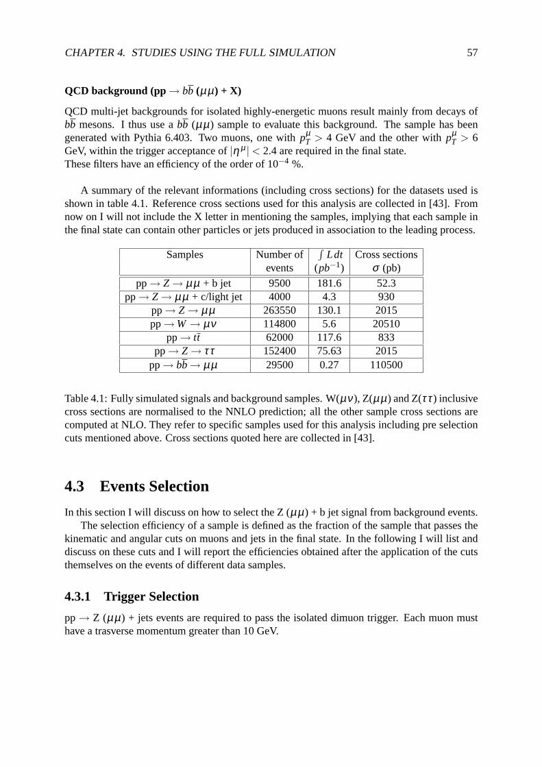
CHAPTER 4. STUDIES USING THE FULL SIMULATION 57
QCD background (pp→ bb (µµ) + X)
QCD multi-jet backgrounds for isolated highly-energetic muons result mainly from decays ofbb mesons. I thus use abb (µµ) sample to evaluate this background. The sample has beengenerated with Pythia 6.403. Two muons, one withpµ
T > 4 GeV and the other withpµT > 6
GeV, within the trigger acceptance of|η µ | < 2.4 are required in the final state.These filters have an efficiency of the order of 10−4 %.
A summary of the relevant informations (including cross sections) for the datasets used isshown in table 4.1. Reference cross sections used for this analysis are collected in [43]. Fromnow on I will not include the X letter in mentioning the samples, implying that each sample inthe final state can contain other particles or jets produced in association to the leading process.
Samples Number of∫
Ldt Cross sectionsevents (pb−1) σ (pb)
pp→ Z → µµ + b jet 9500 181.6 52.3pp→ Z → µµ + c/light jet 4000 4.3 930
pp→ Z → µµ 263550 130.1 2015pp→ W → µν 114800 5.6 20510
pp→ tt 62000 117.6 833pp→ Z → ττ 152400 75.63 2015
pp→ bb→ µµ 29500 0.27 110500
Table 4.1: Fully simulated signals and background samples.W(µν ), Z(µµ) and Z(ττ ) inclusivecross sections are normalised to the NNLO prediction; all the other sample cross sections arecomputed at NLO. They refer to specific samples used for this analysis including pre selectioncuts mentioned above. Cross sections quoted here are collected in [43].
4.3 Events Selection
In this section I will discuss on how to select the Z (µµ) + b jet signal from background events.The selection efficiency of a sample is defined as the fractionof the sample that passes the
kinematic and angular cuts on muons and jets in the final state. In the following I will list anddiscuss on these cuts and I will report the efficiencies obtained after the application of the cutsthemselves on the events of different data samples.
4.3.1 Trigger Selection
pp→ Z (µµ) + jets events are required to pass the isolated dimuon trigger. Each muon musthave a trasverse momentum greater than 10 GeV.

CHAPTER 4. STUDIES USING THE FULL SIMULATION 58
4.3.2 Muons
The muon reconstruction is done with the muon spectrometer combined with the inner detector(see also section 3.2.2 for further details).The Staco collection [35] is the current default for physicsanalysis inside the Atlas Collabo-ration but future analyses may make use of the Muid collection [34] or a mixture of muonsdrawn from both of these and any future collections. I used the Staco muon container requiringfor each event at least two muons with opposite charge. The reconstructed muon tracks shouldsatisfypT > 15 GeV and|η | < 2.4.Muons in jet tend to be produced within a decay cascade of further particles, and should there-fore not appear isolated in the detector, in contrast to the leptonic decays of Z boson. Isolation
is applied by requiring the angular distance between the twomuons (∆Rµµ =√
∆η 2µµ +∆φ2
µµ )
greater than 0.5.The invariant mass of the muon pair is required to fulfil 70 GeV< Mµµ < 110 GeV. If morethan two muons are reconstructed, the pair with the invariant mass closest to theMZ = 91.1876± 0.0021 [1] is chosen.
Figure 4.1 (a) shows the transverse momentum spectrum for all the muons found in theanalyzed data samples within|η | < 2.4, before any other cut is applied. Figure 4.1 (b) showsthe angular distance∆Rµµ between two muons of opposite charge, transverse momentum above15 GeV and|η | < 2.4. The two plots are scaled to
∫Ldt = 1fb−1 of integrated luminosity.
From figure 4.1 (b) it is clear that the decision to cut on the angular distance between the twomuons∆Rµµ > 0.5 has been taken primarly to reduce QCD (bb) background.
Pt (GeV)0 10 20 30 40 50 60 70 80 90 100
/ 4
Ge
V-1
Nu
mb
er o
f m
uo
ns
/ 1
fb
310
410
510
610
710
SamplesQCD (b bbar) t tbarZ tau tau Z inclusive Z + b jet Z + c/light jet W
ATLAS
Angular distance (DeltaR)0 0.5 1 1.5 2 2.5 3 3.5 4
/ 0
.2 D
R-1
Nu
mb
er
of
mu
on
s /
1 f
b
310
410
510
610
710 Samples
QCD (b bbar)
t tbar
Z tau tau
Z inclusive
Z + b jet
Z + c/light jet
W
ATLAS
(a) (b)
Figure 4.1: (a) : Distribution of the muon transverse momentum in |η | < 2.4 before any otherselection cut. (b): Distribution of the angular distance∆Rµµ between two muons of oppositecharge, transverse momentum above 15 GeV and|η |< 2.4. The two plots are scaled to
∫Ldt =
1fb−1 of integrated luminosity.

CHAPTER 4. STUDIES USING THE FULL SIMULATION 59
Figure 4.2 shows the invariant mass of the muon pair, after cuts on muons. The plot isnormalized to 1f b−1 integrated luminosity.
Μ µµ40 50 60 70 80 90 100 110 120
/ 2
Ge
V-1
Nu
mb
er
of
Ev
en
ts /
1 f
b
10
210
310
410
510
SamplesQCD (b bbar)
t tbarZ tau tau Z inclusive Z + b jet Z + c/light jet
W
ATLAS
Figure 4.2: Invariant mass of the muon pair after muon selection cuts. The plot is normalizedto 1 f b−1 integrated luminosity.
From this figure we see that cutting on muons considerably reduce backgrounds not con-taining a Z decaying into muons (tt , Z → ττ , W → µν and QCD multi-jetbb events). Thesubsequent request on the invariant mass range of the muon pair (70 GeV< Mµµ < 110 GeV)allows to an even better selection of the signal over the backgrounds of above.
4.3.3 Jets
In this thesis the standard cone algorithm jet reconstruction available in the ATLAS software isused. A jet is therefore defined by a direction, an energy and acone size that corresponds to thejet opening angle. I used jets clustered with the standard ATLAS seeded-cone algorithm with aradius of∆R=0.4, built from topological cluster (see section 3.2.2).It is required at least one jet in the event with transverse momentumpT > 20 GeV in the range|η | < 2.4. In order to remove jets faking muons in the signal analysis, the angular distancebetween Figure 4.3 shows the transverse momentum (a) and pseudo rapidity (b) distributionsfor signal and background events.
Figure 4.4 shows the transverse momentum (a) and pseudo rapidity (b) distributions of jetsafter cuts on muons and muon pair discussed in the previous section. All distribution are nor-malized to
∫Ldt = 1fb−1 of integrated luminosity.
.Comparing fig. 4.3 and fig. 4.4 we can conclude that the shape of distributions is not influ-
enced by the cuts on muons and muon pair. Those cuts only reduce the fraction of backgroundfrom the signal.

CHAPTER 4. STUDIES USING THE FULL SIMULATION 60
Pt (GeV)0 20 40 60 80 100 120 140 160 180 200
/ 4
Ge
V-1
Nu
mb
er
of
jets
/ 1
fb
210
310
410
510
610
710
SamplesQCD (b bbar) t tbarZ tau tau Z inclusive Z + b jet Z + c/light jet
W
ATLAS
Pseudo rapidity-5 -4 -3 -2 -1 0 1 2 3 4 5
/ 0.
2
-1N
um
ber
of
jets
/ 1
fb
310
410
510
610
710
SamplesQCD (b bbar) t tbarZ tau tau Z inclusive Z + b jet Z + c/light jet W
ATLAS
(a) (b)
Figure 4.3: Transverse momentum (a) and rapidity (b) distributions of jets.
Pt (GeV)0 20 40 60 80 100 120 140 160 180 200
/ 4
Ge
V-1
Nu
mb
er o
f je
ts /
1 f
b
10
210
310
410
510
610Samples
QCD (b bbar) t tbarZ tau tau Z inclusive Z + b jet Z + c/light jet W
ATLAS
Pseudo rapidity-5 -4 -3 -2 -1 0 1 2 3 4 5
/ 0.
2-1
Nu
mb
er o
f je
ts /
1 fb
10
210
310
410
510
SamplesQCD (b bbar) t tbarZ tau tau Z inclusive Z + b jet Z + c/light jet
W
ATLAS
(a) (b)
Figure 4.4: Transverse momentum (a) and rapidity (b) ditributions of jets after cuts on muonsinside the invariant mass range 70 GeV< Mµµ < 110 GeV and before any cut on jets.
4.3.4 Jet tagging
Realistic estimation of rejection/mistag rate is crucial tothe studies which depend on b-tagging.In this analysis jets are labelled as b-jets using the b tagging algorithm with the highest light-jetrejection power. This algorithm makes use of the 3D impact parameter and secondary-vertexreconstruction, IP3D+SV1. As already discussed in section3.2.2, tracks from B-hadrons de-cays are expected to have on average a large and positive transverse impact parametera0 and a

CHAPTER 4. STUDIES USING THE FULL SIMULATION 61
large and positive longitudinal impact parameterz0. Combining the longitudinal and trasversesignificance in the function:wt = Pb(Sa0,z0)/Pu(Sa0,z0) and applying a cut on the likehood func-tion is possible to discriminate b jets from c and light jets (see [45] for additional informationabout the algorithm).In this analysis I cut on the b tagging weight parameterweight≥ 5.An explanation on why the value of 5 has been chosen to cut on the b-tagging weight will begiven in the following section.
4.3.5 Tests of b-tagging
Here I will discuss how to choose the value for the b tagging weight parameter in order tomaximize both the efficiency in selecting Z + b jet events and the rejection of the backgroundswhere a Z is produced in association to a charm or a light jet and I will give an explanation onwhy it has been chosen to require the b tagging weight greaterthan 5.
Definitions and Events Selection
In order to define the Z + b jet efficiency and Z + c/light jet rejection, it is needed to know howmany jets derive from bottom, charm and light quarks. In other words, we need to know thetrue flavor of the jet from the Monte Carlo truth informations.I remind that a jet is labelled asa b-jet if a b quark withpT > 5 GeV is found in a cone size∆R=0.3 around the jet axis. Sameprocedure applies for c andτ jets. If no beauty or charm orτ is found, the jet is labelled as light(u, d, s, g).
In section 3.2.2 I definedb-jet efficiency, mistag probabilityand rejectionper jet, here Irecall the definitions and describe the cuts used in this analysis, but I will apply them per event.
TheZ + b jet efficiencyεb is defined as the ratio between the number of events containing atleast one Cone 0.4 true b-jet (from the MC truth informations)with ET > 15 GeV and|η |< 2.5above a chosen b tagging weight cut, and the number of events containing at least one Cone0.4 true b-jet inside the same transverse energy and rapidity ranges but before cutting on the btagging weight.
The Z + b jet mistag probabilityis the probability that a given event containing a non b-jet (from the MC truth informations) inside the same transverse energy and rapidity ranges(ET > 15 GeV and|η | < 2.5) is tagged ad a Z+ b-jet event (εmisc/l
).
TheZ + c/light jet rejectionfactor is defined as the inverse of, respectively, c and lightjetsmistag probability:Rc/l = 1/εmisc/l
. As an example R=100 means 1% mistag rate.
The b-tagging efficiency for Z + b jet events has been derived using the Monte Carlo samplepp → Z(µµ) + b jet , while the evaluation of the rejection factor for Z+c/light jet was doneusing the inclusive pp→ Z(µµ) sample (because of the poor statistic of pp→ Z(µµ) + c/lightjet sample).
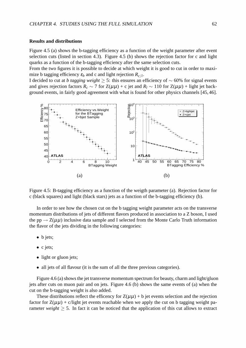
CHAPTER 4. STUDIES USING THE FULL SIMULATION 62
Results and distributions
Figure 4.5 (a) shows the b-tagging efficiency as a function ofthe weight parameter after eventselection cuts (listed in section 4.3). Figure 4.5 (b) showsthe rejection factor for c and lightquarks as a function of the b-tagging efficiency after the same selection cuts.From the two figures it is possible to decide at which weight itis good to cut in order to maxi-mize b tagging efficiencyεb and c and light rejectionRc/l .I decided to cut atb tagging weight≥ 5: this ensures an efficiency of∼ 60% for signal eventsand gives rejection factorsRc ∼ 7 for Z(µµ) + c jet andRl ∼ 110 for Z(µµ) + light jet back-ground events, in fairly good agreement with what is found for other physics channels [45,46].
BTagging Weight0 2 4 6 8 10
Effi
cien
cy %
40
45
50
55
60
65
70
75
80 Efficiency vs.Weightfor the BTaggingZ+bjet Sample
ATLAS
BTagging Efficiency %40 45 50 55 60 65 70 75 80
Rej
ectio
n
1
10
210
310
410
Z+lightjetZ+cjet
ATLAS
(a) (b)
Figure 4.5: B-tagging efficiency as a function of the weigth parameter (a). Rejection factor forc (black squares) and light (black stars) jets as a function of the b-tagging efficiency (b).
In order to see how the chosen cut on the b tagging weight parameter acts on the transversemomentum distributions of jets of different flavors produced in association to a Z boson, I usedthe pp→ Z(µµ) inclusive data sample and I selected from the Monte Carlo Truth informationthe flavor of the jets dividing in the following categories:
• b jets;
• c jets;
• light or gluon jets;
• all jets of all flavour (it is the sum of all the three previous categories).
Figure 4.6 (a) shows the jet transverse momentum spectrum for beauty, charm and light/gluonjets after cuts on muon pair and on jets. Figure 4.6 (b) shows the same events of (a) when thecut on the b-tagging weight is also added.
These distributions reflect the efficency for Z(µµ) + b jet events selection and the rejectionfactor for Z(µµ) + c/light jet events reachable when we apply the cut on b tagging weight pa-rameterweight≥ 5. In fact it can be noticed that the application of this cut allows to extract
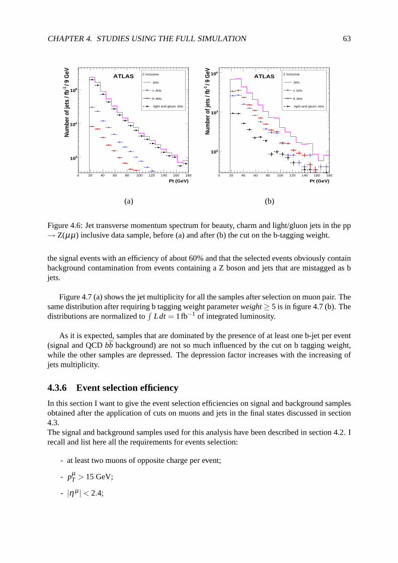
CHAPTER 4. STUDIES USING THE FULL SIMULATION 63
Pt (GeV)0 20 40 60 80 100 120 140 160 180
/ 9
GeV
-1N
umbe
r of j
ets
/ fb
310
410
510
Z inclusive
Jets
c Jets
b Jets
light and gluon Jets
ATLAS
Pt (GeV)0 20 40 60 80 100 120 140 160 180
/ 9
GeV
-1N
umbe
r of j
ets
/ fb
210
310
410 Z inclusive
Jets
c Jets
b Jets
light and gluon Jets
ATLAS
(a) (b)
Figure 4.6: Jet transverse momentum spectrum for beauty, charm and light/gluon jets in the pp→ Z(µµ) inclusive data sample, before (a) and after (b) the cut on the b-tagging weight.
the signal events with an efficiency of about 60% and that the selected events obviously containbackground contamination from events containing a Z boson and jets that are mistagged as bjets.
Figure 4.7 (a) shows the jet multiplicity for all the samplesafter selection on muon pair. Thesame distribution after requiring b tagging weight parameterweight≥ 5 is in figure 4.7 (b). Thedistributions are normalized to
∫Ldt = 1fb−1 of integrated luminosity.
As it is expected, samples that are dominated by the presenceof at least one b-jet per event(signal and QCDbb background) are not so much influenced by the cut on b tagging weight,while the other samples are depressed. The depression factor increases with the increasing ofjets multiplicity.
4.3.6 Event selection efficiency
In this section I want to give the event selection efficiencies on signal and background samplesobtained after the application of cuts on muons and jets in the final states discussed in section4.3.The signal and background samples used for this analysis have been described in section 4.2. Irecall and list here all the requirements for events selection:
- at least two muons of opposite charge per event;
- pµT > 15 GeV;
- |η µ | < 2.4;

CHAPTER 4. STUDIES USING THE FULL SIMULATION 64
Number of jets0 1 2 3 4 5
-1E
ve
nts
/ 1
fb
210
310
410
510
SamplesQCD (b bbar) t tbarZ tau tau Z inclusive Z + b jet Z + c/light jet W
ATLAS
Number of jets0 1 2 3 4 5
-1E
ven
ts /
1 fb
1
10
210
310
410
SamplesQCD (b bbar) t tbarZ tau tau Z inclusive Z + b jet Z + c/light jet W
ATLAS
(a) (b)
Figure 4.7: Jet multiplicity before cutting on jets (a) and after requiring b tag weight> 5 (b).All distributions have been obtained after cuts on muons andmuon pair invariant mass andnormalized to
∫Ldt = 1fb−1 of integrated luminosity.
- ∆Rµµ > 0.5;
- 70 GeV< Mµµ <110 GeV.
- ∆Rµ− jet > 0.4;
- p jetT > 15 GeV;
- |η jet| < 2.5;
The selection efficiency is defined as
ε =Nsel
Ntot(4.2)
whereNsel is the number of events selected after the requirements of above, whileNtot is thenumber of events in each original sample of Monte Carlo data (see table 4.1).The uncertainty on efficiency is of purely statistical origin.
The achievable efficiencies after the cuts on muons and muon pair invariant mass are shownin table 4.2. All cuts have been applied sequentially. The percentages are referred to the totalnumber of events in each sample.
After the selection of events that satisfies cuts on muons anddi-muon invariant mass, re-quirements on jets multiplicity, angular distance betweenjets and muons, transverse momen-tum, rapidity distribution and b tagging weight have been applyed. Efficiencies obtained apply-ing these cuts sequentially are listed in table 4.3.
Results of tables 4.2 and 4.3 have been used to estimate the fraction of signal and back-ground events in a selected sample of 1 fb−1 of data. These estimations allow to obtain the

CHAPTER 4. STUDIES USING THE FULL SIMULATION 65
Samples at least pµT > 15 GeV 70< Mµµ < 110
1 µ+ and 1µ− |η µ | < 2.4 GeV∆Rµ−µ > 0.5
Z → µµ 56.9±0.3 43.3±0.2 40.8±0.2Z → µµ + b jet 91.1±2.0 74.1±1.6 70.8±1.6
Z → µµ + c/light jet 92.7±3.0 74.1±2.5 69.4±2.4tt 11.4±0.1 1.8±0.1 0.49±0.03
W → µν 2.52±0.05 0.044±0.006 0.013±0.003Z → ττ 23.1±0.2 3.3±0.1 0.40±0.02QCDbb 76.1±0.1 0.12±0.02 0.06±0.01
Table 4.2: Selection efficiencies (expressed in %) after thecuts on muons and muon pair.
Samples at least 1 ∆Rµ− jet >0.4 p jetT > 20 GeV btag weight
jet per event |η jet| < 2.5 w jet > 5Z → µµ 28.8±0.2 22.0±0.1 14.9±0.1 1.13±0.02
Z → µµ + b jet 56.6±1.3 42.7±1.1 28.3±0.8 15.4±0.6Z → µµ + c/light jet 45.4±1.8 31.2±1.4 17.6±0.9 0.5±0.1
tt 0.49±0.03 0.39±0.03 0.39±0.03 0.34±0.02W → µν 0.013±0.003 0.010±0.003 0.010±0.003 0.009±0.001Z → ττ 0.29±0.01 0.23±0.01 0.15±0.01 0.020±0.003QCDbb 0.06±0.01 0.05±0.01 0.05±0.01 0.03±0.01
Table 4.3: Selection efficiencies (expressed in %) after thecuts on jets (cuts on muons fromtable 4.2 are also included).
number of background eventsB and the efficiency of the signal events (εS) that are in the for-mula 4.1. Such estimations will be discussed in the next section.
4.4 Number of events and ratio of cross sections
In this section I will give a first estimation of the expected number of events and the correspond-ing fraction of the total sample for signal and for the background channels after applying thecuts outlined in in section 4.3 for an integrated luminosityof 1fb−1.The obtained values will be used to evaluate the cross section ratio between the signalZ → µµ+ b jet and the inclusiveZ → µµ + jets cross section.
4.4.1 Number of events
The number of eventsNev passing a given set of selections is expressed as follows:
Nev = L σ ε (4.3)
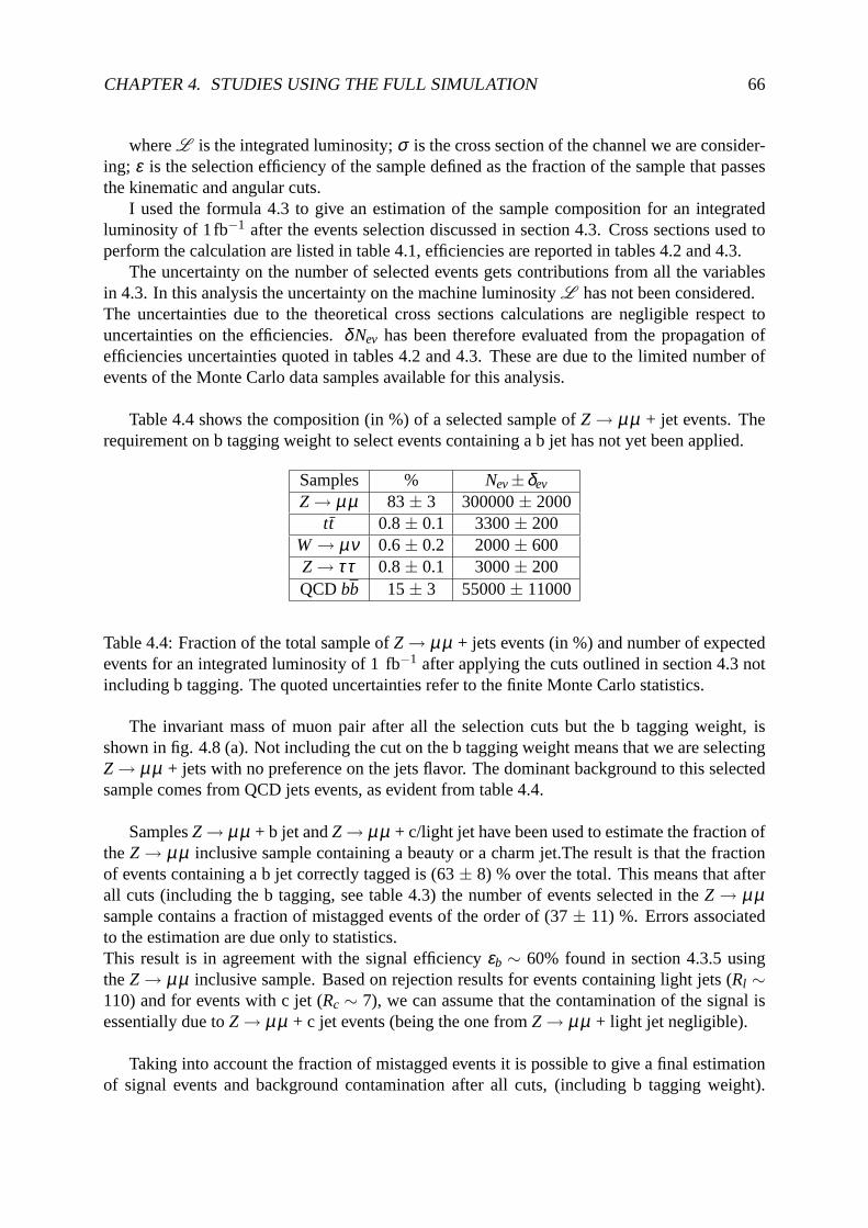
CHAPTER 4. STUDIES USING THE FULL SIMULATION 66
whereL is the integrated luminosity;σ is the cross section of the channel we are consider-ing; ε is the selection efficiency of the sample defined as the fraction of the sample that passesthe kinematic and angular cuts.
I used the formula 4.3 to give an estimation of the sample composition for an integratedluminosity of 1fb−1 after the events selection discussed in section 4.3. Cross sections used toperform the calculation are listed in table 4.1, efficiencies are reported in tables 4.2 and 4.3.
The uncertainty on the number of selected events gets contributions from all the variablesin 4.3. In this analysis the uncertainty on the machine luminosityL has not been considered.The uncertainties due to the theoretical cross sections calculations are negligible respect touncertainties on the efficiencies.δNev has been therefore evaluated from the propagation ofefficiencies uncertainties quoted in tables 4.2 and 4.3. These are due to the limited number ofevents of the Monte Carlo data samples available for this analysis.
Table 4.4 shows the composition (in %) of a selected sample ofZ → µµ + jet events. Therequirement on b tagging weight to select events containinga b jet has not yet been applied.
Samples % Nev±δev
Z → µµ 83± 3 300000± 2000tt 0.8± 0.1 3300± 200
W → µν 0.6± 0.2 2000± 600Z → ττ 0.8± 0.1 3000± 200QCDbb 15± 3 55000± 11000
Table 4.4: Fraction of the total sample ofZ → µµ + jets events (in %) and number of expectedevents for an integrated luminosity of 1 fb−1 after applying the cuts outlined in section 4.3 notincluding b tagging. The quoted uncertainties refer to the finite Monte Carlo statistics.
The invariant mass of muon pair after all the selection cuts but the b tagging weight, isshown in fig. 4.8 (a). Not including the cut on the b tagging weight means that we are selectingZ → µµ + jets with no preference on the jets flavor. The dominant background to this selectedsample comes from QCD jets events, as evident from table 4.4.
SamplesZ → µµ + b jet andZ → µµ + c/light jet have been used to estimate the fraction oftheZ → µµ inclusive sample containing a beauty or a charm jet.The result is that the fractionof events containing a b jet correctly tagged is (63± 8) % over the total. This means that afterall cuts (including the b tagging, see table 4.3) the number of events selected in theZ → µµsample contains a fraction of mistagged events of the order of (37 ± 11) %. Errors associatedto the estimation are due only to statistics.This result is in agreement with the signal efficiencyεb ∼ 60% found in section 4.3.5 usingtheZ → µµ inclusive sample. Based on rejection results for events containing light jets (Rl ∼110) and for events with c jet (Rc ∼ 7), we can assume that the contamination of the signal isessentially due toZ → µµ + c jet events (being the one fromZ → µµ + light jet negligible).
Taking into account the fraction of mistagged events it is possible to give a final estimationof signal events and background contamination after all cuts, (including b tagging weight).
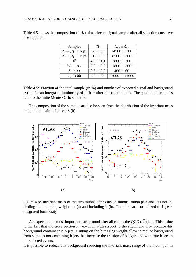
CHAPTER 4. STUDIES USING THE FULL SIMULATION 67
Table 4.5 shows the composition (in %) of a selected signal sample after all selection cuts havebeen applied.
Samples % Nev±δev
Z → µµ + b jet 25± 5 14500± 200Z → µµ + c jet 13± 3 8500± 200
tt 4.5± 1.1 2800± 200W → µν 2.9± 0.8 1800± 200Z → ττ 0.6± 0.2 400± 60QCDbb 63± 34 33000± 11000
Table 4.5: Fraction of the total sample (in %) and number of expected signal and backgroundevents for an integrated luminosity of 1 fb−1 after all selection cuts. The quoted uncertaintiesrefer to the finite Monte-Carlo statistics.
The composition of the sample can also be seen from the distribution of the invariant massof the muon pair in figure 4.8 (b).
µ µΜ70 75 80 85 90 95 100 105 110
/ 2
Ge
V-1
Nu
mb
er
of
Ev
en
ts /
1 f
b
10
210
310
410
SamplesQCD (b bbar)
t tbarZ tau tau Z inclusive Z + b jet Z + c/light jet
W
ATLAS
µ µΜ70 75 80 85 90 95 100 105 110
/ 2
GeV
-1N
um
ber
of
Even
ts / 1
fb
10
210
310
SamplesQCD (b bbar) t tbarZ tau tau Z inclusive Z + b jet Z + c/light jet W ATLAS
(a) (b)
Figure 4.8: Invariant mass of the two muons after cuts on muons, muon pair and jets not in-cluding the b tagging weight cut (a) and including it (b). Theplots are normalized to 1f b−1
integrated luminosity.
As expected, the most important background after all cuts isthe QCD (bb) jets. This is dueto the fact that the cross section is very high with respect tothe signal and also because thisbackground contains true b jets. Cutting on the b tagging weight allow to reduce backgroundfrom samples not containing b jets, but increase the fraction of background with true b jets inthe selected events.It is possible to reduce this background reducing the invariant mass range of the muon pair in

CHAPTER 4. STUDIES USING THE FULL SIMULATION 68
order to exclude a bigger fraction of (bb) events. If I cut on the invariant mass rangeMZ± 10GeV (instead of the previous 70< Mµµ < 110 GeV) leaving unchanged all other cuts on muonsand jets, the fraction of the signal sample increases respect to the background.
Results after applying all cuts on muons and jets in the new invariant mass range ofMZ±10 GeV are shown in table 4.6. Errors are due only to statistics.
Samples % Nev±δev
Z → µµ + b jet 45± 9 13600± 200Z → µµ + c jet 24± 5 7200± 200
tt 5.1± 1.5 1600± 200W → µν 0.6± 0.6 200± 200Z → ττ 0.3± 0.2 100± 40QCDbb 25± 22 7700± 5500
Table 4.6: Fraction of the total sample (in %) and number of expected signal and backgroundevents for an integrated luminosity of 1 fb−1 after all selection cuts in the invariant mass rangeof Mµµ± 10 GeV. The quoted uncertainties refer to the finite Monte-Carlo statistics.
In this case the QCD (bb) has been reduced and we can also see that the error associated tothis background estimation is very big due to the limited statistics of the sample itself. More wereduce the mass range and more the low statistic does not allow to have a precise estimation ofthis background.In order to better estimate the contamination of the signal due to this background further studiesare required with larger QCD jets MC samples. Neverthless, inthe future it will be possible toreduce the percentage from this backgrond exploiting different methods. One of this methodcould be to fit on the di-muon pair invariant mass.
In addition, Tevatron experience [47, 48] make us confident that real data will help in im-proving the discrimination between signal and QCD (bb) jets background. In such a case one ofthe main background remains Z(µµ) + c jet . A method to better discriminate this backgroundfrom the signal will be discussed in the next chapter.
4.4.2 Ratio of cross sections
In this section I want to give a first estimation of cross section ratio between the signalZ → µµ+ b jet and the inclusiveZ → µµ + jets cross section using results reported in tables 4.4 and4.5. Looking at ratios instead of a single cross section is also useful because some systematicuncertainties can be partially removed.
The value obtained from the analysis described in the previous section is the following:
[σ(Z → µµ +b jet)σ(Z → µµ + jets)
]analysis= 0.048±0.001 (4.4)
The uncertainty refers only to the finite Monte Carlo statistics.

CHAPTER 4. STUDIES USING THE FULL SIMULATION 69
We can make a comparison between this result and the theoretical prediction obtained run-ning the MCFM [29] program within the same cuts on muons, muon pair and jets that havebeen used in the analysis to select the signal (see sec. 4.3).The cone algorithm 0.4 has beenchosen to define jets and the PDF sets CTEQ6M has been used.
The cross section obtained with MCFM for the signal channel isin agreement with the onefound from the analysis on Monte Carlo data samples:
[σ(Z → µµ +b jet)σ(Z → µµ + jets)
]MCFM = 0.0479±0.0002 (4.5)
Theoretical uncertainties have been automatically estimated by MCFM. They arise from thechoice of the renormalisation and factorisation scales, and they also include PDF uncertainty.
The same ratio has been already evaluated by CDF [48] and D0 [49] experiments at Teva-tron, finding a very good agreement with theoretical predictions calculated using the MCFMprogram.
4.5 b-tagging algorithm using pp→ W (µν) inclusive sample
For analysis using b tagging, the estimation of the backgrounds from well-known StandardModel processes requires to know the tagging and mistaggingefficiency for the various fla-vors of jets with high accuracy. The quality of Monte Carlo simulation of these properties isunknown and therefore strategies must be developed to measure the tagging and mistagging ef-ficiencies directly from data. The b-tagging efficiency can be checked usingb-enriched samples.
We have seen in the previous section that a non negligible amount of background in theselected sample is due to mis-tagged jets from c and light quarks. This can be controlled bylooking at the number of tagged jets in data samples that in principle should not containb-jetsat first order:W + jets production, for example, is such a kind of events.TheW + jets events will be available with large statistics, in addition jets produced in associa-tion with W boson will cover the fullpT range of the signal.
The inclusiveW → µν sample has been used to estimate the mis tagging rate as a functionof the transverse momentum of the jet produced in association to the W boson.
4.5.1 Events Selection and Results
I analized events containing a muon fromW decay within kinematic cuts on muon and jets inthe final state already listed in section 4.3. I recall them here:
• at least one muon in the event with:
- pµT > 15 GeV;
- |η µ | < 2.4;
• at least one reconstructed Cone 0.4 jet with:.

CHAPTER 4. STUDIES USING THE FULL SIMULATION 70
- p jetT > 20 GeV;
- |η jet| < 2.5;
After these selections, I looked for events where at least one jet is tagged as ab-jet by theb-tagging algorithm (w jet > 5). In this way it has been possible to calculate the number ofeventwith at least one mistagged jet with respect to the total number of events as function of the jettransverse momentumpT .As we can see in figure 4.9 we expect a mistagging rate at the level of few percent over the fullpT range of the signal per event.This result is in good agreement with previous results obtained using fast simulation on aW+jetsample [63].
Pt (GeV)20 30 40 50 60 70 80 90 100
mis
-tag
rat
e
0.01
0.02
0.03
0.04
0.05
0.06
0.07
0.08
0.09
0.1ATLAS (Full Simulation)
Figure 4.9: Mistagging rate ofb-jets evaluated from fraction of b-tagging jets in the pp→ W(µν) sample: relative error on background level per 5 GeV jetpT bin.

Chapter 5
Studies using the FAST simulation
The production of data sample used to perform the analysis discussed in this chapter has beendone inside the Athena framework. The Monte Carlo chosen to produce these data samples isPYTHIA.The pseudo data obtained with the fast simulation have been used basically for two reasons: toperform preliminary studies on the parton distribution function of the b quark using differentPDF sets and to study the behaviour of some variables that canhelp in distinguishing b jetsfrom c jets. This latter study was done to see if is it possibleto find variables that allow to reacha better or comparable efficiency and purity of the signal andin particular a better rejection ofZ(µµ) + c jet events respect to the one obtained using the b taggingweight variable.
5.1 Preliminary studies ofb density function
An important source of theoretical systematic uncertainties at the LHC is represented by theParton Distribution Functions (PDF). If the understandingof the perturbative corrections tothe hard scattering in theZ inclusive andZ+ jets cross sections is in good shape [62], the un-certainty on the PDFs can limit the accuracy of the theoretical predictions on cross sectionmeasurements. This uncertainty will limit the differential cross section measurements and dis-tributions of various observables in different channels (for example the transverse momentum,the rapidity distribution of weak bosons or jets).
In this section I will show a preliminary study involving twodifferent PDF sets in the pp→ Z(µµ) + jets channel: CTEQ6l [50] and MRST2004 [52]. The study has thepurpose togive a first rough estimation of the impact of the PDF uncertainty on transverse momentum andrapidity distribution of theZ boson produced in association to a b-jet.
5.1.1 Monte Carlo Data Samples
The samples used for this study have been generated with the PYTHIA Monte Carlo package[24] interfaced to the library containing informations about different PDF sets: LHAPDF [58].The detector response has been simulated using the ATLFAST package [39].
71

CHAPTER 5. STUDIES USING THE FAST SIMULATION 72
In order to produce these samples I started from the official JobOption used by the Atlas col-laboration to generate and fully simulate the pp→ Z(µµ) inclusive channel [57]. The aboveJobOption has been modified to require the presence of at least one jet in the final state, tochange the PDF sets and to be interfaced to the ATLFAST package.
The following samples have been produced:
• pp→ Z(µµ) + jets : CTEQ6l [50];
• pp→ Z(µµ) + jets : MRST2004 [52].
The two samples have been generated without requiring any filter on muons from the Zdecay, but asking for a transverse momentum of the the jets greater than 10 GeV in order toavoid divegences in the cross sections. 200K events have been generated for each of the abovesamples. The energy scale and Bjorken variable range of validity for each PDF sets is reportedin table 5.1 . For the study discussed in this thesis, the two ranges are equivalent, since we arenot sensible tox values less than 10−5 GeV2 andQ2 bigger than 107 GeV2.
PDF set xmin xmax Q2min Q2
max(GeV2) (GeV2)
CTEQ6l 10−6 1 1.69 108
MRST2004 10−5 1 1.25 107
Table 5.1: Energy scale and Bjorken variable range of validity for each set of PDF .
5.1.2 b parton and b jets distributions
In this section I want to discuss if the discrepancies between transverse momentum or rapid-ity distributions of the b jets obtained with different PDF sets are due to the hadronization andreconstruction procedure or to the intrinsic differences in the treatment of b parton density func-tion between CTEQ and MRST collaborations. In the latter case we could use this differenceto estimate the uncertainty on differential cross section measurements for the Z (µµ) + b jetchannel due to the b PDF. For this purpose I will show a comparison between distributions oftrue b quarks (identified from the Monte Carlo Truth) and reconstructed b-jets (tagged from theATLFAST b tagging algorithm discussed in section 3.3.1).
In order to select theZ+b-jet signal I applied cuts both at parton level (on Monte Carlo Truthb partons) and at reconstruction level (on ATLFAST b-jets).I required al least one b parton/jetper event with transverse momentumpT > 15 GeV, and inside the pseudorapity range|η |< 2.5.Motivations for these choice have been already discussed insection 5.2.1.
Figure 5.1 assures that detector effects do not modify the shape ofpT and rapidity distribu-tion of the b jet. They have been obtained using the CTEQ6l PDF set, but same results can beobtained using MRST2004. All the plots are normalized to the number of entries.

CHAPTER 5. STUDIES USING THE FAST SIMULATION 73
Rapidity-5 -4 -3 -2 -1 0 1 2 3 4 5
No
rma
lize
d e
ve
nts
/ 0
.5 r
ap
idit
y
0
0.02
0.04
0.06
0.08
0.1
0.12 CTEQ6l
ATLFAST
MCTRUTH
Rapidity of b
Pt (GeV)0 10 20 30 40 50 60 70 80 90 100
no
rmal
ized
eve
nts
/ 1
GeV
0
0.01
0.02
0.03
0.04
0.05
0.06 CTEQ6l
ATLFAST
MC TRUTH
Transverse momentum of b
(a) (b)
Figure 5.1: Comparison between MC TRUTH and ATLFAST reconstruction of b distributionsin Z+b events:η (a) andpT (b) distributions of the b parton (MC TRUTH: dotted line) andjet(ATLFAST) .
Rapidity-5 -4 -3 -2 -1 0 1 2 3 4 5
/ 0
.5-1
Nu
mb
er
of
b j
ets
/ 1
fb
500
1000
1500
2000
2500 ATLFAST
CTEQ6lMRST2004
Rapidity of b-jet
pt (GeV)0 10 20 30 40 50 60 70 80 90 100
/ 2
GeV
-1N
um
ber
of
b je
ts /
1 fb
0
200
400
600
800
1000
1200
1400
1600
1800
ATLFAST
CTEQ6l
MRST2004
Transverse momentum of b jet
(a) (b)
Figure 5.2: (a)η distribution of the b-jets in Zb events (ATLFAST) (b)pT distribution of theb-jets in Zb events (ATLFAST).

CHAPTER 5. STUDIES USING THE FAST SIMULATION 74
The difference in transverse momentum and rapidity distributions of the b-jet using the twoPDF sets is shown in fig. 5.2. The plots are normalized to 1f b−1 of integrated luminosity.Only in the central rapity and low transverse momentum distributions we have differences of≈ 5% between the two sets of PDF. Neverthless comparing these distributions with fig. 5.1 wecan conclude that the only discrepancy that can be used to estimate the uncertainty on differ-ential cross section measurements for the Z+b jet channel due to the b PDF is the one in thecentral rapidity region: this discrepancy is absent when wecompare Monte Carlo true b quarkswith ATLFAST reconstructed b-jets. This should mean that the discrepancy is not due to thehadronization or to the reconstruction procedure, but to a difference between the two PDF sets.The same does not happen in the transverse momentum distributions: when we compare theMonte Carlo true b quarks and the ATLFAST reconstructed b-jets momentum distribution wesee that it already presents a discrepancy in the lowpT region.Anyway further studies including errors associated to the PDF should be done in order to givea more precise estimation of this discrepancy.
5.2 Studies of background from Z+c-jet
The measurement of theZ + b-jet cross section will be limited by systematic uncertainties andone important source of systematic uncertainty is related to the background due to c-jets thatare misidentified as b-jets.The identification ofb-jets takes advantage of several of their properties which allow us to dis-tinguish them from jets which contain only lighter quarks. First of all being the fragmentationhard, theb-hadron retains about 70% of the originalb quark momentum. Furthermore, the massof b-hadrons is relatively high (> 5 GeV), thus, their decay products have the opening angleof the decay products large enough to allow separation and a large transverse momentum withrespect to the jet axis. The third property is the relativelylong lifetime of hadrons containing ab quark, of the order of 1.5 ps (cτ ≈ 450µm). I remind here (see also sec. 3.2.2) that ab-hadronin a jet with pT = 10 GeV will therefore have a significant flight path length〈l〉 = βγcτ , trav-eling on average about 1 mm before decaying. Such displaced vertices can first be identifiedinclusively by measuring the impact parameters of the tracks from theb-hadron decay products.As already mentioned in section 3.3.1, I remind that the transverse impact parameter,d0, is thedistance of closest approach of the track to the primary vertex point, in ther −ϕ plane. Thelongitudinal impact parameter,z0, is thezcoordinate of the track at the point of closest approachin the beam line direction. The tracks fromb-hadron decay products tend to have rather largeimpact parameters which can be distinguished from tracks stemming from the primary vertex.This approach will be referred to later on asimpact parameter b-tagging.Finally, the semi-leptonic decays ofb-hadrons can be used by tagging the lepton in the jet. Inaddition, thanks to the hard fragmentation and high mass ofb-hadrons, the lepton will have alarge momentum relative to the jet axis. This is the so-called soft lepton tagging(the leptonbeing soft compared to high-pT leptons from Z decays).
In this section I will discuss the behaviour of some variables that could be used to distinguishZ+b-jet fromZ+c-jet events, with the goal of being able to measure both type of events. I amalso going to show that, rather than cutting on the single variables, an alternative approachfor the precise estimation of such background could be a Multivariate Analysis where selected

CHAPTER 5. STUDIES USING THE FAST SIMULATION 75
variables are taken into account simultaneously by a complex algorithm (i.e. Neural Network,Likelihood Estimator, etc) to discriminate between signaland background. The description ofthese algorithms can be found in [55].This study is motivated by the idea to find variables different from the ones used so far toconstruct the b tagging weight and to see if they can be combined in such a way to increase thepurity of Z+b-jet sample, reducing the background from mistaggedZ+c-jet events.
5.2.1 Simulated Data Sample and Event selection
All the samples have been generated with the PYTHIA Monte Carlo package [24]. The detectorresponse has been simulated using the ATLFAST package [39].In order to produce these samples I started from the official JobOption used by the Atlas col-laboration to generate and fully simulate the pp→ Z(µµ) inclusive channel [57]. The aboveJobOption has been modified to require the presence of at least one jet of a precise flavor asso-ciated to theZ boson in the final state and in order to be interfaced to the ATLFAST package.The contribution from virtual photon production (Drell-Yan) was switched off.
The following samples have been produced:
• pp→ Z → µµ + b jet + X;
• pp→ Z → µµ + c jet + X.
From now on I will not include the X letter in mentioning the samples, implying that eachsample in the final state can contains other particles and jets produced in association to the lead-ing process.The above samples have been produced in two ways: first with only the hard process and sub-sequent fragmentation and conversion of partons into hadrons that can decay if they are notstable (but any initial or final state radiation (ISR, FSR) and underlying event (UE)) and secondincluding also ISR, FSR and UE (for more details see sec. 3.1.1). For simplicity from now on Iwill refere to the first kind of samples asonly hard processsamples implying that hadronizationand decay of unstable particles are always included. Pile upinteractions coming from superpo-sition of different events are not present in the produced samples.The number of generated events, Pythia cross sections per samples and the corresponding inte-grated luminosity are reported in Table 5.2.
Only hard process Hard process + ISR, FSR, UEProcess Events Pythia
∫Ldt Pythia
∫Ldt
Cross Section (pb) (pb−1) Cross Section (pb) (pb−1)Z + b-jet 50K 40.03 1250 40.47 1235Z + c-jet 50K 49.48 1010 49.41 1010
Table 5.2: Number of generated events, Pythia cross sections and integrated luminosity forgenerated samples.

CHAPTER 5. STUDIES USING THE FAST SIMULATION 76
The analysis has been perfomed using the informations stored into the ntuples, in particularthe muons, the jets and the tracks blocks already defined in section 3.3.1.The Cone 0.4 jet algorithm has been used for the jet reconstruction.As it has been shown in the previous chapter cuts on muons and muon pair do not influence thedistributions of jets, so in order not to loose statistic, I decided to cut only on jets. I requiredat least one jet in the event with transverse momentump jet
T > 15 GeV and inside the rapidityrange|η jet| < 2.5.
In table 5.3 the number of events obtained after applying theselection cuts on the generatedsamples with only hard process is shown.
MC TRUTH (HARD PROCESS ONLY) ATLFAST (HARD PROCESS ONLY)Cuts Z+ b-jet Z+c-jet Cuts Z+b-jet Z+c-jet
Events Events Events Eventsat least 1 MC jet 43542 48332 at least 1 reco jet 31793 38388p jet
T > 15 GeV 28488 32146 p jetT > 15 GeV 24586 29689
|η jet| < 2.5 23740 26953 |η jet| < 2.5 20297 24565
Table 5.3: Number of events after cuts (only hard process).
In table 5.4 the number of events obtained after the selection cuts on the generated samplewith also ISR, FSR and UE switched on is shown.
MC TRUTH (FULL PROCESS) ATLFAST (FULL PROCESS)Cuts Z + b jet Z + c jet Cuts Z + b jet Z + c jet
Events Events Events Eventsat least 1 MC jet 47858 49527 at least 1 reco jet 37895 43961p jet
T > 15 GeV 34160 39569 p jetT > 15 GeV 28647 35368
|η jet| < 2.5 30080 35408 |η jet| < 2.5 24598 30963
Table 5.4: Number of events after cuts (ISR, FSR and UE switched on).
For the selected events the following variables have been studied:
• invariant mass of charged tracks in the jet;
• maximum impact parameter among the charged tracks in the jet;
• relative transverse momentum between the jet axis and the candidate muon from b or cdecay.
In section 5.2.2 the results obtained using only the first twoof these variables will be dis-cussed. In section 5.2.3 also the relative transverse momentum will be added to perform theanalysis.

CHAPTER 5. STUDIES USING THE FAST SIMULATION 77
Multivariate Analysis
In the following sections the preliminary results obtainedanalyzing the variables describedabove with the Toolkit for Multivariate Analysis (TMVA) [55] will be shown.The analysis proceeds by first choosing variables that can help in distinguishing signal frombackground events. For each variable, statistical properties like mean, variable ranges are com-puted to search for optimal cuts. Cut optimisation requires an estimator that quantifies thegoodness of a given cut ensemble. TMVA provides a ROOT [56] integrated environment forthe evaluation of multivariate classification techniques (classifiers) and the user can choose be-tween a whole set of such classifiers. Maximising this estimator minimises (maximises) thebackground efficiency,εB (background rejection,rB = 1− εB) for each signal efficiencyεS.The main advantage in using a Multivariate Analysis is essentially because it does not applycuts on variables in sequence, but it makes a combination of chosen variables in order not toreduce the initial sample (like we do when we cut sequentially) and to enhance efficiency onsignal selection and backgroud rejection. TMVA is widely used in High Energy Physics.For this first exercise I have used the following three classifiers: Fisher Discriminant, MultiLayer Perceptron (MLP) Neural Network and Likelihood Estimator.
The Likelihood Estimator consists of building a model of probability density functions thatreproduces the input variables for signal and background. For a given event, the likelihood forbeing of signal type is obtained by multiplying the signal probability densities of all input vari-ables, and normalising this by the sum of the signal and background likelihoods. Correlationsamong the variables are ignored.The Fisher Discriminant event selection is performed in a transformed variable space with zerolinear correlations, by distinguishing the mean values of the signal and background distribu-tions. No discrimination at all is achieved when a variable has the same sample mean for signaland background, even if the shapes of the distributions are very different.The Multi Layer Perceptron organizes the neurons in layers and only allowing directional con-nections from one layer to the immediate next one. Each directional connection between theoutput of one neuron and the input of another has an associated weight. The value of the outputneuron is multiplied with the weight to be used as input valuefor the next neuron.
A typical TMVA analysis consists of two indipendent phases:
- the training phase, where the multivariate classifiers aretrained, tested and evaluated,using two separate input data files: one for the signal and onefor the background;
- the application phase, where the trained classifiers are applied to the classification prob-lem implemented by the user in the analysis, using a more realistic input data file with amixture of signal and background events.
So far only the training phase has been implemented in this analysis. Work is in progress toimplement also the application phase.
The Multivariate Analysis has been performed on the sampleswith ISR, FSR and UEswitched off, in order to have a better control on the variables.
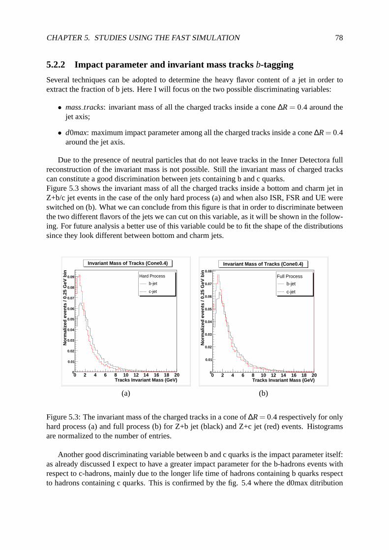
CHAPTER 5. STUDIES USING THE FAST SIMULATION 78
5.2.2 Impact parameter and invariant mass tracksb-tagging
Several techniques can be adopted to determine the heavy flavor content of a jet in order toextract the fraction of b jets. Here I will focus on the two possible discriminating variables:
• masstracks: invariant mass of all the charged tracks inside a cone∆R= 0.4 around thejet axis;
• d0max: maximum impact parameter among all the charged tracks inside a cone∆R= 0.4around the jet axis.
Due to the presence of neutral particles that do not leave tracks in the Inner Detectora fullreconstruction of the invariant mass is not possible. Stillthe invariant mass of charged trackscan constitute a good discrimination between jets containing b and c quarks.Figure 5.3 shows the invariant mass of all the charged tracksinside a bottom and charm jet inZ+b/c jet events in the case of the only hard process (a) and when also ISR, FSR and UE wereswitched on (b). What we can conclude from this figure is that inorder to discriminate betweenthe two different flavors of the jets we can cut on this variable, as it will be shown in the follow-ing. For future analysis a better use of this variable could be to fit the shape of the distributionssince they look different between bottom and charm jets.
Tracks Invariant Mass (GeV)0 2 4 6 8 10 12 14 16 18 20
No
rmal
ized
eve
nts
/ 0.
25 G
eV b
in
0
0.01
0.02
0.03
0.04
0.05
0.06
0.07
0.08
0.09 Hard Process
b-jet
c-jet
Invariant Mass of Tracks (Cone0.4)
Tracks Invariant Mass (GeV)0 2 4 6 8 10 12 14 16 18 20
No
rmal
ized
eve
nts
/ 0.
25 G
eV b
in
0
0.01
0.02
0.03
0.04
0.05
0.06
0.07
0.08
Full Process
b-jet
c-jet
Invariant Mass of Tracks (Cone0.4)
(a) (b)
Figure 5.3: The invariant mass of the charged tracks in a coneof ∆R= 0.4 respectively for onlyhard process (a) and full process (b) for Z+b jet (black) and Z+c jet (red) events. Histogramsare normalized to the number of entries.
Another good discriminating variable between b and c quarksis the impact parameter itself:as already discussed I expect to have a greater impact parameter for the b-hadrons events withrespect to c-hadrons, mainly due to the longer life time of hadrons containing b quarks respectto hadrons containing c quarks. This is confirmed by the fig. 5.4 where the d0max ditribution
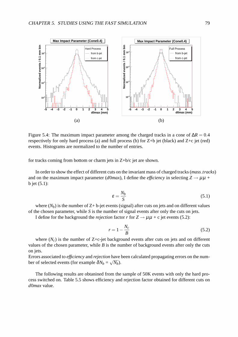
CHAPTER 5. STUDIES USING THE FAST SIMULATION 79
d0max (mm)-5 -4 -3 -2 -1 0 1 2 3 4 5
No
rmal
ized
eve
nts
/ 0.
1 m
m b
in
-410
-310
-210
-110
Hard Process
from b-jet
from c-jet
Max Impact Parameter (Cone0.4)
d0max (mm)-5 -4 -3 -2 -1 0 1 2 3 4 5
No
rmal
ized
eve
nts
/ 0.
1 m
m b
in
-410
-310
-210
-110
Full Process
from b-jet
from c-jet
Max Impact Parameter (Cone0.4)
(a) (b)
Figure 5.4: The maximum impact parameter among the charged tracks in a cone of∆R= 0.4respectively for only hard process (a) and full process (b) for Z+b jet (black) and Z+c jet (red)events. Histograms are normalized to the number of entries.
for tracks coming from bottom or charm jets in Z+b/c jet are shown.
In order to show the effect of different cuts on the invariantmass of charged tracks (masstracks)and on the maximum impact parameter (d0max), I define theefficiencyin selectingZ → µµ +b jet (5.1):
ε =Nb
S(5.1)
where (Nb) is the number of Z+ b-jet events (signal) after cuts on jets and on different valuesof the chosen parameter, whileS is the number of signal events after only the cuts on jets.
I define for the background therejectionfactorr for Z → µµ + c jet events (5.2):
r = 1− Nc
B(5.2)
where (Nc) is the number of Z+c-jet background events after cuts on jets and on differentvalues of the chosen parameter, whileB is the number of background events after only the cutson jets.Errors associated toefficiencyandrejectionhave been calculated propagating errors on the num-ber of selected events (for exampleδNb =
√Nb).
The following results are obtanined from the sample of 50K events with only the hard pro-cess switched on. Table 5.5 shows efficiency and rejection factor obtained for different cuts ond0maxvalue.
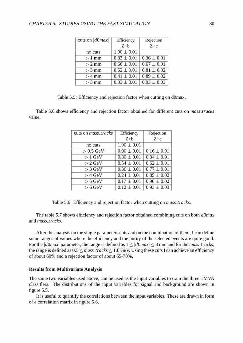
CHAPTER 5. STUDIES USING THE FAST SIMULATION 80
cuts on|d0max| Efficiency RejectionZ+b Z+c
no cuts 1.00± 0.01> 1 mm 0.83± 0.01 0.36± 0.01> 2 mm 0.66± 0.01 0.67± 0.01> 3 mm 0.52± 0.01 0.81± 0.02> 4 mm 0.41± 0.01 0.89± 0.02> 5 mm 0.33± 0.01 0.93± 0.03
Table 5.5: Efficiency and rejection factor when cutting on d0max.
Table 5.6 shows efficiency and rejection factor obtained fordifferent cuts onmasstracksvalue.
cuts onmasstracks Efficiency RejectionZ+b Z+c
no cuts 1.00± 0.01> 0.5 GeV 0.90± 0.01 0.16± 0.01> 1 GeV 0.80± 0.01 0.34± 0.01> 2 GeV 0.54± 0.01 0.62± 0.01> 3 GeV 0.36± 0.01 0.77± 0.01> 4 GeV 0.24± 0.01 0.85± 0.02> 5 GeV 0.17± 0.01 0.90± 0.02> 6 GeV 0.12± 0.01 0.93± 0.03
Table 5.6: Efficiency and rejection factor when cutting onmasstracks.
The table 5.7 shows efficiency and rejection factor obtainedcombining cuts on bothd0maxandmasstracks.
After the analysis on the single parameters cuts and on the combination of them, I can definesome ranges of values where the efficiency and the purity of the selected events are quite good.For the|d0max| parameter, the range is defined as 1≤ |d0max| ≤ 3 mm and for themasstracks,the range is defined as 0.5≤masstracks≤ 1.0 GeV. Using these cuts I can achieve an efficiencyof about 60% and a rejection factor of about 65-70%.
Results from Multivariate Analysis
The same two variables used above, can be used as the input variables to train the three TMVAclassifiers. The distributions of the input variables for signal and background are shown infigure 5.5.
It is useful to quantify the correlations between the input variables. These are drawn in formof a correlation matrix in figure 5.6.

CHAPTER 5. STUDIES USING THE FAST SIMULATION 81
cuts on 2 variables Efficiency RejectionZ+b Z+c
masstracks> 0.5 GeV& 0.78± 0.01 0.43± 0.01
|d0max| > 1 mmmasstracks> 0.5 GeV
& 0.63± 0.01 0.69± 0.01|d0max| > 2 mm
masstracks> 0.5 GeV& 0.50± 0.01 0.83± 0.02
|d0max| > 3 mmmasstracks> 1 GeV
& 0.70± 0.01 0.53± 0.01|d0max| > 1 mm
masstracks> 1 GeV& 0.57± 0.01 0.75± 0.01
|d0max| > 2 mmmasstracks> 1 GeV
& 0.45± 0.01 0.86± 0.02|d0max| > 3 mm
Table 5.7: Efficiency and rejection factor when cutting bothon d0max and onmasstracks.
Figure 5.5: Input variable distributions to train the TMVA classifiers.
The resulting relations between background rejection versus signal efficiency are shown infigure 5.7 for the three classifiers.
Looking at the rejection background versus efficiency signal plot (fig. 5.7) it is clear thatthe Likehood Estimator is the best discriminating method with an efficiency of≈ 70% with abackground rejection factor of≈ 60%. The motivation can be explained if we consider that inthe Likelihood Estimator method the event selection is essentially done fitting the histograms ofinput variables, while in the method of Fisher Discriminantthe event selection is performed bydistinguishing the mean values of the signal and backgrounddistributions. No discrimination

CHAPTER 5. STUDIES USING THE FAST SIMULATION 82
-100
-80
-60
-40
-20
0
20
40
60
80
100
d0maxmassa_tracks
d0maxmassa_tracks
d0max
massa_tracks
d0max
massa_tracks
Correlation Matrix (signal)
100 0
0 100
linear correlation coefficients in %
-100
-80
-60
-40
-20
0
20
40
60
80
100
d0maxmassa_tracks
d0maxmassa_tracks
d0max
massa_tracks
d0max
massa_tracks
Correlation Matrix (background)
100 0
0 100
linear correlation coefficients in %
(a) (b)
Figure 5.6: Correlation between input variables: linear correlation coefficients for the signal (a)and background (b) training samples.
is achieved when a variable has the same sample mean for signal and background, even if theshapes of the distributions are very different: as it can be seen in fig.5.5, this is the case of thed0maxparameter.
Signal efficiency0 0.1 0.2 0.3 0.4 0.5 0.6 0.7 0.8 0.9 1
Bac
kgro
un
d r
ejec
tio
n
0.5
0.55
0.6
0.65
0.7
0.75
0.8
0.85
0.9
0.95
1
Signal efficiency0 0.1 0.2 0.3 0.4 0.5 0.6 0.7 0.8 0.9 1
Bac
kgro
un
d r
ejec
tio
n
0.5
0.55
0.6
0.65
0.7
0.75
0.8
0.85
0.9
0.95
1
MVA Method:LikelihoodMLPFisher
Background rejection versus Signal efficiency
Figure 5.7: Background rejection versus signal efficiency obtained by cutting on the classifieroutputs for the events of the test sample.
A comparable result can be also achieved if we cut on|d0max|> 1 mm andmasstracks> 1GeV (see table 5.7), but the advantage in using a Multivariate Analysis is that we do not loosestatistics cutting on variables. Neverthless, if we want toreach a better value for rejection inorder to have sample with a small background, it is convenient to find additional discriminatingvariables to introduce in the Multivariate Analysis. This is what I am going to show in the nextsection.

CHAPTER 5. STUDIES USING THE FAST SIMULATION 83
5.2.3 Soft muon b-tagging
I now want to exploit the features of the events which containa muon from b or c decay. Thebranching fraction of a b or c jets into leptons is≈ 10% [1]. In spite of the poorer statistics,the sample containing a muon has a very clean signature of a high pT muon at large angle withrespect to the jet axis. In the following I will refer to thesemuons asnon isolatedmuons, todistinguish them from the isolated muons from Z decay.
The analysis has been done comparing statistics and distributions obtained from the truthMonte Carlo informations (called from now onMC TRUTH), with those obtained with the fastsimulation (labelled asATLFAST).
Since Monte Carlo jets are built from the truth particles, at the truth level it is possible todistinguish among three different categories:
• muons that come directly from a B hadron inside a b jet ,
• muons that come from a D hadron that has been produced throughthe decay of a B hadroninside a b jet ,
• muons that come from a D hadron inside a c jet .
The Z + b jet sample contains the first two categories, while the Z + c jet sample containsonly the third category.I remind that in ATLFAST the jet is labelled as b (c ) if a b quark(c quark) with apT above6 GeV, in a pseudorapidity range|η | < 2.5, lying in a cone of∆R< 0.3 is found. If not, it islabelled as a light jet (see section 3.3.1). ATLFAST variables do not allow to separate muonsthat come directly from a D hadron inside a c jet and muon from aD hadron produced after thedecay of a B hadron inside a b jet (at parton level this is equivalent to the decayb→ c). Thisexplains why there are more b jet events in the ATLFAST samplecompared to what I shouldexpect from MC truth.
To select a non isolated muon and to distinguish it from the muons from the Z boson, (afterrequirements on these muons), I asked for:
- pµT < 20 GeV
- ∆Rµ− jet < 0.4
- Mµµ < 70 GeV
whereMµµ is the invariant mass in case more than two muons are present in the event.These cuts are complementary to the ones used to select isolated muons from the Z decay (seesection 4.3.2).
Tables 5.8 and 5.9 show the composition on the final samples after all the cuts just described.
Figure 5.8 shows the muon transverse momentum from true b andc jets (from MC Truth in-formation) in the only hard process sample (a) and when also ISR, FSR, UE have been switchedon (b).
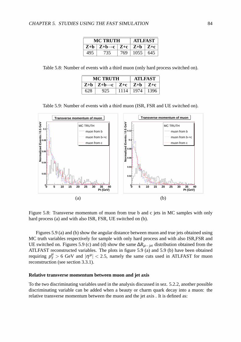
CHAPTER 5. STUDIES USING THE FAST SIMULATION 84
MC TRUTH ATLFASTZ+b Z+b→c Z+c Z+b Z+c495 735 769 1055 645
Table 5.8: Number of events with a third muon (only hard process switched on).
MC TRUTH ATLFASTZ+b Z+b→c Z+c Z+b Z+c628 925 1114 1974 1396
Table 5.9: Number of events with a third muon (ISR, FSR and UE switched on).
Pt (GeV)0 5 10 15 20 25 30 35 40
No
rmal
ized
Eve
nts
/ 0.
5 G
eV
0
0.02
0.04
0.06
0.08
0.1MC TRUTH
muon from b
muon from b->c
muon from c
Transverse momentum of muon
Pt (GeV)0 5 10 15 20 25 30 35 40
No
rmal
ized
Eve
nts
/ 0.
5 G
eV
0
0.02
0.04
0.06
0.08
0.1
0.12
MC TRUTH
muon from b
muon from b->c
muon from c
Transverse momentum of muon
(a) (b)
Figure 5.8: Transverse momentum of muon from true b and c jetsin MC samples with onlyhard process (a) and with also ISR, FSR, UE switched on (b).
Figures 5.9 (a) and (b) show the angular distance between muon and true jets obtained usingMC truth variables respectively for sample with only hard process and with also ISR,FSR andUE switched on. Figures 5.9 (c) and (d) show the same∆Rµ− jet distribution obtained from theATLFAST reconstructed variables. The plots in figure 5.9 (a)and 5.9 (b) have been obtainedrequiring pµ
T > 6 GeV and|η µ | < 2.5, namely the same cuts used in ATLFAST for muonreconstruction (see section 3.3.1).
Relative transverse momentum between muon and jet axis
To the two discriminating variables used in the analysis discussed in sez. 5.2.2, another possiblediscriminating variable can be added when a beauty or charm quark decay into a muon: therelative transverse momentum between the muon and the jet axis . It is defined as:

CHAPTER 5. STUDIES USING THE FAST SIMULATION 85
DeltaR0 0.05 0.1 0.15 0.2 0.25 0.3 0.35 0.4 0.45 0.5
No
rmal
ized
Eve
nts
/ 0.
02 D
elta
R
0
0.05
0.1
0.15
0.2
0.25
0.3
MC TRUTH
muon from b
muon from b->c
muon from c
Angular distance muon from jet
DeltaR0 0.05 0.1 0.15 0.2 0.25 0.3 0.35 0.4 0.45 0.5
No
rmal
ized
Eve
nts
/ 0.
02 D
elta
R
0
0.05
0.1
0.15
0.2
0.25
MC TRUTH
muon from b
muon from b->c
muon from c
Angular distance muon from jet
(a) (b)
DeltaR0 0.05 0.1 0.15 0.2 0.25 0.3 0.35 0.4 0.45 0.5
No
rmal
ized
Eve
nts
/ 0.
01 D
elta
R
0
0.05
0.1
0.15
0.2
0.25ATLFAST
muon from b
muon from c
Angular distance muon from jet
DeltaR0 0.05 0.1 0.15 0.2 0.25 0.3 0.35 0.4 0.45 0.5
No
rmal
ized
Eve
nts
/ 0.
01 D
elta
R
0
0.02
0.04
0.06
0.08
0.1
0.12
0.14
0.16
0.18
0.2
0.22
0.24
ATLFAST
muon from b
muon from c
Angular distance muon from jet
(c) (d)
Figure 5.9: Angular distance between muon and MC jet in the sample with only hard process (a)and with also ISR, FSR, UE switched on (b). Angular distance between muon and ATLFASTreconstructed jet in the sample with only hard process (c) and with also ISR, FSR, UE switchedon (d).
pRelT = |~pµ |sin(arccos(
~pµ · ~p jet
|~pµ || ~p jet|)) (5.3)
A schematic draft ofpRelT is shown in figure 5.10.
Due to the bigger mass of the b quark, muons from b jets show to have apRelT value greater
than muons from c jets, as it is shown in the plots in fig. 5.11 for both Monte Carlo truth andATLFAST.

CHAPTER 5. STUDIES USING THE FAST SIMULATION 86
Figure 5.10: Relative momentum (pRelT ) of muon respect to the jet axis.
For this analysis three variables were used to discriminateZ+b jet from Z+c jet events:
• ptrel : relative transverse momentum between muon and jet,
• masstracks: invariant mass of all the charged tracks inside a cone∆R= 0.4 from the jetaxis ,
• d0max: maximum impact parameter among all the charged tracks inside a cone∆R= 0.4from the jet axis.
Efficiency and rejection as a function of cuts on single variables, are shown in fig. 5.12.
The table 5.10 shows efficiency and rejection factor obtained combining cuts on two vari-ables amongpRel
T , d0maxandmasstracks, while the table 5.11 is obtained combining cuts onall the three parameters.
Summarizing the results, I can obtain a good efficiency of≈ 70% and purity of≈ 80%when cutting in the following ranges: 1≤ |d0max| ≤ 3 mm , 1.0≤ masstracks≤ 2.0 GeV and0.5≤ pRel
T ≤ 1.0 GeV.
Results from Multivariate Analysis
The variables used to train the three classifiers are the onesdescribed above.Since only a fraction of≈ 10 % of beauty and charm quark decay into muons, if I require
the precence of at least one non isolated muon (definied as in section 5.2.3), the sample will bereduced to a factor≈ 4-6 % of the initial sample. Due to a non sufficient sample of simulateddata, for this analysis I increased the statistics of the initial data samples to 350k events (hardprocess only).
The distributions of the input variables for signal and background are shown in figure 5.13.

CHAPTER 5. STUDIES USING THE FAST SIMULATION 87
Pt rel(GeV)0 1 2 3 4 5 6
No
rmal
ized
Eve
nts
/ 0.
1 G
eV
0
0.02
0.04
0.06
0.08
0.1
0.12
0.14
0.16
0.18MC TRUTH
muon from b
muon from b->c
muon from c
Relative momentum muon-jet
Pt rel(GeV)0 1 2 3 4 5 6
No
rmal
ized
Eve
nts
/ 0.
1 G
eV
0
0.02
0.04
0.06
0.08
0.1
0.12
0.14
0.16MC TRUTH
muon from b
muon from b->c
muon from c
Relative momentum muon-jet
(a) (b)
Pt rel(GeV)0 1 2 3 4 5 6
No
rmal
ized
Eve
nts
/ 0.
1 G
eV
0
0.02
0.04
0.06
0.08
0.1
0.12
0.14
0.16 ATLFAST
muon from b
muon from c
Relative momentum muon-jet
Pt rel(GeV)0 1 2 3 4 5 6
No
rmal
ized
Eve
nts
/ 0.
1 G
eV
0
0.02
0.04
0.06
0.08
0.1
0.12
0.14
0.16
ATLFAST
muon from b
muon from c
Relative momentum muon-jet
(c) (d)
Figure 5.11:pRelT between muon and MC true jet in the sample with only hard process (a) and
with also ISR, FSR, UE switched on (b).pRelT between muon and ATLFAST reconstructed jet
in the sample with only hard process (c) and with also ISR, FSR, UE switched on (d).
Figure 5.14 shows the correlations between the input variables.Figure 5.15 shows the classifier output distributions for signal and background events from
the test sample. By TMVA convention, signal (background) events accumulate at large (small)classifier output values. Hence, cutting on the classifier output, I can select the signal samplewith efficiencies and purities that respectively decrease and increase with the cut value. Theresulting relations between background rejection versus signal efficiency are shown in figure5.16 for all classifiers that were used in this work.
By a preliminary glance at the plots of figure 5.15, it is possible to see that the LikehoodEstimator is the best discriminating method, also if respect to the previous study with only two
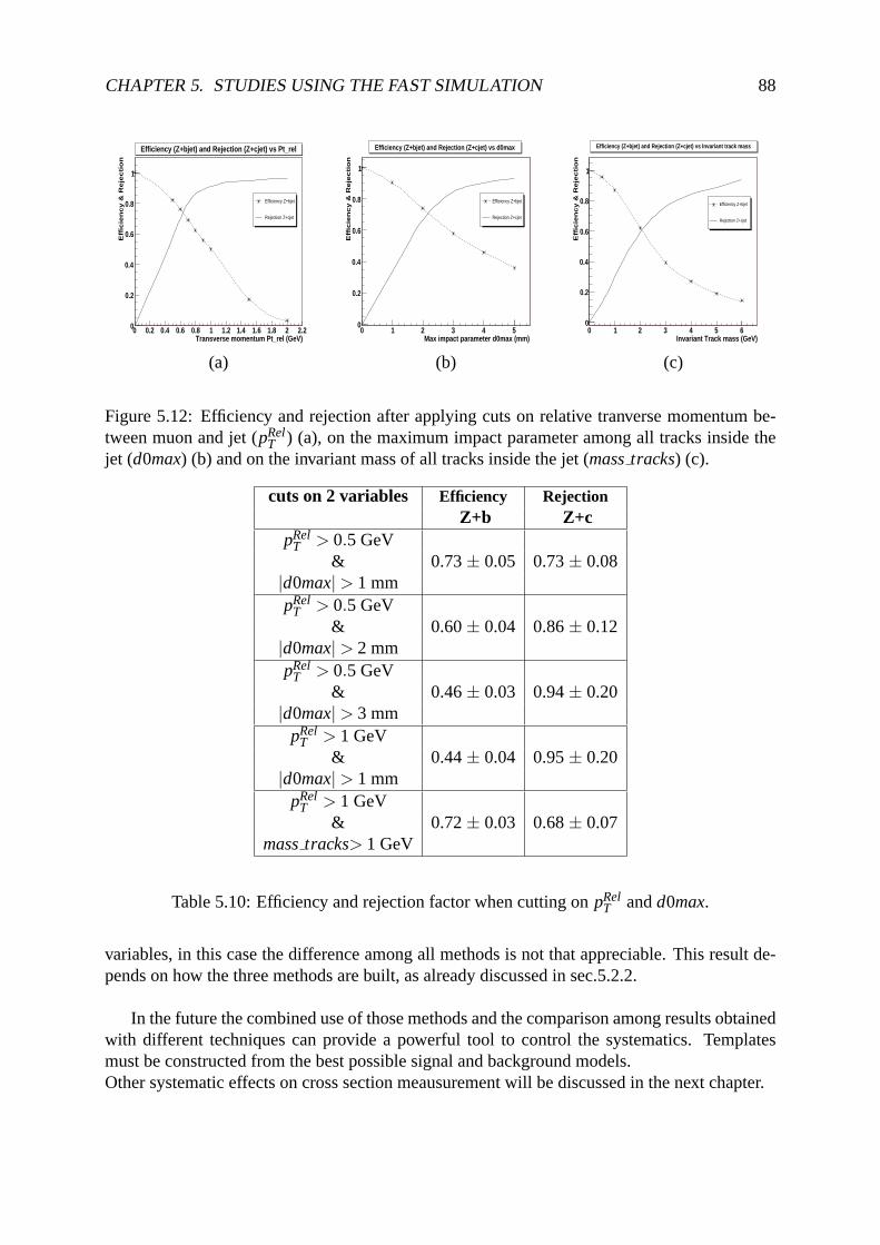
CHAPTER 5. STUDIES USING THE FAST SIMULATION 88
Transverse momentum Pt_rel (GeV)0 0.2 0.4 0.6 0.8 1 1.2 1.4 1.6 1.8 2 2.2
Eff
icie
ncy &
Reje
cti
on
0
0.2
0.4
0.6
0.8
1
Efficiency Z+bjet
Rejection Z+cjet
Efficiency (Z+bjet) and Rejection (Z+cjet) vs Pt_rel
Max impact parameter d0max (mm)0 1 2 3 4 5
Eff
icie
ncy &
Reje
cti
on
0
0.2
0.4
0.6
0.8
1
Efficiency Z+bjet
Rejection Z+cjet
Efficiency (Z+bjet) and Rejection (Z+cjet) vs d0max
Invariant Track mass (GeV)0 1 2 3 4 5 6
Eff
icie
ncy &
Reje
cti
on
0
0.2
0.4
0.6
0.8
1
Efficiency Z+bjet
Rejection Z+cjet
Efficiency (Z+bjet) and Rejection (Z+cjet) vs Invariant track mass
(a) (b) (c)
Figure 5.12: Efficiency and rejection after applying cuts onrelative tranverse momentum be-tween muon and jet (pRel
T ) (a), on the maximum impact parameter among all tracks inside thejet (d0max) (b) and on the invariant mass of all tracks inside the jet (masstracks) (c).
cuts on 2 variables Efficiency RejectionZ+b Z+c
pRelT > 0.5 GeV
& 0.73± 0.05 0.73± 0.08|d0max| > 1 mmpRel
T > 0.5 GeV& 0.60± 0.04 0.86± 0.12
|d0max| > 2 mmpRel
T > 0.5 GeV& 0.46± 0.03 0.94± 0.20
|d0max| > 3 mmpRel
T > 1 GeV& 0.44± 0.04 0.95± 0.20
|d0max| > 1 mmpRel
T > 1 GeV& 0.72± 0.03 0.68± 0.07
masstracks> 1 GeV
Table 5.10: Efficiency and rejection factor when cutting onpRelT andd0max.
variables, in this case the difference among all methods is not that appreciable. This result de-pends on how the three methods are built, as already discussed in sec.5.2.2.
In the future the combined use of those methods and the comparison among results obtainedwith different techniques can provide a powerful tool to control the systematics. Templatesmust be constructed from the best possible signal and background models.Other systematic effects on cross section meausurement will be discussed in the next chapter.

CHAPTER 5. STUDIES USING THE FAST SIMULATION 89
cuts on 3 variables Efficiency RejectionZ+b Z+c
pRelT > 0.5 GeV
& mass tracks> 0.5 GeV 0.71± 0.05 0.74± 0.09& |d0max| > 1 mm
pRelT > 0.5 GeV
& mass tracks> 1 GeV 0.66± 0.04 0.77± 0.09& |d0max| > 1 mm
pRelT > 0.5 GeV
& mass tracks> 2 GeV 0.49± 0.04 0.85± 0.12& |d0max| > 1 mm
pRelT > 0.5 GeV
& mass tracks> 3 GeV 0.32± 0.03 0.90± 0.15|d0max| > 1 mmpRel
T > 0.5 GeV& mass tracks> 2 GeV 0.41± 0.03 0.90± 0.15
& |d0max| > 2 mmpRel
T > 0.5 GeV& mass tracks> 0.5 GeV 0.45± 0.03 0.94± 0.19
& |d0max| > 3 mmpRel
T > 0.5 GeV& mass tracks> 1 GeV 0.55± 0.04 0.87± 0.13
& |d0max| > 2 mm
Table 5.11: Efficiency and rejection factor when cutting onpRelT , masstracksandd0max.
Figure 5.13: Input variable distributions to train the TMVAclassifiers.

CHAPTER 5. STUDIES USING THE FAST SIMULATION 90
-100
-80
-60
-40
-20
0
20
40
60
80
100
ptrel d0maxmassa_tracks
ptrel d0maxmassa_tracks
ptrel
d0max
massa_tracks
ptrel
d0max
massa_tracks
Correlation Matrix (signal)
100 0 19
0 100 0
19 0 100
linear correlation coefficients in %
-100
-80
-60
-40
-20
0
20
40
60
80
100
ptrel d0maxmassa_tracks
ptrel d0maxmassa_tracks
ptrel
d0max
massa_tracks
ptrel
d0max
massa_tracks
Correlation Matrix (background)
100 -2 29
-2 100 2
29 2 100
linear correlation coefficients in %
(a) (b)
Figure 5.14: Correlation between input variables: linear correlation coefficients for the signal(a) and background (b) training samples.

CHAPTER 5. STUDIES USING THE FAST SIMULATION 91
Likelihood0.1 0.2 0.3 0.4 0.5 0.6 0.7 0.8 0.9 1
Norm
alize
d
0
2
4
6
8
10
12
14
16
Likelihood0.1 0.2 0.3 0.4 0.5 0.6 0.7 0.8 0.9 1
Norm
alize
d
0
2
4
6
8
10
12
14
16SignalBackground
MVA output for method: Likelihood
Fisher-0.5 0 0.5 1 1.5 2
Norm
alize
d
0
0.2
0.4
0.6
0.8
1
1.2
1.4
1.6
1.8
2
2.2
Fisher-0.5 0 0.5 1 1.5 2
Norm
alize
d
0
0.2
0.4
0.6
0.8
1
1.2
1.4
1.6
1.8
2
2.2 SignalBackground
MVA output for method: Fisher
MLP
0.2 0.4 0.6 0.8 1 1.2
Norm
alize
d
0
0.5
1
1.5
2
2.5
3
3.5
4
MLP
0.2 0.4 0.6 0.8 1 1.2
Norm
alize
d
0
0.5
1
1.5
2
2.5
3
3.5
4 SignalBackground
MVA output for method: MLP
Figure 5.15: Classifier output distributions for signal and background events from the test sam-ple. Likelihood Estimator (upper plot), Fisher Discriminant (middle plot) and MLP-NeuralNet(bottom plot) are shown.

CHAPTER 5. STUDIES USING THE FAST SIMULATION 92
Signal efficiency0 0.1 0.2 0.3 0.4 0.5 0.6 0.7 0.8 0.9 1
Bac
kgro
un
d r
ejec
tio
n
0.5
0.55
0.6
0.65
0.7
0.75
0.8
0.85
0.9
0.95
1
Signal efficiency0 0.1 0.2 0.3 0.4 0.5 0.6 0.7 0.8 0.9 1
Bac
kgro
un
d r
ejec
tio
n
0.5
0.55
0.6
0.65
0.7
0.75
0.8
0.85
0.9
0.95
1
MVA Method:LikelihoodMLPFisher
Background rejection versus Signal efficiency
Figure 5.16: Background rejection versus signal efficiency obtained by cutting on the classifieroutputs for the events of the test sample.

Chapter 6
Systematics Uncertainties
The uncertainties on cross section measurement due to systematic effects have been neglectedin the analysis discussed in the previous chapters. Here I briefly discuss the major contributorsto the systematic uncertainty on Z→ µµ + b jet cross section measurement.
The primary concern arises from the determination of jet energy scale and estimation ofb-tagging efficiency and rejection, which may alter the sample composition significantly. Oneof the main theoretical uncertainties originates from the uncertainty on the parton content of theproton (PDF) that affect calculation of signal and background cross sections.
6.1 Jet Energy scale
Errors due to a miscalibration of the jet energy scale (JES) are expected to be one of the domi-nant systematics for the determination of Z (µµ) + b jet cross-section.The evaluation of JES uncertainty was done for theZ/W + jets channels [44, 65], in first ap-proximation we can consider that the obtained results do notchange much when we replace alight jet with a b jet.
If the energy is miscalibrated by a positive correction, more jets pass the selection cut andtherefore there will be more high multiplicity events and viceversa when the energy is miscali-brated by a negative correction.Figure 6.1 shows the relative systematic error on the ratio between measurement and theory forthe inclusive Z (e+e−) + jets cross section (a) and for the transverse momentum of the leadingjet (b) expected for different uncertainties on the Jet Energy Scale. Ratio of 1 correspond not tohave systematic uncertainties.ATLAS expects a limited precision on the jet energy scale in the first years, starting from un-certainties at the level of 10% and converging eventually towards 1% : 1% corresponding to theexperiment challenging goal, 3% turn-on expected value, 10% for the worst case. If 3% erroron JES is achived in early data, the systematic uncertainty on the inclusive cross section is atthe same level as the sum of all the other statistical and systematic uncertainties. In this case,the overall precision on the data/theory ratio expected with the first fb−1 of data is at the levelof 8-15% for topologie with 1-3 jets.In the worst scenario, a jet energy scale uncertainty of 10% results in the dominant error on the
93

CHAPTER 6. SYSTEMATICS UNCERTAINTIES 94
cross section. In this case, the total uncertainty on the cross section is at the level of 15-30%.But, if it is achieved the challenging uncertainty in JES of 1%, systematic errors decreases toless than 0.5 %.
Inclusive jet multiplicity1 2 3 4 5
Cro
ss s
ectio
n ra
tio u
ncer
tain
ty
0.2
0.4
0.6
0.8
1
1.2
1.4
PDF uncertainty
+ Unfolding, Backgrounds, Statistics
+ 3% Jet energy scale uncertainty
+ 10% Jet energy scale uncertainty
ATLAS
leading jet (GeV)TP50 100 150 200 250
Cro
ss s
ectio
n ra
tio u
ncer
tain
ty
0.2
0.4
0.6
0.8
1
1.2
1.4
PDF uncertainty
+ Unfolding, Background, Statistics
+ 3% Jet energy scale uncertainty
+ 10% Jet energy scale uncertainty
ATLAS
(a) (b)
Figure 6.1: Uncertainty on the ratio of measurement and theory for the inclusive jet cross-section (a) and thepT , of the leading jet (b) for theZ → e+e− + jets, process [44].
6.2 PDF
An important source of theoretical systematic uncertainties on cross sections measurements atthe LHC is represented by the Parton Distribution Functions(PDF). In the last years the PDF’sknowledge has largely improved mainly thanks to HERA [60]. This improvement reduces theerror on the Z + jets cross section calculations: each PDFs group now quotes uncertainties lowerthan 5%. The effect of such uncertainty on the on the ratio of measurement and theory for theinclusive Z (e+e−) + jets cross section and and for the transverse momentum of the leading jet,has been shown in figure 6.1. We can conclude that it becomes less important respect to othersystematic effects with the increasing of jets multiplicity and/or of the transverse momentumof the leading jet. Neverthless the estimation of above was realized using the CTEQ5 pdf set,using different sets it has been shown that they are in agreement within an error of∼ 8% [61,62].
Since at leading order the Z + b jet production can have originfrom the interaction of agluon and a b quark and because up to now the knowledge on the b content of the proton is lessprecise respect to the light quarks that can give origin to the Z + jets process [10], we expectthat the error on the cross section measurement due to the PDFuncertainty will increase of afew percent respect to the one quoted for the inclusive Z+jets channel.
CHAPTER 6. SYSTEMATICS UNCERTAINTIES 95
6.3 b-tagging algorithm
Vertex tagging of jets requires fine tuning of the inner detector performance. Determination ofthe b-tagging efficiency requires careful study of control samples. The b-tagging performancehas been studied for several physics channels considering different tagging algorithms [46].The contributions to the b tagging uncertainties have different origins: they come from theimpact of the tracker material on performance, the sensitivity to the calibration of tagging algo-rithms, the impact of the pixel detector conditions, the sensitivity to the Monte Carlo modelling.The overall impact is expected to be a 10-15% relative changein light jet rejection power. Theimpact on b tagging performance due to each contribution is discussed in detail in [46].
In section 4.5 I discussed a strategy to measure the mistagging rate directly from data usingthe W → µν inclusive sample that does not contain b-jet at the first order in perturbartiontheory. The result is that this method allows to keep the mistagging below a value of 5% for thegauge boson transverse momentum of. 100 GeV. So far no study in ATLAS has estimated theaccuracy with which fake rates can be measured. However, based on the Tevatron experience,it seems that a 10% relative error could be achievable with 100 pb−1.

Conclusions
The production of a Z boson together with jets containing heavy-quarks (c, b) is an impor-tant signal at the hadron colliders. In this analysis I have presented a feasibility study of theproduction ofZ bosons decaying to muons in association with b-jets performed with a set ofsimulated signal and background Monte Carlo samples corresponding to an integrated luminos-ity of 1fb−1.
This channel will serve as one of the Standard Model benchmarks for physics analyses aswell as Beyond Standard Model signals. Furthermore, it represents a clear and high statisticschannel to perform studies on the b parton content of the proton (PDF). The precise measure-ment of Z + b jet cross section will help in reducing the current uncertainty on the partoniccontent of the proton. Such uncertainty is presently affecting the potential for discovering newphysics at LHC.In order to measure the cross section when the experiment will start to take data, we need tohave a good control of the possible background and of the principal sources of systematic uncer-tainties. The main aim of this work has been to develop analysis techniques in order to evaluatethe contamination of the signal from backgrounds and to study possible methods to extract sig-nal from such backgrounds.
Z → µµ + b jet events suffer from two different kind of backgrounds.The first consists ofevents not containing a Z that decay into a muon pair, but involving muons in the final state thatpass the isolation criteria appearing as muons from Z boson.In association to muons at leastone jet is reconstructed and identified as a beauty jet. Theseevents are:tt events involving atleast one semileptonic decay in muon, Z→ ττ events with subsequentτ decay into muon, W→ µν with a second muon coming from a jet or a second fake muon and QCDmulti-jet eventsfiltered to favour the presence of real muons or hadrons misidentified as muons (bb events). Thesecond originates from events containing a Z boson decayinginto a muon pair (as the signal),but with a c or light jet mis-identified as a beauty jet. These are Z (µµ) + c/light jet events.It has been shown that the former, except QCD (bb) jets production, can be reliably estimatedfrom current Monte Carlo predictions, although in situ verification with data will be needed.bbbackground dealing with rare fluctuations of large cross section processes can only be crudelyestimated from current Monte Carlo simulation. With the selection cuts used in the analysispresented in this work we expect to select the signal events with an efficiency of of∼ 40%for an integrated luminosity of 1fb−1, corresponding to a few months of running at moderateluminosity (0.3nb−1s−1). The dominant contribute to the background comes from jetsproduc-tion in QCD processes (bb). The backgrounds fromtt ,Z → ττ , W → µν and Z + light jet arenegligible, while the contamination from Z + c jet should be of the order of 10−30% . The
96

CHAPTER 6. SYSTEMATICS UNCERTAINTIES 97
main limitation to the background estimation comes from thelimited statistic of the availableMonte Carlo samples, especially the QCD (bb) sample: after selection cuts only a few eventsremain and the statistical error is really big. In order to better estimate the contamination of thesignal due to this background further studies are required with larger MC samples. Neverthless,I showed that it is possible to reduce the percentage from this background optimizing cuts onthe variables and exploiting different methods to distinguish signal from background (like fit onthe di-muon pair invariant mass). In addition, Tevatron experience [47, 48] make us confidentthat real data will help in improving the discrimination between signal and QCD (bb) jets back-ground. In such scenario one of the main backgrounds to be reduced is from Z + c jet eventswhere the c is mistagged as a b jet.The second part of this work concerned the study of a strategyto reduce this background re-ducing the mistagging rate of c jets. Two different methods for tagging of b jets have beenconsidered, which allow for the selection of samples with different levels of efficiency and pu-rity: the first is based on the impact parameter of tracks associated to the jet and on the invariantmass of these tracks, the second includes also the transverse relative momentum between muonand jet for events containing a third muon coming from the semi leptonic decay of a B hadroninside the b jet. In the latter case the suppression of the background is certainly better, but thestatistic sample is strongly reduced. In both cases I investigated the potential of different tech-niques and I showed that is possible to have a better discrimination (especially for the case witha third muon) using a Multivariate Analysis.With the first method (impact parameter and invarian mass b tagging) it is possible to reach asignal efficiency in selecting Z+ b jet event of≈ 70% a rejection factor of background eventsof ≈ 60%, while with the second method (soft muon tagging) the efficiency is≈ 90% and therejection is≈ 60%.The first method can be useful in a first phase when the statistic will be quite small, while thesecond (which exploit the third muon in the event) can be usedwhen the statistic will be im-proved.In the future the combined use of those methods and the comparison among results obtainedwith different techniques can provide a powerful tool to control the systematics and templatesmust be constructed from the best possible signal and background models.Furthermore, I have investigated the possibility to control the mistagging rate directly fromdata. The b-tagging efficiency can be controlled by looking at the number of tagged jets in datasamples that in principle should not contain b jets at first order, like W + jets events. What Ihave shown is that we expect a mistagging rate per event belowthe 5% over the fullpT rangeof the signal.
The uncertainties on signal efficiency and background contamination in the selected sampledue to systematic effects have been neglected in this analysis, but important elements of thesystematic errors that will affect the cross section measurement of the Z→ µµ + b jet channelhave been enumerated and discussed. The main contributors to systematic uncertainties comefrom the determination of jet energy scale, the estimation of b-tagging efficiency and rejectionand from the uncertainty on the parton content of the proton (PDF). The overall systematicuncertainty on cross section measurement considering these three contributors is expected to bebetween 15% and 30% depending essentially from the performance and the knowledge of theATLAS experiment.
Acknowledgements
Il primo grazie va ai miei genitori per avermi aiutata a crescere, a sognare e a capire che le aspi-razioni possono essere realizzate, basta crederci davvero! Questo dottorato nee una delle prove.
Un sentito ringraziamentoe rivolto al Prof. Filippo Ceradini che in questi anni di dottoratomi ha dato la possibilita di continuare ad ampliare le conoscenze nel mondo della fisicalasciando che io seguissi i miei interessi e le mie inclinazioni scientifiche sia per cio che riguardala mia formazione che la realizzazione di questo lavoro.Un profondo grazie va alla Professoressa Fernanda Pastore che mi ha seguita passo dopo passodurante tutto il periodo della mia formazione universitaria, dagli anni di laurea fino al terminedi questo dottorato:grazie per il supporto ma anche per l’affetto.Grazie alle Dott.sse Ada Farilla, Monica Verducci ed Alessandra Tonazzo che hanno collabo-rato con me nelle varie fasi di realizzazione di questa tesi con dedizione ed entusiasmo.Voglio ringraziare il Dott. Carlo Carloni Calame per essere riuscito con la sua calma e pazienza,ma anche con la sua simpatia a fare un po’ di chiarezza nel buiomundo dei generatori MonteCarlo, il Dott. Iacopo Vivarelli per l’aiuto nelle prime fasidi utilizzo del software di simu-lazione veloce dell’esperimento(ATLFAST) e il Dott. Federico Nguyen per avermi introdottosulla misteriosa strada dell’analisi multivariata.Un graziee indirizzato a tutto il gruppo di ricerca di ATLAS di Roma Tre:alla Dott.ssaDomizia Orestano, al Dott. Toni Baroncelli, al Dott. Mauro Iodice e al Dott. Fabrizio Petrucciper avermi dato la la possibilita di “divagare un po’ ” dalla fisica dei dati simulati per approc-ciarmi alla fisica delle calibrazioni delle camere a deriva dello spettrometro a muoni. Tra tuttiloro un particolare ringraziamento va a Fabrizio per i suoi consigli e incoraggiamenti anche neimomenti di maggiore difficolta: grazie per la prontezza e la pazienza!Un ringraziamento di cuore alla Dott.ssa Manuela Cirilli chee sempre stata il mio punto diriferimento al CERN: grazie per il tempo dedicatomi, ma soprattutto per la cioccolata che haallietato i miei turni di notte di presa dati di raggi cosmiciin Control Room!
Un sincero grazie va agli amici che hanno condiviso con me questi anni di dottorato: aSimona-Thelma per le avventure vissute insieme e per la travolgente e contagiosa risata, aValentino per il suo rincuorante “buongioooorno” seguito dallo “scambiamoci un po’ di af-fetto” capace di rallegrare le giornate, a Massimiliano perla caparbieta nel cercare di offrirmicaffe su caffe (ci sono voluti quasi 3 anni pero alla fine ho accettato!), a Gabriele per il suo“pessimismo cosmico” che non mi ha mai fatto sentire sola, a Cristian e a Luca per averpiacevolmente accorciato le giornate in acquario con pausedi chiacchiere e sorrisi, a Fabiolache nonostante la distanza resta sempre l’amica con cui condividere le (dis)avventure del mondodella fisica.
98

CHAPTER 6. SYSTEMATICS UNCERTAINTIES 99
Uno speciale ringraziamento va a Roberto per la pazienza nel rispondere ai miei SOS di naturateorica (forse ora mie piu chiaro cosa sia una scala di fattorizzazione!), ma soprattutto “pertutto il resto”.
Grazie a Marina, la mia migliore amica, per essermi stata sempre accanto, anche nei mo-menti di dubbi e perplessita nei quali mi sono imbattuta durante questi anni di dottorato: seidavvero una amica speciale!Un particolare grazie va a Filippo per essermi stato sempre ecomunque vicino con morbidiabbracci e rincuoranti parole.
Questi anni di studio e lavoro sono stati allietati da scuolee conferenze nelle quali hoampliato l’orizzonte delle mie conoscenze sia nel campo della fisica che in quello delle amicizie!E’ per questo che voglio ringraziare tutte le ragazze e i ragazzi con cui ho potuto confrontarmie con i quali ho condiviso una parte di questo mio percorso. Ungrazie speciale va a Nico-letta per le giornate passate insieme tra uffici, control room, caffetteria del CERN e... relais del’entrecote, a Diego per le impagabili risate, a Rossella peril suo ottimismo e la sua allegria.
Le giornate all’universita non sarebbero certo state le stesse se non avessi potuto condi-viderle con tutti i miei “figli e nipoti” dell’aula 27! Non puo mancare un ringraziamento aisegretari Alessandra e Andrea per i mille favori!!!La tenacia nel portare avanti questo lavoroe anche il frutto dell’affetto di tanti altri amici e par-enti: grazie a Elena, Milena, Agnese, Alessandra, Andrea, Arianna, Caterina, Raffaella, MariaRosaria, Daniela, Stefano, Giulio, Maria, Erika e Attilio.Almost last (but not least) I want to thank Moustapha for his help in writing the thesis, butespecially for his contagious optimism.
Colgo in ultimo l’occasione per ringraziare tutti quelli chelottano e protestano per garantireil diritto allo studio e alla ricerca:e anche grazie a chi crede nel progresso scientifico e necapisce l’importanza che questo lavoroe stato possibile.

Bibliography
[1] W.-M. Yao et al.Journal of Physics, G 33, 1, 2006, http://pdg.web.cern.ch/pdg/pdg.html
[2] C.Quigg Gauge Theories of the Strong, Weak and Electromagnetic Interactions. , TheBenjamin/Cummings Publishing Company, London, 1983
[3] P.Higgs Phys.Lett.,12:132, 1964
[4] F.Englert and R.Brout Phys. Rev. Lett. 13: 321-23, 1964
[5] G. Guralnik, C. R. Hagen and T. W. B. Kibble Phys. Rev. Let. 13: 585-87, 1964
[6] S.Martin hep-ph, 9709356, 1999
[7] G.Altarelli, G.Parisi, Nucl. Phys. B126, 289, 1977
[8] S.Dawson, hep-ph ,9612229 ,1997
[9] R.K. Ellis, W.J. Stirling and B.R. Webbwr,QCD and Collider Physics, CambridgeMonographs on Particle Physics, Nuclear Physics and Cosmology, 1996
[10] R.K. Ellis, W.J. Stirling and B.R. Webber,Hard interactions of quarks and gluons: aprimer for LHC physicsRep.Prog.Phys, 70, 89-193, 2007
[11] D. Boussardet al., The Large Hadron Collider Conceptual Design Report,CERN/AC,95-05, 1995
[12] http://lepewwg.web.cern.ch/LEPEWWG/
[13] [ATLAS Collaboration],The ATLAS Experiment at the CERN Large Hadron Collider,2008 JINST 3 S08003
[14] [ATLAS Collaboration],ATLAS Forward Detectors for Measurement of Elastic Scatter-ing and Luminosity, CERN/LHCC/2008-004
[15] [CDF Collaboration]Charged jet evolution and the underlying event in proton anti-proton collisions at 1.8-TeV, Phys.Rev. D, 56, 2002, 092002.
[16] [CDF Collaboration],The underlying event in hard interactions at the Tevatron anti-p pcollider, Phys.Rev. D, 70, 2004, 072002, [arXiv:hep-ex/0404004]
100
BIBLIOGRAPHY 101
[17] J. Campbell, R. K. Ellis, F. Maltoni and S. Willenbrock,Higgs-Boson Production inAssociation with a Single Bottom Quark, Phys. Rev.D 67 (2003) 095002 [arXiv:hep-ph/0204093]
[18] J. Campbell, F. Maltoniet al., Higgs Boson Production in Association with BottomQuarksPhys. Rev., 2004, arXiv:hep-ph/0405302
[19] J. Campbell, R. K. Ellis, F. Maltoni and S. Willenbrock,Associated Production of aZ Boson and a Single Heavy-Quark Jet, Phys. Rev. D 69, 074021, 2004, [arXiv:hep-ph/0312024]
[20] Fermi National Accelerator Laboratoryhttp://www.fnal.gov
[21] The LEP Collaboration Aleph, Delphi, L3, OPAL Collaborations and the LEP Elec-troweak working groupPrecision Electroweak Measurements and Constraints on theStandard ModelCERN-PH-EP/2007-039, arXiv:0712.0929
[22] https://twiki.cern.ch/twiki/bin/view/Atlas/WorkBookAthenaFrameworkhttps://twiki.cern.ch/twiki/bin/view/Atlas/WorkBookPackages.
[23] https://twiki.cern.ch/twiki/bin/view/Atlas/AthenaReleaseshttps://twiki.cern.ch/twiki/bin/view/Atlas/ReleaseRecipeshttp://atlas-computing.web.cern.ch/atlas-computing/projects/releases/status/.
[24] T. Sjostrand, S. Mrenna and P. Skands,High Energy Physics Event Generation withPYTHIA6.1,JHEP05 (2006) 026, (LU TP 06-13, FERMILAB-PUB-06-052-CD-T) [hep-ph/0603175].
[25] T. Gleisberg, S. Hoche, F. Krauss, A. Schalicke, S. Schumann, J. Winter, JHEP, 0402,056,2004
[26] G. Corcella, I.G. Knowles, G. Marchesini, S. Moretti, K.Odagiri, P. Richardson, M.H.Seymour and B.R. Webber,HERWIG 6.5,JHEP, 0101-010, 2001; [hep-ph/0011363],[hep-ph/0210213]
[27] M.L. Mangano, M. Moretti, F. Piccinini, R. Pittau, A.D. Polosa, JHEP, 0307, 001, 2003
[28] S. Frixione, B. R. Webber,The MC@NLO 3.2 Event Generator,CERN-PH-TH, 2006-012, 2006;
[29] J. Campbell, R.K. Ellis,http : //mcfm.fnal.gov/;J. Campbell, R.K. Ellis, Phys. Rev.D65 113007 (2002).
[30] J.Allison et al., Geant4 developments and applicationsIEEE Transaction on NuclearScience, 53(1):270-278, 2006
[31] C.Alexaet al. Geant4 hadronic physics validation with LHC test-beamdata: first con-clusions.CERN-LCGAPP, 10, 2004
[32] [ATLAS Computing Group],Technical design report, ATLAS TDR, 2005

BIBLIOGRAPHY 102
[33] D. Adams et al.,Track Reconstruction in the ATLAS Muon Spectrometer with MOORE,ATLAS Note, ATL-SOFT-2003-007, 2003.
[34] Th. Lagouri et al,A Muon Identification and Combined Reconstruction Procedurefor theATLAS detector at CERN LHC, IEEE Trans.Nucl.Sci., 51 (2004) 3030-3033.
[35] S.Hassini,et al., NIM A572, 77-79, 2007
[36] S. D. Ellis, J. Huston, K. Hatakeyama, P. Loch and M. Tonnesmann, Prog. Part. Nucl.Phys.60, 484 (2008) [arXiv:0712.2447 [hep-ph]].
[37] M. Cacciari and G. P. Salam, Phys. Lett. B641, 57 (2006) [arXiv:hep-ph/0512210].
[38] A. Abulencia et al. [CDF - Run II Collaboration], Phys. Rev. D75, 092006 (2007)[Erratum-ibid. D75, 119901 (2007)] [arXiv:hep-ex/0701051].
[39] D.Cavalliet al., Performance of the ATLAS fast simulation ATLFASTATLAS Note, com-phys-012, 2007
[40] R.Lefevre, C.In situ determination of the scale and resolution of the jet energy measure-ments using Z0 + jets events, ATLAS Internal Note, ATL-PHYS-2002-026, 2002
[41] J. Proudfoot,et al., Jet Energy Scale Calibration in Vector Boson Events using RomeSimulation Data, ATLAS Internal Note, ATL-COM-PHYS-2005-067, 2005
[42] [ATLAS Collaboration]Jet and Missing Et Combined Performance CSC ChapterATL-COM-PHYS-2008-074
[43] [ATLAS Collaboration],ATLAS reference cross-section note, ATL-COM-PHYS, 2008-077, 2008;
[44] [ATLAS Collaboration]Standard Model CSC NoteATL-COM-PHYS-2008-064
[45] S. Correardet al., b-tagging with DC1 data, ATL-PHYS-2004-006, (2004)
[46] [ATLAS Collaboration]b-tagging CSC chapterATL-COM-INDET-2008-011
[47] [The DO Collaboration], DO Note 4388, Phys. Rev. Lett.94161801 (2005);
[48] [CDF Collaboration],Measurement of the b Jet Cross Section in Events with a Z Bosonin pp Collisions at
√s= 1.96TeV, hep-ex/0605099, May 2006
[49] V. M. Abazov et al. [D0 Collaboration],A measurement of the ratio of inclusive crosssectionσ(pp→ Z+b jet)/σ(pp→ Z+ jet) at
√s= 1.96TeV, [arXiv:hep-ex/0410078],
(26 Oct 2004)
[50] J. Pumplin, D.R. Stump, J. Huston, H.L. Lai, P. Nadolsky,W.K. Tung,New Generationof Parton Distributions with Uncertainties from Global QCD Analysis, hep-ph/0201195,JHEP07, 012, 2002;
[51] A.D.Martin et al., MRST2001: partons and alphaS from precise deep inelastic scatteringand Tevatron jet data,Eur.Phys.J ,C23,73, 2002, [hep-ph/0110215]
BIBLIOGRAPHY 103
[52] A.D.Martin et al., Physical Gluons and High ET Jets[hep-ph/0410230]
[53] S.Chekanovet al., ZEUS next-to-leading-order QCD analysis of data on deep inelasticscattering, Phys.Rev.D67, 012007, 2003 ;
[54] J. M. Campbell, J. W. Huston and W. J. Stirling, Rept. Prog.Phys. 70, 89 (2007);
[55] A.Hoeckeret al., TMVA, Toolkit for Multivariate Data Analysis with ROOT.CERN-OPEN-2007-007, June 2007, [arXiv physics/0703039]
[56] R.Brunet al., ROOT An Object-Oriented Data Analysis FrameworkUser Guide
[57] http://atlas-sw.cern.ch/cgi-bin/viewcvs-atlas.cgi/offline/Generators/DC3joboptions/share/
[58] http://projects.hepforge.org/lhapdf/
[59] C.Adloff et al., Measurement and QCD analysis of neutral and charged current crosssections at HERAEur. Phys. J,C30, 1, 2003;[hep-ex:0304003]
[60] S.Alekhinet al., HERA and the LHC - A workshop on the implications of HERA for LHCphysics,CERN, 2005-014, 2006; [hep-ph/0511119v1]
[61] A. Tricoli, A. Cooper-Sarkar, C.Gwenlan,Uncertainties on W and Z production at theLHC CERN, 2005-014, 2005; [hep-ex:0509002]
[62] M.Bellomo, C.Carloni Calame, S. Diglio, M.Malberti, C.Rovelli W,Z and pdf’s mea-surements with early data in ATLAS and CMSNuovo Cimento B 123 3-4 (2008), DOI:10.1393/ncb/i2008-10554-2
[63] M. Cacciari, E. Laenen, S. Diglio, A. Tonazzo, M. Verducci et. al. Theoretical re-view of various approaches in heavy quark production, CERN-2005-014 (14 December2005)[arXiv:hep-ph/0601012-3]
[64] S.Diglio, A.Farilla, A.Tonazzo, M.Verducci,Associated production of a Z boson and ab-jet in ATLASATL-PUB-PHYS, 2007-014, 2007; [hep-ex:0710.4461]
[65] E.DobsonW/Z+jets studies in ATLASATL-COM-PHYS-2008-091