
THERMAL MODELLING OF HIGH SPEED MACHINE TOOL...
91
THERMAL MODELLING OF HIGH SPEED MACHINE TOOL SPINDLES By: TURGUT KÖKSAL YALÇIN Submitted to the Graduate School of Engineering and Natural Sciences in partial fulfillment of the requirements for the degree of Master of Science Sabanci University 2015
Transcript of THERMAL MODELLING OF HIGH SPEED MACHINE TOOL...
THERMAL MODELLING OF HIGH SPEED MACHINE TOOL SPINDLES
By:
TURGUT KÖKSAL YALÇIN
Submitted to the Graduate School of Engineering and Natural Sciences in partial
fulfillment of the requirements for the degree of
Master of Science
Sabanci University
2015

THERMAL MODELLING OF HIGH SPEED MACHINE TOOL SPINDLES
APPROVED BY:
Prof. Erhan BUDAK ........................................
(Thesis Advisor)
Assoc. Prof. Mustafa BAKKAL ........................................
Assoc. Prof. Bahattin KOÇ ........................................
Date of Approval:

© Turgut Köksal YALÇIN 2015
All Rights Reserved

To my family

v
TERMAL MODELLING OF HIGH SPEED MACHINE TOOL SPINDLES
Turgut Köksal Yalçın
Industrial Engineering, MS Thesis, 2015
Thesis Supervisor: Prof. Dr. Erhan Budak
Keywords: High Speed Spindle, Spindle Thermal Growth, Thermal Error
Modelling, FEM, Cooling System Analysis
Abstract
Machining is the most widely used manufacturing method by far since its
foundation and its development process still continues parallel to the technology.
Demand for higher quality parts together with the lower machining time and cost is
rapidly increasing. In order to meet this increasing demand, high speed machining
processes and equipment are getting much more important compared to the traditional
methods. High speed machine tools are the key elements of this new machining era; but
making the machine tools faster while improving their overall performance requires
high end technology together with advanced engineering applications. Positioning
accuracy of a high speed machine tool is the most important metric among others
because of its direct effect on the finished parts, which are measured as dimensional
errors. The highly strong and nonlinear relationship between the positional accuracy and
the thermal characteristics of the machine tools raises the importance of modeling the
thermal behavior of the machine tools.
The main aim of this thesis is to develop robust thermal models for high speed
machine tool spindles, by considering the effects of built-in cooling systems, to be able
to predict and then reduce the positioning errors related to the thermal behavior of the
spindle unit. Fully analytical approaches are very complex for solving the nonlinear
thermal behavior of the spindle units; but they are still powerful when they used
together with the finite elements model of the complex spindle geometry. As the first
step of the thermal model, the heat generated by the ball bearings, which is considered
as the main heat source of the entire spindle unit, is calculated analytically. Calculated

vi
heat is used as an input to the Finite Elements Method (FEM) model for the heat
transfer and thermal error calculations. Built-in cooling system of the spindle unit is
also analyzed using the Computational Fluid Dynamics (CFD) approaches again using
FEM models. Overall temperature distributions and thermal elongations leading to
positioning errors are calculated by the FEM model. Simulation results are validated by
temperature and thermal elongation experiments measured on a 5-axis CNC machine
tool spindle. Cooling system parameters optimization is achieved by using the
developed models as quick solutions to the positioning problems. On the other hand
cooling system design improvements are also analyzed by the developed models and
several different cooling channel designs are investigated for increasing the positioning
accuracy of the high speed machine tool spindle used in the experiments. Overall good
agreement is observed between experiments and simulations.

vii
YÜKSEK HIZLI İŞ MİLLERİNİN TERMAL MODELLENMESİ
Turgut Köksal Yalçın
Endüstri Mühendisliği, Yüksek Lisans Tezi, 2015
Tez Danışmanı: Prof. Dr. Erhan Budak
Anahtar Kelimeler: Yüksek Hızlı İş Mili, İş Mili Termal Uzaması, Termal Hata
Modellemesi, Sonlu Elemanlar Analizi, Soğutma Sistemi Analizi
Özet
Talaşlı imalat, bulunuşundan bu yana en çok tercih edilen imalat yöntemlerinin
başında gelmekte ve ilerleyen teknoloji ile paralel olarak gelişimini sürdürmektedir.
Daha hassas toleranslara sahip parçaların daha hızlı, daha kaliteli ve daha ucuza
üretilmesi yönündeki talep gün geçtikçe artmaktadır. Artan bu talebin karşılanabilmesi
için geleneksel yöntemlere nazaran yüksek hızlı işleme yöntemleri ve ekipmanları daha
da önem kazanmaktadır. Talaşlı imalatın yeni döneminin kilit elemanları olan yüksek
hızlı takım tezgâhları, işleme hızı ile birlikte genel performans artışı sağlayabilmek
adına en son teknolojiler ve yenilikçi mühendislik uygulamaları kullanılarak
geliştirilmektedir. Geleneksel takım tezgâhlarında olduğu gibi yüksek hızlı tezgâhlarda
da pozisyonlama hassasiyeti son parça boyutlarına doğrudan yansıdığı ve boyutsal
hatalar doğurduğu için tezgâh değerlendirme kriterleri arasındaki en önemli faktördür.
Pozisyonlama hassasiyetinin tezgâhların termal karakteristikleri ile son derece kuvvetli
ve karmaşık ilişkisi, yüksek hızlı takım tezgâhlarındaki termal davranışların
modellenmesinin önemini arttırmaktadır.
Bu tez çalışmasının amacı, yüksek hızlı iş millerinde sıcaklığa bağlı oluşan
pozisyonlama hatalarının doğru tahmin edilebilmesi ve azaltılabilmesi için iş mili
üzerindeki dahili soğutma sistemi etkilerini de göz önünde bulunduran termal
modellerin oluşturulmasıdır. Zamana bağlı ve lineer olmayan sıcaklık denklemlerinin
kompleks geometriler ile birlikte tamamen analitik yöntemlerle çözümü son derece zor
olduğundan; sonlu elemanlar yöntemine baş vurulmuştur. İş mili sıcaklık kaynaklarının
en önemlisi olan iş mili bilyalı yataklarının ürettiği ısı miktarı analitik olarak
hesaplanması modelin ilk adımıdır. Hesaplanan ısılar iş mili sonlu elemanlar
modeline(SEM) aktarılarak iş mili elemanları arasındaki ısı transferleri ve bu transferler

viii
sonucu oluşan termal uzamalar hesaplanmıştır. İş milinde bulunan dahili soğutma
sistemi, akışkanlar dinamiği çözümleri için yine sonlu elemanlar analizi kullanılarak
incelenmiştir. Isı kaynakları ve soğutma sistemleri sonucu oluşan sıcaklık dağılımları ve
termal uzamalardan kaynaklanan pozisyonlama hataları SEM kullanılarak
hesaplanmıştır. Oluşturulan modele ait simülasyon sonuçları 5 eksenli CNC takım
tezgahı üzerinde yapılan sıcaklık ve termal uzama testleri ile doğrulanmıştır.
Pozisyonlama hatalarına pratik bir çözüm olarak soğutma sistemine ait parametrelerin
iyileştirilmesi yine oluşturulan modeller üzerinden yapılmıştır. Soğutma sistemi dizayn
iyileştirmesi yönünde farklı kanal geometrilerinin iş mili sıcaklık dağılımına ve
pozisyonlama hatalarına olan etkileri simülasyonlar aracılığı ile incelenmiştir.
Simülasyon ve test sonuçlarının birbirine yakın olduğu gözlenmiştir.

ix
ACKNOWLEDGEMENTS
I would like to express the deepest appreciation to my thesis advisor Prof. Erhan Budak
for his guidance, patience and supports. His dedication to his job and motivation for the
research always impressed me. I learned a lot from his wise point of view against any
situation and valuable thoughts about life.
I would like to thank my committee members Assoc. Prof. Bahattin Koç and Assoc.
Prof. Mustafa Bakkal for their grateful assistance and suggestions to my project.
I would also like to thank each member of the Manufacturing Research Laboratory
(MRL) family, especially to my friends Cihan Özener, Ekrem Can Unutmazlar, Mert
Kocaefe, Batuhan Yastıkçı, Mehmet Albayrak, Gözde Bulgurcu, Samet Bilgen, Hayri
Bakioğlu, Faraz Tehrenizadeh, Zahra Barzegar for their continuous support on every
issue.
I greatly appreciate the assistance of the Maxima R&D members, Dr. Emre Özlü, Esma
Baytok, Veli Nakşiler, Anıl Sonugür, Ahmet Ergen, Tayfun Kalender and Dilara
Albayrak, everything will be harder without their assistance and experience.
I am also indebted to Spinner Machine Tools for providing the research tools, which my
entire research was based on and thankful to Muharrem Sedat Erberdi for sharing his
valuable experience with me.
Finally, I would like to thank TÜBİTAK (Scientific and Technological Research
Council of Turkey) for supporting me financially throughout my project by granting a
scholarship.
Last but not least, I am most thankful to my family Asuman Köksal and Hakkı Reşit
Yalçın for their limitless support throughout my entire life. Nothing would be possible
without their sacrifice and patience. I dedicate this work to them.
x
1. TABLE OF CONTENTS
2. INTRODUCTION ........................................................................................................ 1
2.1 Introduction and Literature Survey ......................................................................... 1
2.2 Objective ................................................................................................................. 5
2.3 Layout of the Thesis ................................................................................................ 6
3. BEARING HEAT GENERATION .............................................................................. 7
3.1 Introduction ............................................................................................................. 7
3.2 Friction Torque and Heat Due to Applied Load ..................................................... 7
3.3 Friction Torque Due to Viscosity of the Lubricant ............................................... 11
3.4 Calculation of the Convective Heat Transfer Coefficients ................................... 16
3.5 Summary ............................................................................................................... 18
4. FINITE ELEMENTS MODEL OF THE SPINDLE UNIT ........................................ 19
4.1 Introduction ........................................................................................................... 19
4.2 Cooling System Model (CFX-CFD) ..................................................................... 19
4.3 Thermal Model ...................................................................................................... 28
4.4 Static Structural Model ......................................................................................... 29
4.5 Model Simulations ................................................................................................ 31
a) Cooling Water Temperatures ........................................................................... 31
a) Spindle Shaft Temperatures ............................................................................. 31
a) Spindle Surface Temperatures ......................................................................... 32
b) Deflections of the Tool Tip .............................................................................. 36
4.6 Summary ............................................................................................................... 36
5. EXPERIMENTAL RESULTS AND VERIFICATION OF THE SPINDLE
THERMAL MODEL ...................................................................................................... 39
5.1 Introduction ........................................................................................................... 39
5.2 Experimental Set-up .............................................................................................. 39
5.3 Constant Spindle Speed Tests Results .................................................................. 44
5.3.1 Longer Duration Tests .................................................................................... 44
5.3.2 Shorter Duration Tests .................................................................................... 49
5.4 Variable Spindle Speed Test Results .................................................................... 52
5.5 Comparison of Shorter Duration Constant Spindle Speed Test Results and FEM
Simulations .................................................................................................................. 54
a) Temperature Comparisons ............................................................................... 55
b) Comparisons of the Tool Tip Deflections ........................................................ 55
5.6 Identification of the Tool Tip Deflection Sources ................................................ 56
5.7 Summary ............................................................................................................... 59

xi
6. COOLING SYSTEM OPTIMIZATIONS .................................................................. 60
6.1 Introduction ........................................................................................................... 60
6.2 Parameter Optimizations ....................................................................................... 60
a) Effect of Cooling Fluid Velocity ...................................................................... 61
b) Effect of Cooling Fluid Temperature ............................................................... 62
6.3 Design Optimization ............................................................................................. 64
a) Axial Cooling Channels ................................................................................... 65
b) Cooling Channels with Lower Helix Angle and Unified Diameter ................. 67
6.4 Summary ............................................................................................................... 69
7. SUGGESTIONS FOR FURTHER RESEARCH ....................................................... 71
8. DISCUSSIONS AND CONCLUSIONS .................................................................... 73
REFERENCES ............................................................................................................... 75
xii
LIST OF FIGURES
Figure 3. 1: Angular contact ball bearing (Source: Schaeffler) ........................................ 8
Figure 3. 2: Calculations of load ratio and equivalent static loads ................................. 10
Figure 3. 3: Friction torque due to applied load ............................................................. 10
Figure 3. 4: Heat generation due to applied load 7011 ................................................... 11
Figure 3. 5: Heat generation due to applied load 7014 ................................................... 12
Figure 3. 6: Viscous friction torque ................................................................................ 13
Figure 3. 7: Heat generated due to viscous friction ........................................................ 14
Figure 3. 8: Total generated heat for 7011 ...................................................................... 14
Figure 3. 9: Total generated heat for 7014 ...................................................................... 15
Figure 3. 10: Mass properties of the bearings ................................................................. 15
Figure 3. 11: Heat distribution of the bearings ............................................................... 16
Figure 3. 12: Convective heat transfer coefficients of the spindle shaft ......................... 18
Figure 4. 1: Cooling unit of the investigated machine tool ............................................ 20
Figure 4. 2: Subsystems available in ANSYS ................................................................ 21
Figure 4. 3: 3D CAD model of the spindle components used in the model ................... 22
Figure 4. 4: ANSYS modules used in the model ............................................................ 23
Figure 4. 5: Meshed version of the spindle housing and shaft ....................................... 23
Figure 4. 6: Pre-defined regions of the spindle unit used in the model .......................... 24
Figure 4. 7: Outline of the spindle CAD model used in CFX module ........................... 26
Figure 4. 8: Model tree of the CFX module ................................................................... 27
Figure 4. 9: 3D CAD models of the overall spindle unit used in the thermal module ... 28
Figure 4. 10: Imported Loads ......................................................................................... 29
Figure 4. 11: Example results of the Static Structural Module ....................................... 30
Figure 4. 12: Temperature of the cooling fluids within the cooling channels for different
spindle speeds ................................................................................................................. 33
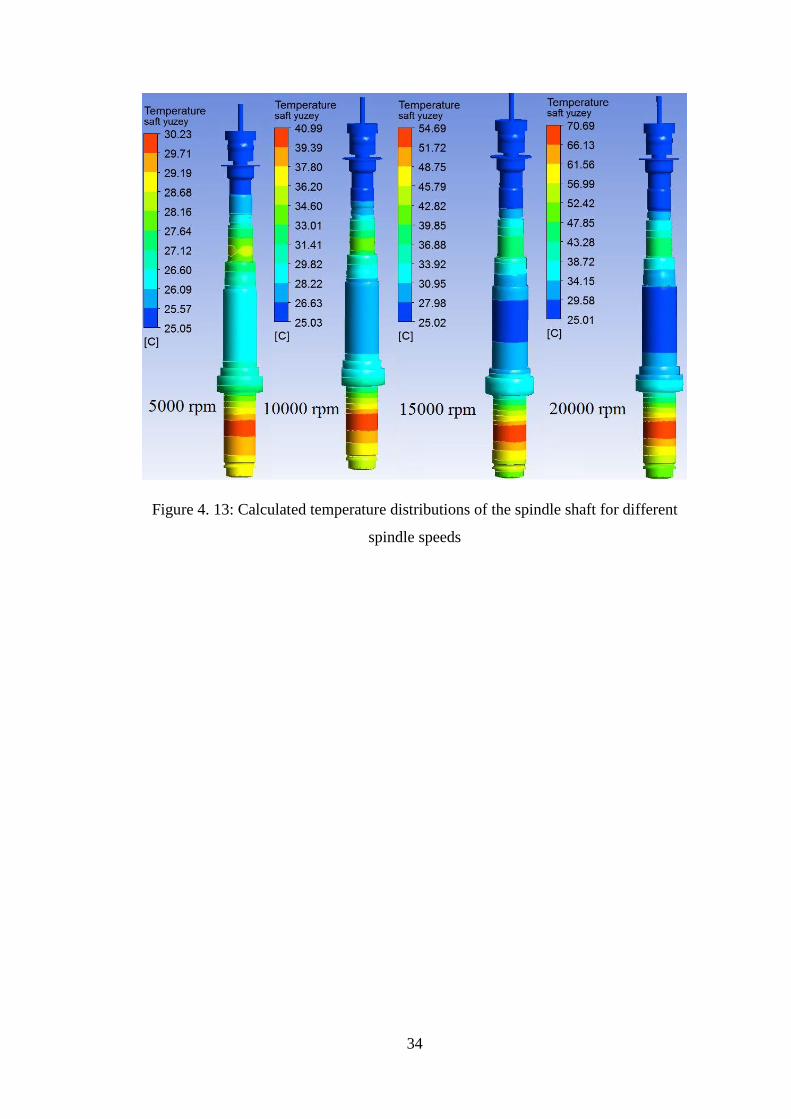
Figure 4. 13: Calculated temperature distributions of the spindle shaft for different
spindle speeds ................................................................................................................. 34
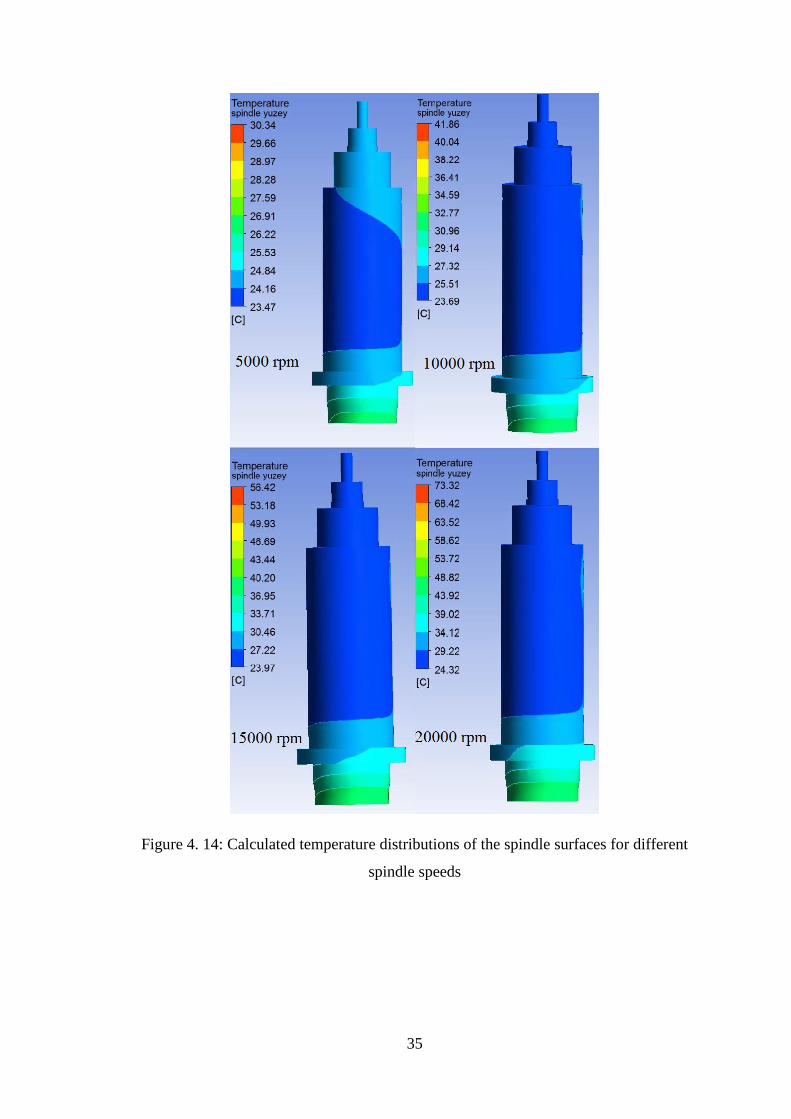
Figure 4. 14: Calculated temperature distributions of the spindle surfaces for different
spindle speeds ................................................................................................................. 35
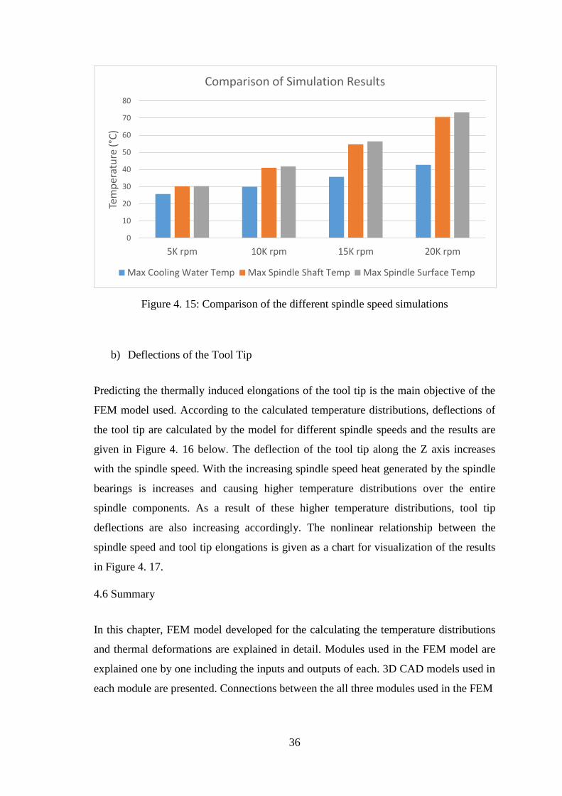
Figure 4. 15: Comparison of the different spindle speed simulations ............................ 36
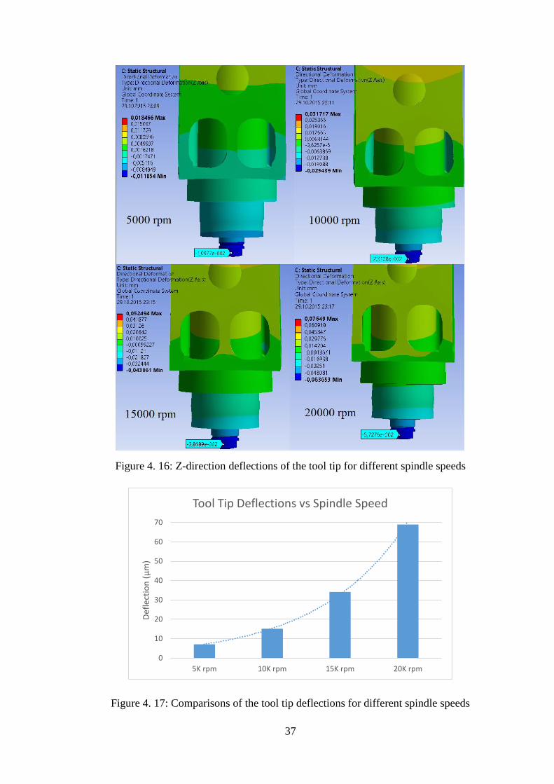
Figure 4. 16: Z-direction deflections of the tool tip for different spindle speeds ........... 37
Figure 4. 17: Comparisons of the tool tip deflections for different spindle speeds ........ 37
Figure 5. 1: FLIR A325 Infrared camera used in the measurements .............................. 41
xiii
Figure 5. 2: Example of a temperature measurement file ............................................... 41
Figure 5. 3: NCDT series displacement sensors ............................................................. 42
Figure 5. 4: Displacement measurement set-up and fixtures .......................................... 43
Figure 5. 5: IR camera images of the measured temperatures ........................................ 45
Figure 5. 6: Temperature plot of the heating phase ........................................................ 45
Figure 5. 7: Post-processed deflection measurement results of the heating phase ......... 46
Figure 5. 8: Schematic of the bending motion along Y direction ................................... 47
Figure 5. 9: Temperature plot of the cooling phase ........................................................ 48
Figure 5. 10: Post-processed deflection measurement results of the cooling phase ....... 48
Figure 5. 11: Temperature measurements of the shorter duration tests .......................... 49
Figure 5. 12: Graph of the shorter duration test results .................................................. 50
Figure 5. 13: Deflection results of the shorter duration tests .......................................... 51
Figure 5. 14: Comparison of results according to spindle speeds .................................. 51
Figure 5. 15: Deflection statistics of the short duration tests .......................................... 52
Figure 5. 16: Spindle speed profile presented in ISO 230-3 ........................................... 53
Figure 5. 17: Temperature results of the variable spindle speed tests ............................ 53
Figure 5. 18: Displacement results of the variable spindle speed tests ........................... 54
Figure 5. 19: Comparison of temperatures for experiments and simulation results ....... 55
Figure 5. 20: Deflection comparisons of different spindle speeds ................................. 56
Figure 5. 21: Identification tests, set-up and displacement sensor positions .................. 57
Figure 5. 22: Displacement results of the identification tests ......................................... 58
Figure 5. 23: FEM simulation result for identification tests in Z direction deflections. 59
Figure 6. 1: Comparison of different fluid velocities for the deflections ....................... 62
Figure 6. 2: Comparison of different fluid velocities for the temperatures .................... 62
Figure 6. 3: Comparison of different fluid initial temperatures for the deflections ........ 63
Figure 6. 4: Comparison of different fluid initial temperatures for the temperatures .... 64
Figure 6. 5: Axial cooling channels ................................................................................ 66
Figure 6. 6: Comparison of default cooling channels with axial cooling channels ........ 66
Figure 6. 7: Temperature distribution of the axial cooling channels .............................. 67
Figure 6. 8: Lower helix cooling channel geometry ....................................................... 68
Figure 6. 9: Lower- unified helix simulation results ...................................................... 69
Figure 6. 10: Comparison of default cooling channels with lower helix cooling channels
........................................................................................................................................ 70

xiv
LIST OF TABLES
Table 3. 1: z and y values of different bearing types ........................................................ 9
Table 3. 2: Values of fo for different bearing types ........................................................ 12
1
CHAPTER 2
2. INTRODUCTION
2.1 Introduction and Literature Survey
Machining is still the most commonly used manufacturing method for high
accuracy- critical to operation parts of the aerospace and defense industries; even
though it is one of the oldest methods. Machining technology is continuously
developing with the new requirements and demands of these two industries. New
materials, design methodologies and treatments are tightening the part quality
specifications so that machine tool technologies need continuous updates in order to
meet these specifications. CNC machine tool manufacturers are trying to optimize their
products by changing mechanical designs, materials used for the components,
outsourced components and control algorithms. Overall performance of a machine tool
can only be improved if all the contributors to the machine tool error term are improved
together. Positioning accuracy on the other hand is one of the most important aspects of
a CNC machine tool due to its direct effect on the finished parts. Major factors affecting
the machining and positioning accuracies of the machine tools are:
- Cutting forces generated by the cutting tool,
- Nonlinear heat, generated by both the cutting operation and electrical
components throughout the machine tool running time,
- Inaccuracies of the components due to manufacturing and assembling stages,
- Environmental temperature and heat sources,
- Errors due to the control system of the machine tool.
Among all these important factors, heat generation and the geometrical errors related to
this generated heat are responsible up to %75 of the total machine tool errors [1]. Heat
2
generation mechanism of the machine tools are complicated due to the time dependency
and non-linear behavior of the heat sources that contribute to the overall heat
generation; such as axis motors, linear guideways, ball screws, spindle motor and
bearings. Fully analytical computation of the heat generated in these sources is so hard
that mathematical models are developed for estimating the heat values. Estimating the
heat generated by all these components is still not enough to calculate the overall
temperature distribution and thermal deformations, because of the complicated machine
tool designs that are composed of different components and sub systems. The crucial
effects of thermal errors are fully recognized after the inaccuracies due to the
mechanical design and assembling technologies are minimized by the developed
technology in machine tool industry. Researchers found that eliminating only the
physical errors in machine tools is enough to produce parts with tighter tolerances.
Bryan is well known by his studies about thermal effects in both machine tool
technologies and metrology between 1963 and 1985. He published several papers about
the thermal effects in dimensional measurements [2], cutting tool thermal elongations
while chip removal [3] and machine tool spindle growth due to temperature rise [4].
Most of these primary studies are based on measuring temperature changes together
with dimensional measurements of tools or devices in order to link both results.
Thermal error studies of the machine tools mainly focused on the compensation of the
thermally induced errors. Zhang et al [5] studied error compensation techniques for the
coordinate measuring machines; he used rigid body kinematics and quick axis
measurements to compensate positioning errors of the CMMs first, then applied same
methodology to the machine tools. Weck [6,7] presented several direct and indirect
compensation methods starting with lathes and then for the machine tools in general. He
used the simple inputs such as motor currents, spindle speeds and environmental speeds
to estimate the thermally induced errors. Dönmez et al. [8] also worked on error
compensation for both measuring machines and machine tools; he used 3 step feature
based measurement technique to identify error mechanisms. Moriwaki et al. [9] focused
on the thermally induced errors of the spindle units specifically. He investigated the
effect of the environmental temperature on the spindle thermal errors for the ultra-
precision air spindle systems.
Thermal performances of the machine tools are investigated component vise due to the
high number of components which are contributing the overall heat generation. The
3
most important component of a machine tool for thermal behavior is the spindle unit.
High speed rotational movement used for chip removal is generated at the spindle unit
and due to frictional losses during this generation of the rotational movement heat is
generated [10]. Main contributors of the generated heat in the machine tool spindles are:
Spindle bearings
Spindle motor
Cutting operation
Modelling of the machine tool temperatures was always being a hot topic for the
researchers. Several approaches are used for the thermal performance studies, such as
analytical modeling techniques; which are developed to estimate the amount of heat
generated during the process using mathematical equations and physical theories; and
mapping techniques; which are used to create meaningful linkages between the
measured temperatures and measured thermal deformations. Most of the early studies
are categorized as mapping techniques. Some of the popular approaches used in these
kinds of studies are multiple-linear regression methods, artificial neural networks, grey
system theory, fuzzy logic systems. Regression analysis is still used in the recent
studies; Chen et al. [11] used basic linear regression analyses to compensate for the
thermally induced errors of a double column machining center. Wang et al. [12] used
the regression method to estimate thermal growth of the precision cutter grinders. He
established a compensation map by interpolating the results of several experiments by
regression method. Li et al. [13] developed a thermal compensation algorithm using
auto-regressive models so that he could directly calculate the compensation coefficients
from the NC code generated to manufacture parts. Artificial neural networks are used
very often for mapping the temperature and deflection measurements. By constructing a
smart training data, which contains possible scenarios and inputs to the systems, these
methods can estimate the outputs of a system to an unknown input successfully. Hattori
et al.[14] constructed a three layer feed forward neural net structure to estimate the
relationship between environmental temperatures and thermal displacements of a
vertical milling tool. Vanherck et al. [15] used artificial neural network with a single
layer 4-neuron model to estimate and compensate thermally induced errors of a 5-axis
milling machine. He reduced the maximum deformations of the tool tip from 150µm to
15µm with the proposed method. Mize and John [16] applied neural networks based

4
modelling approach together with kinematic error measurement method to a 3-axis
machine tool concluding in a 7µm of three dimensional positioning accuracy.
Analytical modeling techniques are for spindle thermal performance is studied by many
researchers; main aim of these studies is to predict thermally induced errors by
mathematical calculations and theories beforehand in order to compensate them. For the
analytical modeling techniques, spindle bearings are the most studied sources of thermal
performance researches. First and still widely used analytical method for predicting the
spindle temperatures was found by Palmgren [17]. He used rolling friction theory to
model the heat generation mechanism in spindle bearings and assumed that the bearings
are the only heat sources in the system. Rolling friction theory presented by Palmgren
was developed by Harris [18]; gyroscopic moments of the bearing balls are added to the
system. He also worked on bearing stability and provided a handbook for proper
bearing selection together with bearing life-time estimations. First one dimensional heat
transfer of the Palmgren’s bearing heat equations are presented by Burton and Staph
[19]. Jorgensen [20] constructed a quasi-three dimensional heat transfer network for
spindle temperature analysis by considering the bearings and motor as the main heat
sources. Stein and Tu [21], by combining the bearing heat model developed by Harris
with a more complex analytical heat transfer equations, they calculated the temperature
distribution of a spindle unit. By the addition of heat generated in spindle motor,
Bossmanns and Tu [22, 23] presented a new power flow model for estimating the
spindle temperature distribution. Another study based on the heat generation at the
spindle bearings was done by Li and Shin [24]; they investigated the effects of bearing
configurations on both thermal and dynamical aspects of the spindle units. Mostly used
bearing configurations are studied and compared according to the results of the thermo-
mechanical model presented in the paper. Thermo-mechanical models for bearings are
also developed by Li and Shin [25, 26] using the finite element approaches. Spindle
shaft, motor and bearings are divided in small elements for calculations of dynamical
behavior and thermal interactions. Conduction of heat from motor and bearings are
calculated iteratively by following the finite elements method. Thermal expansions of
the individual components are estimated. Min et al. [27] presented a detailed thermal
model especially for spindle bearings by using the initial approaches of Bossmanns and
Tu. They included the thermal contact resistance in their calculations of the heat
generation at the spindle bearings. They implemented the improved thermal model of
5
the previous versions on a grinding machine with a conventional spindle bearing.
Thermal expansions of the overall system are also calculated using their model. Jin et
al. [28] used the internal load distribution of the angular contact ball bearings to
calculate the heat generation. Frictional and sliding torques within the bearing balls and
raceways are added to the bearing thermal model presented by Harris [18]. Effects of
the external loads on the bearing temperatures are also included in their model.
The bearing heat generation model used in this study is the one presented by Harris
[18]; even though his modeling approach is empirical it is still the most widely used
approach by researchers. Harris considered all types of bearings while generating his
data set during 1973; including the state of the art, high speed angular contact bearings
with ceramic balls inside. These ceramic ball bearings were used in the aerospace
applications in that time and started to be used in the machine tool industry by the early
90s. Considering the fact that the design of the angular contact bearings haven’t been
changed much after their foundation, recent studies about the machine tool bearings are
still using Harris’s [25,27,28,37] model for heat predictions. The cooling systems and
materials on the other hand are the rapidly developing technologies for the thermal
problems of the machine tool industry compared to the almost mature bearing
technologies.
2.2 Objective
Thermal modelling of spindle units is quite important for improving the accuracies of
machine tools. In case of 5 axis high speed spindle units used in high precision
manufacturing applications of aviation and defense industries, thermal issues are the
main reasons of scrap parts. Constructing a thermal model for estimating the thermal
deformations of the machine tools accurately is very important for both machine tool
builders and machine tool users. Such models can be used by machine tool builders in
the design stages to reduce the thermal dependencies by better material selection,
thermally robust designing and avoiding excess heat generations. These models can also
be used by machine tool users for compensating the thermal errors by predicting them
beforehand. The ease of usage is a crucial parameter for industrial applications, instead
of just mathematical equations or lines of codes, providing visual feedback of
temperatures and deformations will be more effective for all users. Implementing such a

6
model based on 3D CAD data will be useful for designers to easily test the thermal
performances of their prototypes leading them to optimize their designs instantly.
The objective of this thesis is to come up with an industrial methodology; which can
accurately and robustly estimate the temperature distributions, heat sources, cooling
systems and finally the thermally induced errors of a high speed 5 axis machine tool
spindle unit; so that both machine tool builders-end users can easily use to monitor
thermal performances of their machine tools and optimize their designs or strategies.
2.3 Layout of the Thesis
The organization of this thesis is as follows:
In Chapter 2, high speed spindles and geometry of the bearings used in these spindles
are explained. Finite elements methods of thermal modeling together with the bearing
heat generation assumptions are presented.
In Chapter 3, bearing heat generation formulas are presented with the calculated heat
values for the bearings used in the spindle unit modeled. Effect of spindle speed and
bearing preloads are discussed. Methodology used for the heat partitioning is explained.
Heat transfer coefficients for the convection are also explained in this chapter.
In Chapter 4, FE model of the spindle unit is presented together with the solid models
and inputs. Different modules of the FE software, ANSYS, are explained in detail with
example results.
In Chapter 5, verification tests for the FE model are explained. Comparison of the
results from FE model developed and measurements done in the laboratory are shown.
Performance of the developed model for estimating the temperature distribution and
thermal deformations are discussed.
In Chapter 6, optimization of the cooling system parameters and geometry based on the
developed thermal model is presented. Results of these optimizations are shown and
compared to the current cooling systems results.
In Chapters 7 and 8, suggestions for the further research and discussions are presented.
7
CHAPTER 3
3. BEARING HEAT GENERATION
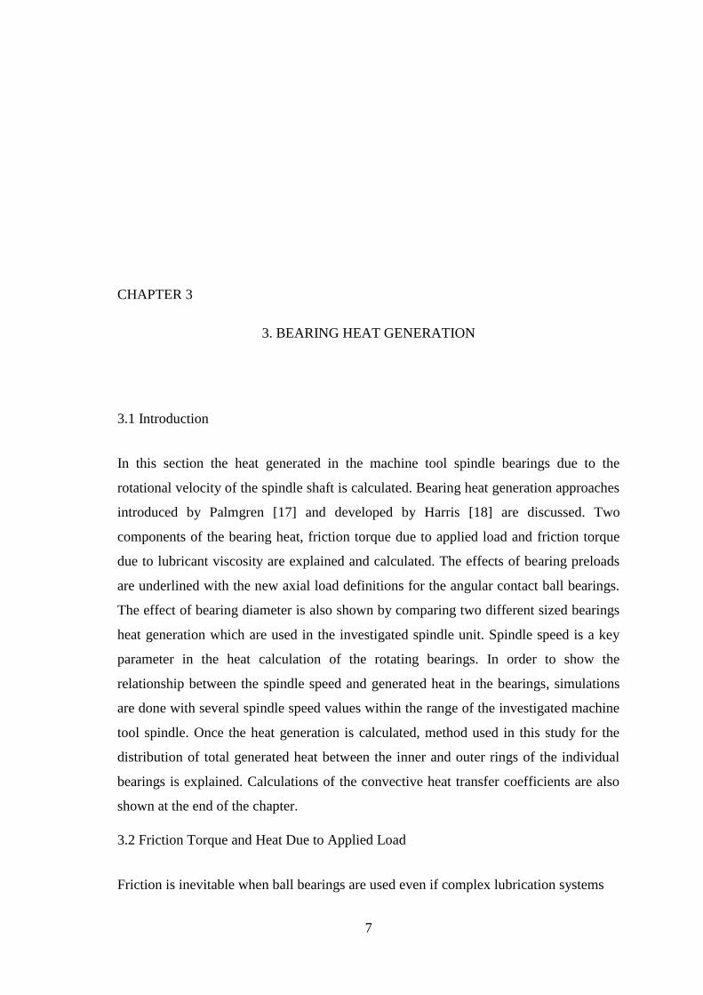
3.1 Introduction
In this section the heat generated in the machine tool spindle bearings due to the
rotational velocity of the spindle shaft is calculated. Bearing heat generation approaches
introduced by Palmgren [17] and developed by Harris [18] are discussed. Two
components of the bearing heat, friction torque due to applied load and friction torque
due to lubricant viscosity are explained and calculated. The effects of bearing preloads
are underlined with the new axial load definitions for the angular contact ball bearings.
The effect of bearing diameter is also shown by comparing two different sized bearings
heat generation which are used in the investigated spindle unit. Spindle speed is a key
parameter in the heat calculation of the rotating bearings. In order to show the
relationship between the spindle speed and generated heat in the bearings, simulations
are done with several spindle speed values within the range of the investigated machine
tool spindle. Once the heat generation is calculated, method used in this study for the
distribution of total generated heat between the inner and outer rings of the individual
bearings is explained. Calculations of the convective heat transfer coefficients are also
shown at the end of the chapter.
3.2 Friction Torque and Heat Due to Applied Load
Friction is inevitable when ball bearings are used even if complex lubrication systems
8
and fluids are used. In case of the rolling bearings, the continuous friction force
generated within the bearing assembly creates a friction torque in the negative direction
to the rotation of the spindle shaft. This friction torque is the main reason of the energy
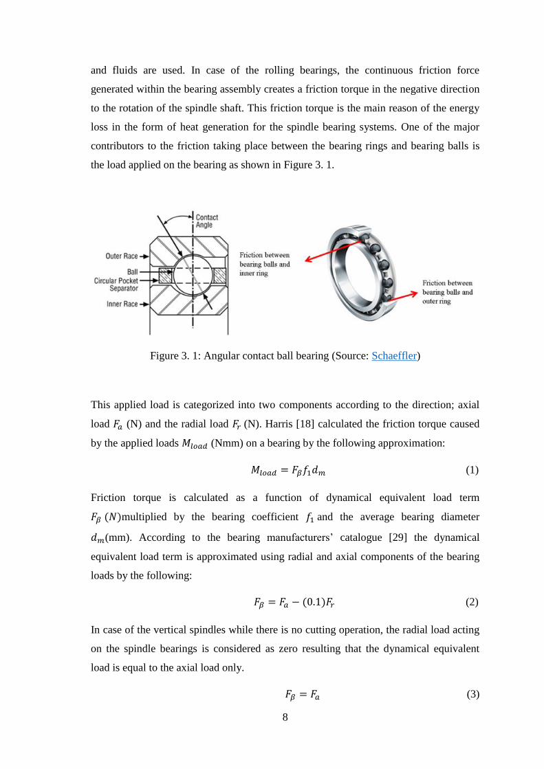
loss in the form of heat generation for the spindle bearing systems. One of the major
contributors to the friction taking place between the bearing rings and bearing balls is
the load applied on the bearing as shown in Figure 3. 1.
Figure 3. 1: Angular contact ball bearing (Source: Schaeffler)
This applied load is categorized into two components according to the direction; axial
load 𝐹𝑎 (N) and the radial load 𝐹𝑟 (N). Harris [18] calculated the friction torque caused
by the applied loads 𝑀𝑙𝑜𝑎𝑑 (Nmm) on a bearing by the following approximation:
𝑀𝑙𝑜𝑎𝑑 = 𝐹𝛽𝑓1𝑑𝑚 (1)
Friction torque is calculated as a function of dynamical equivalent load term
𝐹𝛽 (𝑁)multiplied by the bearing coefficient 𝑓1 and the average bearing diameter
𝑑𝑚(mm). According to the bearing manufacturers’ catalogue [29] the dynamical
equivalent load term is approximated using radial and axial components of the bearing
loads by the following:
𝐹𝛽 = 𝐹𝑎 − (0.1)𝐹𝑟 (2)
In case of the vertical spindles while there is no cutting operation, the radial load acting
on the spindle bearings is considered as zero resulting that the dynamical equivalent
load is equal to the axial load only.
𝐹𝛽 = 𝐹𝑎 (3)
9
In this study, axial load component of an angular contact ball bearing is calculated as
the combination of bearing preload values 𝐹𝑝𝑟𝑒𝑙𝑜𝑎𝑑 (N) together with the gravitational
force due to shaft weight 𝐹𝑔𝑟𝑎𝑣𝑖𝑡𝑦 (N). Since there is no cutting operation, cutting forces
are all assumed to be zero. With this new definition of the axial load components, the
effect of the bearing preload on the overall bearing heat generation is identified. The
axial load of an angular contact ball bearing is calculated as the following:
𝐹𝑎 = 𝐹𝑝𝑟𝑒𝑙𝑜𝑎𝑑 + 𝐹𝑔𝑟𝑎𝑣𝑖𝑡𝑦 (4)
The bearing coefficient term (𝑓1) used in the torque calculations is a factor depends on
the bearing design and bearing loads. It is calculated by the following formula:
𝑓1 = 𝑧(𝑃𝑜
𝐶0)𝑦 (5)
Parameters 𝑃𝑜 and 𝐶0 are the bearing dependent static equivalent load and basic static
load ratings respectively, while z and y values for various bearing types are calculated
by Harris [18] and given in Table 3. 1. Values of 𝐶0 are given in the bearing catalogues,
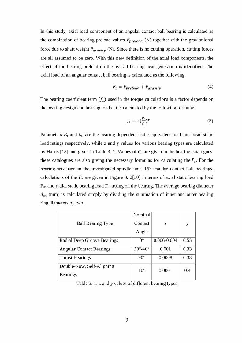
these catalogues are also giving the necessary formulas for calculating the 𝑃𝑜. For the
bearing sets used in the investigated spindle unit, 15° angular contact ball bearings,
calculations of the 𝑃𝑜 are given in Figure 3. 2[30] in terms of axial static bearing load
F0a and radial static bearing load F0r acting on the bearing. The average bearing diameter
𝑑𝑚 (mm) is calculated simply by dividing the summation of inner and outer bearing
ring diameters by two.
Ball Bearing Type
Nominal
Contact
Angle
z y
Radial Deep Groove Bearings 0° 0.006-0.004 0.55
Angular Contact Bearings 30°-40° 0.001 0.33
Thrust Bearings 90° 0.0008 0.33
Double-Row, Self-Aligning
Bearings 10° 0.0001 0.4
Table 3. 1: z and y values of different bearing types
10
Figure 3. 2: Calculations of load ratio and equivalent static loads
Contact angles of the bearings are selected according to the application and loading, the
only influential parameter for bearing selection is the load ration of axial to radial loads
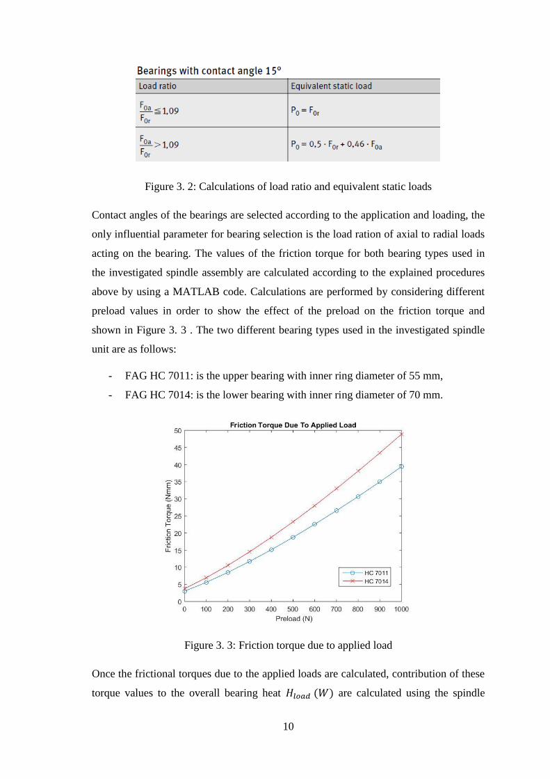
acting on the bearing. The values of the friction torque for both bearing types used in
the investigated spindle assembly are calculated according to the explained procedures
above by using a MATLAB code. Calculations are performed by considering different
preload values in order to show the effect of the preload on the friction torque and
shown in Figure 3. 3 . The two different bearing types used in the investigated spindle
unit are as follows:
- FAG HC 7011: is the upper bearing with inner ring diameter of 55 mm,
- FAG HC 7014: is the lower bearing with inner ring diameter of 70 mm.
Figure 3. 3: Friction torque due to applied load
Once the frictional torques due to the applied loads are calculated, contribution of these
torque values to the overall bearing heat 𝐻𝑙𝑜𝑎𝑑 (𝑊) are calculated using the spindle
11
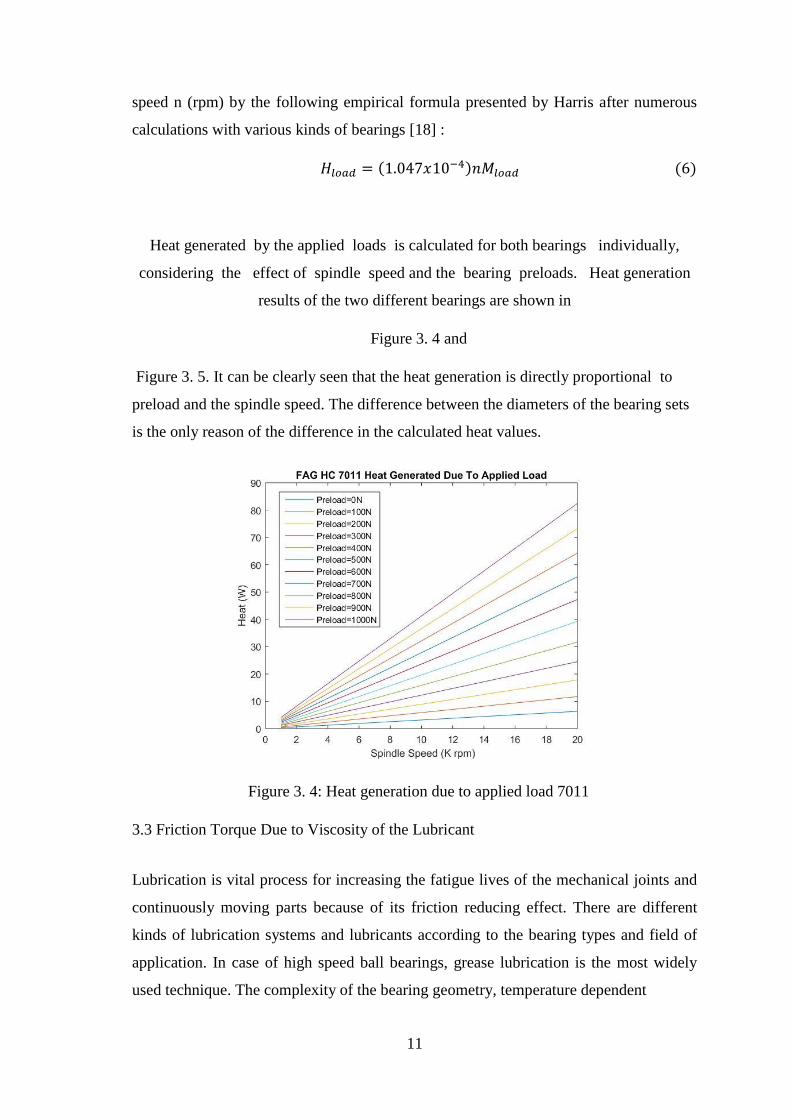
speed n (rpm) by the following empirical formula presented by Harris after numerous
calculations with various kinds of bearings [18] :
𝐻𝑙𝑜𝑎𝑑 = (1.047𝑥10−4)𝑛𝑀𝑙𝑜𝑎𝑑 (6)
Heat generated by the applied loads is calculated for both bearings individually,
considering the effect of spindle speed and the bearing preloads. Heat generation
results of the two different bearings are shown in
Figure 3. 4 and
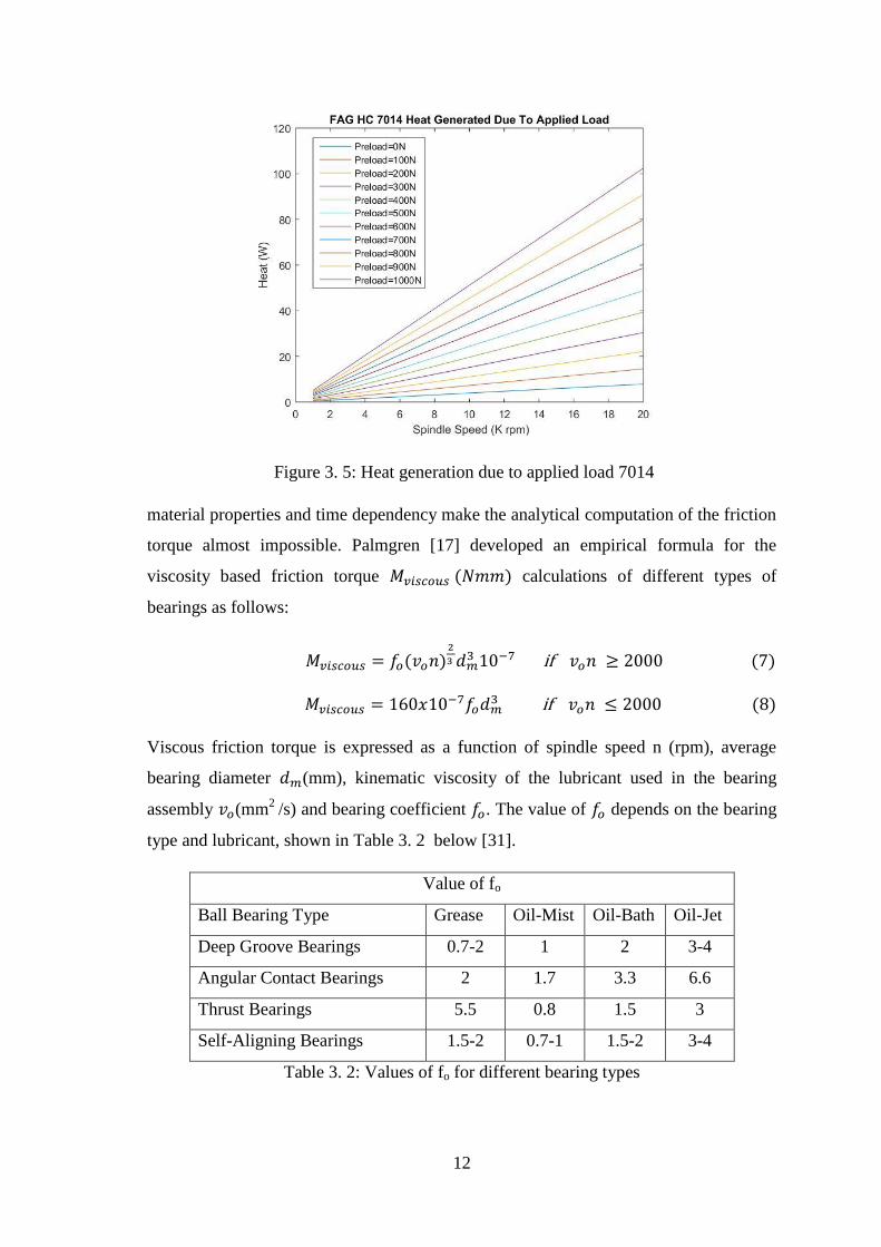
Figure 3. 5. It can be clearly seen that the heat generation is directly proportional to
preload and the spindle speed. The difference between the diameters of the bearing sets
is the only reason of the difference in the calculated heat values.
Figure 3. 4: Heat generation due to applied load 7011
3.3 Friction Torque Due to Viscosity of the Lubricant
Lubrication is vital process for increasing the fatigue lives of the mechanical joints and
continuously moving parts because of its friction reducing effect. There are different
kinds of lubrication systems and lubricants according to the bearing types and field of
application. In case of high speed ball bearings, grease lubrication is the most widely
used technique. The complexity of the bearing geometry, temperature dependent
12
Figure 3. 5: Heat generation due to applied load 7014
material properties and time dependency make the analytical computation of the friction
torque almost impossible. Palmgren [17] developed an empirical formula for the
viscosity based friction torque 𝑀𝑣𝑖𝑠𝑐𝑜𝑢𝑠 (𝑁𝑚𝑚) calculations of different types of
bearings as follows:
𝑀𝑣𝑖𝑠𝑐𝑜𝑢𝑠 = 𝑓𝑜(𝑣𝑜𝑛)2
3 𝑑𝑚3 10−7 if 𝑣𝑜𝑛 ≥ 2000 (7)
𝑀𝑣𝑖𝑠𝑐𝑜𝑢𝑠 = 160𝑥10−7𝑓𝑜𝑑𝑚3 if 𝑣𝑜𝑛 ≤ 2000 (8)
Viscous friction torque is expressed as a function of spindle speed n (rpm), average
bearing diameter 𝑑𝑚(mm), kinematic viscosity of the lubricant used in the bearing
assembly 𝑣𝑜(mm2
/s) and bearing coefficient 𝑓𝑜. The value of 𝑓𝑜 depends on the bearing
type and lubricant, shown in Table 3. 2 below [31].
Value of fo
Ball Bearing Type Grease Oil-Mist Oil-Bath Oil-Jet
Deep Groove Bearings 0.7-2 1 2 3-4
Angular Contact Bearings 2 1.7 3.3 6.6
Thrust Bearings 5.5 0.8 1.5 3
Self-Aligning Bearings 1.5-2 0.7-1 1.5-2 3-4
Table 3. 2: Values of fo for different bearing types
13
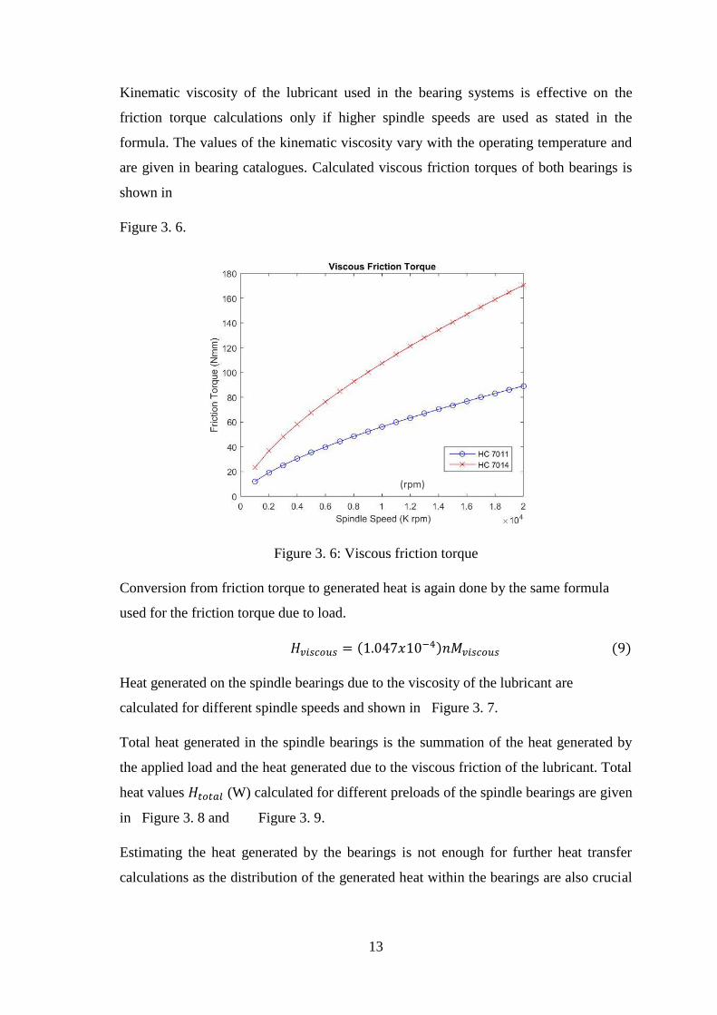
Kinematic viscosity of the lubricant used in the bearing systems is effective on the
friction torque calculations only if higher spindle speeds are used as stated in the
formula. The values of the kinematic viscosity vary with the operating temperature and
are given in bearing catalogues. Calculated viscous friction torques of both bearings is
shown in
Figure 3. 6.
Figure 3. 6: Viscous friction torque
Conversion from friction torque to generated heat is again done by the same formula
used for the friction torque due to load.
𝐻𝑣𝑖𝑠𝑐𝑜𝑢𝑠 = (1.047𝑥10−4)𝑛𝑀𝑣𝑖𝑠𝑐𝑜𝑢𝑠 (9)
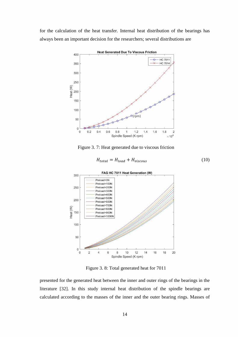
Heat generated on the spindle bearings due to the viscosity of the lubricant are
calculated for different spindle speeds and shown in Figure 3. 7.
Total heat generated in the spindle bearings is the summation of the heat generated by
the applied load and the heat generated due to the viscous friction of the lubricant. Total
heat values 𝐻𝑡𝑜𝑡𝑎𝑙 (W) calculated for different preloads of the spindle bearings are given
in Figure 3. 8 and Figure 3. 9.
Estimating the heat generated by the bearings is not enough for further heat transfer
calculations as the distribution of the generated heat within the bearings are also crucial
(rpm)
14
for the calculation of the heat transfer. Internal heat distribution of the bearings has
always been an important decision for the researchers; several distributions are
Figure 3. 7: Heat generated due to viscous friction
𝐻𝑡𝑜𝑡𝑎𝑙 = 𝐻𝑙𝑜𝑎𝑑 + 𝐻𝑣𝑖𝑠𝑐𝑜𝑢𝑠 (10)
Figure 3. 8: Total generated heat for 7011
presented for the generated heat between the inner and outer rings of the bearings in the
literature [32]. In this study internal heat distribution of the spindle bearings are
calculated according to the masses of the inner and the outer bearing rings. Masses of
(rpm)
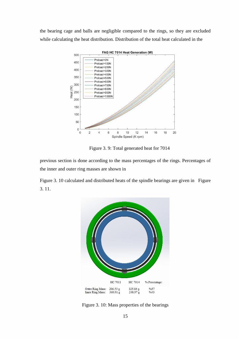
15
the bearing cage and balls are negligible compared to the rings, so they are excluded
while calculating the heat distribution. Distribution of the total heat calculated in the
Figure 3. 9: Total generated heat for 7014
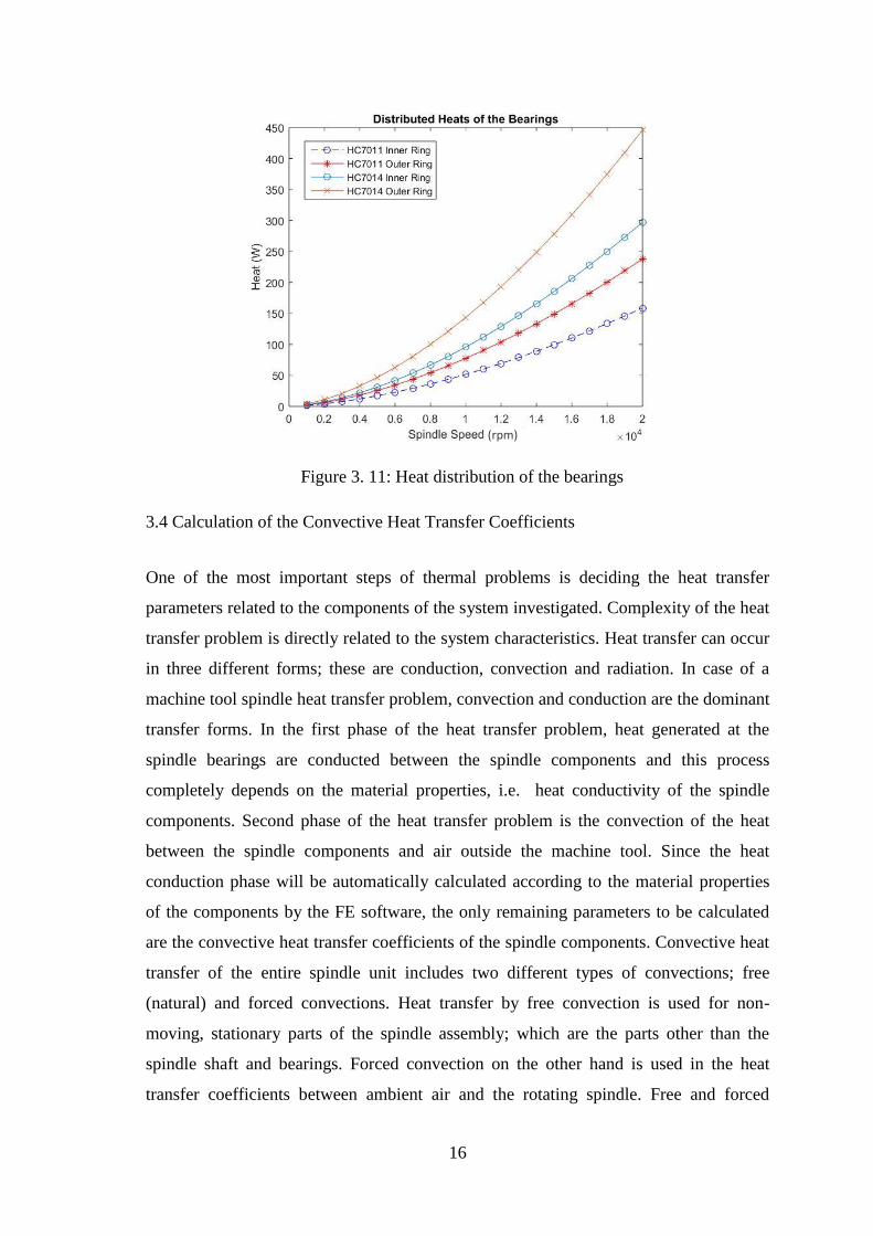
previous section is done according to the mass percentages of the rings. Percentages of
the inner and outer ring masses are shown in
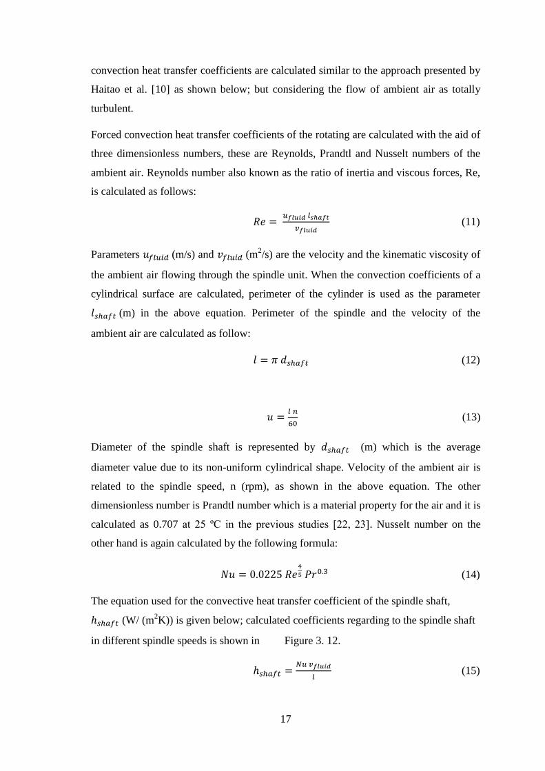
Figure 3. 10 calculated and distributed heats of the spindle bearings are given in Figure
3. 11.
Figure 3. 10: Mass properties of the bearings
16
Figure 3. 11: Heat distribution of the bearings
3.4 Calculation of the Convective Heat Transfer Coefficients
One of the most important steps of thermal problems is deciding the heat transfer
parameters related to the components of the system investigated. Complexity of the heat
transfer problem is directly related to the system characteristics. Heat transfer can occur
in three different forms; these are conduction, convection and radiation. In case of a
machine tool spindle heat transfer problem, convection and conduction are the dominant
transfer forms. In the first phase of the heat transfer problem, heat generated at the
spindle bearings are conducted between the spindle components and this process
completely depends on the material properties, i.e. heat conductivity of the spindle
components. Second phase of the heat transfer problem is the convection of the heat
between the spindle components and air outside the machine tool. Since the heat
conduction phase will be automatically calculated according to the material properties
of the components by the FE software, the only remaining parameters to be calculated
are the convective heat transfer coefficients of the spindle components. Convective heat
transfer of the entire spindle unit includes two different types of convections; free
(natural) and forced convections. Heat transfer by free convection is used for non-
moving, stationary parts of the spindle assembly; which are the parts other than the
spindle shaft and bearings. Forced convection on the other hand is used in the heat
transfer coefficients between ambient air and the rotating spindle. Free and forced
(rpm)
17
convection heat transfer coefficients are calculated similar to the approach presented by
Haitao et al. [10] as shown below; but considering the flow of ambient air as totally
turbulent.
Forced convection heat transfer coefficients of the rotating are calculated with the aid of
three dimensionless numbers, these are Reynolds, Prandtl and Nusselt numbers of the
ambient air. Reynolds number also known as the ratio of inertia and viscous forces, Re,
is calculated as follows:
𝑅𝑒 = 𝑢𝑓𝑙𝑢𝑖𝑑 𝑙𝑠ℎ𝑎𝑓𝑡
𝑣𝑓𝑙𝑢𝑖𝑑 (11)
Parameters 𝑢𝑓𝑙𝑢𝑖𝑑 (m/s) and 𝑣𝑓𝑙𝑢𝑖𝑑 (m2/s) are the velocity and the kinematic viscosity of
the ambient air flowing through the spindle unit. When the convection coefficients of a
cylindrical surface are calculated, perimeter of the cylinder is used as the parameter
𝑙𝑠ℎ𝑎𝑓𝑡 (m) in the above equation. Perimeter of the spindle and the velocity of the
ambient air are calculated as follow:
𝑙 = 𝜋 𝑑𝑠ℎ𝑎𝑓𝑡 (12)
𝑢 =𝑙 𝑛
60 (13)
Diameter of the spindle shaft is represented by 𝑑𝑠ℎ𝑎𝑓𝑡 (m) which is the average
diameter value due to its non-uniform cylindrical shape. Velocity of the ambient air is
related to the spindle speed, n (rpm), as shown in the above equation. The other
dimensionless number is Prandtl number which is a material property for the air and it is
calculated as 0.707 at 25 ºC in the previous studies [22, 23]. Nusselt number on the
other hand is again calculated by the following formula:
𝑁𝑢 = 0.0225 𝑅𝑒4
5 𝑃𝑟0.3 (14)
The equation used for the convective heat transfer coefficient of the spindle shaft,
ℎ𝑠ℎ𝑎𝑓𝑡 (W/ (m2K)) is given below; calculated coefficients regarding to the spindle shaft
in different spindle speeds is shown in Figure 3. 12.
ℎ𝑠ℎ𝑎𝑓𝑡 =𝑁𝑢 𝑣𝑓𝑙𝑢𝑖𝑑
𝑙 (15)

18
Figure 3. 12: Convective heat transfer coefficients of the spindle shaft
Free convection coefficient for the stationary (non-rotating) spindle components is
taken from the literature as 9.7 (W/ (m2K)) [10, 22, 23]. This value of the convection
coefficient is calculated according to the free convection along a flat plane phenomenon
[33].
3.5 Summary
In this chapter, empirical heat generation model used in this study is explained in detail.
Heat generated by the bearing sets of the investigated spindle unit are calculated by
using the explained model. Effect of bearing preload is shown by using different
preload values for the heat calculations. Calculated heat is distributed among the inner
and outer rings of the bearings with respect to their masses. Convective heat transfer
coefficients are calculated for stationary and rotating parts separately. At the end of this
chapter, all of the heat sources (bearing heats) and cooling parameters (convective heat
transfer coefficients) are calculated for the FEM model, which is going to use these
values as inputs for calculating the overall temperature distributions.
19
CHAPTER 4
4. FINITE ELEMENTS MODEL OF THE SPINDLE UNIT
4.1 Introduction
In this chapter Finite Elements (FE) model developed for the investigated machine tool
spindle unit is presented. 3D models of the spindle components and the assembly of the
entire spindle unit is explained with figures. There are several modeling blocks used to
represent the different stages of the thermal deformation of the machine tool spindle;
these are cooling system, temperature distribution and static deformation blocks. Details
of these simulation steps and the overall modeling strategy are explained respectively.
Boundary conditions of different FE model blocks, geometrical and theoretical
assumptions made in order to simplify both solid model and the thermal problem,
considering the solution time and accuracy constraints, are discussed. Effects of the
cooling system parameters, spindle speed and running time of the machine tool spindle
are investigated by comparing different simulation results. Example simulation results
and screenshots are provided for better visualization of the process.
4.2 Cooling System Model (CFX-CFD)
Machine tool spindles are complex electro-mechanical systems which consume high
amount of energy while generating the rotation needed for cutting tools. In the previous
chapter, reasons for heat generation and temperature rise in spindle units are explained
with their effect on the resultant positioning errors. Advanced cooling systems are
designed to decrease the effects of generated heat and temperature rise for improving
the dimensional accuracies of the machined parts. There are water, air and hybrid
cooling systems, which include both water and air together as cooling fluids. The main
20
objective of these systems is to create heat sinks near the major heat sources of the
spindle unit, such as ball bearings and spindle motor. By removing the generated heat,
thermally stable environment can be achieved and the thermal elongations can be
eliminated.
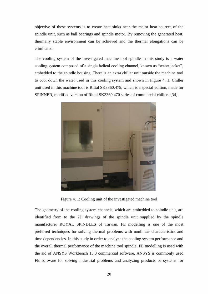
The cooling system of the investigated machine tool spindle in this study is a water
cooling system composed of a single helical cooling channel, known as “water jacket”,
embedded to the spindle housing. There is an extra chiller unit outside the machine tool
to cool down the water used in this cooling system and shown in Figure 4. 1. Chiller
unit used in this machine tool is Rittal SK3360.475, which is a special edition, made for
SPINNER, modified version of Rittal SK3360.470 series of commercial chillers [34].
Figure 4. 1: Cooling unit of the investigated machine tool
The geometry of the cooling system channels, which are embedded to spindle unit, are
identified from to the 2D drawings of the spindle unit supplied by the spindle
manufacturer ROYAL SPINDLES of Taiwan. FE modelling is one of the most
preferred techniques for solving thermal problems with nonlinear characteristics and
time dependencies. In this study in order to analyze the cooling system performance and
the overall thermal performance of the machine tool spindle, FE modelling is used with
the aid of ANSYS Workbench 15.0 commercial software. ANSYS is commonly used
FE software for solving industrial problems and analyzing products or systems for
21
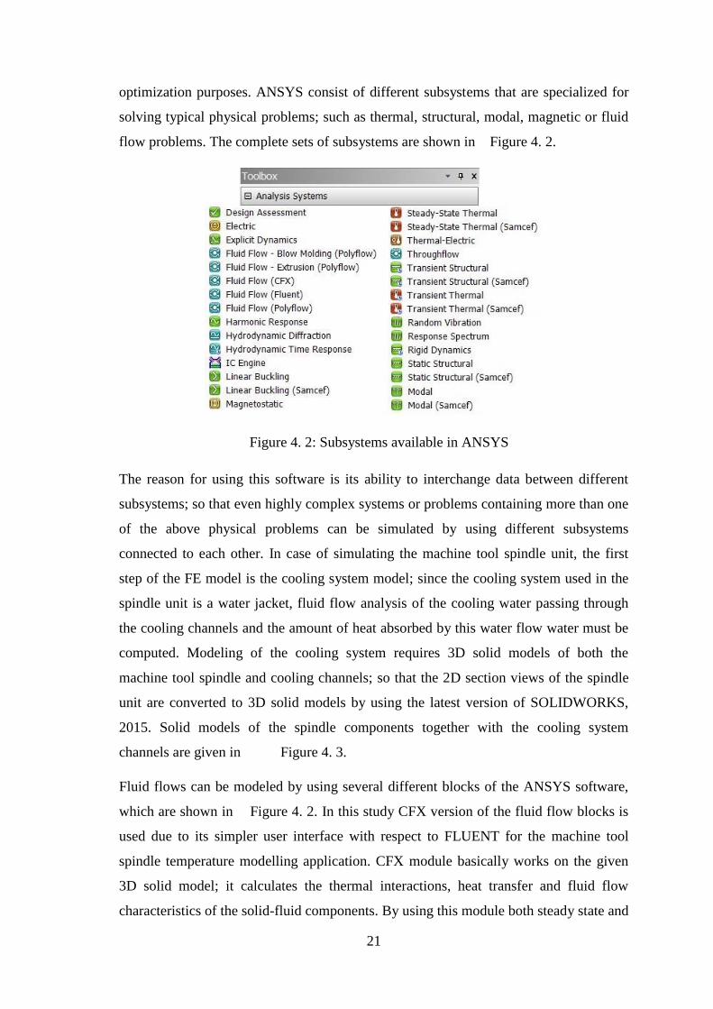
optimization purposes. ANSYS consist of different subsystems that are specialized for
solving typical physical problems; such as thermal, structural, modal, magnetic or fluid
flow problems. The complete sets of subsystems are shown in Figure 4. 2.
Figure 4. 2: Subsystems available in ANSYS
The reason for using this software is its ability to interchange data between different
subsystems; so that even highly complex systems or problems containing more than one
of the above physical problems can be simulated by using different subsystems
connected to each other. In case of simulating the machine tool spindle unit, the first
step of the FE model is the cooling system model; since the cooling system used in the
spindle unit is a water jacket, fluid flow analysis of the cooling water passing through
the cooling channels and the amount of heat absorbed by this water flow water must be
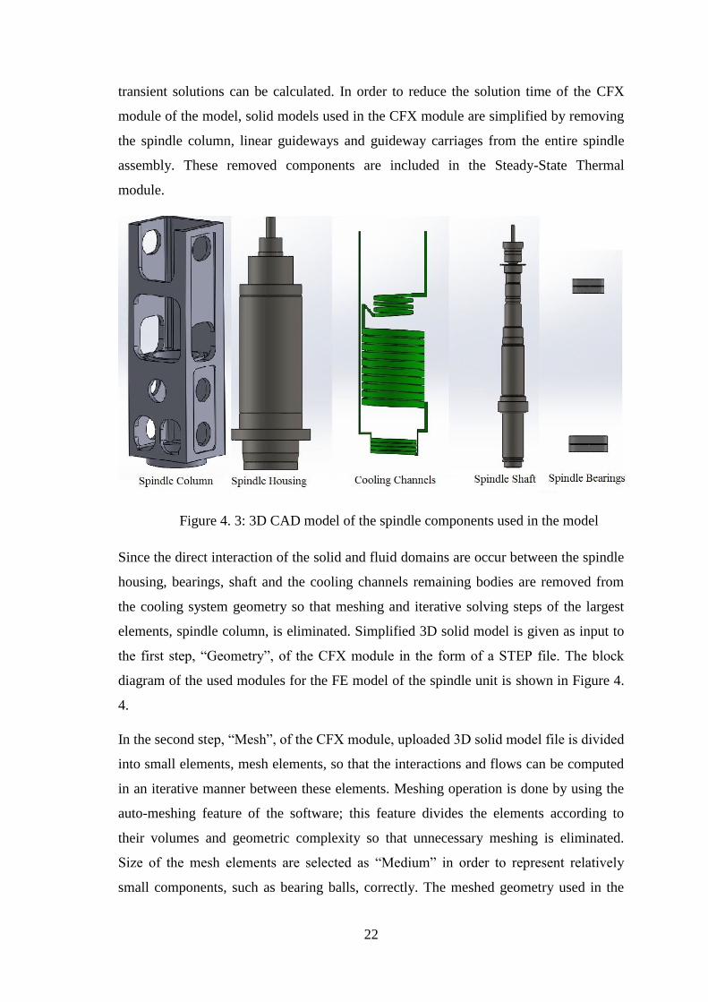
computed. Modeling of the cooling system requires 3D solid models of both the
machine tool spindle and cooling channels; so that the 2D section views of the spindle
unit are converted to 3D solid models by using the latest version of SOLIDWORKS,
2015. Solid models of the spindle components together with the cooling system
channels are given in Figure 4. 3.
Fluid flows can be modeled by using several different blocks of the ANSYS software,
which are shown in Figure 4. 2. In this study CFX version of the fluid flow blocks is
used due to its simpler user interface with respect to FLUENT for the machine tool
spindle temperature modelling application. CFX module basically works on the given
3D solid model; it calculates the thermal interactions, heat transfer and fluid flow
characteristics of the solid-fluid components. By using this module both steady state and
22
transient solutions can be calculated. In order to reduce the solution time of the CFX
module of the model, solid models used in the CFX module are simplified by removing
the spindle column, linear guideways and guideway carriages from the entire spindle
assembly. These removed components are included in the Steady-State Thermal
module.
Figure 4. 3: 3D CAD model of the spindle components used in the model
Since the direct interaction of the solid and fluid domains are occur between the spindle
housing, bearings, shaft and the cooling channels remaining bodies are removed from
the cooling system geometry so that meshing and iterative solving steps of the largest
elements, spindle column, is eliminated. Simplified 3D solid model is given as input to
the first step, “Geometry”, of the CFX module in the form of a STEP file. The block
diagram of the used modules for the FE model of the spindle unit is shown in Figure 4.
4.
In the second step, “Mesh”, of the CFX module, uploaded 3D solid model file is divided
into small elements, mesh elements, so that the interactions and flows can be computed
in an iterative manner between these elements. Meshing operation is done by using the
auto-meshing feature of the software; this feature divides the elements according to
their volumes and geometric complexity so that unnecessary meshing is eliminated.
Size of the mesh elements are selected as “Medium” in order to represent relatively
small components, such as bearing balls, correctly. The meshed geometry used in the
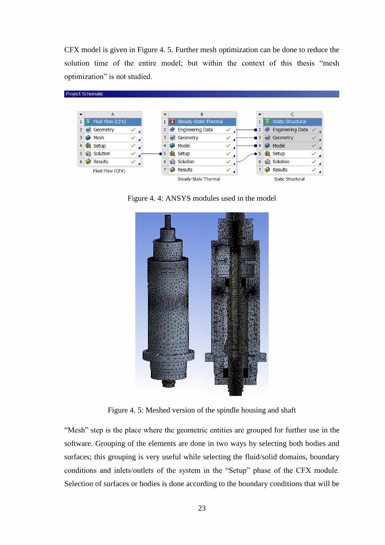
23
CFX model is given in Figure 4. 5. Further mesh optimization can be done to reduce the
solution time of the entire model; but within the context of this thesis “mesh
optimization” is not studied.
Figure 4. 4: ANSYS modules used in the model
Figure 4. 5: Meshed version of the spindle housing and shaft
“Mesh” step is the place where the geometric entities are grouped for further use in the
software. Grouping of the elements are done in two ways by selecting both bodies and
surfaces; this grouping is very useful while selecting the fluid/solid domains, boundary
conditions and inlets/outlets of the system in the “Setup” phase of the CFX module.
Selection of surfaces or bodies is done according to the boundary conditions that will be
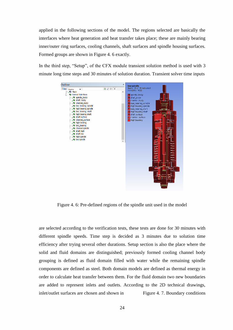
24
applied in the following sections of the model. The regions selected are basically the
interfaces where heat generation and heat transfer takes place; these are mainly bearing
inner/outer ring surfaces, cooling channels, shaft surfaces and spindle housing surfaces.
Formed groups are shown in Figure 4. 6 exactly.
In the third step, “Setup”, of the CFX module transient solution method is used with 3
minute long time steps and 30 minutes of solution duration. Transient solver time inputs
Figure 4. 6: Pre-defined regions of the spindle unit used in the model
are selected according to the verification tests, these tests are done for 30 minutes with
different spindle speeds. Time step is decided as 3 minutes due to solution time
efficiency after trying several other durations. Setup section is also the place where the
solid and fluid domains are distinguished; previously formed cooling channel body
grouping is defined as fluid domain filled with water while the remaining spindle
components are defined as steel. Both domain models are defined as thermal energy in
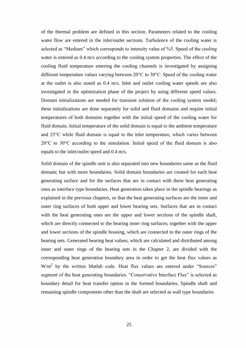
order to calculate heat transfer between them. For the fluid domain two new boundaries
are added to represent inlets and outlets. According to the 2D technical drawings,
inlet/outlet surfaces are chosen and shown in Figure 4. 7. Boundary conditions
25
of the thermal problem are defined in this section. Parameters related to the cooling
water flow are entered in the inlet/outlet sections. Turbulence of the cooling water is
selected as “Medium” which corresponds to intensity value of %5. Speed of the cooling
water is entered as 0.4 m/s according to the cooling system properties. The effect of the
cooling fluid temperature entering the cooling channels is investigated by assigning
different temperature values varying between 20°C to 30°C. Speed of the cooling water
at the outlet is also stated as 0.4 m/s. Inlet and outlet cooling water speeds are also
investigated in the optimization phase of the project by using different speed values.
Domain initializations are needed for transient solution of the cooling system model;
these initializations are done separately for solid and fluid domains and require initial
temperatures of both domains together with the initial speed of the cooling water for
fluid domain. Initial temperature of the solid domain is equal to the ambient temperature
and 25°C while fluid domain is equal to the inlet temperature, which varies between
20°C to 30°C according to the simulation. Initial speed of the fluid domain is also
equals to the inlet/outlet speed and 0.4 m/s.
Solid domain of the spindle unit is also separated into new boundaries same as the fluid
domain; but with more boundaries. Solid domain boundaries are created for each heat
generating surface and for the surfaces that are in contact with these heat generating
ones as interface type boundaries. Heat generation takes place in the spindle bearings as
explained in the previous chapters, so that the heat generating surfaces are the inner and
outer ring surfaces of both upper and lower bearing sets. Surfaces that are in contact
with the heat generating ones are the upper and lower sections of the spindle shaft,
which are directly connected to the bearing inner ring surfaces; together with the upper
and lower sections of the spindle housing, which are connected to the outer rings of the
bearing sets. Generated bearing heat values, which are calculated and distributed among
inner and outer rings of the bearing sets in the Chapter 2, are divided with the
corresponding heat generation boundary area in order to get the heat flux values as
W/m2 by the written Matlab code. Heat flux values are entered under “Sources”
segment of the heat generating boundaries. “Conservative Interface Flux” is selected as
boundary detail for heat transfer option in the formed boundaries. Spindle shaft and
remaining spindle components other than the shaft are selected as wall type boundaries
26
Figure 4. 7: Outline of the spindle CAD model used in CFX module
because of the convective heat transfer taking place on their surface. Convective heat
transfer coefficients calculated in the Chapter 2 are used in here to represent the
convective cooling. Convective heat transfer of the spindle shaft is calculated according
to the spindle speed as explained in the previous chapter and entered to the “Boundary
Detail” segment. Constant convective heat transfer coefficient of 9.7 (W/ (m2K)) is used
for the remaining spindle components again as explained in the previous chapter.
Setup step is finalized by adding the necessary interfaces to the model under the
“Interfaces” tab of the model tree. Interfaces are basically the boundaries created in the
solid domain as heat generating surfaces and other surfaces that are connected to them.
All interfaces are created with heat transfer option enabled. In the interfaces tab
boundaries which heat transfer takes place are selected, interfaces are divided into two
as solid- solid and solid-fluid interfaces. Solid-fluid interface takes place between the
spindle housing and the cooling channels while solid-solid interfaces are as follows:

27
- Upper bearing set inner ring surface – portion of the spindle shaft that is in
contact with upper bearings
- Upper bearing set outer ring surface – portion of the spindle housing that is in
contact with upper bearings
- Lower bearing set inner ring – portion of the spindle shaft that is in contact with
lower bearings
- Lower bearing set outer ring – portion of the spindle housing that is in contact
with lower bearings
- Upper and lower bearing inner rings, outer rings and bearing balls.
Model tree of the explained process, domains, boundaries and interfaces created are
shown in Figure 4. 8 below.
Figure 4. 8: Model tree of the CFX module

28
Last two steps of the CFX module are “Solution” and “Results”, which are used for
monitoring applications. Solver iterations and the calculated values of the model error
together with the convergence graph can be monitored by the solution step. Results on
the other hand are used for visualization of the calculated results related to the solved
model. In case of the spindle unit thermal problem, final temperatures of the model
components are investigated by the graphical tools provided in the results section.
Physical properties such as temperature and velocity of the cooling water, spindle
housing and shaft are plotted in this section.
4.3 Thermal Model
FE model developed for the Spinner U-1520 machine tool spindle unit uses “Steady-
State Thermal” analysis module to calculate temperatures of the spindle components
that are not included in the CFX module geometry due to the solution time optimization
purposes. Thermal module is generally used for the heat transfer calculations within the
given geometries. The components that are excluded from the CFX module geometry
are the spindle column, linear guideways and the guideway carriages, shown in Figure
4. 9 below.
Figure 4. 9: 3D CAD models of the overall spindle unit used in the thermal module
29
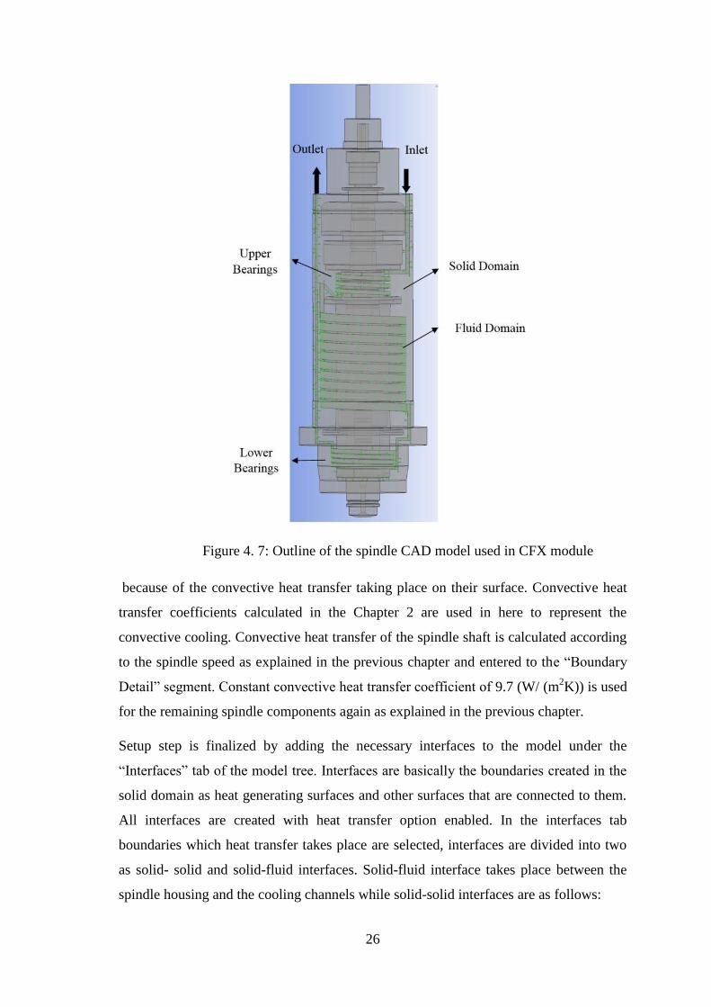
Thermal module is connected directly to the solution step of the CFX module in order to
transfer data from CFX module. The data transferred in the model is the temperatures of
the spindle unit components which are calculated at the CFX module. This temperature
data is used by thermal module to calculate the individual temperature distributions of
the newly added components. The transferred data includes the individual temperatures
of the spindle housing, cooling channels, and spindle shaft, upper and lower bearings.
Temperatures transferred from the CFX module as “Imported Loads” are shown in
Figure 4. 10.
Figure 4. 10: Imported Loads
4.4 Static Structural Model
The overall aim of the developed FE model is to predict the thermal elongations of the
machine tool spindle. However, the first two modules explained above are both used to
find the temperature distribution of the entire spindle unit by considering the effects of
the cooling system. Since the investigated elongations are due to the thermal state of the
machine tool components, calculation of the heat distribution is crucial. The next step
after calculating the temperature distribution is to determine the elongations caused by
the temperature distribution. Static Structural module used at the end of the project
scheme as the third module calculates the thermal elongations of the spindle unit
components. Physical boundary conditions, such as gravitational force acting on the
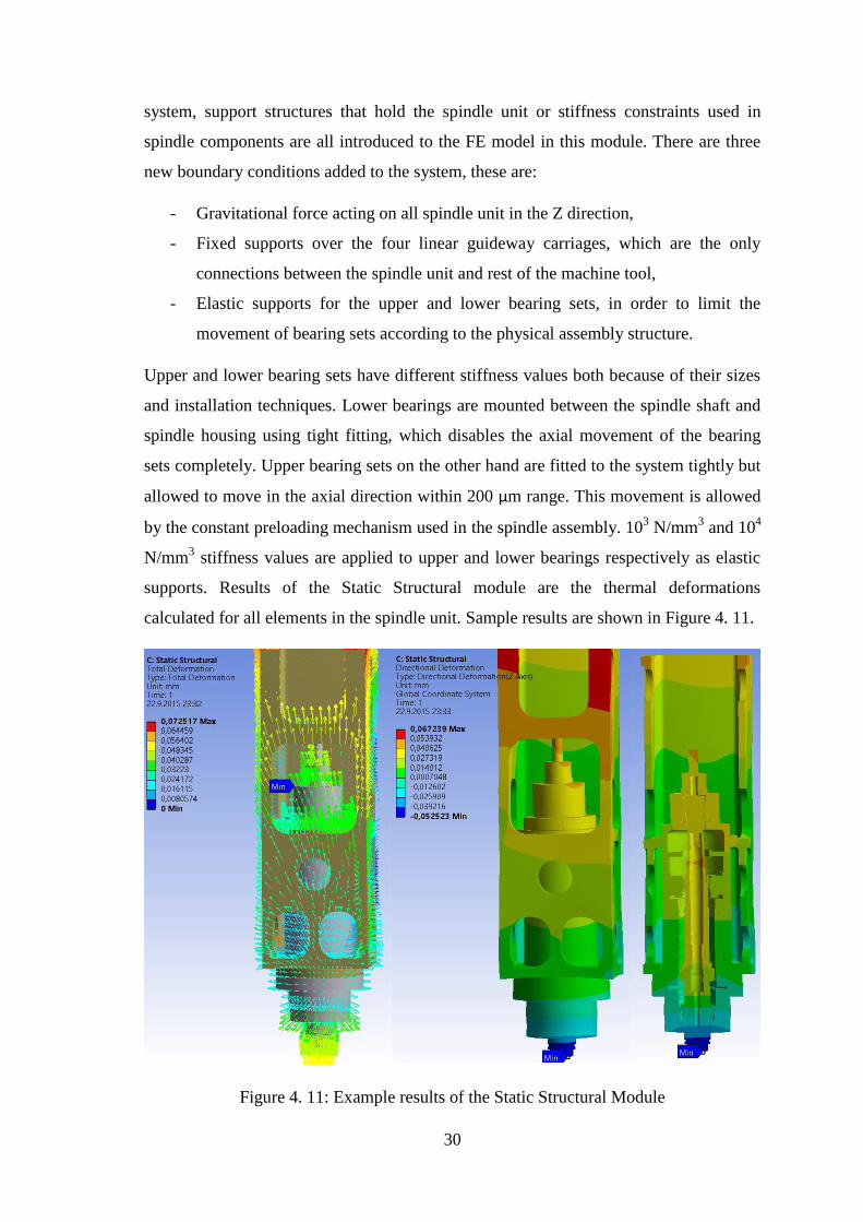
30
system, support structures that hold the spindle unit or stiffness constraints used in
spindle components are all introduced to the FE model in this module. There are three
new boundary conditions added to the system, these are:
- Gravitational force acting on all spindle unit in the Z direction,
- Fixed supports over the four linear guideway carriages, which are the only
connections between the spindle unit and rest of the machine tool,
- Elastic supports for the upper and lower bearing sets, in order to limit the
movement of bearing sets according to the physical assembly structure.
Upper and lower bearing sets have different stiffness values both because of their sizes
and installation techniques. Lower bearings are mounted between the spindle shaft and
spindle housing using tight fitting, which disables the axial movement of the bearing
sets completely. Upper bearing sets on the other hand are fitted to the system tightly but
allowed to move in the axial direction within 200 µm range. This movement is allowed
by the constant preloading mechanism used in the spindle assembly. 103 N/mm
3 and 10
4
N/mm3 stiffness values are applied to upper and lower bearings respectively as elastic
supports. Results of the Static Structural module are the thermal deformations
calculated for all elements in the spindle unit. Sample results are shown in Figure 4. 11.
Figure 4. 11: Example results of the Static Structural Module
31
4.5 Model Simulations
The FEM model is used to simulate several tests for comparison of the results to check
the prediction accuracy. The tests that are simulated with the model are the short
duration tests of 30 minutes and 5000-10000-15000-20000 rpms of spindle speeds.
Detailed results of the FEM model simulations using these 4 different test parameters
are given below.
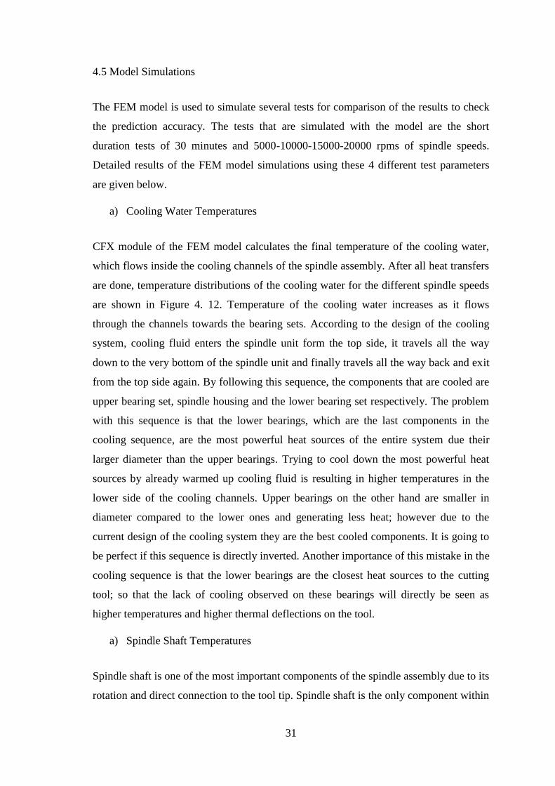
a) Cooling Water Temperatures
CFX module of the FEM model calculates the final temperature of the cooling water,
which flows inside the cooling channels of the spindle assembly. After all heat transfers
are done, temperature distributions of the cooling water for the different spindle speeds
are shown in Figure 4. 12. Temperature of the cooling water increases as it flows
through the channels towards the bearing sets. According to the design of the cooling
system, cooling fluid enters the spindle unit form the top side, it travels all the way
down to the very bottom of the spindle unit and finally travels all the way back and exit
from the top side again. By following this sequence, the components that are cooled are
upper bearing set, spindle housing and the lower bearing set respectively. The problem
with this sequence is that the lower bearings, which are the last components in the
cooling sequence, are the most powerful heat sources of the entire system due their
larger diameter than the upper bearings. Trying to cool down the most powerful heat
sources by already warmed up cooling fluid is resulting in higher temperatures in the
lower side of the cooling channels. Upper bearings on the other hand are smaller in
diameter compared to the lower ones and generating less heat; however due to the
current design of the cooling system they are the best cooled components. It is going to
be perfect if this sequence is directly inverted. Another importance of this mistake in the
cooling sequence is that the lower bearings are the closest heat sources to the cutting
tool; so that the lack of cooling observed on these bearings will directly be seen as
higher temperatures and higher thermal deflections on the tool.
a) Spindle Shaft Temperatures
Spindle shaft is one of the most important components of the spindle assembly due to its
rotation and direct connection to the tool tip. Spindle shaft is the only component within
32
the spindle assembly which does not have built-in cooling channels. Cooling of the
spindle shaft is achieved by the bearings which are the only structures that connect
spindle shaft to the rest of the spindle assembly. The lack of cooling system is combined
with the direct connection to the main heat sources of the system, bearings, and making
the spindle shaft the hottest component of the entire assembly. Locations around the
bearing inner rings are expected to be the hottest regions on the shaft. Spindle shaft
temperatures calculated for different spindle speeds are given in Figure 4. 13 below. As
in the cooling water simulations, shaft temperature increases with the increasing spindle
speed and bearing locations on the shaft are the hottest regions as expected.
a) Spindle Surface Temperatures
Temperatures of the entire spindle surface are also calculated by the CFX module
within the FEM model. Spindle outer surface is cooler compared to other parts of the
assembly because of its distance to the main heat sources and the convectional heat
transfer taking place between the outer surface of the spindle and the air outside.
Calculated temperatures of the spindle surface are given in Figure 4. 13. These figures
show the spindle inner surface which is in contact with bearing outer rings. High
temperature values seen at the legend belong to the bearing rings. The effect of the
spindle speed is again obvious on the temperatures which increase with the spindle
speed.
Temperature prediction results for four different tests are compared on a single graph
given in Figure 4. 15, showing the effect of spindle speed. Cooling water temperatures
are lower than the shaft and spindle temperatures according to the graph. The reason for
shaft and spindle surface temperatures being so close to each other is their direct
connection to the spindle bearings, which are the only heat sources of the spindle
system. Outer bearing rings are connected to the spindle housing while the inner rings
are attached to the shaft. As explained in the previous chapter, outer rings of the bearing
sets receive %60 of the total generated heat and the small temperature difference
between the shaft and spindle surface is due to this partitioning of the heat between the
bearing rings.
33
Figure 4. 12: Temperature of the cooling fluids within the cooling channels for different
spindle speeds
34
Figure 4. 13: Calculated temperature distributions of the spindle shaft for different
spindle speeds
35
Figure 4. 14: Calculated temperature distributions of the spindle surfaces for different
spindle speeds
36
Figure 4. 15: Comparison of the different spindle speed simulations
b) Deflections of the Tool Tip
Predicting the thermally induced elongations of the tool tip is the main objective of the
FEM model used. According to the calculated temperature distributions, deflections of
the tool tip are calculated by the model for different spindle speeds and the results are
given in Figure 4. 16 below. The deflection of the tool tip along the Z axis increases
with the spindle speed. With the increasing spindle speed heat generated by the spindle
bearings is increases and causing higher temperature distributions over the entire
spindle components. As a result of these higher temperature distributions, tool tip
deflections are also increasing accordingly. The nonlinear relationship between the
spindle speed and tool tip elongations is given as a chart for visualization of the results
in Figure 4. 17.
4.6 Summary
In this chapter, FEM model developed for the calculating the temperature distributions
and thermal deformations are explained in detail. Modules used in the FEM model are
explained one by one including the inputs and outputs of each. 3D CAD models used in
each module are presented. Connections between the all three modules used in the FEM
0
10
20
30
40
50
60
70
80
5K rpm 10K rpm 15K rpm 20K rpm
Tem
per
atu
re (
°C)
Comparison of Simulation Results
Max Cooling Water Temp Max Spindle Shaft Temp Max Spindle Surface Temp
37
Figure 4. 16: Z-direction deflections of the tool tip for different spindle speeds
Figure 4. 17: Comparisons of the tool tip deflections for different spindle speeds
0
10
20
30
40
50
60
70
5K rpm 10K rpm 15K rpm 20K rpm
Def
lect
ion
(µ
m)
Tool Tip Deflections vs Spindle Speed

38
model are again explained by presenting the transferred information. In the last part of
the chapter, simulation results obtained by the proposed FEM model are shown for four
different spindle speeds. Two important outputs of the model are the temperature
distributions and the tool tip deflections due to the thermal affects. Simulation results
will be used for model validation in the upcoming chapters.
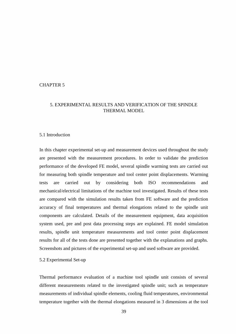
39
CHAPTER 5
5. EXPERIMENTAL RESULTS AND VERIFICATION OF THE SPINDLE
THERMAL MODEL
5.1 Introduction
In this chapter experimental set-up and measurement devices used throughout the study
are presented with the measurement procedures. In order to validate the prediction
performance of the developed FE model, several spindle warming tests are carried out
for measuring both spindle temperature and tool center point displacements. Warming
tests are carried out by considering both ISO recommendations and
mechanical/electrical limitations of the machine tool investigated. Results of these tests
are compared with the simulation results taken from FE software and the prediction
accuracy of final temperatures and thermal elongations related to the spindle unit
components are calculated. Details of the measurement equipment, data acquisition
system used, pre and post data processing steps are explained. FE model simulation
results, spindle unit temperature measurements and tool center point displacement
results for all of the tests done are presented together with the explanations and graphs.
Screenshots and pictures of the experimental set-up and used software are provided.
5.2 Experimental Set-up
Thermal performance evaluation of a machine tool spindle unit consists of several
different measurements related to the investigated spindle unit; such as temperature
measurements of individual spindle elements, cooling fluid temperatures, environmental
temperature together with the thermal elongations measured in 3 dimensions at the tool
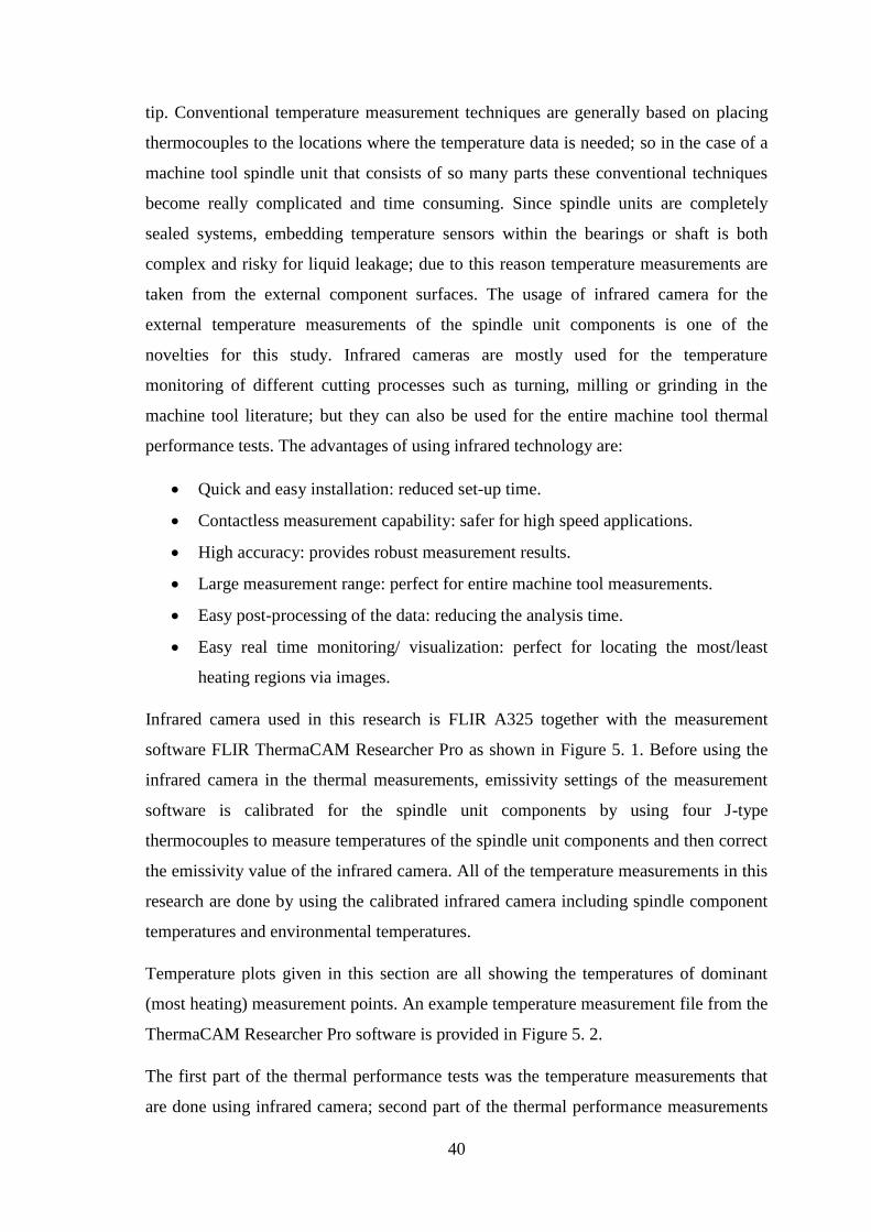
40
tip. Conventional temperature measurement techniques are generally based on placing
thermocouples to the locations where the temperature data is needed; so in the case of a
machine tool spindle unit that consists of so many parts these conventional techniques
become really complicated and time consuming. Since spindle units are completely
sealed systems, embedding temperature sensors within the bearings or shaft is both
complex and risky for liquid leakage; due to this reason temperature measurements are
taken from the external component surfaces. The usage of infrared camera for the
external temperature measurements of the spindle unit components is one of the
novelties for this study. Infrared cameras are mostly used for the temperature
monitoring of different cutting processes such as turning, milling or grinding in the
machine tool literature; but they can also be used for the entire machine tool thermal
performance tests. The advantages of using infrared technology are:
Quick and easy installation: reduced set-up time.
Contactless measurement capability: safer for high speed applications.
High accuracy: provides robust measurement results.
Large measurement range: perfect for entire machine tool measurements.
Easy post-processing of the data: reducing the analysis time.
Easy real time monitoring/ visualization: perfect for locating the most/least
heating regions via images.
Infrared camera used in this research is FLIR A325 together with the measurement
software FLIR ThermaCAM Researcher Pro as shown in Figure 5. 1. Before using the
infrared camera in the thermal measurements, emissivity settings of the measurement
software is calibrated for the spindle unit components by using four J-type
thermocouples to measure temperatures of the spindle unit components and then correct
the emissivity value of the infrared camera. All of the temperature measurements in this
research are done by using the calibrated infrared camera including spindle component
temperatures and environmental temperatures.
Temperature plots given in this section are all showing the temperatures of dominant
(most heating) measurement points. An example temperature measurement file from the
ThermaCAM Researcher Pro software is provided in Figure 5. 2.
The first part of the thermal performance tests was the temperature measurements that
are done using infrared camera; second part of the thermal performance measurements
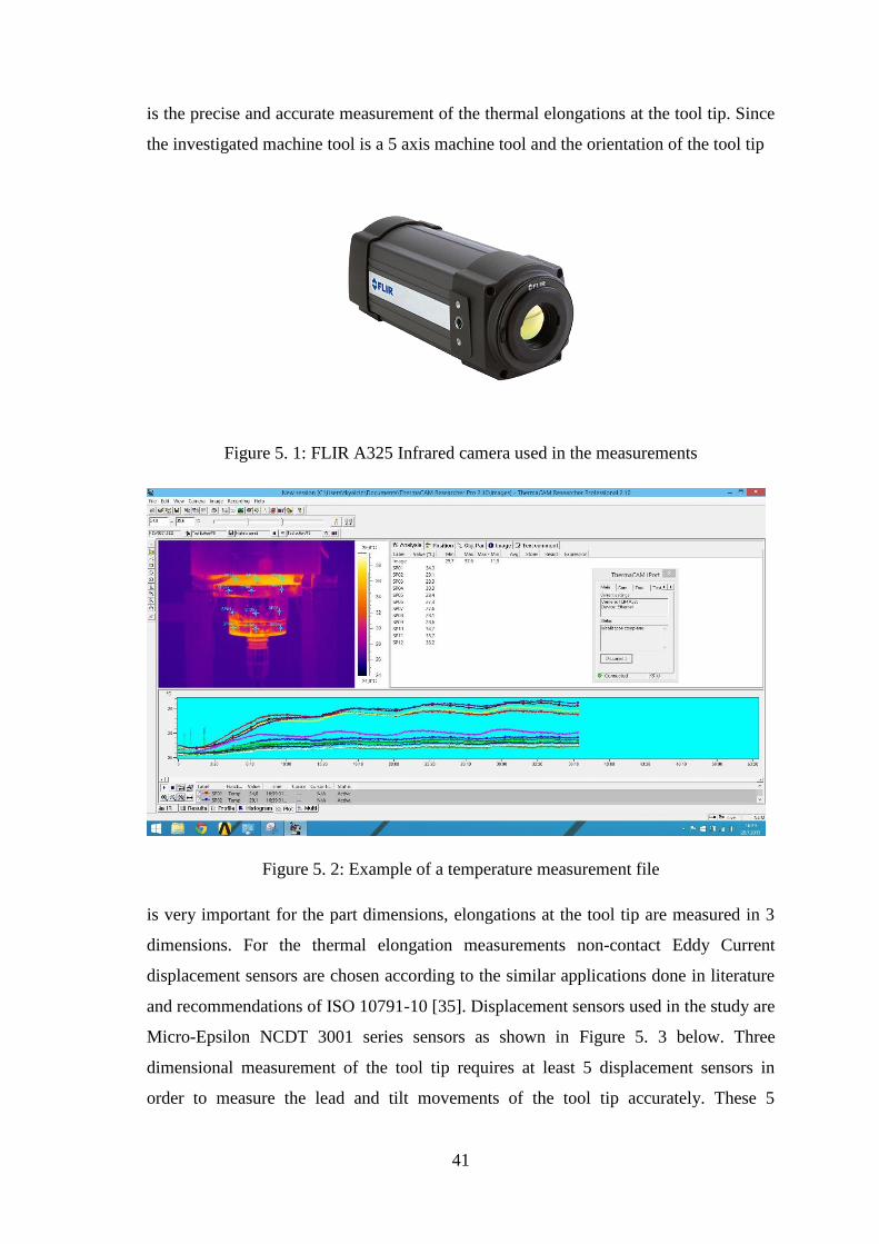
41
is the precise and accurate measurement of the thermal elongations at the tool tip. Since
the investigated machine tool is a 5 axis machine tool and the orientation of the tool tip
Figure 5. 1: FLIR A325 Infrared camera used in the measurements
Figure 5. 2: Example of a temperature measurement file
is very important for the part dimensions, elongations at the tool tip are measured in 3
dimensions. For the thermal elongation measurements non-contact Eddy Current
displacement sensors are chosen according to the similar applications done in literature
and recommendations of ISO 10791-10 [35]. Displacement sensors used in the study are
Micro-Epsilon NCDT 3001 series sensors as shown in Figure 5. 3 below. Three
dimensional measurement of the tool tip requires at least 5 displacement sensors in
order to measure the lead and tilt movements of the tool tip accurately. These 5
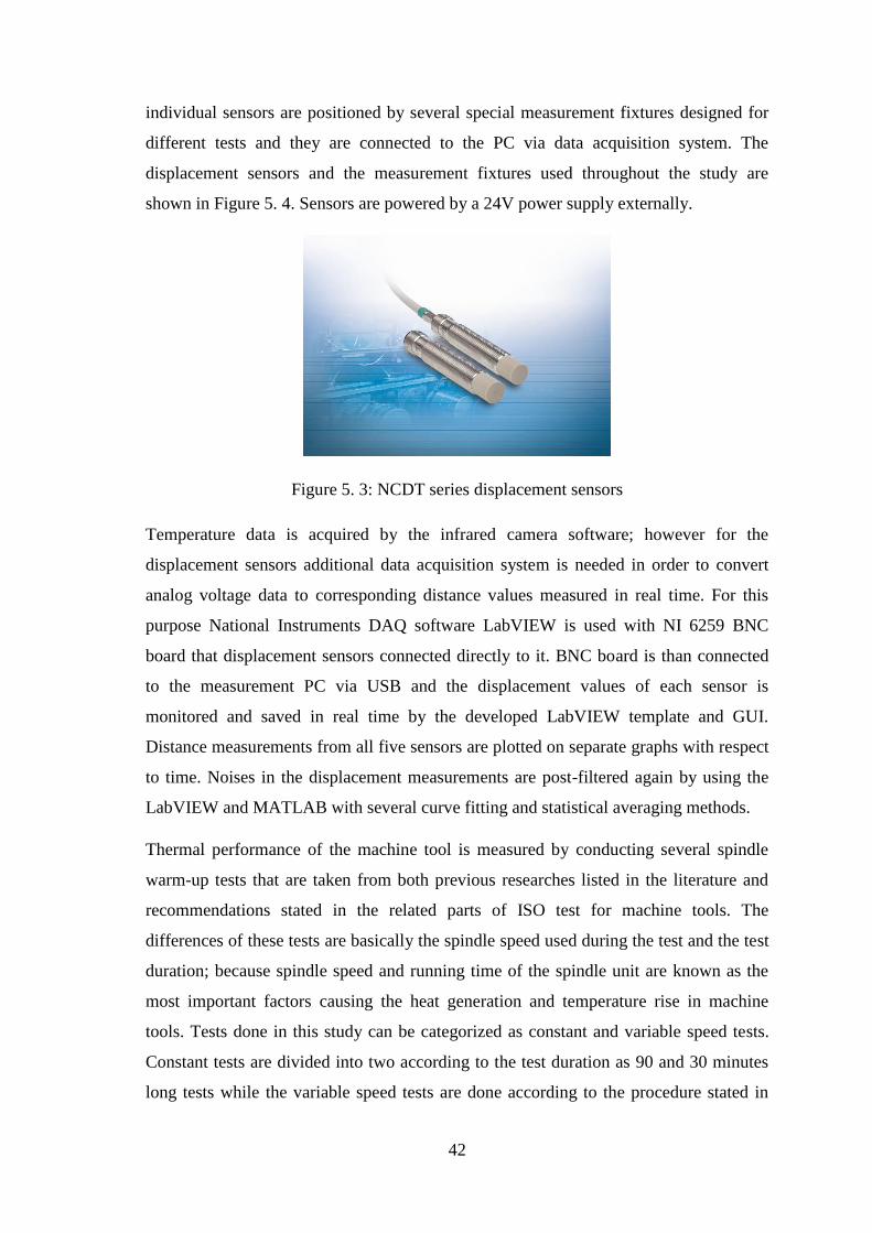
42
individual sensors are positioned by several special measurement fixtures designed for
different tests and they are connected to the PC via data acquisition system. The
displacement sensors and the measurement fixtures used throughout the study are
shown in Figure 5. 4. Sensors are powered by a 24V power supply externally.
Figure 5. 3: NCDT series displacement sensors
Temperature data is acquired by the infrared camera software; however for the
displacement sensors additional data acquisition system is needed in order to convert
analog voltage data to corresponding distance values measured in real time. For this
purpose National Instruments DAQ software LabVIEW is used with NI 6259 BNC
board that displacement sensors connected directly to it. BNC board is than connected
to the measurement PC via USB and the displacement values of each sensor is
monitored and saved in real time by the developed LabVIEW template and GUI.
Distance measurements from all five sensors are plotted on separate graphs with respect
to time. Noises in the displacement measurements are post-filtered again by using the
LabVIEW and MATLAB with several curve fitting and statistical averaging methods.
Thermal performance of the machine tool is measured by conducting several spindle
warm-up tests that are taken from both previous researches listed in the literature and
recommendations stated in the related parts of ISO test for machine tools. The
differences of these tests are basically the spindle speed used during the test and the test
duration; because spindle speed and running time of the spindle unit are known as the
most important factors causing the heat generation and temperature rise in machine
tools. Tests done in this study can be categorized as constant and variable speed tests.
Constant tests are divided into two according to the test duration as 90 and 30 minutes
long tests while the variable speed tests are done according to the procedure stated in
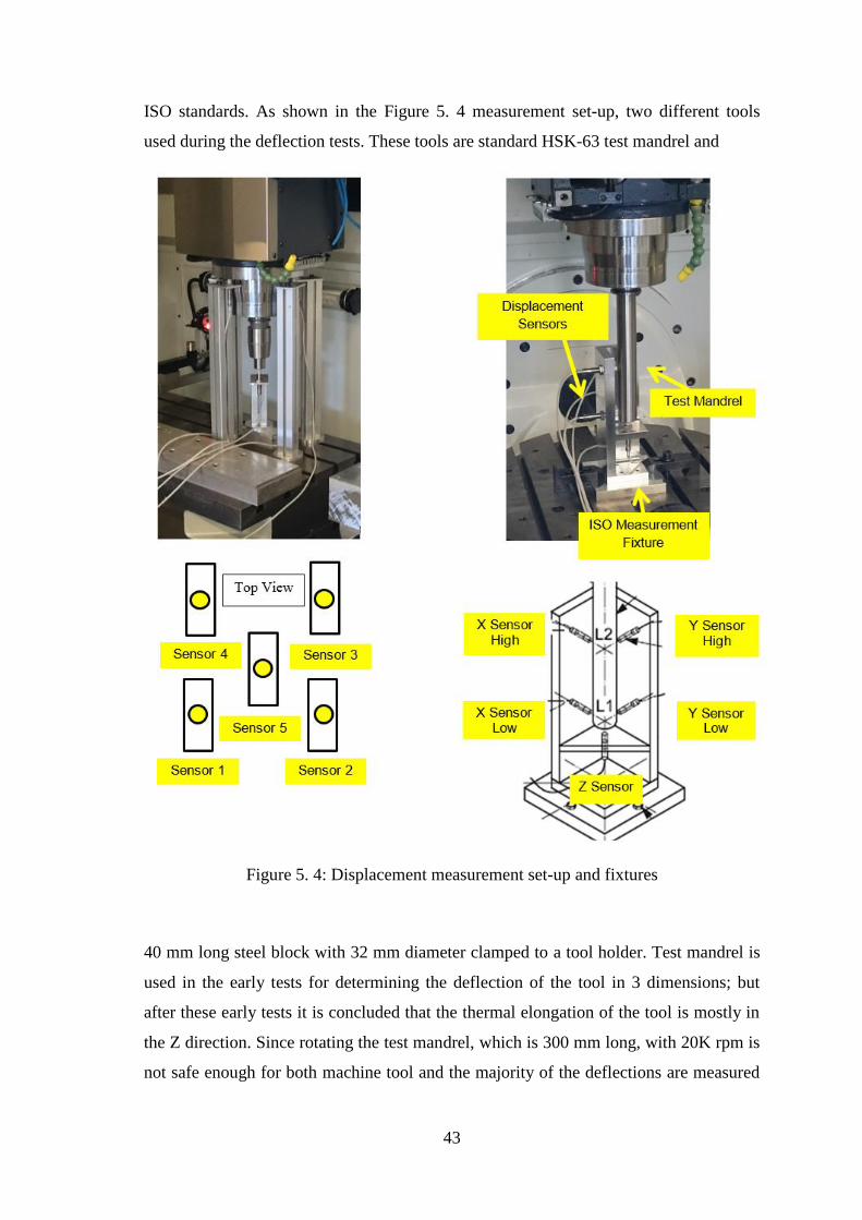
43
ISO standards. As shown in the Figure 5. 4 measurement set-up, two different tools
used during the deflection tests. These tools are standard HSK-63 test mandrel and
Figure 5. 4: Displacement measurement set-up and fixtures
40 mm long steel block with 32 mm diameter clamped to a tool holder. Test mandrel is
used in the early tests for determining the deflection of the tool in 3 dimensions; but
after these early tests it is concluded that the thermal elongation of the tool is mostly in
the Z direction. Since rotating the test mandrel, which is 300 mm long, with 20K rpm is
not safe enough for both machine tool and the majority of the deflections are measured
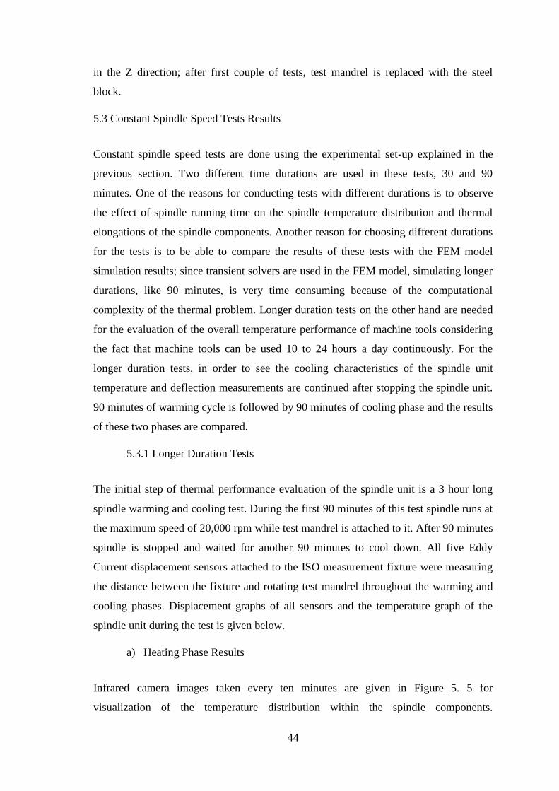
44
in the Z direction; after first couple of tests, test mandrel is replaced with the steel
block.
5.3 Constant Spindle Speed Tests Results
Constant spindle speed tests are done using the experimental set-up explained in the
previous section. Two different time durations are used in these tests, 30 and 90
minutes. One of the reasons for conducting tests with different durations is to observe
the effect of spindle running time on the spindle temperature distribution and thermal
elongations of the spindle components. Another reason for choosing different durations
for the tests is to be able to compare the results of these tests with the FEM model
simulation results; since transient solvers are used in the FEM model, simulating longer
durations, like 90 minutes, is very time consuming because of the computational
complexity of the thermal problem. Longer duration tests on the other hand are needed
for the evaluation of the overall temperature performance of machine tools considering
the fact that machine tools can be used 10 to 24 hours a day continuously. For the
longer duration tests, in order to see the cooling characteristics of the spindle unit
temperature and deflection measurements are continued after stopping the spindle unit.
90 minutes of warming cycle is followed by 90 minutes of cooling phase and the results
of these two phases are compared.
5.3.1 Longer Duration Tests
The initial step of thermal performance evaluation of the spindle unit is a 3 hour long
spindle warming and cooling test. During the first 90 minutes of this test spindle runs at
the maximum speed of 20,000 rpm while test mandrel is attached to it. After 90 minutes
spindle is stopped and waited for another 90 minutes to cool down. All five Eddy
Current displacement sensors attached to the ISO measurement fixture were measuring
the distance between the fixture and rotating test mandrel throughout the warming and
cooling phases. Displacement graphs of all sensors and the temperature graph of the
spindle unit during the test is given below.
a) Heating Phase Results
Infrared camera images taken every ten minutes are given in Figure 5. 5 for
visualization of the temperature distribution within the spindle components.
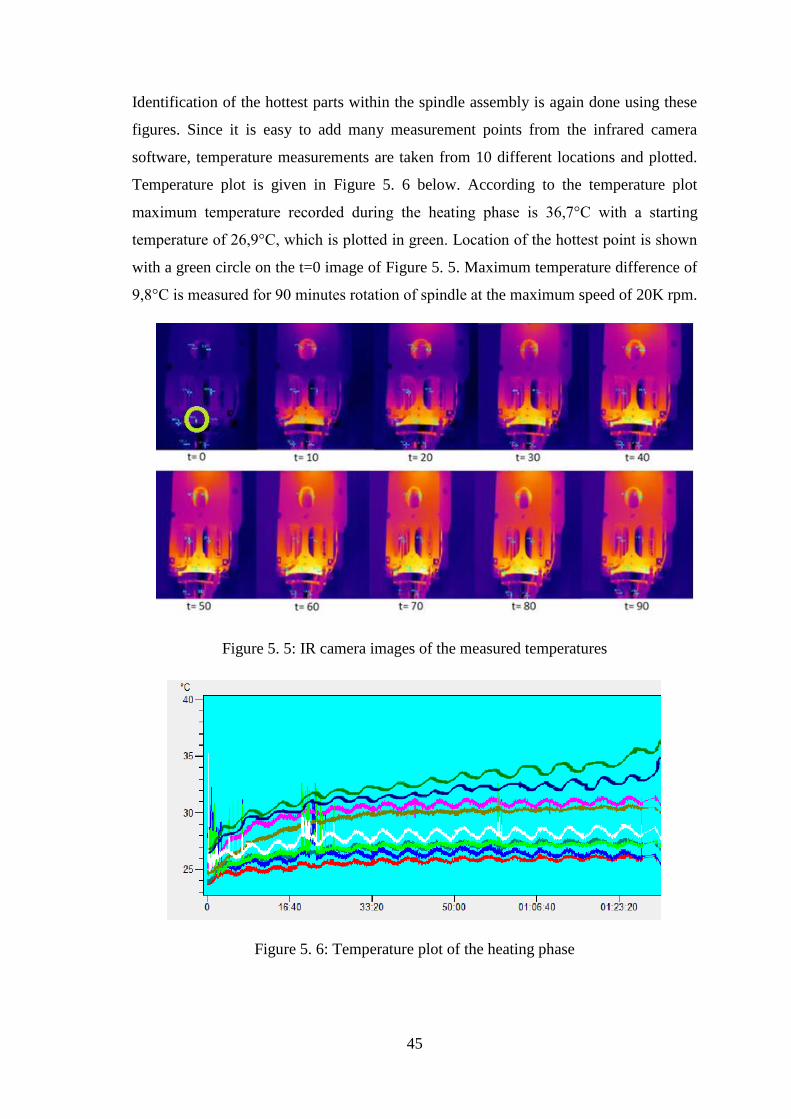
45
Identification of the hottest parts within the spindle assembly is again done using these
figures. Since it is easy to add many measurement points from the infrared camera
software, temperature measurements are taken from 10 different locations and plotted.
Temperature plot is given in Figure 5. 6 below. According to the temperature plot
maximum temperature recorded during the heating phase is 36,7°C with a starting
temperature of 26,9°C, which is plotted in green. Location of the hottest point is shown
with a green circle on the t=0 image of Figure 5. 5. Maximum temperature difference of
9,8°C is measured for 90 minutes rotation of spindle at the maximum speed of 20K rpm.
Figure 5. 5: IR camera images of the measured temperatures
Figure 5. 6: Temperature plot of the heating phase
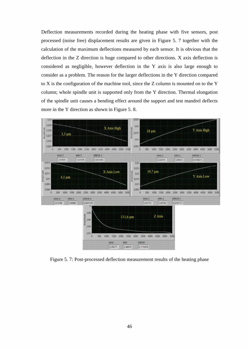
46
Deflection measurements recorded during the heating phase with five sensors, post
processed (noise free) displacement results are given in Figure 5. 7 together with the
calculation of the maximum deflections measured by each sensor. It is obvious that the
deflection in the Z direction is huge compared to other directions. X axis deflection is
considered as negligible, however deflection in the Y axis is also large enough to
consider as a problem. The reason for the larger deflections in the Y direction compared
to X is the configuration of the machine tool, since the Z column is mounted on to the Y
column; whole spindle unit is supported only from the Y direction. Thermal elongation
of the spindle unit causes a bending effect around the support and test mandrel deflects
more in the Y direction as shown in Figure 5. 8.
Figure 5. 7: Post-processed deflection measurement results of the heating phase
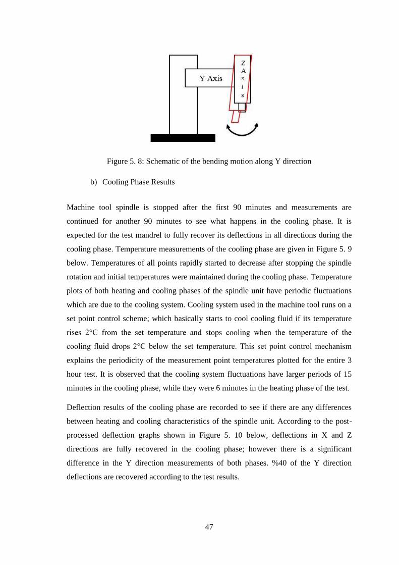
47
Figure 5. 8: Schematic of the bending motion along Y direction
b) Cooling Phase Results
Machine tool spindle is stopped after the first 90 minutes and measurements are
continued for another 90 minutes to see what happens in the cooling phase. It is
expected for the test mandrel to fully recover its deflections in all directions during the
cooling phase. Temperature measurements of the cooling phase are given in Figure 5. 9
below. Temperatures of all points rapidly started to decrease after stopping the spindle
rotation and initial temperatures were maintained during the cooling phase. Temperature
plots of both heating and cooling phases of the spindle unit have periodic fluctuations
which are due to the cooling system. Cooling system used in the machine tool runs on a
set point control scheme; which basically starts to cool cooling fluid if its temperature
rises 2°C from the set temperature and stops cooling when the temperature of the
cooling fluid drops 2°C below the set temperature. This set point control mechanism
explains the periodicity of the measurement point temperatures plotted for the entire 3
hour test. It is observed that the cooling system fluctuations have larger periods of 15
minutes in the cooling phase, while they were 6 minutes in the heating phase of the test.
Deflection results of the cooling phase are recorded to see if there are any differences
between heating and cooling characteristics of the spindle unit. According to the post-
processed deflection graphs shown in Figure 5. 10 below, deflections in X and Z
directions are fully recovered in the cooling phase; however there is a significant
difference in the Y direction measurements of both phases. %40 of the Y direction
deflections are recovered according to the test results.
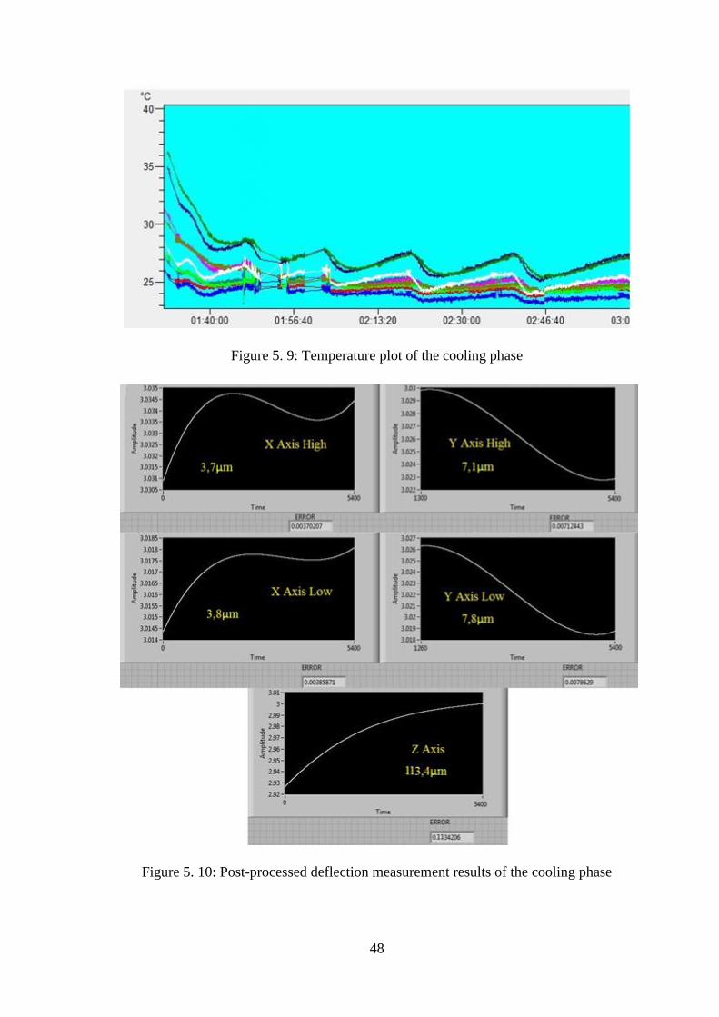
48
Figure 5. 9: Temperature plot of the cooling phase
Figure 5. 10: Post-processed deflection measurement results of the cooling phase
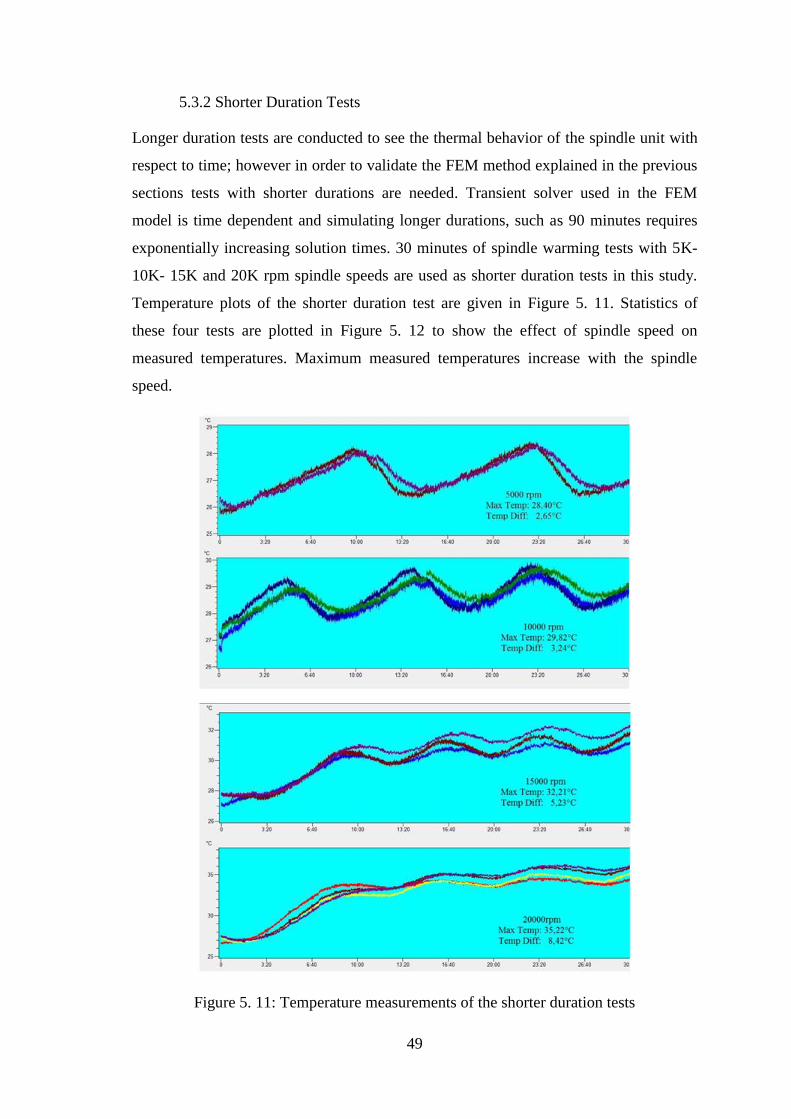
49
5.3.2 Shorter Duration Tests
Longer duration tests are conducted to see the thermal behavior of the spindle unit with
respect to time; however in order to validate the FEM method explained in the previous
sections tests with shorter durations are needed. Transient solver used in the FEM
model is time dependent and simulating longer durations, such as 90 minutes requires
exponentially increasing solution times. 30 minutes of spindle warming tests with 5K-
10K- 15K and 20K rpm spindle speeds are used as shorter duration tests in this study.
Temperature plots of the shorter duration test are given in Figure 5. 11. Statistics of
these four tests are plotted in Figure 5. 12 to show the effect of spindle speed on
measured temperatures. Maximum measured temperatures increase with the spindle
speed.
Figure 5. 11: Temperature measurements of the shorter duration tests
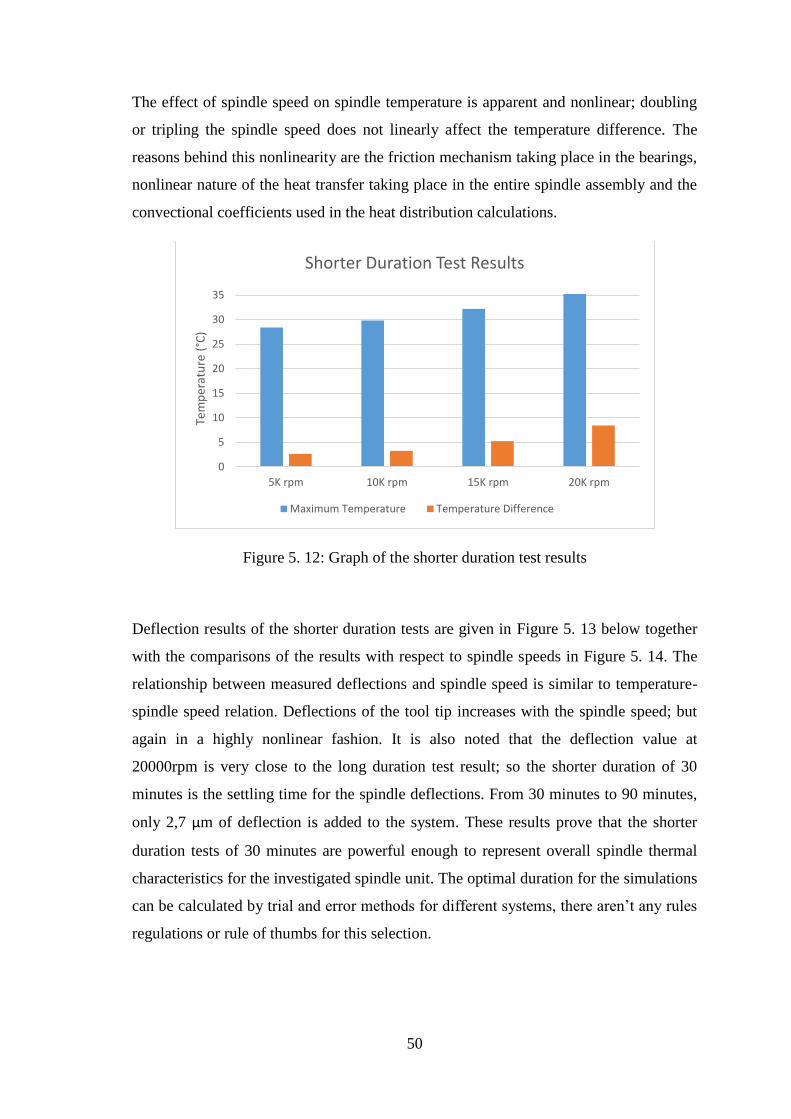
50
The effect of spindle speed on spindle temperature is apparent and nonlinear; doubling
or tripling the spindle speed does not linearly affect the temperature difference. The
reasons behind this nonlinearity are the friction mechanism taking place in the bearings,
nonlinear nature of the heat transfer taking place in the entire spindle assembly and the
convectional coefficients used in the heat distribution calculations.
Figure 5. 12: Graph of the shorter duration test results
Deflection results of the shorter duration tests are given in Figure 5. 13 below together
with the comparisons of the results with respect to spindle speeds in Figure 5. 14. The
relationship between measured deflections and spindle speed is similar to temperature-
spindle speed relation. Deflections of the tool tip increases with the spindle speed; but
again in a highly nonlinear fashion. It is also noted that the deflection value at
20000rpm is very close to the long duration test result; so the shorter duration of 30
minutes is the settling time for the spindle deflections. From 30 minutes to 90 minutes,
only 2,7 µm of deflection is added to the system. These results prove that the shorter
duration tests of 30 minutes are powerful enough to represent overall spindle thermal
characteristics for the investigated spindle unit. The optimal duration for the simulations
can be calculated by trial and error methods for different systems, there aren’t any rules
regulations or rule of thumbs for this selection.
0
5
10
15
20
25
30
35
5K rpm 10K rpm 15K rpm 20K rpm
Tem
per
atu
re (
°C)
Shorter Duration Test Results
Maximum Temperature Temperature Difference
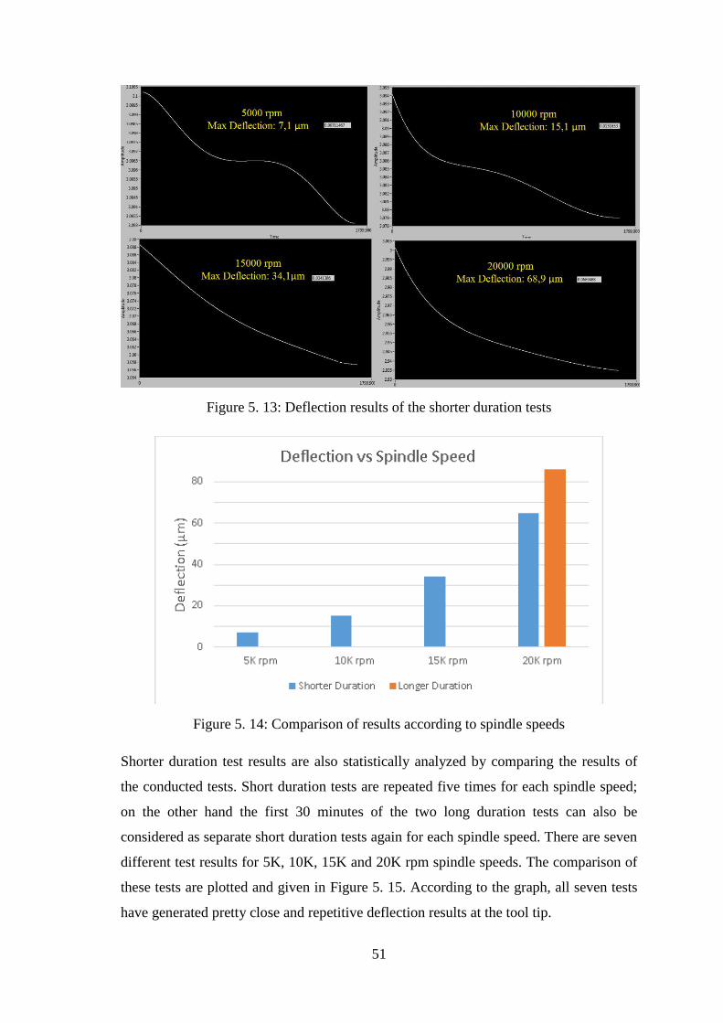
51
Figure 5. 13: Deflection results of the shorter duration tests
Figure 5. 14: Comparison of results according to spindle speeds
Shorter duration test results are also statistically analyzed by comparing the results of
the conducted tests. Short duration tests are repeated five times for each spindle speed;
on the other hand the first 30 minutes of the two long duration tests can also be
considered as separate short duration tests again for each spindle speed. There are seven
different test results for 5K, 10K, 15K and 20K rpm spindle speeds. The comparison of
these tests are plotted and given in Figure 5. 15. According to the graph, all seven tests
have generated pretty close and repetitive deflection results at the tool tip.
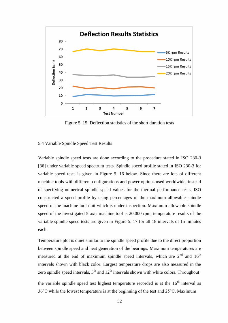
52
Figure 5. 15: Deflection statistics of the short duration tests
5.4 Variable Spindle Speed Test Results
Variable spindle speed tests are done according to the procedure stated in ISO 230-3
[36] under variable speed spectrum tests. Spindle speed profile stated in ISO 230-3 for
variable speed tests is given in Figure 5. 16 below. Since there are lots of different
machine tools with different configurations and power options used worldwide, instead
of specifying numerical spindle speed values for the thermal performance tests, ISO
constructed a speed profile by using percentages of the maximum allowable spindle
speed of the machine tool unit which is under inspection. Maximum allowable spindle
speed of the investigated 5 axis machine tool is 20,000 rpm, temperature results of the
variable spindle speed tests are given in Figure 5. 17 for all 18 intervals of 15 minutes
each.
Temperature plot is quiet similar to the spindle speed profile due to the direct proportion
between spindle speed and heat generation of the bearings. Maximum temperatures are
measured at the end of maximum spindle speed intervals, which are 2nd
and 16th
intervals shown with black color. Largest temperature drops are also measured in the
zero spindle speed intervals, 5th
and 12th
intervals shown with white colors. Throughout
the variable spindle speed test highest temperature recorded is at the 16th
interval as
36°C while the lowest temperature is at the beginning of the test and 25°C. Maximum
0
10
20
30
40
50
60
70
80
1 2 3 4 5 6 7
De
fle
ctio
n (
µm
)
Test Number
Deflection Results Statistics
5K rpm Results
10K rpm Results
15K rpm Results
20K rpm Results
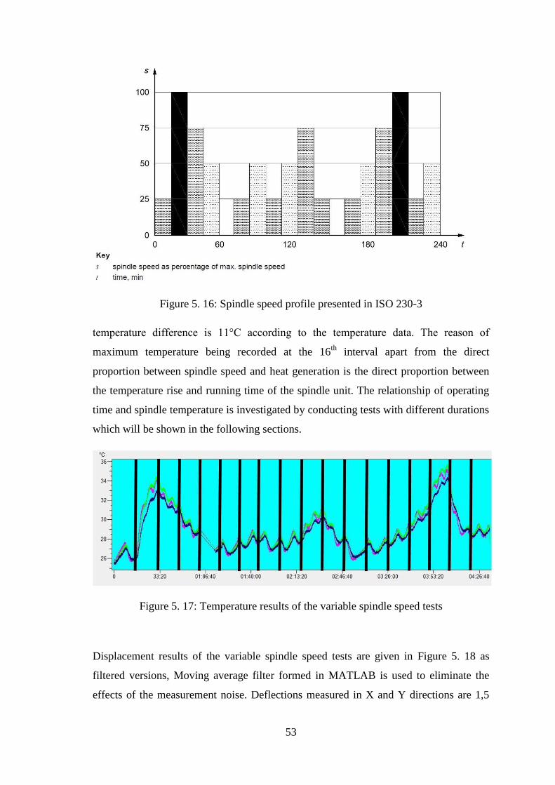
53
Figure 5. 16: Spindle speed profile presented in ISO 230-3
temperature difference is 11°C according to the temperature data. The reason of
maximum temperature being recorded at the 16th
interval apart from the direct
proportion between spindle speed and heat generation is the direct proportion between
the temperature rise and running time of the spindle unit. The relationship of operating
time and spindle temperature is investigated by conducting tests with different durations
which will be shown in the following sections.
Figure 5. 17: Temperature results of the variable spindle speed tests
Displacement results of the variable spindle speed tests are given in Figure 5. 18 as
filtered versions, Moving average filter formed in MATLAB is used to eliminate the
effects of the measurement noise. Deflections measured in X and Y directions are 1,5
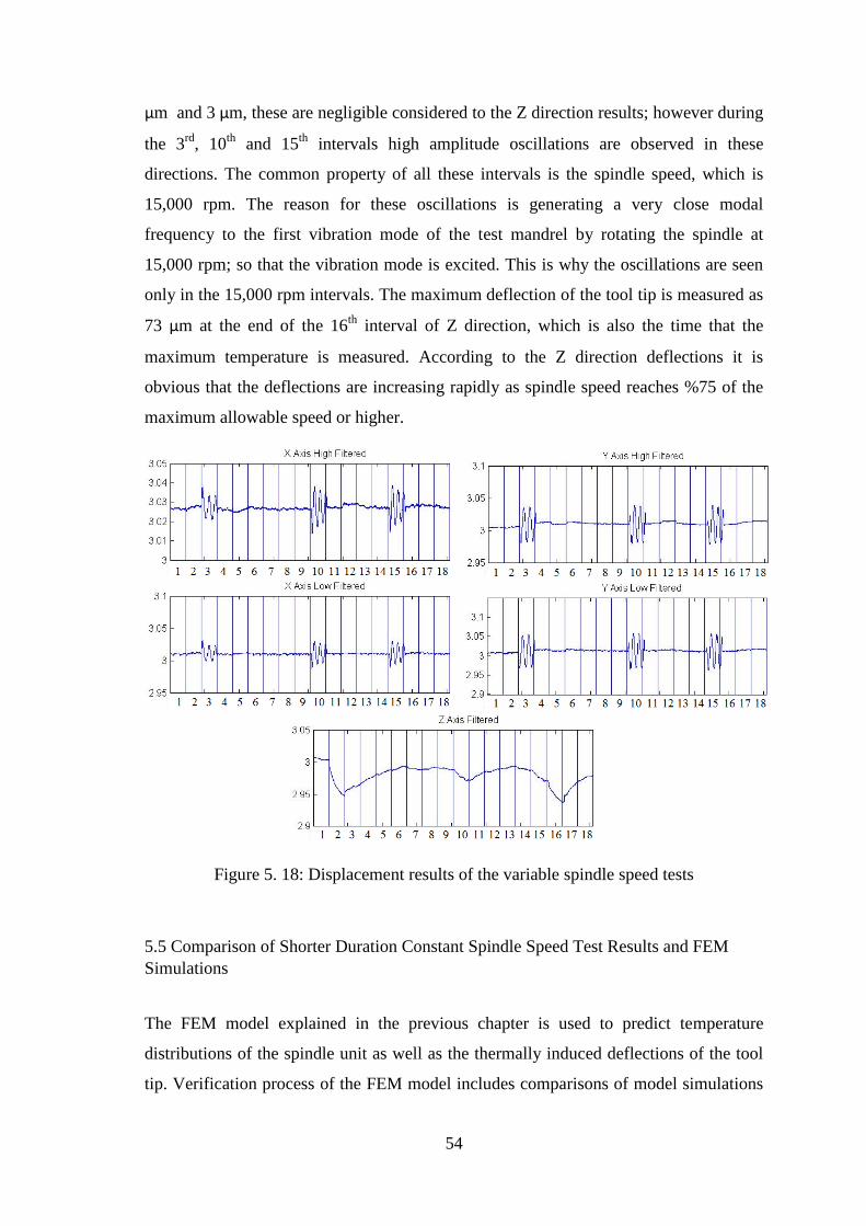
54
µm and 3 µm, these are negligible considered to the Z direction results; however during
the 3rd
, 10th
and 15th
intervals high amplitude oscillations are observed in these
directions. The common property of all these intervals is the spindle speed, which is
15,000 rpm. The reason for these oscillations is generating a very close modal
frequency to the first vibration mode of the test mandrel by rotating the spindle at
15,000 rpm; so that the vibration mode is excited. This is why the oscillations are seen
only in the 15,000 rpm intervals. The maximum deflection of the tool tip is measured as
73 µm at the end of the 16th
interval of Z direction, which is also the time that the
maximum temperature is measured. According to the Z direction deflections it is
obvious that the deflections are increasing rapidly as spindle speed reaches %75 of the
maximum allowable speed or higher.
Figure 5. 18: Displacement results of the variable spindle speed tests
5.5 Comparison of Shorter Duration Constant Spindle Speed Test Results and FEM
Simulations
The FEM model explained in the previous chapter is used to predict temperature
distributions of the spindle unit as well as the thermally induced deflections of the tool
tip. Verification process of the FEM model includes comparisons of model simulations
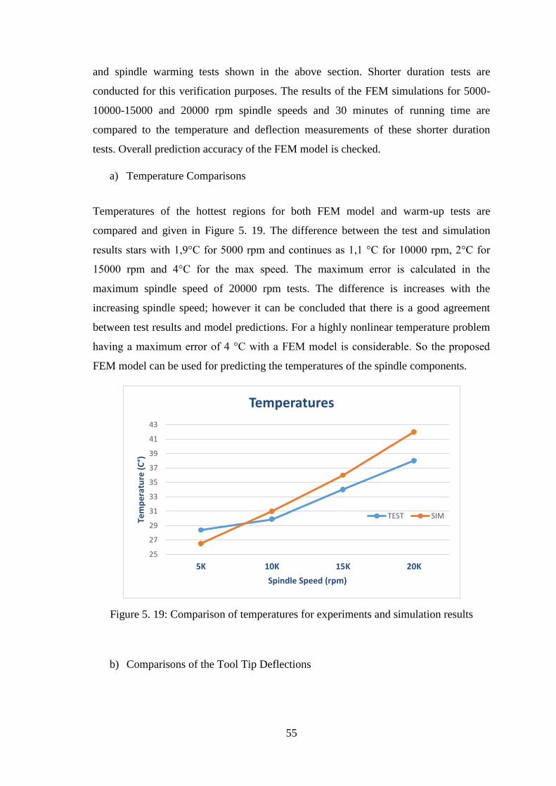
55
and spindle warming tests shown in the above section. Shorter duration tests are
conducted for this verification purposes. The results of the FEM simulations for 5000-
10000-15000 and 20000 rpm spindle speeds and 30 minutes of running time are
compared to the temperature and deflection measurements of these shorter duration
tests. Overall prediction accuracy of the FEM model is checked.
a) Temperature Comparisons
Temperatures of the hottest regions for both FEM model and warm-up tests are
compared and given in Figure 5. 19. The difference between the test and simulation
results stars with 1,9°C for 5000 rpm and continues as 1,1 °C for 10000 rpm, 2°C for
15000 rpm and 4°C for the max speed. The maximum error is calculated in the
maximum spindle speed of 20000 rpm tests. The difference is increases with the
increasing spindle speed; however it can be concluded that there is a good agreement
between test results and model predictions. For a highly nonlinear temperature problem
having a maximum error of 4 °C with a FEM model is considerable. So the proposed
FEM model can be used for predicting the temperatures of the spindle components.
Figure 5. 19: Comparison of temperatures for experiments and simulation results
b) Comparisons of the Tool Tip Deflections
25
27
29
31
33
35
37
39
41
43
5K 10K 15K 20K
Tem
pe
ratu
re (
C°)
Spindle Speed (rpm)
Temperatures
TEST SIM
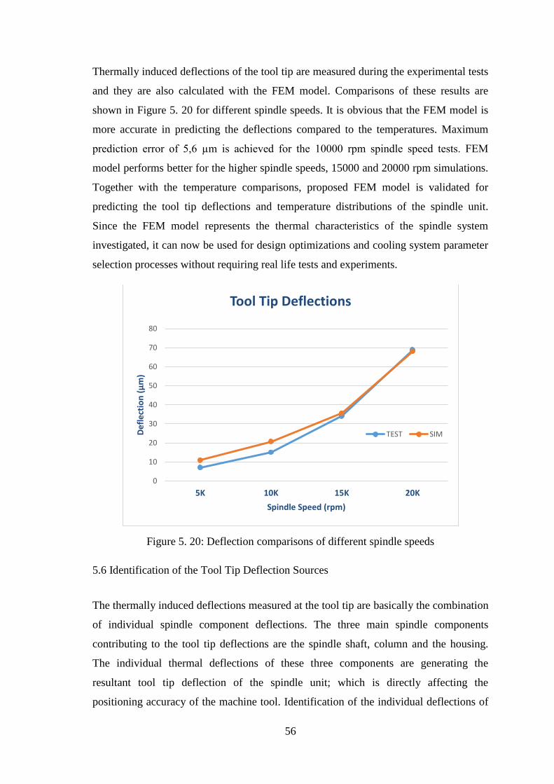
56
Thermally induced deflections of the tool tip are measured during the experimental tests
and they are also calculated with the FEM model. Comparisons of these results are
shown in Figure 5. 20 for different spindle speeds. It is obvious that the FEM model is
more accurate in predicting the deflections compared to the temperatures. Maximum
prediction error of 5,6 µm is achieved for the 10000 rpm spindle speed tests. FEM
model performs better for the higher spindle speeds, 15000 and 20000 rpm simulations.
Together with the temperature comparisons, proposed FEM model is validated for
predicting the tool tip deflections and temperature distributions of the spindle unit.
Since the FEM model represents the thermal characteristics of the spindle system
investigated, it can now be used for design optimizations and cooling system parameter
selection processes without requiring real life tests and experiments.
Figure 5. 20: Deflection comparisons of different spindle speeds
5.6 Identification of the Tool Tip Deflection Sources
The thermally induced deflections measured at the tool tip are basically the combination
of individual spindle component deflections. The three main spindle components
contributing to the tool tip deflections are the spindle shaft, column and the housing.
The individual thermal deflections of these three components are generating the
resultant tool tip deflection of the spindle unit; which is directly affecting the
positioning accuracy of the machine tool. Identification of the individual deflections of
0
10
20
30
40
50
60
70
80
5K 10K 15K 20K
De
fle
ctio
n (
µm
)
Spindle Speed (rpm)
Tool Tip Deflections
TEST SIM
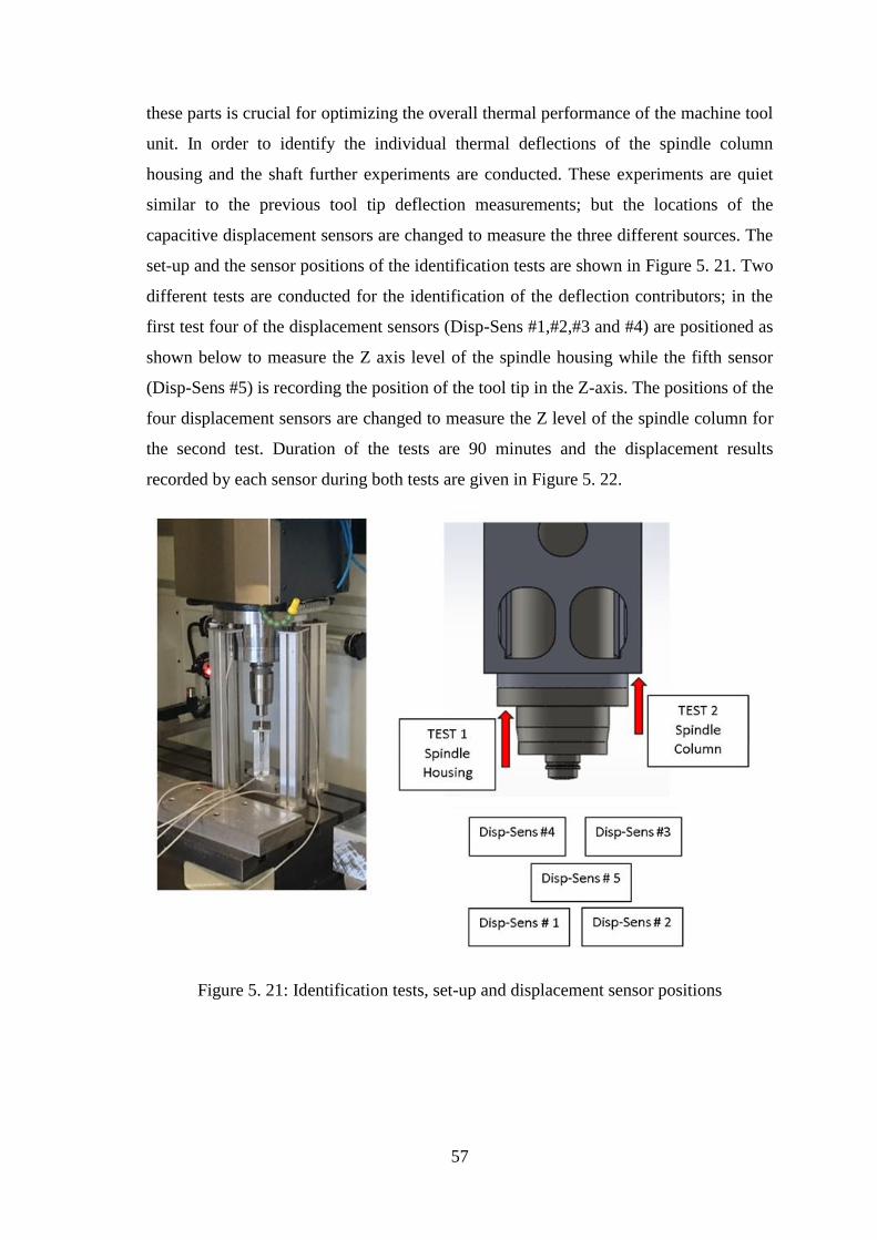
57
these parts is crucial for optimizing the overall thermal performance of the machine tool
unit. In order to identify the individual thermal deflections of the spindle column
housing and the shaft further experiments are conducted. These experiments are quiet
similar to the previous tool tip deflection measurements; but the locations of the
capacitive displacement sensors are changed to measure the three different sources. The
set-up and the sensor positions of the identification tests are shown in Figure 5. 21. Two
different tests are conducted for the identification of the deflection contributors; in the
first test four of the displacement sensors (Disp-Sens #1,#2,#3 and #4) are positioned as
shown below to measure the Z axis level of the spindle housing while the fifth sensor
(Disp-Sens #5) is recording the position of the tool tip in the Z-axis. The positions of the
four displacement sensors are changed to measure the Z level of the spindle column for
the second test. Duration of the tests are 90 minutes and the displacement results
recorded by each sensor during both tests are given in Figure 5. 22.
Figure 5. 21: Identification tests, set-up and displacement sensor positions
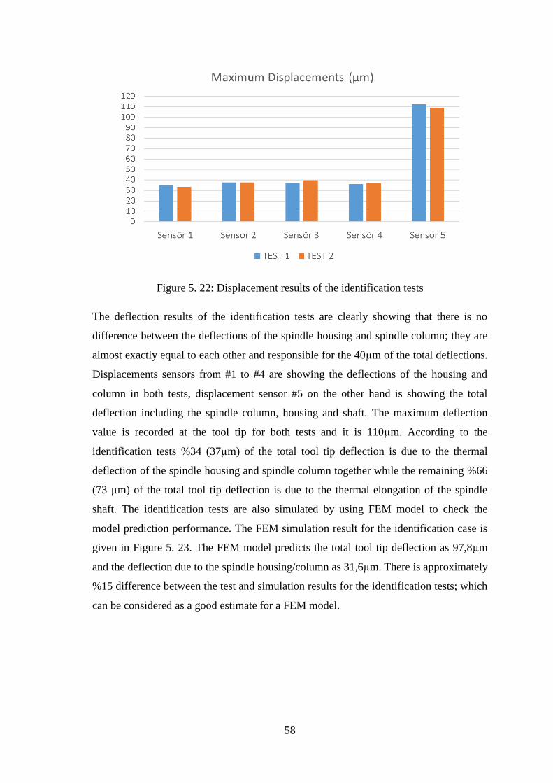
58
Figure 5. 22: Displacement results of the identification tests
The deflection results of the identification tests are clearly showing that there is no
difference between the deflections of the spindle housing and spindle column; they are
almost exactly equal to each other and responsible for the 40µm of the total deflections.
Displacements sensors from #1 to #4 are showing the deflections of the housing and
column in both tests, displacement sensor #5 on the other hand is showing the total
deflection including the spindle column, housing and shaft. The maximum deflection
value is recorded at the tool tip for both tests and it is 110µm. According to the
identification tests %34 (37µm) of the total tool tip deflection is due to the thermal
deflection of the spindle housing and spindle column together while the remaining %66
(73 µm) of the total tool tip deflection is due to the thermal elongation of the spindle
shaft. The identification tests are also simulated by using FEM model to check the
model prediction performance. The FEM simulation result for the identification case is
given in Figure 5. 23. The FEM model predicts the total tool tip deflection as 97,8µm
and the deflection due to the spindle housing/column as 31,6µm. There is approximately
%15 difference between the test and simulation results for the identification tests; which
can be considered as a good estimate for a FEM model.
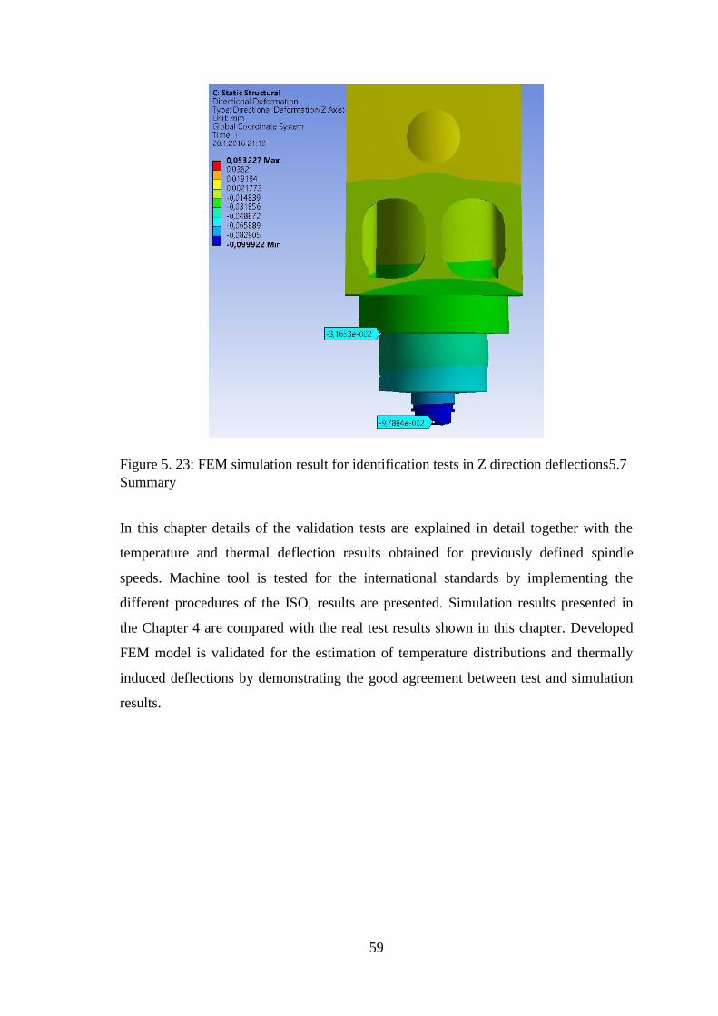
59
Figure 5. 23: FEM simulation result for identification tests in Z direction deflections5.7
Summary
In this chapter details of the validation tests are explained in detail together with the
temperature and thermal deflection results obtained for previously defined spindle
speeds. Machine tool is tested for the international standards by implementing the
different procedures of the ISO, results are presented. Simulation results presented in
the Chapter 4 are compared with the real test results shown in this chapter. Developed
FEM model is validated for the estimation of temperature distributions and thermally
induced deflections by demonstrating the good agreement between test and simulation
results.
60
CHAPTER 6
6. COOLING SYSTEM OPTIMIZATIONS
6.1 Introduction
Cooling system is one of the most important factors affecting the thermally induced
errors of the machine tool spindle systems. Heat generated by the rotating components
and electrical circuits are all removed by the cooling system. Previously introduced
FEM spindle thermal model is proved to be accurate in predicting the heat distributions
and thermal elongations. In this chapter this FEM model is used to simulate the
performance of the cooling system. Cooling system is investigated and optimized in two
different steps; first step is to find optimal cooling system parameters without changing
the design or components while second step is to determine the optimal cooling channel
design to achieve better temperature distributions. For both steps FEM model is used
and simulation results for the previously investigated cases are compared. According to
the results of these simulations further design recommendations are prepared for the
new, thermally stable machine tool spindle unit.
6.2 Parameter Optimizations
Cooling system performance depends not only on the components used in the system
but also to the parameters used in the cooling system. It is possible to achieve better
cooling performance from the same cooling unit with different and optimized
61
parameters. The 5 axis machine tool investigated in this study has a standard cooling
system as explained in detail in the previous chapters. The problem with this cooling
system is that the fluid pump used within the unit is a constant output (non-
programmable) pump; so that the pressure, velocity or the flux of the cooling fluid
cannot be changed. In the parameter optimization studies, FEM thermal spindle model
introduced throughout this thesis is used to simulate the effects of different cooling fluid
inputs; such as fluid velocity entering the cooling channels, pressure of the cooling fluid
within the cooling channels or the initial temperature of the cooling fluid. By the help of
these simulations optimized parameters are found and possible cooling performance
improvements are predicted. The optimized cooling system parameters can be
implemented to the current system by changing only the fluid pump within the cooling
system.
a) Effect of Cooling Fluid Velocity
The velocity of the cooling fluid entering to the machine tool spindle is a critical factor
for the overall cooling system. There are some constraints for the fluid velocity due to
the power of the pump used, cooling channel geometry and efficiency. Higher fluid
velocities are of course better for the cooling performance; but there are some physical
limitations to that. The effect of the fluid velocity is investigated through the FEM
model constructed in the study. The default value for the fluid velocity is 0.4 m/s, in
order to find out the effect of the fluid velocity in both higher and lower velocity cases
are simulated. Velocities chosen for these simulations are 0.08m/s, 0.8 m/s, 2 m/s and 4
m/s respectively. Simulations are conducted for the 20K rpm spindle speed case; since it
has the smallest estimation error by the FEM model for the tool deflection. Comparison
graph of the results are plotted and provided in Figure 6. 1 and Figure 6. 2. The effect of
the cooling fluid velocity on the tool tip deflections and maximum temperatures is
obvious, higher fluid velocity results in lower temperatures and less deflections at the
tool tip accordingly. Increasing the velocity of the cooling fluid also increases the heat
transfer coefficient. Increased heat transfer coefficient means that the same amount of
cooling fluid can absorb more heat from the spindle components. This relationship is
previously shown in the heat transfer coefficient calculation of the rotating shaft in
Chapter 3 by equation 15. According to the graphs, it is shown that the cooling
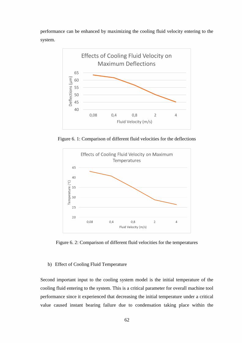
62
performance can be enhanced by maximizing the cooling fluid velocity entering to the
system.
Figure 6. 1: Comparison of different fluid velocities for the deflections
Figure 6. 2: Comparison of different fluid velocities for the temperatures
b) Effect of Cooling Fluid Temperature
Second important input to the cooling system model is the initial temperature of the
cooling fluid entering to the system. This is a critical parameter for overall machine tool
performance since it experienced that decreasing the initial temperature under a critical
value caused instant bearing failure due to condensation taking place within the
40
45
50
55
60
65
0,08 0,4 0,8 2 4
Def
lect
ion
s (µ
m)
Fluid Velocity (m/s)
Effects of Cooling Fluid Velocity on Maximum Deflections
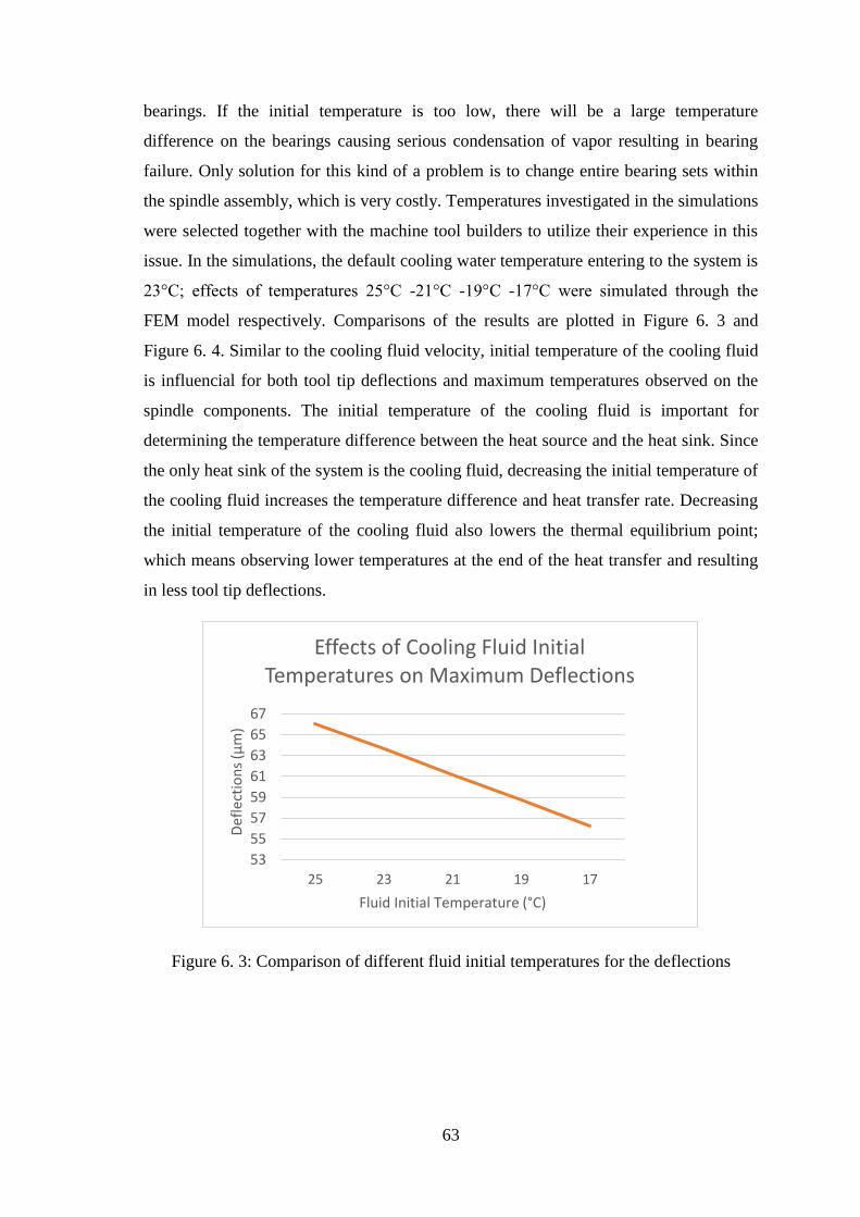
63
bearings. If the initial temperature is too low, there will be a large temperature
difference on the bearings causing serious condensation of vapor resulting in bearing
failure. Only solution for this kind of a problem is to change entire bearing sets within
the spindle assembly, which is very costly. Temperatures investigated in the simulations
were selected together with the machine tool builders to utilize their experience in this
issue. In the simulations, the default cooling water temperature entering to the system is
23°C; effects of temperatures 25°C -21°C -19°C -17°C were simulated through the
FEM model respectively. Comparisons of the results are plotted in Figure 6. 3 and
Figure 6. 4. Similar to the cooling fluid velocity, initial temperature of the cooling fluid
is influencial for both tool tip deflections and maximum temperatures observed on the
spindle components. The initial temperature of the cooling fluid is important for
determining the temperature difference between the heat source and the heat sink. Since
the only heat sink of the system is the cooling fluid, decreasing the initial temperature of
the cooling fluid increases the temperature difference and heat transfer rate. Decreasing
the initial temperature of the cooling fluid also lowers the thermal equilibrium point;
which means observing lower temperatures at the end of the heat transfer and resulting
in less tool tip deflections.
Figure 6. 3: Comparison of different fluid initial temperatures for the deflections
53
55
57
59
61
63
65
67
25 23 21 19 17
Def
lect
ion
s (µ
m)
Fluid Initial Temperature (°C)
Effects of Cooling Fluid Initial Temperatures on Maximum Deflections

64
Figure 6. 4: Comparison of different fluid initial temperatures for the temperatures
6.3 Design Optimization
Cooling system performance can be improved by tuning the system parameters as
shown in the above section. However there are physical limitations to the parameters
that can be tuned to improve the cooling performance. For instance the velocity of the
cooling fluid is limited by the power of the hydraulic pump used in the chiller unit;
similarly the initial temperature of the fluid is limited by the bearing condensation
problem which limits the minimum temperature of the cooling fluid at 18ºC for the
investigated spindle unit.For the spindle cooling systems, design of the cooling channels
are the most important factor on the overall cooling performance. For instance, relative
position of these channels to the main heat sources of the spindle unit, surface areas of
the channels, cross-sections of the channels, locations and amount of the channel
inlets/outlets are some of the important features regarding to the cooling channel design.
For the investigated machine tool spindle unit, current channel geometry is modified in
the simulations considering several cooling channel designs from the literature. Some of
the FEM model simulations are repeated with the new channel embedded spindle CAD
models. Temperature distributions and the resulting thermal deformations are compared
with the current design. According to the results of these simulations further design
recommendations are outlined to be used in the completely new, thermally stable
spindle design.
43
44
45
46
47
48
49
50
25 23 21 19 17
Tem
per
atu
re (
ºC)
Fluid Initial Temperature (°C)
Effects of Cooling Fluid Initial Temperatures on Temperatures
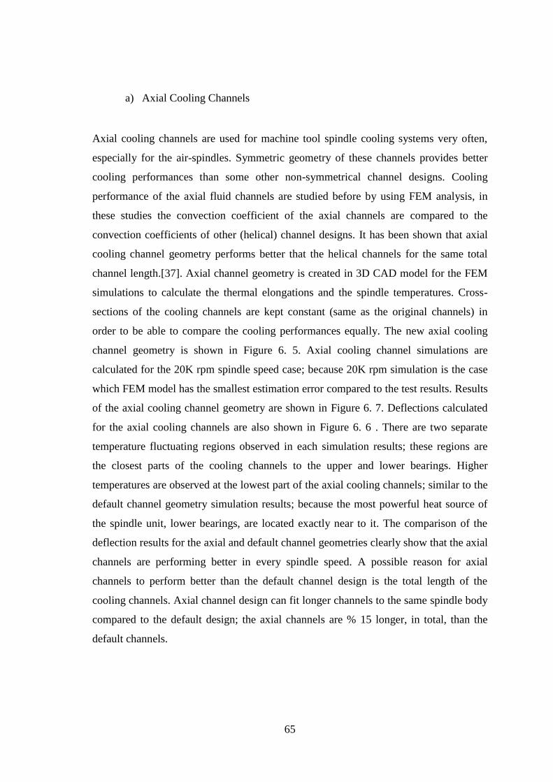
65
a) Axial Cooling Channels
Axial cooling channels are used for machine tool spindle cooling systems very often,
especially for the air-spindles. Symmetric geometry of these channels provides better
cooling performances than some other non-symmetrical channel designs. Cooling
performance of the axial fluid channels are studied before by using FEM analysis, in
these studies the convection coefficient of the axial channels are compared to the
convection coefficients of other (helical) channel designs. It has been shown that axial
cooling channel geometry performs better that the helical channels for the same total
channel length.[37]. Axial channel geometry is created in 3D CAD model for the FEM
simulations to calculate the thermal elongations and the spindle temperatures. Cross-
sections of the cooling channels are kept constant (same as the original channels) in
order to be able to compare the cooling performances equally. The new axial cooling
channel geometry is shown in Figure 6. 5. Axial cooling channel simulations are
calculated for the 20K rpm spindle speed case; because 20K rpm simulation is the case
which FEM model has the smallest estimation error compared to the test results. Results
of the axial cooling channel geometry are shown in Figure 6. 7. Deflections calculated
for the axial cooling channels are also shown in Figure 6. 6 . There are two separate
temperature fluctuating regions observed in each simulation results; these regions are
the closest parts of the cooling channels to the upper and lower bearings. Higher
temperatures are observed at the lowest part of the axial cooling channels; similar to the
default channel geometry simulation results; because the most powerful heat source of
the spindle unit, lower bearings, are located exactly near to it. The comparison of the
deflection results for the axial and default channel geometries clearly show that the axial
channels are performing better in every spindle speed. A possible reason for axial
channels to perform better than the default channel design is the total length of the
cooling channels. Axial channel design can fit longer channels to the same spindle body
compared to the default design; the axial channels are % 15 longer, in total, than the
default channels.
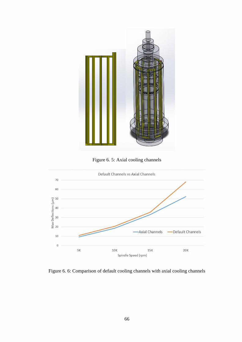
66
Figure 6. 5: Axial cooling channels
Figure 6. 6: Comparison of default cooling channels with axial cooling channels
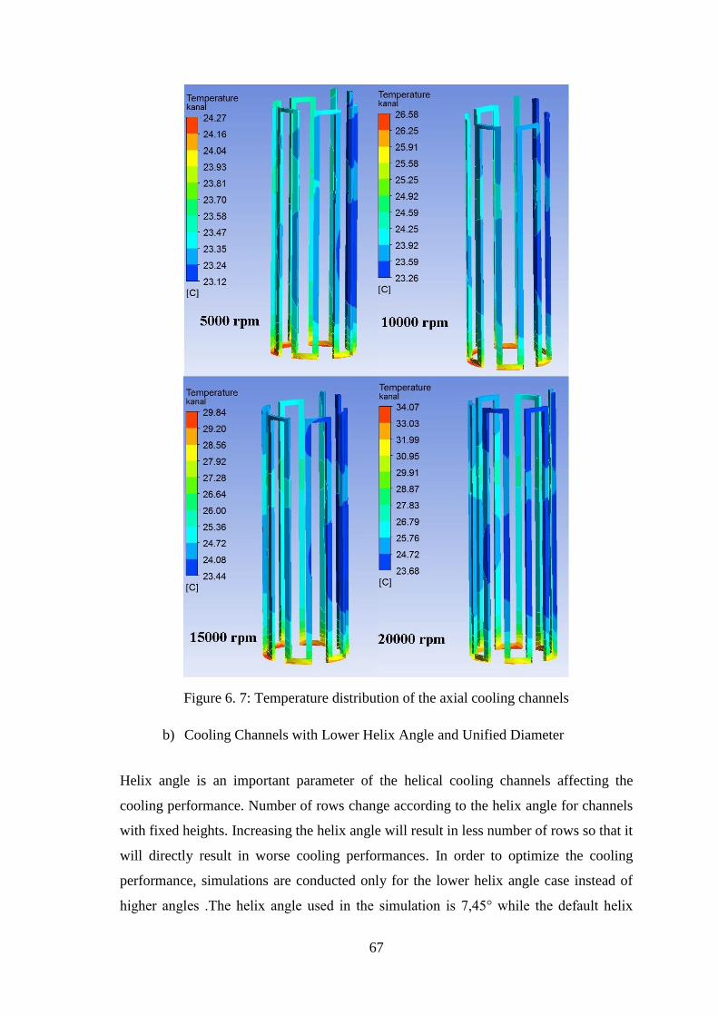
67
Figure 6. 7: Temperature distribution of the axial cooling channels
b) Cooling Channels with Lower Helix Angle and Unified Diameter
Helix angle is an important parameter of the helical cooling channels affecting the
cooling performance. Number of rows change according to the helix angle for channels
with fixed heights. Increasing the helix angle will result in less number of rows so that it
will directly result in worse cooling performances. In order to optimize the cooling
performance, simulations are conducted only for the lower helix angle case instead of
higher angles .The helix angle used in the simulation is 7,45° while the default helix
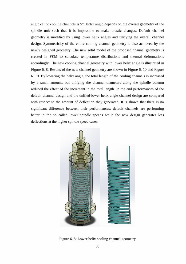
68
angle of the cooling channels is 9°. Helix angle depends on the overall geometry of the
spindle unit such that it is impossible to make drastic changes. Default channel
geometry is modified by using lower helix angles and unifying the overall channel
design. Symmetricity of the entire cooling channel geometry is also achieved by the
newly designed geometry. The new solid model of the proposed channel geometry is
created in FEM to calculate temperature distributions and thermal deformations
accordingly. The new cooling channel geometry with lower helix angle is illustrated in
Figure 6. 8. Results of the new channel geometry are shown in Figure 6. 10 and Figure
6. 10. By lowering the helix angle, the total length of the cooling channels is increased
by a small amount; but unifying the channel diameters along the spindle column
reduced the effect of the increment in the total length. In the end performances of the
default channel design and the unified-lower helix angle channel design are compared
with respect to the amount of deflection they generated. It is shown that there is no
significant difference between their performances; default channels are performing
better in the so called lower spindle speeds while the new design generates less
deflections at the higher spindle speed cases.
Figure 6. 8: Lower helix cooling channel geometry
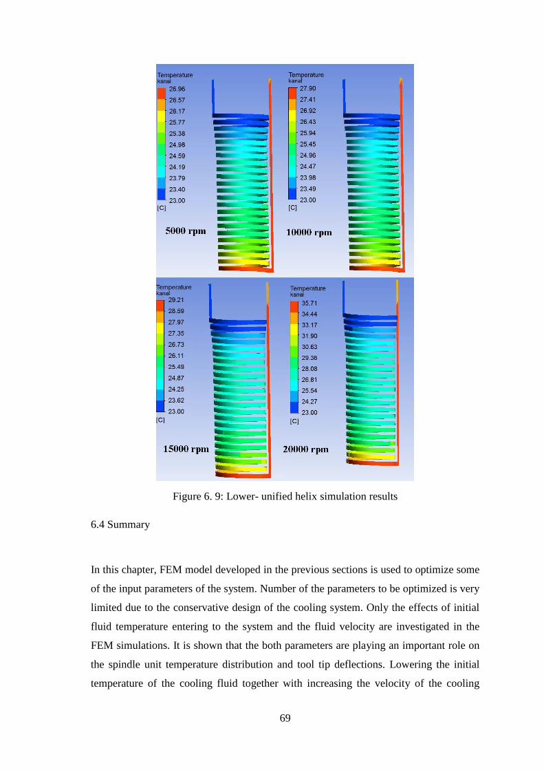
69
Figure 6. 9: Lower- unified helix simulation results
6.4 Summary
In this chapter, FEM model developed in the previous sections is used to optimize some
of the input parameters of the system. Number of the parameters to be optimized is very
limited due to the conservative design of the cooling system. Only the effects of initial
fluid temperature entering to the system and the fluid velocity are investigated in the
FEM simulations. It is shown that the both parameters are playing an important role on
the spindle unit temperature distribution and tool tip deflections. Lowering the initial
temperature of the cooling fluid together with increasing the velocity of the cooling
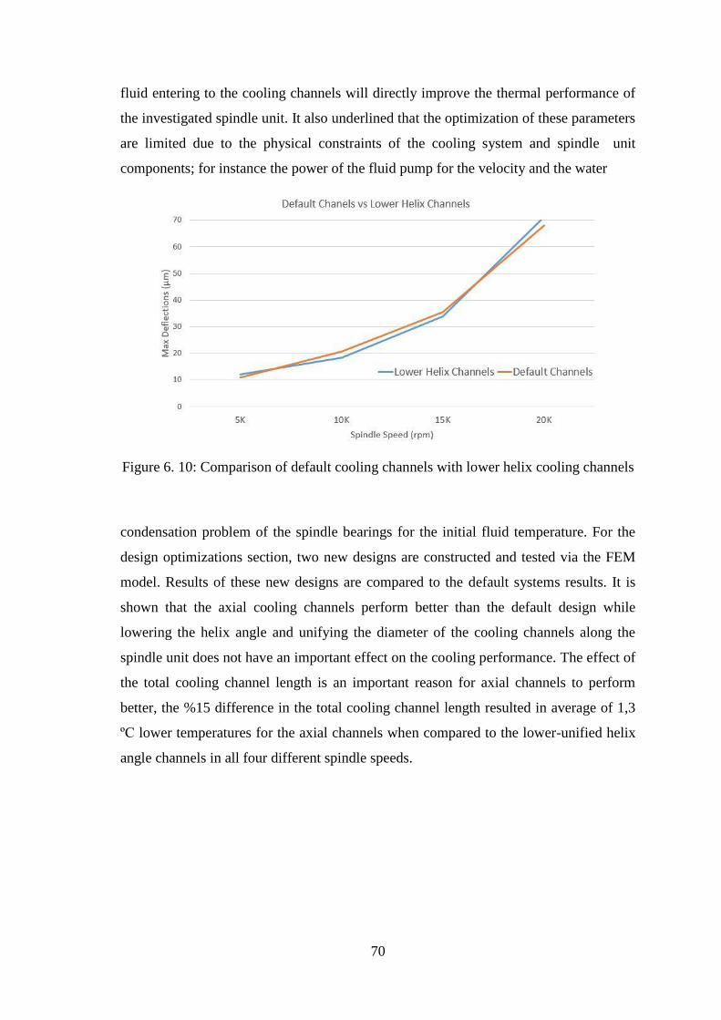
70
fluid entering to the cooling channels will directly improve the thermal performance of
the investigated spindle unit. It also underlined that the optimization of these parameters
are limited due to the physical constraints of the cooling system and spindle unit
components; for instance the power of the fluid pump for the velocity and the water
Figure 6. 10: Comparison of default cooling channels with lower helix cooling channels
condensation problem of the spindle bearings for the initial fluid temperature. For the
design optimizations section, two new designs are constructed and tested via the FEM
model. Results of these new designs are compared to the default systems results. It is
shown that the axial cooling channels perform better than the default design while
lowering the helix angle and unifying the diameter of the cooling channels along the
spindle unit does not have an important effect on the cooling performance. The effect of
the total cooling channel length is an important reason for axial channels to perform
better, the %15 difference in the total cooling channel length resulted in average of 1,3
ºC lower temperatures for the axial channels when compared to the lower-unified helix
angle channels in all four different spindle speeds.

71
CHAPTER 7
7. SUGGESTIONS FOR FURTHER RESEARCH
Thermal aspects of a 5 axis vertical machine tool spindle unit are analyzed by the
constructed FEM model throughout the study. The performance of the FEM model is
validated by the measurements; however there are still some points of improvement for
the study. Following recommendations may improve the presented model in the means
of prediction accuracy, robustness and calculation times:
Heat sources used in the presented FEM model can be extended by including the
heat generated by the motor, heat generated by the moving axes and heat
generated in the ball-screws in order to represent all of the possible heat sources
in a machine tool. The only heat source used in the presented model is the heat
generated by the spindle bearings; due to the fact that the most of the heat
generated in the machine tool is generated by the spindle bearings. Adding other
heat sources may increase the model complexity and calculation times.
The effect of the additional cooling systems, such as through coolant may be
included to the model to see if there is a drastic improvement in the thermal
behavior of the machine tool.
Optimizations presented in this study are only based on the current spindle
design (cooling channel cross sections are kept constant, location of the channels
are kept constant…etc.); however completely new channel designs may be
simulated for increasing the thermal performance of the machine tool.
Parameter optimizations are also limited by the physical properties of the current
cooling system. The only parameters that can be tuned are used for optimization

72
purposes; but the number of parameters that can be tuned may be increased by
changing the physical properties of the cooling system. Simulations may be
extended to see the amount of improvement for changing the cooling unit with a
new, more powerful and adjustable cooling unit.
The effect of the material properties of the spindle unit components are not
investigated in this study; however it is know that the thermal behavior is highly
depending on the material properties. Simulations may be extended by
considering different material for the spindle unit components. System
optimization may be achieved by better material selection.
73
CHAPTER 8
8. DISCUSSIONS AND CONCLUSIONS
High speed spindle units are inseparable components of the current machine tools used
in precision machining industries. Demand for tighter tolerances together with lower
scrap ratios and minimal costs are increasing rapidly as the technology develops. In
order to satisfy these demands, manufacturing industry needs faster, more accurate and
more efficient machine tools. Main aim of this thesis was to develop a practical tool for
machine tool users to estimate thermal performance of the machine tools easily.
Conclusions and the contributions of the thesis are as following:
It is shown that the heat generated at the angular contact bearings is directly
proportional to the applied loads and the spindle speed; but there is no linear
trend between these parameters and the temperature distributions.
The importance of bearing selection, deciding the bearing diameter and the
amount of the preload that is going to be applied on these bearings, is
emphasized by showing the effects of both bearing diameters and the preloads
on the generated bearing heat.
It is shown that the accurate prediction of the machine tool spindle temperature
distributions can be achieved by modelling the most important heat sources
within the spindle assembly, spindle bearings.
The relationship between the temperature distribution and the thermally induced
errors are underlined by the conducted experiments and FEM simulations; so
74
that by reducing both the maximum temperature value and its accumulation near
to the tool tip, thermal performance can be enhanced.
The velocity and the initial temperature of the cooling fluid used in the cooling
system are influential on the final thermally induced errors and these parameters
are needed to be tuned.
Performance of the cooling system can be enhanced by simply changing the
channel geometry, without changing the cross-sections or the flow rate.
Developed FEM model in this study is a generic model which can be used with
any other spindle and cooling system designs by simply uploading the 3D CAD
model of the new spindle unit to be tested. This feature enables machine tool
builders, Spinner Machine Tools in the context of this study, to simulate their
prototype designs for better cooling performances.
By using the developed FEM model both design and parameter optimizations
can be done for the machine tools. External parameters of the cooling system
such as the power of the fluid pump, pressure of the cooling fluid or the set
temperature of the cooling fluid can be tuned by conducting several simulations.
Spindle design on the other hand can also be optimized by simulating the
temperature distributions and the thermal deformations of various possible
designs as shown by simulating axial and lower helixed cooling channel designs
in chapter 6.
75
REFERENCES
[1] Bryan, J. International status of thermal error research. (keynote) CIRP Annals
16, (1968)
[2] Bryan, J., Pearson, J., Machine tool metrology. ASTME Conf. Sun Francisco,
UCRL 71164 (1968)
[3] Bryan, J., Clouser, R., and McClure, E.. Expansion of a cutting tool during chip
removal. CIRP Annals 16, (1968)
[4] Bryan, J., Donaldson, R., Clouser, R., Blewett W., Reduction of machine tool
spindle growth. NAMRC, McMasters Univ. UCRL 74672 (1973)
[5] Sata, T., Takeuchi, Y., Sakamoto, M., & Weck, M. (1981). Improvement of working
accuracy on NC lathe by compensation for the thermal expansion of tool. CIRP Annals-
Manufacturing Technology, 30(1), 445-449.
[6] Weck, M., et al. "Reduction and compensation of thermal errors in machine tools."
CIRP Annals-Manufacturing Technology 44.2 (1995): 589-598.
[7] Wang, Y., Zhang, G., Moon, K. S., & Sutherland, J. W. (1998). Compensation for
the thermal error of a multi-axis machining center. Journal of materials processing
technology, 75(1), 45-53.
[8] Mou, J., M. A. Donmez, and S. Cetinkunt. "An adaptive error correction method
using feature-based analysis techniques for machine performance improvement, Part 1:
Theory derivation." Journal of Manufacturing Science and Engineering 117.4 (1995):
584-590.
[9] Moriwaki, Toshimichi, and Eiji Shamoto. "Analysis of thermal deformation of an
ultraprecision air spindle system." CIRP Annals-Manufacturing Technology 47.1
(1998): 315-319.
[10] Haitao, Zhao, Yang Jianguo, and Shen Jinhua. "Simulation of thermal behavior
of a CNC machine tool spindle." International Journal of Machine Tools and
Manufacture 47.6 (2007): 1003-1010.
[11] Chen, Shao-Hsien, Chin-Mou Hsu, and Yi-Lang Tsai. "Measurement Technique
of Thermal Temperature Rise of Double Column Machining Center." International
Journal of Engineering and Industries 5.1 (2014): 48.
[12] Wang, Yung-Cheng, Ming-che Kao, and Chung-Ping Chang. "Investigation on
the spindle thermal displacement and its compensation of precision cutter grinders."
Measurement 44.6 (2011): 1183-1187.
[13] Li, Shuhe, Yiqun Zhang, and Guoxiong Zhang. "A study of pre-compensation
for thermal errors of NC machine tools." International Journal of Machine Tools and
Manufacture 37.12 (1997): 1715-1719.

76
[14] Hattori, M., et al. "Estimation of thermal-deformation in machine tools using
neural network technique." Journal of materials processing technology 56.1 (1996):
765-772.
[15] Vanherck, Paul, J. Dehaes, and Marnix Nuttin. "Compensation of thermal
deformations in machine tools with neural nets." Computers in industry 33.1 (1997):
119-125.
[16] Mize, Christopher D., and John C. Ziegert. "Neural network thermal error
compensation of a machining center." Precision Engineering 24.4 (2000): 338-346.
[17] Palmgren, A., 1959, Ball and Roller Bearing Engineering, S. H. Burbank,
Philadelphia, PA.
[18] Harris, T. A., and M. H. Mindel. "Rolling element bearing dynamics." Wear
23.3 (1973): 311-337.
[19] Burton, R. A., and H. E. Staph. "Thermally activated seizure of angular contact
bearings." ASLE transactions 10.4 (1967): 408-417.
[20] Jorgensen, Bert Ray. "Robust modeling of high-speed spindle-bearing dynamics
under operating conditions." (1996).
[21] Stein, J. L., and Tu, J. F., 1994, ‘‘A State-Space Model for Monitoring
Thermally-Induced Preload in Anti-Friction Spindle Bearings of High-Speed Machine
Tools,’’ASME J. Dyn. Syst., Meas., Control, Sept., pp. 372–386.
[22] B. Bossmanns, J.F. Tu, A power flow model for high speed motorized spindles-
heat generation characterization, Transactions of the ASME, Journal of Manufacturing
Science and Engineering 123 (2001) 494–505.
[23] B. Bossmanns, J.F. Tu, A thermal model for high speed motorized spindles,
International Journal of Machine Tools & Manufacture 39 (1999) 1345–1366.
[24] Li, Hongqi, and Yung C. Shin. "Analysis of bearing configuration effects on
high speed spindles using an integrated dynamic thermo-mechanical spindle model."
International Journal of Machine Tools and Manufacture 44.4 (2004): 347-364.
[25] Li, Hongqi, and Yung C. Shin. "Integrated dynamic thermo-mechanical
modeling of high speed spindles, part 1: model development." Journal of Manufacturing
Science and Engineering 126.1 (2004): 148-158.
[26] Li, Hongqi, and Yung C. Shin. "Integrated dynamic thermo-mechanical
modeling of high speed spindles, part 2: solution procedure and validations." Journal of
manufacturing science and engineering 126.1 (2004): 159-168.
[27] Min, Xu, Jiang Shuyun, and Cai Ying. "An improved thermal model for machine
tool bearings." International Journal of Machine Tools and Manufacture 47.1 (2007):
53-62.
77
[28] Jin, Chao, Bo Wu, and Youmin Hu. "Heat generation modeling of ball bearing
based on internal load distribution." Tribology International 45.1 (2012): 8-15.
[29] SKF Group, “Super-precision angular contact ball bearings: High-speed, B
design, sealed as standard”, Product Catalogue, 2102.
[30] SCHAEFFLER GROUP, “FAG Super Precision Bearings” Issue AC4/130/7EA,
Apr.2008.
[31] Jeng, Yeau-Ren, and Pay-Yau Huang. "Predictions of temperature rise for ball
bearings." Tribology transactions 46.1 (2003): 49-56.
[32] Ashby, M. F., J. Abulawi, and H. S. Kong. "Temperature maps for frictional
heating in dry sliding." Tribology Transactions 34.4 (1991): 577-587.
[33] F.P. Incropera, D.P. De Witt, Fundamentals of heat and mass transfer, 4th Ed.,
John Wiley and Sons, 1996.
[34] FRIEDHELM LOH GROUP, “Catalogue 33 Edition 2011/2012”, RITTAL
GmbH & Co. KG, 2011
[35] ISO 10791-10: 2007, Test conditions for machining centres — Part 10:
Evaluation of thermal distorsions
[36] ISO 230-3:2007, Test code for machine tools -Part 3: Determination of thermal
effects
[37] MadhanMuthuGanesh, K., et al. "CFD Analysis of cooling channels in built-in
motorized high speed spindle."
[38] Yalcin,T.K, Avcı A, M.S, Budak E., “An Experimental Study for Tool Center
Point Displacements of a 5-axis CNC Machine Tool due to Thermal Effects”, 8th
Diemold Conference, 2015
[39] Yalcin,T.K,Erberdi M.S, Özlü E., Budak E., “ Thermal Modeling of High Speed
Spindles”, 6th
National Machining Symposium (UTIS), 2015


![Sayısal Belgelerde Projeksiyon Ölçek Uzayı ile Tablo ... · için geometrik düzen analizi ve mantıksal düzen analizi yapılarak belgenin analizi gerçekletirilebilir[4]. Belge](https://static.fdocuments.in/doc/165x107/5e43b792bcc85a4ded7ea3e9/saysal-belgelerde-projeksiyon-lek-uzay-ile-tablo-iin-geometrik-dzen.jpg)