Technical note: Packington Power Plant: Dispersion of Emissions … · 2020. 9. 4. · Packington...
24
1 © Amec Foster Wheeler Environment & Infrastructure UK Limited June 2015 Doc Ref: S:\E&I\Projects\30356 REM Sita Packington\D - Design\Final_Tech_Note 15379i1.docx Technical note: Packington Power Plant: Dispersion of Emissions to Air from Landfill Gas Engines 1. Introduction Amec Foster Wheeler Environment and Infrastructure UK Ltd (‘Amec Foster Wheeler’) has been commissioned by SITA UK Limited (SITA) to undertake an air quality assessment to determine the impact from the operation of 7 established landfill gas engines, as well as an additional proposed engine, at Packington Power Plant, West Midlands. Following the recent installation of 7 Jenbacher engines from 2012 – 2014, a proposed eighth engine is due to be commissioned. The necessity for Engine 8 has arisen due to the requirement to maintain generation output at 7MW whilst another engine is operating at reduced output or is offline for routine maintenance – Engine 8 will provide additional engine capacity for this to be possible. Initially, the location for the proposed eighth engine was in the Engine House. However due to space constraints, Engine 8 will now be installed at the south end of site. The proposed new engine will be a either a Jenbacher JCG320 or a CAT 3516. In this assessment the model has been developed to identify the maximum likely short-term and long-term impacts on local air quality during operation under a ‘worst -case’ emission scenario. That is to say that it has been assumed that all 8 engines operate continuously throughout the year at maximum load. 1.1 Aims and Objectives The overall aim of this technical note is to present the results of dispersion emissions to air from Packington Power Plant. The impacts of 7 established on-site engines, as well as an eighth proposed engine, have been assessed using detailed dispersion modelling and the H1 methodology. 1.2 Site and Operator The site address is: Packington Power Plant SITA UK Ltd Packington Lane Little Packington West Midlands CV7 7HN Grid Reference: SP213846.
Transcript of Technical note: Packington Power Plant: Dispersion of Emissions … · 2020. 9. 4. · Packington...

1 © Amec Foster Wheeler Environment & Infrastructure UK Limited
June 2015 Doc Ref: S:\E&I\Projects\30356 REM Sita Packington\D - Design\Final_Tech_Note 15379i1.docx
Technical note: Packington Power Plant: Dispersion of Emissions to Air from Landfill Gas Engines
1. Introduction
Amec Foster Wheeler Environment and Infrastructure UK Ltd (‘Amec Foster Wheeler’) has been
commissioned by SITA UK Limited (SITA) to undertake an air quality assessment to determine the impact
from the operation of 7 established landfill gas engines, as well as an additional proposed engine, at
Packington Power Plant, West Midlands.
Following the recent installation of 7 Jenbacher engines from 2012 – 2014, a proposed eighth engine is due
to be commissioned. The necessity for Engine 8 has arisen due to the requirement to maintain generation
output at 7MW whilst another engine is operating at reduced output or is offline for routine maintenance –
Engine 8 will provide additional engine capacity for this to be possible. Initially, the location for the proposed
eighth engine was in the Engine House. However due to space constraints, Engine 8 will now be installed at
the south end of site. The proposed new engine will be a either a Jenbacher JCG320 or a CAT 3516.
In this assessment the model has been developed to identify the maximum likely short-term and long-term
impacts on local air quality during operation under a ‘worst-case’ emission scenario. That is to say that it has
been assumed that all 8 engines operate continuously throughout the year at maximum load.
1.1 Aims and Objectives
The overall aim of this technical note is to present the results of dispersion emissions to air from Packington
Power Plant. The impacts of 7 established on-site engines, as well as an eighth proposed engine, have been
assessed using detailed dispersion modelling and the H1 methodology.
1.2 Site and Operator
The site address is:
Packington Power Plant
SITA UK Ltd
Packington Lane
Little Packington
West Midlands
CV7 7HN
Grid Reference: SP213846.

2 © Amec Foster Wheeler Environment & Infrastructure UK Limited
June 2015 Doc Ref: S:\E&I\Projects\30356 REM Sita Packington\D - Design\Final_Tech_Note 15379i1.docx
The general site location is shown in Figure 1.1 below, the location of the Packington Power Plant (PPP)
compound installation boundary is shown in Figure 1.2, and the layout of the engines in Figure 1.3 (proposed
Engine 8 circled in red).
Figure 1.1 Packington Landfill Site Location
Figure 1.2 Packington Landfill Installation Boundary
Site Location

3 © Amec Foster Wheeler Environment & Infrastructure UK Limited
June 2015 Doc Ref: S:\E&I\Projects\30356 REM Sita Packington\D - Design\Final_Tech_Note 15379i1.docx
Figure 1.3 Packington Power Plant Layout
2. Methodology
2.1 The Dispersion Model
This study uses the ADMS 5.1 model, which was developed in the UK by Cambridge Environmental
Research Consultants (CERC) in collaboration with the Meteorological Office, National Power and the
University of Surrey. ADMS is termed a ‘new generation’ model, parameterising stability and turbulence in
the planetary boundary layer (PBL) by the Monin-Obukhov length and the boundary layer depth. This
approach allows the vertical structure of the PBL to be more accurately defined than by the stability
classification methods of earlier dispersion models such as R91 or ISC.
Like R91 and ISC, ADMS adopts a symmetrical Gaussian profile of the concentration distribution in the
vertical and crosswind directions in neutral and stable conditions. However, unlike R91 or ISC, the ADMS
vertical concentration profile in convective conditions adopts a skewed Gaussian distribution to take account
of the heterogeneous nature of the vertical velocity distribution in the Convective Boundary Layer (CBL).
Numerous model validation studies have demonstrated that ADMS is acknowledged to be fit for the purpose
of EIA and EP by the Environment Agency and planning authorities.
2.2 Process Emissions
This assessment has considered emissions to air from a total of 8 landfill gas engines. For the purposes of
this assessment, emissions of oxides of nitrogen (NOx), carbon monoxide (CO), volatile organic compounds
(VOCs) and non-methane VOCs (NMVOCs) have been assessed. Tables 2.1 and 2.2 detail the model input
parameters and emission rates.

4 © Amec Foster Wheeler Environment & Infrastructure UK Limited
June 2015 Doc Ref: S:\E&I\Projects\30356 REM Sita Packington\D - Design\Final_Tech_Note 15379i1.docx
Table 2.1 Model Input Parameters
Source Name Stack Height (m) Diameter (m) Velocity (m/s) Temperature (°C)
Engine 1 8.0A 0.35 32.98 450
Engine 2 8.0 A 0.35 32.98 450
Engine 3 8.0 A 0.35 32.98 450
Engine 4 3.4 A 0.35 32.98 450
Engine 5 3.4 A 0.35 32.98 450
Engine 6 3.4 A 0.35 32.98 450
Engine 7 3.4 A 0.35 32.98 450
Engine 8 3.8 A 0.35 38.34 450
A 4 m deducted off total stack height to account for stack location in rail cutting.
Table 2.2 Engine Emission Rates
Source Name Type NOx (g/s) CO (g/s) VOCs (g/s) NMVOCs (g/s)
Engines 1-7 Jenbacher J320 0.56 1.57 1.12 0.08
Engine 8 CAT 3516 0.65 1.83 1.31 0.10
2.3 Meteorology
For meteorological data to be suitable for dispersion modelling purposes, a number of meteorological
parameters need to be measured on an hourly basis. These parameters include wind speed, wind direction,
cloud cover and temperature. There are only a limited number of sites where the required meteorological
measurements are made. The year of meteorological data that is used for a modelling assessment can also
have a significant effect on ground level concentrations.
This assessment has used meteorological data recorded at Birmingham Airport during the 2010-2014 period.
The meteorological station is located approximately 3.4 km to the south-west of site and is the nearest
synoptic station to the site offering data in a suitable format for the model. Previous assessments have used
meteorological data from Coleshill, which is located approximately 2.5 km north of site, however it was
deemed prudent to use data from Birmingham Airport for this assessment as more recent data was
available. This means that results from this assessment are not directly comparable with previous
assessments that use different meteorological data.
The following Figures 2.1 to 2.5 show the wind roses from Birmingham Airport for each year modelled, which
illustrate the frequency and distribution of wind directions and wind speeds.

5 © Amec Foster Wheeler Environment & Infrastructure UK Limited
June 2015 Doc Ref: S:\E&I\Projects\30356 REM Sita Packington\D - Design\Final_Tech_Note 15379i1.docx
Figure 2.1 2010 Windrose Figure 2.2 2011 Windrose
Figure 2.3 2012 Windrose Figure 2.4 2013 Windrose
C:\Model\Pitsea\Birmingham10.met
0
0
3
1.5
6
3.1
10
5.1
16
8.2
(knots)
(m/s)
Wind speed
0° 10°20°
30°
40°
50°
60°
70°
80°
90°
100°
110°
120°
130°
140°
150°
160°170°180°190°
200°
210°
220°
230°
240°
250°
260°
270°
280°
290°
300°
310°
320°
330°
340°350°
100
200
300
400
500
C:\Model\Pitsea\Birmingham_11.met
0
0
3
1.5
6
3.1
10
5.1
16
8.2
(knots)
(m/s)
Wind speed
0° 10°20°
30°
40°
50°
60°
70°
80°
90°
100°
110°
120°
130°
140°
150°
160°170°180°190°
200°
210°
220°
230°
240°
250°
260°
270°
280°
290°
300°
310°
320°
330°
340°350°
100
200
300
400
500
600
C:\Model\Pitsea\Birmingham_12.met
0
0
3
1.5
6
3.1
10
5.1
16
8.2
(knots)
(m/s)
Wind speed
0° 10°20°
30°
40°
50°
60°
70°
80°
90°
100°
110°
120°
130°
140°
150°
160°170°180°190°
200°
210°
220°
230°
240°
250°
260°
270°
280°
290°
300°
310°
320°
330°
340°350°
100
200
300
400
500
C:\Model\Pitsea\Birmingham_13.met
0
0
3
1.5
6
3.1
10
5.1
16
8.2
(knots)
(m/s)
Wind speed
0° 10°20°
30°
40°
50°
60°
70°
80°
90°
100°
110°
120°
130°
140°
150°
160°170°180°190°
200°
210°
220°
230°
240°
250°
260°
270°
280°
290°
300°
310°
320°
330°
340°350°
100
200
300
400

6 © Amec Foster Wheeler Environment & Infrastructure UK Limited
June 2015 Doc Ref: S:\E&I\Projects\30356 REM Sita Packington\D - Design\Final_Tech_Note 15379i1.docx
Figure 2.5 2014 Windrose
2.4 Surface Characteristics
The predominant surface characteristics and land use in a model domain have an important influence in
determining turbulent fluxes and, hence, the stability of the boundary layer and atmospheric dispersion.
Factors pertinent to this determination are detailed below.
Surface Roughness
Roughness length, z0, represents the aerodynamic effects of surface friction and is physically defined as the
height at which the extrapolated surface layer wind profile tends to zero. This value is an important
parameter used by meteorological pre-processors to interpret the vertical profile of wind speed and estimate
friction velocities which are, in turn, used to define heat and momentum fluxes and, consequently, the degree
of turbulent mixing in the boundary layer.
The surface roughness length is related to the height of surface elements; typically, the surface roughness
length is approximately 10% of the height of the main surface features. Thus, it follows that surface
roughness is higher in urban and congested areas than in rural and open areas. Oke (1987) and CERC
(2003) suggest typical roughness lengths for various land use categories (Table 2.3).
C:\Model\Pitsea\Birmingham_14.met
0
0
3
1.5
6
3.1
10
5.1
16
8.2
(knots)
(m/s)
Wind speed
0° 10°20°
30°
40°
50°
60°
70°
80°
90°
100°
110°
120°
130°
140°
150°
160°170°180°190°
200°
210°
220°
230°
240°
250°
260°
270°
280°
290°
300°
310°
320°
330°
340°350°
100
200
300
400
500

7 © Amec Foster Wheeler Environment & Infrastructure UK Limited
June 2015 Doc Ref: S:\E&I\Projects\30356 REM Sita Packington\D - Design\Final_Tech_Note 15379i1.docx
Table 2.3 Typical Surface Roughness Lengths for Various Land Use Categories
Type of Surface Z0 (m)
Ice 0.00001
Smooth Snow 0.00005
Smooth Sea 0.0002
Lawn Grass 0.01
Pasture 0.2
Isolated Settlement (farms, trees, hedges) 0.4
Parkland, woodlands, villages open suburbia 0.5-1.0
Forests/cities/industrialised areas 1.0-1.5
Heavily Industrialised Areas 1.5-2.0
Increasing surface roughness increases turbulent mixing in the lower boundary layer. With respect to
elevated sources under neutral and stable conditions, conflicting impacts in terms of ground level
concentrations often occur due to:
The increased mixing can bring portions of an elevated plume down towards ground level,
resulting in increased ground level concentrations closer to the emission source; however
The increased mixing increases entrainment of ambient air into the plume and dilutes plume
concentrations, resulting in reduced ground level concentrations further downwind from an
emission source.
The overall impact on ground level concentration is, therefore, strongly correlated to the distance of a
receptor from the emission source.
2.5 Buildings
Any large object has an impact on atmospheric flow and air turbulence within the locality of the object, which
affects the dispersion of material emitted from nearby stacks. This can result in maximum ground level
concentrations that are significantly different (generally higher) from those encountered in the absence of
buildings. The building ‘zone of influence’ is generally regarded as extending a distance of 5L (where L is the
lesser of the building height or width) from the foot of the building in the horizontal plane and three times the
height of the building in the vertical plane.
Using these criteria, Table 2.4 and Figure 2.6 identify those buildings included in the model set-up.
Table 2.4 Modelled Buildings
Building Name X Y Height (m) Length (m) Width (m) Angle (°)
Engine Building 421410 284673 5 25 15 20

8 © Amec Foster Wheeler Environment & Infrastructure UK Limited
June 2015 Doc Ref: S:\E&I\Projects\30356 REM Sita Packington\D - Design\Final_Tech_Note 15379i1.docx
Figure 2.6 Building and Emission Source Visualisation
2.6 Terrain
The concentrations of an emitted pollutant found in elevated, complex terrain differ from those found in
simple level terrain. There have been numerous studies on the effects of topography on atmospheric flows.
The UK ADMLC provides a summary of the main effects of terrain on atmospheric flow and dispersion of
pollutants (Hill et al., 2002):
“Plume interactions with windward facing terrain features:
Plume interactions with terrain features whereby receptors on hills at a similar elevation to
the plume experience elevated concentrations;
421390 421400 421410 421420 421430
284630
284640
284650
284660
284670
284680
284690
Engine_1
Engine_2Engine_3
Engine_4
Engine_5
Engine_6
Engine_7
Engine_8
Engine_Building*
Building
Point or jet source
9 © Amec Foster Wheeler Environment & Infrastructure UK Limited
June 2015 Doc Ref: S:\E&I\Projects\30356 REM Sita Packington\D - Design\Final_Tech_Note 15379i1.docx
Direct impaction of the plume on hill slopes in stable conditions;
Flow over hills in neutral conditions can experience deceleration forces on the upwind slope,
reducing the rate of dispersion and increasing concentrations; and
Recirculation regions on the upwind side of a hill can cause partial or complete entrainment
of the plume, resulting in elevated ground level concentrations.
Plume interactions with lee sides of terrain features:
Regions of recirculation behind steep terrain features can rapidly advect pollutants towards
the ground culminating in elevated concentrations; and
As per the upwind case, releases into the lee of a hill in stable conditions can also be
recirculated, resulting in increased ground level concentrations.
Plume interactions within valleys:
Releases within steep valleys experience restricted lateral dispersion due to the valley
sidewalls. During stable overnight conditions, inversion layers develop within the valley
essentially trapping all emitted pollutants. Following sunrise and the erosion of the inversion,
elevated ground level concentrations can result during fumigation events; and
Convective circulations in complex terrain due to differential heating of the valley side walls
can lead to the impingement of plumes due to crossflow onto the valley sidewalls and the
subsidence of plume centrelines, both having the impact of increasing ground level
concentrations.”
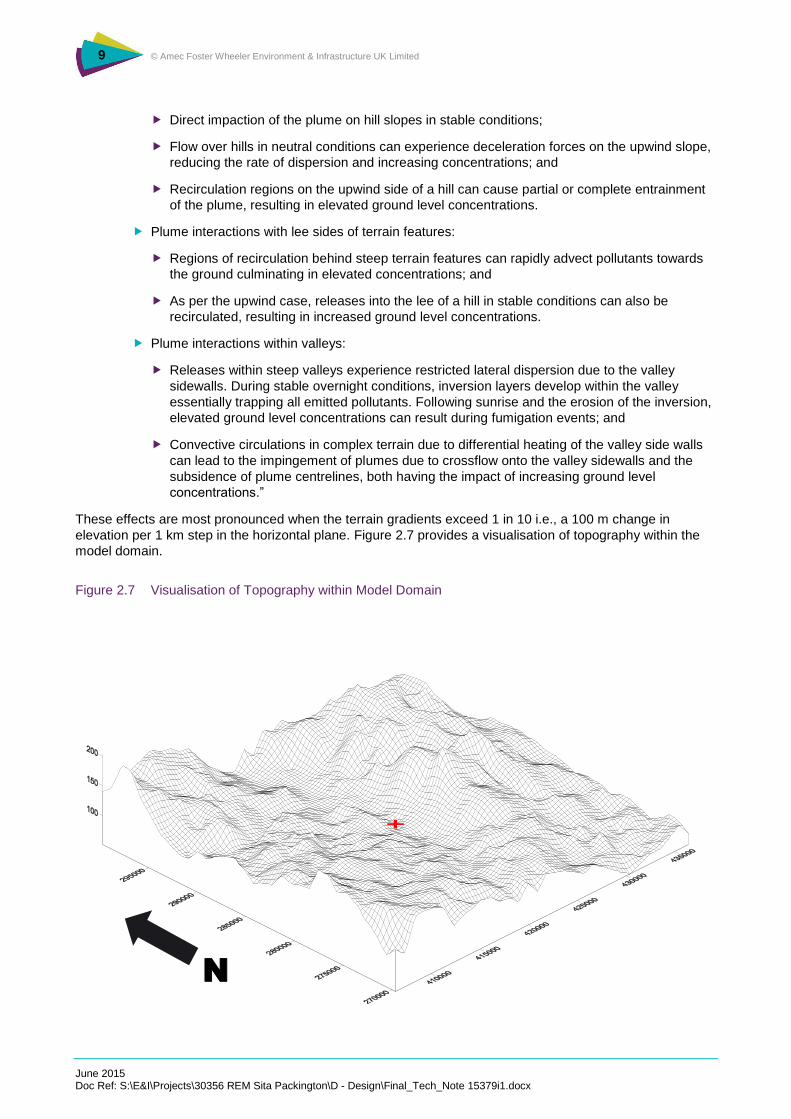
These effects are most pronounced when the terrain gradients exceed 1 in 10 i.e., a 100 m change in
elevation per 1 km step in the horizontal plane. Figure 2.7 provides a visualisation of topography within the
model domain.
Figure 2.7 Visualisation of Topography within Model Domain
N

10 © Amec Foster Wheeler Environment & Infrastructure UK Limited
June 2015 Doc Ref: S:\E&I\Projects\30356 REM Sita Packington\D - Design\Final_Tech_Note 15379i1.docx
2.7 Model Domain and Receptors
Modelled Domain
A 2 km x 2 km Cartesian grid centred on the site, with a receptor resolution of 40 m, was modelled to assess
the impact of atmospheric emissions from the proposed development on local air quality. This resolution is
considered suitable for capturing the maximum process contribution from site emissions.
Human Receptors
The receptors considered were chosen based on places where people may be located, judged in terms of
the likely duration of their exposure to pollutants and proximity to the site. Details of the locations of human
receptors considered in the assessment are given in Table 2.5 and Figure 2.8 below.
Model predictions are made at a height of 1.5 m above ground level, representative of the typical breathing
zone height.
Table 2.5 Modelled Human Receptors
Receptor Name X Y Distance from Site (km)
Packington Hall 422180 283980 1.03
Woodbine Cottage 421411 284860 0.22
House to East 421990 284720 0.59
Common Farm 420025 284883 1.40
Church Farm 421175 284416 0.33
Rectory Cottage 421088 284495 0.36
Beam Ends 421462 284956 0.30
Brook Farm 421555 285058 0.43
Old School House 421842 285149 0.66
North Lodge 421940 284899 0.58
Rockwood Cottage 422013 284722 0.61

11 © Amec Foster Wheeler Environment & Infrastructure UK Limited
June 2015 Doc Ref: S:\E&I\Projects\30356 REM Sita Packington\D - Design\Final_Tech_Note 15379i1.docx
Figure 2.8 Location of Human Receptors
Note: Red symbol marks centre of site
Ecological Receptors
The Environment Agency’s Horizontal Guidance Note H1 requires detailed dispersion modelling to be carried
out based on local receptors. Using this guidance, internationally and nationally-designated ecological sites
(i.e. SPAs, SACs, SSSIs, Ramsar sites and NNRs) within 15 km of the development, and locally-designated
ecological sites within 2 km of the development (e.g. LNRs, ancient woodland etc.) need to be assessed.
The receptors included in the assessment are detailed in Table 2.6 and Figure 2.9.
Table 2.6 Modelled Ecological Receptors
Receptor Name X Y Distance from Site (km)
Coleshill and Bannerly Pools SSSI 421019 285906 1.28
Bickenhill Meadows SSSI 416027 381723 6.14
Berkswell Marsh SSSI 422734 279921 4.93
Hoar Park Wood SSSI 426728 292901 9.80
Whitacre Heath SSSI 420952 292332 7.67
Tilehill Wood SSSI 427597 279214 8.25
River Blythe SSSI 1 421813 284925 0.48

12 © Amec Foster Wheeler Environment & Infrastructure UK Limited
June 2015 Doc Ref: S:\E&I\Projects\30356 REM Sita Packington\D - Design\Final_Tech_Note 15379i1.docx
Receptor Name X Y Distance from Site (km)
River Blythe SSSI 2 421833 284631 0.42
River Blythe SSSI 3 421618 284492 0.27
River Blythe SSSI 4 421484 284402 0.28
Butlers Moors Wood (Potential LWS) 421509 284591 60 m
Figure 2.9 Location of Ecological Receptors

13 © Amec Foster Wheeler Environment & Infrastructure UK Limited
June 2015 Doc Ref: S:\E&I\Projects\30356 REM Sita Packington\D - Design\Final_Tech_Note 15379i1.docx
2.8 Conversion of NO to NO2
Emissions of NOx from combustion processes are predominantly in the form of nitrogen monoxide (NO).
Excess oxygen in the combustion gases and further atmospheric reactions cause the oxidation of NO to
nitrogen dioxide (NO2). NOx chemistry in the lower troposphere is strongly interlinked in a complex chain of
reactions involving Volatile Organic Compounds (VOCs) and Ozone (O3). Two of the key reactions
interlinking NO and NO2 are detailed below:
(R1)
(R2)
Where hv is used to represent a photon of light energy (i.e., sunlight).
Taken together, reactions R1 and R2 produce no net change in O3 concentrations, and NO and NO2 adjust
to establish a near steady state reaction (photo-equilibrium). However, the presence of VOCs and CO in the
atmosphere offer an alternative production route of NO2 for photolysis, allowing O3 concentrations to
increase during the day with a subsequent decrease in the NO2:NOx ratio.
However, at night, the photolysis of NO2 ceases, allowing reaction R2 to promote the production of NO2, at
the expense of O3, with a corresponding increase in the NO2:NOx ratio.
Near to an emission source of NO, the result is a net increase in the rate of reaction R2, suppressing O3
concentrations immediately downwind of the source, and increasing further downwind as the concentrations
of NO begin to stabilise to typical background levels (Gillani and Pliem 1996).
Given the complex nature of NOx chemistry, the Environment Agency’s Air Quality Modelling and
Assessment Unit (AQMAU) has adopted a pragmatic, risk based approach in determining the conversion
rate of NO to NO2 which dispersion model practitioners can use in detailed assessments. AQMAU guidance
advises that the source term should be modelled as NOx (as NO2) and then suggests a tiered approach
when considering ambient NO2:NOX ratios:
Screening Scenario: 50 % and 100 % of the modelled NOx process contributions should be
used for short-term and long-term average concentration, respectively. That is, 50 % of the
predicted NOx concentrations should be assumed to be NO2 for short-term assessments and
100 % of the predicted NOx concentrations should be assumed to be NO2 for long-term
assessments;
Worst Case Scenario: 35 % and 70 % of the modelled NOx process contributions should be
used for short-term and long-term average concentration, respectively. That is, 35 % of the
predicted NOx concentrations should be assumed to be NO2 for short-term assessments and 70
% of the predicted NOx concentrations should be assumed to be NO2 for long-term
assessments; and
Case Specific Scenario: Operators are asked to justify their use of percentages lower than 35 %
for short-term and 70 % for long-term assessments in their application reports.
In line with the AQMAU guidance, this assessment has used the ‘Worst Case Scenario’ approach in
determining the conversion rate of NO to NO2 as a robust assumption.
3. Assessment Criteria
3.1 Criteria Appropriate to the Assessment
Table 3.1 sets out those Air Quality Standards (AQSs) and Environmental Assessment Levels (EALs) that
are relevant to this assessment.

14 © Amec Foster Wheeler Environment & Infrastructure UK Limited
June 2015 Doc Ref: S:\E&I\Projects\30356 REM Sita Packington\D - Design\Final_Tech_Note 15379i1.docx
Table 3.1 Relevant AQSs and EALs
Pollutant AQS/EAL Averaging Period Value (µg m-3)
Nitrogen dioxide (NO2) AQS Annual mean 40
AQS 1-hour mean, not more than 18 exceedences a year (equivalent of 99.79 Percentile)
200
Oxides of nitrogen (NOx) - Ecological Receptors Only
AQS Annual mean 30
EAL Daily mean 75
CO AQS 8-hour mean 10,000
EAL 1-hour mean 30,000
Critical Loads Relevant to the Assessment
The Air Pollution Information System (APIS) provides specific information on the potential effects of nitrogen
deposition on various habitats and species. This information, relevant to habitats of some of the ecological
receptors considered in this assessment, is presented in Table 3.2
Table 3.2 Critical Loads Relevant to this Assessment
Habitat and Species Specific Information
Critical Load (kg N ha-1 yr-1)
Specific Information Concerning Nitrogen Deposition
Temperate and Boreal Forests
10-20 Increased nitrogen deposition in mixed forests increases susceptibility to secondary stresses such as drought and frost, can cause reduced crown growth. Also can reduce the diversity of species due to increased growth rates of more robust plants.
Hay Meadow 20-30 The key concerns are related to changes in species composition following enhanced nitrogen deposition. Indigenous species will have evolved under conditions of low nitrogen availability. Enhanced Nitrogen deposition will favour those species that can increase their growth rates and competitive status e.g. rough grasses such as false brome grass (Brachypodium pinnatum) at the expense of overall species diversity. The overall threat from competition will also depend on the availability of propagules.
Oak Woodland 10-15 Increased nitrogen deposition in Oak forests increases susceptibility to secondary stresses such as drought and frost, can cause reduced crown growth.
4. Background Air Quality
4.1 Continuous Monitoring Data
DEFRA sponsors a network of continuous air quality monitoring stations in the UK; the Automatic Urban and
Rural Network (AURN). However, no such monitoring stations are located within North Warwickshire.

15 © Amec Foster Wheeler Environment & Infrastructure UK Limited
June 2015 Doc Ref: S:\E&I\Projects\30356 REM Sita Packington\D - Design\Final_Tech_Note 15379i1.docx
4.2 Passive Monitoring Data
SITA have been monitoring the local NO2 levels since August 2011 using a local diffusion tube network.
Data is available for the twelve month period prior to the commissioning of the engines at PPP and shows an
average NO2 concentration of 22.8 µg/m3. Results from the 2014 diffusion tube monitoring can be found in
the 2014 Diffusion Tube Survey Results Report1. The location of the local diffusion tubes is shown in Figure
4.1.
Figure 4.1 SITA Operated Diffusion Tubes 2014
4.3 Background Concentrations used in the Assessment
The data for the background concentration used in this assessment are given in Table 4.1 below. Data from
DEFRA’s UK Air Information Resource (UKAIR) using the Pollution Climate Mapping (PCM) model
developed by AEARicardo has been used.
Background mapped concentrations of NOx for each 1km grid square closest to the ecological receptors are
detailed in Table 4.2.
The annual average process contribution is added to the annual average background concentration, to give
a total concentration at each receptor location. This total concentration can then be compared against the
relevant AQS and the likelihood of an exceedance determined.
It is not technically rigorous to add predicted short-term or percentile concentrations to ambient background
concentrations not measured over the same averaging period, since peak contributions from different
sources would not necessarily coincide in time or location. Without hourly ambient background monitoring
data available it is difficult to make an assessment against the achievement or otherwise of the short-term
1 Amec Foster Wheeler (Dec 2014) Packington Diffusion Tube Survey – 2014 Results.

16 © Amec Foster Wheeler Environment & Infrastructure UK Limited
June 2015 Doc Ref: S:\E&I\Projects\30356 REM Sita Packington\D - Design\Final_Tech_Note 15379i1.docx
AQS. For the current assessment, conservative short-term background levels have been derived by applying
a factor of two to the annual mean data as per the recommendation in H1 Annex (f).
Table 4.1 Maximum Short-term and Long-term Ambient Background Concentrations at any Human Receptor
Pollutant Short-term Mean Long-term Mean
NO2 (µg m-3) 45.0 22.5
CO (µg m-3) 764 382
VOCs (µg m-3) - -
NMVOCs1(µg m-3) 0.94 0.47
Note: Benzene data used as a proxy compound
Table 4.2 Long-term Ambient Background concentrations at Designated Ecological Receptors
Receptor NOX Long-Term (Annual) Mean (µg m-3)
River Blythe 14.80
Coleshill and Bannerly Pools, Coleshill Pool Wood 15.86
Whitacre Heath3 20.18
Hoar Park Wood3 13.76
Bickenhill Meadows3 19.72
Berkswell Marsh3 19.71
Tilehill Wood3 19.94
Notes: 1. Values based on UK-AIR estimates to the 2011 base year. 2. Long-term emissions only are assessed at ecological receptors. 3. At a distance of greater than 2km included for information only.
Comparing the nitrogen dioxide background concentrations from UKAIR and the most recent 12-month
diffusion tube data, the UKAIR values are reported as lower than the diffusion tube data. As the diffusion
tube data incorporates emissions from the on-site engines that are already operational, the background
concentration data from UKAIR (industrial component removed) has been used in this assessment. This has
been deemed a robust decision as it means that emissions to air from PPP are accounted for in the
modelled results only.

17 © Amec Foster Wheeler Environment & Infrastructure UK Limited
June 2015 Doc Ref: S:\E&I\Projects\30356 REM Sita Packington\D - Design\Final_Tech_Note 15379i1.docx
5. Results
The following tables details the maximum concentrations at human and ecological receptors for each
pollutant considered in this assessment for long-term and short-term impacts.
5.1 Impacts at Human Receptors
Predicted ground-level concentrations have been derived from atmospheric dispersion modelling of process
emissions from the Packington landfill site. Ground- level concentrations for the human receptors considered
are presented in Tables 5.1 to 5.4 for each of the pollutants modelled.
Table 5.1 NO2 Annual and 1-hour Mean Impacts at Human Receptors
Receptors Annual Mean 99.79%-ile 1-hour mean
AQS (µg m-3)
PC (µg m-3)
PEC (µg m-3)
%PEC of AQS
AQS (µg m-3)
PC (µg m-3)
PEC (µg m-3)
%PEC of AQS
Packington Hall 40 1.07 18.44 46.1% 200 13.73 48.47 24.2%
Woodbine Cottage 40 14.97 33.45 83.6% 200 58.85 95.80 47.9%
House to East 40 1.97 20.44 51.1% 200 22.86 59.81 29.9%
Common Farm 40 0.20 22.72 56.8% 200 5.85 50.89 25.4%
Church Farm 40 4.55 23.02 57.6% 200 31.21 68.16 34.1%
Rectory Cottage 40 3.26 21.73 54.3% 200 27.95 64.89 32.4%
Beam Ends 40 8.84 27.32 68.3% 200 37.39 74.33 37.2%
Brook Farm 40 5.53 24.97 62.4% 200 25.78 64.66 32.3%
Old School House 40 2.75 22.19 55.5% 200 20.06 58.94 29.5%
North Lodge 40 2.71 21.18 53.0% 200 21.68 58.63 29.3%
Rockwood Cottage 40 1.84 18.79 47.0% 200 22.62 56.52 28.3%
Note: AQS = Air Quality Standard; PC = Process Contribution; PEC = Predicted Environmental Concentration (PC + Background)
Long-term and short-term NO2 PCs and PECs at the nearest human receptors are below the AQS and, as
such, no adverse effects on the local human populations are expected.
Figures 5.1 and 5.2 shows the contour plot for annual NO2 and for 1-hour mean NO2 respectively, for the
worst-case year.

18 © Amec Foster Wheeler Environment & Infrastructure UK Limited
June 2015 Doc Ref: S:\E&I\Projects\30356 REM Sita Packington\D - Design\Final_Tech_Note 15379i1.docx
Figure 5.1 Annual Average Concentration of NO2, 2011 meteorological year.
5
100

19 © Amec Foster Wheeler Environment & Infrastructure UK Limited
June 2015 Doc Ref: S:\E&I\Projects\30356 REM Sita Packington\D - Design\Final_Tech_Note 15379i1.docx
Figure 5.2 99.79% percentile 1-hour mean NO2, 2012 meteorological year
20
50

20 © Amec Foster Wheeler Environment & Infrastructure UK Limited
June 2015 Doc Ref: S:\E&I\Projects\30356 REM Sita Packington\D - Design\Final_Tech_Note 15379i1.docx
Table 5.2 CO 1-Hour Mean and 8-Hour Mean Impacts at Human Receptors
Receptors Maximum 1-hour mean Maximum rolling 8-hour mean
EAL (µg m-3)
PC (µg m-3)
PEC (µg m-3)
%PEC of AQS
AQS (µg m-3)
PC (µg m-3)
PEC (µg m-3)
%PEC of AQS
Packington Hall 30,000 722 1424 4.7% 10,000 139 841 8.4%
Woodbine Cottage 30,000 240 942 3.1% 10,000 534 1236 12.4%
House to East 30,000 104 868 2.9% 10,000 142 906 9.1%
Common Farm 30,000 329 1093 3.6% 10,000 40.6 805 8.0%
Church Farm 30,000 298 1062 3.5% 10,000 249 1013 10.1%
Rectory Cottage 30,000 351 1115 3.7% 10,000 215 979 9.8%
Beam Ends 30,000 262 1026 3.4% 10,000 351 1115 11.1%
Brook Farm 30,000 215 979 3.3% 10,000 259 1023 10.2%
Old School House 30,000 257 1021 3.4% 10,000 158 922 9.2%
North Lodge 30,000 235 999 3.3% 10,000 181 945 9.5%
Rockwood Cottage 30,000 125 833 2.8% 10,000 137 845 8.5%
Note: AQS = Air Quality Standard; PC = Process Contribution; PEC = Predicted Environmental Concentration (PC + Background)
Short-term CO PCs and PECs at the nearest human receptors are below the AQS/EAL and, as such, no
adverse effects on the local human receptors are expected.
Table 5.3 VOC Annual and 1-Hour Mean Impacts at Human Receptors
Receptors Maximum 1-Hour Mean Annual Mean
AQO (µg m-3)
PC (µg m-3)
PEC (µg m-3)
%PEC of AQS
AQS (µg m-3)
PC (µg m-3)
PEC (µg m-3)
%PEC of AQS
Packington Hall - 103 - - - 3.48 - -
Woodbine Cottage - 515 - - - 49.5 - -
House to East - 171 - - - 6.34 - -
Common Farm - 74.6 - - - 0.66 - -
Church Farm - 235 - - - 14.5 - -
Rectory Cottage - 212 - - - 10.5 - -
Beam Ends - 250 - - - 29.2 - -
Brook Farm - 187 - - - 18.2 - -
Old School House - 153 - - - 9.02 - -
North Lodge - 183 - - - 8.81 - -
Rockwood Cottage - 168 - - - 5.94 - -
Note: AQS = Air Quality Standard; PC = Process Contribution; PEC = Predicted Environmental Concentration (PC + Background)
There are no AQSs available for either long-term or short-term VOCs – results are presented for information
only.

21 © Amec Foster Wheeler Environment & Infrastructure UK Limited
June 2015 Doc Ref: S:\E&I\Projects\30356 REM Sita Packington\D - Design\Final_Tech_Note 15379i1.docx
Table 5.4 NMVOC Annual Mean Impacts at Human Receptors
Receptors Annual Mean
AQS (µg m-3) PC (µg m-3) PEC (µg m-3) %PEC of AQS
Packington Hall 5 0.25 1.11 22.3%
Woodbine Cottage 5 3.56 4.43 88.5%
House to East 5 0.46 1.39 27.8%
Common Farm 5 0.05 0.98 19.6%
Church Farm 5 1.05 1.98 39.6%
Rectory Cottage 5 0.76 1.69 33.8%
Beam Ends 5 2.11 3.04 60.8%
Brook Farm 5 1.31 2.25 45.0%
Old School House 5 0.65 1.58 31.7%
North Lodge 5 0.63 1.57 31.4%
Rockwood Cottage 5 0.43 1.28 25.7%
Note: AQS = Air Quality Standard; PC = Process Contribution; PEC = Predicted Environmental Concentration (PC + Background)
Long-term NMVOC PCs and PECs at local human receptors are below the AQS, even with the assumption
that all of the emitted NMVOC are a single species (benzene). Therefore no adverse effects on the local
human populations are expected.
5.2 Impacts at Ecological Receptors
Table 5.5 summarises the results of the dispersion modelling assessment for estimating atmospheric
concentrations of NOx at the ecological receptors considered in this assessment.
Table 5.5 NOx Impacts at Ecological Receptors
Receptors Annual Mean Maximum 24-Hour Mean
AQS (µg m-3)
PC (µg m-3)
PEC (µg m-3)
%PEC of AQS
EAL (µg m-3)
PC (µg m-3)
PEC (µg m-3)
%PEC of AQS
Coleshill and Bannerly Pools SSSI
30 1.40 17.26 57.5% 75 16.77 48.5 64.6%
Bickenhall Meadows SSSI
30 0.04 19.76 65.9% 75 0.93 40.4 53.8%
Berkswell Marsh SSSI 30 0.14 19.85 66.2% 75 1.79 41.2 54.9%
Hoar Park Wood SSSI 30 0.06 13.82 46.1% 75 0.89 28.4 37.9%
Whitacre Heath SSSI 30 0.15 20.33 67.8% 75 1.93 42.3 56.4%
Tilehill Wood SSSI 30 0.09 20.02 66.7% 75 3.08 43.0 57.3%
River Blythe SSSI 1 30 5.82 20.62 68.7% 75 33.92 63.5 84.7%
River Blythe SSSI 2 30 4.09 18.90 63.0% 75 38.18 67.8 90.4%

22 © Amec Foster Wheeler Environment & Infrastructure UK Limited
June 2015 Doc Ref: S:\E&I\Projects\30356 REM Sita Packington\D - Design\Final_Tech_Note 15379i1.docx
Receptors Annual Mean Maximum 24-Hour Mean
AQS (µg m-3)
PC (µg m-3)
PEC (µg m-3)
%PEC of AQS
EAL (µg m-3)
PC (µg m-3)
PEC (µg m-3)
%PEC of AQS
River Blythe SSSI 3 30 11.02 25.82 86.1% 75 77.41 107.0 142.7%
River Blythe SSSI 4 30 10.27 25.08 83.6% 75 73.04 102.6 136.9%
Butlers Moors Wood 30 32.76 47.57 158.6% 75 222.49 252.1 336.1%
Denbigh Spinney 30 0.76 16.74 55.8% 75 15.90 47.9 63.8%
Holywell Brook 30 2.56 16.98 56.6% 75 24.65 53.5 71.3%
Siding Wood 30 2.02 16.82 56.1% 75 23.69 53.3 71.1%
Packington Park 30 2.31 16.73 55.8% 75 22.99 51.8 69.1%
Mulliners Rough 30 1.10 16.04 53.5% 75 7.75 37.6 50.2%
Todds Rough 30 2.84 18.70 62.3% 75 21.03 52.7 70.3%
Potential LWS 1 30 2.66 18.52 61.7% 75 26.65 58.4 77.8%
Potential LWS 2 30 2.16 18.02 60.1% 75 21.71 53.4 71.2%
Note: AQS = Air Quality Standard; PC = Process Contribution; PEC = Predicted Environmental Concentration (PC + Background)
Long-term NOx PCs at most of the ecological receptors are below the relevant AQO. The one exception is
the predicted NOx concentration at Butlers Moors Wood. However, looking at the diffusion tube data, results
have consistently shown to be below the AQS of 30 µg m-3.
Furthermore, there is a general understanding that the annual average AQO for vegetation (30 µg m-3 NOx)
does not apply (for compliance purposes) at specified distances from agglomerations (20 km) or other built
up areas, industrial installations, or motorways (5 km). The areas falling within the specified distances have
been referred to as “exclusion zones”. This general understanding is not given explicitly within the Air Quality
Standards Regulations 2010, but can be inferred from the reference to the macro-scale siting of sampling
points (Schedule 1, Part 2 of the Regulations). The locations considered in this assessment lie within 20 km
of the Birmingham conurbation and within 5 km of the M6. Therefore, the AQS for the protection of
vegetation would not apply.
The 24 hour mean NOx PCs at the majority of ecological receptors are below the relevant level. For some
receptors however, there are some exceedences. However the 75 µg m-3 daily mean EAL is derived from the
2000 World Health Organisation (WHO) Air Quality Guidelines for Europe. The WHO state in this document
that, with reference to the daily mean NOx guideline level:
“There is insufficient data to provide these levels with confidence at present.”
Consequently, it is considered that greater emphasis should be placed on achievement with the more
established NOx annual mean AQS.
The River Blythe, as a water body, will not be sensitive to the concentrations of air pollutants, the overriding
issue will be the run-off of pollutants from the surrounding land and discharges into the river.
5.3 Nitrogen Deposition
Table 5.6 contains the results of the deposition analysis for nitrogen.

23 © Amec Foster Wheeler Environment & Infrastructure UK Limited
June 2015 Doc Ref: S:\E&I\Projects\30356 REM Sita Packington\D - Design\Final_Tech_Note 15379i1.docx
Table 5.6 Nitrogen Deposition rates at Ecologically-Designated Sites
Receptor CLmin (kg N ha-1 y-1)
Maximum Predicted PC (kg N ha-1 yr-1)
Background Deposition Rate (kg N ha-1 y-1)
PEDR (kg N ha-1 y-1)
% PC of CLmin
Coleshill and Bannerly Pools SSSI
10 0.14 38.22 38.36 1.4%
Bickenhall Meadows SSSI
20 0.00 20.58 20.58 0.0%
Berkswell Marsh SSSI 10 0.01 50.26 50.27 0.1%
Hoar Park Wood SSSI 10 0.01 45.78 45.79 0.1%
Whitacre Heath SSSI N/A 0.01 13.02 13.03 -
Tilehill Wood SSSI 15 0.01 43.68 43.69 0.1%
River Blythe SSSI 1 N/A 0.59 - - -
River Blythe SSSI 2 N/A 0.41 - - -
River Blythe SSSI 3 N/A 1.11 - - -
River Blythe SSSI 4 N/A 1.04 - - -
Note: CL = Critical Load – the CL selected for each designated site relates to its most N-sensitive habitat (or a similar surrogate) listed on the site citation for which data on Critical Loads are available. PC = process Contribution. PEDR = Predicted Environmental Deposition Rate (= PC + background).
The contribution to the deposition rates from the modelled engine emissions is very small when compared to
the background data, and is unlikely to result in degradation of the ecologically-designated sites; even if the
process contribution was completely eliminated, the ecologically-designated sites would experience
deposition levels significantly higher than the minimum critical load. The model has assumed that all 8
engines operate continuously at maximum output. In reality they will operate to a lesser extent, as the eighth
engine will only be used when another engine is operating at reduced output or is offline for maintenance.
This will mean that the annual average impact will be lower than the modelled predictions.
6. Conclusions
This assessment has used detailed dispersion modelling to undertake an assessment of potential air quality
impacts due to engine emissions to air from Packington Power Plant.
The assessment indicates that predicted environmental concentrations of key pollutants emitted by PPP are
below the appropriate standard/guideline value at all local human receptors. For ecological receptors, long-
term NOx remains below the relevant AQS for all receptors, except for Butlers moors Wood – however
monitoring by passive diffusion tube has shown concentrations to be consistently below the annual AQS. For
those ecological receptors where background deposition rates are already predicted to exceed the critical
load, the impact from the 8 landfill gas engines over the entire range of the designated area is not
considered significant.
The assessment is conservative in terms of the site operational scenario, hours of operation and the year of
meteorological data used to derive maximum concentrations, and therefore the assessment represents the
worst-case emissions scenario.