Numerical Simulation of Dispersion of Emissions from Tema ...
177
Numerical Simulation of Dispersion of Emissions from Tema Oil Refinery in Ghana A dissertation presented to the: Department of NUCLEAR SCIENCES AND APPLICATIONS SCHOOL OF NUCLEAR AND ALLIED SCIENCES COLLEGE OF BASIC AND APPLIED SCIENCES UNIVERSITY OF GHANA by HANNAH ASAMOAH AFFUM (ID: 10174319) BSc (KNUST), 2002 MPhil (UG), 2006 In partial fulfillment of the requirements for the degree of DOCTOR OF PHILOSOPHY in APPLIED NUCLEAR PHYSICS 2015 University of Ghana http://ugspace.ug.edu.gh
Transcript of Numerical Simulation of Dispersion of Emissions from Tema ...

Numerical Simulation of Dispersion ofEmissions from Tema Oil Refinery in Ghana
A dissertation presented to the:
Department of NUCLEAR SCIENCES AND
APPLICATIONS
SCHOOL OF NUCLEAR AND ALLIED SCIENCES
COLLEGE OF BASIC AND APPLIED SCIENCES
UNIVERSITY OF GHANA
by
HANNAH ASAMOAH AFFUM (ID: 10174319)
BSc (KNUST), 2002
MPhil (UG), 2006
In partial fulfillment of the requirements for the
degree of
DOCTOR OF PHILOSOPHY
in
APPLIED NUCLEAR PHYSICS
2015
University of Ghana http://ugspace.ug.edu.gh

Declaration
This thesis is the result of research work undertaken by Hannah Asamaoh
AFFUM in the Department of Nuclear Sciences and Applications, School of
Nuclear and Allied Sciences, University of Ghana, under the supervision of
Prof. Emeritus E.H.K. Akaho (SNAS, UG - Legon, Ghana), Prof. Joseph
J.J. Niemela (ICTP, Trieste, Italy), Prof. Vincenzo Armenio (UT, Trieste,
Italy) and Dr. K. A. Danso (SNAS, UG - Legon, Ghana).
Sign: ...........................................
Hannah Asamaoh Affum(Student)
Sign: ................................................
Prof. Emeritus E.H.K. Akaho(Supervisor)
Sign: ................................................
Prof. J.J. Niemela(Co-Supervisor)
Sign:.................................................
Prof. Vincenzo Armenio(Co-Supervisor)
Sign: ................................................
Dr. K.A. Danso(Co-Supervisor)
ii
University of Ghana http://ugspace.ug.edu.gh

Dedicated to my amazing children, Aseyenedi EsiTamakloe, Woedem Dzidula Tamakloe and
Alesineyram Aku Tamakloe. . .
iii
University of Ghana http://ugspace.ug.edu.gh

Acknowledgements
I would like to express my greatest appreciation to Almighty God without
whom the subsequent happenings would not have been possible.
This PhD project was funded by the International Atomic Energy Agency
(IAEA) through the International Centre for Theoretical Physics (ICTP)
Sandwich Training and Exchange Programme(STEP) in Trieste, Italy. It
is, as such, befitting for these kind sponsors to be the next receipient of my
heart-felt gratitude.
The author would like to express profound thanks to her home principal su-
pervisor, Prof. Emeritus E.H.K. Akaho and home co-supervisor, Dr. K.A.
Danso both of School of Nuclear and Allied Sciences(SNAS), University of
Ghana. Their constant encouragement and strong belief in my ability to
go through this academic exercise is truly appreciated. For agreeing to su-
pervise this thesis and ensuring that I had all that was needed to carry out
this research work successfully, my next thanks go to Prof. J.J. Niemela
and Prof. Vincenzo Armenio of the International Centre for Theoretical
Physics and the University of Trieste respectively. The great exposure ac-
quired through my association is deeply cherished. The intellectual support
from my entire supervisory committee is very much appreciated.
Further appreciation is extended to some technical staff of the Residual
Fluid Catalytic Cracking Unit of the Tema Oil Refinery, Ghana, especially
iv
University of Ghana http://ugspace.ug.edu.gh

the manager Engineer Kwaku Darko, Randy and Priscilla Antwi for will-
ingly commiting to our mini-project of estimating refinery emissions in the
absence of data from flow meters.
I would want to specially thank all the doctoral students and staff of the
fluids laboratory of the University of Trieste whom I came into contact
with and exchanged ideas during my attachment to the laboratory. Ahmad
Fakari and Anna Brunetti deserve special mention for their patience they
displayed in coaching me through the various codes I used at various stages
in this research work. For assisting me to build the Latex code for the
write-up of this thesis and others, I also say a big thanks to Christian
Nuviadenu and Ernest Asare.
A special thanks also goes to Dr. Clement Onime, whom I affectionately call
’Uncle Clement’, Addisu Semie and Grazianno Giancula whose instrumen-
tality is helping with the set-up and running the WRF model can simply
not be overemphasized.
I would also like to thank Jake Doku of the Remote Sensing laboratory of
the University of Ghana for willingly providing elevation and base maps
of my study area. Appreciation is also extended to my colleagues at the
Nuclear Application Centre of the Ghana Atomic Energy Commission for
their assistance. I specifically mention Simon Adzaklo, Alexander Coleman
and Godred Appiah who took turns to pick up my children from school.
v
University of Ghana http://ugspace.ug.edu.gh

Dorotea Calligaro and all staff of the ICTP who in one way or another
helped make life comfortable for me while in ICTP, Trieste are also grate-
fully acknowledged. Spiritual support from members of the ICTP fellowship
and the Chiesa di Evangelica especially Ettore Panizon and family, Tonino
Cuschito and family is very much appreciated.
Last but not least, my sincere gratitude is to all of my family especially my
kind and loving husband Emmanuel for all he sacrificed to care for our chil-
dren, Aseye, Woedem and Alesi, whiles I was on fellowship in Trieste, Italy.
How can I forget the unparalled support from Mawuli, my parents and my
in-laws. I would like to thank them for their love, care and encouragements.
Truly, I could not have done this without you.
All friends who gave support deserve my sincerest thanks, especially my
colleagues who encouraged me during the finalisation of this PhD study.
vi
University of Ghana http://ugspace.ug.edu.gh

Abbreviations
ABL Atmospheric Boundary Layer
AFWA Airforce Weather Agency
AMS Accra Meteorological Station
AQM Air Quality Model
BID Buoyancy-Induced Dispersion
CALMET California Meteorological
CALPOST California Post-Processing
CALPUFF California Puff
CDU Crude Distillation Unit
CTDM Complex Terrain Dispersion Model
DEM Digital Elevation Model
DOAS Differential Optical Absorption Spectrometry
EIPPCB European Integration Pollution Prevention Control Bureau
EPA Environmental Protection Agency
FB Fractional Bias
FSL Forecast Systems Laboratory
GC Gas Chromatography
GFS Global Forecast System
GLCC Global Land Cover Characterization
GM Geometric Mean
GSS Ghana Statistical Service
GV Geometric Variance
vii
University of Ghana http://ugspace.ug.edu.gh

IAEA International Atomic Energy Agency
ICTP International Centre for Theoretical Physics
IOA Index Of Agreement
IS Inertial Sub-layer
ISCST Industrial Source Complex Short-Term
KNUST Kwame Nkrumah University of Science and Technology
LULC Land Use Land Cover
MB Mean Bias
NCAR National Centre for Atmospheric Research
NCEP National Centres for Environmental Prediction
MESOPUFF Mesoscale Puff
NMSE Normalised Mean Square Error
NWP Numerical Weather Prediction
PBL Planetary Boundary Layer
PG Pasquill-Gifford
PM Particulate Matter
PRF Premium Reforming
R Correlation Coefficient
RFCC Residual Fluid Catalytic Cracking
RS Roughness Sub-layer
SNAS School Of Nuclear and Allied Sciences
SRTM Shuttle Radar Topography Mission
TMS Tema Meteorological Station
TOR Tema Oil Refinery
UCL Urban Canopy Layer
UG University of Ghana
UNEP United Nations Environment Programme
USAID United States Agency for International Development
USEPA United States Environmental Protection Agency
viii
University of Ghana http://ugspace.ug.edu.gh

USGS United States Geological Survey
UT University of Trieste
UTM Universal Transverse Mercaptan
VOC Volatile Organic Compound
WRF Weather Research and Forecasting
ix
University of Ghana http://ugspace.ug.edu.gh

Physical Constants
Constant Name Symbol = Constant Value
Acceleration due to gravity g = 9.8 m/s2
Universal Gas Constant R = 8.314 kJK−1mol−1
pi π = 3.14
Von Karman constant κ = 0.41
x
University of Ghana http://ugspace.ug.edu.gh

Symbols
Symbol Name
σ Standard deviation
θ Potential temperature
ξ Virtual source matrix
β Entrainment parameter
ρ Density
Uτ Friction velocity
d Displacement
z Roughness height
u Velocity
C Concentration
V Volume
Q Emission rate
H Mixing depth
rG Ground reflection coefficient
D Molecular diffusivity
S Source/Sink
p Probability distribution function
Z Terrain-following vertical coordinate
ht Terrain height
N Brunt-Vaisala frequency
xi
University of Ghana http://ugspace.ug.edu.gh

k Coefficient of exponential decay
Fr Local Froude number
F Buoyancy
Fm Momentum flux
Ta Ambient Temperature
P Pressure
xii
University of Ghana http://ugspace.ug.edu.gh

Table of Contents
Declaration ii
Acknowledgements iv
Abbreviations vii
Physical Constants x
Symbols xi
List of Tables xvii
List of Figures xviii
Abstract 1
1 General Introduction 3
1.1 Introduction . . . . . . . . . . . . . . . . . . . . . . . . . . . 3
1.2 Background . . . . . . . . . . . . . . . . . . . . . . . . . . . 3
1.3 Problem Statement/Research Gap . . . . . . . . . . . . . . . 5
1.4 Justification and Scope of Work . . . . . . . . . . . . . . . . 6
1.5 Objectives of the Study . . . . . . . . . . . . . . . . . . . . . 8
xiii
University of Ghana http://ugspace.ug.edu.gh

1.6 Dissertation Outline . . . . . . . . . . . . . . . . . . . . . . 8
2 Literature Review 10
2.1 Introduction . . . . . . . . . . . . . . . . . . . . . . . . . . . 10
2.2 Description and Characteristics of the Atmosphere Bound-
ary Layer . . . . . . . . . . . . . . . . . . . . . . . . . . . . 11
2.2.1 Multi-Scale Considerations . . . . . . . . . . . . . . . 13
2.3 Air Quality Models . . . . . . . . . . . . . . . . . . . . . . . 16
2.3.1 Box Models . . . . . . . . . . . . . . . . . . . . . . . 17
2.3.2 Gaussian Models . . . . . . . . . . . . . . . . . . . . 19
2.3.3 Eulerian Models . . . . . . . . . . . . . . . . . . . . 22
2.3.4 Lagrangian Models . . . . . . . . . . . . . . . . . . . 25
2.3.5 Data Requirements for Air Quality Models . . . . . . 27
2.3.5.1 Meteorological data . . . . . . . . . . . . . 27
2.3.5.2 Geophysical Data . . . . . . . . . . . . . . . 28
2.3.5.3 Emission Data . . . . . . . . . . . . . . . . 30
2.3.6 Model Evaluation . . . . . . . . . . . . . . . . . . . . 32
2.4 CALPUFF Modeling System . . . . . . . . . . . . . . . . . . 35
2.4.1 CALMET Diagnostic Meteorological Model . . . . . 36
2.4.2 CALPUFF Model . . . . . . . . . . . . . . . . . . . . 42
2.4.2.1 Dispersion . . . . . . . . . . . . . . . . . . . 43
2.4.2.2 Atmospheric Turbulence Components . . . . 46
2.4.2.3 Buoyancy-Induced Dispersion . . . . . . . . 47
2.4.3 CALPOST . . . . . . . . . . . . . . . . . . . . . . . 49
2.4.4 Weather Research and Forecasting (WRF) Model . . 51
3 Methodology 52
3.1 Introduction . . . . . . . . . . . . . . . . . . . . . . . . . . . 52
3.1.1 The Study Area . . . . . . . . . . . . . . . . . . . . . 53
xiv
University of Ghana http://ugspace.ug.edu.gh
3.1.2 Tema Oil Refinery . . . . . . . . . . . . . . . . . . . 55
3.2 Tema Oil Refinery Emission Estimation . . . . . . . . . . . . 57
3.2.1 Estimation of Flue Stack Gas Rate and Composition 58
3.2.2 Estimation of Flared Gas Composition . . . . . . . . 60
3.2.3 Calculation of Flare and Flue stack Exit Gas Velocities 61
3.2.4 Modelling Period . . . . . . . . . . . . . . . . . . . . 62
3.2.5 Model Set-up . . . . . . . . . . . . . . . . . . . . . . 62
3.2.5.1 CALMET Modelling . . . . . . . . . . . . . 62
3.2.5.2 Geophysical Data Input . . . . . . . . . . . 65
3.2.5.3 CALPUFF modelling . . . . . . . . . . . . 68
3.2.5.4 Model Evaluation . . . . . . . . . . . . . . . 70
4 Results and Discussions 73
4.1 Introduction . . . . . . . . . . . . . . . . . . . . . . . . . . . 73
4.2 Refinery Emissions and Interannual Trends . . . . . . . . . . 73
4.3 Preliminary Dispersion Simulation . . . . . . . . . . . . . . . 76
4.3.1 Spatial Variation of Pollutants . . . . . . . . . . . . . 78
4.4 Validation of the CALPUFF Model . . . . . . . . . . . . . . 82
4.5 Validation of CALMET and WRF
Models . . . . . . . . . . . . . . . . . . . . . . . . . . . . . . 86
4.6 Spatial Distribution of Emissions . . . . . . . . . . . . . . . 105
4.7 Interannual Predicted Concentrations of Emissions at Re-
ceptors . . . . . . . . . . . . . . . . . . . . . . . . . . . . . . 112
4.8 Seasonal Variation of Pollutants . . . . . . . . . . . . . . . . 119
5 Conclusions and Recommendations 127
5.1 Introduction . . . . . . . . . . . . . . . . . . . . . . . . . . . 127
5.1.1 Conclusions . . . . . . . . . . . . . . . . . . . . . . . 128
5.1.2 Recommendations . . . . . . . . . . . . . . . . . . . . 130
xv
University of Ghana http://ugspace.ug.edu.gh

References 133
Appendix A 146
A Estimation of Refinery Emission Rates . . . . . . . . . . . . 146
A.1 Estimation of Flue Stack Gas Rate and Composition 146
A.1.1 Combustion Air Correction to Dry Basis . . 146
A.1.2 Calculation of Flue Gas Rate . . . . . . . . 147
A.1.3 Flue Stack Gas Components . . . . . . . . . 147
A.2 Estimation of Flared Gas Composition . . . . . . . . 150
A.3 Calculation of Flare and Flue Stack Exit Gas Velocities152
xvi
University of Ghana http://ugspace.ug.edu.gh

List of Tables
3.1 Operational Average Flow Parameters of the RFCCU of the
Tema Oil Refinery for 2008 - 2013 . . . . . . . . . . . . . . . 58
3.2 Receptor Locations in the Study Area . . . . . . . . . . . . . 69
4.1 Statistical Performance Indices of the CALPUFF model . . . 85
4.2 Statistical Performance Indices of CALMET and WRF models 87
4.3 Statistical Performance Indices of CALMET and Observa-
tions from the TMS and AMS . . . . . . . . . . . . . . . . . 90
1 Flue Gas Composition . . . . . . . . . . . . . . . . . . . . . 147
2 RFCC Fuel Gas Composition . . . . . . . . . . . . . . . . . 151
3 RFCCU and (Total Refinery) Flare Stack Emission Rates(kg/hr)152
4 RFCCU and (Total Refinery) Flue Stack Emission Rates(kg/hr)152
5 RFCC Point Sources Parameters . . . . . . . . . . . . . . . 152
6 Average Exit Gas Velocities of Point Sources Used for the
Simulations for 2008 - 2013 . . . . . . . . . . . . . . . . . . . 154
xvii
University of Ghana http://ugspace.ug.edu.gh

List of Figures
2.1 Description of the atmospheric layers of the earth (Stull, 2012) 12
2.2 Description of the atmospheric boundary layer (Stull, 2012) 12
2.3 Flow layers over an urban environment (Raupach and Thom,
1981) . . . . . . . . . . . . . . . . . . . . . . . . . . . . . . . 14
2.4 Visualization of a buoyant Gaussian air pollutant dispersion
plume (Holmes and Morawska, 2006) . . . . . . . . . . . . . 19
2.5 A schematic diagram of the program elements in the CAL-
MET/CALPUFF modelling (Scire et al., 2000b) . . . . . . . 50
3.1 Map of Study Area showing the Tema Oil Refinery . . . . . 54
3.2 Nested Computational domains in the WRF simulations . . 64
4.1 Interannual Variation of CO2 Emission Rates from the Tema
Oil Refinery . . . . . . . . . . . . . . . . . . . . . . . . . . . 74
4.2 Interannual Variation of VOCs Emission Rates from the
Tema Oil Refinery . . . . . . . . . . . . . . . . . . . . . . . 74
4.3 Interannual Variation of PM2.5 Emission Rates from the
Tema Oil Refinery . . . . . . . . . . . . . . . . . . . . . . . 75
4.4 Interannual Variation of SO2 Emission Rates from the Tema
Oil Refinery . . . . . . . . . . . . . . . . . . . . . . . . . . . 75
4.5 Interannual Variation of NO2 Emission Rates from the Tema
Oil Refinery . . . . . . . . . . . . . . . . . . . . . . . . . . . 76
xviii
University of Ghana http://ugspace.ug.edu.gh

4.6 Terrain Map of the Study area showing receptor locations
and the Refinery (red square) . . . . . . . . . . . . . . . . . 77
4.7 LandUse Map of the Study Area . . . . . . . . . . . . . . . . 77
4.8 Predicted Daily Average Concentrations of SO2, NO2 and
PM2.5 at northern receptors in the Study area . . . . . . . . 79
4.9 Predicted Daily Average Concentrations of SO2, NO2 and
PM2.5 at north eastern receptors in the Study area . . . . . . 79
4.10 Predicted Daily Average Concentrations of SO2, NO2 and
PM2.5 at south eastern receptors in the Study area . . . . . 80
4.11 Predicted Daily Average Concentrations of SO2, NO2 and
PM2.5 at south western receptors in the Study area . . . . . 80
4.12 Predicted Daily Average Concentrations of SO2, NO2 and
PM2.5 at northern western receptors in the Study area . . . 81
4.13 Wind Rose Depicting Surface Winds in Tema for 2008 . . . 82
4.14 Plots of measured and modelled SO2 Concentrations . . . . 83
4.15 Plots of measured and modelled NO2 Concentrations . . . . 83
4.16 Plots of Observed and Modelled Wind Speeds . . . . . . . . 86
4.17 Plots of Observed and Modelled Wind Direction . . . . . . . 87
4.18 Wind Rose Depicting CALMET Surface Winds . . . . . . . 88
4.19 Wind Rose Depicting WRF Surface Winds . . . . . . . . . . 89
4.20 Plots of Modelled and Observed(AMS) Surface Wind direc-
tion for 2008 . . . . . . . . . . . . . . . . . . . . . . . . . . . 91
4.21 Plots of Modelled and Observed(AMS) Surface Wind direc-
tion for 2009 . . . . . . . . . . . . . . . . . . . . . . . . . . . 92
4.22 Plots of Modelled and Observed(AMS) Surface Wind direc-
tion for 2010 . . . . . . . . . . . . . . . . . . . . . . . . . . . 92
4.23 Plots of Modelled and observed(AMS) Surface Wind direc-
tion for 2011 . . . . . . . . . . . . . . . . . . . . . . . . . . . 93
xix
University of Ghana http://ugspace.ug.edu.gh

4.24 Plots of Modelled and observed(AMS) Surface Wind direc-
tion for 2012 . . . . . . . . . . . . . . . . . . . . . . . . . . . 93
4.25 Plots of Modelled and observed(AMS) Surface Wind direc-
tion for 2013 . . . . . . . . . . . . . . . . . . . . . . . . . . . 94
4.26 Plots of Modelled and Observed(TMS) Surface Wind direc-
tion for 2008 . . . . . . . . . . . . . . . . . . . . . . . . . . . 94
4.27 Plots of Modelled and Observed(TMS) Surface Wind direc-
tion for 2009 . . . . . . . . . . . . . . . . . . . . . . . . . . . 95
4.28 Plots of Modelled and Observed(TMS) Surface Wind direc-
tion for 2010 . . . . . . . . . . . . . . . . . . . . . . . . . . . 95
4.29 Plots of Modelled and observed(TMS) Surface Wind direc-
tion for 2011 . . . . . . . . . . . . . . . . . . . . . . . . . . . 96
4.30 Plots of Modelled and observed(TMS) Surface Wind direc-
tion for 2012 . . . . . . . . . . . . . . . . . . . . . . . . . . . 96
4.31 Plots of Modelled and observed(TMS) Surface Wind direc-
tion for 2013 . . . . . . . . . . . . . . . . . . . . . . . . . . . 97
4.32 Plots of Modelled and Observed(AMS) Surface Wind Speed
for 2008 . . . . . . . . . . . . . . . . . . . . . . . . . . . . . 98
4.33 Plots of Modelled and Observed(AMS) Surface Wind Speed
for 2009 . . . . . . . . . . . . . . . . . . . . . . . . . . . . . 99
4.34 Plots of Modelled and Observed(AMS) Surface Wind Speed
for 2010 . . . . . . . . . . . . . . . . . . . . . . . . . . . . . 99
4.35 Plots of Modelled and Observed(AMS) Surface Wind Speed
for 2011 . . . . . . . . . . . . . . . . . . . . . . . . . . . . . 100
4.36 Plots of Modelled and Observed(AMS) Surface Wind Speed
for 2012 . . . . . . . . . . . . . . . . . . . . . . . . . . . . . 100
4.37 Plots of Modelled and Observed(AMS) Surface Wind Speed
for 2013 . . . . . . . . . . . . . . . . . . . . . . . . . . . . . 101
xx
University of Ghana http://ugspace.ug.edu.gh

4.38 Plots of Modelled and Observed(TMS) Surface Wind Speed
for 2008 . . . . . . . . . . . . . . . . . . . . . . . . . . . . . 102
4.39 Plots of Modelled and Observed(TMS) Surface Wind Speed
for 2009 . . . . . . . . . . . . . . . . . . . . . . . . . . . . . 103
4.40 Plots of Modelled and Observed(TMS) Surface Wind Speed
for 2010 . . . . . . . . . . . . . . . . . . . . . . . . . . . . . 103
4.41 Plots of Modelled and Observed(TMS) Surface Wind Speed
for 2011 . . . . . . . . . . . . . . . . . . . . . . . . . . . . . 104
4.42 Plots of Modelled and Observed(TMS) Surface Wind Speed
for 2012 . . . . . . . . . . . . . . . . . . . . . . . . . . . . . 104
4.43 Plots of Modelled and Observed(TMS) Surface Wind Speed
for 2013 . . . . . . . . . . . . . . . . . . . . . . . . . . . . . 105
4.44 2008 Annual Average Concentration contours of SO2 in the
Study Area . . . . . . . . . . . . . . . . . . . . . . . . . . . 106
4.45 2008 Annual Average Concentration contours of NO2 in the
Study Area . . . . . . . . . . . . . . . . . . . . . . . . . . . 107
4.46 2008 Annual Average Concentration contours of PM2.5 in the
Study Area . . . . . . . . . . . . . . . . . . . . . . . . . . . 108
4.47 2009 Annual Average Concentration contours of SO2 in the
Study Area . . . . . . . . . . . . . . . . . . . . . . . . . . . 109
4.66 Wind Rose Depicting 2013 Surface Winds in the Study area 109
4.48 2009 Annual Average Concentration contours of NO2 in the
Study Area . . . . . . . . . . . . . . . . . . . . . . . . . . . 110
4.49 2009 Annual Average Concentration contours of PM2.5 in the
Study Area . . . . . . . . . . . . . . . . . . . . . . . . . . . 110
4.50 Wind Rose Depicting 2009 Surface Winds in the Study area 111
4.51 2010 Annual Average Concentration contours of SO2 in the
Study Area . . . . . . . . . . . . . . . . . . . . . . . . . . . 112
xxi
University of Ghana http://ugspace.ug.edu.gh

4.52 2010 Annual Average Concentration contours of NO2 in the
Study Area . . . . . . . . . . . . . . . . . . . . . . . . . . . 113
4.53 2010 Annual Average Concentration contours of PM2.5 in the
Study Area . . . . . . . . . . . . . . . . . . . . . . . . . . . 113
4.54 Wind Rose Depicting 2010 Surface Winds in the Study area 114
4.55 2011 Annual Average Concentration contours of SO2 in the
Study Area . . . . . . . . . . . . . . . . . . . . . . . . . . . 115
4.56 2011 Annual Average Concentration contours of NO2 in the
Study Area . . . . . . . . . . . . . . . . . . . . . . . . . . . 115
4.57 2011 Annual Average Concentration contours of PM2.5 in the
Study Area . . . . . . . . . . . . . . . . . . . . . . . . . . . 116
4.58 Wind Rose Depicting 2011 Surface Winds in the Study area 117
4.59 2012 Annual Average Concentration contours of SO2 in the
Study Area . . . . . . . . . . . . . . . . . . . . . . . . . . . 118
4.60 2012 Annual Average Concentration contours of NO2 in the
Study Area . . . . . . . . . . . . . . . . . . . . . . . . . . . 118
4.61 2012 Annual Average Concentration contours of PM2.5 in the
Study Area . . . . . . . . . . . . . . . . . . . . . . . . . . . 119
4.62 Wind Rose Depicting 2012 Surface Winds in the Study area 120
4.63 2013 Annual Average Concentration contours of SO2 in the
Study Area . . . . . . . . . . . . . . . . . . . . . . . . . . . 121
4.64 2013 Annual Average Concentration contours of NO2 in the
Study Area . . . . . . . . . . . . . . . . . . . . . . . . . . . 121
4.67 Daily Average SO2 Concentrations at various receptors . . . 122
4.68 Daily Average NO2 Concentrations at various receptors . . . 122
4.69 Daily Average PM2.5 Concentration at various receptors . . . 123
4.70 2013 Monthly Average concentrations of pollutants at Tema
Steelworks . . . . . . . . . . . . . . . . . . . . . . . . . . . . 124
xxii
University of Ghana http://ugspace.ug.edu.gh

4.71 2013 Monthly Average concentrations of pollutants at Tema
Comm. 25 . . . . . . . . . . . . . . . . . . . . . . . . . . . . 124
4.72 2013 Monthly Average concentrations of pollutants at Kpone 125
4.73 2013 Monthly Average concentrations of pollutants at Tema
Gen. Hosp . . . . . . . . . . . . . . . . . . . . . . . . . . . . 125
4.74 Variation of Ambient Temperature around the refinery . . . 126
xxiii
University of Ghana http://ugspace.ug.edu.gh

Abstract
The petrochemical industry is a major contributor of industrial air pol-
lutants which are known to have dire consequences on human health and
the environment, neccesitating research into their dispersion and transport.
The objective of the study, therefore, is to simulate the dispersion and trans-
port of pollutants emitted during the processing of crude oil by the Tema
Oil Refinery in the Greater Accra region of Ghana using the California
Puff (CALPUFF) modeling system. This thesis couples the Weather Re-
search and forecasting Model (WRF) with the non-steady state California
Puff(CALPUFF) modelling system to simulate the dispersion and trans-
port of emissions from the refinery in a coastal urban/industrial area in
Ghana. The mass balance approah was employed to estimate the refinery
emission rates which were used as input for the dispersion model. Emission
rates of five species were estimated - SO2, NO2, PM2.5, CO2 and VOCs.
The transport and dispersion of SO2, NO2 and PM2.5 were modelled over
the period between 2008 - 2013 and their impact on 38 identified receptors
investigated. Simulation results showed that the radius of impact of the
emissions is approximately 10 km. As a result of the prevailing predomi-
nant south-westerly winds in the study area, concentrations of emissions at
receptors located upwind of the emission source were found to be higher as
the winds carried the pollutant clouds in their direction. Conversely, south
and south-western receptors, relative to the refinery, on the other hand,
1
University of Ghana http://ugspace.ug.edu.gh

Abstract 2
were minimally impacted. Concentrations of SO2 and NO2 at 2 out of the
38 receptors exceeded the regulatory limit of the World Health Organisa-
tion and Ghana’s Environmental Protection Agency. It can be concluded,
therefore, that SO2 and NO2 emissions from the refinery do not pose any
danger to the larger population and the general environment nearby. PM2.5
levels at 36 receptors however exceeded the WHO guideline value leading
to the conclusion that the refinery operations could pose some dangers
to the environment regarding PM2.5. The dispersion model results were
compared with measurements at the same location in order to validate
the model. Similarly, observations from two meteorological stations were
compared with results from the meteorological model. The performance
evaluation, with the aid of statistical measures revealed that the models’
performance were acceptable.
University of Ghana http://ugspace.ug.edu.gh

Chapter 1
General Introduction
1.1 Introduction
This thesis deals with the modeling and simulation of the long-range trans-
port and dispersion of refinery emissions over a defined study area. The
first chapter of the dissertation provides a brief background of the thesis
subject area, gives the problem statement, the justification and scope of
this research and finally outlines the objectives of the study.
1.2 Background
All life forms on this planet depend on clean air. Air quality not only affects
human health but also components of environment such as water, soil and
forests which are the vital resources for human development. A major
3
University of Ghana http://ugspace.ug.edu.gh

Chapter 1. General Introduction 4
threat to the availability of clean air is urbanisation. Urbanization is a
process of relative growth in a country's urban population accompanied by
an even faster increase in the economic, political and cultural importance of
cities relative to rural areas. As an integral part of economic development,
urbanisation brings in its wake a number of challenges including the increase
in urban population, industrial activities, high rise buildings and vehicular
movement. All these activities contribute to air pollution (de Leeuw et al.,
2001, Fenger, 1999).
Exposure to such air pollutants may adversely affect human health. Short
term exposure to peak levels of particulate matter has been strongly associ-
ated with adverse respiratory health impacts (e.g., respiratory diseases such
as asthma and pulmonary function insufficiency) (Brunekreef and Holgate,
2002, Guilbert et al., 2003, Hansard et al., 2011). Furthermore, particulate
matter, hereafter referred to as PM, is known to degrade atmospheric visi-
bility. High concentrations of sulphur dioxide, SO2, which are also emitted
from power plants, industrial processes and during the combustion of fossil
fuels, can aggravate respiratory diseases as well as cause problems such as
acid rain and damaged vegetation in the form of foliar necrosis (Khamsi-
mak et al., 2012). Additionally, air pollution is not only a human health
problem: its effects on ecosystems and materials are well identified and
documented (Fowler et al., 2009). Economic costs can also be associated
with poor air quality as well as political/governmental measures taken to
University of Ghana http://ugspace.ug.edu.gh

Chapter 1. General Introduction 5
prevent or reduce pollution (Muller and Mendelsohn, 2007).
1.3 Problem Statement/Research Gap
The USEPA, USAID and UNEP as far as July 2004, selected Accra, Ghana
as one of two cities in Africa to benefit from an Air Quality Monitoring Ca-
pacity Building Project with the aim to build and establish local capacity
on air quality monitoring that will provide policy-makers with information
on the air quality in Accra and its impacts on health. Subsequent to this,
the EPA, Ghana replicated the project in a few more cities in Ghana with
emphasis on PM measurements. SO2 and NO2 emissions from vehicular
traffic have also been monitored in parts of Accra. Apart from the EPA’s
efforts, similar monitoring activities have been carried out, especially within
the Accra metropolis, by students and groups of scientists for different pe-
riods of time largely on heavy metals. For example, Arku et al. (2008)
conducted a study for an initial assessment of the levels and spatial and/or
temporal patterns of multiple pollutants in the ambient air in two low-
income neighborhoods in Accra, Ghana over a 3-week period while Ofosu
et al. (2012) characterized fine particulate sources at Ashaiman in Greater
Accra, Ghana. Others include the assessment of particulate matter and
heavy metals along major highways and in mining areas (Affum et al., 2008,
Bansah and Amegbey, 2012, Safo-Adu et al., 2014). Quite recently, Sackey
University of Ghana http://ugspace.ug.edu.gh

Chapter 1. General Introduction 6
(2012) employed Differential Optical Absorption Spectroscopy (DOAS) in
the measurement of atmospheric constituents as a result of combustion,
vehicular emissions and industrial activities around the Tema Oil refin-
ery. There is, however, limited or no information about the behaviour and
spread of these pollutants from specific sources in the atmosphere within
the country. This is because none of the research works focussed on a spe-
cific industry, its air emissions and rates and the transport of the emissions
within its catchment area. A gap therefore exists in this area of research
which thesis seeks to fill through atmospheric dispersion modelling.
1.4 Justification and Scope of Work
The simplest technique for evaluating patterns of local-scale urban air pol-
lution concentration involves the interpolation of ambient concentrations
from existing monitoring networks (Ferretti et al., 2008, Perez Ballesta
et al., 2008). However, the measured data from these stations or study
areas are not necessarily representative of areas beyond their immediate
vicinity. This is because concentrations of pollutants in urban areas may
greatly vary on spatial scales that range from tens to hundreds of metres.
Moreover, the establishment and operation of monitoring stations are ex-
pensive and can only be expected to be established in few locations. At the
same time, the temporal behaviour of primary and secondary pollutants
University of Ghana http://ugspace.ug.edu.gh

Chapter 1. General Introduction 7
changes considerably between day and night due to solar radiation, so that
daily average measurements become unsatisfactory in determining or ex-
plaining high pollution episodes. In such instances, air pollution dispersion
models become necessary.
Dispersion modelling studies, in combination with air quality monitoring,
are essential and complementary tools for long and short term air pollu-
tion control strategies in effective air quality management. Air quality and
dispersion models become valid instruments for environmental managers
in many activities, such as setting emission control regulations, testing the
compliance of actual pollution levels, predicting the impact of new facili-
ties on human health, selecting the best location for monitoring stations
and assessing the impact of different emissions scenarios on selected loca-
tions (Puliafito et al., 2011). Modelling studies are crucial as they provide
useful data on the dynamics of pollutant dispersion and transport among
others, which feed into the formulation of environmental policies as well
as management processes. Furthermore, they improve the limitations of
monitoring networks by providing predictions of the temporal and spatial
distribution of actual pollution levels. The focus of this thesis, therefore,
is to utilize air quality modeling to fill the gap that presently exists in the
area of air pollution studies within the country.
Due to the significant contribution of petroleum refineries to air pollution,
this thesis investigates the long-range transport of emissions from Ghana’s
University of Ghana http://ugspace.ug.edu.gh
Chapter 1. General Introduction 8
only refinery, Tema Oil Refinery, using numerical models.
1.5 Objectives of the Study
The main objective of the study is to simulate the dispersion and transport
of pollutants emitted during the processing of crude oil by the Tema Oil
Refinery, hereafter referred to as TOR, in the Greater Accra region of
Ghana using the California Puff (CALPUFF) modeling system. This will
be achieved through the following specific objectives:
1. To estimate the emission rates of CO2, SO2, NO2, volatile organic
compounds (VOCs) and PM2.5 during refinery operations at the TOR.
2. To simulate the transport and dispersion of the emissions and
3. To access the impact of meteorological conditions on the dispersion
of the emissions.
1.6 Dissertation Outline
This thesis is organized as follows: The first chapter of the dissertation
provides a brief background of the thesis area, gives the problem statement,
the justification and scope of this research and finally outlines the objectives
of the study.
University of Ghana http://ugspace.ug.edu.gh

Chapter 1. General Introduction 9
In Chapter 2, a literature review of the subject area is presented. Emissions
and their sources are discussed briefly after which an overview of some air
quality models and their applications as well as their strengths and limi-
tations are presented. A detailed description of the CALPUFF/CALMET
models used for the simulation is also included in this chapter. A short
presentation of the prognostic mesoscale WRF model used to simulate the
wind fields is also provided.
In Chapter 3, the methodology for the simulation of the pollutants disper-
sion in the study area is presented. First of all, the methodology for the
estimation of pollutants from the refinery is presented. This is followed by
a description of the various data resources used for the simulation. The val-
idation methodology of all simulation results is also described using some
statistical tools.
A thorough discussion of the research results and its contribution to the
wider literature are presented in Chapter 4.
Finally in Chapter 5, conclusions and recommendations are presented. The
limitations and challenges of the work are also discussed and future work
outlined.
University of Ghana http://ugspace.ug.edu.gh

Chapter 2
Literature Review
2.1 Introduction
This Chapter presents some general concepts and theoretical frameworks
in air pollution studies. Various air quality models in literature are also
reviewed. A detailed description of the numerical models used for the sim-
ulations in this thesis, namely the California Puff (CALPUFF) modelling
system and WRF, a description of the study area and the emission source
of interest, TOR are also presented. The equations forming the basis of the
models are presented as well as an overview of the Residual Fluid Catalytic
Cracking (RFCC) process in petroleum refining at the TOR.
10
University of Ghana http://ugspace.ug.edu.gh

Chapter 2. Literature Review 11
2.2 Description and Characteristics of the
Atmosphere Boundary Layer
A discussion of the layers in the earth’s atmosphere is needed to better
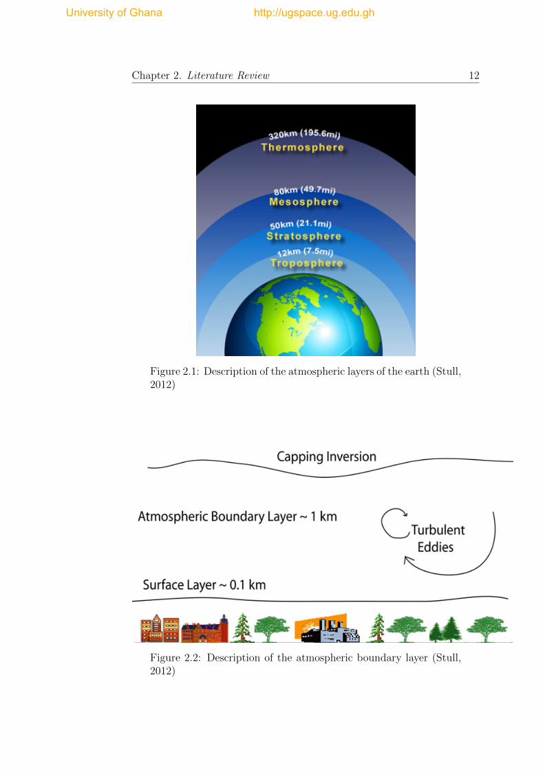
understand where air pollution dispersion takes place. The main layers of
the earth’s atmosphere, from the surface of the ground upwards, as shown
in Fig.2.1 are the troposphere (0 to 15 km), the stratosphere (15 to 50 km),
the mesosphere (50 to 85 km), the thermosphere and others (more than
85 km). The lowest part of the troposphere is the Atmospheric Boundary
Layer (ABL) or Planetary Boundary Layer (PBL) which extends from the
earth’s surface to about 1.5 to 2.0 km in height (Stull, 2012). The ABL is
made up of the mixing layer, capped by the inversion layer, and is separated
by a change in temperature behaviour in the vertical direction as shown in
Fig.2.2.
Human activity is generally confined to the ABL such that pollutant sources
are created in this area. Thus the challenge of modeling pollutant dispersion
is understanding how materials are mixed by turbulence and transported
from the release point to larger scales (Fernando, 2010). Fundamentally,
it is characterized by a large shearing stress resulting from momentum
transfer at the surface. The exact structure of the ABL is determined by
both the character of the surface and the geostrophic winds aloft driving
it. Geostrophic winds are a global scale phenomena derived from a basic
University of Ghana http://ugspace.ug.edu.gh
Chapter 2. Literature Review 12
Figure 2.1: Description of the atmospheric layers of the earth (Stull,2012)
Figure 2.2: Description of the atmospheric boundary layer (Stull,2012)
University of Ghana http://ugspace.ug.edu.gh

Chapter 2. Literature Review 13
balance between pressure and Coriolis force which is the apparent deflection
of objects moving in a straight path relative to the earth’s surface. For
conditions of neutral stability, the depth of the ABL can vary from several
hundred meters to over a thousand meters depending on the speed of the
geostrophic wind (Pasquill and Smith, 1983). Neutral stability is often
a fair assumption for the ABL over urban areas, especially at night, as
physical factors like surface drag force due to roughness and heat-storage
promote these conditions (Britter and Hanna, 2003).
2.2.1 Multi-Scale Considerations
To do a better analysis of the fluid dynamics of the lower atmosphere,
it is helpful to recognize the multi-scale phenomena present. The global
processes that drive regional weather conditions and atmospheric bound-
ary layer formation will not be the focus of this Thesis. Instead, flow
phenomena affecting dispersion at the cities/neighbourhood scale will be
considered.
At the city/neighborhood scale, the ABL is further divided into regions
describing the impact of the urban environment. The effect of individual
buildings on the flow at this scale is conceptualized as flow over a series of
roughness elements such as buildings, trees and hills. Closest to the ground,
the buildings are said to reside in the canopy layer which extends to the
University of Ghana http://ugspace.ug.edu.gh

Chapter 2. Literature Review 14
height of the tallest building. After the canopy layer is the Roughness
Sublayer (RS) followed by the Inertial Sublayer (IS) as seen in Fig.2.3.
Figure 2.3: Flow layers over an urban environment (Raupach andThom, 1981)
The RS, as defined by Raupach and Thom (1981), is the region over which
mean flow and turbulence properties depend on the specific details of the
roughness (i.e. the buildings) itself. As such, the exact definition of its
extent varies throughout the literature. The lower boundary is sometimes
considered to be the mean building height and in other cases the zero-plane
displacement, d, which is defined based on a logarithmic velocity profile
(Rotach, 1994). The upper boundary of the RS occurs when the horizontal
variation in flow and turbulence parameters caused by the canopy subsides,
though exact applications of this concept vary.
University of Ghana http://ugspace.ug.edu.gh

Chapter 2. Literature Review 15
The IS, is by definition, a layer of constant shear stress where Monin-
Obukhov similarity arguments apply (Monin and Obukhov, 1954). For
stable conditions over a rough surface, this leads to a logarithmic velocity
profile of the form as depicted by Eqn.( 2.1):
u(z) =uτκln
(z − dz0
)(2.1)
where
uτ is the friction velocity,
z0 is the characteristic roughness height
d is the previously mentioned zero-plane displacement and
κ is the Von Karman constant.
Jackson (1981) showed that d represents the level at which the mean surface
drag acts, while z0 is a measure of the magnitude of that drag. Values
of z0 and d have been tabulated from experimental data for a range of
surfaces from croplands and forests to concrete roads and towns (Wieringa
et al., 2001). The range reported for any one given surface type illustrates
the approximate nature with which z0 and d are often interpreted. The
complexity in determining a precise value stems from the fact that z0 and
d depend not only on the specific geometrical properties of the roughness
elements, but also on the flow conditions. Nevertheless, the logarithmic
University of Ghana http://ugspace.ug.edu.gh

Chapter 2. Literature Review 16
velocity profile is typically used not only in the range where it is strictly
valid, but is extended into the roughness sublayer. Macdonald (2000) noted
that this is done out of a lack of information about flow within the canopy
and is generally an acceptable approximation for studies of larger, elevated
plumes.
2.3 Air Quality Models
In basic applications of air quality models, the processes of air pollution
transport are considered as a distributed parameter system, which is gov-
erned by a set of transport equations, along with respective boundary and
initial conditions. The exact form and structure of a model usually depend
on its practical application, type of the polluting compounds considered
and the scale of modelling. A model usually takes into account the input
data (emission field and meteorological data) as well as the main physical
and chemical processes which determine the transport in the atmosphere
and transformations of air pollution components (Holnicki, 2011). The
characteristics of each specific problem will define the physical and chemi-
cal processes involved, and consequently, the best model to use. The main
criteria for choosing appropriate software are:
1. The dimension of the area under study
University of Ghana http://ugspace.ug.edu.gh

Chapter 2. Literature Review 17
2. The number of pollution sources
3. The chemical species involved and
4. The time scale of the episode.
The spatial and temporal scales of the environmental impact of air pollu-
tion are correlated with the lifetime of a pollutant. Thus, depending on the
analysis scale, there are respective categories of modelling: local, regional
and global. Regarding the practical application and the scale of modelling,
the most common types (implementations) of air pollution models are dis-
cussed in the following section.
2.3.1 Box Models
Box models are derived by simply applying a control volume-based mass
conservation approach to determining concentration levels in a domain of
interest. This leads to a uniform prediction of concentration without pro-
viding information about spatial variation in concentration within the box
(Holmes and Morawska, 2006). The domain is treated as a box into which
pollutants are emitted and undergo chemical and physical processes. They
require the input of simple meteorology and emissions and the movement
of pollutants in and out of the box is allowed. The model also assumes
that the incoming pollution is instantaneously mixed with the surrounding
University of Ghana http://ugspace.ug.edu.gh

Chapter 2. Literature Review 18
air, creating a homogeneous concentration throughout the airshed (Venka-
tram, 1978). The mass conservation constraint permits the construction of
a mass balance equation of the form as shown in Eqn.(2.2):
dcV
dt= QA+ ucinWH − ucWH (2.2)
where
V is the volume described by the box,
c is the homogeneous species concentration within the airshed,
cin is the species concentration entering the airshed,
Q is the emission rate per unit area of sources within the box,
u is the average wind speed normal to the box,
A is the horizontal area of the box (L × W ),
W is the width of the box and
H is the mixing depth.
Integrating Eqn.( 2.2) provides a steady state estimation of species concen-
tration (Venkatram, 1978) assuming the dynamics of the mixing depth to
be quasi-stationary and the source emissions to be constant. In the case of
reactive species, the chemical reaction dynamics can be incorporated into
the mass balance equation as well as wet and dry deposition effects.
University of Ghana http://ugspace.ug.edu.gh

Chapter 2. Literature Review 19
It is incapable of imparting any spatial information regarding the dispersive
nature of a pollutant. This precludes the box model approach from a
significant proportion of air quality modelling applications. Nevertheless,
the method is computationally fast and is capable of providing satisfactory
predictions, particularly for scenarios where detailed information on the
domain and meteorological conditions is unavailable.
2.3.2 Gaussian Models
The Gaussian model forms the basis for the majority of air pollution mod-
els, and is the most well known and documented approach. The model
presupposes that the dispersion associated with the polluting species can
be described by a modified Gaussian or normal distribution curve as shown
in Fig.2.4.
Figure 2.4: Visualization of a buoyant Gaussian air pollutant dis-persion plume (Holmes and Morawska, 2006)
University of Ghana http://ugspace.ug.edu.gh

Chapter 2. Literature Review 20
A three-dimensional axis system is employed to provide a downwind, cross-
wind and vertical resolution. The species concentration is defined as being
proportional to the emission rate of the source, diluted by the wind veloc-
ity at the source of emission. The dispersion behaviour of a pollutant is
determined by the standard deviations associated with the Gaussian distri-
bution function. These standard deviations which are related to the turbu-
lent diffusivities are typically functions of atmospheric stability, localised
turbulence and distance downwind from the source. Since the turbulent
diffusivity is unknown, however, the deviations are parameterized based
on experimental measurements and observations. The parametrization is
typically a function of conditions like atmospheric stability (Holmes and
Morawska, 2006). The model is usually aligned so that the downwind axis
corresponds to the direction of the prevailing wind (Collett and Oduyemi,
1997). The model equation is derived from basic considerations of the dif-
fusion of gaseous matter in three-dimensional space as shown in Eqn.(2.3):
C =Q
2πuσyσzexp
(−y2
2σ2y
)[exp
(−(h− z)2
2σ2y
)+ rGexp
(−(h+ z)2
2σ2y
)](2.3)
where
C is the species concentration at a location (x, y, z),
Q is the source emission rate,
University of Ghana http://ugspace.ug.edu.gh

Chapter 2. Literature Review 21
u is the average wind speed normal to the box,
σy is the standard deviation of the horizontal crosswind distribution of the
plume concentration and is a function of the downwind distance x,
σz is the standard deviation of the vertical crosswind distribution of the
plume concentration and is a function of the crosswind distance z,
h is the effective source height to which the plume has risen,
rG is the ground reflection coefficient where 0≤ rG≥ 1,
y is the crosswind distance and
z is the receptor height above ground.
The effective source height (h) or plume rise is the height to which an
emission will initially rise as a result of thermal buoyancy and vertical mo-
mentum. The upward movement of the plume is retarded on mixing with
ambient air reaching an equilibrium point when the internal energy of the
plume is equal to that of the surrounding atmosphere. A review of vari-
ous semi-empirical methods for the estimation of plume rise can be found
in Zannetti (2013). Several assumptions are implied in the derivation of
Eqn.(2.3), including the uniformity and time invariance of the emission
characteristics of the source, the homogeniety of the meteorological condi-
tions within the domain of interest and the weakness of the topography of
the domain so as not to affect pollutant dispersion on plant operation. In
University of Ghana http://ugspace.ug.edu.gh

Chapter 2. Literature Review 22
the light of such limitations, the Gaussian model can only be considered
workable when such factors are static enough to be regarded as homoge-
neous.
The behaviour of the Gaussian model depends heavily upon the correct
calculation of the dispersion coefficients, σy and σz. Various approaches
currently exist and a summary of the methods for the estimation of σy
and σz can be found in Zannetti (2013) and Boubel et al. (2013). The
limitations of the Gaussian model precludes its use in cases where the short
term prediction of species concentration (i.e.sub-hourly averaged values), or
the prediction of species concentrations relative to complex environmental
constraints are required.
2.3.3 Eulerian Models
The Eulerian approach to dispersion modelling solves the conservation of
mass equation for a given pollutant species of concentration c. A stationary
or normal frame of reference is assumed, with the dispersion phenomena
calculated as a concentration field relative to the domain. The physical
conditions within the reference domain are generally regarded as turbulent
(Brown, 1991). Therefore any dependent variable is composed of an average
component, denoted by an overbar, and a fluctuating component, denoted
University of Ghana http://ugspace.ug.edu.gh

Chapter 2. Literature Review 23
by a prime, as shown in Eqn.(2.4):.
U = U + U ′ (2.4)
where
U is the Eulerian wind field vector U(x,y,z).
Given that
〈U〉 = U and 〈U ′〉 = 0
where
〈〉 represents the ensemble average or theoretical mean and
c = 〈c〉+ c′,
then the general form for the equation of conservation of pollutant species
c is shown in Eqn.(2.5):
∂〈ci〉∂t
= −U · ∇〈ci〉 − ∇ · 〈c′iU ′〉+D∇2〈ci〉+ 〈Si〉 (2.5)
where
ci is the concentration associated with the ith species,
D is the molecular diffusivity and
University of Ghana http://ugspace.ug.edu.gh

Chapter 2. Literature Review 24
Si is the sink/source term of the ith species and accounts for chemical re-
actions, deposition and emission sources.
The first, second and third terms on the right hand side of Eqn.(2.5) rep-
resent the rate of advection, turbulent diffusion and molecular diffusion of
pollutants respectively.
The term 〈c′iU ′〉 represents the turbulent atmospheric diffusion eddies whose
magnitude and effects are significantly greater than that of molecular diffu-
sion. For the majority of cases it is usual to ignore the molecular diffusivity
term as its overall contribution will be negligible. The eddy diffusivity term
is unresolvable as c′ is unknown and a suitable description of U ′ is more
often than not impossible to obtain. Consequently, the diffusivity term,
〈c′iU ′〉, has to be modelled if Eqn.(2.5) is to be closed.
After selection of a suitable closure method, Eqn.(2.5) is typically solved
in one, two or three dimensions on a discrete mesh architecture, using a
suitable numerical method including finite difference, finite element or fi-
nite volume (Versteeg and Malalasekera, 2007). Eulerian models suffer the
disadvantage that their resolution is confined by the spatial and temporal
discretisation of the mesh on which they are solved. The use of a mesh
is computationally expensive and traditionally requires some form of op-
timisation to achieve any degree of efficiency. The approach is, however,
University of Ghana http://ugspace.ug.edu.gh

Chapter 2. Literature Review 25
information-rich, providing a description of the relevant transport dynamics
at all defined points throughout the domain (Collett and Oduyemi, 1997).
2.3.4 Lagrangian Models
The Lagrangian approach to atmospheric dispersion modelling differs from
its Eulerian counterparts in that its reference system follows the prevailing
vector of atmospheric motion. The term Lagrangian is applied to a wide
range of models which simulate pollutant dispersal relative to a shifting
reference frame. The general equation of motion describing the atmospheric
dispersion of a single pollutant species is given by Eqn.(2.6) according to
Zannetti (2013):
〈c(r, t)〉 =
∫ t
−∞
∫p(r, t|r′, t′)S(r′, t′)dr′dt′ (2.6)
where
〈c(r, t)〉 is the ensemble average concentration at r, at time t,
S(r′, t′) is the source term and
p(r, t|r′, t′) is the probability density function that an air parcel is moving
from r′ at t′ to r at time t.
University of Ghana http://ugspace.ug.edu.gh

Chapter 2. Literature Review 26
Lagrangian models incorporate changes in concentration due to mean fluid
velocity, turbulence of the wind components and molecular diffusion. They
work well both for homogeneous and stationary conditions over flat terrains
and for inhomogeneous and unstable media condition for complex terrains
(Tsuang, 2003, Venkatesan et al., 2002).
A fundamental problem that workers have encountered with Eqn.(2.6) and
in a wider sense, Lagrangian dispersion models generally, is the relative
interpretation of their results. It is fair to assume that the great major-
ity of real-time meteorological and air quality measurements are obtained
relative to a stationary reference frame. As a consequence, the results
from Lagrangian based models cannot be easily compared with observed
measurements. This often presents difficulties during the initial validation
and verification phases of model development and throughout the post-
development period, where simulation results have to be mapped to real
life scenarios if they are to be considered useful. This has resulted in a
trend where those atmospheric dispersion models which have adopted a La-
grangian approach have typically utilised Lagrangian methods which can
be more readily compared to an Eulerian reference frame (e.g. particle/puff
models). Those which have been successfully developed have been required
to include some form of Eulerian mapping of their results, in order to
achieve a wider application (Collett and Oduyemi, 1997).
University of Ghana http://ugspace.ug.edu.gh

Chapter 2. Literature Review 27
2.3.5 Data Requirements for Air Quality Models
At this stage, it will be helpful to recognise some data requirements for
air quality models notably meteorological, geophysical and emission source
data.
2.3.5.1 Meteorological data
Meteorological data is a critical input for AQMs, as it is necessary to ob-
tain accurate description of winds, turbulence fields and radiation in order
to correctly describe transport, dispersion, deposition and chemical reac-
tions of a released pollutant (Demuzere et al., 2009, Pearce et al., 2011,
Schurmann et al., 2009). Perhaps the most important meteorological ele-
ment controlling levels of atmospheric pollution is the wind, according to
Abdul-Wahab (2003). Wind moves in three dimensions. However, usu-
ally the horizontal component is dominant and its important properties
are speed and direction. Wind speed determines the travel time from a
source to a given receptor and the total area over which the plume will be
dispersed. Other effects of wind speed include a dilution in the downwind
direction. Usually wind speed has two opposing effects on the dispersion
of pollutants. It affects both the spread of the plume (rate of dilution of
pollutants) and the height to which the plume will rise. Thus, with a high
wind speed, a plume will be diluted quickly, but it will not be able to rise
University of Ghana http://ugspace.ug.edu.gh

Chapter 2. Literature Review 28
since higher wind speeds tend to bend a plume, retarding its vertical mo-
tion. In calm winds, the dilution factor will be small, but a hot plume may
be able to rise to a considerable height. The wind direction determines
the course the effluents will take or the area to which the plume will be
directed. The correlation of wind direction and pollution concentration at
any site can therefore help to identify the sources mainly responsible for
the pollution measured at that site. The effects of other meteorological
elements like precipitation, temperature and relative humidity cannot be
overemphazised.
Meteorological data requirements for local scale models (i.e., steady-state
Gaussian, Puff-models) and more complex models, vary considerably. Steady-
state Gaussian plume models need data only from a single station, since
they assume that meteorological conditions do not vary throughout the do-
main up to the top of the boundary layer (Cimorelli et al., 1998). More
advanced models (both puff and grid models) allow meteorological condi-
tions to vary across the modelling domain and up through the atmosphere,
thus requiring more complex meteorological data.
2.3.5.2 Geophysical Data
The next data resource needed is geophysical data consisting mainly of ter-
rain and land use/land cover. The elevation of a geographic location is its
University of Ghana http://ugspace.ug.edu.gh

Chapter 2. Literature Review 29
height above or below a fixed reference point, most commonly a reference
geoid, a mathematical model of the Earth’s sea level as an equipotential
gravitational surface. Terrain features around a pollutant source can sig-
nificantly affect the pattern of dispersion. Steady-state Gaussian models
contain limited algorithms that include terrain effects. Advanced models
contain more sophisticated procedures for modelling the effects of terrain,
with a correspondingly greater effort required by the user to specify the
static data. Since terrain data will be required for every receptor on the
grid, there are several pre-processing tools that extract and format the
Digital Elevation Model (DEM) data.
Land use plays an important role in air dispersion modelling from meteoro-
logical data processing to defining modelling characteristics such as urban
or rural conditions. Land use data can be obtained from digital and paper
land-use maps. The maps provide an indication into the dominant land use
types within an area of study, such as industrial, agricultural, forest and
others. This information can then be used to determine dominant disper-
sion conditions and estimate values for the critical surface characteristics
which are surface roughness length, albedo and the Bowen ratio.
The most common global data sets are: the United States Geological Ser-
vice (USGS) GTOPO30 with a horizontal grid spacing of 30 arc-seconds
(approximately 1km); USGS SRTM30, with the same horizontal grid spac-
ing, but covering the globe only from 60◦N latitude to 56◦S latitude, with
University of Ghana http://ugspace.ug.edu.gh

Chapter 2. Literature Review 30
a seamless and uniform representation; and SRTM3 data with a horizontal
grid spacing of 3 arc-seconds (about 90 m). Land Use and Land Cover
(LULC) data are also available from the USGS, at the 1:250,000 scale, or
in some cases at the 1:100,000 scale. The USGS Global Land Cover Char-
acterization (GLCC) Database is developed on continental basis for land
use, while land cover maps are classified into 37 categories, with a spatial
resolution of 1 km (USGS, 2010).
2.3.5.3 Emission Data
Emission inventories are also a key input for AQMs. There are numerous
ways of estimating emissions of air pollutants with the popular ones being
direct measurements, use of mass balances or fuel analysis, emission factors
and emission models.
The most accurate way of estimating emissions is directly measuring the
concentration of air pollutants from the source. Source tests and continuous
emission monitoring systems (CEMS) are two methods of collecting actual
emission data (USEPA, 2010, 2011). A CEMS involves the installation
of the monitoring equipment that accumulates data on a pre-determined
time schedule in a source (for example a stack or duct). It provides a
continuous record of emissions over an extended and uninterrupted period
of time. Data from source-specific emission tests or continuous emission
University of Ghana http://ugspace.ug.edu.gh

Chapter 2. Literature Review 31
monitors are usually preferred for estimating pollutant releases because
the data provide the best representation of emissions from tested sources.
However, test data from individual sources are not always available, and
may not even reflect the variability of actual emissions over time. Thus,
emission factors are frequently used for estimating emissions, in spite of
their limitations (Puliafito et al., 2011).
Emission factors are generally derived from measurements made on a num-
ber of sources representative of a particular emission sector and are usually
expressed as the weight of pollutant divided by a unit weight,volume, dis-
tance, or activity duration that releases the pollutant (e.g., kilograms of
particulate emitted per megagram of coal burned). Such factors facilitate
estimation of emissions from various sources of air pollution. In most cases,
these factors are simply averages of all acceptable quality data available,
and are generally assumed to be representative of long-term averages for
all facilities in the source category (i.e., a population average). Emission
factors are founded on the premise that there exists a linear relationship
between the emissions of air contaminant and the activity level pollutant
(e.g., kilograms of particulate emitted per megagram of coal burned). Such
factors facilitate estimation of emissions from various sources of air pol-
lution. In most cases, these factors are simply averages of all acceptable
quality data available, and are generally assumed to be representative of
University of Ghana http://ugspace.ug.edu.gh

Chapter 2. Literature Review 32
long-term averages for all facilities in the source category (i.e., a popu-
lation average). Emission factors are founded on the premise that there
exists a linear relationship between the emissions of air contaminant and
the activity level (Puliafito et al., 2011, USEPA, 2001).
Mass balance involves the quantification of total materials into and out of
a process, with the difference between inputs and outputs being accounted
for in terms of releases to the environment, or as part of the facility waste.
Mass balance is particularly useful when the input and output streams can
be quantified, and this is most often the case for individual process units
and operations. Mass balance techniques can be applied across individual
unit operations, or across an entire facility. These techniques are best
applied to systems with prescribed inputs, defined internal conditions and
known outputs (USEPA, 2011).
2.3.6 Model Evaluation
Evaluation of an AQM is the process of assessing its performance in simu-
lating spatial-temporal features embedded in the air quality observations.
When evaluating air quality management strategies, policy-makers need in-
formation about relative risk and likelihood of success of different options.
In these cases, a range of values reflecting the model uncertainties, is more
important than the model best guess, or actual output. End users are
University of Ghana http://ugspace.ug.edu.gh

Chapter 2. Literature Review 33
more likely to work with operational and dynamic evaluation tools, while
the other two categories of evaluation are more related to model develop-
ment.
The kind of data needed for verifying model output, will depend on the
model itself and the users needs. For models with meteorological pre-
processors, like CALMET, or coupled meteorological/chemical models like
WRF/Chem, atmospheric variables observation in some points of the do-
main would be required in order to validate results. Observations can be
made at ground level or with a vertical profile, in the case of three dimen-
sional simulations. In the case of chemical species concentration, monitor-
ing stations could supply data needed to check model results. Some ground
or satellite instruments can also provide vertical profile for chemical species
(Martin, 2008). In any case, a consistent procedure should be applied in
order to evaluate the model performance. The most usual practice is to
use the information content shown between the observed and the model-
predicted values. In this respect, Willmott (1982) and Seigneur et al. (2000)
propose some statistical performance measures namely: correlation coef-
ficient(R), mean bias(MB), fractional bias(FB), normalised mean square
error(NMSE), geometric mean(GM), geometric variance(GV) and index of
agreement(IOA).
The coefficient of correlation is the measurement of the relationship between
observed and predicted values. It indicates the tendency of the predicted
University of Ghana http://ugspace.ug.edu.gh

Chapter 2. Literature Review 34
values to change with a change in the observed values. A value of R close to
unity implies good model performance. The NMSE measures the random
spread of the values around the mean. It characterises the amount of
deviation between predictions and observations. A good model will have
an NMSE value of 0. The IOA reflects the degree to which the observed
variable is accurately predicted. The IOA varies from 0 (the theoretical
minimum for an inadequate prediction) to 1(perfect accuracy between the
predicted and observed values). The FB is a measure of the systematic
bias of the model. It indicates the tendency and the sign of the deviation.
A negative FB value indicates model over-prediction and a positive value,
an under-prediction.
Air quality modelers do not agree fully upon the magnitude of standards
for accepting or rejecting model performance. In most cases, a model is
considered acceptable if most of its predictions are within a factor of 2 of
the observations (Hanna et al., 1993, 1991). On the other hand, studies by
Ahuja (1996), Kumar et al. (1993), Zawar-Reza et al. (2005) report that a
model can be deemed acceptable if: NMSE ≤ 0.5, -0.5 ≤ FB ≤ +0.5, and
IOA > 0.5.
University of Ghana http://ugspace.ug.edu.gh

Chapter 2. Literature Review 35
2.4 CALPUFF Modeling System
The model used for the simulation studies in this research, the CALPUFF
modelling system, is described at this point. Many dispersion models typi-
cally assume steady, horizontally homogeneous wind fields instantaneously
over the entire modeling domain and are usually limited to 50 kilometers
from a source. However, for applications with emission source hundreds
of kilometers away, other models or modeling systems. At these distances,
the transport times are sufficiently long that the mean wind fields cannot
be considered steady or homogeneous. CALPUFF is one such modeling
system, consisting of three components: CALMET, a meteorological pre-
processor that utilizes surface, upper air, and on-site meteorological data to
create a three-dimensional wind field and derive boundary layer parameters
based on gridded land use data; CALPUFF, a puff dispersion model that
can simulate the effects of temporally and spatially varying meteorological
conditions on pollutant transport, removes pollutants through dry and wet
deposition processes and transforms pollutant species through chemical re-
actions; and CALPOST, a postprocessor that takes the hourly estimates
from CALPUFF and generates estimates at specified hours as well as tables
of maximum values (Scire et al., 2000b).
CALPUFF is a transport and dispersion model that advects puffs of mate-
rial released from modelled sources. It requires 3-dimensional fields of wind
University of Ghana http://ugspace.ug.edu.gh
Chapter 2. Literature Review 36
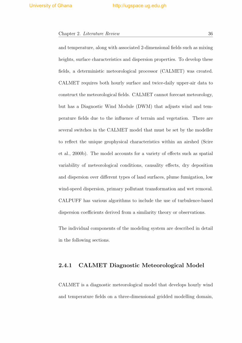
and temperature, along with associated 2-dimensional fields such as mixing
heights, surface characteristics and dispersion properties. To develop these
fields, a deterministic meteorological processor (CALMET) was created.
CALMET requires both hourly surface and twice-daily upper-air data to
construct the meteorological fields. CALMET cannot forecast meteorology,
but has a Diagnostic Wind Module (DWM) that adjusts wind and tem-
perature fields due to the influence of terrain and vegetation. There are
several switches in the CALMET model that must be set by the modeller
to reflect the unique geophysical characteristics within an airshed (Scire
et al., 2000b). The model accounts for a variety of effects such as spatial
variability of meteorological conditions, causality effects, dry deposition
and dispersion over different types of land surfaces, plume fumigation, low
wind-speed dispersion, primary pollutant transformation and wet removal.
CALPUFF has various algorithms to include the use of turbulence-based
dispersion coefficients derived from a similarity theory or observations.
The individual components of the modeling system are described in detail
in the following sections.
2.4.1 CALMET Diagnostic Meteorological Model
CALMET is a diagnostic meteorological model that develops hourly wind
and temperature fields on a three-dimensional gridded modelling domain,
University of Ghana http://ugspace.ug.edu.gh

Chapter 2. Literature Review 37
including two-dimensional fields such as mixing height, surface characteris-
tics and dispersion properties. The CALMET model operates in a terrain-
following vertical coordinate system using Eqn.(2.7):
Z = z − ht (2.7)
Where
Z is the terrain-following vertical coordinate (m),
z is the Cartesian vertical coordinate (m) and
ht is the terrain height (m).
The vertical velocity, W, in the terrain-following coordinate system is de-
fined by Eqn.(2.8):
W = w − u∂ht∂x− v∂ht
∂y(2.8)
Where
w is the physical vertical wind component (m/s) in Cartesian coordinates
and
u , v are the horizontal wind components (m/s).
The diagnostic wind field module in CALMET uses a two-step approach
in the computation of wind fields (Scire et al., 2000a). In the first step,
an initial-guess wind field is adjusted for kinematic effects of terrain, slope
University of Ghana http://ugspace.ug.edu.gh

Chapter 2. Literature Review 38
flows and terrain blocking effects to produce a Step-1 wind field. CALMET
parameterizes the kinematic effects of terrain using the approach of Liu and
Yocke (1980).
The Cartesian vertical velocity is computed by Eqn.(2.9):
w = (V · ∇ht)exp(−kz) (2.9)
Where
V is the domain-mean wind speed,
ht is the terrain height,
k is a stability-dependent, coefficient of exponential decay and
z is the vertical coordinate
The exponential decay coefficient, k, increases with increasing atmospheric
stability and is given by Eqn.(2.10):
k =N
|V |(2.10)
Where
|V | is the speed of the domain-mean wind and
N is the Brunt-Vaisala frequency (1/s) and is given by Eqn.(2.11):
University of Ghana http://ugspace.ug.edu.gh

Chapter 2. Literature Review 39
N =
[(g
θ)dθ
dz
] 12
(2.11)
Where
θ is the potential temperature (K) and
g is the acceleration due to gravity (m/s2)
The kinematic effects of the terrain on the horizontal wind components are
evaluated by applying a divergence-minimization procedure to the initial
guess of the wind field.
The thermodynamic blocking effects of terrain on the wind flow are param-
eterized in terms of the local Froude number given by Eqn.(2.12):
Fr =V
N∆ht(2.12)
Where
Fr is the local Froude number,
V is the wind speed(m/s) at the grid point,
N is the Brunt-Vaisala frequency (1/s) and
∆ht is the effective obstacle height(m) and is given by Eqn.(2.13):
∆ht = (hmax)ij − (z)ijk (2.13)
University of Ghana http://ugspace.ug.edu.gh

Chapter 2. Literature Review 40
Where
(hmax)ij is the highest gridded terrain height within a radius of influence of
the grid point (i,j) and
(z)ijk is the height of level k of grid point (i,j) above the ground.
The second step consists of an objective analysis procedure to introduce
observational data (surface and upper-level observational) into the step 1
wind field in order to produce the final wind field.
An option is provided to allow gridded prognostic wind fields to be used
by CALMET, which better represents regional flows and certain aspects
of sea breeze circulations. The prognostic data, as a 3D.DAT file, can be
introduced into CALMET in three ways: as a replacement for the initial
guess wind field, as a replacement for the step 1 field or as observations
in the objective analysis procedure. In order to improve the initialization
of the diagnostic model, the wind fields from the WRF prognostic model
are ingested every hour by CALMET as the initial-guess wind field. This
step is expected to improve the models performance by providing equally
spaced data points both at the surface and upper levels within the modelling
domain where observational data are not available (Chandrasekar et al.,
2003). The prognostic winds are interpolated to the fine-scale CALMET
grid. The diagnostic module in CALMET then adjusts the initial-guess
University of Ghana http://ugspace.ug.edu.gh

Chapter 2. Literature Review 41
wind field for kinematic effects of terrain, slope flows and terrain blocking
effects using fine-scale CALMET terrain data.
CALMET reads hourly surface observations of wind speed, temperature,
cloud cover, ceiling height, surface pressure, relative humidity, and precip-
itation (only if wet removal is to be computed). The twice-daily upper air
observations required by CALMET include vertical profiles of wind speed,
wind direction, temperature, pressure, and elevation. CALMET also re-
quires geophysical data, including gridded fields of terrain elevations and
land use categories. Gridded fields of other geophysical parameters, such as
the surface roughness length, albedo, Bowen ratio, soil heat flux parameter,
anthropogenic heat flux and vegetation leaf area index are also required.
CALMET consists of two boundary layer meteorological modules for over-
land and over water applications (Scire et al., 2000b). For overland sur-
faces, the energy balance method of Holtslag and Van Ulden (1983) is used
to compute hourly gridded fields of the heat flux, surface friction veloc-
ity, Monin-Obukhov length, and convective velocity scale. Mixing heights
are determined from the computed hourly surface heat fluxes and observed
temperature soundings. The model also determines the Pasquill-Gifford
stability classes and optional hourly precipitation rates.
University of Ghana http://ugspace.ug.edu.gh

Chapter 2. Literature Review 42
2.4.2 CALPUFF Model
The basic equation for the contribution of a puff at a receptor by CALPUFF
is by Eqn.(2.14):
C =Q
2πσxσyg
{exp
(−da2
2σ2x
)exp
(−d2c2σ2
y
)}(2.14)
Where
C is the ground-level concentration (g/m3),
Q is the pollutant mass (g),
σx, σy and σz are the standard deviations (m) of the Gaussian distribution
in the along-wind direction, cross-wind and vertical directions respectively,
da and dc are the distances (m) from the puff center to the receptor in the
along-wind and cross-wind directions respectively and
g is the vertical term (m) of the Gaussian equation.
The vertical term, g, is given by Eqn.(2.15):
g =2
(2π)12σz
∞∑n=−∞
exp[−(He + 2nh)2/(2σz
2)]
(2.15)
Where
He is the effective height (m) above the ground of the puff center and
University of Ghana http://ugspace.ug.edu.gh

Chapter 2. Literature Review 43
h is the mixed-layer height (m).
2.4.2.1 Dispersion
The key modelling consideration in CALPUFF is the specification of the
horizontal and vertical Gaussian dispersion coefficient, σy and σz, for a
puff (or each end of a slug) at the start and end of a sampling step, and
also for each receptor at which the cloud has a computed contribution
during the step. The coefficients for the puff location at the start of a
step are equal to those found at the end of the preceding sampling step,
because cloud-size is continuous between sampling steps. Those at the
end of the step, or at nearby receptors during the step, are computed
according to an ambient turbulence growth relationship and possibly a
source-related constant variance. The growth due to ambient turbulence
may be formulated as either a function of time, or as a function of distance.
Therefore, a generic metric ξ which stands for either one is used (Scire et al.,
2000b).
The dispersion coefficients for an incremental ’position’ ∆ξ, relative to the
beginning of sampling step n are given by Eqn.(2.16):
σ2y,n(∆ξy) = σ2
yt(ξyn + ∆ξy) + σ2ys + σ2
yb (2.16)
University of Ghana http://ugspace.ug.edu.gh

Chapter 2. Literature Review 44
and Eqn.(2.17):
σ2z,n(∆ξz) = σ2
zt(ξzn + ∆ξz) + σ2zb (2.17)
Where
ξyn and ξzn are the virtual-source metrics (time;distance) defined implicitly
by the requirement that the sigmas match those at the end of the previous
step when ∆ξ = 0,
σy,n and σz,n are the total horizontal and vertical dispersion coefficients (m)
respectively at some position during sampling step n,
σyt and σzt are the functional forms of the dispersion coefficients (m) of
σy and σz respectively due to atmospheric turbulence. σyb and σzb are the
components (m) of σy and σz respectively due to plume buoyancy at the
time of release and
σys is the component of the horizontal dispersion coefficient (m) due to the
lateral (cross-wind) scale of an area-source.
The increment ∆ξ is positive when describing the growth of the puff during
the sampling step, but can be either positive or negative for receptor-specific
sigmas. For example, ∆ξ would be negative for a receptor located just
upwind of the puff at the start of a sampling step. This allows CALPUFF
to reproduce plume-like features during steady meteorological conditions,
University of Ghana http://ugspace.ug.edu.gh

Chapter 2. Literature Review 45
using very few puffs. Negative ∆ξ could also drive the argument of σyt and
σzt through zero if a lower limit on the size of the sigmas at the source
were not enforced. So there is an initial ξ0 imposed, defined implicitly by
Eqn.(2.18) and Eqn.(2.19):
σ2yt(ξoy) = σ2
yo (2.18)
and
σ2zt(ξoz) = σ2
zo (2.19)
Where
σyo and (ξoz) are the initial values (m) of σy and σz respectively due to
the nature of the source (e.g., volume source) or the rapid initial dilution
associated with building downwash of point sources and
ξo is the initial virtual-source metric defined implicitly and separately for
y and z.
Thus, quadratic addition of initial dispersion components for buoyant rise
effects and for the lateral size of an area source are assumed, but other
initial cloud dimensions and the subsequent growth of the puff or slug are
accomplished using the virtual-distance or virtual-transport time approach.
This virtual- source approach is necessary if current puff growth is to be
dependent only on the current size of the puff and not on how it reached
University of Ghana http://ugspace.ug.edu.gh

Chapter 2. Literature Review 46
that size. The concept of a virtual source is particularly important when
a puff can move between substantially different dispersion regimes in just
one sampling step. For example, land use varies by grid cell, so a puff may
go from an overwater cell with weak dispersion into an overland cell with
substantial vertical convection. Or a young puff in the late afternoon mixed
layer may see the turbulence decay rapidly. In both cases, CALPUFF com-
putes subsequent growth during the step using the appropriate turbulence
(actual or parameterized), and the growth rate appropriate to its size (Scire
et al., 2000b).
2.4.2.2 Atmospheric Turbulence Components
In the calculation of the atmospheric turbulence components, the basic
strategy in the design of the dispersion module is to allow the use of the
most refined data available in the calculation of σyt and σzt. For situa-
tions in where this data is not available, backup algorithms not requiring
specialized data are provided. The five dispersion options are:
1. Dispersion coefficients computed from measured values of turbulence,
σv and σw.
2. Dispersion coefficients from internally calculated σv and σw using mi-
crometeorological variables.
University of Ghana http://ugspace.ug.edu.gh

Chapter 2. Literature Review 47
3. Pasquill-Gifford(PG) dispersion coefficients for rural areas (computed
using the Industrial Source Complex Short-Term (ISCST) multi-segment
approximation) and McElroy-Pooler coefficients in urban areas.
4. Same as 3 except PG coefficients are computed using the MESOPUFF
II equations.
5. Complex Terrain Dispersion Model(CTDM) sigmas used for stable
and neutral conditions (assumes that measured σv and σw are read).
For unstable conditions, sigmas are computed as in Dispersion Option
3.
2.4.2.3 Buoyancy-Induced Dispersion
The effect of plume buoyancy on the dispersion coefficients are parameter-
ized in terms of the plume rise (Irwin, 1983). It is given by Eqn.(2.20):
σyb = σzb =∆H
3.5(2.20)
Where
∆H is the plume rise(m).
Buoyancy-induced dispersion (BID) is automatically included for all the
dispersion coefficient options described in Section 2.4.2.2.
University of Ghana http://ugspace.ug.edu.gh

Chapter 2. Literature Review 48
The basic point source plume rise relationships are based on the Briggs
equations (Briggs, 1975). The plume rise due to buoyancy and momentum
during neutral or unstable conditions, zn is calculated using Eqn.(2.21):
zn =[3Fmx/(βj
2us2) + 3Fx
2/(2β12us
3)]1/3
(2.21)
Where
Fm is the momentum flux (m4/s2),
F is the buoyancy (m4/s3),
us is the stack height wind speed (m/s),
x is the downwind distance (m),
β1 is the neutral entrainment parameter (∼ 0.6),
βj is the jet entrainment coefficient (βj = 1/3 + us/w),
w is the stack gas exit speed (m/s).
During stable conditions, the plume rise, zs is determined by Eqn.(2.22):
zs =[3Fm/(βj
2usS1/2) + 6F/(β2
2usS)]1/3
(2.22)
Where
β2 is the stable entrainment parameter (∼ 0.36) and
University of Ghana http://ugspace.ug.edu.gh

Chapter 2. Literature Review 49
S is a stability parameter given by Eqn.(2.23):
S =
(g
Ta
)(dθ
dz
)(2.23)
Where
g is the acceleration due to gravity (m/s2),
Ta is the ambient temperature (K) and
(dθ/dz) is the potential temperature lapse rate (K/m).
2.4.3 CALPOST
CALPOST is used to process output files from CALMET and CALPUFF,
producing tabulations that summarize the results of the simulation, identi-
fying the highest and second highest 3-hour average concentrations at each
receptor for example. Fig. 2.5 is the schematic diagram of the CALPUFF
system.
The application of CALMET/CALPUFF modelling system is well known,
and several validation tests have been published (Dios et al., 2013, Dresser
and Huizer, 2011, Fishwick and Scorgie, 2011, Ghannam and El-Fadel, 2013,
Hernandez et al., 2014, Levy et al., 2003, Protonotariou et al., 2004). Most
of them were based on specific experiments with passive tracers and a
large compilation of surface and aloft meteorological measurements during
University of Ghana http://ugspace.ug.edu.gh

Chapter 2. Literature Review 50
Figure 2.5: A schematic diagram of the program elements in theCALMET/CALPUFF modelling (Scire et al., 2000b)
the experiments, in order to achieve the best model performance evalua-
tion. However, with actual pollutants sources and limited meteorological
datasets, uncertainties arise (both in measurements and models results)
and worse models performance is expected.
University of Ghana http://ugspace.ug.edu.gh

Chapter 2. Literature Review 51
2.4.4 Weather Research and Forecasting (WRF) Model
The WRF model is a fully compressible, non-hydrostatic mesoscale model
with a hydrostatic option which uses a terrain-following hybrid sigma-
pressure vertical coordinate in its meteorology simulation (Janjic, 2003,
Janjic, 2002). It was developed in a collaborative effort by the National
Center for Atmospheric Research (NCAR), the National Centers for En-
vironmental Prediction (NCEP), the Forecast Systems Laboratory (FSL),
the Air Force Weather Agency (AFWA), Oklahoma University (OU) and
other university scientists. It is a state-of-the-art numerical weather pre-
diction (NWP) and data assimilation system suitable for horizontal grid
scales in the 1 to 10 km range. The model can be run in a nested way with
the outer domain on a regional scale, covering distances usually between
500 1,000 km (Michalakes et al., 2004, Shamarock et al., 2008).
University of Ghana http://ugspace.ug.edu.gh

Chapter 3
Methodology
3.1 Introduction
This Chapter describes the study area for the research and the calculations
used in the estimation of the emissions from the Tema Oil Refinery. The
methodology employed in the meteorological and dispersion simulations are
also presented. The mass balance method is employed in the estimation
of pollutants from the RFCC unit of the refinery due to the unavailability
of such data from the refinery. Based on these calculated rates, emissions
from the whole refinery are also derived. The flare and flue stack are also
characterised by parameters such as stack/flare height and diameter, emis-
sion escape velocity and discharge temperature. The methodology used in
validating the CALPUFF/CALMET simulation results are also presented.
52
University of Ghana http://ugspace.ug.edu.gh

Chapter 3. Methodology 53
3.1.1 The Study Area
The study area, capturing Ghana’s only refinery in Tema, the emission
source for this study and spaning a domain size of 60 km × 60 km, is lo-
cated in the Greater Accra Region of Ghana stretching along the Ghanaian
Atlantic coast and extending a bit north into Ghana's interior as shown
by Fig.3.1. The Universal Transverse Mercator (UTM) coordinate of the
southwestern corner of the domain in zone 30 are 795 km easting and
600 km northing. The study area covers most part of the Accra Metropoli-
tan area, the Tema municipal area and extends to parts of the Eastern and
Volta regions. The southern boundary of the metropolis of Accra which
coincides with that of the study area is the Gulf of Guinea.
Tema is the most industrialised city in Ghana on the Gulf of Guinea and
Atlantic coast of Ghana. It is located 25 km east of the capital city, Accra,
in the region of Greater Accra with a population of approximately 402,637
people (G.S.S, 2012). Tema is locally nicknamed the ’Harbour Town’ be-
cause of its status as Ghana’s largest seaport. It is a major trading center,
home to Ghana’s only oil refinery and other numerous factories, and is
linked to Accra by a highway and railway.
The Greater Accra Region is located in the Dahomeyan Gap, where the
coast runs parallel to the prevailing moist monsoonal winds. It features
a tropical savanna climate and a savanna vegetation that borders on a
University of Ghana http://ugspace.ug.edu.gh

Chapter 3. Methodology 54
Figure 3.1: Map of Study Area showing the Tema Oil Refinery
University of Ghana http://ugspace.ug.edu.gh

Chapter 3. Methodology 55
semi-arid climate. Accra experiences two rainy seasons: April to June and
September to October with the former being the heaviest. The average
annual rainfall is about 730 mm which falls primarily during Ghana's two
rainy seasons. Variation in temperature throughout the year is recorded
to be nominal with mean monthly temperature ranging from 24.7◦C in
August to 28◦C in March and an annual average of 26.8◦C. Relative hu-
midity is generally high, varying from 65% in the mid afternoons to 95%
at night. Accra experiences a breezy dry heat during windy harmattan
seasons usually in December and January (Muff and Efa, 2006).
The landscape is mainly flat with terrain elevations between 200 m and
500 m, except for the low mountain system (Akropong range north of the
refinery and the Shai hills) east of the refinery. The traditional land use clas-
sification within the study area includes built-up/urbanisation, forestry/a-
griculture, water, shoreline, protected areas and bare areas inferred from
Addo (2013).
3.1.2 Tema Oil Refinery
Tema Oil Refinery (TOR) Limited, formerly Ghanaian Italian Petroleum
(GHAIP) Limited was commissioned on December 12, 1963. The Gov-
ernment of Ghana became the sole shareholder in 1977 and renamed the
company Tema Oil Refinery Limited in 1991. The Refinery predominantly
University of Ghana http://ugspace.ug.edu.gh

Chapter 3. Methodology 56
processes crude oil into refined products like LPG, Gasoline, Jet Fuel,
Kerosene, Diesel and Fuel Oils. The refinery is situated on an area of
440,000 square meters located in the industrial hub of the Greater Accra Re-
gion. The refinery complex, as a whole, contains the refinery itself, its tank
farm containing storage tanks, wastewater treatment plant, gas turbine
power generating sets and its utility system of boilers. The refinery has an
installed total capacity of 65 000 barrels per stream day(bpsd) equivalent to
3,000,000 tonnes per annum (tpa) with contributions from the Crude Distil-
lation Unit (CDU)- 2,000,000 tpa, Residue Fluid Catalytic Cracker(RFCC)-
685,000 tpa and the Premium Reforming unit(PRF)-315,000 tpa (Darko
and Quist, 2012).
The RFCC process converts heavy crude oil fractions into lighter, more
valuable hydrocarbon products at high temperature and moderate pressure
in the presence of finely divided silica/alumina based catalyst in crude
refineries. In the course of cracking the large hydrocarbon molecules into
smaller molecules, a non-volatile carbonaceous material, commonly referred
to as coke, is deposited on the catalyst. The presence of coke on the catalyst
deactivates the catalytic cracking activity of the catalyst by blocking access
to the active catalytic sites. In order to regenerate the catalytic activity
of the catalyst, the coke deposited on the catalyst is burned off with air in
the regenerator vessel. The regenerator is normally operated at conditions
that achieve complete combustion of C to CO2. Flue gas exits the cyclone
University of Ghana http://ugspace.ug.edu.gh

Chapter 3. Methodology 57
separators to minimize catalyst entrainment prior to discharge from the
regenerator through the flue stack (Maya-Yescas et al., 2005). Other stack
emissions include SOx, NOx and unburnt hydrocarbons.
The refinery is also equipped with a flare which primarily burns off flammable
gas released by pressure relief valves during unplanned over-pressuring of
plant equipment. It is used both for safety reasons during process upsets
(start-up, shut down, system blow-down) and for managing the disposal of
waste gases with hydrocarbons from routine operations. However, through
combustion, the flare also produces other pollutants including SOx, NOx,
CO, CO2 and PM (both total PM and micro-particulates- ie, PM10 and
PM2.5). Infact, according to USEPA (2011), it is one of the air pollution
sources in a refinery emission inventory followed by the flue stack. It is
for this reason that other emissions from stationary combustion sources,
including process heaters, boilers, combustion turbines and similar devices,
are not calculated but extrapolated, in this study.
3.2 Tema Oil Refinery Emission Estimation
The air emissions from the refinery are mainly due to the combustion of
fuel gas. In this work, the pollutants of interest are SOx, NOx, CO2, PM
and VOCs and the point sources under consideration are the flue stack and
the flare. As mentioned early on, the mass balance approach is employed
University of Ghana http://ugspace.ug.edu.gh

Chapter 3. Methodology 58
Table 3.1: Operational Average Flow Parameters of the RFCCU ofthe Tema Oil Refinery for 2008 - 2013
Year Feed Rate Airflow Rate Fuel Gas rate Initial Catalyst(m3/hr) (Nm3/hr) (kg/hr) Inventory(kg/hr)
2008 78.83 70989.00 6248.93 1200002009 72.02 63882.88 6239.00 1200002010 80.11 63147.37 6858.40 1200002011 73.44 56954.83 6368.20 1200002012 74.71 55508.67 5853.17 1200002013 74.44 55643.80 5207.14 120000
during which the compound being combusted is examined to predict the
emissions. The gases involved in the calculations were assumed to be ideal
and so the idea gas laws were applied.
For example, the flue stack gas contains products of the combustion of
deposited carbon on the catalyst during cracking. Based on the stoichio-
metric equations of the combustion reactions, products are estimated given
the reactant concentrations. In the case of the flare, emissions rates are in-
formed by a gas chromatographic analysis of the fuel gas exiting the flare.
Table 3.1 shows the quantities of some parameters used in the calculations.
3.2.1 Estimation of Flue Stack Gas Rate and Com-
position
In the regeneration of the catalyst in the regenerator through combustion,
air is used as a source of oxygen. The carbon reacts to form CO2 upon com-
plete combustion as is the case with this refinery. Based on the regenerator
University of Ghana http://ugspace.ug.edu.gh

Chapter 3. Methodology 59
air flow rate, therefore, the emission rates of CO2 and carbon particulates
are estimated. The air flow rate provided by the refinery is on a wet basis
and was converted to dry basis prior to the calculations.
The larger component of the total FCC PM emitted is as a result of cyclone
inefficiency estimated at 0.25% (Harding et al., 2001, Jimenez-Garcıa et al.,
2011) which is what is used in the calculations. Research also shows that
PM2.5 is a large fraction of the total particulate emissions even without
consideration of primary sulphate or organic emissions (England et al.,
2000, Hildemann et al., 1994). Therefore, PM modelled in this study is
considered to be of aerodynamic diameter of 2.5.
According to Corma et al. (1997), in the FCC unit, between 45 and 55%
of the total sulphur present in the feed, especially the nontiophenic com-
pounds, is converted to H2S, while approximately 35 to 45% stays in the
liquid products as sulphur compounds. The remaining 5% is left on the
catalyst as part of coke and results in 90% SO2 and 10% SO3 during the
coke combustion. The TOR processes mainly light sweet and light sour
crude with % feed sulphur between 0.5 - 1.5 (Darko and Quist, 2012, Prod-
ucts, 1997, Zhao et al., 1997). In this study, an average of 1% feed sulphur
is used.
Elemental nitrogen typically equals 0.32% of the FCC feed, 15% of which
ends up on the catalyst together with the coke. Ninety percent (90%) of
University of Ghana http://ugspace.ug.edu.gh

Chapter 3. Methodology 60
this is converted to NO and the remaining 10% to NO2 and ends up in the
flue gas (Jimenez-Garcıa et al., 2011, Zhao et al., 1997).
A sample of the calculations, using flow parameters for the year 2009, are
shown in Appendix A.
3.2.2 Estimation of Flared Gas Composition
When fuel is burnt, carbon in the fuel reacts to form either CO2 or CO,
hydrogen forms H2O, sulphur forms SO2 and SO3 and some of the nitrogen
in the air forms NO2 at high temperatures (Abdul-Wahab, 2003, Corma
et al., 1997). However, when flaring is done in the presence of excess air,
CO is not formed which is the case in this study. Small amounts of NO2
are formed at temperatures greater than 1400◦C. Since this temperature
is greater than the flare temperature, it is also assumed that no NO2 is
produced in the flare. The flare emissions therefore contain H2, O2, N2,
CO2, SO2 and some unburnt hydrocarbons hereafter referred to as volatile
organic compounds (VOCs). VOCs are present in flare emissions as a re-
sult of flare efficiency (destruction efficiency) given as 98% (TOR Manual).
Flares are designed to operate at 98 - 99% (Al-Fadhli et al., 2011, Martın
et al., 2003, Wood et al., 2012). In this methodology, the composition of
the flare gas combustion products is calculated through atomic and molec-
ular balances. At constant temperature and pressure, mole % of gases is
University of Ghana http://ugspace.ug.edu.gh

Chapter 3. Methodology 61
equal to volume %. Therefore from the GC analysis report provided by
the quality control laboratory of the refinery, the mole fractions of the flare
gas components are calculated as shown in Appendix A. Given the average
molecular weight of the fuel gas of 20 kg/kmol (Zadakbar et al. (2008))
and its mass flow rate, the total moles of the fuel gas mixture are also
calculated. From this, the moles of the components are estimated using
their respective fractions. Based on the stoichiometry of the combustion
reactions, the combustion products are obtained: CO2, H2O, SO2 and N2.
SO2 and VOCs are the flare pollutants considered. Again, the estimation is
carried out using operational data for 2009 on an hourly basis and is shown
in Appendix A.
Total refinery emissions are then estimated as percentages of the RFCC
emissions (EIPPCB, 2012). For the sake of simplicity, SO2 and SO3 from
the flue stack are added and considered as SO2. Similarly, NO and NO2
are also lumped together and modelled as NO2.
3.2.3 Calculation of Flare and Flue stack Exit Gas
Velocities
The flare and flue gas velocities are calculated by dividing their volumetric
flow rates by the cross-sectional areas (obtained from their diameters) of
University of Ghana http://ugspace.ug.edu.gh

Chapter 3. Methodology 62
the flare stack and flue stack respectively. The calculations are shown in
Appendix A.
3.2.4 Modelling Period
A minimum of a year is necessary to capture the time-varying emissions
and meteorology during a full cycle of seasons. However, to be able to do a
trend analysis to inform future predictions, a six-year period from January
2008 to December 2013, was considered in the study.
3.2.5 Model Set-up
As stated earlier in this section, the key program elements and data in-
put requirements for CALPUFF are meteorological wind fields, emissions
data, receptor locations (points in the modeling domain where the model
will predict concentrations), and CALPUFF modeling parameters. These
elements are described below.
3.2.5.1 CALMET Modelling
Due to the unavailability of complete observational meteorological datasets
from the local weather stations, the CALMET model was initialised with
WRF data to develop the meteorological field for CALPUFF. This option is
University of Ghana http://ugspace.ug.edu.gh

Chapter 3. Methodology 63
available in the CALMET model. Because the prognostic models like WRF
are usually run over very large domains with much coarser resolutions, they
are not suitable for direct use in CALPUFF. In this case, CALMET will
interpolate the gridded prognostic data to develop a 3-D fine scale field of
wind speeds, directions and other parameters.
The WRF model runs were performed at the International Centre for The-
oretical Physics (ICTP), Trieste, Italy. Two one-way nested computational
domains were set with horizontal grid spacing of 24 and 12 km represent-
ing horizontal grid dimensions of outer and inner domains respectively as
shown in Fig.3.2. The vertical grid contained 29 full sigma levels. The
inner domain covered the whole of Ghana within which the study area is
located.
The model was run with Global Forecast System (GFS) 1 degree reanalysis
as initial and boundary conditions with full physics processes included in
order to reproduce real meteorological phenomena. Other options include
WRF Single Momentum (WSM) 6 Class Graupel for Microphysics Scheme,
Rapid Radiative Transfer Model (RRTM) scheme for long wave radiation,
Dudhia scheme for short wave radiation, Monin-Obukhov scheme for sur-
face layer, and Noah model (5 soil layers) for land-surface interactions,
while the dynamic options were left as default to produce hourly averages
(Skamarock et al., 2005).
University of Ghana http://ugspace.ug.edu.gh

Chapter 3. Methodology 64
Figure 3.2: Nested Computational domains in the WRF simulations
CALMET-compatible 3D.DAT files containing data of horizontal and ver-
tical velocity components, pressure, temperature and precipitation among
others were then created by running CALWRF on the WRF output data.
The CALMET meteorological processor was then used to interpolate the
12 km resolution WRF winds to the CALPUFF domain.
University of Ghana http://ugspace.ug.edu.gh

Chapter 3. Methodology 65
A horizontal grid spacing of 1 km was selected for the CALMET simula-
tion; the study area therefore corresponds to 60 rows by 60 columns. With
this grid spacing, it was possible to maximize run time and file size efficien-
cies while still capturing large-scale terrain feature influences on wind flow
patterns. CALMET uses fewer vertical layers than WRF, in part because
air pollution modeling does not require detailed information on the upper
atmosphere. Therefore to adequately characterize the vertical structure of
the atmospheric boundary layer (i.e., the layer within about 2000 metres
above the Earth's surface), ten vertical layers with cell face heights at 0,
20, 40, 80, 160, 320, 640, 1000, 1500, 2200 and 3000 m were used in the
CALMET runs. CALMET defines a vertical layer as the midpoint between
two faces (i.e., 11 faces correspond to 10 layers, with the lowest layer always
being ground level or 10 m). CALMET automatically interpolated from
the WRF model grid system to the CALMET grid (Scire et al., 2000a,
Zhou et al., 2003).
3.2.5.2 Geophysical Data Input
Prior to running CALMET, a geophysical file containing information about
the land use type, elevation and surface parameters about the domain un-
der study was created. Due to the unavailability of terrain elevation and
land use land cover (LULC) data in the required format for Ghana from the
local agency in the required format, data from the United States Geological
University of Ghana http://ugspace.ug.edu.gh

Chapter 3. Methodology 66
Survey (USGS) web site at
http://edcwww.cr.usgs.gov/doc/edchome/ndcdb/ndcdb.html was used.
Detailed terrain features were incorporated using the USGS global 3 arc-sec
SRTM3 data (∼ 90m resolution). Elevations are in meters relative to mean
sea level. The spacing of the elevations along each profile is 3 arc-seconds,
which corresponds to a spacing of approximately 90 meters. A vertical and
horizontal grid spacing of 1km was selected to adequately represent the
important terrain features. The raw terrain data were processed into each
gridded field. These terrain fields effectively resolve major land features in
the model domain.
Land use and land cover (LULC) data were downloaded from the USGS
at the 1:250,000-scale with file names corresponding to the 1:250,000-scale
map names. Land use data were processed to produce a 1-km resolution
gridded field of fractional land use categories and land use weighted values
of surface and vegetation properties for each CALMET grid cell. The 14
default CALPUFF land use categories were used (10, 20, 30, 40, 51, 54, 55,
60, 61, 62, 70, 80, and 90). Each land use type has six assigned values, one
each for surface roughness, albedo, Bowen ratio, soil heat flux parameter,
anthropogenic heat flux, and leaf area index. The surface roughness is a
measurement of the average vertical relief and small-scale irregularities of
the terrain surface. The surface roughness is low for the areas in the study
area classified as water bodies and is high for the areas classified as urban or
University of Ghana http://ugspace.ug.edu.gh

Chapter 3. Methodology 67
built-up land and forest. The albedo is the fraction of light that is reflected
by a given surface. For instance, the albedo of a snow-covered area is much
higher than that of a paved parking lot. The leaf area index is the ratio of
the total area of all leaves on a plant to the area of ground covered by the
plant. All areas that have the potential to have plant growth have leaf area
indexes assigned to them. A value of zero is assigned to the water bodies.
The leaf area index is as high as seven (7) in the areas identified as forest
land.
Terrain and land Use data for the modelling domain were then processed
through the TERREL and CTGPRO CALMET pre-processors respectively.
Since the modeling domain spans both over-water and over-land regions,
the global self-consistent hierarchical high-resolution shoreline (GSHHS)
was used to define the coastal lines. The CALMET GEO file was then cre-
ated using the MAKEGEO pre-processor which combines data from TER-
REL and CTGPROG.
CALMET was configured with the default wind field options and parame-
ters.
University of Ghana http://ugspace.ug.edu.gh
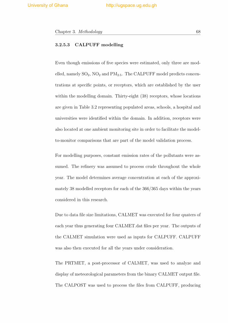
Chapter 3. Methodology 68
3.2.5.3 CALPUFF modelling
Even though emissions of five species were estimated, only three are mod-
elled, namely SO2, NO2 and PM2.5. The CALPUFF model predicts concen-
trations at specific points, or receptors, which are established by the user
within the modelling domain. Thirty-eight (38) receptors, whose locations
are given in Table 3.2 representing populated areas, schools, a hospital and
universities were identified within the domain. In addition, receptors were
also located at one ambient monitoring site in order to facilitate the model-
to-monitor comparisons that are part of the model validation process.
For modelling purposes, constant emission rates of the pollutants were as-
sumed. The refinery was assumed to process crude throughout the whole
year. The model determines average concentration at each of the approxi-
mately 38 modelled receptors for each of the 366/365 days within the years
considered in this research.
Due to data file size limitations, CALMET was executed for four quaters of
each year thus generating four CALMET.dat files per year. The outputs of
the CALMET simulation were used as inputs for CALPUFF. CALPUFF
was also then executed for all the years under consideration.
The PRTMET, a post-processor of CALMET, was used to analyze and
display of meteorological parameters from the binary CALMET output file.
The CALPOST was used to process the files from CALPUFF, producing
University of Ghana http://ugspace.ug.edu.gh
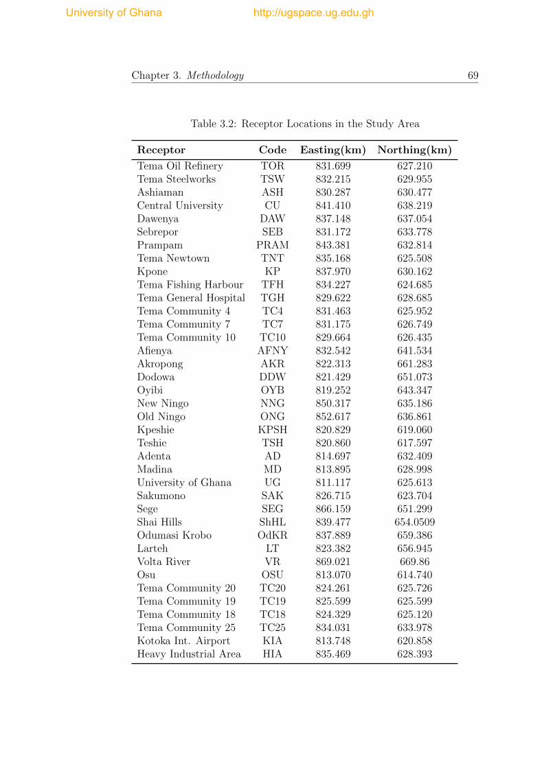
Chapter 3. Methodology 69
Table 3.2: Receptor Locations in the Study Area
Receptor Code Easting(km) Northing(km)
Tema Oil Refinery TOR 831.699 627.210Tema Steelworks TSW 832.215 629.955Ashiaman ASH 830.287 630.477Central University CU 841.410 638.219Dawenya DAW 837.148 637.054Sebrepor SEB 831.172 633.778Prampam PRAM 843.381 632.814Tema Newtown TNT 835.168 625.508Kpone KP 837.970 630.162Tema Fishing Harbour TFH 834.227 624.685Tema General Hospital TGH 829.622 628.685Tema Community 4 TC4 831.463 625.952Tema Community 7 TC7 831.175 626.749Tema Community 10 TC10 829.664 626.435Afienya AFNY 832.542 641.534Akropong AKR 822.313 661.283Dodowa DDW 821.429 651.073Oyibi OYB 819.252 643.347New Ningo NNG 850.317 635.186Old Ningo ONG 852.617 636.861Kpeshie KPSH 820.829 619.060Teshie TSH 820.860 617.597Adenta AD 814.697 632.409Madina MD 813.895 628.998University of Ghana UG 811.117 625.613Sakumono SAK 826.715 623.704Sege SEG 866.159 651.299Shai Hills ShHL 839.477 654.0509Odumasi Krobo OdKR 837.889 659.386Larteh LT 823.382 656.945Volta River VR 869.021 669.86Osu OSU 813.070 614.740Tema Community 20 TC20 824.261 625.726Tema Community 19 TC19 825.599 625.599Tema Community 18 TC18 824.329 625.120Tema Community 25 TC25 834.031 633.978Kotoka Int. Airport KIA 813.748 620.858Heavy Industrial Area HIA 835.469 628.393
University of Ghana http://ugspace.ug.edu.gh

Chapter 3. Methodology 70
a summary of simulation results in tabulated as well as in gridded form
CALPOST was also used to produce wind roses from the CALMET and
WRF output data.
3.2.5.4 Model Evaluation
The most commonly used measures of model performance are the statistics
recommended in the U.S.EPA 1992 modeling guidance. To determine the
reliability of the simulation data, verification of simulated values using the
WRF and CALMET models was conducted for surface wind speed and
direction. Datasets from the Tema and Accra meteorological stations were
used. Even though there are other stations located within the study do-
main, many of them are not functional. Therefore, only the two stations
mentioned were used. Due to the large number of missing data of the other
surface wind parameters, they could not be used for validation. Only wind
speed and direction were validated.
To validate the dispersion model, CALPUFF, measured data on SO2, NO2
emissions made from the 10 - 23 January, 2008 were used. The Differen-
tial Optical Absorption System (DOAS) used for the measurements was
installed on the premises of the Tema Oil refinery to monitor and measure
University of Ghana http://ugspace.ug.edu.gh

Chapter 3. Methodology 71
the concentration of gases emitted into the atmosphere due to its activi-
ties and also due to the operations of other industries within its environs.
Details of the set-up and results can be obtained in Sackey (2012).
The statistical verification of model performance in this study was per-
formed using four statistical indicators including the Index of Agreement
(IOA), Fractional Bias (FB), Normalized Mean Square Error (NMSE), and
Pearson correlation coefficient (R). The formulas used to derive these five
indicators are given in :Eqn. 3.1 - Eqn. 3.3.
R =
N∑i=1
(Coi − Co
)(Cpi − Cp
)√σoσp
(3.1)
FB =Co − Cp
0.5(Co + Cp
) (3.2)
NMSE =
(Co − Cp
)2CoCp
(3.3)
IOA = 1−
N∑i=1
(Cpi − Coi
)2N∑i=1
( ∣∣Cpi − Co
∣∣+∣∣Coi − Cp
∣∣ )2 (3.4)
University of Ghana http://ugspace.ug.edu.gh

Chapter 3. Methodology 72
where Co is the observed quantity, Cp the predicted quantity, Coi and Cpi
are the observed and predicted quantities respectively for N cases.
University of Ghana http://ugspace.ug.edu.gh

Chapter 4
Results and Discussions
4.1 Introduction
This Chapter presents results of the estimated refinery emission rates and
other parameters used for the dispersion simulations. Both the meteoro-
logical and dispersion simulation results are also presented and discussed
as well as their validation.
4.2 Refinery Emissions and Interannual Trends
Plots of estimated emission rates of CO2, VOCs, PM2.5, SO2 and NO2 and
their averages for 2008 - 2013 are shown in Figs.4.1 - Fig.4.5 respectively.
It can be noticed that total CO2 emissions were the highest of the pollutants
estimated from the Tema Oil Refinery ranging from about 130 to 165 t/hr.
73
University of Ghana http://ugspace.ug.edu.gh

Chapter 4. Results and Discussions 74
Figure 4.1: Interannual Variation of CO2 Emission Rates from theTema Oil Refinery
Figure 4.2: Interannual Variation of VOCs Emission Rates fromthe Tema Oil Refinery
The VOCs are next in line with emission rates ranging between 2083 and
2500 kg/hr. Particulate matter rates were observed to decline marginally
over the years with an average rate of 1032 kg/hr followed by SO2 and NO2
with average rates of 776 and 371 kg/hr respectively.
CO2 emissions were highest in 2008, dipped in 2009, increased again in
2010 after which a steady decrease over the remaining years is observed.
The highest emissions of PM2.5 also occured in 2008 followed by a marginal
University of Ghana http://ugspace.ug.edu.gh

Chapter 4. Results and Discussions 75
Figure 4.3: Interannual Variation of PM2.5 Emission Rates fromthe Tema Oil Refinery
Figure 4.4: Interannual Variation of SO2 Emission Rates from theTema Oil Refinery
steady decline over the years. However, the other emissions peaked in 2010
and declined steadily over the following years. The decline in emission rates
was a result of a reduction in production due to the frequent shortfalls in
the refinery’s crude oil supply, consequently leading virtually to a halt of
refinery operations in 2014 preceded by intermittent shutdowns.
University of Ghana http://ugspace.ug.edu.gh

Chapter 4. Results and Discussions 76
Figure 4.5: Interannual Variation of NO2 Emission Rates from theTema Oil Refinery
4.3 Preliminary Dispersion Simulation
Geophysical inputs, terrain data (with receptor locations relative to the
refinery) and Land Use data, are given Figs.4.6 and 4.7 respectively.
The most prominent topographical feature is the Gulf of Guinea that forms
the southern boundary of the study area. The other topographical feature
with elevated terrain, between 300 - 600 m, is the Akropong-range located
at the north-western corner of the study area as shown in Fig.4.6. Land
use within the study area is fairly complex, varying from open ocean to
the south, marshy and wetlands along the coast to the urban areas of Osu
(Fig.4.7). The built-up Tema community is not captured probably due to
poor resolution. In addition, there are large tracts of agricultural land also
present in the study area.
University of Ghana http://ugspace.ug.edu.gh

Chapter 4. Results and Discussions 77
Figure 4.6: Terrain Map of the Study area showing receptor loca-tions and the Refinery (red square)
Figure 4.7: LandUse Map of the Study Area
University of Ghana http://ugspace.ug.edu.gh

Chapter 4. Results and Discussions 78
4.3.1 Spatial Variation of Pollutants
Results of the preliminary simulations of the dispersion of the refinery emis-
sions in the study domain are presented in the form of daily average con-
centrations of the modelled emissions at the indicated receptors respec-
tively. Considering the receptor locations within the study area, as shown
in Fig.4.6, it was observed that predicted daily average pollutant concen-
trations were high at receptors closest to the refinery and low at receptors
far away from the refinery. This can be explained by the dispersion equa-
tion, Eqn.(2.14), which expresses an exponential decay of emissions with
distance from emission source.
Considering receptor locations relative to the refinery, predicted concen-
trations were noted to be high at northern receptors as seen in Fig.4.8.
These receptors include Tema Steelworks, Ashiaman and Sebrepor. This
was followed by receptors on the north-eastern side up to about 10 km of
the refinery including Heavy Industrial Area, Dawenya, Kpone, Prampam,
Old and New Ningo and the Central University as shown in Fig.4.9. Tema
Newtown and the Tema Fishing Harbour located south east of the refin-
ery also receive significant emissions followed by south western receptors
including Tema Communities 4, 7 and 10 and the Tema General Hospi-
tal which are located within a distance of about 4 km of the refinery as
shown in Figs.4.10 and 4.11. Receptors located on the north western part
University of Ghana http://ugspace.ug.edu.gh

Chapter 4. Results and Discussions 79
Figure 4.8: Predicted Daily Average Concentrations of SO2, NO2
and PM2.5 at northern receptors in the Study area
Figure 4.9: Predicted Daily Average Concentrations of SO2, NO2
and PM2.5 at north eastern receptors in the Study area
of the refinery are the least impacted by the refinery emissions as they
showed very low emission concentrations. These include Madina, Adenta,
the University of Ghana, Oyibi, Larteh, Dodowa and Akropong.
University of Ghana http://ugspace.ug.edu.gh

Chapter 4. Results and Discussions 80
Figure 4.10: Predicted Daily Average Concentrations of SO2, NO2
and PM2.5 at south eastern receptors in the Study area
Figure 4.11: Predicted Daily Average Concentrations of SO2, NO2
and PM2.5 at south western receptors in the Study area
University of Ghana http://ugspace.ug.edu.gh

Chapter 4. Results and Discussions 81
Figure 4.12: Predicted Daily Average Concentrations of SO2, NO2
and PM2.5 at northern western receptors in the Study area
The prevailing wind directions during the year under study were south-
westerly (87%) of total winds as depicted by Fig.4.13. Therefore, receptors
located on the north and north-eastern parts of the refinery show relatively
higher emission concentrations than other parts of the study domain be-
cause the south-westerly winds carry the pollutant clouds from the refinery
towards them. Approximately 77% of winds in the study area are clustered
in 3rd wind speed classes (3.3 - 5.4 m/s) with winds in the next upper class
of (5.4 - 8.5 m/s) being 19%. Winds from 1.8 - 3.3 m/s account for 8% of
total winds. The average wind speed is estimated at 3.45 m/s with calm
winds forming 0.057% of total winds.
Based on these preliminary results, it can be concluded that emissions from
the refinery impact communities located within a radius of about 10-15 km
around the refinery. Consequently, subsequent simulations of emissions of
University of Ghana http://ugspace.ug.edu.gh

Chapter 4. Results and Discussions 82
Figure 4.13: Wind Rose Depicting Surface Winds in Tema for 2008
the other years will focus on the receptors which fall within this radius of
influence.
4.4 Validation of the CALPUFF Model
At this point, results of the performance evaluation of CALPUFF, are
presented and discussed. Plot of the comparison between measured and
modelled SO2 and NO2 are seen in Fig.4.14 and Fig.4.15 respectively.
The performance assessment of the model, based on direct quantitative
comparisons of observed and predicted mean concentrations as seen in
University of Ghana http://ugspace.ug.edu.gh
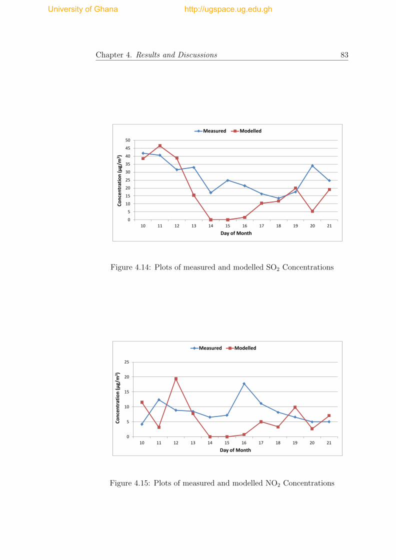
Chapter 4. Results and Discussions 83
0
5
10
15
20
25
30
35
40
45
50
10 11 12 13 14 15 16 17 18 19 20 21
Co
nce
ntr
atio
n (
µg/
m3)
Day of Month
Measured Modelled
Figure 4.14: Plots of measured and modelled SO2 Concentrations
0
5
10
15
20
25
10 11 12 13 14 15 16 17 18 19 20 21
Co
nce
ntr
atio
n (
µg/
m3)
Day of Month
Measured Modelled
Figure 4.15: Plots of measured and modelled NO2 Concentrations
University of Ghana http://ugspace.ug.edu.gh

Chapter 4. Results and Discussions 84
Figs.4.14 and 4.15, reveals that CALPUFF predictions for SO2 were bet-
ter than NO2 concentrations. From the 10 - 12, 17 - 19 and 21 January,
predicted SO2 concentrations closely approached measurements. Quanti-
tative agreement between predicted and modelled NO2 concentrations is
excellent on 13 January and good for 19 - 21. However, from 13-16 Jan-
uary, CALPUFF significantly under-predicted the measured values. De-
spite these differences between predicted and measured values on some
days, the trends in the measurements are accurately predicted especially
for SO2. The simulation results did not take into account SO2 and NO2
background concentrations because this data was not available. This may
explain the reason for this under-prediction. The measured concentrations
are likely to include emissions from other sources which are not considered
in the simulations. Another important reason could be the assumption
made that emission rates from the refinery are constant. This is unlikely
to be representative of actual operating conditions at the refinery. It was,
however, necessary to make this assumption using a constant estimated
average emission rates for modeling purposes. Additionally, possible errors
associated with the measurements of SO2 and NO2 at the measurement
location cannot be overlooked.
Results of model performance evaluation after applying the USEPA guide-
lines pertaining to model evaluation protocol are presented in Table 4.1.
The indices are the correlation coefficient (R), the index of agreement
University of Ghana http://ugspace.ug.edu.gh

Chapter 4. Results and Discussions 85
(IOA), the normalised mean square error (NMSE) and the fractional bias
(FB).
Table 4.1: Statistical Performance Indices of the CALPUFF model
Pollutant R NMSE IOA FB
SO2 0.66 0.73 0.39 0.41NO2 -0.25 0.36 1.34 0.36
The index of agreement between predicted concentrations and measure-
ments is better for SO2 and NO2. The correlation coefficient of SO2 with
observations is satisfactory but that for NO2 is negatively weak as shown
in Table 4.1. The NO2 emissions from automobiles make up a large frac-
tion of ambient NO2 levels. It is therefore probable that a large fraction of
the measurements consists of contributions from the vehicular emission, re-
vealed in the weak correlation and the poor index of agreement. CALPUFF
under-predicts NO2 by a smaller factor than SO2 as revealed by their FB
values. The NMSE values for SO2 is acceptable whiles that of NO2 is not.
Therefore, based on these indices, the performance of CALPUFF can be
described as good.
University of Ghana http://ugspace.ug.edu.gh

Chapter 4. Results and Discussions 86
4.5 Validation of CALMET and WRF
Models
Results obtained from CALMET and WRF simulations are compared with
available surface observations (wind speed and direction) for January 2008
from the Tema meteorological station (TMS) as shown in Figs.4.16 and
4.17. Wind roses generated from the models for the same period are also
presented in Figs.4.18 and 4.19.
Figure 4.16: Plots of Observed and Modelled Wind Speeds
It is apparent from Fig.4.16 that WRF and CALMET models generally
under-predicted wind speeds from January 9 - 14 and over-predicted speeds
on January 16 - 24. However, on days 11, 16, 21 and 23, CALMET predic-
tions closely approach observations whiles WRF predicts similar speed on
University of Ghana http://ugspace.ug.edu.gh

Chapter 4. Results and Discussions 87
Figure 4.17: Plots of Observed and Modelled Wind Direction
the 15th January. Fig. 4.17 reveals the over-prediction of wind direction by
both models for most part of the period considered. From the other sta-
tistical performance measures given in Table 4.2, it can be observed that
both CALMET and WRF share similar indices rating their performances
on the same scale with CALMET indicating slightly higher correlation co-
efficients for both wind direction and speed than WRF. Under-prediction
by CALMET is greater than by WRF as seen in the FB values.
Table 4.2: Statistical Performance Indices of CALMET and WRFmodels
CALMET WRFParameter R NMSE IOA FB R NMSE IOA FB
Speed 0.58 0.66 0.24 0.34 0.57 0.65 0.09 0.15Direction 0.29 0.66 0.02 -0.10 0.28 0.66 0.02 -0.10
University of Ghana http://ugspace.ug.edu.gh

Chapter 4. Results and Discussions 88
Figure 4.18: Wind Rose Depicting CALMET Surface Winds
The wind rose generated from CALMET (Fig.4.18) indicated the predom-
inant prevailing wind is south south-westerly (26%) whiles southerly and
southwesterly represent about 26%. The remaining winds are spread across
a wide spectrum ranging from westerly to north north-easterly. WRF wind
rose (Fig.4.19) predicted an increased percentage of south south-westerly
winds (31%) than CALMET. It also indicates 12% of southerly winds and
12% of south-westerly winds which is lower than CALMET. It is clear that
the percentages of the other winds are also lower in the WRF wind rose than
University of Ghana http://ugspace.ug.edu.gh

Chapter 4. Results and Discussions 89
Figure 4.19: Wind Rose Depicting WRF Surface Winds
the CALMET. The predominant wind speed class predicted by both models
is 3.3 - 5.4 m/s with CALMET predicting a higher percentage (75%) than
WRF (64%). Thirty percent (30%) of the total winds have speeds between
5.4 - 8.5 m/s according to WRF whiles CALMET predicts only 3% of that
class. Generally, average wind speeds is higher for WRF than CALMET.
Calm winds in both modelled wind (>0.5 m/s) account for only 0.28% of
the data. Based on the statistics, it appears that CALMET predictions
better approximates observations as it is able to capture small scale effects
University of Ghana http://ugspace.ug.edu.gh

Chapter 4. Results and Discussions 90
which cannot be accounted for by WRF. Numerical meteorological models
tend to have spatial and temporal phase errors in simulating surface wind.
This is because the lowest-level WRF winds must be extrapolated down
to ground-level to initialize CALMET. Thus unless the vertical resolution
is quite fine, it would be expected that the near-surface CALMET output
winds will be biased towards the trends seen in the lowest level of the WRF
data, which has a higher elevation in the region compared to the surface
stations (Protonotariou et al., 2004). On this basis, the remaining valida-
tion results for only CALMET with data from TMS and AMS for 2008 -
2013 are presented in Table 4.3.
Table 4.3: Statistical Performance Indices of CALMET and Obser-vations from the TMS and AMS
TMS AMSYear Parameter R NMSE IOA FB R NMSE IOA FB
2008 Speed 0.58 0.24 0.66 0.34 0.56 0.88 0.72 0.08Direction 0.29 0.02 0.66 -0.10 0.57 0.02 0.71 -0.14
2009 Speed 0.48 0.12 0.62 0.17 0.52 0.99 0.72 0.85Direction 0.07 0.02 0.72 -0.12 -0.01 0.02 0.72 -0.14
2010 Speed 0.32 0.17 0.60 0.24 0.64 0.80 0.72 0.77Direction 0.06 0.01 0.68 -0.09 0.03 0.02 0.69 -0.11
2011 Speed 0.31 0.10 0.54 0.09 0.59 0.78 0.72 0.76Direction -0.02 0.01 0.69 -0.09 0.22 0.01 0.71 -0.11
2012 Speed 0.34 0.12 0.60 0.20 0.47 1.40 0.73 0.98Direction 0.03 0.01 0.72 -0.10 0.35 0.02 0.72 -0.11
2013 Speed 0.45 0.16 0.64 0.28 0.61 1.33 0.73 0.96Direction 0.03 0.01 0.70 -0.1 -0.01 0.03 0.69 -0.14
From Figs.4.20 - 4.31, it can be seen that the observed direction by both
University of Ghana http://ugspace.ug.edu.gh

Chapter 4. Results and Discussions 91
stations was almost constant for 2008 - 2010 and showed only slight vari-
ations for 2011 - 2013. Observed speeds, on the other, appeared highly
variable. It is also clear that the quantitative agreement between wind
speeds observed at the TMS and CALMET predictions for all the years
was higher than from the AMS.
Figure 4.20: Plots of Modelled and Observed(AMS) Surface Winddirection for 2008
The correlation coefficient values between modelled and observed speed for
the six-year period were higher for AMS (0.47 - 0.64) than for TMS (0.31 -
0.58) indicating a stronger relationship of the modelled with the observed
winds from AMS. The highest R of 0.58 was existed between modelled
speeds and TMS speed in 2008 whiles a weakest correlation of 0.31 was
found between 2011 modelled and observed data. The highest correlation
of 0.64 was obtained with 2010 data at AMS whiles the least value of 0.47
University of Ghana http://ugspace.ug.edu.gh
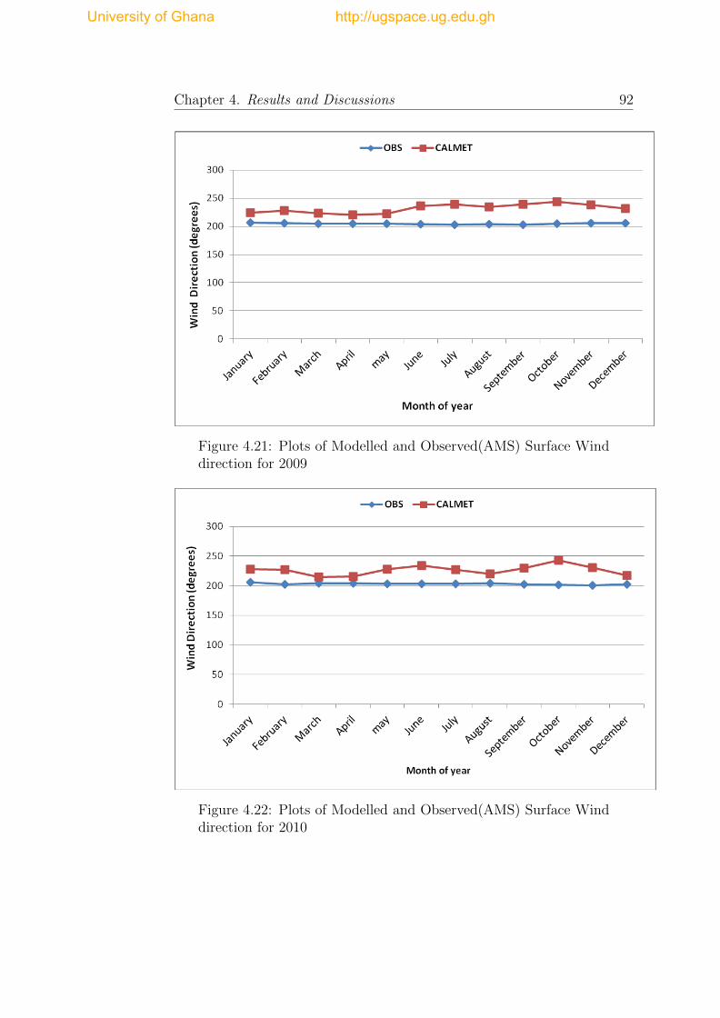
Chapter 4. Results and Discussions 92
Figure 4.21: Plots of Modelled and Observed(AMS) Surface Winddirection for 2009
Figure 4.22: Plots of Modelled and Observed(AMS) Surface Winddirection for 2010
University of Ghana http://ugspace.ug.edu.gh

Chapter 4. Results and Discussions 93
Figure 4.23: Plots of Modelled and observed(AMS) Surface Winddirection for 2011
Figure 4.24: Plots of Modelled and observed(AMS) Surface Winddirection for 2012
University of Ghana http://ugspace.ug.edu.gh

Chapter 4. Results and Discussions 94
Figure 4.25: Plots of Modelled and observed(AMS) Surface Winddirection for 2013
Figure 4.26: Plots of Modelled and Observed(TMS) Surface Winddirection for 2008
University of Ghana http://ugspace.ug.edu.gh

Chapter 4. Results and Discussions 95
Figure 4.27: Plots of Modelled and Observed(TMS) Surface Winddirection for 2009
Figure 4.28: Plots of Modelled and Observed(TMS) Surface Winddirection for 2010
University of Ghana http://ugspace.ug.edu.gh

Chapter 4. Results and Discussions 96
Figure 4.29: Plots of Modelled and observed(TMS) Surface Winddirection for 2011
Figure 4.30: Plots of Modelled and observed(TMS) Surface Winddirection for 2012
University of Ghana http://ugspace.ug.edu.gh

Chapter 4. Results and Discussions 97
Figure 4.31: Plots of Modelled and observed(TMS) Surface Winddirection for 2013
was found for 2012. Generally, R values for wind direction were lower
between model and observed data from both stations.
NMSE values were encouragingly low for wind direction for both stations
(0.01 - 0.2) reflecting a low scatter in the entire data set. However, nmse
values obtained for speed for AMS were high (0.88 - 1.4) indicating a large
scatter in the speed data. NMSE value for speed for TMS were satisfactory
(0.1 - 0.24).
IOA between modelled and observed data for all the years was above 0.60
for both variables from both stations except for 2011 speeds.
The negative FB values for direction are indicative of the overpredictions
University of Ghana http://ugspace.ug.edu.gh

Chapter 4. Results and Discussions 98
by CALMET of the observed wind direction from both meteorological sta-
tions as shown in Figs.4.20 - 4.25 for AMS and Figs.4.26 - 4.31 for TMS.
CALMET clearly under-predicts observed speeds as is seen in the positive
FB values. Whiles CALMET overpredicts surface wind direction, it under-
estimates wind speeds as shown in Figs.4.32 - 4.37 for AMS and Figs.4.38
- 4.43 for TMS.
Figure 4.32: Plots of Modelled and Observed(AMS) Surface WindSpeed for 2008
University of Ghana http://ugspace.ug.edu.gh

Chapter 4. Results and Discussions 99
Figure 4.33: Plots of Modelled and Observed(AMS) Surface WindSpeed for 2009
Figure 4.34: Plots of Modelled and Observed(AMS) Surface WindSpeed for 2010
University of Ghana http://ugspace.ug.edu.gh

Chapter 4. Results and Discussions 100
Figure 4.35: Plots of Modelled and Observed(AMS) Surface WindSpeed for 2011
Figure 4.36: Plots of Modelled and Observed(AMS) Surface WindSpeed for 2012
University of Ghana http://ugspace.ug.edu.gh

Chapter 4. Results and Discussions 101
Figure 4.37: Plots of Modelled and Observed(AMS) Surface WindSpeed for 2013
University of Ghana http://ugspace.ug.edu.gh

Chapter 4. Results and Discussions 102
Figure 4.38: Plots of Modelled and Observed(TMS) Surface WindSpeed for 2008
These challenges can be attributed to the quality of the initial winds. The
quality of the initial wind fields of the diagnostic model (from WRF) is of
vital importance for the resultant wind fields. While CALMET is able to
add value to even 5 km WRF fields, a resolution reduction of WRF to 10
km grid spacing induces errors with respect to unresolved air flows which
CALMET is unable to correct in most cases (Truhetz et al., 2007).
These statistical measures, generally, suggest a good performance of CAL-
MET .
University of Ghana http://ugspace.ug.edu.gh

Chapter 4. Results and Discussions 103
Figure 4.39: Plots of Modelled and Observed(TMS) Surface WindSpeed for 2009
Figure 4.40: Plots of Modelled and Observed(TMS) Surface WindSpeed for 2010
University of Ghana http://ugspace.ug.edu.gh

Chapter 4. Results and Discussions 104
Figure 4.41: Plots of Modelled and Observed(TMS) Surface WindSpeed for 2011
Figure 4.42: Plots of Modelled and Observed(TMS) Surface WindSpeed for 2012
University of Ghana http://ugspace.ug.edu.gh

Chapter 4. Results and Discussions 105
Figure 4.43: Plots of Modelled and Observed(TMS) Surface WindSpeed for 2013
4.6 Spatial Distribution of Emissions
Concentrations contours of annual averages of the modelled emissions for
the 6-year period are presented in Figs.4.44 - 4.46. The plots reflect the
spread of the pollutants and also shows the likely wind direction preva-
lent in the study area for 2008. The spread of the SO2 plume is larger
due to its high diffusivity and low density compared with NO2 and PM2.5.
Consequently, it impacts a larger part of the study area with maximum
contours of 610 µg/m3 near the souce of emission and minimum contours
of 10 µg/m3. Due to the predominant south westerly winds of the year
University of Ghana http://ugspace.ug.edu.gh

Chapter 4. Results and Discussions 106
Figure 4.44: 2008 Annual Average Concentration contours of SO2
in the Study Area
(windrose shown earlier), receptors located upwind are the most hit. Ac-
cording to Chan and Kwok (2000), fine and especially ultra-fine particles
are expected to disperse in the air like gases. The larger-sized particles,
however, are greatly affected by gravity and thus have a shorter residence
time in the air. This explains the fairly elevated PM2.5 levels.
Even though the emission rates for 2009 is similar to that of 2008, the
concentration contours of pollutants are lower with maximum SO2, NO2
and PM2.5 contours of 75 µg/m3, 72 µg/m3 and 62 µg/m3 respectively
as shown in Figs.4.47, 4.48 and 4.49 respectively. Since emission rates
are assumed to be constant, the differences could be attributed mainly to
University of Ghana http://ugspace.ug.edu.gh

Chapter 4. Results and Discussions 107
Figure 4.45: 2008 Annual Average Concentration contours of NO2
in the Study Area
meteorological conditions. The wind rose for 2009 is shown in Fig.4.50.
The predominant south westerly winds of the year represent 90% of total
winds. Wind speed class of 3.3-5.4 m/s constitutes 73% followed by 22% of
speeds between 5.4 - 8.5 m/s and 3% of total winds falling into class 1.8 -
3.3 m/s . Total calm winds are nil. A comparison of wind roses for 2009 and
2008 shows that the average wind speed was higher in 2009 than in 2008.
Strong winds tend to increase pollutant mixing and dispersion and hence
decreasing ground level concentrations. The year 2008 experienced more
low wind speeds and calm periods. This meteorological condition favours
increased ground level concentrations of pollutants as evidenced by the
2008 contour plots. Low synoptic winds create a well-known meteorological
University of Ghana http://ugspace.ug.edu.gh

Chapter 4. Results and Discussions 108
Figure 4.46: 2008 Annual Average Concentration contours of PM2.5
in the Study Area
situation that favours air pollution built-up in urban areas (Jones et al.,
2000, Qin and Kot, 1993).
Figs.4.51 - 4.53 present concentration contours of the pollutants for 2010
with its accompanying wind rose in Fig. 4.54. Emission rate of the pol-
lutants for 2010 was the highest. However, the positive influence of the
prevailing winds for the year was seen in the generally low concentrations
similar to those in 2009. The statistics of the 2010 surface winds are quite
University of Ghana http://ugspace.ug.edu.gh

Chapter 4. Results and Discussions 109
Figure 4.47: 2009 Annual Average Concentration contours of SO2
in the Study Area
similar with 2009 winds.
Concentration contours for the remaining years and their corresponding
windroses are shown by Figs. 4.55 - 4.66.
Figure 4.66: Wind Rose Depicting 2013 Surface Winds in the Studyarea
It can be seen from Fig. 4.58, Fig.4.62 and Fig. 4.66 that the percentage of
the upper wind speed class, 5.4 - 8.5 m/s, of total winds decreased giving
rise to an increase in low speed percentages. Infact, 2013 recorded a low
University of Ghana http://ugspace.ug.edu.gh

Chapter 4. Results and Discussions 110
Figure 4.48: 2009 Annual Average Concentration contours of NO2
in the Study Area
Figure 4.49: 2009 Annual Average Concentration contours of PM2.5
in the Study Area
University of Ghana http://ugspace.ug.edu.gh

Chapter 4. Results and Discussions 111
Figure 4.50: Wind Rose Depicting 2009 Surface Winds in the Studyarea
speed class (1.8 - 33) m/s of about 18%. Low wind speed conditions are typ-
ically associated with the worst air pollution episodes in cities (Di Sabatino
et al., 2003). Therefore, predicted concentrations at the various receptors
should have been higher for 2011 - 2013. This, however, was not observed.
It should be recalled that emission rates from the refinery saw a steady
decline from 2011 to 2013 as a result of shortfalls in crude supply. This
is the reason for the low concentration contours observed within the study
area.
University of Ghana http://ugspace.ug.edu.gh

Chapter 4. Results and Discussions 112
Figure 4.51: 2010 Annual Average Concentration contours of SO2
in the Study Area
4.7 Interannual Predicted Concentrations of
Emissions at Receptors
As was mentioned earlier in this chapter, receptors located within 10 - 15
km of the refinery are the most impacted by the refinery emissions. For this
reason, this subsection takes another look at the annual variations in the
modelled daily average pollutant concentrations at these receptors using
the different emission rates estimated for the years under consideration.
Results of this investigation are presented in Figs. 4.67, 4.68 and 4.69. The
plots reflect the year-to-year variability in weather conditions.
University of Ghana http://ugspace.ug.edu.gh

Chapter 4. Results and Discussions 113
Figure 4.52: 2010 Annual Average Concentration contours of NO2
in the Study Area
Figure 4.53: 2010 Annual Average Concentration contours of PM2.5
in the Study Area
University of Ghana http://ugspace.ug.edu.gh

Chapter 4. Results and Discussions 114
Figure 4.54: Wind Rose Depicting 2010 Surface Winds in the Studyarea
A look at Fig. 4.67 reveals that the highest daily SO2 concentration occured
at Tema Steelworks area followed by Tema Comm 25 for all the years. Con-
centrations at the Tema Steelworks area for years ranged from about 220
- 280 µg/m3 with 2010 concentrations being the highest. Concentrations
at Tema Comm 25 ranged between 60 - 100 µg/m3 with the highest occur-
ing in 2010. Other receptors recording concentrations above 50 µg/m3 are
Ashiaman and Sebrepor. The other receptors showed concentrations lower
than 50 µg/m3 except the Tema General Hospital which recorded about
70 µg/m3 in 2013. Comparing these concentration values with WHO daily
average guideline of 125 µg/m3 for SO2 (WHO (2000)), it is obvious that
University of Ghana http://ugspace.ug.edu.gh

Chapter 4. Results and Discussions 115
Figure 4.55: 2011 Annual Average Concentration contours of SO2
in the Study Area
Figure 4.56: 2011 Annual Average Concentration contours of NO2
in the Study Area
University of Ghana http://ugspace.ug.edu.gh

Chapter 4. Results and Discussions 116
Figure 4.57: 2011 Annual Average Concentration contours of PM2.5
in the Study Area
concentrations at the Tema Steelworks area well exceeded the regulatory
limit. These concentrations also exceeded the Ghana EPA guideline values
of 150 µg/m3 for industrial areas and 100 µg/m3 for residential areas.
From Fig. 4.68, maximum NO2 concentration of about 78 µg/m3 occured
again at the Tema Steelworks after which TOR, Tema Comm 25 and Tema
General Hospital follow. A comparison of the concentrations at the recep-
tors with the WHO guideline value for NO2 (50 µg/m3) and the Ghana
EPA values of 60 µg/m3 for residential and 150 µg/m3 for industrial areas,
it can be concluded concentrations fall below these regulatory limits except
the Tema Steelworks area. As far as the Ghana guideline values are con-
cerned, the conclusion can be made that the refinery is not polluting the
University of Ghana http://ugspace.ug.edu.gh
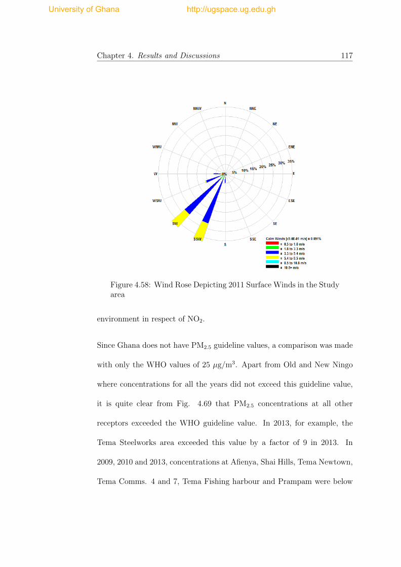
Chapter 4. Results and Discussions 117
Figure 4.58: Wind Rose Depicting 2011 Surface Winds in the Studyarea
environment in respect of NO2.
Since Ghana does not have PM2.5 guideline values, a comparison was made
with only the WHO values of 25 µg/m3. Apart from Old and New Ningo
where concentrations for all the years did not exceed this guideline value,
it is quite clear from Fig. 4.69 that PM2.5 concentrations at all other
receptors exceeded the WHO guideline value. In 2013, for example, the
Tema Steelworks area exceeded this value by a factor of 9 in 2013. In
2009, 2010 and 2013, concentrations at Afienya, Shai Hills, Tema Newtown,
Tema Comms. 4 and 7, Tema Fishing harbour and Prampam were below
University of Ghana http://ugspace.ug.edu.gh

Chapter 4. Results and Discussions 118
Figure 4.59: 2012 Annual Average Concentration contours of SO2
in the Study Area
Figure 4.60: 2012 Annual Average Concentration contours of NO2
in the Study Area
University of Ghana http://ugspace.ug.edu.gh

Chapter 4. Results and Discussions 119
Figure 4.61: 2012 Annual Average Concentration contours of PM2.5
in the Study Area
this guideline value. Generally, however, it is quite obvious that PM2.5
pollution by the refinery is substantial.
4.8 Seasonal Variation of Pollutants
Results of seasonal variability investigations are presented in monthly aver-
age concentration plots of pollutants in 2013 at Tema Steelworks and Tema
Comm. 25, Kpone and the Tema General hospital as seen in Figs. 4.70 -
4.73. Predicted monthly concentrations of the pollutants for the entire year
show that highest values occured in August at Tema Steelworks and Tema
Comm 25. At Kpone, highest values occured in October and in December
University of Ghana http://ugspace.ug.edu.gh

Chapter 4. Results and Discussions 120
Figure 4.62: Wind Rose Depicting 2012 Surface Winds in the Studyarea
at the hospital. Further, it can be seen that, generally, the second half of
the year during which the dry season occurs, shows slightly higher concen-
trations than the first half. The major wet season in the first half of the
year (April-June) could be responsible for the lower concentrations of the
pollutants. The effect of precipitation on atmospheric pollutants are well
researched (Aleksandropoulou and Lazaridis, 2004, Davies, 1976, Pandey
et al., 1992, Ravindra et al., 2003).
A particular factor that can affect pollutant distribution is the type of sta-
bility condition which is a function of temperature. During the dry and
warmer months of January, February and March, the atmosphere is more
University of Ghana http://ugspace.ug.edu.gh

Chapter 4. Results and Discussions 121
Figure 4.63: 2013 Annual Average Concentration contours of SO2
in the Study Area
Figure 4.64: 2013 Annual Average Concentration contours of NO2
in the Study Area
University of Ghana http://ugspace.ug.edu.gh

Chapter 4. Results and Discussions 122
Figure 4.67: Daily Average SO2 Concentrations at various receptors
Figure 4.68: Daily Average NO2 Concentrations at various recep-tors
unstable because of the elevated temperatures. This increases the level of
turbulence, which, in turn, increases the dispersive capability of the atmo-
sphere. As a consequence, pollutants disperse relatively rapidly in both the
horizontal and vertical directions, and its ground level concentration decays
over relatively short distances. The atmosphere is more stable during the
cooler months of July and August due to the slightly reduced temperatures
University of Ghana http://ugspace.ug.edu.gh

Chapter 4. Results and Discussions 123
Figure 4.69: Daily Average PM2.5 Concentration at various recep-tors
causing a reduction in the dispersive ability of the atmosphere. As a result,
ground level concentrations of pollutants could increase as seen generally
in Figs. 4.70 - 4.73. A plot showing the monthly variation of temperature
over the years around the refinery is shown in Fig. 4.74.
University of Ghana http://ugspace.ug.edu.gh

Chapter 4. Results and Discussions 124
Figure 4.70: 2013 Monthly Average concentrations of pollutants atTema Steelworks
Figure 4.71: 2013 Monthly Average concentrations of pollutants atTema Comm. 25
University of Ghana http://ugspace.ug.edu.gh

Chapter 4. Results and Discussions 125
Figure 4.72: 2013 Monthly Average concentrations of pollutants atKpone
Figure 4.73: 2013 Monthly Average concentrations of pollutants atTema Gen. Hosp
University of Ghana http://ugspace.ug.edu.gh
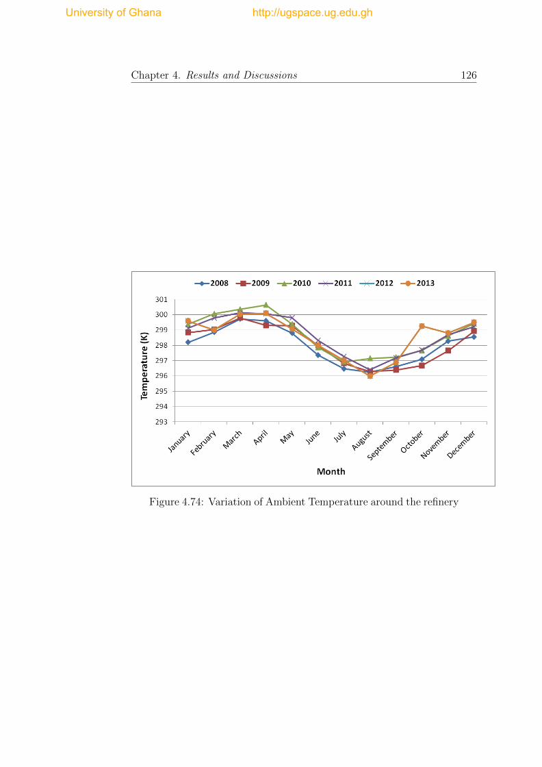
Chapter 4. Results and Discussions 126
Figure 4.74: Variation of Ambient Temperature around the refinery
University of Ghana http://ugspace.ug.edu.gh

Chapter 5
Conclusions and
Recommendations
5.1 Introduction
The overriding purpose of this study was to simulate the dispersion and
transport of pollutants emitted during the processing of crude oil by TOR,
in the Greater Accra Region of Ghana using the California Puff (CALPUFF)
modeling system. To accomplish this goal, it became necessary to reach
some prerequisite goals. The importance of air quality models in under-
standing air pollution and their effects was emphazised during the literature
review conducted for this dissertation. Subsequent to this, it was neces-
sary to estimate daily average emission rates from the refinery for the years
under review as an important input for CALPUFF. The WRF model was
127
University of Ghana http://ugspace.ug.edu.gh

Chapter 5. Conclusions and Recommendations 128
run to generate the initial meteorological data necessary to initialize CAL-
MET model and to drive the dispersion model, CALPUFF. To validate
the CALPUFF modelling system, comparisons were made between some
measured and modelled data. Once these prerequisite goals were achieved,
the main purpose of the research was realised. This chapter reports the
conclusions and recommendations that resulted from this study.
5.1.1 Conclusions
The mass balance approach, which was employed to estimate the refinery
pollutant emissions revealed that total CO2 emissions were the highest,
peaking in 2008 and followed by VOCs. Particulate matter rates were ob-
served to be fairly constant over the years under review. The SO2 and
NO2 emission rates were next with NO2 being the least. A steady decline
in emissions was observed over the years as a result of the reduction in
production due to the frequent shortfalls in the refinery’s crude oil sup-
ply consequently leading virtually to a halt in refinery operations in 2014
preceded by intermittent shutdowns.
To determine the radius of impact of the refinery emissions, the dispersion
of SO2, NO2 and PM was modelled over a space of 60 km2 centred nearly
around the refinery was carried out. Within this space, receptor locations
representing residential and health facilities, schools and industries were
University of Ghana http://ugspace.ug.edu.gh

Chapter 5. Conclusions and Recommendations 129
identified and the maximum daily average concentrations of the pollutants
at these location calculated using the CALPUFF. Meteorological data used
to drive CALMET, the meteorological model, was generated by running
WRF. It was concluded, based on the preliminary simulation results, that
the impact of the refinery emissions was felt at receptor locations within a
radius of about 20 km around the refinery. Furthermore, receptors located
on the north and north-eastern parts of the refinery showed relatively higher
pollutant concentrations than other parts of the study domain as a result of
the predominant south-westerly winds in the study area. Conversely, south-
western receptors were the least impacted by refinery emissions. A check
with ambient pollutant guidelines of WHO and EPA Ghana showed that the
concentrations of SO2 and NO2 at 36 receptors did not exceed regulatory
limits. Two receptors, however, exceeded regulatory limits. Ground level
concentrations of PM, however, exceeded the regulatory limits at almost
all receptors.
In order to validate the modelling system, results of the meteorological
and dispersion simulation were compared with measurements and observa-
tions using statistical measures. The statistical measures revealed a good
agreement between model and observations leading to the conclusion that
CALPUFF can be used satisfactorily for air pollution studies and for check-
ing compliance of industrial set-ups with standards.
University of Ghana http://ugspace.ug.edu.gh

Chapter 5. Conclusions and Recommendations 130
It should be highlighted that the utilization of CALPUFF for the sim-
ulation of dispersion of refinery emissions and for the description of air
quality issues over the Tema Metropolitan Area and parts of the Accra
Metropolitan area represents a useful instrument that may contribute to
the establishment of environmental managing policies and to regulatory
purposes.
Even though the CALPUFF modelling system has been used to successfully
simulate the dispersion of refinery emissions, it is not without limitations for
developing countries. The major limitation is related to the meteorological
data requirements of CALMET. Calmet has switches for the use of either
observations or meteorological data from a numerical weather prediction
model or a combination of both, which is usually preferred. However, when
observations (surface and upper air) are to be used, hourly to 3-hourly data
is required. This specification of data is not available in most developing
countries hence limiting its use. For example, the Ghana meteorological
service could provide daily surface data and not upper air data.
5.1.2 Recommendations
The following recommendations are offered for related research and relevant
institutions:
University of Ghana http://ugspace.ug.edu.gh

Chapter 5. Conclusions and Recommendations 131
1. Even though the refinery emissions in almost all the receptors do not
generally exceed regulatory limits, it is obvious that the inclusion of
all emittors in the model will result in increased levels of pollutants
which could have serious health implications on the exposed popula-
tion. To be able to quantify the contributions of the other emittors
within the industrial complex, their emission rates are necessary. This
can be obtained through an emissions inventory campaign within the
Tema Industrial area by EPA, Ghana in collaboration with all the in-
dustries. Closely linked to this, emission factors for various pollutants
can also be developed.
2. The effects of refinery emissions on critical receptors, receptors lo-
cated in the immediate north and north east of the refinery should be
investigated through a health assessment to determine which diseases
affect the populations in these receptors.
3. Despite the serious health and environmental implications of popula-
tion exposure to VOCs and their strong association with ozone (O3),
their dispersion and transport could not be modelled. This is be-
cause of its composite nature. CALPUFF models single entities and
not composites. It is therefore recommended that further research be
carried out to characterise the VOCs for modelling purposes.
University of Ghana http://ugspace.ug.edu.gh

Chapter 5. Conclusions and Recommendations 132
4. SO2 and NO2 are easily transformed into sulphates and nitrates in the
atmosphere which are implicated in many environmental challenges
and would therefore be interesting to look at closely. The effect of
chemical transformation of these pollutants can be investigated using
the mesopuff module in CALPUFF.
5. Real time applications using CALPUFF is recommended as this will
be useful in real time analysis and prediction of plume transport and
diffusion during accidental releases.
6. Since results of this research clearly indicates PM2.5 pollution from
TOR, it is important that EPA Ghana conducts regular monitoring
exercises at all industries in order to enforce compliance to guidelines.
7. To reduce the error associated with emission rates input into air qual-
ity models, it is essential to use data from measurements made di-
rectly from the point source. It is therefore recommended that TOR
puts in measures to ensure that flow meters are installed at various
exit points.
University of Ghana http://ugspace.ug.edu.gh

References 133
References
Abdul-Wahab, S. A. (2003). SO2 dispersion and monthly evaluation of the
industrial source complex short-term (ISCST32) model at Mina Al-Fahal
refinery, Sultanate of Oman. Environmental management, 31(2):0276–
0291.
Addo, K. A. (2013). Shoreline morphological changes and the human factor.
Case study of Accra, Ghana. Journal of Coastal Conservation, 17(1):85–
91.
Affum, H., Oduro-Afriyie, K., Nartey, V., Adomako, D., and Nyarko, B. B.
(2008). Biomonitoring of airborne heavy metals along a major road in
Accra, Ghana. Environmental monitoring and assessment, 137(1-3):15–
24.
Ahuja, S. (1996). Evaluation of MESOPUFF-II-SOx Transport and Depo-
sition in the Great Lakes Region. PhD thesis, University of Toledo.
Al-Fadhli, F. M., Kimura, Y., McDonald-Buller, E. C., and Allen, D. T.
(2011). Impact of flare destruction efficiency and products of incom-
plete combustion on ozone formation in Houston, Texas. Industrial &
Engineering Chemistry Research, 51(39):12663–12673.
Aleksandropoulou, V. and Lazaridis, M. (2004). Spatial distribution of
gaseous and particulate matter emissions in Greece. Water, air, and soil
pollution, 153(1-4):15–34.
Arku, R. E., Vallarino, J., Dionisio, K. L., Willis, R., Choi, H., Wilson,
J. G., Hemphill, C., Agyei-Mensah, S., Spengler, J. D., and Ezzati, M.
(2008). Characterizing air pollution in two low-income neighborhoods in
Accra, Ghana. Science of the total environment, 402(2):217–231.
University of Ghana http://ugspace.ug.edu.gh

References 134
Bansah, K. J. and Amegbey, N. (2012). Ambient Particulate Matter
Monitoring-A Case Study at Tarkwa. Research Journal of Environmental
and Earth Sciences, 4(4):419–423.
Boubel, R. W., Vallero, D., Fox, D. L., Turner, B., and Stern, A. C. (2013).
Fundamentals of air pollution, pages 291–320. Elsevier.
Briggs, G. A. (1975). Plume rise predictions, lectures on air pollution and
environment impact analysis. Am. Meteorol. Soc., Boston, USA, 10.
Britter, R. and Hanna, S. (2003). Flow and dispersion in urban areas.
Annual Review of Fluid Mechanics, 35(1):469–496.
Brown, R. A. (1991). Fluid Mechanics of the Atmosphere, volume 47, pages
197–206. Academic Press.
Brunekreef, B. and Holgate, S. T. (2002). Air pollution and health. The
lancet, 360(9341):1233–1242.
Chan, L. and Kwok, W. (2000). Vertical Dispersion of Suspended Par-
ticulates in urban area of Hong Kong. Atmospheric Environment,
34(26):4403–4412.
Chandrasekar, A., Philbrick, C. R., Clark, R., Doddridge, B., and Geor-
gopoulos, P. (2003). Evaluating the performance of a computationally
efficient MM5/CALMET system for developing wind field inputs to air
quality models. Atmospheric Environment, 37(23):3267–3276.
Cimorelli, A. J. et al. (1998). AERMOD–Description of model formulation.
Collett, R. S. and Oduyemi, K. (1997). Air quality modelling: a tech-
nical review of mathematical approaches. Meteorological Applications,
4(03):235–246.
University of Ghana http://ugspace.ug.edu.gh

References 135
Corma, A., Palomares, A., Rey, F., and Marquez, F. (1997). Simultaneous
Catalytic Removal of SOx and NOx with Hydrotalcite-Derived Mixed
Oxides Containing Copper, and Their Possibilities to Be Used in FCC
Units. Journal of catalysis, 170(1):140–149.
Darko, E. and Quist, M. (2012). Low Sulphur Diesel and Refining Process,
Technical and Financial Implications for Tema Oil Refinery (TOR) Lim-
ited. In Workshop organized by National Petroleum Authority in Part-
nership for Clean fuels and Vehicles under the auspices of United Nation
Environmental Programme (UNEP) in Accra, Ghana from September
13-14, 2012.
Davies, T. (1976). Precipitation Scavenging of Sulphur Dioxide in an In-
dustrial Area. Atmospheric Environment (1967), 10(10):879–890.
de Leeuw, F. A., Moussiopoulos, N., Sahm, P., and Bartonova, A. (2001).
Urban Air Quality in Larger Conurbations in the European Union. En-
vironmental Modelling & Software, 16(4):399–414.
Demuzere, M., Trigo, R., Vila-Guerau de Arellano, J., and Van Lipzig,
N. (2009). The impact of weather and atmospheric circulation on o3
and pm10 levels at a rural mid-latitude site. Atmospheric Chemistry and
Physics, 9(8):2695–2714.
Di Sabatino, S., Kastner-Klein, P., Berkowicz, R., Britter, R., and Fe-
dorovich, E. (2003). The modelling of turbulence from traffic in urban
dispersion modelspart i: theoretical considerations. Environmental Fluid
Mechanics, 3(2):129–143.
Dios, M., Souto, J., and Casares, J. (2013). Experimental development of
CO2, SO2 and NO emission factors for mixed lignite and sub-bituminous
coal-fired power plant. Energy, 53:40–51.
University of Ghana http://ugspace.ug.edu.gh

References 136
Dresser, A. L. and Huizer, R. D. (2011). CALPUFF and AERMOD model
validation study in the near field: Martins Creek revisited. Journal of
the Air & Waste Management Association, 61(6):647–659.
EIPPCB (2012). Best Available Techniques (BAT) Reference Document
for the Refining of Mineral Oil and Gas. Technical report.
England, G. C., Zielinska, B., Loos, K., Crane, I., and Ritter, K. (2000).
Characterizing PM2.5 emission profiles for stationary sources: compar-
ison of traditional and dilution sampling techniques. Fuel Processing
Technology, 65:177–188.
Fenger, J. (1999). Urban air quality. Atmospheric environment,
33(29):4877–4900.
Fernando, H. (2010). Fluid dynamics of urban atmospheres in complex
terrain. Annual Review of Fluid Mechanics, 42:365–389.
Ferretti, M., Andrei, S., Caldini, G., Grechi, D., Mazzali, C., Galanti, E.,
and Pellegrini, M. (2008). Integrating monitoring networks to obtain esti-
mates of ground-level ozone concentrationsA proof of concept in Tuscany
(central Italy). Science of the Total Environment, 396(2):180–192.
Fishwick, S. and Scorgie, Y. (2011). Performance of CALPUFF in predict-
ing time-resolved particulate matter concentrations from a large scale
surface mining operation. In Proceedings of CASANZ Conference from
30 July2 August,2011, Auckland, pages 647–659.
Fowler, D., Pilegaard, K., Sutton, M., Ambus, P., Raivonen, M., Duyzer,
J., Simpson, D., Fagerli, H., Fuzzi, S., Schjørring, J. K., et al. (2009).
Atmospheric composition change: ecosystems–atmosphere interactions.
Atmospheric Environment, 43(33):5193–5267.
University of Ghana http://ugspace.ug.edu.gh

References 137
Ghannam, K. and El-Fadel, M. (2013). Emissions characterization
and regulatory compliance at an industrial complex: an integrated
MM5/CALPUFF approach. Atmospheric Environment, 69:156–169.
G.S.S (2012). 2010 Population & Housing Census of Ghana: GA-MY,
page 5. Ghana Statistical Service.
Guilbert, J. et al. (2003). The World Health Report 2002-reducing Risks,
promoting healthy life. Education for health-Abingdon-Carfax Publishing
Limited, 16(2):230–230.
Hanna, S., Chang, J., and Strimaitis, D. (1993). Hazardous gas model
evaluation with field observations. Atmospheric Environment. Part A.
General Topics, 27(15):2265–2285.
Hanna, S. R., Strimaitis, D. G., and Chang, J. C. (1991). Evaluation of
fourteen hazardous gas models with ammonia and hydrogen fluoride field
data. Journal of hazardous materials, 26(2):127–158.
Hansard, R., Maher, B., and Kinnersley, R. (2011). Biomagnetic monitor-
ing of industry-derived particulate pollution. Environmental Pollution,
159(6):1673–1681.
Harding, R., Peters, A., and Nee, J. (2001). New developments in fcc
catalyst technology. Applied Catalysis A: General, 221(1):389–396.
Hernandez, A., Saavedra, S., Rodrıguez, A., Souto, J. A., and Casares,
J. J. (2014). Coupling WRF and CALMET models: Validation during
primary pollutants glc episodes in an Atlantic coastal region. In Air
Pollution Modeling and its Application XXII, pages 681–684. Springer.
Hildemann, L. M., Klinedinst, D. B., Klouda, G. A., Currie, L. A., and
Cass, G. R. (1994). Sources of urban contemporary carbon aerosol. En-
vironmental science & technology, 28(9):1565–1576.
University of Ghana http://ugspace.ug.edu.gh

References 138
Holmes, N. S. and Morawska, L. (2006). A review of dispersion modelling
and its application to the dispersion of particles: an overview of differ-
ent dispersion models available. Atmospheric Environment, 40(30):5902–
5928.
Holnicki, P. (2011). Uncertainty in integrated modelling of air quality.
Holtslag, A. and Van Ulden, A. (1983). A simple scheme for daytime
estimates of the surface fluxes from routine weather data. Journal of
Climate and Applied Meteorology, 22(4):517–529.
Irwin, J. S. (1983). Estimating plume dispersion-a comparison of several
sigma schemes. Journal of Climate and Applied Meteorology, 22(1):92–
114.
Jackson, P. (1981). On the displacement height in the logarithmic velocity
profile. Journal of Fluid Mechanics, 111:15–25.
Janjic, Z. (2003). A nonhydrostatic model based on a new approach. Me-
teorology and Atmospheric Physics, 82(1-4):271–285.
Janjic, Z. I. (2002). Nonsingular implementation of the mellor–yamada
level 2.5 scheme in the ncep meso model. NCEP office note, 437:61.
Jimenez-Garcıa, G., Aguilar-Lopez, R., and Maya-Yescas, R. (2011). The
fluidized-bed catalytic cracking unit building its future environment.
Fuel, 90(12):3531–3541.
Jones, S., Fisher, B. E., Gonzalez-Flesca, N., and Sokhi, R. (2000). The use
of measurement programmes and models to assess concentrations next to
major roads in urban areas. Environmental Monitoring and Assessment,
64(2):531–547.
Khamsimak, P., Koonaphapdeelert, S., and Tippayawong, N. (2012). Sim-
ulated Effect of Terrain Change on Dispersion of SO2 Emission Around
University of Ghana http://ugspace.ug.edu.gh
References 139
Mae Moh Basin. Recent Advances in Energy,Environment and Economic
Development, pages 200–204.
Kumar, A., Luo, J., and Bennett, G. F. (1993). Statistical evaluation of
lower flammability distance (lfd) using four hazardous release models.
Process Safety Progress, 12(1):1–11.
Levy, J. I., Wilson, A. M., Evans, J. S., and Spengler, J. D. (2003).
Estimation of primary and secondary particulate matter intake frac-
tions for power plants in Georgia. Environmental science & technology,
37(24):5528–5536.
Liu, M.-K. and Yocke, M. A. (1980). Siting of wind turbine generators in
complex terrain. Journal of Energy, 4(1):10–16.
Macdonald, R. (2000). Modelling the mean velocity profile in the urban
canopy layer. Boundary-Layer Meteorology, 97(1):25–45.
Martın, J., Lumbreras, J., and Rodrıguez, M. (2003). Testing flare emission
factors for flaring in refineries. In US EPA 12th International emissions
inventory conference, San Diego.
Martin, R. V. (2008). Satellite remote sensing of surface air quality. Atmo-
spheric Environment, 42(34):7823–7843.
Maya-Yescas, R., Villafuerte-Macıas, E., Aguilar, R., and Salazar-Sotelo,
D. (2005). Sulphur oxides emission during fluidised-bed catalytic crack-
ing. Chemical Engineering Journal, 106(2):145–152.
Michalakes, J., Dudhia, J., Gill, D., Henderson, T., Klemp, J., Skamarock,
W., and Wang, W. (2004). The Weather Research and Forecast Model:
Software Architecture and Performance. In Proceedings of the 11th
ECMWF Workshop on the Use of High Performance Computing In Me-
teorology, volume 25, page 29. World Scientific.
University of Ghana http://ugspace.ug.edu.gh

References 140
Monin, A. and Obukhov, A. (1954). Basic laws of turbulent mixing in
the surface layer of the atmosphere. Contrib. Geophys. Inst. Acad. Sci.
USSR, 151:163–187.
Muff, R. and Efa, E. (2006). Ghana-Germany technical cooperation project:
environmental and engineering geology for urban planning in the Accra-
Tema area. Explanatory notes for the geological map for urban planning,
1(50):000.
Muller, N. Z. and Mendelsohn, R. (2007). Measuring the damages of air
pollution in the united states. Journal of Environmental Economics and
Management, 54(1):1–14.
Ofosu, F. G., Hopke, P. K., Aboh, I. J., and Bamford, S. A. (2012). Char-
acterization of fine particulate sources at Ashaiman in Greater Accra,
Ghana. Atmospheric Pollution Research, 3(3).
Pandey, J., Agrawal, M., Khanam, N., Narayan, D., and Rao, D. (1992). Air
pollutant concentrations in Varanasi, India. Atmospheric Environment.
Part B. Urban Atmosphere, 26(1):91–98.
Pasquill, F. and Smith, F. (1983). Atmospheric diffusion.: Study of the dis-
persion of windborne material from industrial and other sources. JOHN
WILEY & SONS, 605 THIRD AVE., NEW YORK, NY 10016, USA.
1983.
Pearce, J. L., Beringer, J., Nicholls, N., Hyndman, R. J., Uotila, P., and
Tapper, N. J. (2011). Investigating the influence of synoptic-scale meteo-
rology on air quality using self-organizing maps and generalized additive
modelling. Atmospheric Environment, 45(1):128–136.
University of Ghana http://ugspace.ug.edu.gh

References 141
Perez Ballesta, P., Field, R., Fernandez-Patier, R., Galan Madruga, D.,
Connolly, R., Baeza Caracena, A., and De Saeger, E. (2008). An ap-
proach for the evaluation of exposure patterns of urban populations to
air pollution. Atmospheric Environment, 42(21):5350–5364.
Products, U. O. (1997). Fluid catalytic cracking process manual - process
calculations,. pages 21–33, 64–68.
Protonotariou, A., Bossioli, E., Athanasopoulou, E., Dandou, A., Tombrou,
M., Assimakopopoulos, V., Flocas, H., and Chelmis, C. (2004). Valida-
tion and inter-comparison of CALPUFF regulatory model to Eulerian
models and measurements. An application over the greater Athens area,
Greece. In Proceedings of the 9th International Conference on Harmoni-
sation within Atmospheric Dispersion Modelling for Regulatory Purposes,
pages 131–135.
Puliafito, S. E., Allende, D., Fernandez, R., Castro, F., and Cremades, P.
(2011). New approaches for urban and regional air pollution modelling
and management. Air Pollution/Book, 1.
Qin, Y. and Kot, S. (1993). Dispersion of vehicular emission in street
canyons, Guangzhou City, South China (PRC). Atmospheric Environ-
ment. Part B. Urban Atmosphere, 27(3):283–291.
Raupach, M. and Thom, A. S. (1981). Turbulence in and above plant
canopies. Annual Review of Fluid Mechanics, 13(1):97–129.
Ravindra, K., Mor, S., Kamyotra, J., Kaushik, C., et al. (2003). Variation
in spatial pattern of criteria air pollutants before and during initial rain
of monsoon. Environmental monitoring and assessment, 87(2):145–153.
Rotach, M. (1994). Determination of the zero plane displacement in an
urban environment. Boundary-Layer Meteorology, 67(1-2):187–193.
University of Ghana http://ugspace.ug.edu.gh

References 142
Sackey, S. S. (2012). Development of DOAS remote sensing system for
ground-based measurements of trace gas emissions in an industrial area.
PhD thesis.
Safo-Adu, G., Ofosu, F., Carboo, D., and Armah, Y. (2014). Heavy metals
and black carbon assessment of PM10 particulates along Accra–Tema
highway in Ghana. International Journal of Science and Technology,
3(8).
Schurmann, G., Algieri, A., Hedgecock, I., Manna, G., Pirrone, N., and
Sprovieri, F. (2009). Modelling local and synoptic scale influences on
ozone concentrations in a topographically complex region of Southern
Italy. Atmospheric Environment, 43(29):4424–4434.
Scire, J. S., Robe, F. R., Fernau, M. E., and Yamartino, R. J. (2000a). A
User's guide for the CALMET Meteorological Model. Earth Tech, USA,
37.
Scire, J. S., Strimaitis, D. G., and Yamartino, R. J. (2000b). A User's guide
for the CALPUFF Dispersion Model. Earth Tech, Inc, 521:1–521.
Seigneur, C., Pun, B., Pai, P., Louis, J.-F., Solomon, P., Emery, C., Morris,
R., Zahniser, M., Worsnop, D., Koutrakis, P., et al. (2000). Guidance
for the performance evaluation of three-dimensional air quality modeling
systems for particulate matter and visibility. Journal of the Air & Waste
Management Association, 50(4):588–599.
Shamarock, W., Klemp, J., Dudhia, J., Gill, D., Barker, D., Duda, M.,
Huang, X., Wang, W., and Powers, J. (2008). A Description of the
Advanced Research WRF version 3. NCAR technical note NCAR/T-
N/u2013475.
University of Ghana http://ugspace.ug.edu.gh

References 143
Skamarock, W. C., Klemp, J. B., Dudhia, J., Gill, D. O., Barker, D. M.,
Wang, W., and Powers, J. G. (2005). A description of the advanced
research wrf version 2. Technical report, DTIC Document.
Stull, R. B. (2012). An introduction to boundary layer meteorology, vol-
ume 13, page 2. Springer Science & Business Media.
Truhetz, H., Gobiet, A., and Kirchengast, G. (2007). Evaluation of a
dynamic-diagnostic modelling approach to generate highly resolved wind
fields in the Alpine region. Meteorologische Zeitschrift, 16(2):191–201.
Tsuang, B.-J. (2003). Quantification on the Source/Receptor Relationship
of Primary Pollutants and Secondary Aerosols by a Gaussian Plume Tra-
jectory Model: Part I Theory. Atmospheric Environment, 37(28):3981–
3991.
USEPA (2001). Preferred and alternative methods for estimating air emis-
sions from boilers. 2.
USEPA (2010). Available and emerging technologies for reducing green-
house gas emissions from the petroleum refining industry. 2.1.1.
USEPA (2011). Emission estimation protocol for petroleum refineries. 2.1.1.
USGS (2010). The Global Land Cover Characterization (GLCC)Database.
NCAR technical note NCAR/TN/u2013475.
Venkatesan, R., Mathiyarasu, R., and Somayaji, K. (2002). A Study of
Atmospheric Dispersion of Radionuclides at a Coastal site using a mod-
ified Gaussian Model and a Mesoscale Sea Breeze model. Atmospheric
Environment, 36(18):2933–2942.
Venkatram, A. (1978). An examination of box models for air quality sim-
ulation. Atmospheric Environment (1967), 12(12):2243–2249.
University of Ghana http://ugspace.ug.edu.gh

References 144
Versteeg, H. K. and Malalasekera, W. (2007). An Introduction to Computa-
tional Fluid Dynamics: The Finite Volume Method, pages 1–6. Pearson
Education Limited, England.
WHO (2000). Air quality guidelines for Europe, volume 91, pages 1–287.
Second Edition,Copenhagen, WHO Regional Office for Europe.
Wieringa, J. et al. (2001). New revision of davenport roughness classifica-
tion. Proc., 3EACWE, Eindhoven, The Netherlands, pages 285–292.
Willmott, C. J. (1982). Some comments on the evaluation of model per-
formance. Bulletin of the American Meteorological Society, 63(11):1309–
1313.
Wood, E. C., Herndon, S. C., Fortner, E. C., Onasch, T. B., Wormhoudt,
J., Kolb, C. E., Knighton, W. B., Lee, B. H., Zavala, M., Molina, L.,
et al. (2012). Combustion and destruction/removal efficiencies of in-use
chemical flares in the greater Houston area. Industrial & Engineering
Chemistry Research, 51(39):12685–12696.
Zadakbar, O., Vatani, A., and Karimpour, K. (2008). Flare gas recovery in
oil and gas refineries. Oil & Gas Science and Technology-Revue de l’IFP,
63(6):705–711.
Zannetti, P. (2013). Air Pollution Modeling: Theories, Computational
Methods and Available Software, pages 107–130. Springer Science & Busi-
ness Media, New York.
Zawar-Reza, P., Kingham, S., and Pearce, J. (2005). Evaluation of a year-
long dispersion modelling of PM10 using the mesoscale model TAPM
for Christchurch, New Zealand. Science of the Total Environment,
349(1):249–259.
University of Ghana http://ugspace.ug.edu.gh

References 145
Zhao, X., Peters, A., and Weatherbee, G. (1997). Nitrogen chemistry and
NOx control in a fluid catalytic cracking regenerator. Industrial & engi-
neering chemistry research, 36(11):4535–4542.
Zhou, Y., Levy, J. I., Hammitt, J. K., and Evans, J. S. (2003). Estimating
population exposure to power plant emissions using CALPUFF: a case
study in Beijing, China. Atmospheric Environment, 37(6):815–826.
University of Ghana http://ugspace.ug.edu.gh

Appendix A
A Estimation of Refinery Emission Rates
A.1 Estimation of Flue Stack Gas Rate and Compo-
sition
A.1.1 Combustion Air Correction to Dry Basis
To correct the combustion air to dry basis, the combined gas law equation,
Eqn.(1) was used:P1V1T1
=P2V2T2
(1)
Given the following parameters (2009): P1= 1 atm, V1 = 63882.88 Nm3/hr,
T1= 273 K, P2 = 1 atm, V2 =? T2 = (120 + 273)K
V2 = 91963.27 m3
A Relative Humidity (RH) of 80% for Accra during the study period im-
plies:
Moisture content = (0.017 kg H2O/ 1 kg of dry air) from the Psychometric
chart
146
University of Ghana http://ugspace.ug.edu.gh

Appendix. Estimation of Refinery Emission Rates 147
Therefore, the average Volumetric Air Flow rate (Dry Basis) into regener-
ator = 90426.04 m3/hr
Dry air density at 373 K = 0.9 kg/m3
Therefore, the average mass Air Flow rate (Dry Basis) into regenerator =
81383.421 kg = 2809.61 kmol/hr with dry air molar mass of 28.966 kg/kmol
A.1.2 Calculation of Flue Gas Rate
The flue gas rate can be calculated from the regenerator air rate. These two
streams are related by the inert (N2 + Ar) content which remains constant
through the catalyst regeneration. From a nitrogen balance:
kmol (N2 + Ar) in dry air = kmol (N2 + Ar) in flue gas
(2809.61 × 0.79) kmol = Flue Gas rate × (0.82)
Therefore Flue gas molar flowrate = 2706.83 kmol/hr
A.1.3 Flue Stack Gas Components
From the flue gas composition provided in Table 1, the CO2 emission from
the flue stack can be calculated.
Table 1: Flue Gas Composition
Component CO2 CO N2 SO2 NO2 O2
% Composition 15.50 0 82 0 0 2.5
1. CO2
From the GC in the Table 1,
CO2 molar flow rate = 0.155(2706.83) = 419.56 kmol/hr
University of Ghana http://ugspace.ug.edu.gh

Appendix. Estimation of Refinery Emission Rates 148
Molar mass of CO2 = 44 kg/kmol is
Mass flow rate of CO2 = 18460.56 kg/hr
2. SOx
If the Density of feedstock = 907 kg/m3 and the volumetric flow rate
of feedstock(2009) = 72.02 m3
Then the Mass flow rate of feedstock = 65322.14 kg/hr
With 1% wt of feed = sulphur content
Sulphur content = 653.22 kg
5% of feed sulphur is combusted in regenerator
Mass of combusted sulphur = 32.66 kg
Molar mass of Sulphur = 32 kg/kmol
90% of combusted sulphur reacts to form SO2
Mass of combusted sulphur to SO2 = 0.9(32.66) = 29.39 kg
Moles of combusted sulphur to SO2 = 0.92 kmol
Based on the following stoichiometry of the reaction:
S + O2 −→ SO2 ..................... (1)
Moles of SO2 formed = 0.92 kmol
Molar mass of SO2 = 64 kg/kmol
Therefore Mass of SO2 = 0.92(64) = 58.88 kg
10% of combusted sulphur reacts to form SO3
Mass of combusted sulphur to SO3 = 0.1(32.66) = 3.27 kg
Moles of combusted sulphur to SO3 = 0.10 kmol
Based on the following stoichiometry of the reaction:
2S + 3O2 −→ 2SO3 ..................... (2)
University of Ghana http://ugspace.ug.edu.gh

Appendix. Estimation of Refinery Emission Rates 149
Moles of SO3 formed = 0.92 kmol
Molar mass of SO3 = 80 kg/kmol
Therefore Mass of SO3 produced = 0.10(80) = 8.00 kg
3. NOx
If 0.32% of feed = elemental nitrogen
Mass of Nitrogen = 0.0032(65322.14) = 209.03 kg
15% of feed nitrogen combusted with coke on catalyst = 0.15(209.03)
= 31.35 kg
Molar mass of elemental nitrogen = 14 kg/kmol
Moles of feed nitrogen combusted = 2.24479 kmol
90% of combusted nitrogen reacts to form NO
Based on the following stoichiometry of the reaction:
2N + O2 −→ 2NO
Moles of NO produced = 0.9(2.24479 kmol) = 2.02 kmol
Molar mass of NO = 30 kg/kmol
Mass of NO produced = 60.47 kg
10% of combusted nitrogen reacts to form NO2
Based on the following stoichiometry of the reaction:
N + O2 −→ NO2
Moles of NO2 produced = 0.1(2.24479 kmol) = 0.22 kmol
Molar mass of NO2 = 46 kg/kmol
Mass of NO2 produced = 10.30 kg
4. (Coke + Catalyst fines)
University of Ghana http://ugspace.ug.edu.gh

Appendix. Estimation of Refinery Emission Rates 150
(a) Coke
1 kg of solid particulates is produced for every 1000 kg of coke-
on-catalyst (COC) combusted.(TOR Manual)
From the stoichiometry of the COC combustion kinetics below:
2C + 11/2O2 + H2 + S + N −→ CO2 + CO + H2O + SO2 +
NO2 + O2 .........(3)
Moles of CO2 produced = moles of CO2 in Flue gas = 419.56
kmol
Hence moles of Coke combusted = 2(419.558) = 839.12 kmol
Molar mass of coke = 12 kg/kmol
Mass of coke combusted = 10069.40 kg
Therefore Mass of coke particulates produced = 10.07 kg
(b) Catalyst fines At a cyclone efficiency of 99.75% and a catalyst
inventory of 120000 kg (TOR Manual)
Catalyst fines lost to the air = 0.0025(120000) = 300 kg
Total Particulates = 300 + 10.07 = 310.07 kg
A.2 Estimation of Flared Gas Composition
1. Volatile Organic Compounds (VOCs)
With Fuel Gas mass flow rate = 6239.0 kg and a Flare efficiency =
98% (TOR Manual)
Total VOCs in flare exit = 0.02(6239.0)kg = 124.78 kg
Average Fuel gas composition (Vol%) by GC method and volume by
calculations is given in Table 2.
Then based on the stoichiometry of the reactions below, the moles
and masses of the product gases are derived.
University of Ghana http://ugspace.ug.edu.gh

Appendix. Estimation of Refinery Emission Rates 151
Table 2: RFCC Fuel Gas Composition
Component Vol%C1 28.0319C2 10.46C3 0.25Ethylene 12.37Propylene 1.86Butene 1.56CO 1.03H2 25.85CO2 2.197H2S 0.4N2 14.58
From the following stoichiometric combustion reactions:
CH4 + 2O2 −→ CO2 + 2H2O ..............(1)
C2H6+ 7/2O2 −→ 2CO2 + 3H2O .........(2)
C3H8 + 5O2 −→ 3CO2 + 4H2O ..........(3)
C2H4+ 3O2 −→ 2CO2 + 2H2O ..........(4)
C3H6+ 9/2O2 −→ 3CO2 + 3H2O ........(5)
C4H6+ 11/2O2 −→ 4CO2 + 3H2O ........(6)
CO + 1/2O2 −→ CO2 ..........................(7)
2H2S + 3O2 −→ 2SO2 + 2H2O .............(8)
Total moles of CO2 produced = 283.147 kmol
Mass flowrate of CO2 = 283.147(44) = 12458.49 kg
2. Total SO2
Total moles of SO2 from H2S combustion = 1.35 kmol
Total mass of SO2 = 86.45 kg
Tables 3 and 4 present the calculated emission rates for the years under
consideration.
University of Ghana http://ugspace.ug.edu.gh

Appendix. Estimation of Refinery Emission Rates 152
Table 3: RFCCU and (Total Refinery) Flare Stack EmissionRates(kg/hr)
Emission Rate 2008 2009 2010 2011 2012 2013
SO2 87 87 95 88 81 72(433) (432) (475) (441) (406) (361)
CO2 12478 12458 13695 12716 11688 10397(62391) (62292) (68478) (63582) (58440) (51989)
VOCs 125 125 137 127 117 104(2500) (2496) (2743) (2547) (2341) (2083)
Table 4: RFCCU and (Total Refinery) Flue Stack EmissionRates(kg/hr)
Emission Rate 2008 2009 2010 2011 2012 2013
SO2 73 64 74 68 69 69(366) (335) (372) (341) (347) (346)
CO2 20514 18460 18248 16458 16040 16079(102570) (92302) (91240) (82292) (80203) (80398)
NO2 77 71 79 72 73 73(387) (354) (394) (361) (367) (366)
PM2.5 311 310 310 309 309 309(1037) (1034) (1033) (1030) (1029) 1029)
A.3 Calculation of Flare and Flue Stack Exit Gas Ve-
locities
Table 5 provides the parameters used for the calculations.
Table 5: RFCC Point Sources Parameters
Point Source Diameter (m) Height (m) Temperature (K)
Flue Stack 1.28 60 513Flare 0.6 55 1273
Given the flare gas exit temperature of 1273 K and obtaining the volumetric
flow rate from the given mass rate and the cross-sectional area for the flare
University of Ghana http://ugspace.ug.edu.gh

Appendix. Estimation of Refinery Emission Rates 153
diameter, the flare gas velocity is calculated as follows using flow parameters
for the year 2009:
Given the flare cross-sectional area of 0.287 m2, flare gas mass flow rate of
6239 kg/hr and fuel gas density of 0.8 kg/m3, the volumetric flow rate can
be calculated using Eqn.(2):
V =m
ρ(2)
Where V is the volumetric flow rate, m the mass flow rate and ρ the gas
density
Volumetric flow rate = 7798.85 m3
From Eqn.(3), the gas velocity can be obtained.
v =V
A(3)
Where v is the velocity and A the cross-sectional area of the flare.
Velocity = 7.66 m/s
The flue gas volume is determined from its moles using the ideal gas equa-
tion given by Eqn.(4).
PV = nRT (4)
Where
P is the pressure,
V is the volume,
n is the number of moles,
R is the universal gas constant and
T the temperature of the gas.
University of Ghana http://ugspace.ug.edu.gh

Appendix. Estimation of Refinery Emission Rates 154
Using a pressure of 101.423 kPa and the moles of flue gas of 2706.828 kmols
which was calculated early on, the flue gas volume is given as:
Flue Gas volumetric flow rate = 112345.895m3/hr = 31.207m3/s
Given the Flue stack area of 1.127 m2,
Flue Gas velocity = 24.25 m/s
Table 6: Average Exit Gas Velocities of Point Sources Used for theSimulations for 2008 - 2013
Exit Gas Velocity(m/s)Point Source 2008 2009 2010 2011 2012 2013
Flare 7.67 7.66 8.42 7.82 7.19 6.39Flue Stack 26.94 24.25 23.97 21.62 21.07 21.12
University of Ghana http://ugspace.ug.edu.gh


![Evaluating the impacts of SO emissions from power stations ... · measurements. Kho et al. [15] used the ISC-AERMOD dispersion model to predict air dispersion plumes from a diesel](https://static.fdocuments.in/doc/165x107/6094cd9c30fcea0f817f3a3d/evaluating-the-impacts-of-so-emissions-from-power-stations-measurements-kho.jpg)