NIST Special Publication 1159

Greenhouse Gas Emissions and Dispersion 2. Comparison of FDS Predictions with Gas Velocity

Measurements in the Exhaust Duct of a Stationary Source

Kuldeep Prasad

Kevin Li Elizabeth F. Moore

Rodney A. Bryant Aaron Johnson

James R. Whetstone

http://dx.doi.org/10.6028/NIST.SP.1159

NIST Special Publication 1159 Greenhouse Gas Emissions and Dispersion

2. Comparison of FDS Predictions with Gas Velocity Measurements in the Exhaust Duct of a Stationary Source

Kuldeep Prasad

Rodney A. Bryant Fire Research Division

Engineering Laboratory

Kevin Li University of Maryland

Elizabeth F. Moore

Chemical Sciences Material Measurement Laboratory

Aaron Johnson

Sensor Science Division Physical Measurement Laboratory

James R. Whetstone Special Programs Office

Laboratory Programs

http://dx.doi.org/10.6028/NIST.SP.1159

April 2013

U.S. Department of Commerce Rebecca Blank, Acting Secretary

National Institute of Standards and Technology

Patrick D. Gallagher, Under Secretary of Commerce for Standards and Technology and Director

Certain commercial entities, equipment, or materials may be identified in this

document in order to describe an experimental procedure or concept adequately. Such identification is not intended to imply recommendation or endorsement by the

National Institute of Standards and Technology, nor is it intended to imply that the entities, materials, or equipment are necessarily the best available for the purpose.

National Institute of Standards and Technology Special Publication 1159 Natl. Inst. Stand. Technol. Spec. Publ. 1159, 18 pages (April 2013)

http://dx.doi.org/10.6028/NIST.SP.1159 CODEN: NSPUE2

1

Greenhouse Gas Emissions and Dispersion 2. Comparison of FDS Predictions with Gas Velocity Measurements in the Exhaust

Duct of a Stationary Source

Kuldeep Prasad, Kevin Li, Elizabeth F. Moore, Rodney A. Bryant, Aaron Johnson and James R. Whetstone

National Institute of Standards and Technology, Gaithersburg, MD

Abstract The burning of fossil fuels remains a major source of greenhouse gases responsible for global warming and climate change. In order to reduce greenhouse gas emissions, it is imperative to develop a capability to accurately measure these emissions from point and area sources. The NIST National Fire Research Laboratory (NFRL) has conducted greenhouse gas emission tests (point sources) through detailed measurements within an exhaust duct. In this study, the NFRL experiments were simulated using the Fire Dynamics Simulator (FDS) to obtain a better understanding of the flow field through an exhaust duct. This report describes FDS model development for simulating flow through a circular exhaust duct and comparison of simulated velocity profiles at various locations with experimental data. Simulation results are also compared with those obtained from the CFD-ACE software. The final model geometry and calculations performed with FDS demonstrate our capability to simulate the flow through cylindrical exhaust duct geometry, and to accurately predict the flux of greenhouse gases. Introduction The “greenhouse effect” refers to the process in which solar radiation re-emitted as thermal infrared radiation is trapped in the Earth’s atmosphere by greenhouse gases, increasing the annual mean temperature of the Earth’s atmosphere and surface [1]. Carbon dioxide, a potent greenhouse gas, is important because it is released during the burning of fossil fuels in industrial and domestic settings [1] [2] and because of its long atmospheric lifetime. Greenhouse gas emissions are also strongly linked to climate change [3-6]. Carbon dioxide growth has increased since industrial times [1], indicating a link between industry and the greenhouse effect. The challenge of global warming and climate change presents a motivation for studying the emission of greenhouse gases such as carbon dioxide as well as for accurately measuring and mitigating greenhouse gas emissions. Reduction in greenhouse gas emissions relies on our ability to make accurate measurement of the flux of these gases from a source [6]. If mitigation refers simply to the reduction of these gas emissions, proper measurement indicates whether or not reduction is actually being accomplished. Uncertainty in these measurements makes it difficult to determine the true amounts of emissions and whether or not the standards are currently being met, since uncertainty prevents discernible differences from being measured. As a result of this, accurate measurements of greenhouse gases are imperative. The NIST National Fire Research Laboratory (NFRL) has conducted emissions measurement tests by measuring the flow field through an exhaust duct. The gases that flow through the exhaust duct are obtained by burning materials and funneling of the effluent gas through a hood

2

and a series of ducts. Simulation of these experiments can be performed using CFD programs to further improve our understanding of the measured flow field. Once the simulated results have been evaluated and deemed adequate, the simulations may be substituted for future physical experiments, saving money and time. Another advantage is that CFD models can describe flow through an entire duct (at many locations in the exhaust duct), which is not practical for physical experiments. This report focuses on using the Fire Dynamics Simulator to model the NFRL experiments. FDS simulation results were compared to and validated against measurements from the NFRL exhaust duct as well as those from the CFD-ACE software. The next section gives a brief description of the NFRL exhaust duct experiments, measurement data, as well as the CFD-ACE simulations [7]. The following sections describe model development in FDS, including convergence and sensitivity studies. Finally, we discuss comparison of velocity profiles in the exhaust duct obtained from FDS simulations with experimental data as well as CFD-ACE calculations, and provide recommendations for future work in this subject area. Description of Large Fire Laboratory Exhaust Duct Experiments The NIST Large Fire Laboratory is a large-scale facility for the study of a broad range of fire phenomena relevant to the burning of buildings [8]. The primary measurement of the facility is the heat released from the burning of materials. The facility is equipped with the three exhaust hoods-: a large hood with dimensions of 9 m × 12 m, a medium hood with dimensions of 6 m × 6 m, and a small hood with dimensions 3 m × 3 m. Figure 1 (left sub-figure) shows a photograph of the NFRL hood inlets with the natural gas burner. The markers 1, 2, and 3 indicate the locations of the large hood, the medium hood, and small hood inlets, respectively. The largest hood can remove the effluent of fires at a rate of up to 2700 m3/min.

Figure 1: Left: the natural gas burner below the large hood, labeled 1, Right: top view of the exhaust duct above the NFRL. The large hood inlet is labeled as 1, the medium hood

inlet is labeled as 2, and the measurement plane is labeled as 3.

During the NFRL exhaust duct experiments, natural gas burners were positioned below a large and medium-sized hood inlet. Combustion products were trapped by the hoods and channeled into a horizontal exhaust duct. The horizontal exhaust duct goes through a 180o turn, which is believed to produce asymmetry in the exhaust flow field as measured by velocity profiles. Figure 1 (right sub-figure) shows a top view of the exhaust duct, large and medium hood inlets (markers

1

2

3

3

1 and 2 respectively), flow direction, and the measurement plane (marker 3). This figure shows the 180o bend in the exhaust duct between markers 2 and 3. The exhaust products subsequently pass through a carbon dioxide scrubber before reaching a stack through which they are released into the atmosphere. The exhaust duct shown in Figure 1 (right sub-figure) was used to make measurements because its cross sectional area (1.5 m diameter) is smaller than either of the hoods, allowing finer characterization of the flow field for the same number of measurements.

Figure 2 illustrates the setup at the measurement plane from an upstream to downstream view. The measurement plane was 9.17D downstream of the 180o bend. An S probe and a 3-D probe were used to measure the axial velocity in the NFRL experiments [9-11]. The probes were located on two chords (perpendicular to the flow direction) to measure the axial velocity. Chord 1 was placed at 38.4o and Chord 2 was placed at 130.2o (shown in Figure 2). Two series of experiments were conducted [6]. The first series included an S probe and 3-D probe measurement on each chord while the second series had only an S probe measurement on each chord [6]. An averaging pitot tube (“annubar”) was inserted vertically at a distance of 2 D (two diameters) downstream of the measurement plane. An annubar is a continuous flow monitoring device that is used to measure average velocity.

Figure 2: Cross-sectional view of the measurement plane showing the location of the

“Chord 1” and “Chord 2” used for measuring the axial flow velocity and the traverse spacing for the measurements.

The measured axial velocity data1 from Chord 1 and Chord 2 is shown in the top and bottom sub-figures of Figure 3 respectively. The measured velocities were normalized by the annubar velocity and plotted as function of the radius. Figure 3 also shows the relative expanded uncertainty of the velocity inferred from the S-probe (1.0 %) and 3-D probe (4.1 %). The NFRL experiments included trials using the large hood and hot flow in addition to a medium hood with

1 Certain commercial equipment, instruments, or materials are identified in this report in order to adequately specify the materials used and the experimental procedure. Such identification does not imply recommendation of endorsement by the National Institute of Standards and Technology, nor does it imply that the materials or equipment identified are necessarily the best available for the purpose.

Uniform Spacing Traverse, Δd= 2.54 cm

Probe Access Port - Chord 2, θ2 = 130.2°S Probe and 3-D Probe

Probe Access Port - Chord 1, θ1 = 38.4°S Probe and 3-D Probe

Annubar (located 2D downstream of traverse plane)

θ = 0o

θ = 270o

θ = 90o

θ = 180o

θ1

θ2

4

a cold and hot flow [6]. However, these scenarios were not simulated, and are therefore not discussed any further in this report. Only data from cold flow and the large hood inlet experiment is displayed. Figure 3 also shows axial velocity from CFD-ACE simulations that are discussed in the next section.

Figure 3: Measured and CFD-ACE results for axial velocity profiles for Chord 1 (top) and Chord 2 (bottom), normalized by annubar velocity. Results are shown for cold flow with the large hood inlet, with experimental measurements from the S Probe and 3-D probe.

Relative expanded uncertainty of the velocity inferred from the S-probe (1.0 %) and 3-D probe (4.1%).

Simulations of the exhaust duct using CFD-ACE software The NFRL exhaust duct was simulated using CFD-ACE software, a commercial computational fluid dynamics solver developed by ESI Group [12]. CFD-ACE software has been used in a variety of fields, including gas dynamics, finite element analysis, and computational fluid dynamics [12]. It solves the steady, three-dimensional Navier-Stokes and continuity equations using the finite volume method [6]. The domain used to model NFRL exhaust duct experiment utilized 820,000 finite volumes. Figure 4 shows the geometry of the exhaust duct that was

Chord 2

Chord 1

Axial Velocity, CFD-ACE

5

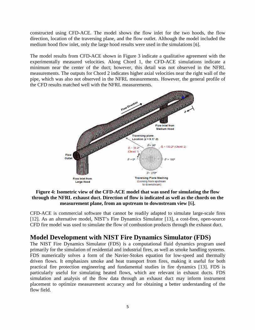
constructed using CFD-ACE. The model shows the flow inlet for the two hoods, the flow direction, location of the traversing plane, and the flow outlet. Although the model included the medium hood flow inlet, only the large hood results were used in the simulations [6]. The model results from CFD-ACE shown in Figure 3 indicate a qualitative agreement with the experimentally measured velocities. Along Chord 1, the CFD-ACE simulations indicate a minimum near the center of the duct; however, this detail was not observed in the NFRL measurements. The outputs for Chord 2 indicates higher axial velocities near the right wall of the pipe, which was also not observed in the NFRL measurements. However, the general profile of the CFD results matched well with the NFRL measurements.

Figure 4: Isometric view of the CFD-ACE model that was used for simulating the flow

through the NFRL exhaust duct. Direction of flow is indicated as well as the chords on the measurement plane, from an upstream to downstream view [6].

CFD-ACE is commercial software that cannot be readily adapted to simulate large-scale fires [12]. As an alternative model, NIST’s Fire Dynamics Simulator [13], a cost-free, open-source CFD fire model was used to simulate the flow of combustion products through the exhaust duct. Model Development with NIST Fire Dynamics Simulator (FDS) The NIST Fire Dynamics Simulator (FDS) is a computational fluid dynamics program used primarily for the simulation of residential and industrial fires, as well as smoke handling systems. FDS numerically solves a form of the Navier-Stokes equation for low-speed and thermally driven flows. It emphasizes smoke and heat transport from fires, making it useful for both practical fire protection engineering and fundamental studies in fire dynamics [13]. FDS is particularly useful for simulating heated flows, which are relevant in exhaust ducts. FDS simulation and analysis of the flow data through an exhaust duct may inform instrument placement to optimize measurement accuracy and for obtaining a better understanding of the flow field.

6

FDS lacks the ability to create geometries in a polar coordinate system. This makes the program less useful for simulating the flow through the circular geometries of an exhaust duct. In the following sections, the process of developing a series of FDS models for simulating the flow through a cylindrical NFRL exhaust duct is described. The process evolved from a simple, rectangular model of the duct, to more detailed and physically accurate models. For each model, reduced scale domains were tested to fully understand model results and check accuracy.

Square Duct Model The simplest construction of an exhaust duct with FDS is by using a square cross section. FDS simulates square geometry easily making it useful to quickly test the model and visualize the flow physics. Figure 5 displays a square duct model with bends to simulate the flow through an exhaust duct. The 180o horizontal bend was approximated by two 90o bends (square bends) and was produced with three speared meshes. A no-slip condition was applied at the walls and gas temperature at the inlet was set at 297 K [6]. These conditions were used for all FDS simulations described in this report. U-Velocity (velocity in the streamwise direction) is displayed in multiple slices as a color contour. Note that the flow appears to be uniform in section 1, but is turbulent as it traverses through section 3. Incorporating the bend in the model is necessary to model the flow asymmetry that is observed in the experimental data. However, since the 180o horizontal bend was modeled with square bends, it resulted in vortices and higher levels of turbulence in section 3.

Figure 5: Isometric view of the square duct model with bends to represent the exhaust duct.

The inlet section is labeled as 1, the 180o bend is labeled 2 and the outlet is labeled as 3.

Circular Pipe Model The square duct model displayed asymmetry in the axial velocity profile observed in section 3 consistent with experimental measurements (see Figure 3), but lacked the correct circular geometry of the NFRL exhaust duct. This section describes the process of altering the cross section of the exhaust duct model from square to circular geometry as well as the method used to incorporate the 180o horizontal bend and the 90o vertical bend (seen in Figure 1, Figure 3). A “Stacked Cylinders” approach was utilized, where cylinders of increasing length and decreasing

3

2

1

7

radius were formed around the same center point. By stacking these cylinders on top of each other, there was a stair-step effect that mimicked the curvature of the bend (as shown in Figure 6). There was no mathematical basis for this method, instead a qualitative and iterative approach was used to simulate the curvature. Figure 6 is a schematic of the stack cylinder method to generate bends and to approximate the exhaust duct geometry.

Figure 6: Application of the stacked cylinders approach to create a 180 o bend.

Figure 7 shows the full exhaust duct model incorporating the horizontal 180o bend (section 2) as well as the large hood inlet (section 6). The stacked cylinder method was also used to decrease the duct diameter, when flow from section 4 transitions into section 1. Axial velocity slices are shown along the entire duct indicating that the flow transitions into a turbulent flow after section 2. The inlet was located at the bottom of the vertical section of duct (section 5, Figure 7).

Figure 7: Isometric view of the full circular pipe model with horizontal and vertical bends. U-

Velocity slices at T = 92.0 s displayed throughout the model.

Toroidal Model Development The stacked cylinders method (described in the previous section) featured “rounded” corners at the vertical and horizontal bends of the exhaust duct (section 6 and section 2 in Figure 7 respectively). Blueprints of the NFRL exhaust duct and photographs (Figure 1) indicate that the

4

5

6

3

2

1

8

vertical and horizontal bends were toroidal in shape. They were not straight sections with rounded corners. Accordingly, the geometry of the bends in the exhaust duct was modified to that of hollow torus instead of the stair-step cylinders to accurately capture the flowfield. The torus itself was a hollow shell connected to the straight sections of the duct. Construction of an appropriate model of the exhaust duct required the use of half a torus for the 180o horizontal bend (section 2), and a quarter torus for the 90o vertical bend (section 6). Each torus was made of individual obstruction cubes with a side length equal to the grid spacing. By evaluating each individual mesh cell in the relevant domain and checking whether or not the torus would pass through it, a detailed torus was generated. Figure 8 displays a simple torus in three dimensional space, with a grid over the surface of the torus. The radius of the pink circle is referred to as the major radius “R” of the torus, while the radius of the red circle is referred to as the minor radius “r”. The equation for a torus [14] in the x-y plane can be written as

[(x – xi)2+(y – yi)2+(z – zi)2 + R2 - r2]2 - 4*(R2)*[(x – xi)2+(y – yi)2] = 0, (1)

where, (xi, yi, zi) are the co-ordinates of the center of the torus in Cartesian space. The major radius (R) and minor radius (r) were set to 1.8 m and 0.8 m, respectively, for the 180o horizontal bend (section 2). For the 90o vertical bend (section 6), the major and minor radiuses were set to 1.2 m and 1.1 m, respectively. Each cell of the domain was evaluated to determine if its center (x, y, z) was inside the equation defined by the torus. Obstructions in the FDS input file were created depending on this evaluation.

Figure 8: The surface of a torus. The radius of the pink and red circles are defined as the

major (R) and minor (r) radiuses, respectively.

The approach described in the previous section was applied in two areas: the 180o horizontal bend at section 2 and then the 90o vertical bend at section 6. The left sub-figure of Figure 9 is a top view of the torus geometry developed for the180o horizontal bend (section 2). The bend extends from the straight cylindrical sections at section 1 and reconnects at section 3. The right sub-figure of Figure 9 is a side view of the 90o vertical bend (section 6), with the x-z grid shown

9

for scale. The bend extends from the inlet at section 5 and reconnects at section 4. The grid spacing for both of these bends was 5.0 cm. The outlet is highlighted with a pink outline in the left sub-figure of Figure 10, and shows the approximation of the circular exhaust duct geometry. The right sub-figure of Figure 10 displays a full isometric view of the model. Included are the 180o horizontal bend and 90o vertical bend, as well as the large hood inlet.

Figure 9: Left: Top view of the final horizontal toroidal bend constructed using a5.0 cm

grid spacing. Right: Isometric view of the vertical toroidal bend.

Figure 10: Left: Front view of the duct outlet of the exhaust duct using 5.0 cm grid spacing.

Right: Isometric view of the final FDS model of the exhaust duct.

Convergence Studies Simulations were conducted at increasing mesh resolutions to test for the dependence of results on grid cell size. The final model shown in Figure 10 (right sub-figure) was used for these convergence studies. This final model included the toroidal bends at sections 2 and 6. Grid cell size was varied uniformly with cubic grid cell dimensions of 10.0 cm, 6.25 cm, 5.0 cm, and 3.33 cm in the separate test. The inlet mass flux was set at 7.65 kg/m2/s based on the 23.0 kg/s mass flow rate. In addition to mesh resolution, the effect of smoothing the flow near surfaces was also considered. Smoothing is achieved in FDS by ignoring the vorticity term in the momentum

5

6

4

2

3

1

3

2 1

4

6

5

3

10

equation, effectively stopping the vortices generated by the edges of solid objects, such as those comprising the curved duct walls. Table 1 displays the computed mass flow rate (kg/s) for the five different grid cell sizes as well as for the smoothed and unsmoothed boundaries. Results indicate that regardless of grid spacing or the smoothing option, the computed mass flow rates are consistently near the target value of 23.0 kg/s.

Table 1: FDS results mass flow (in kg/s) for various uniform grid spacing and Sawtooth options.

Grid Spacing in cm Mass flow (kg/s) 10.0 cm 6.25 cm 5.0 cm 3.85 cm 3.33 cm Sawtooth option = .TRUE. 22.36 23.13 23.21 22.69 22.76 Sawtooth option = .FALSE. 22.62 23.72 24.04 23.38 23.64

However, the axial velocity profile obtained from the Sawtooth= .FALSE. option (smoothed boundary) in FDS produced non-physical results as it does not maintain the no-slip condition at the walls of the duct. FDS results for the axial velocity profile are shown in Figure 11 (Sawtooth = .FALSE. option). Near the walls of the duct at radii of -0.75 m and 0.75 m, the velocity should approach zero. However, this is not the case for Chord 1 or Chord 2, as shown in Figure 11. The Sawtooth=.TRUE. (default) value was used for all the calculations discussed in this report.

Figure 11: FDS simulation results using the Sawtooth = .FALSE. option. Axial velocity is plotted as a function of radius for Chord 1 (left sub-figure) and Chord 2 (right sub-figure).

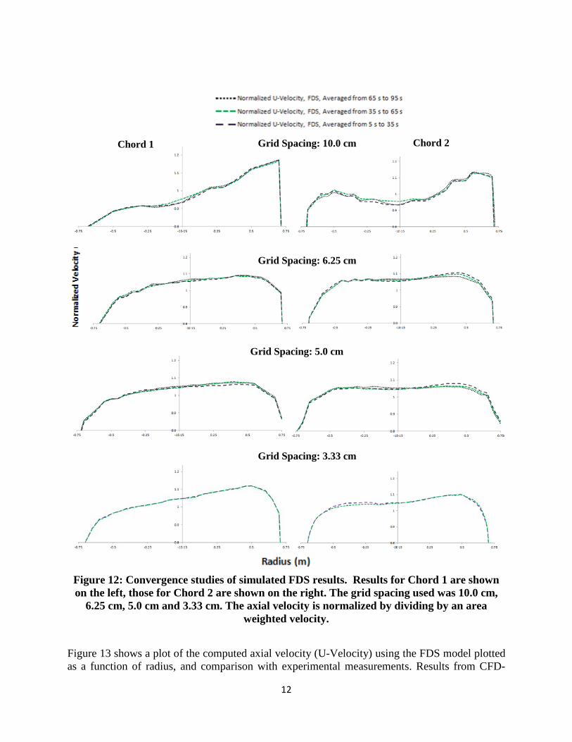
Figure 12 shows a series of graphs of axial velocity as a function of radius for different grid spacing. Plots in the left and right columns represent normalized velocity profiles at Chord 1 and Chord 2, respectively. Results for grid cell values of 10.0 cm, 6.25 cm, 5.0 cm, and 3.33 cm are shown. The axial velocity (normalized) was computed at the plane X = - 2.0 m in section 3, averaged over three 30 s time frames. The FDS results were normalized by dividing the computed U-Velocity by the area weighted velocity: 10.72 m/s for 10.0 cm spacing, 11.09 m/s for the 6.25 cm spacing, and 11.13 m/s for the 5.0 cm spacing. Results shown in Figure 12 indicate that the profiles do not change significantly below grid cell sizes of 6.25 cm, indicating a

Chord 2 Chord 1 Grid Spacing: 10.0 cm

11

convergence of results. Accordingly, grid cell dimensions of 5.0 cm were used in the simulations described below. Comparison of FDS Simulation Results and Experimental Data In this section, we compare FDS simulation results with experimental data that were presented in the previous section. The choice of FDS model and grid resolution has been discussed in the previous sections. In order to compare the simulation results with experimental data, the mass flow rate from two specific experiments, one for each chord, was used. A mass flow rate of 21.3 kg/s was used for velocity measurements at Chord 1 position, while a mass flow rate of 20.2 kg/s was used for Chord 2. The mass flux used for the numerical simulations was set at 7.1 kg/m2/s for the Chord 1 case and 6.7 kg/m2/s for the Chord 2 case.

12

Figure 12: Convergence studies of simulated FDS results. Results for Chord 1 are shown on the left, those for Chord 2 are shown on the right. The grid spacing used was 10.0 cm,

6.25 cm, 5.0 cm and 3.33 cm. The axial velocity is normalized by dividing by an area weighted velocity.

Figure 13 shows a plot of the computed axial velocity (U-Velocity) using the FDS model plotted as a function of radius, and comparison with experimental measurements. Results from CFD-

Chord 2 Chord 1 Grid Spacing: 10.0 cm

Grid Spacing: 6.25 cm

Grid Spacing: 5.0 cm

Grid Spacing: 3.33 cm

13

ACE software have also been included for comparison with FDS simulations. Note that the axial velocity (m/s) has not been normalized with the annubar velocity. The top sub-figure shows results for Chord 1, while the bottom sub-figure shows similar data for Chord 2. Results indicate that FDS simulations predict a lower axial velocity for Chord 1 on the left side of the duct (R = -0.75m) and higher axial velocity on the right side (R = 0.75 m), as compared with experimental data. FDS results for Chord 2 are higher than the experimental data on the left side of the duct and lower on the right side. The variations that exist between the simulated results and experimental data could be due to several parameters such as the roughness of the duct, inlet flow turbulence, or any gradient of the exhaust duct that have not been included in the FDS model.

Figure 13: Comparison of FDS simulation results, CFD-ACE data and experimental measurements for axial velocity plotted as a function of duct radius. Results are shown for

Chord 1 (top sub-figure) and Chord 2 (bottom sub-figure).

FDS

Chord 1 Grid Spacing: 5.0 cm

Chord 2

Axial Velocity, CFD-ACE

FDS

CFD-ACE

CFD-ACE

14

The basic flow physics that is simulated with FDS is the fluid flow around the bends (horizontal bend at section 6, and the vertical bend at section 2). As the flow moves through a bend, centrifugal effects would accelerate the flow at the outer edge of the bend, while a velocity deficit would be obtained at the inner edge of the bend (mass balance). Due to the 90o bend (section 6), higher velocity should be obtained in the upper half of the duct after the vertical bend. Similarly, after the 180o bend (section 2), higher velocity should be observed in the outer half of the duct. These higher velocities are also due to the centrifugal effects of flow turning around a bend. Figure 14 displays the flowfield (axial velocity) through the bends in the exhaust duct. The left sub-figure displays the flow field through the vertical bend (section 6) and the right sub-figure displays the flow field through the horizontal bend (section 2). The FDS results are clearly consistent with the flow physics presented above as shown in the sub-figures for Figure 14 as well as the experimental data from the NFRL experiments.

Figure 14. Visualization of the flow field through the vertical bend (section 6) is shown in

the left sub-figure, while that through horizontal bend (section 2) is shown in the right sub-figure.

Discussion and Conclusions The NIST National Fire Research Laboratory has conducted greenhouse gas emission measurement tests through detailed measurements within an exhaust duct. The experiments were simulated with the NIST Fire Dynamics Simulator (FDS) to obtain a detailed understanding of the flow field through an exhaust duct and for providing guidance for future experiments. Since FDS lacks the ability to create geometries in a polar coordinate system, it cannot be used directly to model the flow through the cylindrical geometry of an exhaust duct. The bends in the exhaust duct make it especially difficult to model the flow field using FDS. In this report, we describe the stacked cylinder approach and a methodology that is based on the equation of a torus to carve a cylindrical geometry in a block that is divided into rectilinear grids. A model of the NFRL exhaust duct was created using this approach. Grid convergence studies were completed to ensure that the computed results were independent of grid resolution. Parametric studies were performed to understand the effect of varying mass flow rate through the exhaust duct. The FDS simulation results compared favorably with measured NFRL

15

experimental data in the center of the exhaust duct, however, differences were observed towards the outer portions of the duct. Differences in the simulated and measured profiles may be due to roughness of the exhaust duct, inlet turbulence and tilt of the duct. Incorporating these effects into the model could improve the comparison between experimental data and simulations. References

1. Hofman, D. J., J. H. Butler, E. J. Dlugokencky, J. W. Elkins, K. Masarie, S. A. Montzka, and P. Tans (2006), The role of carbon dioxide in climate forcing from 1979-2004: Introduction of the Annual Greenhouse Gas Index, Tell us B, 58B, 614-619.

2. Keeling, C. D., R.B. Bacastow, A. F. Carter, S.C. Piper, T.P. Wharf, M. Heimann, W.G. Mook, and H. Roeloffzen 1989. A three-dimensional model of atmospheric C02 transport based on observed winds: 1. Analysis of observational data. In D.H. Peterson (ed.), Aspects of Climate Variability in the Pacific and the Western Americas. Geophysical Monograph 55:165-235.

3. NRC Report, Pacala, S.W., Breidenich, C., Brewer, P.G., Fung, I.Y., Gunson, M.R., and coauthors: Verifying greenhouse gas emissions: Methods to support international climate agreements, 2010. Committee on methods for estimating greenhouse gas emissions, National Research Council, The National Academies Press, 500 Fifth Street, N.W., Washington, D.C., 20001. Available at http://www.nap.edu.

4. Nisbet, E., and R. Weiss, 2010. Top-down versus bottom-up. Science, 328, 1241-3.

5. Prinn, R. G., Heimbach, P, Rigby, M., Dutkiewicz, S., Melillo, J. M., Reilly, J. M., Kicklighter, D. W., Waugh, C. J., A Strategy for Global Observing System for Verification of National Greenhouse Gas Emissions, Report No. 200, June 2011.

6. IPCC, 2007, Climate Change 2007, The Physical Science Basis, Working Group I

Contribution to the Fourth, Assessment Report of the Intergovernmental Panel on Climate Change, Cambridge University Press.

7. Bryant, R.A.; Sanni, O.; Moore, E.; Borthwick, R. P.; Fernandez, M.; Shinder, I.;Yang, J.; Johnson, A. Comparison of Gas Velocity Measurements and CFD Predictions in the Exhaust Duct of a Stationary Source, EPRI CEM User Group Conference, 2011.

8. Bryant, R. A.; Ohlemiller, T. J.; Johnsson, E. L.; Hamins, A.; Grove, B. S.; Guthrie, W. F.; Maranghides, A.; Mulholland, G. W. The NIST 3 Megawatt Quantitative Heat Release Rate Facility; NIST Special Publication 1007; National Institute of Standards and Technology: Gaithersburg, MD, 2003.

9. Sample and Velocity Traverses for Stationary Sources - EPA Method 1, Environmental

Protection Agency Report, 2000. http://www.epa.gov/ttn/emc/promgate/m-01.pdf

16

10. Determination of Stack Gas Velocity and Volumetric Flow Rate (Type S Pitot Tube) – EPA Method 2, Environmental Protection Agency Report, 2000. http://www.epa.gov/ttn/emc/promgate/m-02.pdf

11. Determination of Stack Gas Velocity and Volumetric Flow Rate With Two-Dimensional Probes - EPAMethod 2G, Environmental Protection Agency Report 2007. http://www.epa.gov/ttn/emc/promgate/Methd2G.pdf

12. ESI Group “CFD-ACE” http://www.esi-group.com/products/multiphysics/ace-multiphysics-suite/ace-suite/cfd-ace

13. McGrattan, K.B., Baum, H. R., Rehm, R., Hamins, A., Forney, G. P., Floyd, J. E., Hostikka, S., Prasad, K., Fire Dynamics Simulator User’s Guide, NISTIR 6784, 2002, Ed. 2002.

14. Wikipedia, The Free Encyclopedia, http://en.wikipedia.org/wiki/Torus