Air Dispersion Modeling Guidelines for Arizona Air Quality Permits

PREPARED BY:

AIR QUALITY PERMIT SECTION

AIR QUALITY DIVISION

ARIZONA DEPARTMENT OF ENVIRONMENTAL QUALITY

December 1, 2015

TABLE OF CONTENTS

1 INTRODUCTION.......................................................................................................... 1 1.1 Overview of Regulatory Modeling ........................................................................... 2 1.2 Purpose of an Air Quality Modeling Analysis .......................................................... 2 1.3 Authority for Modeling ............................................................................................. 3 1.4 Acceptable Models.................................................................................................... 3 1.5 Overview of Modeling Protocols and Checklists ..................................................... 4 1.6 Overview of Modeling Reports ................................................................................ 5

2 LEVELS OF MODELING ANALYSIS SOPHISTICATION .................................. 5 2.1 Screening Modeling .................................................................................................. 6 2.2 Refined Modeling ..................................................................................................... 7

3 MODELING ANALYSIS FEATURES ..................................................................... 10 3.1 Modeling Worst-Case Scenarios............................................................................. 10

3.1.1 Emissions Profiles ............................................................................................ 10 3.1.2 Load Analyses .................................................................................................. 11 3.1.3 Emission Caps .................................................................................................. 12

3.2 Modeling Emissions Inventory ............................................................................... 12 3.3 Types of Sources ..................................................................................................... 13

3.3.1 Point Sources ................................................................................................... 13 3.3.2 Volume Sources ............................................................................................... 14 3.3.3 Area Sources .................................................................................................... 15 3.3.4 Line Sources ..................................................................................................... 16 3.3.5 Road Emission Sources .................................................................................... 16 3.3.6 Flares ................................................................................................................ 17 3.3.7 Open Pit Sources .............................................................................................. 19 3.3.8 Pseudo Point / Non-Standard Point Source ..................................................... 19 3.3.9 Emission Point Collocation .............................................................................. 20

3.4 Ambient Air Boundary ........................................................................................... 20 3.4.1 Definition of General Public ............................................................................ 21 3.4.2 Public Access ................................................................................................... 21 3.4.3 Property without an Effective Fence or Other Physical Barriers ..................... 22 3.4.4 Leased Property ............................................................................................... 22

3.5 Modeling Coordinate Systems ................................................................................ 22 3.6 Receptor Networks.................................................................................................. 23 3.7 Rural/Urban Classification ...................................................................................... 24 3.8 Meteorological Data................................................................................................ 27

3.8.1 Meteorological Data Description and Rationale .............................................. 29 3.8.2 Meteorological Data Processing ...................................................................... 30

3.9 Building Downwash and GEP Stack Height .......................................................... 31 3.10 Background Concentrations .................................................................................. 32 3.11 Modeled Design Concentrations ........................................................................... 35

4 ADEQ PERMITTING JURISDICTION AND CLASSIFICATIONS ................... 37 4.1 Air Quality Permitting Jurisdiction in Arizona ....................................................... 37 4.2 Modeling Requirements for Permits and Registration............................................ 38

4.2.1 Classes of Permits and Registration ................................................................. 38

i

4.2.2 Modeling Requirements ................................................................................... 38 5 MODELING REQUIREMENTS UNDER MINOR NSR AND REGISTRATION PROGRAM ..................................................................................................................... 43

5.1 Modeling Demonstration for Attainment Pollutants............................................... 43 5.2. Modeling Demonstration for Nonattainment Pollutants ........................................ 44

6 MODELING REQUIREMENTS FOR PSD SOURCES ......................................... 45 6.1 NAAQS Analyses for Pollutants That Do Not Trigger PSD .................................. 46 6.2 Overview of PSD Modeling Procedures ................................................................. 46

6.2.1 NAAQS Modeling Inventory ........................................................................... 48 6.2.2 Increment Modeling Inventory ........................................................................ 49 6.2.3 Additional Impact Analyses ............................................................................. 51 6.2.4 Class I Area Impact Analyses .......................................................................... 52

7 SPECIAL MODELING ISSUES ................................................................................ 54 7.1 Modeling for 1-hour NO2........................................................................................ 54

7.1.1 Emission Rate .................................................................................................. 55 7.1.2 Significant Impact Level .................................................................................. 55 7.1.3 Three-tiered Approach for 1-hour NO2 Modeling ........................................... 56 7.1.4 Determining Background Concentrations ........................................................ 56 7.1.5 In-Stack NO2/NOX Ratio .................................................................................. 59 7.1.6 Treatment of Intermittent Sources ................................................................... 59 7.1.7 Modeling Demonstration with the 1-hour NO2 NAAQS ................................. 60

7.2 Modeling for 1-hour SO2 ........................................................................................ 62 7.2.1 Emission Rate .................................................................................................. 62 7.2.2 Significant Impact Level .................................................................................. 63 7.2.3 Determining Background Concentrations ........................................................ 63 7.2.4 Treatment of Intermittent Sources ................................................................... 64 7.2.5 Modeling Demonstration with the 1-hour SO2 NAAQS ................................. 64

7.3 Modeling for PM2.5 ................................................................................................. 65 7.3.1 Significant Monitoring Concentration and Significant Impact Levels ............ 66 7.3.2 Modeling Primary PM2.5 and Secondarily Formed PM2.5 ................................ 67 7.3.3 Emission Inventories ........................................................................................ 69 7.3.4 Background Concentration .............................................................................. 70 7.3.5 Comparison to the SIL ..................................................................................... 71 7.3.6 Modeling Demonstration with the PM2.5 NAAQS .......................................... 71 7.3.7 Modeling demonstration with the PM2.5 Increments ....................................... 72 7.3.8 Modeling PM2.5 under the Minor NSR Program AND Registration Program . 73

7.4 Additional Considerations for Modeling Particulate Matter (PM) ......................... 75 7.4.1 Paired-Sums Approach .................................................................................... 75 7.4.2 Particle Deposition ........................................................................................... 75

7.5 Modeling for Lead (Pb) .......................................................................................... 76 7.6 Modeling for Open Burning/Open Detonation Sources ......................................... 76

7.6.1 Modeling OB/OD Operations with OBODM .................................................. 76 7.6.2 Modeling OB/OD Operations with AERMOD ................................................ 77

7.7 Modeling for Buoyant Line Sources ....................................................................... 77 7.8 Modeling for HAPS Sources - Learning Site Policy .............................................. 78

8 REFERENCES .......................................................................................................... 78

ii

APPENDIX A: MODELING PROTOCOL ELEMENTS .......................................... 83 APPENDIX B: LEARNING SITES POLICY IMPLEMENTATION PLAN ........ 87 APPENDIX C: ACUTE AND CHRONIC AMBIENT AIR CONCENTRATIONS 89

LIST OF TABLES Table 1 AERSCREEN Scaling Factors .............................................................................. 7 Table 2 Suggested Procedures for Estimating Volume Source Parameters ..................... 14 Table 3 Suggested Receptor Spacing ................................................................................ 23 Table 4 Auer Land -Use Classifications ........................................................................... 27 Table 5 Calculation of GEP Stack Height ........................................................................ 32 Table 6 Determination of Background Concentrations .................................................... 34 Table 7 Modeled Design Concentrations .......................................................................... 36 Table 8 Permitting Exemption Thresholds ....................................................................... 39 Table 9 PSD Increments, Significant Emission Rates, Modeling Significance Levels, and Monitoring De Minimis Concentrations ........................................................................... 47 Table 10 Major Source Baseline Dates ............................................................................. 50 Table 11Minor Source Baseline Dates for Arizona AQCRs ............................................ 50 Table 12 Class I Areas Located in Arizona ...................................................................... 53 Table 13 Calculated 98th Percentile Value Based on the Annual Creditable Number of Samples ............................................................................................................................. 70

LIST OF FIGURES

Figure 1 Locations of ADEQ AERMET Meteorological Data Sets ................................. 28 Figure 2 Map of Arizona................................................................................................... 41 Figure 3 Tribal Lands in Arizona...................................................................................... 42 Figure 4 Air Quality Control Regions in Arizona ............................................................ 51 Figure 5 Class I Areas in Arizona ..................................................................................... 54

iii

ACRONYMS AND ABBREVIATIONS AAAC Acute Ambient Air Concentrations AAB Ambient Air Boundary AAC Arizona Administrative Code ADEQ Arizona Department of Environmental Quality AERMAP Terrain data preprocessor for AERMOD AERMET Meteorological data preprocessor for AERMOD AERMIC American Meteorological Society/Environmental Protection Agency Regulatory Model Improvement Committee AERMOD AMS/EPA Regulatory Model AERSCREEN Screening version of AERMOD AERSURFACE Surface characteristics preprocessor for AERMOD AIWG AERMOD Implementation Workgroup AMS American Meteorological Society AQCR Air Quality Control Region AQRV Air Quality Related Value ARM Ambient Ratio Method ASOS Automated Surface Observing Systems BPIP Building Profile Input Program CAA Clean Air Act CAAC Chronic Ambient Air Concentrations CALMET Meteorological data preprocessor for CALPUFF CALPOST Postprocessor for CALPUFF CALPUFF California Puff Model CASTNET Clean Air Status and Trends Network DEM Digital Elevation Model EPA Environmental Protection Agency FLAG Federal Land Managers’ Air Quality Related Values Work Group FLM Federal Land Manager GAQM Guideline on Air Quality Models GEP Good Engineering Practice HAP Hazardous Air Pollutants IMPROVE Interagency Monitoring of Protected Visual Environments ISCST3 Industrial Source Complex, Short Term Ver. 3 IWAQM Interagency Workgroup on Air Quality Modeling MACT Maximum Achievable Control Technology MERP Model Emissions Rates for Precursors MM5 Penn State/NCAR Fifth Generation Mesoscale Model

iv

MMIF Mesoscale Model Interface Program MRLC Multi-Resolution Land Characteristics NAA Nonattainment Area NAAQS National Ambient Air Quality Standards NACAA National Association of Clean Air Agencies NCDC National Climatic Data Center NED National Elevation Dataset NNSR Non-attainment Area New Source Review NSR New Source Review NWS National Weather Service OAQPS Office of Air Quality Planning and Standards OBODM Open Burn/Open Detonation Model OLM Ozone Limiting Method PRIME Plume Rise Model Enhancements PSD Prevention of Significant Deterioration PTE Potential To Emit PVMRM Plume Volume Molar Ratio Method SCRAM EPA Support Center for Regulatory Air Models SER Significant Emission Rate SIA Significant Impact Area SIL Significant Impact Level SIP State Implementation Plan SMC Significant Monitoring Concentration SoDAR Sonic Detection And Ranging USGS U.S. Geological Survey UTM Universal Transverse Mercator WRF Weather Research and Forecasting

v

1 INTRODUCTION This guidance document has been developed by the Air Quality Division (AQD) of the Arizona Department of Environmental Quality (ADEQ) to document air quality modeling procedures for air quality permit applications for sources located in Arizona under ADEQ jurisdiction. This guidance provides assistance to the Permittee required to perform modeling analyses to demonstrate that the air quality impacts from new and existing sources protect public health, general welfare, physical property, and the natural environment. This guideline is not intended to supersede statutory or regulatory requirements or more recent guidance of the state of Arizona or the U.S. Environmental Protection Agency (EPA). It is assumed that the reader of these guidelines has a basic knowledge of modeling theory and techniques. At a minimum, individuals responsible for conducting an air quality modeling analysis should be familiar with the following documents:

• Guideline on Air Quality Models (GAQM) as codified in 40 CFR 51, Appendix W (U.S. EPA, 2005);

• Draft New Source Review Workshop Manual (U.S. EPA, 1990); • Screening Procedures for Estimating the Air Quality Impact of Stationary Sources

(U.S. EPA, 1992a); • Guidance and clarification memoranda issued by the EPA Office of Air Quality

Planning and Standards (OAQPS); • Guidance issued by EPA Region 9; and • User’s guides for each dispersion model.

This publication replaces the previous edition of ADEQ’s Modeling Guidelines (ADEQ, 2004). This guidance clarifies issues described in EPA documents, facilitates development of an acceptable modeling analysis, and assists ADEQ in expediting the permit review process. The guidelines also outline additional modeling requirements specific to ADEQ. While ADEQ has attempted to address as many issues as possible, each modeling analysis is still treated on a case-by-case basis. Therefore, the Permittee should work closely with ADEQ staff to ensure that all modeling requirements are met. If the Permittee can demonstrate that techniques other than those recommended in this document are more appropriate, then AQD may approve their use. ADEQ reserves the right to make adjustments to the modeling requirements of each permit application on a case-by-case basis. This document will be amended periodically to incorporate new modeling guidance and changes to regulations.

1

1.1 Overview of Regulatory Modeling Air quality modeling is utilized to predict ambient impacts of one or more sources of air pollution. Equations and algorithms representing atmospheric processes are incorporated into various dispersion models. The equations and algorithms used in the models are based on both known atmospheric processes and empirical data. ADEQ uses the results of modeling analyses to determine if a new or existing source of air pollutants complies with state and federal maximum ambient concentration standards and guidelines. Air quality models are useful in properly designing and configuring sources of pollution to minimize ambient impacts. The most commonly used air quality models for regulatory applications generally fall into two categories: dispersion models and photochemical grid models. Dispersion models are typically used in the permitting process to estimate the concentration of pollutants at specified ground-level receptors surrounding an emissions source. Photochemical grid models are typically used in regulatory or policy assessments to simulate the impacts from all sources by estimating pollutant concentrations and deposition of both inert and chemically reactive pollutants over large spatial scales. This guidance document addresses dispersion modeling as a regulatory tool. Owing to the intrinsic uncertainty of air quality modeling, a modeled prediction alone does not necessarily indicate a real-world pollution condition. However, a modeled prediction of an exceedance of a standard or guideline may indicate the possibility of potential real-world air quality violations. The impacts of new sources that have not been constructed can only be determined through air quality modeling. Moreover, monitoring data normally are not sufficient as the sole basis for demonstrating the adequacy of emission limits for existing sources because of the limitations in the spatial and temporal coverage. Therefore, air quality models have become a critical analytical tool in air quality assessments. In particular, they are widely used as a basis to modify allowable emission rates, stack parameters, operating conditions, or to require state implementation plan review for criteria pollutants.

1.2 Purpose of an Air Quality Modeling Analysis An air quality modeling analysis is used to determine that criteria pollutants or hazardous air pollutants emitted from a source will not cause or significantly contribute to a violation of any National Ambient Air Quality Standard (NAAQS), or Prevention of Significant Deterioration (PSD) increment, or Arizona Acute/Chronic Ambient Air Concentrations (AAAC and CAAC) for listed hazardous air pollutants (HAPs). An overview of modeling analyses required by ADEQ for minor sources is described in Section 5. An overview of PSD modeling analyses is provided in Section 6. An overview of HAPs modeling analyses is provided in Section 7.8. Air quality modeling analyses may also be required to:

2

• Determine whether air quality monitoring is required and appropriately locate air quality and/or meteorological monitors,

• Determine the impacts on Class I and Class II Areas as a result of emissions from new or modified sources,

• Determine if, for a PSD source located within 10 kilometers of a federal Class I Area, the source’s net emissions increase has an impact of 1 μg/m3 (24-hour average) or more,

• Determine if, for any pollutant, a concentration will exist that may pose a threat to public health or welfare or unreasonably interfere with the enjoyment of life or property (e.g. odor), and/or

• Perform a human health or ecological risk assessment.

1.3 Authority for Modeling Arizona Revised Statutes (A.R.S.) §49-422, describes the powers of the ADEQ Director related to the quantification of air contaminants. Arizona Administrative Code (A.A.C.) R18-2-407 requires air dispersion modeling for new major sources and major modifications to existing sources. The State of Arizona Minor NSR program (R18-2-334 of the A.A.C.) will be effective on December 2, 2015. The minor NSR program provides an opportunity to the Permittee to address minor NSR changes by conducting a NAAQS modeling exercise or to conduct a Reasonable Available Control Technology (RACT) analysis. Notwithstanding the Permittee’s election to conduct a RACT analysis, the Director may request the Permittee conduct a NAAQS analysis if a source or a minor NSR modification could interfere with attainment and maintenance of the NAAQS.. The State of Arizona registration program (R18-2-302.01 of the A.A.C.) will be effective on December 2, 2015. Based on the Director’s discretion, ADEQ may perform modeling for criteria pollutants of concern on a case-by-case basis. ADEQ’s modeling exercise will be limited to a screening analysis.

1.4 Acceptable Models In general, ADEQ adheres to EPA’s Guideline on Air Quality Models (GAQM) codified in 40 CFR 51, Appendix W, to determine acceptable models for use in air quality impact analyses (U.S. EPA, 2005). This document provides guidance on appropriate modeling applications. As new models are accepted by EPA, the Guideline on Air Quality Models is updated. A “preferred model” as specified in the GAQM is acceptable for the type of regulatory modeling for which it is designed. For example, the preferred near-field (less than 50 kilometers from the source) dispersion model for industrial sources is the American Meteorological Society (AMS)/EPA Regulatory Model (AERMOD) and the preferred

3

long-range transport (beyond 50 kilometers from the source) dispersion model is California Puff Model (CALPUFF). First tier models also include BLP and Cal3QHC. A second tier of models are the “alternative models” as specified in GAQM. These models could be used in situations where ADEQ has found them to be more appropriate than a preferred model. However, the Permittee must seek ADEQ approval to use any alternative model. ADEQ reserves the right to evaluate the use of alternative models on a case-by-case basis. Additionally, depending on the situation, the model evaluation may require the approval by EPA Region 9 and/or be subject to public review. More information regarding dispersion modeling, including models available for download, is available at EPA’s Support Center for Regulatory Air Models (SCRAM) website at http://www.epa.gov/ttn/scram.

1.5 Overview of Modeling Protocols and Checklists Modeling protocols and guidance checklists outline how modeling analyses should be conducted and how a modeling analysis will be presented. It is through such documents that ADEQ is attempting to expedite the permitting process. In a modeling protocol, emission sources should be discussed in sufficient detail, and include the derivation of all source parameters. Those parameters should be derived from the final source configuration, or if not finalized, approximated from the best available information at the time the protocol is developed. Protocols should also address the relevant modeling requirements and recommendations from state/federal regulations and air quality modeling guidelines. ADEQ recognizes that many air quality specialists have their own preferred formats for protocols. ADEQ does not wish to require Permittees to use a specific modeling protocol format. Instead, ADEQ has generated a listing of typical protocol elements as an aid in developing a modeling protocol. This listing does not address all possible components of a protocol. Case-by-case judgments should be used to decide if additional aspects of an analysis should be included in the protocol or if certain elements are not necessary in a given situation. An example list of modeling protocol elements is provided in Appendix A. It is highly recommended that Permittees submit a modeling protocol to ADEQ for approval prior to commencing a refined modeling or PSD modeling analysis. A modeling report without a pre-approved modeling protocol will be treated and reviewed as a protocol. Permittees are encouraged to submit a modeling protocol electronically (email is acceptable). Complete hard copies of the protocol will be accepted but must be accompanied with a CD, DVD or other means containing an electronic copy of the submission. In general, the protocol submittal should be sent to the ADEQ’s Permits Section where a permit review staff processes the permit application. However, it is appropriate for Permittees or their modelers to send modeling protocols directly to modeling staff in the ADEQ’s Permits Section. If doing so, a copy must also be sent to the permit review staff since he/she is responsible for the overall review of the permit. Depending on the project, Permittees may need to send a protocol copy to federal

4

agencies such as EPA Region 9 and the affected federal land managers. ADEQ will make the determination as to which federal agencies and other entities should also be sent a copy of the protocol, but Permittees are free to distribute the protocol more widely. Permittees should allow a minimum of two (2) weeks for ADEQ to review a modeling protocol. Upon completion of the review, Permittees will receive either a written or email notification of acceptance of the modeling approach, or a written or email request for additional information which may contain guidance on any issues needing further clarification. ADEQ will issue a written or email approval of a modeling protocol once agreement is reached. Permittees should understand that an approved modeling protocol does not necessarily limit the extent of the modeling that will be required. Additional modeling may be required as determined by ADEQ on a case-by-case basis. In some cases checklists may be required for review but are for the purpose of Permittee guidance and expediting the review, and do not serve to indicate a complete application or protocol.

1.6 Overview of Modeling Reports In most cases, the approved modeling protocol may serve as the foundation of the modeling report. Modeling reports should include a discussion of each relevant modeling protocol element listed in Appendix A. In addition, they should also include several graphic figures which appropriately indicate facility impacts relative to surrounding terrain, residences, schools, etc. Graphics showing building layouts, source locations, and ambient air boundaries are also required. For the modeling report ADEQ will also require all electronic modeling files including model input files, model output files, model plot files, building downwash files, meteorological data files, etc. The electronic modeling files should utilize the general file formats described in the model user’s guides. It is required that modeling files provided to ADEQ should be formatted so that they can be directly processed using EPA’s DOS executables from the SCRAM bulletin board (http://www.epa.gov/ttn/scram). The electronic files should not be submitted in a format specific to proprietary modeling software programs which do not precisely follow the formats described in the user’s manual for models such as AERMOD. For instructions regarding how and where to submit modeling reports, please refer to the instructions on modeling protocols as discussed in Section 1.5.

2 LEVELS OF MODELING ANALYSIS SOPHISTICATION

5

Two levels of modeling sophistication (screening and refined modeling) may be used to demonstrate compliance with National Ambient Air Quality Standards (NAAQS). Modeling analyses vary widely in complexity based on the type of source being modeled. A simple modeling analysis might include the consideration of a single smoke stack that could be considered using a screening model (Discussed in Section 2.1). A complex analysis can include several hundred smoke stacks, roads, fugitive sources, and regional sources. A complex analysis would require a refined model to simulate ambient impacts.

2.1 Screening Modeling The first level of sophistication involves the use of screening procedures or models. Screening modeling is typically the quickest and easiest way to show compliance with air quality standards and guidelines. Screening models use simple algorithms and conservative techniques to determine whether the proposed source will cause or contribute to the exceedance of an air quality standard or guideline. Screening models are usually designed to evaluate a single source or sources that can be co-located (see Section 3.3.9). When screening models are utilized for multiple sources, it is necessary to model each source separately and then add maximum impacts from each model run to determine an overall impact value. Results utilizing this methodology are expected to be conservative since the maximum impacts from each modeled source (regardless of different impact locations at different times) are summed together for a total impact value from a facility. The current recommended model for screening sources in simple and complex terrain is the most recent version of EPA’s AERSCREEN model. The AERSCREEN model can be downloaded from EPA’s Support Center for Regulatory Air Models (SCRAM) website at http://www.epa.gov/ttn/scram. The AERSCREEN model has replaced the previous SCREEN3 model as the recommended screening model (U.S. EPA, 2011a). Analyses performed with SCREEN3 will no longer be accepted by ADEQ for permitting purposes. AERSCREEN, a screening-level air quality model based on AERMOD, is a steady-state, single-source, Gaussian dispersion model to provide an easy-to-use method of obtaining pollutant concentration estimates (U.S. EPA, 2011b). The AERSCREEN model consists of two main components: the MAKEMET program; and the AERSCREEN command-prompt interface program. The MAKEMET program generates application-specific worst-case meteorology using representative ambient air temperatures, minimum wind speed, and site-specific surface characteristics (albedo, Bowen ratio, and surface roughness). The AERSCREEN program interfaces with AERMAP (terrain processor in AERMOD) and BPIPPRM (building downwash tool in AERMOD) to process terrain and building information respectively, and interfaces with the AERMOD model utilizing the SCREEN option to perform the modeling runs. AERSCREEN interfaces with version 09292 and later versions of AERMOD and will not

6

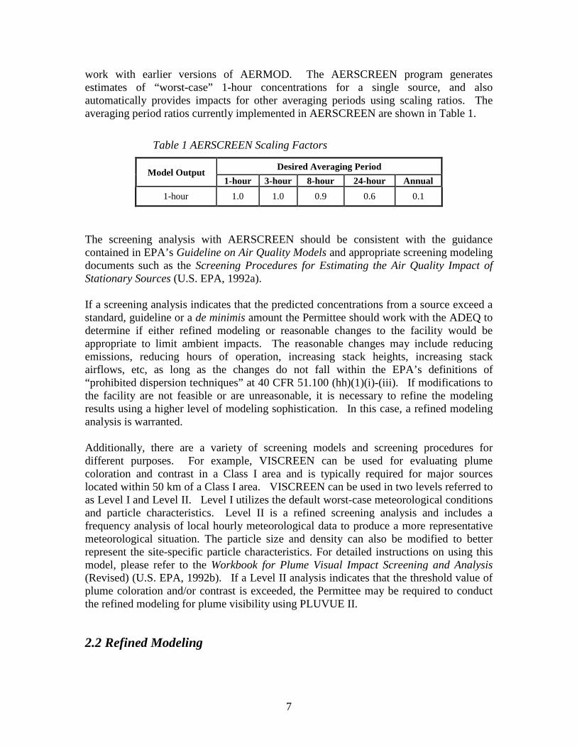
work with earlier versions of AERMOD. The AERSCREEN program generates estimates of “worst-case” 1-hour concentrations for a single source, and also automatically provides impacts for other averaging periods using scaling ratios. The averaging period ratios currently implemented in AERSCREEN are shown in Table 1.

Table 1 AERSCREEN Scaling Factors

Model Output Desired Averaging Period 1-hour 3-hour 8-hour 24-hour Annual

1-hour 1.0 1.0 0.9 0.6 0.1

The screening analysis with AERSCREEN should be consistent with the guidance contained in EPA’s Guideline on Air Quality Models and appropriate screening modeling documents such as the Screening Procedures for Estimating the Air Quality Impact of Stationary Sources (U.S. EPA, 1992a). If a screening analysis indicates that the predicted concentrations from a source exceed a standard, guideline or a de minimis amount the Permittee should work with the ADEQ to determine if either refined modeling or reasonable changes to the facility would be appropriate to limit ambient impacts. The reasonable changes may include reducing emissions, reducing hours of operation, increasing stack heights, increasing stack airflows, etc, as long as the changes do not fall within the EPA’s definitions of “prohibited dispersion techniques” at 40 CFR 51.100 (hh)(1)(i)-(iii). If modifications to the facility are not feasible or are unreasonable, it is necessary to refine the modeling results using a higher level of modeling sophistication. In this case, a refined modeling analysis is warranted. Additionally, there are a variety of screening models and screening procedures for different purposes. For example, VISCREEN can be used for evaluating plume coloration and contrast in a Class I area and is typically required for major sources located within 50 km of a Class I area. VISCREEN can be used in two levels referred to as Level I and Level II. Level I utilizes the default worst-case meteorological conditions and particle characteristics. Level II is a refined screening analysis and includes a frequency analysis of local hourly meteorological data to produce a more representative meteorological situation. The particle size and density can also be modified to better represent the site-specific particle characteristics. For detailed instructions on using this model, please refer to the Workbook for Plume Visual Impact Screening and Analysis (Revised) (U.S. EPA, 1992b). If a Level II analysis indicates that the threshold value of plume coloration and/or contrast is exceeded, the Permittee may be required to conduct the refined modeling for plume visibility using PLUVUE II.

2.2 Refined Modeling

7

ADEQ may determine that refined modeling is necessary if the results of the screening or refined screening analysis indicate that the predicted concentrations from a source exceed a standard, guideline, or a de minimis amount. Typically, it is the Permittee’s responsibility to perform refined modeling. However, ADEQ may perform this type of modeling under certain circumstances, such as for small businesses that cannot afford the costs associated with refined modeling or for other reasons. ADEQ will charge for these services through applicable permit fees. Before a refined modeling analysis is performed, it is highly recommended that the Permittee submit a written modeling protocol that describes the methodologies to be utilized in the modeling analysis and obtain written ADEQ approval before proceeding. AERMOD Refined modeling requires much more detailed inputs and complex models to calculate ambient impacts than screening modeling. The primary model used for the refined modeling of industrial sources is the most recent regulatory version of EPA’s AERMOD model. The AERMOD modeling system has replaced Industrial Source Complex 3 (ISC3) as the preferred recommended model for most regulatory modeling applications, as announced in Appendix W of 40 CFR Part 51 (U.S.EPA, 2005). Currently, the AERMOD model can be downloaded from EPA’s Support Center for Regulatory Air Models (SCRAM) website at http://www.epa.gov/ttn/scram AERMOD is a steady-state, multiple-source dispersion model that uses Gaussian or Non-Gaussian treatment depending on atmospheric conditions (Gaussian for stable conditions, non-Gaussian for unstable conditions). AERMOD is the EPA-preferred refined model for estimating impacts at receptors located in simple terrain and complex terrain (within 50 km of a source) due to emissions from industrial sources. AERMOD can predict ambient concentrations using onsite, representative, or worst-case meteorological data sets. AERMOD is capable of calculating downwind ground-level concentrations due to point, area, and volume sources and can accommodate a large number of sources and receptors. AERMOD can also handle line sources by simulating them as a series of area or volume sources. Starting with AERMOD version 12345, a new LINE source type has been included that allows users to specify line-type sources, as an alternative to the current area source type for rectangular sources. (Depending on the line source type that is being modeled, users may wish to model line sources as a series of volume sources, if appropriate.) AERMOD incorporates algorithms for the simulation of aerodynamic downwash induced by buildings. AERMOD handles flat terrain and complex terrain using a consistent approach, which is different from ISC3’s critical dividing streamline approach. As a result, users do not need to specify flat terrain (receptor elevation is less than final plume rise) or complex terrain (receptor elevation is higher than final plume rise). As long as the terrain elevations are appropriately assigned for sources and receptors, AERMOD will calculate concentrations for flat and complex terrain intrinsically. AERMOD does not handle atmospheric chemistry processes, except in a few circumstances (for example, the SO2 half-life for urban sources

8

as discussed in Section 3.7 and the NO2 chemistry as discussed in Section 7.1). Modeling involving pollutant transformations (i.e. ozone, sulfates, etc.) is not generally required for new or modified sources and is not addressed in this guidance document. In general, AERMOD should be run in the regulatory default mode. The Permittee may use the following non-default or beta options without justification:

• Plume Volume Molar Ratio Method (PVMRM) or Ozone Limiting Method (OLM) for NO2 modeling (see Section 7.1.3; note that the Permittee does need to justify which method is more suitable);

• Beta options for raincap stacks (POINTCAP) and horizontal stacks (POINTHOR) (see Section 3.3.8).

For using other non-default options or beta options, the Permittee should provide sufficient justification and get approval from ADEQ. For example, the latest version of AERMOD (version 12345) has incorporated two new beta (non-Default) options, LowWind1 and LowWind2, to address potential concerns regarding model performance under low wind speed conditions. If the Permittee believes that using such beta options is more appropriate for their case, it is the Permittee’s responsibility to demonstrate this and get approval by ADEQ. Otherwise, these beta options should not be used. CALPUFF The CALPUFF model is typically used to assess impacts at Class I areas. CALPUFF incorporates more sophisticated physics and chemistry and requires more extensive data input than AERMOD. CALPUFF is a multi-layer, multi-species non-steady-state puff dispersion model that simulates the effects of time- and space-varying meteorological conditions on pollution transport, transformation and removal. It includes algorithms for sub-grid scale effects (such as terrain impingement), as well as longer range effects (such as pollutant removal due to wet scavenging and dry deposition, chemical transformation, and visibility effects of particulate matter concentrations). The User’s Guide for the CALPUFF Dispersion Model (Earth Tech, 2000) provides more information on the CALPUFF model. The files associated with the CALPUFF system, e.g., executables/source code, preprocessors, associated utilities, test cases, selected meteorological data sets and documentation can be found on TRC’s website at http://www.src.com/calpuff/calpuff1.htm The EPA regulatory approved version of CALPUFF should always be used for regulatory applications unless otherwise approved by ADEQ and EPA. Currently, CALPUFF-Version 5.8 is the version of the modeling system officially approved by EPA. While CALPUFF can be applied on scales of tens to hundreds of kilometers, it is currently used for long range transport assessments (greater than 50 km but less than 300 km from the emission source). CALPUFF is not the EPA-preferred model for near-field (less than 50 kilometers) applications, but may be considered as an alternative model on a

9

case-by-case basis for near-field applications involving “complex winds” (U.S. EPA, 2008a). Any use of CALPUFF in the near-field must be thoroughly justified and approved by ADEQ and EPA. The basic requirements for justifying use of CALPUFF for near-field regulatory applications consist of three main components:

• Treatment of complex winds is critical to estimating design concentrations; • The preferred model (AERMOD) is not appropriate or less appropriate than

CALPUFF; and • Five criteria listed in paragraph 3.2.2(e) of the Guideline for use of CALPUFF as

an alternative model are adequately addressed.

3 MODELING ANALYSIS FEATURES This section provides an overview of the major components of a permit modeling analysis. Model user’s guides may also be useful in providing the Permittee detailed information regarding features of a modeling analysis. When in doubt, modeling questions should be presented to ADEQ for assistance.

3.1 Modeling Worst-Case Scenarios For each applicable pollutant and each applicable averaging time, a modeling analysis must consider worst-case scenarios based on evaluation of the following:

• Different operating modes of equipment (e.g. simple cycle and combined cycle for turbines),

• Various emission rates (normal steady-state operations, start-up and shutdown operations, emissions at various loads, spikes in short-term emissions, alternative fuels, etc.), and

• The effect of various operational loads on emission rates and dispersion characteristics, such as stack exit velocity.

Based on the evaluation, a worst-case scenario for each pollutant and averaging time can be selected as the basis for the modeling run.

3.1.1 Emissions Profiles The maximum short-term emission rates for each source should be used to demonstrate compliance with all short-term averaging standards and guidelines. If equipment is to be operated under different conditions, such as operating hours, load factor or fuel type, each emission scenario should be evaluated and the maximum short-term emission rate should be used. The emission profile should clearly describe the underlying factors from which the emissions are derived. For example, for dual-fuel combustion sources, the fuel-type that would generate the highest emissions should be modeled. Another example is for

10

gas turbines, which have different emissions and source parameters, such as exit velocity and exit temperature under different loads. This is further explained in Section 3.1.2. Some sources may have higher-than-normal emissions triggered by certain events. For example, high short-term emissions may result from startup/shutdown operations or bypasses of control equipment. For compliance demonstrations with the 1-hour NO2 or SO2 NAAQS, special consideration should be given to determine whether such emissions should be included in the modeling analysis or not. Because of the probabilistic nature of the two standards, EPA recommends that the most appropriate data to use for compliance demonstrations for the 1-hour NO2 and SO2 standards are those based on emissions scenarios that are continuous enough or frequent enough to contribute significantly to the annual distribution of maximum daily 1-hour concentrations. Therefore, ADEQ may allow an exemption from 1-hour NO2 and SO2 modeling if these events are infrequent enough so that the emissions caused by these events will not contribute significantly to the annual distribution of maximum daily 1-hour concentrations (see Section 7.1.6). As the exemption determination is on a case-by-case basis, the Permittee should provide ADEQ detailed information about these events such as frequency and duration (see Section 7.1.6). Based on Appendix W Section 8.1.2.a - footnote a (U.S. EPA, 2005), modeling emissions due to malfunction is not required unless the emissions are the result of poor maintenance, careless operation, or other preventable conditions. For compliance demonstrations with the 24-hour or annual NAAQS, emission rates modeled should incorporate a suitable number of these high-emission periods combined with normal equipment operations. For example, power generation facilities are typically permitted for a certain number of startup/shutdown events. Therefore, calculations for 24-hour average emissions or annual emissions for a power generation facility must consider the emissions from startup/shutdown events combined with emissions from steady-state operations. It is important that the Permittee provide emissions information for all averaging times to be considered in the modeling analysis. Potential short-term emissions “spikes” from highly fluctuating short-term emissions sources (such as some types of kilns) also need to be characterized and considered in the modeling analysis.

Emissions from equipment used during emergency conditions, such as fire pumps to provide water in responding to fires and emergency generators to provide power during the unexpected interruption of electrical service from the utility, are generally not required in compliance modeling. However, emissions from routine testing or maintenance on such emergency equipment should be included, unless the sources fall within the definition of “intermittent sources” that can be exempted from 1-hour modeling for compliance demonstration (see Section 7.1.6).

3.1.2 Load Analyses A load analysis is also required for equipment that may operate under a variety of conditions that could affect emission rates and dispersion characteristics. A load

11

analysis is a preliminary modeling exercise in which combinations of parameters (e.g. ambient temperature, sources loads, relative humidity, etc.) are analyzed to determine which combination leads to the highest modeled impact. For example, turbines should be evaluated at varying loads and temperatures to determine the worst-case modeled impacts. Furthermore, cold temperature conditions at the site also should be considered. The GAQM provides further guidance on conducting a load analysis and recommends that at a minimum, load analyses should be conducted at 100%, 75% and 50% capacity. However, each Permittee can choose the load factors that are most representative of their own operating conditions. The stack parameters of various load levels that result in the highest impact should be used in compliance demonstration.

3.1.3 Emission Caps Some facilities may wish to accept facility-wide emissions caps for a particular pollutant. However, emissions of these pollutants may exhaust into the atmosphere through various stacks. Different stacks with different dispersion parameters may result in significantly different ambient impacts, especially in complex terrain. Many operational possibilities exist under a proposed facility-wide cap. To adequately evaluate the ambient impacts of variable emissions of pollutants with facility-wide caps, the Permittee needs to consider several operational scenarios. For example, assume that two stacks, Stack A and Stack B, have very different dispersion differences (i.e. different stack heights, airflows, and exhaust diameters). Assume that Stack A typically emits 25% of the emissions and Stack B emits 75% of the emissions from the throughput in a single production unit. Assume that it is possible to configure the production unit so that Stack A is bypassed and all of the emissions exhaust through Stack B (and vice versa). Under this scenario, the Permittee should consider the following modeling scenarios in addition to the aforementioned typical operating scenario: (a) 100% of emissions through Stack A only, (b) 100% of emissions through Stack B only, and (c) 50% of emissions through Stack A and 50% of emissions through Stack B. In other words, the Permittee needs to determine and separately present worst-case modeled impacts resulting from various operating scenarios, since a facility-wide cap would allow for such operational flexibility. These analyses are intended to demonstrate that the health and welfare of the public will be protected from all potential operating scenarios of a proposed project.

3.2 Modeling Emissions Inventory A modeling emissions inventory may consist of the emission points of the sources to be permitted, as well as other applicable onsite and offsite sources. An organized emissions inventory provides a crucial link between the emissions used to determine source applicability and the emissions used directly in the modeling analysis. Permittees are required to calculate emissions for proposed projects and compare these values to trigger thresholds for PSD applicability, Maximum Achievable Control Technology (MACT) applicability, etc. Typically, these emissions calculations are presented as annual

12

emissions with units of ton/yr. On the other hand, modeling analyses typically utilize emission rates with units of lb/hr or g/sec. The averaging periods over which ambient standards and guidelines apply vary depending upon pollutant type. For example, emissions over 1-hour and 8-hour periods would be needed to compare the ambient impact of carbon monoxide emissions with the 1-hour and 8-hour standards for carbon monoxide. For sulfur dioxide, short-term ambient standards are in terms of 1-hour and 3-hour averaging periods. For nitrogen dioxide, the short-term ambient standard is in terms of a 1-hour averaging period. Emission inventories should be tabulated for all different averaging periods applicable to pollutants emitted from a facility. To expedite ADEQ’s review of the permit application and associated modeling analyses, it is suggested that the Permittee calculates lb/hr, ton/yr, and g/s emission rates for all averaging times in the same (or similar) tables. These emissions tables should also include operational limits (hr/day, hr/yr) and production material throughputs and/or unit ratings for each emission source. Emissions units are typically considered on a production unit basis while modeling requires the consideration of exhaust points. It is possible to have several production units that exhaust to a common exhaust point. Therefore, emissions should be presented in the permit application so that it is possible to determine source applicability while also clearly indicating the calculations utilized to determine modeled emission rates for each exhaust point at the facility.

3.3 Types of Sources Regulatory modeling should reflect the actual characteristics of the proposed emission sources. Several different source types used to characterize emissions releases are described in this section.

3.3.1 Point Sources The point source is the most common type of source that is modeled in permit modeling analyses. Emissions from point sources are released to the atmosphere through well-defined stacks, chimneys, or vents. The following stack parameters are needed to model point sources:

• Emission rate in g/s, • Stack inside diameter in meters, • Stack height above grade in meters, • Stack gas exit velocity in m/s, • Stack gas exit temperature in degrees K.

Since the AERMOD model uses direction-specific building dimensions for all sources subject to building downwash, there are no building parameters entered on the source parameters (SRCPARAM) card. Building dimensions are entered on the building’s

13

dimensions card. If “0.0” is input for the stack exit temperature, AERMOD adjusts the hourly exit temperature to be equal to the ambient temperature. This allows the user to model a plume released at ambient temperature. If a negative constant is input for the exit temperature, AERMOD will adjust the exit temperature to be equal to the ambient temperature plus the absolute value of that constant. AERMOD currently does not have the capability to model plumes with an exit temperature below the ambient temperature.

3.3.2 Volume Sources Volume sources are used to model releases from a variety of industrial sources such as building roof monitors, multiple vents, conveyor belts, roads, drop points from loaders, and material storage piles. Moreover, line sources (e.g. road emission sources as described in Sec. 3.3.5) have long been recommended to be modeled as a series of volume sources. The following parameters are needed to model volume sources:

• Emission rate in g/s, • Source release height (center of volume) above ground (he) in meters, • Initial lateral dimension of the volume (σyo) in meters, • Initial vertical dimension of the volume (σzo) in meters.

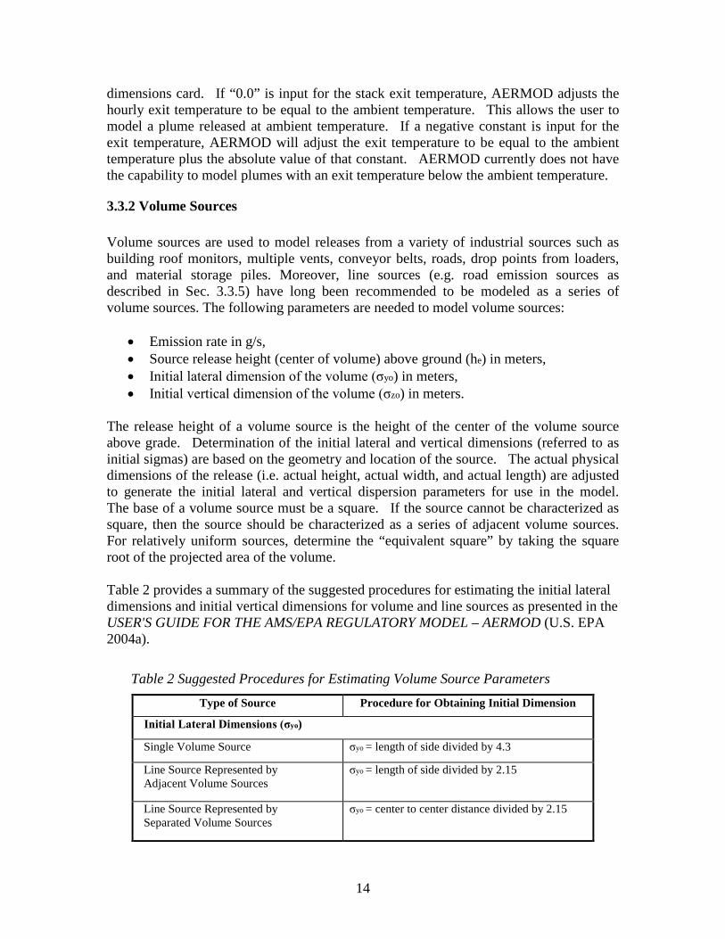
The release height of a volume source is the height of the center of the volume source above grade. Determination of the initial lateral and vertical dimensions (referred to as initial sigmas) are based on the geometry and location of the source. The actual physical dimensions of the release (i.e. actual height, actual width, and actual length) are adjusted to generate the initial lateral and vertical dispersion parameters for use in the model. The base of a volume source must be a square. If the source cannot be characterized as square, then the source should be characterized as a series of adjacent volume sources. For relatively uniform sources, determine the “equivalent square” by taking the square root of the projected area of the volume. Table 2 provides a summary of the suggested procedures for estimating the initial lateral dimensions and initial vertical dimensions for volume and line sources as presented in the USER'S GUIDE FOR THE AMS/EPA REGULATORY MODEL – AERMOD (U.S. EPA 2004a).

Table 2 Suggested Procedures for Estimating Volume Source Parameters Type of Source Procedure for Obtaining Initial Dimension

Initial Lateral Dimensions (σyo)

Single Volume Source σyo = length of side divided by 4.3

Line Source Represented by Adjacent Volume Sources

σyo = length of side divided by 2.15

Line Source Represented by Separated Volume Sources

σyo = center to center distance divided by 2.15

14

Initial Vertical Dimensions (σzo)

Surface-Based Source (he ~ 0) σzo = vertical dimension of source divided by 2.15

Elevated Source (he > 0) on or Adjacent to a Building

σzo = building height divided by 2.15

Elevated Source (he > 0) not on or Adjacent to a Building

σzo = vertical dimension of source divided by 4.3

3.3.3 Area Sources Area source algorithms are used to model low level or ground level releases with no plume rise such as storage piles, slag dumps, and lagoons. The AERMOD model uses a numerical integration approach for modeling impacts from area sources. AERMOD includes three options for specifying the shape of an area source:

• AREA – for rectangular areas that may also have a rotation angle specified to a north-south orientation. The parameters needed are: 1) area emission rate in g/(s-m2), 2) source release height above ground in meters, 3) length of X side of area in meters, 4) length of Y side of area in meters, and 5) optional inputs of orientation angle in degrees and initial vertical dimension of the area source plume in meters.

• AREAPOLY – area of an irregularly shaped polygon of up to 20 sides. The necessary input parameters are: 1) area emission rate in g/(s-m2), 2) source release height above ground in meters, 3) number of vertices, 4) coordinates of each vertex and 5) an optional initial vertical dimension of the plume in meters.

• AREACIRC – for circular shaped area sources The necessary input parameters are 1) area emission rate in g/(s-m2), 2) source release height above ground in meters, 3) radius of circular area in meters and number of vertices (AERMOD will automatically approximate the area of the circle as the area of a polygon with 20 vertices if this is omitted), and 4) an optional initial vertical dimension of the plume in meters.

The performance stability of the numerical integration algorithm for area sources may strongly depend on the aspect ratio (i.e., length/width). An aspect ratio upper limit of 10:1 was initially used as a criterion for issuing a non-fatal warning message in the earliest versions of AERMOD. Starting with AERMOD Version 09292, EPA has modified the criterion from an aspect ratio of 10:1 to an aspect ratio of 100:1, stating that a ratio of 10:1 is probably too strict and may unnecessarily lead to a large number of warning messages in some cases. However, it should be addressed that the upper limit of aspect ratio for stable performance of the numerical integration algorithm for area sources has not been fully tested and documented. Therefore, the Permittee should always check to ensure that the aspect ratio used is appropriate.

15

It should also be noted that the emission rate for the area source is an emission rate per unit area, which is different than the point and volume source emission rates, which are total emissions for the source.

3.3.4 Line Sources Starting with AERMOD version 12345, a new LINE source type has been included that allows users to specify line-type sources based on a start-point and end-point of the line and the width of the line, as an alternative to the current AREA source type for rectangular sources. The LINE source type utilizes the same routines as the AREA source type, and will give identical results for equivalent source inputs. The LINE source type also includes an optional initial sigma-z parameter to account for initial dilution of the emissions. As with the AREA source type, the LINE source type does not include the horizontal meander component in AERMOD. Since the LINE source type includes both start and endpoints, an issue has been raised regarding inclusion of LINE source type in AERMAP, the terrain processor for AERMOD (i.e., what reference point to use in AERMAP). Until this issue is clarified, the Permittee should avoid using the LINE source type.

3.3.5 Road Emission Sources ADEQ requires modeling of fugitive road dust for both short-term and annual averaging periods. Road emissions can be represented as a series of volume sources. ADEQ follows the volume source technique recommended by EPA’s Haul Road Workgroup for modeling haul road emissions (Haul Road Workgroup, 2011). The permit modeling analysis must include road emissions if they will be generated in association with transport, storage, or transfer of materials (raw, intermediate, and waste), including sand, gravel, caliche, or other road-based aggregates. To represent road emissions by volume sources, follow the eight steps described in the following paragraphs. Volume Step 1: Determine the adjusted width of the road. For single-lane roadways, the adjusted width is the vehicle width plus 6 meters. For two-lane roadways, the adjusted width is the actual width of the road plus 6 meters. The additional width represents turbulence caused by the vehicle as it moves along the road. This width will represent a side of the base of the volume. Volume Step 2: Determine the number of volume sources, N. Divide the length of the road by the adjusted width. The result is the maximum number of volume sources that could be used to represent the road. Volume Step 3: Determine the height of the volume. The height will be equal to 1.7 times the height of the vehicle generating the emissions.

16

Volume Step 4: Determine the initial horizontal sigma (σyo) for each volume.

• If the road is represented by a single volume source, divide the adjusted width by 4.3.

• If the road is represented by adjacent volume sources, divide the adjusted width by 2.15.

• If the road is represented by alternating volume sources, divide twice the adjusted width – measured from the center point of the first volume to the center point of the next represented volume – by 2.15. Start with the volume source nearest the process area boundary. This representation is often used for long roads.

Volume Step 5: Determine the initial vertical sigma (σzo). Divide the height of the volume determined in Step 3 by 2.15. Volume Step 6: Determine the release height. Divide the height of the volume by two. This point is the center of the volume. Volume Step 7: Determine the emission rate for each volume used to calculate the initial horizontal sigma in Step 4. Divide the total emission rate equally among the individual volume sources used to represent the road, unless there is a known spatial variation in emissions. Volume Step 8: Determine the UTM coordinate (See Section 3.5) for the release point. The release point location is in the center of the projected area of the volume. This location must be at least one meter from the nearest receptor. For cases where volume sources cannot be used due to ambient air receptors being located in the volume source exclusion zone, road emissions can be modeled as area sources with:

• Length – length of roadway segment (Aspect ratio in AERMOD extended to 100:1 before warning);

• Top of plume, release height, plume width, and Sigma Z set to values listed above for volume sources;

• Emission rate in grams/second/m2

3.3.6 Flares Flares are typically modeled in either standard mode or event mode. In standard mode, the pilot gas, purged gas or assist gas is burning at relatively low intensity - a small flame is usually present. In event mode, the flare is burning during temporary startup, shutdown, maintenance of a process or control unit - a large flame is present, with intense heat release and buoyancy.

17

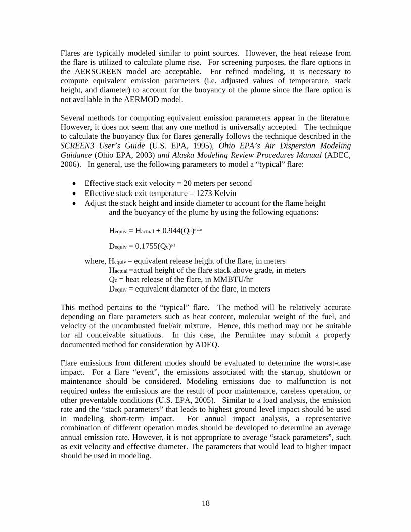
Flares are typically modeled similar to point sources. However, the heat release from the flare is utilized to calculate plume rise. For screening purposes, the flare options in the AERSCREEN model are acceptable. For refined modeling, it is necessary to compute equivalent emission parameters (i.e. adjusted values of temperature, stack height, and diameter) to account for the buoyancy of the plume since the flare option is not available in the AERMOD model. Several methods for computing equivalent emission parameters appear in the literature. However, it does not seem that any one method is universally accepted. The technique to calculate the buoyancy flux for flares generally follows the technique described in the SCREEN3 User’s Guide (U.S. EPA, 1995), Ohio EPA’s Air Dispersion Modeling Guidance (Ohio EPA, 2003) and Alaska Modeling Review Procedures Manual (ADEC, 2006). In general, use the following parameters to model a “typical” flare:

• Effective stack exit velocity = 20 meters per second • Effective stack exit temperature = 1273 Kelvin • Adjust the stack height and inside diameter to account for the flame height

and the buoyancy of the plume by using the following equations:

Hequiv = Hactual + 0.944(Qc)0.478

Dequiv = 0.1755(Qc)0.5

where, Hequiv = equivalent release height of the flare, in meters Hactual =actual height of the flare stack above grade, in meters Qc = heat release of the flare, in MMBTU/hr Dequiv = equivalent diameter of the flare, in meters

This method pertains to the “typical” flare. The method will be relatively accurate depending on flare parameters such as heat content, molecular weight of the fuel, and velocity of the uncombusted fuel/air mixture. Hence, this method may not be suitable for all conceivable situations. In this case, the Permittee may submit a properly documented method for consideration by ADEQ. Flare emissions from different modes should be evaluated to determine the worst-case impact. For a flare “event”, the emissions associated with the startup, shutdown or maintenance should be considered. Modeling emissions due to malfunction is not required unless the emissions are the result of poor maintenance, careless operation, or other preventable conditions (U.S. EPA, 2005). Similar to a load analysis, the emission rate and the “stack parameters” that leads to highest ground level impact should be used in modeling short-term impact. For annual impact analysis, a representative combination of different operation modes should be developed to determine an average annual emission rate. However, it is not appropriate to average “stack parameters”, such as exit velocity and effective diameter. The parameters that would lead to higher impact should be used in modeling.

18

3.3.7 Open Pit Sources Open pit algorithms are used to model particulate emissions from open pits, such as surface copper mines and rock quarries. These algorithms simulate emissions that initially disperse in three dimensions with little or no plume rise. Open pit algorithms are available in AERMOD, which essentially adopts the ISC3 open pit algorithm. In the AERMOD model, the open pit algorithm uses an effective area for modeling pit emissions based on meteorological conditions. The algorithm then utilizes the numerical integration area source algorithm to model the impact of the emissions from the effective area sources. The following parameters are needed to model open pit sources: open pit emission rate (emission rate per unit area), average release height above the base of the pit, the initial length and width of the pit, and the volume of the pit. An optional input is “ANGLE,” which specifies the orientation angle for the rectangular open pit in degrees from North, measured positive in clockwise direction (Addendum User’s Guide for the AMS/EPA Regulatory Model – AERMOD, U.S.EPA, 2004a).

3.3.8 Pseudo Point / Non-Standard Point Source Pseudo point sources may be used to represent vent emissions, such as those from storage tanks. Typically such releases occur at ambient temperature and with little driving force. Consequently, these releases are characterized with minimal momentum and buoyancy. The configuration of these sources must reflect these characteristics by adjusting the stack parameters. The Texas Commission on Environmental Quality (TCEQ) provides a method to model pseudo point sources (TCEQ, 1999). If it is necessary to model emissions from fugitive sources and if a pseudo-point characterization is appropriate, then the Permittee can use the following modeling parameters:

• Stack exit velocity = 0.001 meters per second • Stack exit diameter = 0.001 meter • Stack exit temperature = 0 Kelvin (causes the AERMOD model to use the

ambient temperature as the exit temperature) • Actual release height

It is suggested that the Permittee provide ADEQ with details regarding the pseudo point sources for review prior to modeling. Non-standard point sources include non-vertical stacks or vertical stacks with obstructed emissions (such as a raincap). Currently, AERMOD includes two beta options for raincap stacks (POINTCAP) and horizontal stacks (POINTHOR). ADEQ will accept the use of these beta options until an EPA approved alternative method for modeling non-vertical and/or obstructed emissions is accepted. To use these beta options, the user should input actual stack parameters, including exit velocity, exit temperature and stack diameter. The source location should be given in the same way as for standard point

19

sources. AERMOD will apply internal adjustments to the stack parameters for plume rise and stack-tip downwash. For horizontal releases, AERMOD assumes that the release is oriented with the wind direction. For PRIME-downwash sources, the user-specified exit velocity for horizontal releases is treated initially as horizontal momentum in the downwind direction. For detailed guidance, please refer to the AERMOD Implementation Guide Section 6.1 (U.S. EPA, 2009a).

3.3.9 Emission Point Collocation Regulatory modeling should reflect the actual characteristics of the proposed or existing emissions points at a facility. Therefore, emission points should not be co-located except in well-justified situations. For example, collocation may be appropriate when the number of emission points at a large facility exceeds the capability of the model. It is not acceptable to co-locate emission points merely for convenience or to reduce model run time. Collocating emission points may be appropriate if individual emission points:

• Emit the same pollutant(s), • Have the same source release parameters, and • Are located within 100-meters of each other.

For very large emission sources such as power plants and copper smelters, ADEQ does not allow co-location of individual emission points since slight movements in the location of large emission points can significantly impact modeling results for NAAQS, PSD increment, and visibility analyses. It is suggested that the Permittee provides ADEQ details regarding the possible co-location of emission points for review prior to modeling.

3.4 Ambient Air Boundary The ambient air boundary must be determined before an ambient air assessment can be completed. Permit Permittees are required to demonstrate modeled compliance with NAAQS or PSD increments at receptors spaced along and outside the ambient air boundary (Section 3.6). The recent revised NAAQS for NO2, SO2, PM10 and PM2.5 are significantly more stringent than the previous standards and in conjunction with EPA ambient air policy will provide protection of the public health previously afforded by the process area boundary (PAB) policy. Therefore, ADEQ has determined that the EPA’s ambient air policy will be incorporated into this guidance for modeling purposes. 40 CRF Part 50.1(e) defines ambient air as, “…that portion of the atmosphere, external to buildings, to which the general public has access.” A letter dated December 19, 1980, from EPA’s Administrator Douglas Costle to Senator Jennings Randolph, has stated that “the exemption from ambient air is available only for the atmosphere over land owned or controlled by the source and to which public access is precluded by a fence or other physical barriers”. The Regional Meteorologists’ memorandum has further stated that

20

“…for modeling purposes the air everywhere outside of contiguous plant property to which public access is precluded by a fence or other effective physical barrier should be considered in locating receptors” (U.S. EPA,1985). Based on these definitions and guidance, ADEQ has developed the following guidance to be used when determining the ambient air boundary for a facility.

3.4.1 Definition of General Public

According to EPA, the general public includes “anyone who is not employed by or under control of the facility, but, more specifically, persons who do not require the facility’s permission to be on the property” (U.S. EPA, 2007). The general public may not include mail carriers, equipment and product suppliers, maintenance and repair persons, as well as persons who are permitted to enter restricted land for the business benefit of the person who has the power to control access to the land. Therefore, ADEQ does not consider individuals who in some way interact with or participate in a source’s activities to be part of the general public. Such individuals would include, for example, the owner/operator and its employees, contractors and their employees, vendors and support businesses and their employees, and government agencies and services and their employees.

EPA has further clarified that the general public should include (U.S. EPA, 2007):

• Customers of a business to which access is typically not restricted during business hours. For example, the customer of a restaurant or other retail business is a member of the general public even if the proprietor restricts public access during non-business hours by locking the entrance to the property.

• Persons who are frequently permitted to enter restricted-access land for a purpose that does not ordinarily benefit the “business.” For example, EPA has treated athletic facilities within the restricted fence line of a source as ambient air when persons unconnected to the business were regularly granted access for sporting events (which do not necessarily benefit a business).

3.4.2 Public Access If general public access is effectively precluded by a fence or other physical barriers, the facility is assumed to be controlled and public access effectively precluded, and the ambient air boundary can be set at where the fence line or other physical barriers are located. However, a fence or other physical barriers that are not sufficient to preclude public access should not be used for determining the ambient air boundary. For example, EPA has indicated that a three-strand barb-wire fence may not be adequate to keep the general public off a farm land (U.S. EPA, 2000a). In addition to fences or other human-made barriers, natural physical barriers may be used as a portion of the ambient air boundary. For example, EPA has indicated that a riverbank can form a natural barrier such that fencing is not necessary (U.S. EPA, 1987a). Such natural barriers should, however, be clearly posted and regularly patrolled by plant

21

security. It should be addressed that, rugged terrain or a water body should not be automatically considered as an effective natural barrier unless the Permittee adequately demonstrates and documents that public access can be effectively precluded. Any public roads will be considered as ambient air. Any streams or rivers transecting a property will be considered as ambient air unless the Permittee adequately demonstrates and documents that public access can be legally precluded.

3.4.3 Property without an Effective Fence or Other Physical Barriers If the facility does not have a fence or other physical barriers to preclude general public access effectively, then ADEQ will accept the use of the facility’s Process Area Boundary (PAB) as the ambient air boundary. The PAB is defined as the process areas within the facility occupied by emission generating activities, the area in the immediate vicinity of those activities and the area between adjacent activities. If the Permittee does not wish to use the PAB as the ambient air boundary, the Permittee should conduct a case-by-case analysis demonstrating that the general public’s access to areas other than the PAB is effectively prevented. ADEQ recommends Permittees discuss their approach to such a case-by-case analysis with department staff before submitting a modeling protocol.

3.4.4 Leased Property Interpretation of ambient air in situations involving leased land is usually complicated. ADEQ should be consulted regarding any specific case involving leased property as it affects the ambient air boundary determination. Because determining the ambient air boundary is a somewhat subjective exercise involving input from both the Permittee and ADEQ, the Permittee should provide ADEQ with a scaled facility plot plan or aerial photo clearly indicating the proposed ambient air boundary prior to performing the modeling analysis. If the Permittee submits a modeling protocol to ADEQ, the protocol should include a discussion of the ambient air boundary.

3.5 Modeling Coordinate Systems Refined modeling should always be performed using Universal Transverse Mercator (UTM) coordinates. Please do not use coordinate systems based on plant coordinates. Always indicate the datum used for the UTM coordinates. There are several horizontal data coordinate systems (NAD27, WGS72, NAD83, and WGS84) that are used to represent locations on the earth’s surface. Make sure that all coordinates are generated from a common horizontal datum when representing receptor, building, and source locations.

22

It is necessary to use UTM coordinates to be consistent with emission point locations provided on permit application forms and other reference materials such as USGS topographic maps. In addition, ADEQ utilizes UTM information to check submitted modeling files against digital GIS mapping products.

3.6 Receptor Networks Receptors should be placed throughout a modeling domain to determine areas of maximum predicted concentrations. The extent of receptor coverage around a facility is usually handled on a case-by-case basis since source dispersion characteristics, topography, and meteorological conditions differ from source to source. Table 3 indicates typical receptor spacing suggested by ADEQ for modeling analyses. AERMOD has a maximum allowed number of receptors set at 50,000. Additional modeling should be conducted in the vicinity of each receptor when a predicted concentration exceeds 90% of an applicable standard or guideline. For example, use a tight grid with receptors spaced at 25 meters to fill in the fine, medium, or coarse receptors that indicate a predicted concentration greater than 90% of an applicable standard or guideline. The furthest extent and spacing of receptors away from the ambient air boundary should be evaluated on a case-by-case basis. In the modeling protocol, the Permittee should provide a justification as to the extent and spacing of receptors. In some circumstances, ADEQ may require a receptor network coverage of 50 km, even if the maximum impact from the proposed project is expected to occur near the project site. One common example of such a circumstance would be a project that would cause a significant public concern.

Table 3 Suggested Receptor Spacing

Type of Receptors Suggested Receptor Spacing (meters) Receptor Coverage Area

Tight 25 Along ambient air boundary (AAB)

Fine 100 From AAB to 1 km Medium 200 - 500 From 1 km to 5 km away from AAB Coarse 500 - 1,000 From 5 km to 20 km away from AAB

Very Coarse 1,000-2,500 From 20 km to 50 km away from AAB

Discrete Not Applicable Place at areas of concern such as nearby residences, schools, worksites or daycare

centers Non-Attainment Area Case-by-Case Discuss with ADEQ prior to modeling

Class I and Class II Wilderness Area Case-by-Case Discuss with Federal Land Manager prior to

modeling

23

Given the diverse topography of Arizona, most modeling domains include topography above stack height (i.e. complex terrain). Therefore, ADEQ typically requests that refined modeling be performed with elevations included for each receptor. Receptor elevations should be derived using AERMAP, the terrain processor of AERMOD. AERMAP produces terrain base elevations for each receptor and source, and hill height for each receptor. Prior to 2009, AERMAP utilized bilinear interpolation of regularly spaced nodes as in the two-dimensional U.S. Geological Survey (USGS) Digital Elevation Model (DEM) files. Beginning with version 09040, AERMAP has been revised to support processing of terrain elevations from the National Elevation Dataset (NED) in GEO-TIFF format. As DEM data will no longer be updated while NED data are being actively supported and checked for quality, NED represents a more up-to-date and improved resource for terrain elevations for use with AERMAP. Therefore, permit Permittees are encouraged to use NED data instead of DEM data. AERMAP currently does not support processing of elevation data in both the DEM format and the GeoTIFF format for NED data in the same run. After April 2013, the USGS National Map Server no longer offers download of NED data in GeoTIFF format, which is the format accepted by AERMAP. The server now only provides NED data in ArcGrid and GridFloat formats. To deal with this issue, Permittees may download the GeoTIFF NED data from the website of Multi-Resolution Land Characteristics (MRLC) Consortium Viewer, http://www.mrlc.gov/viewerjs/. Another option is to use GIS tools to convert GridFloat format into GeoTIFF format. It is critical that the terrain processor derive receptor and source elevations on a consistent coordinate system. For example, DEM files could refer to different horizontal datums. A 7.5 minute DEM file refers to either the NAD27 or NAD83 datum; and a one-degree DEM file refers to either the WGS72 or WGS84 datum. More recent DEM files have the record of the reference horizontal datum in the file header, which is read by AERMAP. AERMAP then converts the coordinates in the DEM file to a horizontal datum specified for the modeling domain. Older DEM files that are absent of such record will be read by AERMAP assuming that 7.5 minute DEM files refer to NAD27 and one-degree DEM files refer to WGS72. The Permittee should refer to the User’s Guide for the AERMOD Terrain Preprocessor (AERMAP) (U.S. EPA, 2004b) and the User’s Guide for the AERMOD Terrain Preprocessor (AERMAP) Addendum (U.S. EPA, 2004c) for detailed instruction of using the AERMAP program.

3.7 Rural/Urban Classification It is important to determine whether a source is located in an urban or rural dispersion environment. In general, urban areas cause greater rates of dispersion because of increased turbulent mixing and buoyancy-induced mixing. This mixing is due to the combination of greater surface roughness induced by the presence of many buildings and

24

structures and increased amounts of heat released from concrete and similar building materials. AERMOD has two keyword switches for turning on the urban mode: the URBANOPT keyword on the CO pathway and the URBANSRC keyword on the SO pathway. AERMOD enhances the turbulence for urban nighttime conditions more than what would be expected at adjacent rural locations. AERMOD also uses population estimates as a surrogate to define the magnitude of the differential heating caused by the urban heat island effect. It is worth pointing out that AERMOD incorporates the 4-hour half-life for modeling ambient SO2 concentrations in urban areas under the regulatory default option. EPA guidance identifies two procedures to make an urban or rural classification for dispersion modeling: the land-use procedure and the population density procedure. Both procedures require the evaluation of characteristics within a 3-kilometer radius from a facility. Of the two procedures, the land-use procedure is preferred. The land-use procedure specifies that the land-use within a three-kilometer radius of the source should be determined using the typing scheme developed by Auer (1978). If the sum of land use types I1 (heavy industrial), I2 (light to moderate industrial), C1 (commercial), R2 (compact residential-single family), and R3 (compact residential-multiple family) is greater than or equal to 50% of the area within the circle, then the area should be classified as urban. Otherwise the area should be classified as rural. Table 4 indicates Auer’s land-use categories. Unless the source is located in an area that is distinctly urban or rural, the land use analysis should provide the percentage of each land use type from the Auer scheme and the total percentages for urban versus rural. The latest available United States Geological Survey (USGS) topographic quadrangle maps in the vicinity of the facility should be used in this analysis. In some circumstances, such as in an area undergoing rapid development, county or local planning board maps may need to be used. For most applications, the Land Use Procedure described above is sufficient for urban/rural determination. However, cautions must be taken to apply the land use procedure under some special circumstances (U.S. EPA, 2009a). For example, the Auer’s land use analysis may result in a rural designation when sources are located within an urban area but located close enough to a large body of water or to other non-urban land use categories. In such cases, the Permittee should consider the potential for urban heat island influences across the full modeling domain. While these sources are defined as rural based on the land use procedure, an urban designation may be more appropriate, since the urban heat island is not a localized effect but is more regional in character. Another example is that stacks are located within or adjacent to small to moderate size urban areas but the plume may extend above the urban boundary layer height. In such cases, it is not appropriate to use the urban option in AERMOD since the application of the urban option may artificially limit the plume height. The determination of whether these sources should be modeled separately without the urban option will depend on a comparison of the stack height or effective plume height with the urban boundary layer height.

25

26

Table 4 Auer Land -Use Classifications

Auer Type Description Urban or

Rural?

I1 Heavy Industrial Urban

I2 Light-Moderate Industrial Urban

C1 Commercial Urban

R1 Common Residential (normal easements) Rural

R2 Compact Residential (single family) Urban

R3 Compact Residential (multiple family) Urban

R4 Estate Residential (multi-acre) Rural

A1 Metropolitan Natural Rural

A2 Agricultural Rural Rural

A3 Undeveloped (grasses) Rural

A4 Undeveloped (heavily wooded) Rural

A5 Water Surfaces Rural

3.8 Meteorological Data ADEQ recognizes that the availability of meteorological data in Arizona is limited. EPA’s Support Center for Regulatory Air Models (SCRAM) website http://www.epa.gov/ttn/scram, provides some meteorological data for Arizona which can be used in dispersion models. Additional data from the National Weather Service (NWS) (collected from 20+ sites in AZ) can be obtained from the National Climatic Data Center (NCDC) website at http://www.ncdc.noaa.gov. Upper-air data is also available from this site for select locations including Tucson, Flagstaff, Yuma and Winslow. In some cases, ADEQ allows the use of upper-air data from Desert Rock, Nevada and Albuquerque, New Mexico. Preprocessed, AERMOD-ready, meteorological data files are currently available for 16 meteorological sites across Arizona (Figure 1). ADEQ will maintain and update the existing processed AERMOD-ready meteorological database. ADEQ is planning to create a meteorological data website, from which Permittees can access all meteorological data files as well as associated technical support documents. For further information and discussion regarding representativeness of the data for the area of interest, please contact ADEQ modeling staff.

27

Figure 1 Locations of ADEQ AERMET Meteorological Data Sets

ZONE 1-4 AZ Climate Zones

▲ ADEQ AERMET Meteorological Sites

28

3.8.1 Meteorological Data Description and Rationale Appendix W states in Section 8.3.1.1 that the user should acquire enough meteorological data to ensure that worst-case conditions are adequately represented in the model results. Appendix W states that 5 years of NWS meteorological data or at least one year of site-specific data should be used(Section 8.3.1.2, Appendix W) and should be adequately representative of the study area. Given the complex topography of Arizona and the remote locations of many facilities from population centers, existing meteorological data is often not representative of meteorological conditions at these facilities. If on-site meteorological data is unavailable for a given facility and the Permittee wishes to model using meteorological data available from another location, the Permittee must submit a detailed meteorological analysis to ADEQ for review. The meteorological analysis should explain how meteorological data from an offsite location is representative of the meteorological patterns around the facility. The Permittee should discuss the differences/similarities in topography, climatology (especially wind patterns and mixing heights), and surface characteristics (surface roughness length, albedo, and Bowen ratio) between the two locations. The Permittee should also explain why the utilization of offsite meteorological data would provide conservative modeling results. If it is determined that representative meteorological data are not available, it will be necessary for the Permittee to collect at least one (1) year of site-specific data. To generate a model-ready meteorological data set, the Permittee merges monitored surface data with available upper-air data. At the earliest stages of the air quality permitting process, it is important that the Permittee communicate with ADEQ so that it can be determined whether or not meteorological monitoring will be necessary. If meteorological monitoring is necessary, the monitoring should follow monitoring guidance and QA/QC guidance from USEPA. ADEQ relies upon the guidance provided in the document, Meteorological Monitoring Guidance for Regulatory Modeling Applications (U.S. EPA, 2000b). ADEQ relies upon the QA/QC guidance provided in EPA’s Quality Assurance Handbook for Air Pollution Measurement Systems (five volume set). If on-site meteorological monitoring is required, the following variables should be measured:

• Wind direction and wind speed at appropriate levels to characterize dispersion and transport of source emissions. Wind measurements should not be made lower than 10 meters above grade.

• Ambient temperature at 2 meters above grade • Vertical temperature gradient • Incoming solar radiation (insolation) or net solar radiation • Pressure (optional but recommended) • Precipitation (optional but recommended) • Humidity (optional but recommended)

29

In some cases, an upper air monitoring with a SoDAR (Sonic Detection And Ranging) device may be required for collecting additional wind profile over the range of emission release and final plume heights.

3.8.2 Meteorological Data Processing Surface and upper air data, provided by NWS or collected from specific sites, should be processed by AERMET (U.S. EPA, 2004d) and its accessory programs. AERMET processes commercially available or custom on-site met data and creates two files: a surface data file (SURFILE) and a profile data file (PROFILE). AERMET can extract data from several standard NCDC formats, including hourly surface observational data and twice-daily sounding data. Additional information on standard NCDC formats and meteorological data is available at http://www.ncdc.noaa.gov/oa/ncdc.html. AERMINUTE To reduce the number of calms and missing winds associated with the NWS meteorological data, EPA has developed a preprocessor to AERMET, called AERMINUTE (U.S. EPA, 2011c) that can read 2-minute ASOS winds and calculate an hourly average. Beginning with year 2000 data, NCDC has made the 1-minute wind data, reported every minute from the ASOS network freely available. The EPA’s AERMINUTE program processes 1-minute ASOS wind data available from the National Climatic Data Center (NCDC) in the TD-6405 format to generate hourly averaged wind speed and wind direction to supplement the standard hourly ASOS observations. The hourly averaged wind speed and direction generated by the AERMINUTE program can be merged with data from standard surface archives, such as ISHD, along with upper air and site-specific data (if available) in Stage 2 of AERMET processing. EPA recommends that AERMINUTE be routinely used to supplement the standard ASOS data with hourly-averaged wind speed and direction to support AERMOD dispersion modeling (U.S. EPA, 2013a). EPA also recommends using a minimum wind speed threshold of 0.5 m/s to the hourly averaged wind speeds provided by AERMINUTE (U.S.EPA, 2013a). To facilitate implementation of wind speed threshold in AERMET, EPA has added a wind speed threshold option in AERMET (version 12345) to treat winds below the threshold as calms. In the near future, ADEQ will update pre-processed meteorological data sets with the supplemental AERMINUTE data. AERSURFACE The AERSURFACE program is used to obtain realistic and reproducible surface characteristic values, including albedo, Bowen ratio, and surface roughness length, for input to AERMET. When applying the AERMET meteorological processor (U.S. EPA,

30

2004d) to process meteorological data for the AERMOD model, the user must determine appropriate values for three surface characteristics: surface roughness length (zo), albedo (r), and Bowen ratio (Bo). The surface roughness length is related to the height of obstacles to the wind flow and is, in principle, the height at which the mean horizontal wind speed is zero based on a logarithmic profile. The surface roughness length influences the surface shear stress and is an important factor in determining the magnitude of mechanical turbulence and the stability of the boundary layer. The albedo is the fraction of total incident solar radiation reflected by the surface back to space without absorption. The daytime Bowen ratio, an indicator of surface moisture, is the ratio of sensible heat flux to latent heat flux and, together with albedo and other meteorological observations, is used for determining planetary boundary layer parameters for convective conditions driven by the surface sensible heat flux. The recommendations specified in the user’s guide should be followed when generating surface characteristics data with AERSURFACE (U.S. EPA, 2008b). In particular, the following issues should be considered:

• Surface characteristics should be determined based on the meteorological measurement site rather than the facility application site.

• A current aerial photograph of the meteorological measurement site, or a detailed land-use map, should be used to check the accuracy of land-use files used in AERSURFACE.

• Default month assignments in AERSURFACE are not applicable to most areas in Arizona. Please contact ADEQ modeling staff regarding the month reassignments for a specific site.

• The moisture conditions (dry, wet, or normal) should be determined by comparing the moisture conditions for the period of meteorological data to be processed relative to climatological norms. Please note that locating in an arid region does not necessarily mean “dry” moisture conditions

• A default fetch radius of 1 km is specified in EPA guidance (AERSURFACE User’s Guide). A non-default radius may be considered on a case-by-case basis.

3.9 Building Downwash and GEP Stack Height Airflow over and around structures significantly impacts the dispersion of plumes from point sources. Modeling of point sources with stack heights that are less than good engineering practice (GEP) stack height should consider the impacts associated with building wake effects (also referred to as building downwash). Building downwash effects are not considered for non-point sources. AAC R18-2-332 outlines stack height limitations. These limitations include a definition of GEP stack height. In the GEP definition, note that Hg = GEP stack height, Hb = height of nearby structure, and L = lesser dimension (height or projected width) of nearby structure.

31

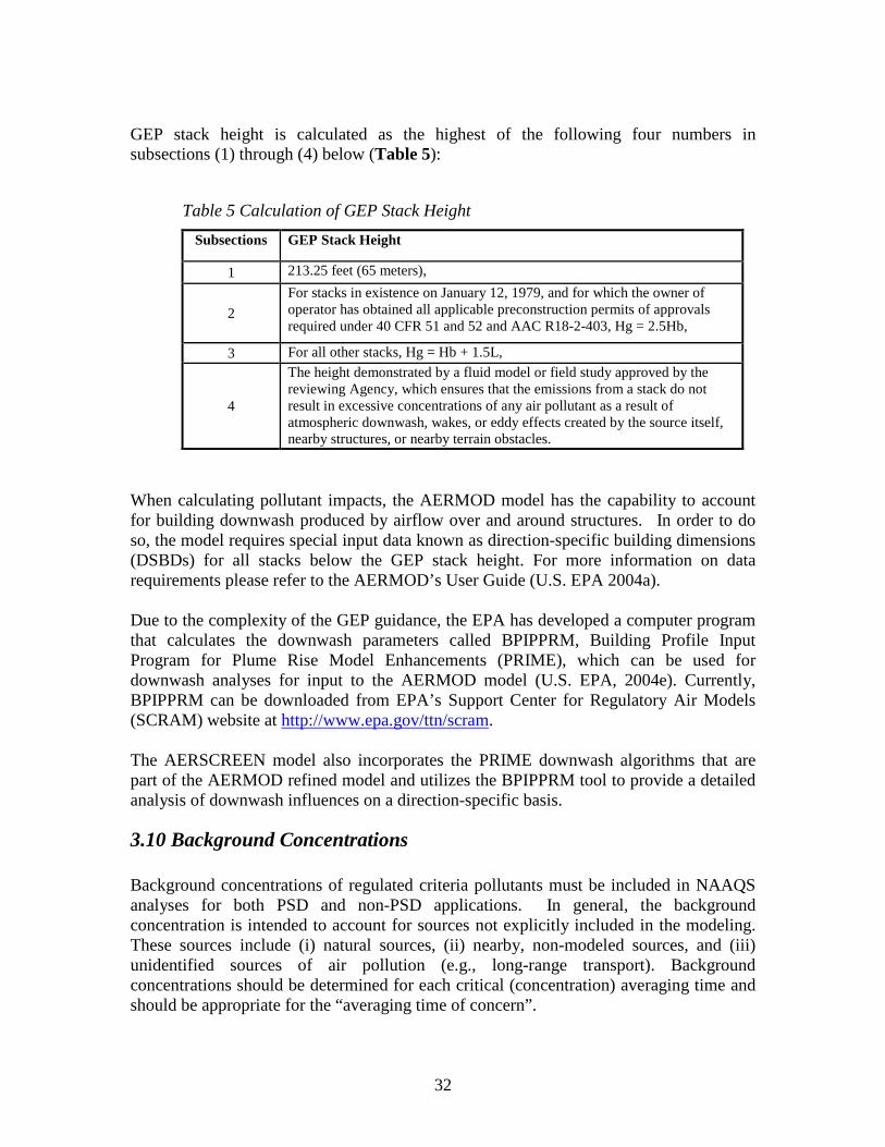
GEP stack height is calculated as the highest of the following four numbers in subsections (1) through (4) below (Table 5):

Table 5 Calculation of GEP Stack Height Subsections GEP Stack Height

1 213.25 feet (65 meters),

2 For stacks in existence on January 12, 1979, and for which the owner of operator has obtained all applicable preconstruction permits of approvals required under 40 CFR 51 and 52 and AAC R18-2-403, Hg = 2.5Hb,

3 For all other stacks, Hg = Hb + 1.5L,

4

The height demonstrated by a fluid model or field study approved by the reviewing Agency, which ensures that the emissions from a stack do not result in excessive concentrations of any air pollutant as a result of atmospheric downwash, wakes, or eddy effects created by the source itself, nearby structures, or nearby terrain obstacles.

When calculating pollutant impacts, the AERMOD model has the capability to account for building downwash produced by airflow over and around structures. In order to do so, the model requires special input data known as direction-specific building dimensions (DSBDs) for all stacks below the GEP stack height. For more information on data requirements please refer to the AERMOD’s User Guide (U.S. EPA 2004a). Due to the complexity of the GEP guidance, the EPA has developed a computer program that calculates the downwash parameters called BPIPPRM, Building Profile Input Program for Plume Rise Model Enhancements (PRIME), which can be used for downwash analyses for input to the AERMOD model (U.S. EPA, 2004e). Currently, BPIPPRM can be downloaded from EPA’s Support Center for Regulatory Air Models (SCRAM) website at http://www.epa.gov/ttn/scram. The AERSCREEN model also incorporates the PRIME downwash algorithms that are part of the AERMOD refined model and utilizes the BPIPPRM tool to provide a detailed analysis of downwash influences on a direction-specific basis.

3.10 Background Concentrations Background concentrations of regulated criteria pollutants must be included in NAAQS analyses for both PSD and non-PSD applications. In general, the background concentration is intended to account for sources not explicitly included in the modeling. These sources include (i) natural sources, (ii) nearby, non-modeled sources, and (iii) unidentified sources of air pollution (e.g., long-range transport). Background concentrations should be determined for each critical (concentration) averaging time and should be appropriate for the “averaging time of concern”.

32

Background concentrations should be representative of regional air quality in the vicinity of a facility. In determining whether the existing air quality data are representative, EPA suggests that Permittees consider three factors: (i) monitor location; (ii) data quality; and (iii) currentness (U.S. EPA, 1987b). Although this guidance is principally used for PSD sources, ADEQ believes this guidance is also helpful in assessing the representativeness of background concentrations for non-PSD sources as well. Typically, background concentrations should be determined based on the air quality data collected in the vicinity of the proposed project site. If a “regional” monitor is used to determine background, a discussion should be provided to compare the topography, climatology, and emissions sources between the area of the proposed project and the area where the “regional” monitor is located. On a case-by-case basis, ADEQ may allow the Permittee to use a data set obtained from other states if the data set is believed to be more representative. Note that some monitors are only running for a particular season (usually ozone season). Sufficient justification and documentation must be provided if a seasonal monitor is used for the background determination. If representative air quality data are unavailable, the Permittee may use some conservative air quality data for the background determination. The Permittee should explain why the utilization of these air quality data would provide a conservative estimate of the background concentration. If the Permittee proposes determining background concentration by modeling background sources, please consult with ADEQ. In Arizona, ambient monitoring is conducted by a number of governmental agencies and regulated industries. Each year, ADEQ compiles an annual monitoring report that summarizes monitored values from around Arizona. The reports also list active monitoring networks for various criteria pollutants. Electronic copies of the AQD’s annual air quality reports (required by A.R.S. §49-424.10) can be downloaded from ADEQ’s website at: http://www.azdeq.gov/function/forms/reports.html.

Currently, air quality annual reports containing monitoring data for the years 2000-2008 are available online. The most recent air monitoring data for Arizona can be obtained at the following website address: http://www.epa.gov/airdata/.

ADEQ suggests that Permittees select the background concentrations as described in Table 6. The most recent 3 years of ambient monitoring data should be used for background concentrations in NAAQS modeling analyses. Background concentrations should be representative of regional air quality in the vicinity of a facility. For more information, please refer to the Guideline on Air Quality Models.

33

Table 6 Determination of Background Concentrations NAAQS Pollutant

Averaging Time NAAQS Level NAAQS Form Background Form

Carbon Monoxide

8-Hour 9 ppm Not to be exceeded more than once per year

Highest concentration during most recent 3 years 1-Hour 35 ppm

Lead Rolling 3

Month Average

0.15 μg/m3 Not to be exceeded Highest concentration during most recent 3 years

Nitrogen Dioxide (NO2)

1-Houra 100 ppb

98th percentile of the annual distribution of the 1-hour daily maximum concentrations, averaged over 3 years

98th percentile of the annual distribution of daily maximum 1-hours values averaged across the most recent three years

Annual 53 ppb Annual Mean Highest annual concentration for most recent 3 years

Ozone 8-Hour 0.075 ppm

Annual fourth-highest daily maximum 8-hr concentration, averaged over 3 years

Not Applicable

PM2.5

Annual (primary) 12 μg/m3 Annual mean, averaged

over 3 years Average of the annual values over most recent 3 years

Annual (secondary) 15 μg/m3 Annual mean, averaged

over 3 years Average of the annual values over most recent 3 years

24-Hourb,c 35 μg/m3 98th percentile, averaged over 3 years

Average of the 98th percentile 24-hour values over most recent 3 years

PM10 24-Hourb 150 μg/m3 Not to be exceeded more than once per year on average over 3 years

Average of the highest yearly values for most recent 3 years

Sulfur Dioxide (SO2)

1-Houra 75 ppb

99th percentile of the annual distribution of the 1-hour daily maximum concentrations, averaged over 3 years

99th percentile of the annual distribution of daily maximum 1-hours values averaged across the most recent three years

3-hour 0.5 ppm Not to be exceeded more than once per year

Highest concentration during most recent 3 years

a Monthly/Seasonal/Annual hour-of-day monitored background concentrations may be used in some refined analyses. See Sections 7.1.4 and 7.2.3 for details. b Seasonal background concentrations may be used in some refined analyses. See Section 7.3.5 for details. c Monitored concentrations on a day-by-day basis may be used in some refined analyses. See Section 7.4.1 for details. Additionally, ADEQ occasionally requires that Permittees monitor one year of background data for particular criteria pollutants from a representative on-site location for PSD modeling analyses. At the earliest stages of the air quality permitting process, it is important that the Permittee communicate with ADEQ so that it can be determined whether or not background monitoring will be necessary. If background monitoring is necessary, the monitoring should follow monitoring guidance and QA/QC guidance from EPA. ADEQ relies upon the monitoring guidance provided in the Ambient Monitoring Guidelines for Prevention of Significant Deterioration (PSD) (U.S. EPA, 1987b). ADEQ also relies upon the QA/QC guidance provided in EPA’s Quality Assurance Handbook for Air Pollution Measurement Systems (five volume set).

34

3.11 Modeled Design Concentrations In a compliance demonstration, the applicable modeled design concentration must be calculated. Table 7 provides the summary of modeled design concentrations for individual criteria pollutants. It is worth mentioning that EPA has changed its recommendations on calculating modeled design concentration for 24-hour PM2.5. The March 23, 2010, clarification memo (U.S. EPA, 2010c) recommended that the modeled design concentration should be based on the highest average of the modeled 24-hour averages across 5 years for representative NWS data or the highest modeled average for one year (or multi-year average of 2 up to 5 complete years) of site-specific meteorological data. In the recent draft PM2.5 modeling guidance (U.S. EPA, 2013b), however, it was recommended to use the multi-year average of the 98th-percentile of 24-hour values instead of the highest average.

35

Table 7 Modeled Design Concentrations NAAQS Pollutant

Averaging Time Modeled Design Concentration Reference

Carbon Monoxide

8-Hour Highest, second highest concentrations over the entire receptor network for each year modeled a

40 CFR Appendix W 7.2.1 (U.S. EPA, 2005)

1-Hour Highest, second highest concentrations over the entire receptor network for each year modeled a

40 CFR Appendix W 7.2.1 (U.S. EPA, 2005)

Lead Rolling 3

Month Average

Highest modeled concentration over the entire receptor network regardless of one year or multiple years of meteorological data are used

40 CFR Appendix W 7.2.1 (U.S. EPA, 2005)

Nitrogen Dioxide (NO2)

1-Hour

- Highest of multi-year averages of the 98th percentile of the annual distribution of maximum daily 1-hour concentrations predicted each year at each receptor, if multiple years of meteorological data are used; - Highest of the 98th percentile of the annual distribution of maximum daily 1-hour concentrations predicted at each receptor if one year of meteorological data are used

Tyler Fox Memorandum dated June 28, 2010 (U.S. EPA, 2010a) and Tyler Fox Memorandum dated March 1, 2011 (U.S. EPA, 2011d)

Annual

Highest modeled concentration over the entire receptor network regardless of one year or multiple years of meteorological data are used

40 CFR Appendix W 7.2.1 (U.S. EPA, 2005)

PM2.5

Annual

- Highest of multi-year averages of annual concentrations at each receptor if multiple years of meteorological data are used - Highest annual concentration over the entire receptor network if one year of meteorological data is used

Stephen Page Memorandum dated March 4, 2013 (U.S. EPA, 2013b)

24-Hour

- Highest of multi-year averages of the 98th percentile of the annual distribution of 24-hour concentrations predicted each year at each receptor, if multiple year meteorological data are used; - Highest of the 98th percentile of the annual distribution of 24-hour concentrations predicted at each receptor if one year of meteorological data are used

Stephen Page Memorandum dated March 4, 2013 (U.S. EPA, 2013b)

PM10 24-Hour

The design concentration is dependent on the number of meteorological data years used in the analysis. In general, the (n+1)th highest concentration over the n-year period is the design value. For example, if five years of meteorological data are used, then the design concentration would be highest, sixth highest 24-hour modeled concentration that occurred at each receptor over that five-year period.

40 CFR Appendix W 7.2.1(U.S. EPA, 2005)

Sulfur Dioxide (SO2)

1-Hour

- Highest of multi-year averages of the 99th percentile of the annual distribution of maximum daily 1-hour concentrations predicted each year at each receptor, if multi-year meteorological data are used; - Highest of the 99th percentile of the annual distribution of maximum daily 1-hour concentrations predicted at each receptor if one year meteorological data is used

Tyler Fox Memorandum dated August 23, 2010. (U.S. EPA, 2010b)

3-hour Highest, second highest concentrations over the entire receptor network for each year modeled a

40 CFR Appendix W 7.2.1(U.S. EPA, 2005)

a If multi-year meteorological data are used, determine H2H for each year and then select the highest concentration as the modeled design concentration .

36

4 ADEQ PERMITTING JURISDICTION AND CLASSIFICATIONS

4.1 Air Quality Permitting Jurisdiction in Arizona Of Arizona’s 15 counties, three counties (Maricopa, Pinal, and Pima) (“local agency”, have obtained US EPA approval to regulate sources of air pollution within their county. ADEQ has jurisdiction in the other 12 counties. Unless the source falls under a category exclusively under ADEQ jurisdiction (regardless of location), such as (1) the smelting of metal ore, (2) petroleum refineries, (3) coal-fired electrical generating stations, (4) Portland cement plants, (5) other sources over which the State has asserted jurisdiction, these permitting authorities should be consulted directly for proposed projects that operate solely within their counties:

• Maricopa County (http://www.maricopa.gov/aq/) • Pima County (http://www.deq.pima.gov/air/index.html) • Pinal County (http://pinalcountyaz.gov/Departments/AirQuality/Pages/Home.aspx

Figure 2 provides map of counties, major highways, and selected towns and cities in Arizona. Portable sources are permitted by ADEQ for operations in Arizona that do not solely operate within Maricopa, Pinal, or Pima counties during the permit term. Portable sources that solely operate within Maricopa, Pinal, or Pima County should obtain an air quality permit from the local agency. Most Native American Reservations are under the jurisdiction of the federal Environmental Protection Agency. Some tribes in Arizona have US EPA approved air pollution control programs. More information regarding tribal programs can be found at:

• EPA Region 9 Tribal Air Programs in the Pacific Southwest (http://www.epa.gov/region9/air/tribal/index.html)

• Gila River Indian Community (http://www.gric.nsn.us/) • Fort McDowell Yavapai Nation (http://www.ftmcdowell.org/) • Navajo Nation (http://www.navajo.org/) • Salt River Pima-Maricopa Indian Community

(http://www.saltriver.pima-maricopa.nsn.us/) Additional information regarding many of Arizona’s tribes is available through the Intertribal Council of Arizona (http://www.itcaonline.com/). Figure 3 displays the locations of tribal lands located in Arizona.

37

4.2 Modeling Requirements for Permits and Registration

4.2.1 Classes of Permits and Registration There are different types of air quality permits that may need to address modeling:

• Class I permits - Class I permits are issued to any major source that meets the requirements of Arizona Administrative Code (A.A.C.) Title 18, Chapter 2, Article 302(B)(1). If a new source is a major stationary source, or a modification to an existing major source is a major modification as defined in A.A.C Title 18, Chapter 2, Article 401, these Class I permits or permit revisions are specifically referred to as a Prevention of Significant Deterioration (PSD) permit (the source is located in an attainment area) and non-attainment area New Source Review (NNSR) permit (the source is located in a non-attainment area).

• Class II permits - Class II permits are issued to sources that do not qualify for

Class I permits and that meet the requirements of A.A.C. Title 18, Chapter 2, Article 302(B)(2).

The PSD permits and NNSR permits/permit revisions are regulated under the major NSR program. The minor NSR program addresses both major and minor sources that undergo construction and modification activities that do not qualify as major, and it applies regardless of the designation of the area in which a source is located. The minor NSR program also fills a gap to address the minor NSR pollutants that do not trigger a PSD/NNSR review in a PSD/NNSR permit. The State of Arizona Minor NSR program (R18-2-334 of the A.A.C.) will be effective on December 2, 2015. The minor NSR program provides an opportunity to the Permittee to address minor NSR requirements by conducting a NAAQS modeling exercise or a Reasonable Available Control Technology (RACT) analysis. Notwithstanding the Permittee’s election to conduct a RACT analysis, the Director may request the Permittee conduct a NAAQS modeling analysis if a source or a minor NSR modification could interfere with attainment and maintenance of NAAQS based on the Director’s discretion. For minor NSR applicability and associated permit guidance please refer to ADEQ’s MINOR NSR GUIDANCE DOCUMENT (link). Besides Class I or II permits as discussed above, registrations are issued to sources that do not qualify for Class I or II permits and that meet the requirements of A.A.C. Title 18, Chapter 2, Article 302(B)(4). The State of Arizona registration program (R18-2-302.01 of the A.A.C.) will be effective on December 2, 2015. For registration applicability and associated registration guidance, please refer to ADEQ’s REGISTRATION GUIDANCE DOCUMENT.

4.2.2 Modeling Requirements

38

The modeling requirements for ADEQ permits and registration are pollutant specific, i.e., these must be evaluated pollutant by pollutant.

• Registration as defined in R18-2-302.01 of the A.A.C.

o Based on the Director’s discretion, ADEQ may perform modeling for criteria pollutants of concern on a case-by-case basis. ADEQ’s modeling exercise will be limited to a screening analysis. If the screening analysis indicates that the source could interfere with the attainment or maintenance of the NAAQS, the source will not be qualify for a registration and the Permittee should obtain a permit under R18-2-302 of the A.A.C.

• Minor NSR as defined in R18-2-334 of the A.A.C. (New Class II Permit or new Class I Permit that is not subject to the major NSR program, or minor NSR modification to a Class I or Class II source)

o The minor NSR review is triggered if a source will have the potential to

emit (PTE) for that pollutant at an amount equal to or greater than the permitting exemption threshold, or (ii) a modification that will increase the source’s PTE for that pollutant by an amount equal to or greater than the permitting exemption threshold. The permitting exemption thresholds for minor NSR pollutants are listed in Table 8.

Table 8 Permitting Exemption Thresholds

Pollutant Permitting Exemption Thresholds (tons per year)

PM10 7.5

PM2.5 Primary 5

Precursors (NOx/SO2) 20 SO2 20 NOx 20 VOC 20 CO 50

Lead 0.3 Precursors for ozone (VOC /NOx) 20

o Modeling is required for each criteria pollutant that triggers the minor NSR review if the Permittees is not implementing a RACT analysis for such pollutant.

o Notwithstanding the Permittee’s election to conduct a RACT analysis for minor NSR pollutants, modeling may be required for such pollutants if the source or modification could interfere with attainment or maintenance of the NAAQS based on the Director’s discretion.

39

o The Permittee may request ADEQ perform a screening modeling analysis. If doing so, the Permittee should provide ADEQ detailed facility layout, emissions and stack release parameters as discussed in Appendix A. If the screening analysis indicates possible interference with the attainment and maintenance of NAAQS, ADEQ will inform the Permittee to conduct a refined modeling analysis.

o If minor NSR review is applicable for ozone, the modeling requirements

for ozone are determined on a case-by-case basis due to the lack of screening tools and techniques for ozone modeling. The EPA is proposing to establish Model Emissions Rates for Precursors (MERPs) for ozone and the MERP values will likely be higher than the significant emission rates (40 tpy) (U.S. EPA., 2015). Therefore, an air quality assessment for ozone is not required if the PTE or the PTE increase for precursors are less than 40 tpy.

o If the PTE or PTE increase for NOx/SO2 is equal to or greater than 20 tpy,

ADEQ will adopt an interpollutant “offset ratios” method to address the secondary formation of PM2.5 under the minor NSR program. For details, please see Section 7.3.8.

o For detained modeling requirements, please refer to Section 5

“MODELING REQUIREMENTS UNDER MINOR NSR and REGISTRATION PROGRAM”.

• PSD as defined in R18-2-401 of the A.A.C.

o The Permittee should perform NAAQS modeling as well as PSD

increment modeling for criteria pollutants that trigger the PSD review. In addition, the Permittee should perform air quality related values (AQRVs) modeling if needed. For detained modeling requirements, please refer to Section 6 “MODELING REQUIREMENTS for PSD Sources”.

o Modeling is required for each criteria pollutant that triggers the minor

NSR review if the Permittees is not implementing a RACT analysis for such pollutant. The same requirements under the minor NSR program as discussed above should apply.

40

Figure 2 Map of Arizona

SANTA CRUZ

GREENLEE

SANTA CRUZ

41

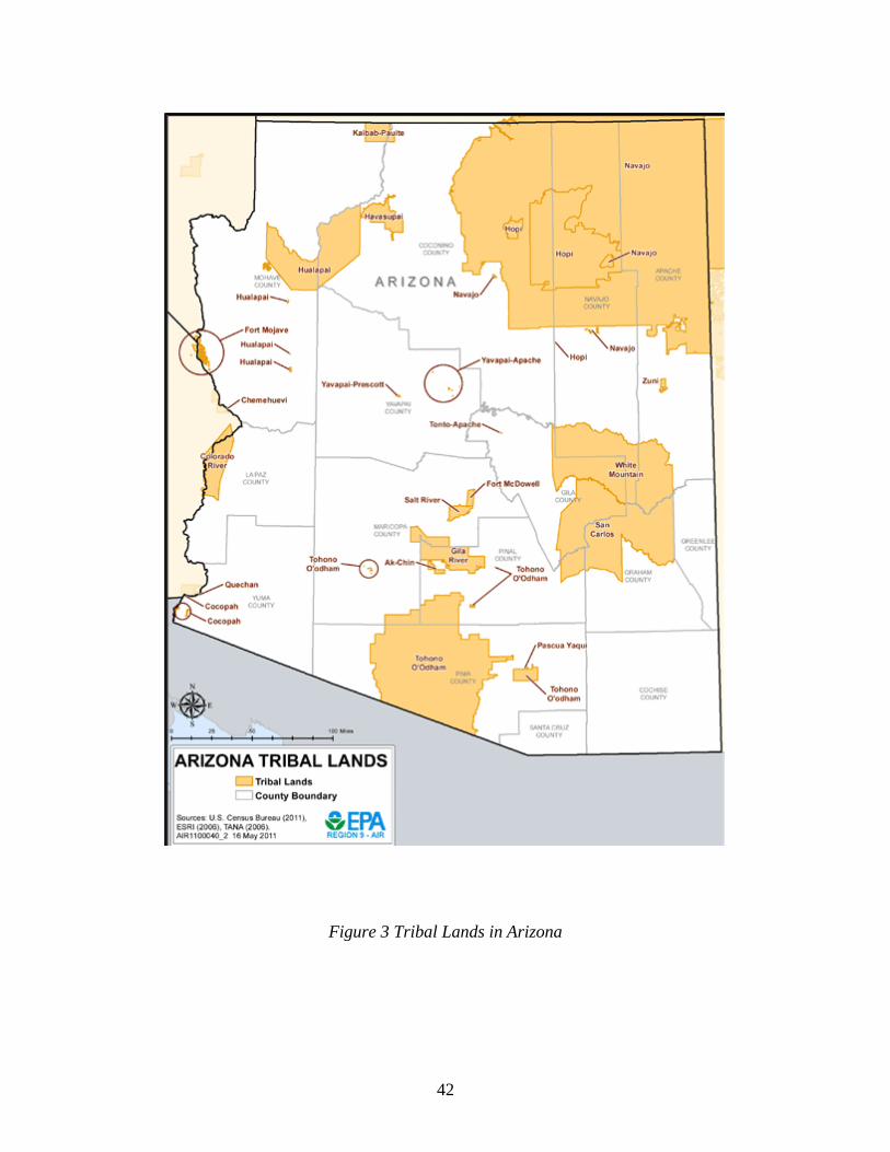
Figure 3 Tribal Lands in Arizona

42

5 MODELING REQUIREMENTS UNDER MINOR NSR and REGISTRATION PROGRAM This section applies to:

• New Class I source that is not subject to PSD/NNSR review ; • Minor NSR pollutants that trigger the minor NSR review in a PSD/NNSR source; • New Class II source; • Minor NSR modification to a Class I or Class II source; • Registration source of concern.

The modeling analysis should demonstrate that emissions from the new source or modification will not interfere with attainment or maintenance of the NAAQS. In particular, the modeling analysis should demonstrate either of the following:

• The emissions from the source or minor modification will have an ambient impact below the significant levels (SILs) as defined in R18-2-401 of the A.C.C.;

• The ambient concentrations resulting from the source or modification combined with representative background concentrations of minor NSR pollutants will not cause the violation of the NAAQS or not further exacerbate the non-attainment status.

5.1 Modeling Demonstration for Attainment Pollutants

For a new Class I or Class II source, the impacts from all sources within the facility should be assessed for criteria pollutants that trigger the minor NSR review. The maximum potential short-term and long-term emission rates based on PTE should be modeled. If the modeling results are below SILs, the modeling demonstration is satisfied. Otherwise, the modeling results are added to representative ambient background concentrations and the total concentrations are then compared to the NAAQS. For a modification to a Class I or Class II source, the PTE increase associated with the proposed project may be modeled to compare with the SILs. If the modeling results are below the SILs, the modeling demonstration is satisfied. Otherwise, the post-project facility-wide emissions should be modeled, and the modeling results are then added to representative ambient background concentrations to compare with the NAAQS. The procedures above also apply to a registration source. However, for a registration source, the emissions taking into account any elective limits or controls should be modeled. Elective limits or control are defined in R18-2-302.01.F of the A.A.C.

43

Unlike the methods used in NAAQS analyses for PSD permit applications, inclusion of regional sources under the minor NSR program or registration program is typically not required. However, on a case-by-case basis, ADEQ reserves the right to request modeling which includes the minor NSR /registration source in question and additional nearby or regional sources. If the model indicates that a NAAQS is initially exceeded, it is the responsibility of the Permittee to consider several options to prevent the NAAQS exceedance. Preliminary NAAQS exceedances might be avoided by:

• Refining emissions estimates by using other defensible emission factors than those used in the preliminary modeling analysis;

• Limiting operational hours or process throughputs; • Optimizing stack parameters for better pollutant dispersion (i.e. raise stack

heights, increase exhaust airflows (subject to restrictions on prohibited dispersion techniques), or crown stack diameters to obtain higher exhaust velocities);

• Relocating sources to other portions of a facility which would lead to lower modeled impacts;

• Source testing to refine emissions estimates; • Installing pollution controls to limit emissions

Note that the EPA’s “prohibited dispersion techniques” as defined in 40 CFR 51.100 (hh)(1)(i)-(iii) should not be used. For registration, the controls should be limited to elective control as defined in R18-2-302.01.F of the A.A.C.

5.2. Modeling Demonstration for Nonattainment Pollutants If the source is located in a nonattainment area for any criteria pollutants (nonattainment pollutants), the Permittee should demonstrate that the emissions from the source or modification will have an ambient impact below the significant levels (SILs) or will not further exacerbate the nonattainment status. Due to the complexities in modeling demonstration for nonattainment pollutants, the Permittee may explore the following options on a case-by-case basis:

• New Source

o SILs Comparison: The Permittee may model the facility-wide emissions to demonstrate that the source will have an ambient impact below the SILs. If the ambient impacts from the source are greater than SILs based on a preliminary modeling analysis, the Permittee may evaluate additional controls or dispersion techniques to mitigate the source’s impact to be below the SILs. The recommended additional controls or dispersion techniques are the same to those for preventing NAAQS exceedances as discussed in Section 5.1.

44

o NAAQS Comparison: For some circumstances, although the facility is

located in a nonattainment area, the most recent three years of ambient monitoring data may indicate that the background concentrations for the project site area are below the NAAQS. For this case, the Permittee may model the facility-wide emissions and add modeling results to representative ambient background concentrations to demonstrate that the total concentrations are below the NAAQS.

• Modification

o SILs Comparison: The Permittee may model the emissions increase

associated with the proposed project to demonstrate that the proposed project will have an ambient impact below the SILs. If the ambient impacts from the project are greater than SILs based on a preliminary modeling analysis, the Permittee may evaluate additional controls or dispersion techniques to mitigate the project’s impact to be below the SILs. The recommended additional controls or dispersion techniques are the same to those for preventing NAAQS exceedances as discussed in Section 5.1.

o NAAQS Comparison: For some circumstances, although the facility is

located in a nonattainment area, the most recent three years of ambient monitoring data may indicate that the background concentrations for the project site area are below the NAAQS. For this case, the Permittee may model the post-project facility-wide emissions and add modeling results to representative ambient background concentrations to demonstrate that the total concentrations are below the NAAQS.

o Pre-Project and Post-Project Comparison: Not limiting to the project itself, this option allows Permittee to reduce the ambient impacts from the facility by exploring control/dispersion options for other sources within the facility that are not affected by the project. The Permittee may model the pre-project and post-project facility-wide emissions separately to demonstrate that the post-project ambient impacts are equal to or less than the pre-project ambient impacts.

6 MODELING REQUIREMENTS FOR PSD SOURCES The following section reviews ADEQ’s requirements for sources that are subject to PSD regulations. The PSD regulation is targeted for individual pollutants. If any of the pollutants emitted by a source is above the threshold level for PSD, the source is subject

45

to PSD for that pollutant. Those pollutants that are below the threshold level are not subject to PSD.

6.1 NAAQS Analyses for Pollutants That Do Not Trigger PSD For pollutants that trigger the minor NSR review, please refer to Section 5 for modeling requirements. For pollutants that do not trigger the minor NSR review, modeling is generally not required.

6.2 Overview of PSD Modeling Procedures For PSD triggering pollutants, ADEQ requires that Permittee follow EPA’s New Source Review Workshop Manual (U.S. EPA, 1990) and other applicable PSD guidance set forth in the EPA’s Guideline on Air Quality Models to complete the air quality impact analysis. The Draft New Source Review Workshop Manual (see Chapters C, D, and E) provides a good overview and examples of modeling analyses required for sources that trigger PSD. http://www.epa.gov/ttn/nsr/gen/wkshpman.pdf The PSD modeling analysis is performed in two steps: a preliminary analysis (often referred to as a significant impact analysis), and if required, a full impact analysis. The preliminary analysis estimates ambient concentrations resulting from the proposed project for pollutants that trigger PSD requirements. For this analysis, a loads analysis should be performed to determine that project impacts are not underestimated. The results of the preliminary analysis determine whether Permittee must perform a full impact analysis for a particular pollutant. If the ambient impacts from the preliminary analysis are greater than the PSD Significant Impact Levels (SILs, see Table 9), then the extent of the Significant Impact Area (SIA) of the proposed project is determined. Initially, the SIA is determined for every relevant averaging time for a particular pollutant. The final SIA for that pollutant is the largest area for each of the various averaging times. The preliminary, facility-only impact analysis involves modeling impacts for comparison to both the PSD Class II Significant Impact Levels and Significant Monitoring Concentration (SMC) Levels as shown in Table 9. If the facility-only impacts exceed the SMC levels, then pre-application air quality monitoring may be required. Note that on January 22, 2013, the U.S. Court of Appeals for the District of Columbia vacated parts of the PSD rules establishing the SMC for PM2.5, thereby precluding the use of the SMC as a “de minimis” level to avoid pre-construction monitoring for PM2.5. Due to the nature of this court decision, there may be legal bearing on the use of SMCs for pollutants other than PM2.5. In a brief summary of the court decision issued on January 29, 2013, EPA states that “given the court’s broadly stated holding that SMCs are not permissible, the EPA is also assessing the decision’s impact on SMCs for other pollutants”. The outcome of EPA’s assessment is still pending and therefore the full impact of the court decision on the use of SMCs to avoid pre-construction monitoring for other pollutants is uncertain at this time. Until the federal rules implementing the SMCs are legally revised, ADEQ

46

recommends continued use of the SMCs for all pollutants except for PM2.5. Alternatively, sources may avoid the implications of the court ruling by demonstrating that adequate, representative monitoring data to establish background conditions for the facility are available.

Table 8 PSD Increments, Significant Emission Rates, Modeling Significance Levels, and Monitoring De Minimis Concentrations

Pollutant Averaging Period

PSD Significant

Emission Rates (tons/year)

PSD Increment (µg/m3)

Significant Impact Level

(µg/m3)

Monitoring De Minimis

Concentrations (µg/m3) Class

I Class

II Class

III Class

I Class

II PM10 24-hour 15 8 30 60 0.3 5 10

PM2.5 24-hour 10 (40a) 2 9 18 0.07b 1.2b Annual 1 4 8 0.06b 0.3b

NO2 1-hour 40 of NOx 7.5c Annual 2.5 25 50 0.1 1 14

SO2 1-hour 40 7.8d 3-hour 25 512 700 1 25

CO 1-hour 100 2,000 8-hour 500 575

Ozone 8-hour 40 of VOC VOC emissions increase > 100 tpy

Lead Rolling 3

month average

0.6 0.1

a SO2, NOx, and VOCs as precursors b SILs may be used under some circumstances (see Section 7.3) c Interim 1-hour SIL, 4 ppb d Interim 1-hour SIL, 3 ppb The full impact analysis expands the preliminary impact analysis by considering emissions from both the proposed project as well as other sources in the SIA. The full impact analysis may also consider other sources outside the SIA that could cause significant impacts in the SIA of the proposed source. The results from the full impact analysis are used to demonstrate compliance with NAAQS and PSD increments. The source inventory for the cumulative NAAQS analysis includes all nearby sources that have significant impacts within the proposed source SIA, while the source inventory for the cumulative PSD increment analysis is limited to increment-affecting sources (new sources and changes to existing sources that have occurred since the applicable increment baseline date).

The full impact analysis is limited to receptor locations within the proposed project's SIA. The modeling results from the NAAQS cumulative impact analysis are added to representative ambient background concentrations and the total concentrations are compared to the NAAQS. Conversely, the modeled air quality impacts for all

47

increment-consuming sources are directly compared to the PSD increments to determine compliance (without consideration of ambient background concentrations).

6.2.1 NAAQS Modeling Inventory In addition to modeling the proposed source and adding background values, EPA requires that, at a minimum, all nearby sources be explicitly modeled as part of the full NAAQS analysis for PSD. The Guideline on Air Quality Models defines a nearby source as any point source expected to cause a significant concentration gradient in the vicinity of the proposed new source or modification. For PSD purposes, vicinity is defined as the significant impact area (SIA) for each pollutant. However, the location of such nearby sources could be anywhere within the significant impact area or an annular area extending 50 kilometers beyond the SIA. For the full NAAQS modeling analyses, all permitted sources within the SIA must be explicitly modeled. In addition, all permitted sources located outside the SIA and within the annular area extending 50 km from the SIA must also be included if they have a potential to affect air quality near the proposed source, as described in Chapter C, Section IV.C.1 of the Draft New Source Review Workshop Manual (U.S. EPA, 1990). The inclusion of a regional source can be determined by using the ‘20D’ approach (also followed by Ohio EPA), also known as the North Carolina Protocol. The “20D” approach assumes a linear inverse proportional relationship between source emissions and impacts with distance. A “20D” facility-level screening approach is used to eliminate a majority of regional facilities from the PSD NAAQS modeling analysis that would not be expected to have a significant impact on analysis results. Under this approach, the Permittee may exclude sources that have potential allowable emissions (Q) in tons/yr that are less than 20 times the distance (“20D”) between the two sources in kilometers. Those sources that are not eliminated using the “20D” approach should be modeled in the full NAAQS analysis. Cumulative impact assessments based on the procedures above will generally be acceptable as the basis for permitting decisions. However, in the recent 1-hour NO2 modeling guidance (U.S.EPA, 2011d) and draft PM2.5 modeling guidance (U.S. EPA, 2013b), EPA cautions against the literal and uncritical application of very prescriptive procedures for identifying which nearby sources should be included in the modeled emission inventory for NAAQS compliance demonstrations, such as described in the draft New Source Review Workshop Manual. EPA suggests that the emphasis on determining which nearby sources to include in the cumulative modeling analysis should focus on the area within about 10 kilometers of the project location in most cases. However, several application-specific factors should be considered when determining the appropriate inventory of nearby sources to include in the cumulative modeling analysis, including the potential influence of terrain characteristics on concentration gradients, and the availability and adequacy of ambient monitoring data to account for background sources. Sufficient justification must be provided if the Permittee proposes using a 10 km radius of background sources in the modeled emission inventory.

48

The ADEQ State Implementation Plan (SIP) Section provides regional source emission inventories to Permittee. The appropriate contact in the SIP Section can be reached at 602-771-7665.

6.2.2 Increment Modeling Inventory A PSD increment is the maximum allowable increase in concentration that is allowed to occur above a baseline concentration for a pollutant. The baseline concentration is defined for each pollutant (and relevant averaging time) and, in general, is the ambient concentration existing at the time that the first complete PSD permit application affecting an area is submitted. Significant deterioration is said to occur when the amount of new pollution would exceed the applicable PSD increment. According to PSD Guidelines, the increment inventory to be considered in the modeling analysis includes all increment-affecting sources located within the SIA of the proposed new source or modification. In addition, all increment-affecting sources located within 50 kilometers of the SIA should also be included in the inventory if they, either individually or collectively, affect the amount of PSD increment consumed. In general, the stationary sources of concern for the increment inventory are those stationary sources with actual emissions changes occurring since the minor source baseline date. However, it should be noted that certain actual emissions changes occurring before the minor source baseline date (i.e. at major stationary point sources) also affect the increments. To clarify, the types of stationary point sources that should be initially reviewed to determine the need to include them in the increment inventory fall under two specific time frames:

After the major source baseline date:

• Existing major stationary sources having undergone a physical change or change in their method of operation

• New major stationary sources After the minor source baseline date:

• Existing stationary sources having undergone a physical change or change in their method of operation

• Existing stationary sources having increased hours of operation or capacity utilization (unless such change was considered representative of baseline operating conditions)

The Draft New Source Review Workshop Manual (U.S. EPA, 1990) provides details regarding the major source baseline date, trigger date, and minor source baseline dates. The major source baseline date and trigger dates are fixed. The major source baseline dates are shown in Table 10.

49

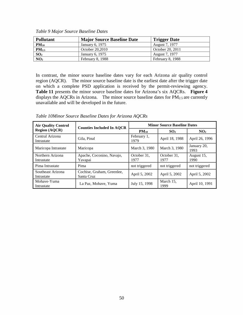
Table 9 Major Source Baseline Dates

Pollutant Major Source Baseline Date Trigger Date PM10 January 6, 1975 August 7, 1977 PM2.5 October 20,2010 October 20, 2011 SO2 January 6, 1975 August 7, 1977 NO2 February 8, 1988 February 8, 1988 In contrast, the minor source baseline dates vary for each Arizona air quality control region (AQCR). The minor source baseline date is the earliest date after the trigger date on which a complete PSD application is received by the permit-reviewing agency. Table 11 presents the minor source baseline dates for Arizona’s six AQCRs. Figure 4 displays the AQCRs in Arizona. The minor source baseline dates for PM2.5 are currently unavailable and will be developed in the future.

Table 10Minor Source Baseline Dates for Arizona AQCRs

Air Quality Control Region (AQCR) Counties Included In AQCR

Minor Source Baseline Dates PM10 SO2 NO2

Central Arizona Intrastate Gila, Pinal February 1,

1979 April 18, 1988 April 26, 1996

Maricopa Intrastate Maricopa March 3, 1980 March 3, 1980 January 20, 1993

Northern Arizona Intrastate

Apache, Coconino, Navajo, Yavapai

October 31, 1977

October 31, 1977

August 15, 1990

Pima Intrastate Pima not triggered not triggered not triggered Southeast Arizona Intrastate

Cochise, Graham, Greenlee, Santa Cruz April 5, 2002 April 5, 2002 April 5, 2002

Mohave-Yuma Intrastate La Paz, Mohave, Yuma July 15, 1998 March 15,

1999 April 10, 1991

50

Figure 4 Air Quality Control Regions in Arizona

6.2.3 Additional Impact Analyses PSD Permittee must prepare additional impact analyses for each PSD triggering pollutant. These additional analyses assess the impacts of air, ground, and water pollution on soils, vegetation, and visibility caused by any increase in emissions of any regulated pollutant from the source or modification under review, and from associated growth. Details regarding these analyses can be found in Chapter D of the Draft New Source Review Workshop Manual (U.S. EPA, 1990).

51

6.2.4 Class I Area Impact Analyses The Federal Land Manager’s Air Quality Related Values Work Group (FLAG) was formed to develop a more consistent approach for the Federal Land Managers (FLMs) to evaluate air pollution effects on their resources. Of particular importance are the New Source Review (NSR) program and the review of PSD air quality permit applications. FLAG’s goals are to provide consistent policies and processes for identifying air quality related values (AQRVs) and for evaluating the effect of air pollution on AQRVs, primarily those in Federal Class I air quality areas, but in some instances, in Class II areas. Federal Class I areas are defined in the Clean Air Act as national parks over 6,000 acres and wilderness areas and memorial parks over 5,000 acres that were established as of 1977. All other federally managed areas are designated as Class II. 40 CFR 51.307 requires the operator of any new major stationary source or major modification that may affect visibility in any Federal Class I area to contact the FLM for that area. It should be addressed that, there is no absolute distance cutoff for FLM notification because the Clean Air Act (CAA) does not establish any distance criteria with respect to the FLMs’ “affirmative responsibility” to protect AQRVs in Class I areas. EPA guidance states that permitting authorities should notify the FLM of all sources proposing to locate within 100 km of a Class I area, and of “very large sources” locating greater than 100 km if they have the potential to affect Class I areas (U.S. EPA, 1979). The FLAG guidance document recommends that Permittee conduct an analysis of the AQRV’s for Class I areas within 300 km of a source. However, the distance of 300 km is based on the modeling capabilities of CALPUFF rather than any laws or regulations. Class I increments have been established for PM10, PM2.5, SO2, and NO2 and are listed in Table 9. These represent the maximum increases in ambient pollutant concentrations allowed over baseline concentrations. The class I increment analysis should be conducted using the same modeling methodology as that used in the Class II area analysis and may incorporate the use of long range transport models such as CALPUFF. The FLAG guidance document (FLAG Phase 1 Report, 2010; FLAG, 2011) should be followed when conducting an AQRV impact analysis. For sources located or proposing to locate greater than 50 km from a Class I area, Permittee may choose to utilize the Q/D ≤ 10 initial screening criteria, in accordance with the FLAG 2010 guidance document, to determine whether further AQRV analysis is required. However, it should be noted that this screening approach is for AQRVs only (e.g. visibility) and is not applicable for Class I increment analyses. See the Federal Land Managers’ Air Quality Related Values Work Group (FLAG) for more information at: http://www2.nature.nps.gov/air/Permits/flag/index.cfm For long-range modeling with CALPUFF, the most recent and readily available Penn State/NCAR Mesoscale Model (MM5) or Weather Research and Forecasting (WRF) data should be used to generate metrological data files with grid spacing no less than 4 km to ensure proper wind field development. Regarding CALMET settings, please use EPA-FLM recommended CALMET input files values (U.S. EPA, 2009b). Mesoscale

52

Model Interface Program (MMIF), which converts prognostic meteorological model output fields to the parameters and formats required for direct input into dispersion models, should not be used for regulatory purposes unless EPA provides appropriate guidance and other support for such use.

During the PSD permitting process, the Permittee should work closely with the FLM to address any AQRV related concerns. Table 12 lists the name of each Class I area located in Arizona and the managing agency responsible for each. Figure 5 shows the locations of Class I areas in Arizona. Table 11 Class I Areas Located in Arizona

Class I Area Managing Agency

National Parks

Grand Canyon National Park Service

Petrified Forest National Park Service

National Wilderness Areas

Chiricahua National Monument National Park Service

Chiricahua Forest Service

Galiuro Forest Service

Mazatzal Forest Service

Mt. Baldy Forest Service

Pine Mountain Forest Service

Saguaro National Monument National Park Service

Sierra Ancha Forest Service

Superstition Forest Service

Sycamore Canyon Forest Service

53

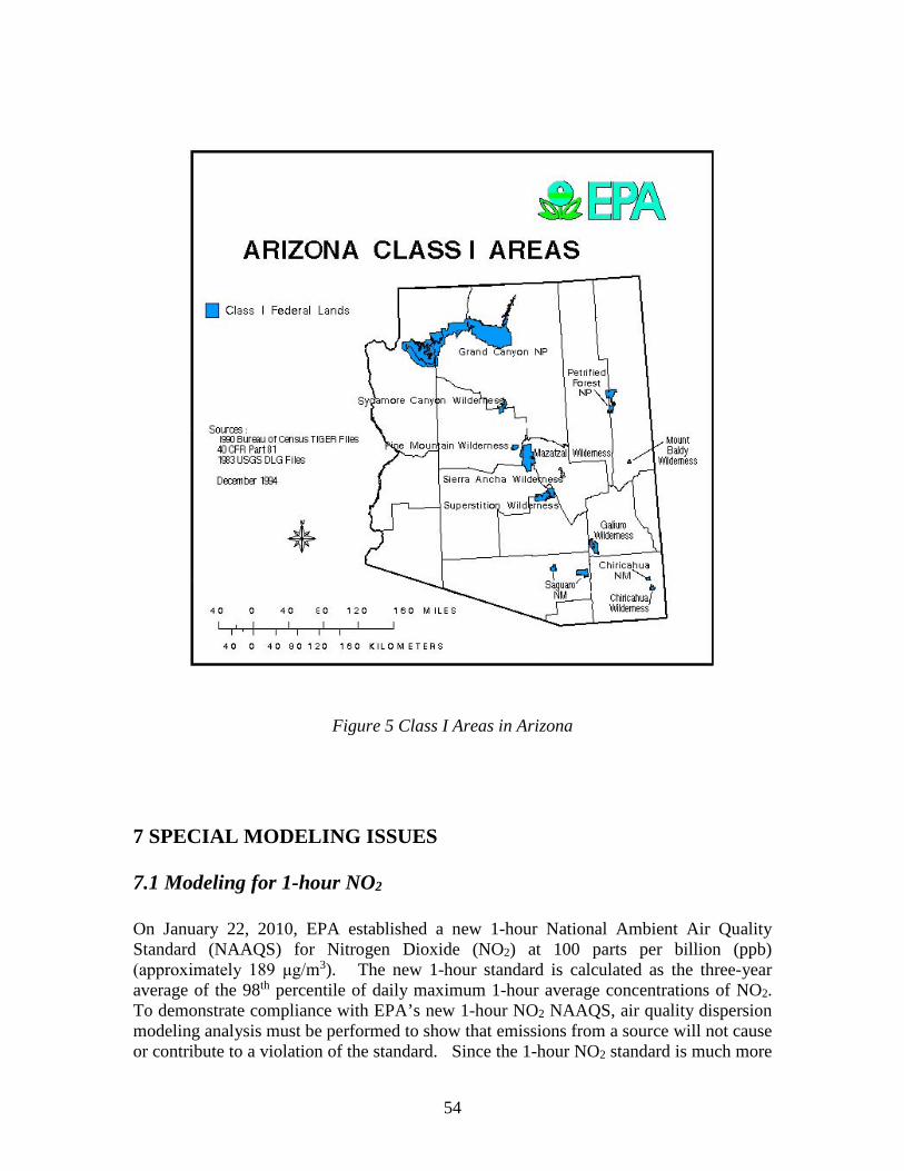
Figure 5 Class I Areas in Arizona

7 SPECIAL MODELING ISSUES

7.1 Modeling for 1-hour NO2 On January 22, 2010, EPA established a new 1-hour National Ambient Air Quality Standard (NAAQS) for Nitrogen Dioxide (NO2) at 100 parts per billion (ppb) (approximately 189 μg/m3). The new 1-hour standard is calculated as the three-year average of the 98th percentile of daily maximum 1-hour average concentrations of NO2. To demonstrate compliance with EPA’s new 1-hour NO2 NAAQS, air quality dispersion modeling analysis must be performed to show that emissions from a source will not cause or contribute to a violation of the standard. Since the 1-hour NO2 standard is much more

54

stringent than the previous NAAQS, it has been found that demonstrating compliance with the new standard is significantly challenging, particularly for short stacks and small facility footprints (AIWG, 2012). To assist sources and permitting authorities in carrying out the required air quality analysis for 1-hour NO2 compliance demonstrations, EPA has issued two guidance memorandums:

• Applicability of Appendix W Modeling Guidance for the 1-hour NO2 National Ambient Air Quality Standard (U.S. EPA, 2010a);

• Additional Clarification Regarding Application of Appendix W Modeling Guidance for the 1-hour NO2 National Ambient Air Quality Standard (U.S. EPA, 2011d).

While the two memorandums are specifically for major sources and major modifications that are subject to Prevention of Significant Deterioration (PSD) requirements, ADEQ believes that some principles and guidance can apply to minor sources, in part, to ensure consistency of treatment in permitting and to ensure that it is not imposing different requirements on minor sources than those to which PSD sources are subject. The following guidance describes ADEQ’s requirements and recommended procedures for 1-hour NO2 permit modeling. Due to the technical issues associated with 1-hour NO2 modeling, the guidance will be amended periodically to incorporate new modeling guidance developed by EPA.

7.1.1 Emission Rate For sources modeled to determine compliance with the 1-hour NO2 NAAQS, the maximum 1-hour emission rates must be used unless otherwise discussed or otherwise approved by ADEQ. For example, an emission rate lower than the maximum 1-hour rate may be used if it will be enforceable through a permit condition. For modeling some intermittent sources with an uncertain operating frequency, ADEQ may also allow using an annualized hourly emission rate rather than the maximum hourly emission rate (see Section 7.1.6).

7.1.2 Significant Impact Level The EPA’s interim significant impact level (SIL) (4 ppb, 7.5 μg/m3) for 1-hour NO2 should be used unless EPA promulgates an official 1-hour NO2 SIL. To determine whether a cumulative impact assessment is needed for PSD sources, the interim SIL should be compared to the highest of the 5-year average of the maximum modeled 1-hour NO2 concentrations predicted at each receptor (if multiyear meteorological data are used)

55

or the highest modeled 1-hour NO2 concentration (if one-year meteorological data are used).

7.1.3 Three-tiered Approach for 1-hour NO2 Modeling Based on the EPA’s memorandums dated June 28, 2010 and March 01, 2011, the following three-tiered approach is recommended for 1-hour NO2 modeling:

• Tier 1 Total Conversion - assuming full conversion of NO to NO2 without any additional justification.

• Tier 2 Ambient Ratio Method (ARM) - multiply Tier 1 result by empirically-derived NO2/NOx ratio, with 0.8 as default ambient ratio for the 1-hour NO2 standard without additional justification. Note that the national annual default for NO2/NOx ratio is 0.75.

• Tier 3 - Plume Volume Molar Ratio Method (PVMRM)/ Ozone Limiting Method (OLM) - the two approaches are available as non-regulatory-default options within the AERMOD model. Both of these options account for ambient conversion of NO to NO2 in the presence of ozone, namely the ozone titration mechanism. The main distinction between PVMRM and OLM is the approach taken to estimate the ambient concentration of NO and O3 for which the ozone titration mechanism should be applied. Since the EPA’s memorandums do not indicate any preference between the two options, it is the Permittee’s responsibility to justify which method is more suitable, if the Tier 3 approach is used.

Two key model inputs for both the PVMRM and OLM options, namely in-stack ratios of NO2/NOX emissions and background ozone concentrations, will be discussed in detail later. For OLM, the “OLMGROUP ALL” option should be used if multiple sources are modeled. Per EPA’s guidance, the ambient equilibrium ratio is 0.9 for both OLM and PVMRM.

7.1.4 Determining Background Concentrations Background Concentration for 1-hour NO2 In general, the guidance in Section 3.10 should be followed when determining background concentrations for 1-hour NO2. Since there are very limited NO2 monitoring sites in Arizona and nearly all monitoring sites are located in the Phoenix/Tucson metropolitan area, ADEQ may allow Permittee to use a data set obtained from other states if the data set is believed to be more representative. The Permittee should review and compare the topography, climatology, and emissions sources (such as vehicle emissions and industrial sources) between the area of the proposed project and

56

the area where the selected monitor is located. ADEQ is planning to operate a NO2 monitor in Alamo Lake, which will help estimate the background concentrations for some remote areas in future. The Permittee may use a uniform monitored background concentration or hour-of-day monitored background concentrations in the modeling compliance demonstration for the 1-hour NO2 NAAQS. Using a uniform monitored background concentration. The 98th percentile of the annual distribution of daily maximum 1-hour values averaged across the most recent three years of monitored data should be used for determining the background concentration for 1-hour NO2. Using hour-of-day monitored background concentrations. ADEQ recommends using the following three refined background datasets:

• 98th percentile of the Monthly Hour-Of-Day (1st Highest): For each of the three years under review, Monthly Hour-Of-Day is determined by organizing all of the NO2 concentrations by hour of day (1AM, 2AM, 3AM, etc) for each month in descending order and selecting the 1st highest NO2 concentrations for each hour of the day. The background concentrations are then determined as the 3 year average of the 1st highest concentrations for each hour of the day and month.

• 98th percentile of the Seasonal Hour-Of-Day (3rd Highest): For each of the three years under review, Seasonal Hour-Of-Day is determined by organizing all of the NO2 concentrations by hour of day (1AM, 2AM, 3AM, etc) for each season of the year in descending order and selecting the 3rd highest NO2 concentrations for each hour of the day. The background concentrations are then determined as the 3 year average of the 3rd highest concentrations for each hour of the day and season.

• 98th percentile of The Annual Hour-Of-Day (8th Highest): For each of the three

years under review, Annual Hour-of-Day is determined by organizing all of the NO2 concentrations by hour of day (1AM, 2AM, 3AM, etc) in descending order and selecting the 8th highest NO2 concentration for each hour of the day. The background concentrations are then determined as the 3 year average of the 8th highest concentrations for each hour of the day.

It should be noted that the approaches presented above are not an exhaustive list of approaches that are acceptable to ADEQ. Please consult with ADEQ if other refined methods are used.

Current on-line sources for 1-hour NO2 are listed as follows:

• EPA AirData: 1-hour values (first, second, 98th percentile); in most cases, monitoring occurs in high population areas

57

http://www.epa.gov/airdata/

• EPA Air Quality System (AQS) raw data: EPA provides hourly data sets in raw format that can be downloaded at http://www.epa.gov/ttn/airs/airsaqs/detaildata/downloadaqsdata.htm

Background Concentration for Ozone Background ambient ozone (O3) concentrations are required for the applications of the OLM and PVMRM options in AERMOD. Ozone concentrations can be entered into the model as a single (most conservative) value or hourly datasets. Using a single value. To be defensible, the highest hourly ozone concentration over the modeled period should be used. The default value of 40 ppb in AERMOD or annual average ozone concentrations should not be used. The highest hourly ozone concentrations are available at EPA AirData: http://www.epa.gov/airdata/ Using hourly data sets. Current on-line sources for 1-hour O3 are listed as follows:

• EPA Air Quality System (AQS) raw data: EPA provides hourly data sets in raw format that can be downloaded at http://www.epa.gov/ttn/airs/airsaqs/detaildata/downloadaqsdata.htm

• Clean Air Status and Trends Network (CASTNET): Hourly datasets are available

for three remote areas, including Chiricahua National Monument, Grand Canyon National Park, and Petrified National Park. http://epa.gov/castnet/javaweb/index.html

Gap filling for missing ozone. For a single missing hour, use linear interpolations to fill in the missing concentrations based on the previous and subsequent hour concentrations or simply use the higher one. For multiple missing hours, it is recommended to use the following approaches to fill in gaps:

• Use the highest hourly ozone concentration over the modeled period without any additional justifications;

• Determine the maximum hourly ozone concentration for each season and use the seasonally maximum concentration to substitute for any missing data within that season;

• Determine the maximum hourly ozone concentration for each month and use the monthly maximum concentration to substitute for any missing data within that month; and

• For each month, calculate the maximum ozone concentration for each diurnal hour and use these hourly maximum concentrations to fill in their corresponding missing diurnal hours.

58

It should be noted that the approaches presented above are not an exhaustive list of procedures that are acceptable to ADEQ. Please consult with ADEQ if other refined methods or procedures are used.

7.1.5 In-Stack NO2/NOX Ratio The NO2/NOx in-stack ratio is critical since it defines the portion of the model predicted NOx concentration that will be automatically converted to NO2. The remaining portion released into the air may or may not undergo conversion to NO2 prior to it reaching a receptor point. In the case of lower-level releases, the transport distance may be a few hundred meters or less. In this case, the predicted concentration would be in-stack ratio dependent with minimal NO2 formation due to reactions with O3. Hence, the user’s choice of an in-stack ratio could be the determining factor in model predictions. Prior to the new 1-hour NO2 NAAQS, a commonly used in-stack ratio for purposes of modeling the annual average NO2 impact was 0.10. Currently, limited information is available on in-stack NO2/NOx ratios for 1-hour NO2 nationwide. EPA has started collecting in-stack NO2/NOx data for varied source categories, if available. However, it is unclear how long it will take EPA to compile and develop appropriate in-stack ratios for specific sources. During the transition period, it is suggested to use the following hierarchy in-stack ratio data sources:

• Source testing data reviewed and verified by a local air district, state, and/or EPA (ADEQ may have some testing data available for Arizona sources, so please contact with ADEQ if interested);

• If a source-specific testing ratio is absent, use the data for a similar source

reported in the literatures; the Permittee should provide detailed data analysis and literature review to justify the in-stack ratio being selected; and

• If both (i) and (ii) data are absent, use an in-stack ratio of 0.5 without

justifications as per EPA’s clarification memo dated March 1, 2011 (U.S. EPA, 2011d).

7.1.6 Treatment of Intermittent Sources Intermittent emission sources may present challenges for demonstrating compliance with 1-hour NO2 NAAQS assuming continuous operation. On March 1, 2011, EPA provided additional guidance that specifically addressed the issues of intermittent emissions (U.S. EPA, 2011d). The guidance recommends that compliance demonstrations for the 1-hour NO2 NAAQS should be based on “emission scenarios that can logically be assumed to be relatively continuous or which occur frequently enough to contribute significantly to the annual distribution of daily maximum 1-hour

59

concentrations.” In part, the guidance allows the reviewing agency, at their discretion, to exempt intermittent units from model requirements under appropriate circumstances. However, the guidance does not discuss how to determine whether the source is “continuous enough” or “frequent enough”. Moreover, the guidance does not provide detailed interpretation about “significant contribution” to the annual distribution. At this stage, ADEQ may allow an exemption from 1-hour NO2 modeling for the following circumstances:

• Any intermittent units that operate no more than 200 hours per year; • Blasting sources that are limited to 24 blasts per year; • Emergency generators that operate up to 500 hours per year and no more than 100

hours per year for maintenance and readiness testing purposes; • Infrequent startup/shutdown operations.

Given the complexity of operation scenarios for intermittent emission sources, please consult with ADEQ to determine whether the proposed intermittent sources are exempted from 1-hour NO2 modeling or not. The Permittee should provide ADEQ the following information: number and size of emission units; frequency and duration; allowed fuels, sulfur and nitrogen content; short-term peak emission rates vs. emissions rates during steady-state operations (if applicable); concurrency with other intermittent sources (if applicable); Location of engines with regard to the ambient air boundary of the facility; and etc.

The following approaches are recommended to model 1-hour NO2 for intermittent emissions:

• If the operation is restricted to specific time periods (for example, certain hours of

the day), model maximum hourly emission rates for these specific time periods by defining Emission Rate Flag with EMISFACT keyword in AERMOD;

• In cases where the frequency of intermittent emissions is uncertain, assume continuous operation and model impacts based on annualized hourly emission rate rather than the maximum hourly emission rate. For example, if a proposed permit includes a limit of 500 hours/year or less for an intermittent source, a modeling analysis could be based on assuming continuous operation at the average hourly rate, i.e., the maximum hourly rate times 500/8760.

7.1.7 Modeling Demonstration with the 1-hour NO2 NAAQS In general, the guidance in Section 5 and Section 6 should be followed for non-PSD sources and PSD sources, respectively. For PSD sources, ADEQ may allow the Permittee to use a 10 km radius of background sources in the modeled emission inventory, if sufficient justification is provided.

60

Based on the form of the 1-hour NO2 NAAQS, the design value should be calculated as the average of the 98th percentile of the annual distribution of daily maximum 1-hour concentrations averaged across the modeled years. As previously discussed, either a uniform monitored background concentration or Monthly/Seasonal/Annual hour-of-day monitored background concentrations may be used. If a uniform monitored background concentration is used, the following steps should be followed to calculate a design value to compare against the standard:

• At each receptor, for each hour of the modeled period, calculate a modeled concentration;

• From the concentrations calculated in step 1, obtain the 1-hour maximum concentration at each receptor for each modeled day (365 or 366 values per receptor per year);

• From the output of step 2, for each year modeled, calculate the 98th percentile (8th highest) daily maximum 1-hour concentration at each receptor (if modeling 5 years of meteorological data, this results in five 98th percentile concentrations at each receptor);

• Average the 98th percentile (or 8th highest) concentrations across the modeled years to obtain a design value at each receptor;

• The highest of the average 8th-highest (98th percentile) concentrations across all receptors represents the modeled 1-hour NO2 design value;

• The modeled design value from step 5 is added to the 3-year average of the 98th percentile of the daily 1-hour maximum monitored concentration. The sum is then compared to the 1-hour NO2 NAAQS.

Note that the first 5 steps above can be executed by AERMOD Version 11059 or newer by simply setting POLLUTID to NO2 and the RECTABLE to the 8th highest value.

If Monthly/Seasonal/Annual hour-of-day monitored background concentrations are used, the following steps should be followed to calculate a design value to compare against the standard:

• Use the updated version of AERMOD (11059 or newer); • Use the BACKGRND keyword on the SO pathway to input temporally varying

background concentrations; the total number of inputs for Monthly/Seasonal/Annual hour-of-day monitored background concentrations are 288 (12×24), 96 (4×24), and 24, respectively;

• Set the RECTABLE to the 8th Highest Value; • Set POLLUTID to NO2; • AERMOD will process each of the modeled years and determine the design value

which includes the NO2 background concentrations entered. The design value is then compared to the 1-hour NO2 NAAQS.

If a NAAQS violation is projected, then it is necessary to conduct a source contribution analysis. Starting AERMOD Version 11059, a MAXDCONT option allows users to

61

determine whether a source or a group of sources contributes significantly to modeled violations of the NAAQS, paired in time and space.

7.2 Modeling for 1-hour SO2 On June 2, 2010, EPA established a new 1-hour National Ambient Air Quality Standard (NAAQS) for sulfur dioxide (SO2) of 75 parts per billion (ppb) (approximately 196 μg/m3). The new 1-hour standard is calculated as the three-year average of the 99th percentile of daily maximum one-hour average concentrations of SO2. To demonstrate compliance with EPA’s new 1-hour SO2 NAAQS, air quality dispersion modeling analysis must be performed to show that emissions from a source will not cause or contribute to a violation of the standard. Since the 1-hour SO2 standard is much more stringent than the previous NAAQS, it has been found that demonstrating compliance with the new standard is significantly challenging, particularly for short stacks and small facility footprints (AIWG Workgroup, 2012). To assist sources and permitting authorities in carrying out the required air quality analysis for 1-hour SO2 compliance demonstrations, EPA has issued two guidance memorandums:

• Applicability of Appendix W Modeling Guidance for the 1-hour SO2 National Ambient Air Quality Standard (U.S. EPA, 2010b);

• Additional Clarification Regarding Application of Appendix W Modeling Guidance for the 1-hour NO2 National Ambient Air Quality Standard (U.S. EPA, 2011d). Although this guidance is for NO2 permit modeling, the common 1 hour averaging time and form of both the NO2 and SO2 standards makes this modeling guidance applicable to the 1-hour SO2 NAAQS.

While the two memorandums are specifically for major sources and major modifications that are subject to Prevention of Significant Deterioration (PSD) requirements, ADEQ believes that some principles and guidance can apply to minor sources, in part, to ensure consistency of treatment in permitting and to ensure that it is not imposing different requirements on minor sources than those to which PSD sources are subject. The following guidance describes ADEQ’s requirements and recommended procedures for 1-hour SO2 permit modeling. Due to the technical issues associated with 1-hour SO2 modeling, the guidance will be amended periodically to incorporate new modeling guidance developed by EPA.

7.2.1 Emission Rate For sources modeled to determine compliance with the 1-hour SO2 NAAQS, the maximum 1-hour emission rates must be used unless otherwise discussed or otherwise approved by ADEQ. For example, an emission rate lower than the maximum 1-hour

62

rate may be used if it will be enforceable through a permit condition. For modeling some intermittent sources with an uncertain operating frequency, ADEQ may also allow using an annualized hourly emission rate rather than the maximum hourly emission rate (see Section 7.1.6). For existing sources, the existing SO2 emission inventories used to support modeling for compliance with the 3-hour and 24-hour SO2 standards should serve as a useful starting point, and may be adequate in many cases for use in assessing compliance with the new 1-hour SO2 standard.

7.2.2 Significant Impact Level The EPA’s interim significant impact level (SIL) (3 ppb, 7.8 μg/m3) for 1-hour SO2 should be used unless EPA promulgates an official 1-hour SO2 SIL. To determine whether a cumulative impact assessment is needed for PSD sources, the interim SIL should be compared to the highest of the 5-year average of the maximum modeled 1-hour SO2 concentrations predicted at each receptor (if multiyear meteorological data are used) or the highest modeled 1-hour SO2 concentration (if one-year meteorological data are used.

7.2.3 Determining Background Concentrations The Permittee may use a uniform monitored background concentration or hour-of-day monitored background concentrations in the modeling compliance demonstration for the 1-hour SO2 NAAQS. Using a uniform monitored background concentration. The 99th percentile of the annual distribution of daily maximum 1-hours values averaged across the most recent three years of monitored data should be used for determining the background concentration for 1-hour SO2. Using hour-of-day monitored background concentrations. ADEQ recommends using the following three refined background datasets:

• 99th percentile of the Monthly Hour-Of-Day (1st Highest): For each of the three years under review, Monthly Hour-Of-Day is determined by organizing all of the SO2 concentrations by hour of day (1AM, 2AM, 3AM, etc) for each month in descending order and selecting the 1st highest SO2 concentrations for each hour of the day. The background concentrations are then determined as the 3 year average of the 1st highest concentrations for each hour of the day and month.

• 99th percentile of the Seasonal Hour-Of-Day (2nd Highest): For each of the three years under review, Seasonal Hour-Of-Day is determined by organizing all of the SO2 concentrations by hour of day (1AM, 2AM, 3AM, etc) for each season of the year in descending order and selecting the 2nd highest SO2 concentrations for each hour of the day. The background concentrations are then determined as the 3 year average of the 2rd highest concentrations for each hour of the day and season.

63

• 99th percentile of The Annual Hour-Of-Day (4th Highest): For each of the three

years under review, Annual Hour-of-Day is determined by organizing all of the SO2 concentrations by hour of day (1AM, 2AM, 3AM, etc) in descending order and selecting the 4th highest SO2 concentration for each hour of the day. The background concentrations are then determined as the 3 year average of the 4th highest concentrations for each hour of the day.

It should be noted that the approaches presented above are not an exhaustive list of approaches that are acceptable to ADEQ. Please consult with ADEQ if other refined methods are used.

Current on-line sources for 1-hour SO2 are listed as follows:

• EPA AirData: 1-hour values (first, second, 99th percentile); in most cases,

monitoring occurs in high population areas http://www.epa.gov/airdata/

• EPA Air Quality System (AQS) raw data: EPA provides hourly data sets in raw

format that can be downloaded at http://www.epa.gov/ttn/airs/airsaqs/detaildata/downloadaqsdata.htm

7.2.4 Treatment of Intermittent Sources Use the same guidance for 1-hour NO2 (See Section 7.1.6).

7.2.5 Modeling Demonstration with the 1-hour SO2 NAAQS In general, the guidance in Section 5 and Section 6 should be followed for non-PSD sources and PSD sources, respectively. For PSD sources, ADEQ may allow the Permittee to use a 10 km radius of background sources in the modeled emission inventory, if sufficient justification is provided. Based on the form of the 1-hour SO2 NAAQS, the design value should be calculated as the average of the 99th percentile of the annual distribution of daily maximum 1-hour concentrations averaged across the modeled years. As previously discussed, either a uniform monitored background concentration or Monthly/Seasonal/Annual hour-of-day monitored background concentrations may be used. If a uniform monitored background concentration is used, the following steps should be followed to calculate a design value to compare against the standard:

• At each receptor, for each hour of the modeled period, calculate a modeled concentration;

64

• From the concentrations calculated in step 1, obtain the 1-hour maximum concentration at each receptor for each modeled day (365 or 366 values per receptor per year);

• From the output of step 2, for each year modeled, calculate the 99th percentile (4th highest) daily maximum 1-hour concentration at each receptor (if modeling 5 years of meteorological data, this results in five 99th percentile concentrations at each receptor);

• Average the 99th percentile (or 4th highest) concentrations across the modeled years to obtain a design value at each receptor;

• The highest of the average 4th-highest (99th percentile) concentrations across all receptors represents the modeled 1-hour SO2 design value;

• The modeled design value from step 5 is added to the 3-year average of the 99th percentile of the daily 1-hour maximum monitored concentration. The sum is then compared to the 1-hour SO2 NAAQS.

Note that the first 5 steps above can be executed by AERMOD Version 11059 or newer by simply setting POLLUTID to SO2 and the RECTABLE to the 4th highest value. If Monthly/Seasonal/Annual hour-of-day monitored background concentrations are used, the following steps should be followed to calculate a design value to compare against the standard:

• Use the updated version of AERMOD (11059 or newer); • Use the BACKGRND keyword on the SO pathway to input temporally varying

background concentrations; the total number of inputs for Monthly/Seasonal/Annual hour-of-day monitored background concentrations are 288 (12×24), 96 (4×24), and 24, respectively;

• Set the RECTABLE to the 4th Highest Value; • Set POLLUTID to SO2; • AERMOD will process each of the modeled years and determine the design value

which includes the SO2 background concentrations entered. The design value is then compared to the 1-hour SO2 NAAQS.

If a NAAQS violation is projected, then it is necessary to conduct a source contribution analysis. Starting AERMOD Version 11059, a MAXDCONT option allows users to determine whether a source or a group of sources contributes significantly to modeled violations of the NAAQS, paired in time and space.

7.3 Modeling for PM2.5 The national ambient air quality standards (NAAQS) for particular matter less than 2.5 micrometers (PM2.5) have been revised by the EPA since 2006. Effective December 15, 2006, the EPA increased the stringency of the PM2.5 standard by lowering the previous 24 hour standard of 65 µg/m3 to 35 µg/m3. On December 14, 2012, the EPA further

65

strengthened the PM2.5 standard by lowering the previous annual standard of 15 µg/m3 to 12 µg/m3. To help states implement the revised standards, the EPA has issued a number of rules related to permitting requirements. On May 16, 2008, EPA finalized the rule for governing the implementation of the NSR program for PM2.5. This rule, effective July 15, 2008, established the significant emission rate (SER) for PM2.5 and for the PM2.5 precursors which define the rates at which a net emissions increase will trigger major NSR permitting requirements. This rule also included a “grandfathering provision” that allowed the Permittee for federal PSD permits to continue relying upon the PM10 Surrogate Policy. On February 11, 2010, EPA published a proposal to repeal the grandfathering provision and an early end to the PM10 Surrogate Policy which occurred in May 2011. To assist sources and permitting authorities in carrying out the required air quality analysis for PM2.5 compliance demonstrations, a guidance memorandum entitled “Modeling Procedures for Demonstrating Compliance with PM2.5 NAAQS” was released on March 23, 2010 (U.S. EPA, 2010c). In spring 2010, the National Association of Clean Air Agencies (NACAA) PM2.5 Modeling Implementation Workgroup was formed at the request of EPA to provide technical recommendations to the agency to aid in further development of PM2.5 permit modeling guidance. A final report from the NACAA PM2.5 Workgroup was released on January 7, 2011 (NACAA, 2011). On March 4, 2013, EPA released the Draft Guidance for PM2.5 Permit Modeling to the public for consideration, review, and comment (U.S. EPA, 2013b). The following guidance describes ADEQ’s requirements and recommended procedures for PM2.5 permit modeling. Note that a demonstration of compliance with the PM10 NAAQS will no longer serve as a surrogate for compliance with the PM2.5 NAAQS. Instead, the Permittee must consider PM2.5 as a criteria pollutant and address it in preparing an application. The guidance will be amended based on the EPA’s final Guidance for PM2.5 Permit Modeling.

7.3.1 Significant Monitoring Concentration and Significant Impact Levels The EPA promulgated significant monitoring concentrations (SMC) and significant impact levels (SILs) for PM2.5 in 2010. However, on January 22, 2013, the U.S. Court of Appeals for the District of Columbia Circuit vacated the SMC for PM2.5 and two provisions in EPA’s PSD regulations containing SILs for PM2.5. Due to the court decision, the Permittee should not use the SMC for PM2.5 to determine whether preconstruction monitoring is required or not. However, the Permittee may continue to meet the preconstruction monitoring requirements by using the existing representative air quality data with adequate justification and documentation.

66

As the court decision does not preclude the use of SILs for PM2.5, the SILs for PM2.5 may still be applied to support a PSD permitting, provided they are used in a manner that is consistent with the requirements of Section 165(a)(3) of the CAA. To use SILs as a screening tool in a significant impact analysis, the Permittee should determine whether a substantial portion of the NAAQS has already been consumed by evaluating background concentrations against the respective PM2.5 NAAQS. Background concentrations are determined based on preconstruction monitoring data or adequately representative monitoring data from an existing monitoring network. If the source impact is below the applicable SIL AND the difference between the NAAQS and the measured PM2.5 background in the area is greater than the SIL, it is believed that the source will not cause a new NAAQS violation and a full (cumulative) impact analysis can be exempted. However, if the difference between the NAAQS and the measured PM2.5 background in the area is equal to or lower than the applicable SIL, a full (cumulative) impact analysis must be conducted, regardless of whether the SIL is exceeded or not.

7.3.2 Modeling Primary PM2.5 and Secondarily Formed PM2.5 For any PM2.5 sources, impacts from the primary PM2.5 emissions must be modeled. Moreover, given the importance of PM2.5 secondary components (e.g., ammonium sulfate, ammonium nitrate, and secondary organic aerosols), impacts of precursor emissions from a project source must be taken into account if the source emits more than 40 tons per year (tpy) of SO2 or NOx. If the source emits more than 40 tpy of SO2 (or NOx) and less than 40 tpy of NOx (or SO2), the emission impacts from both pollutants should be considered. There are technical complications associated with the ability of AERMOD to estimate the impacts of secondarily formed PM2.5. For assessing the impacts of precursor emission on secondary PM2.5 formation, the following approaches are recommended (U.S.EPA, 2013b):

• a qualitative assessment, • a hybrid of qualitative and quantitative assessments utilizing existing technical

work, and • a full quantitative photochemical grid modeling exercise.

Qualitative Assessment An appropriate conceptual description of PM2.5 is essential for a qualitative assessment. The description may include but is not limited to the following components: Characterization of current PM2.5 concentrations. This characterization should examine the regional background PM2.5 concentrations and their seasonality and particular component species (e.g. sulfates, nitrates, and elemental or organic carbons). It is also important to describe typical background concentrations of certain chemical

67

species necessary for the photochemical reactions to form secondary PM2.5, such as NH3, VOC and ozone. The limitations of these species may limit the formation of secondary PM2.5. Characterization of meteorological conditions. This characterization should examine the regional meteorological conditions that could limit or enhance the formation of secondary PM2.5. It is important to identify the meteorological conditions that could result in higher ambient PM2.5 concentrations. Characterization of spatial and temporal correlation of the primary and secondary PM2.5 impacts. This characterization should examine whether the maximum primary PM2.5 impacts and the maximum secondary PM2.5 impacts from the source will occur at the same time (paired in time) or location (paired in space). If they are unlikely to be paired in time or space, the modeling demonstrations of compliance with the NAAQS would be strengthened. As each compliance demonstration is unique, the Permittee should consider multiple factors specific to their particular case. An example of a qualitative assessment is shown in the EPA’s Draft Guidance Appendix C. Hybrid of Qualitative and Quantitative Assessment For some modeling demonstrations, it is necessary to provide some quantification of the potential secondary PM2.5 impacts from the proposed project’s precursor emissions. Unfortunately, there is no robust technique for quantitative assessment so far. During the transition period, it is suggested to use the “offset ratios” approach established by the NACAA PM2.5 Workgroup to address the secondary formation from a project source (NACAA, 2011). The secondarily formed PM2.5 is estimated by applying interpollutant “offset ratios”, as defined in EPA’s NSR implementation rule for PM2.5 (73 FR 28321, 2008): Nationwide SO2 to Primary PM2.5 offset ratio: 40:1 Western U.S. NOx to Primary PM2.5 offset ratio: 100:1 The total equivalent primary PM2.5 emissions can be estimated: Total Equivalent Primary PM2.5 [tpy] = Primary PM2.5 [tpy] + SO2 [tpy]/40 + NOX [tpy]/100 The total impact from Primary PM2.5 and Secondarily Formed PM2.5 can be estimated by multiplying the modeled concentration for primary PM2.5 by the emission ratio: Total PM2.5 (μg/m3) = = Primary PM2.5 (μg/m3) × {(total equivalent primary PM2.5 [tpy])/(Primary PM2.5 [tpy])}

68

It should be addressed that, the nationwide or Western offset ratios above are used for simplifying the quantitative assessment only. Ideally, the offset ratios should be specific to the source and area of concern. In the future, ADEQ may work with the EPA Region 9 office and other state/local air permitting agencies to develop appropriate offset ratios for the purposes of estimating potential secondary PM2.5 impacts. In the absence of information showing that the site varies materially from the general condition, use of the offset approach above will be acceptable. Full Quantitative Photochemical Grid Modeling It is anticipated that this case may be rare, especially in light of compliance requirements of the new 1-hour NO2 and SO2 NAAQS. Please consult with ADEQ if a full quantitative photochemical grid modeling analysis is proposed.

7.3.3 Emission Inventories The EPA’s document titled, “Draft – Background for 24-hour PM2.5 NAAQS: How to Construct Model Emission Inventory for Permit Modeling”, lists the following hierarchy for emission data sources (U.S.EPA, 2011e):

• Source test data from facility or similar sources; • Vendor supplied emission factor data; and • AP-42 Emission Factor Data

To develop a reliable emission inventory, high quality emission factor data of I and II are desirable. However, if the I and II data are not available or the quality of the data is questionable, the Permittee may use the traditional AP-42 emission factor data. Currently the WebFIRE database contains PM2.5 emission factors for over 850 processes, most of which are combustion processes (NACAA, 2011). The information is accessible through the internet at: http://cfpub.epa.gov/webfire/ A number of source categories in AP-42 only have emission factor information for filterable PM and PM10. The simplest and most conservative way to estimate direct PM2.5 emissions is to assume PM2.5 emissions are equal to PM10 emissions. Emissions estimates may be further refined by using the ratios of PM2.5 and PM10 emissions from similar sources. ADEQ accepts the following particle size-fraction databases to calculate PM2.5 from PM10 data:

• Appendix B.1 and Appendix B.2 of AP-42 http://www.epa.gov/ttnchie1/ap42/

• Speciation profiles from the California Air Resource Board (CARB) http://arb.ca.gov/ei/speciate/speciate.htm

69

Caution should be taken when selecting and comparing emission factors as they are based on industry source type and control equipment. In particular, before using a PM2.5 /PM10 ratio to calculate PM2.5 emissions, the Permittee must verify whether the ratio is for a controlled source or for an uncontrolled source. It is not appropriate, for example, to derive controlled PM2.5 emissions from controlled PM10 emissions based on an uncontrolled PM2.5 / PM10 ratio.

7.3.4 Background Concentration In general, the guidance in Section 3.10 should be followed when determining background concentrations for PM2.5. Special considerations should be taken to ensure that the background concentrations account for secondary PM2.5 impacts from regional transport and precursor emissions from existing sources represented in the modeling domain. The ADEQ’s existing ambient PM2.5 monitoring network as well as Interagency Monitoring of Protected Visual Environments (IMPROVE) sites may be used to estimate background PM2.5 levels for locations in Arizona. The annual background of PM2.5 value should be based on the average of the most recent three years of the annual average PM2.5 concentrations. The 24-hour background PM2.5 value should be based on the average of the 98th percentile 24-hour values measured over the last three years. A more defined background may be determined by considering seasonal variation in background PM2.5 levels. The background on a seasonal basis can be determined as the 98th percentile of monitored concentrations for each season, averaged across three years of monitoring. The Permittee may choose to develop the background concentrations by performing site-specific pre-constructing monitoring. ADEQ may allow the Permittee to define background values that are less than the observed design values, provided that the Permittee provides sound technical reasoning for such an approach. Regarding the determination of the 98th percentile monitored 24-hour value based on the number of days sampled during the year, please refer to the ambient monitoring regulations, Appendix N to 40 CFR Part 50 (Table 13).

Table 12 Calculated 98th Percentile Value Based on the Annual Creditable Number of Samples

annual creditable number of samples

the nth maximum value of the year (98% Percentile Value)

0-50 1 51-100 2 101-150 3 151-200 4 201-250 5 251-300 6 301-350 7 351-366 8

70

7.3.5 Comparison to the SIL EPA recommends that the applicable SIL be compared to either of the following, depending on the meteorological data used in the analysis:

• The highest of the 5-year averages of the maximum modeled 24-hour or annual PM2.5 concentrations predicted each year at each receptor, based on 5 years of representative National Weather Service (NWS) data; or

• The highest modeled 24-hour or annual PM2.5 concentrations predicted across all receptors based on 1 year of site-specific meteorological data, or the highest of the multi-year averages of the maximum modeled 24-hour or annual PM2.5 concentrations predicted each year at each receptor, based on 2 or more years, up to 5 complete years of available site-specific meteorological data.

The SIL comparison would be challenging if both primary and secondary PM2.5 ambient impacts associated with the proposed source have to be addressed. Due to the complexity in quantifying the secondary PM2.5 impacts, the Permittee should consult with ADEQ to develop an appropriate approach for combing the modeled primary and secondary PM2.5 impacts.

7.3.6 Modeling Demonstration with the PM2.5 NAAQS Please note that for PM2.5 NAAQS modeling demonstrations, ADEQ retains flexibility to determine whether a source causes or contributes to a violation where the violation appears attributable to secondary particulate. Please refer to Section 7.3.2 regarding whether the secondary impacts from the source should be included or not.

• For non-PSD sources, the modeled impacts should include primary and (or) secondary impacts from the proposed new or modified source.

• For PSD sources, the modeled impacts should include primary and (or) secondary impacts from the proposed new or modified source as well as primary impacts from nearby sources in the modeled emission inventory. Please refer to Section 6.2.1 regarding the NAAQS modeling inventory.

Modeling demonstration with the annual NAAQS The highest of the multi-year averages of the modeled annual averages (5-year NWS data or multiple year site-specific meteorological data), or the highest modeled annual average (1 year site-specific meteorological data) should be added to the monitored annual design value. The resulting concentration is then compared to the annual PM2.5 NAAQS of 12 μg/m3.

71

Modeling demonstration with the 24-hour NAAQS EPA recommends using two-tier procedures for the cumulative impact analysis for 24-hour PM2.5: For a First Tier modeling analysis, the highest of multi-year averages of the 98th percentile of the annual distribution of 24-hour concentrations (5-year NWS data or multiple year site-specific meteorological data), or the highest of the 98th percentile of the annual distribution of 24-hour concentrations (1 year site-specific meteorological data) should be added to the monitored daily design value. The resulting First Tier cumulative daily concentration would then be compared to the daily PM2.5 NAAQS of 35 μg/m3. If a NAAQS violation is projected, then a source contribution analysis may be considered or a Second Tier modeling analysis may be used. For applications where impacts from primary PM2.5 emissions are not temporally correlated with background PM2.5 levels, following the First Tier modeling analysis may be overly conservative. In such cases, combining the monitored and modeled PM2.5 concentrations on a seasonal or quarterly basis through a Second Tier modeling analysis might be more appropriate. For a Second Tier modeling analysis, four seasonal background values would be combined with the modeled concentrations on a seasonal basis. The recommended input for the Second Tier modeling analysis is the 98th percentile of monitored concentrations for each season, averaged across three years of monitoring. For a monitor with a daily, 24-hour sampling frequency, the 98th percentile rank is the 3rd highest 24-hour value for each season. The resulting Second Tier cumulative daily concentration would then be compared to the daily PM2.5 NAAQS of 35 μg/m3. For PSD sources, if the cumulative impact assessment results in modeled violations, then the Permittee will need to determine whether the project’s emissions represent a significant contribution to those modeled violations. Due to the court decision as discussed in Section 7.3.1, please consult with ADEQ before using the SIL value of PM2.5 as the basis for concluding that a source with an impact below this value does not significantly contribute to a modeled violation.

7.3.7 Modeling demonstration with the PM2.5 Increments The highest annual concentration over the entire receptor network for each year modeled should be used for compliance with the annual increments. The highest, second-highest 24-hour concentration over the entire receptor network for each year modeled should be used for compliance with the 24-hour increments.

72

The PM2.5 increment analysis includes many of the same elements discussed above for PM2.5 NAAQS analysis. However, the increment analysis has some distinguished features:

• Increment compliance is based on the increase in concentrations relative to baseline value due to proposed emissions from the new or modified source, plus impacts due to increment-consuming emissions from other sources within the affected “baseline area”.

• Increment compliance is based on the net impact of actual emissions increases and decreases from new and nearby increment-affecting sources, whereas the NAAQS analysis is generally based on the maximum allowable emissions from all nearby sources.

• Emission increases (or decreases) after the “minor source baseline date” may consume (or expand) increment.

7.3.8 Modeling PM2.5 under the Minor NSR Program and Registration Program ADEQ has developed a simplified and streamlined methodology that may be sufficient to address the secondary formation of PM2.5 for most of cases under the minor NSR/registration program. The guidelines are presented as follows.

• If the source triggers the minor NSR review or needs a registration solely due to primary PM2.5 (i.e., PTE or PTE increase for primary PM2.5 is equal to or greater than 5 tpy but PTE or PTE for precursors is less than 20 tpy), the ambient air impact assessment for PM2.5 should address the primary PM2.5 only. Otherwise, the impacts of precursors’ emissions from the source should be taken into account.

• To assess the impacts of precursors’ emissions, emissions for both NOX and SO2

should be considered, even if the source may emit more than 20 tpy for one pollutant but less than 20 tpy for the other.

• Until the EPA has developed Model Emissions Rates for Precursors (MERPs),

ADEQ will use the following interpollutant “offset ratios” method to address the impacts of secondarily formed PM2.5.

• The interpollutant “offset ratios”, as defined in EPA’s NSR implementation rule

for PM2.5 (73 FR 28321,2008) are:

SO2 to Primary PM2.5 offset ratio: 40:1 NOx to Primary PM2.5 offset ratio: 100:1

• The Permittee should calculate the total equivalent primary PM2.5 emissions with

the following formula:

73

Total Equivalent Primary PM2.5 [tpy] = Primary PM2.5 [tpy] + SO2 [tpy]/40 + NOX [tpy]/100

For a new source, calculate the facility-wide PTE for total equivalent primary PM2.5 based on the facility-wide PTEs for primary PM2.5, SO2 and NOx. For a modification, calculate the PTE increase in total equivalent primary PM2.5 based on the PTE increases for primary PM2.5, SO2 and NOx due to the proposed projects.

• If the PTE or the PTE increase of total equivalent primary PM2.5 is equal to or

greater than 5 tpy, the Permittee should assess the ambient air quality impacts for PM2.5, following the next step. Otherwise, assessing the ambient air quality impacts for PM2.5 is generally not required.

• The Permittee may model primary PM2.5 emissions and then use the following

formula to estimate the total impacts from primary PM2.5 and secondarily formed PM2.5:

Total PM2.5 (μg/m3) = Primary PM2.5 (μg/m3) ×

{(total equivalent primary PM2.5 [tpy])/(Primary PM2.5 [tpy])}

• ADEQ may request additional qualitative and quantitative assessment on a case-by-case basis.

74

7.4 Additional Considerations for Modeling Particulate Matter (PM)

7.4.1 Paired-Sums Approach Challenging situations (such as high background concentrations) may require detailed considerations of the temporal variability of modeled vs. monitored concentrations. The “paired-sums” approach is the method for combining modeled concentrations with monitored background concentrations on a day-by-day basis. The sums of the paired values are then processed to demonstrate the compliance with the 24-hour standard for PM10 or PM2.5. Given prior approval by ADEQ, the Permittee may use the “paired-sums” approach to demonstrate the compliance with the 24-hour standard for PM10 or PM2.5. An underlying assumption for this approach is that the background monitored levels for 24-hour averaging period are spatially uniform and that the monitored values are fully representative (or conservative) of background levels at each receptor for each 24-hour averaging period. Adequate justification and documentation must be presented for selecting representative (or conservative) monitoring site(s). Moreover, each daily monitored data must be used unless the concentration is flagged as an exceptional event. It is not acceptable to exclude high concentrations caused by non-exceptional event processes. Another significant issue raised for using the “paired-sums” approach is that many locations do not have access to continuous daily observations. For example, FRM (federal reference method) PM2.5 data are commonly taken on a schedule of one sample every third day (1-in-3) or one sample every sixth day (1-in-6). In the protocol, the Permittee must describe and justify the approaches to fill in the background concentrations for those days when monitoring was not conducted. Note that unless sufficient justifications are provided, ADEQ will not accept the approach by using the higher of the two concentrations measured before and after the day as the background concentrations for those days. This approach is not defensible because it may not capture the dramatic change of PM10/PM2.5 levels within the gaps.

7.4.2 Particle Deposition Based on the guidance provided for application of the AERMOD model in Appendix W, the particle deposition algorithms with a user-specified particle size distribution can be applied under the regulatory default option. The Addendum to the User's Guide For The AMS/EPA Regulatory Model – AERMOD (U.S. EPA-454/B-03-001, 09/2004) explains the particle deposition algorithms and specifies the source parameters for use of particle deposition. All additional data used for an air dispersion analysis that incorporates the particle deposition must be submitted to and approved by ADEQ. In the modeling protocol submitted, the Permittee must justify and explain the derivation of particle sizes,

75

percentages/mass fractions, and densities for all particle size distributions used within the model.

7.5 Modeling for Lead (Pb) The averaging period for the Lead NAAQS is a rolling 3-month average evaluated over a 3-year period. The emissions rate to input into AERMOD should be based on the maximum allowable or permit limit emissions. In certain cases, longer term average emission rates (e.g., monthly average, 3-month average, or 3-month total) or emissions representative of actual operating schedules may be approved for use in modeling demonstrations and corresponding permit limitations. Modeled emission rates, including any proposed limitations on emissions or source operation, should be documented in the modeling protocol, and any associated permit application materials submitted to ADEQ for approval. AERMOD does not calculate the Lead NAAQS design value. A post-processor called LEADPOST will calculate the Lead NAAQS design values from the AERMOD monthly modeled output. As such, modeling for lead requires that post files be selected from the output pathway in AERMOD. ADEQ recommends that one post file be generated for the Source Group ALL. If five-year meteorological data are used, the five years of model output do not have to be in one AERMOD run. Each individual year can be run separately and the output for each year can be input into LEADPOST. LEADPOST will read the individual files and calculate the design values across the five years provided that each year’s runs have the same receptors and source group contributions. For detailed information regarding the approach to set-up and run LEADPOST, please visit the EPA’s SCRAM website at: http://www.epa.gov/ttn/scram/models/aermod/leadpost.zip

7.6 Modeling for Open Burning/Open Detonation Sources Given prior approval by ADEQ, the Permittee may use OBODM (Open Burn/Open Detonation Model) or AERMOD to simulate open burning and open detonation OB/OD operations.

7.6.1 Modeling OB/OD Operations with OBODM The OBODM model is listed by EPA as an alternative air quality model, which should be justified for use on a case-by-case basis for individual regulatory applications. The OBODM is intended for use in evaluating the potential air quality impacts of the open burning and detonation (OB/OD) of obsolete munitions and solid propellants. OBODM uses cloud/plume rise dispersion and deposition algorithms taken from existing models for instantaneous and quasi-continuous sources to predict the downwind transport and

76

dispersion of pollutants released by OB/OD operations. In OBODM, a blast associated with multiple blast holes should be simulated as multiple volume sources, each hole representing a volume source. Since the buoyant rise of a plume from a detonation strongly depends on the quantity of material detonated, treating multiple holes as a single volume source may result in an extremely high plume rise and thus significantly underestimate the ground level impact. An extreme case occurs when the calculated plume height for the imaginary source is far above the top of the surface mixing layer, leading to a zero ground level concentration. This is because OBODM assumes the concentration contribution from the plume material that resides above the top of the surface layer can be neglected. For multiple sources, each source location in OBODM can be defined separately according to the geographic layout of the blast holes. If the layout information is unavailable, it is suggested to assume that the holes are uniformly distributed within the blasting zone.

7.6.2 Modeling OB/OD Operations with AERMOD If the Permittee proposes to model blasting emissions with AERMOD instead of OBODM, the following issues should be addressed in the modeling protocol:

• As open detonation releases are usually quasi-instantaneous, the methodology for calculating short-term averaging emission rates and annual averaging emission rates for each applicable pollutant should be presented.

• If the blasting emissions are modeled as volume sources, the methodology for

calculating the initial dimensions and release heights should be presented. Any underlying assumptions should be explicitly justified.

• If blasting is limited to one blast each day but blasting can occur during any

daylight hour, a preliminary analysis should be performed to determine the “highest impact” daylight hour and then use this daily hour to represent the blasting emissions for NAAQS and PSD analyses.

7.7 Modeling for Buoyant Line Sources For industrial sources where plume rise effects from stationary line sources are important, ADEQ recommends using Buoyant Line and Point Source Dispersion Model (BLP) for the modeling analysis (Schulman and Joseph, 1980). CALPUFF contains the BLP model algorithms imbedded within it while AERMOD does not. If a near-field modeling analysis with AERMOD is performed, the Permittee is recommended to consider the following options:

77

• Use BLP model for buoyant line source and use AERMOD for other sources, and then combine modeled concentrations from BLP and AERMOD spatially and temporally.

• Use BLP model to estimate hourly line source final plume rise and then apply the BLP-predicted final plume heights in AERMOD with hourly volume source approach.

The Permittee can also propose other methods with sufficient justification and documentation for ADEQ’s review.

7.8 Modeling for HAPS Sources - Learning Site Policy ADEQ has established the Learning Site Policy to ensure that children at learning sites are protected from criteria air pollutants as well as hazardous air pollutants (Appendix B). Learning site consists of all existing public schools, charter schools, and private schools at the K-12 level, and all planned sites for schools approved by the Arizona School Facilities Board. If a facility is within 2 miles or less of a learning site, the facility will be subject to the Learning Site Policy. According to the Learning Site Policy, the Permittee should submit a modeling analysis to demonstrate the compliance with the NAAQS and Acute/Chronic Ambient Air Concentrations (AAAC and CAAC) for listed air toxics (See Appendix C). ADEQ reserves the right to require a modeling analysis if a facility is expected to result in significant impacts beyond 2 miles of a learning site on a case-by-case basis. The modeling analysis for HAPs should be conducted with AERSCREEN or AERMOD, following an approach developed with ADEQ. It is suggested that the modeled maximum hourly concentrations are used to compare the acute ambient air concentrations (AAAC) while the modeled annual concentrations are used to compare the chronic ambient air concentrations (CAAC). The NAAQS modeling analysis for learning sites will be handled by the modeling that is required through the new source review program (Section 4).

8 REFERENCES

AERMOD Implementation Workgroup (AIWG). 2012. Case Studies for 1-hour NO2 and SO2 NAAQS. Alaska Department of Environmental Conservation. 2006. ADEC Modeling Review Procedures Manual. Juneau, Alaska 99811. Arizona Department of Environmental Quality (ADEQ). 2004. Modeling Guidelines. Phoenix, Arizona 85007.

78

Arizona Department of Environmental Quality (ADEQ). 1997. Definition of Ambient Air and Areas Subject to Compliance with Ambient Air Quality Standards. Phoenix, Arizona 85007. Auer, A.H. 1978. Correlation of Land Use and Cover with Meteorological Anomalies, Journal of Applied Meteorology, 17:636-643. Earth Tech, Inc (ET). 2000. A User’s Guide for the CALPUFF Dispersion Model (Version 5). Concord, Massachusetts 01742. Federal Land Managers’ Air Quality Related Values Work Group (FLAG). 2010. Federal Land Managers’ Air Quality Related Values Work Group (FLAG) Phase I Report- Revised. Denver, Colorado 80225. Federal Land Managers’ Air Quality Related Values Work Group (FLAG). 2011. Federal Land Mangers’ Interagency Guidance for Nitrogen and Sulfur Deposition. Denver, Colorado 80225. Haul Road Workgroup. 2011. Haul Road Workgroup Final Report. Research Triangle Park, North Carolina 27711. Ohio Environmental Protection Agency (Ohio EPA). 2003. Engineering Guide No. 69, Air Dispersion Modeling Guidance. Columbus, Ohio 43216. Schulman, L. L., and Joseph S. S. 1980. Buoyant Line and Point Source (BLP) Dispersion Model User’s Guide. Environmental Research and Technology, Inc. Concord, Massachusetts 01742. Texas Commission on Environmental Quality (TCEQ). 1999. Air Quality Modeling Guidelines. Austin, Texas 78711. National Association of Clear Air Agencies (NACCA). 2011. PM2.5 Modeling Implementation for Projects Subject to National Ambient Air Quality Demonstration Requirements Pursuant to New Source Review. U.S. EPA. 2015. Revision to the Guideline on Air Quality Models: Enhancements to the AERMOD Dispersion Modeling System and Incorporation of Approaches To Address Ozone and Fine Particulate Matter (Proposed Rule). Research Triangle Park, North Carolina. U.S. EPA. 2013a. Use of ASOS meteorological data in AERMOD dispersion modeling. Tyler Fox Memorandum dated March 8, 2013. Research Triangle Park, North Carolina 27711. U.S. EPA. 2013b. Draft Guidance for PM2.5 Permit Modeling. Stephen D. Page Memorandum dated March 4, 2013. Research Triangle Park, North Carolina 27711.

79

U.S. EPA. 2011a. AERSCREEN Released as the U.S. EPA Recommended Screening Model. Tyler Fox Memorandum dated April 11, 2011. Research Triangle Park, North Carolina 27711. U.S. EPA. 2011b. AERSCREEN User’s Guide. U.S. EPA-454-/B-11-001. Research Triangle Park, North Carolina 27711. U.S. EPA. 2011c. AERMINUTE User’s Guide. Research Triangle Park, North Carolina 27711. U.S. EPA. 2011d. Additional Clarification Regarding the Application of Appendix W Modeling Guidance for the 1-hour NO2 National Ambient Air Quality Standard. Tyler Fox Memorandum dated March 1, 2011. Research Triangle Park, North Carolina 27711. U.S. EPA. 2011e. Draft - Background for 24-hour PM2.5 NAAQS: How to Construct Model Emission Inventory for Permit Modeling. Tyler Fox EPA OAPQS. Research Triangle Park, North Carolina 27711. U.S. EPA. 2010a. Applicability of Appendix W Modeling Guidance for the 1-hour NO2

National Ambient Air Quality Standard. Tyler Fox Memorandum dated June 28, 2010. Research Triangle Park, North Carolina 27711.

U.S. EPA. 2010b. Applicability of Appendix W Modeling Guidance for the 1-hour SO2

National Ambient Air Quality Standard. Tyler Fox Memorandum dated August 23, 2010. Research Triangle Park, North Carolina 27711. U.S. EPA. 2010c. Modeling Procedure for Demonstrating Compliance with PM2.5 NAAQS. Stephen D. Page Memorandum dated March 23, 2010. Research Triangle Park, North Carolina 27711. U.S. EPA. 2009a. AERMOD Implementation Guide. Research Triangle Park, North Carolina 27711. U.S. EPA. 2009b. Clarifications on EPA-FLM Recommended Settings for CALMET. Tyler J. Fox Memorandum dated August 31, 2009. Research Triangle Park, North Carolina 27711. U.S. EPA. 2008a. Clarification of Regulatory Status of CALPUFF for Near-field Applications. Richard A. Wayland Memorandum dated August 13, 2008. Research Triangle Park, North Carolina 27711. U.S. EPA. 2008b: AERSURFACE User’s Guide. EPA-454/B-08-001. Research Triangle Park, North Carolina 27711.

80

U.S. EPA. 2007. Interpretation of “Ambient Air” In Situations Involving Leased Land Under the Regulations for Prevention of Significant Deterioration (PSD). Stephen D. Page Memorandum dated June 22, 2007. Research Triangle Park, North Carolina 27711. U.S. EPA. 2005. Guideline on Air Quality Models: 40 CFR Part 51, Appendix W. Research Triangle Park, North Carolina. U.S. EPA . 2004a. User's Guide For The AMS/EPA Regulatory Model - AERMOD. EPA 454/B-03-001. Research Triangle Park, North Carolina. U.S. EPA. 2004b. User's Guide for the AERMOD Terrain Preprocessor(AERMAP). EPA-454/B-03-003. Research Triangle Park, North Carolina 27711. U.S. EPA. 2004c. User's Guide for the AERMOD Terrain Preprocessor(AERMAP) ) Addendum. EPA-454/B-03-003. Research Triangle Park, North Carolina 27711. U.S. EPA. 2004d. User’s Guide for the AERMOD Meteorological Preprocessor (AERMET). EPA-454/B-03-002. Research Triangle Park, NC 27711. U.S. EPA. 2004e. User's Guide to the Building Profile Input Program. EPA-454/R-93-038. Research Triangle Park, North Carolina 27711. U.S. EPA. 2000a. Letter from Donald C. Toensing to W. Clark Smith dated August 1, 2000. Lenexa, Kansas 66219. U.S. EPA. 2000b. Meteorological Monitoring Guidance for Regulatory Modeling Applications. EPA-454/R-99-005. Research Triangle Park, North Carolina 27771. U.S. EPA. 1995. SCREEN3 User’s Guide. EPA-454/B-95-004. Research Triangle Park, North Carolina 27771. U.S. EPA. 1992a. Screening Procedures for Estimating the Air Quality Impact of Stationary Sources, Revised. EPA-450/R-92-019. Research Triangle Park, North Carolina 27771. U.S. EPA. 1992b. Workbook for Plume Impact Screening and Analysis (Revised). Research Triangle Park, North Carolina 27771. U.S. EPA. 1990. Draft New Source Review Workshop Manual. Research Triangle Park, North Carolina 27771. U.S. EPA. 1987a. Ambient Air. G. T. Helms Memorandum dated April 30, 1987. Research Triangle Park, North Carolina 27711

81

U.S. EPA. 1987b. Ambient Monitoring Guidelines for Prevention of Significant Deterioration (PSD). EPA-454/4-87-007. Research Triangle Park, North Carolina 27771. U.S. EPA. 1985. Ambient Air. Regional Meteorologists’ Memorandum dated May 16, 1985. Chicago, IL 60604. U.S. EPA. 1979. Notification to Federal Land Manager Under Section 165 (d) of the Clean Air Act. David G. Hawkins Memorandum dated March 19,1979. Research Triangle Park, North Carolina 27711.

82

APPENDIX A: MODELING PROTOCOL ELEMENTS ADEQ recognizes that many air quality specialists have their own preferred formats for protocols. ADEQ does not wish to require the Permittee to use a specific modeling protocol format mandated by ADEQ. Instead, ADEQ has generated a listing of typical protocol elements as an aid in developing a modeling protocol. This listing does not address all possible components of a protocol. Case-by-case judgments should be used to decide if additional aspects of the analysis should be included in the protocol or if certain elements are not necessary in a given situation. An example modeling protocol outline for a major stationary source subject to PSD is provided below. Introduction and Project Background Information

• Company and facility name. • Permit number and type of permit. Check the applicability of the following

categories: Class I or Class II; PSD or non-PSD; HAPs or non-HAPs. • Overview of the project, project location, and general brief description of facility

operations. • Facility and project classification. • Description of the federal and Arizona regulations and guidelines that pertain to

the proposed project. Focus should be on modeling requirements. • Attainment status classification of all regulated air pollutants for the source

location. • Description of baseline dates and baseline areas (if applicable).

General Regional Characteristics

• Maps and description of local topography, land use of the area surrounding the facility. Also discuss if there are significant human or natural activities that would contribute to background levels.

• Description of regional climatology and meteorology. Focus should be given to discussions of meteorological parameters that most significantly influence the modeling analysis, such as regional and terrain-induced wind patterns.

83

Detailed Facility Layout It is essential that the Permittee provide ADEQ a detailed facility plot plan and description of the facility. The source must provide a scaled site plan with a north arrow indicated that contains the following information:

• Locations of emission points (i.e. smokestacks, vents, etc.) at the facility. Clearly label all emission points that will be modeled. Emission point names should be traceable to a table that contains other required modeling information such as stack parameters and emission rates (see example in Appendix D).

• Location of process equipment (i.e. storage tanks, silos, conveyors, etc.), lay down areas, parking lots, haul roads, maintenance roads, storage piles, etc.

• Location of all buildings at the facility. In addition, the Permittee must indicate the height of each building (for single tiered buildings) and/or the height of each building tier (for multi-tiered buildings) on a site plan. If a site plan becomes too crowded, a table listing all this information can be provided instead, with the building ID traceable on the plot.

• Location of the facility’s fence line and process area boundaries • Location and name of any roads and/or properties adjacent to the facility (if

applicable). • Location of nearest residences, schools, and offsite workplaces.

Emission Profiles

• Identify all emission units included in the modeling analysis and make them traceable to a facility site plan.

• Provide brief but sufficient description of emission generation processes for each source (or source category).

• If multiple emission scenarios are involved, evaluate each scenario, provide assumptions, conditions and methodologies for emission evaluation.

• Identify maximum potential short-term emission rates for all modeled pollutants in lb/hr (or lb/day) and g/sec. The maximum short-term emission rate for each source should be used to demonstrate compliance with all short-term averaging standards and guidelines. It is important that the Permittee provide emissions information for all averaging times to be considered in the modeling analysis. Potential short-term emission “spikes” from highly fluctuating short-term emissions sources (such as some types of kilns) also need to be characterized and considered in the modeling analysis.

• Identify maximum potential long-term emission rates for all modeled pollutants in ton/yr and in g/sec.

• Identify hr/day and hr/yr operational limits assumed for each source. Loads Analysis A loads analysis is required for equipment that may operate under a variety of conditions that could affect emission rates and dispersion characteristics. A loads analysis is a

84

preliminary modeling exercise in which combinations of parameters (e.g. ambient temperature, source loads, relative humidity, etc.) are analyzed to determine which combination leads to the highest modeled impact. For example, turbines should be evaluated at varying loads and temperatures to determine the worst-case modeled impact. Stack Parameters

• Describe how each modeled source is characterized (i.e. point source, area source, volume source, etc.). For stacks, indicate if the stack is oriented vertically/horizontally and if a fixed rain cap is present.

• List assumed stack parameters and make this information traceable to a facility site plan and emission inventory table.

Modeling Approach

• Description of model selection. • Description of model inputs/defaults and modeling methods proposed. • Pollutants and sources considered. • Methodology of determining source configuration.

o Volume Source: Explain how the initial lateral and vertical dimension and release height were determined.

o Point Source: Explain how the stack exit velocity is derived. For a stack that multiple sources emit through, provide parameters used to derive the overall stack parameters, especially exit velocity and exit temperature.

o Line Source: Explain the source type and the configuration of the contributing individual sources.

o Other Type of Source: Provide a brief description of how the source configuration was determined.

• Land use classification analysis. • Description of the process area boundary. • Proposed process area boundary and receptor grid configurations. • Identification of the coordinate system and datum used to plot the receptors. • Discussion regarding the meteorological data proposed. • Justification for the use of meteorological data if the meteorological data is not

based on site-specific data. • Good Engineering Practice (GEP) stack height analysis. • Justification of the background air quality monitoring data to be used. • Include a description of terrain elevation data (types) used and how the elevation

data was used to assign terrain elevation and hill height scales. Off-site Impacts

• Document if and how off-site facilities were addressed in the analysis. • Discuss whether any off-site sources were eliminated from the analysis.

85

Special Modeling Considerations

• For PSD sources, describe the approach for addressing visibility, Class I Area modeling, effects on soils and vegetation, growth analysis, characterization of fugitive emissions, etc.

• Address any case-by-case modeling requirements raised by ADEQ (if applicable). References

• Reference for any method used in the modeling analysis should be clearly sited. A copy of the reference should be provided to ADEQ if requested.

86

APPENDIX B: LEARNING SITES POLICY IMPLEMENTATION PLAN

87

88

89

APPENDIX C: ACUTE AND CHRONIC AMBIENT AIR CONCENTRATIONS

Chemical Acute AAC (mg/m3)

Chronic AAC (mg/m3)

1,1,1-Trichloroethane (Methyl Chloroform)

2,075 2.30E+00

1,1,2,2-Tetrachloroethane 18 3.27E-05 1,3-Butadiene 7,514 6.32E-05 1,4-Dichlorobenzene 300 3.06E-04 2,2,4-Trimethylpentane 900 N/A 2,4-Dinitrotoluene 5.0 2.13E-05 2-Chloroacetophenone N/A 3.13E-05 Acetaldehyde 306 8.62E-04 Acetophenone 25 3.65E-01 Acrolein 0.23 2.09E-05 Acrylonitrile 38 2.79E-05 Antimony Compounds (Selected compound: Antimony)

13 1.46E-03

Arsenic Compounds (Selected compound: Arsenic) 2.5 4.41E-07 Benzene 1,276 2.43E-04 Benzyl Chloride 26 3.96E-05 Beryllium Compounds (Selected compound: Beryllium)

0.013 7.90E-07

Biphenyl 38 1.83E-01 bis(2-Ethylhexyl) Phthalate 13 4.80E-04 Bromoform 7.5 1.72E-03 Cadmium Compounds (Selected compound: Cadmium)

0.25 1.05E-06

Carbon Disulfide 311 7.30E-01 Carbon Tetrachloride 201 1.26E-04 Carbonyl Sulfide 30 N/A Chlorobenzene 1,000 1.04E+00 Chloroform 195 3.58E-04 Chromium Compounds (Selected compound: Hexavalent Chromium)

0.10 1.58E-07

Cobalt Compounds (Selected compound: Cobalt) 10 6.86E-07 Cumene 935 4.17E-01 Cyanide Compounds (Selected compound: Hydrogen Cyanide) 3.9 3.13E-03 Dibenzofurans 25 7.30E-03 Dichloromethane (Methylene Chloride) 347 4.03E-03 Dimethyl formamide 164 3.13E-02 Dimethyl Sulfate 0.31 N/A Ethyl Benzene 250 1.04E+00 Ethyl Chloride (Chloroethane) 1,250 1.04E+01 Ethylene Dibromide (Dibromoethane) 100 3.16E-06 Ethylene Dichloride (1,2-Dichloroethane) 405 7.29E-05 Ethylene glycol 50 4.17E-01 Ethylidene Dichloride (1,1-Dichloroethane)

6,250 5.21E-01

Formaldehyde 17 1.46E-04 Glycol Ethers (Selected compound: Diethylene glycol, monoethyl ether)

250 3.14E-03

Hexachlorobenzene 0.50 4.12E-06 Hexane 11,649 2.21E+00 Hydrochloric Acid 16 2.09E-02 Hydrogen Fluoride (Hydrofluoric Acid) 9.8 1.46E-02 Isophorone 13 2.09E+00

90

Manganese Compounds (Selected compound: Manganese)

2.5 5.21E-05

Mercury Compounds (Selected compound: Elemental Mercury) 1.0 3.13E-04 Methanol 943 4.17E+00 Methyl Bromide 261 5.21E-03 Methyl Chloride 1,180 9.39E-02 Methyl Hydrazine 0.43 3.96E-07 Methyl Isobutyl Ketone (Hexone) 500 3.13E+00 Methyl Methacrylate 311 7.30E-01 Methyl Tert-Butyl Ether 1,444 7.40E-03 N, N-Dimethylaniline 25 7.30E-03 Naphthalene 75 5.58E-05 Nickel Compounds (Selected compound: Nickel Refinery Dust) 5.0 7.90E-06 Phenol 58 2.09E-01 Polychlorinated Biphenyls (Selected Compound: Aroclor 1254)

2.5 1.90E-05

Polycyclic Organic Matter (Selected compound: Benzo(a)pyrene)

5.0 2.02E-06

Propionaldehyde 403 8.62E-04 Propylene Dichloride 250 4.17E-03 Selenium Compounds (Selected compound: Selenium) 0.50 1.83E-02 Styrene 554 1.04E+00 Tetrachloroethylene (Perchlorethylene) 814 3.20E-04 Toluene 1,923 5.21E+00 Trichloroethylene 1,450 1.68E-05 Vinyl Acetate 387 2.09E-01 Vinyl Chloride 2,099 2.15E-04 Vinylidene Chloride (1,2-Dichloroethylene)

38 2.09E-01

Xylene (Mixed Isomers) 1,736 1.04E-01

91