Symmetric semi-parametric models with applications using Rgiapaula/slides_exemplos_semi.pdf ·...
294
Symmetric semi-parametric models with applications using R Gilberto A. Paula Instituto de Matemática e Estatística Universidade de São Paulo, Brasil [email protected] 2 o Semestre 2015 G. A. Paula (IME-USP) Symmetric semi-parametric models in R 2 o Semestre 2015 1 / 105
Transcript of Symmetric semi-parametric models with applications using Rgiapaula/slides_exemplos_semi.pdf ·...
Symmetric semi-parametric models withapplications using R
Gilberto A. Paula
Instituto de Matemática e EstatísticaUniversidade de São Paulo, Brasil
2o Semestre 2015
G. A. Paula (IME-USP) Symmetric semi-parametric models in R 2o Semestre 2015 1 / 105
Examples
Outline
1 Examples
2 Defining f (x)
3 Additive normal model
4 Semi-parametric normal model
5 Packages in R
6 Voltage drop data
7 Boston housing data
8 Symmetric distributions
9 Boston housing data
10 Extensions available in the library ssym
11 Comparison of snacks
12 Bibliography
G. A. Paula (IME-USP) Symmetric semi-parametric models in R 2o Semestre 2015 2 / 105
Examples
Voltage drop data
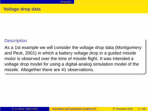
Description
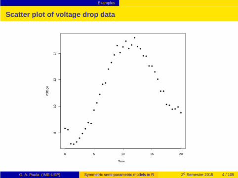
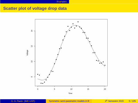
As a 1st example we will consider the voltage drop data (Montgomeryand Peck, 2001) in which a battery voltage drop in a guided missilemotor is observed over the time of missile flight. It was intended avoltage drop model for using a digital-analog simulation model of themissile. Altogether there are 41 observations.
G. A. Paula (IME-USP) Symmetric semi-parametric models in R 2o Semestre 2015 3 / 105
Examples
Scatter plot of voltage drop data
0 5 10 15 20
810
1214
Time
Volta
ge
G. A. Paula (IME-USP) Symmetric semi-parametric models in R 2o Semestre 2015 4 / 105
Examples
Scatter plot of voltage drop data
0 5 10 15 20
810
1214
Time
Volta
ge
G. A. Paula (IME-USP) Symmetric semi-parametric models in R 2o Semestre 2015 5 / 105
Examples
Possible model
Description
The data suggest a nonparametric model such as:
Voltagei = α+ f (Timei) + ǫi ,
G. A. Paula (IME-USP) Symmetric semi-parametric models in R 2o Semestre 2015 6 / 105
Examples
Possible model
Description
The data suggest a nonparametric model such as:
Voltagei = α+ f (Timei) + ǫi ,
where ǫi∼ N(0, σ2) for i = 1, . . . , 41, with f (·) being a continuous,smooth and nonparametric function.
G. A. Paula (IME-USP) Symmetric semi-parametric models in R 2o Semestre 2015 6 / 105
Examples
Boston housing data
Description
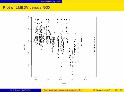
As a 2nd example we will consider the Boston housing data that havebeen analyzed by various authors (see, for instance, Belsley et al.1980). The aim of the study is to assess the association of houseprices with the air quality of the neighborhood by using regressionmodels. The outcome variable
G. A. Paula (IME-USP) Symmetric semi-parametric models in R 2o Semestre 2015 7 / 105
Examples
Boston housing data
Description
As a 2nd example we will consider the Boston housing data that havebeen analyzed by various authors (see, for instance, Belsley et al.1980). The aim of the study is to assess the association of houseprices with the air quality of the neighborhood by using regressionmodels. The outcome variable
LMEDV (logarithm of the median house price in USD 1000)
is related with 13 explanatory variables. Altogether there are 506observations.
G. A. Paula (IME-USP) Symmetric semi-parametric models in R 2o Semestre 2015 7 / 105
Examples
Boston housing data
Illustration
We will work, for the purpose of motivating the semi-parametricmodels, with three explanatory variables:
G. A. Paula (IME-USP) Symmetric semi-parametric models in R 2o Semestre 2015 8 / 105
Examples
Boston housing data
Illustration
We will work, for the purpose of motivating the semi-parametricmodels, with three explanatory variables:
NOX (annual average nitric oxide concentration, p.p. 10 million);
G. A. Paula (IME-USP) Symmetric semi-parametric models in R 2o Semestre 2015 8 / 105
Examples
Boston housing data
Illustration
We will work, for the purpose of motivating the semi-parametricmodels, with three explanatory variables:
NOX (annual average nitric oxide concentration, p.p. 10 million);
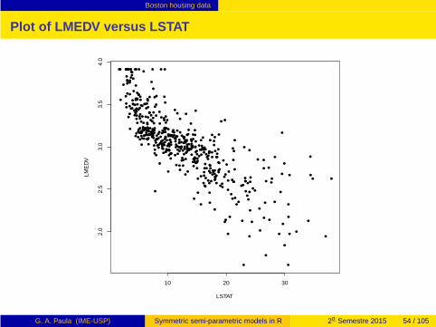
LSTAT (% lower status of the population);
G. A. Paula (IME-USP) Symmetric semi-parametric models in R 2o Semestre 2015 8 / 105
Examples
Boston housing data
Illustration
We will work, for the purpose of motivating the semi-parametricmodels, with three explanatory variables:
NOX (annual average nitric oxide concentration, p.p. 10 million);
LSTAT (% lower status of the population);
DIS (weighted distances to five Boston employment centers).
G. A. Paula (IME-USP) Symmetric semi-parametric models in R 2o Semestre 2015 8 / 105
Examples
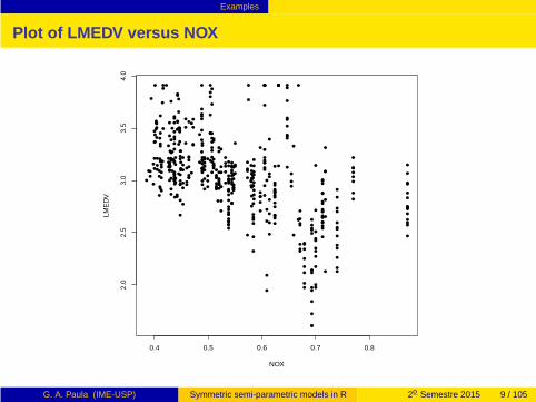
Plot of LMEDV versus NOX
0.4 0.5 0.6 0.7 0.8
2.0
2.5
3.0
3.5
4.0
NOX
LME
DV
G. A. Paula (IME-USP) Symmetric semi-parametric models in R 2o Semestre 2015 9 / 105
Examples
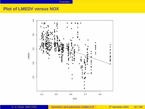
Plot of LMEDV versus NOX
0.4 0.5 0.6 0.7 0.8
2.0
2.5
3.0
3.5
4.0
NOX
LME
DV
G. A. Paula (IME-USP) Symmetric semi-parametric models in R 2o Semestre 2015 10 / 105

Examples
Plot of LMEDV versus LSTAT
10 20 30
2.0
2.5
3.0
3.5
4.0
LSTAT
LME
DV
G. A. Paula (IME-USP) Symmetric semi-parametric models in R 2o Semestre 2015 11 / 105

Examples
Plot of LMEDV versus LSTAT
10 20 30
2.0
2.5
3.0
3.5
4.0
LSTAT
LME
DV
G. A. Paula (IME-USP) Symmetric semi-parametric models in R 2o Semestre 2015 12 / 105
Examples
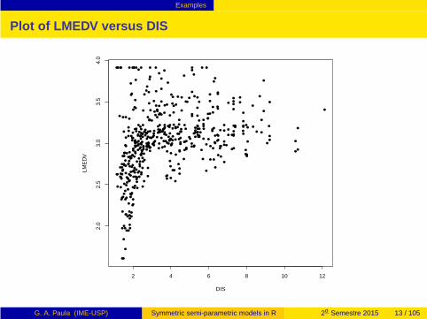
Plot of LMEDV versus DIS
2 4 6 8 10 12
2.0
2.5
3.0
3.5
4.0
DIS
LME
DV
G. A. Paula (IME-USP) Symmetric semi-parametric models in R 2o Semestre 2015 13 / 105

Examples
Plot of LMEDV versus DIS
2 4 6 8 10 12
2.0
2.5
3.0
3.5
4.0
DIS
LME
DV
G. A. Paula (IME-USP) Symmetric semi-parametric models in R 2o Semestre 2015 14 / 105
Examples
Possible model
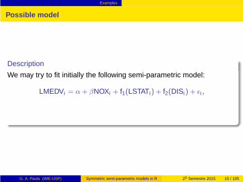
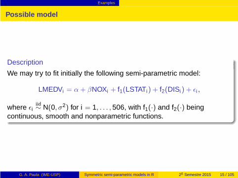
Description
We may try to fit initially the following semi-parametric model:
LMEDVi = α+ βNOXi + f1(LSTATi) + f2(DISi) + ǫi ,
G. A. Paula (IME-USP) Symmetric semi-parametric models in R 2o Semestre 2015 15 / 105
Examples
Possible model
Description
We may try to fit initially the following semi-parametric model:
LMEDVi = α+ βNOXi + f1(LSTATi) + f2(DISi) + ǫi ,
where ǫiiid∼ N(0, σ2) for i = 1, . . . , 506, with f1(·) and f2(·) being
continuous, smooth and nonparametric functions.
G. A. Paula (IME-USP) Symmetric semi-parametric models in R 2o Semestre 2015 15 / 105
Examples
Comparison of snacks
Description
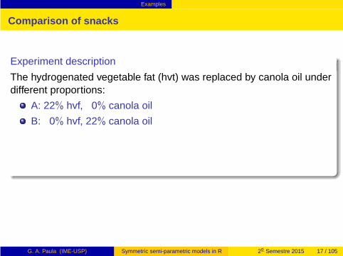
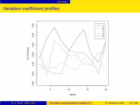
As a 3rd example, we will consider a data set from an experimentdeveloped in School of Public Health - Universidade de São Paulo, inwhich 4 different forms of light snacks (B, C, D and E) were comparedacross 20 weeks with a traditional snack (A).
G. A. Paula (IME-USP) Symmetric semi-parametric models in R 2o Semestre 2015 16 / 105

Examples
Comparison of snacks
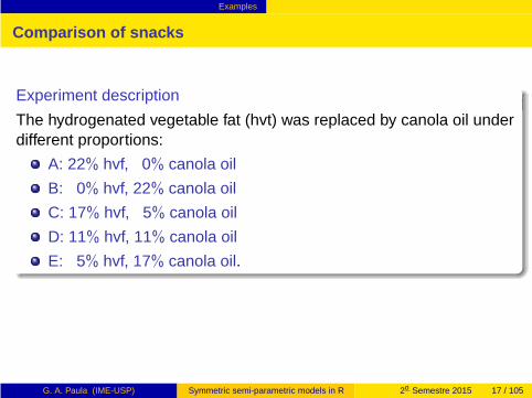
Experiment description
The hydrogenated vegetable fat (hvt) was replaced by canola oil underdifferent proportions:
G. A. Paula (IME-USP) Symmetric semi-parametric models in R 2o Semestre 2015 17 / 105

Examples
Comparison of snacks
Experiment description
The hydrogenated vegetable fat (hvt) was replaced by canola oil underdifferent proportions:
A: 22% hvf, 0% canola oil
G. A. Paula (IME-USP) Symmetric semi-parametric models in R 2o Semestre 2015 17 / 105
Examples
Comparison of snacks
Experiment description
The hydrogenated vegetable fat (hvt) was replaced by canola oil underdifferent proportions:
A: 22% hvf, 0% canola oil
B: 0% hvf, 22% canola oil
G. A. Paula (IME-USP) Symmetric semi-parametric models in R 2o Semestre 2015 17 / 105

Examples
Comparison of snacks
Experiment description
The hydrogenated vegetable fat (hvt) was replaced by canola oil underdifferent proportions:
A: 22% hvf, 0% canola oil
B: 0% hvf, 22% canola oil
C: 17% hvf, 5% canola oil
D: 11% hvf, 11% canola oil
G. A. Paula (IME-USP) Symmetric semi-parametric models in R 2o Semestre 2015 17 / 105
Examples
Comparison of snacks
Experiment description
The hydrogenated vegetable fat (hvt) was replaced by canola oil underdifferent proportions:
A: 22% hvf, 0% canola oil
B: 0% hvf, 22% canola oil
C: 17% hvf, 5% canola oil
D: 11% hvf, 11% canola oil
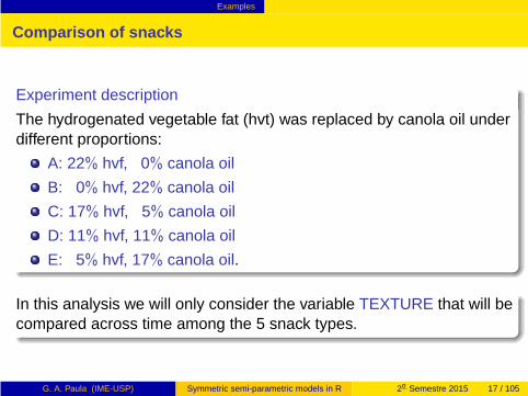
E: 5% hvf, 17% canola oil.
G. A. Paula (IME-USP) Symmetric semi-parametric models in R 2o Semestre 2015 17 / 105
Examples
Comparison of snacks
Experiment description
The hydrogenated vegetable fat (hvt) was replaced by canola oil underdifferent proportions:
A: 22% hvf, 0% canola oil
B: 0% hvf, 22% canola oil
C: 17% hvf, 5% canola oil
D: 11% hvf, 11% canola oil
E: 5% hvf, 17% canola oil.
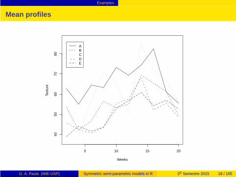
In this analysis we will only consider the variable TEXTURE that will becompared across time among the 5 snack types.
G. A. Paula (IME-USP) Symmetric semi-parametric models in R 2o Semestre 2015 17 / 105
Examples
Mean profiles
5 10 15 20
4050
6070
80
Weeks
Text
ure
ABCDE
G. A. Paula (IME-USP) Symmetric semi-parametric models in R 2o Semestre 2015 18 / 105
Examples
Variation coefficient profiles
5 10 15 20
0.05
0.10
0.15
0.20
0.25
0.30
0.35
Weeks
VC
of T
extu
reABCDE
G. A. Paula (IME-USP) Symmetric semi-parametric models in R 2o Semestre 2015 19 / 105
Examples
Double gamma model
Description
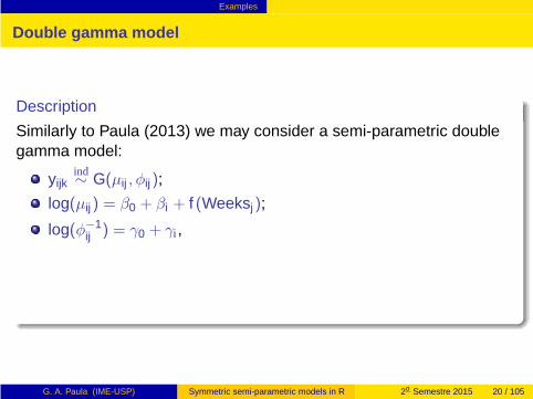
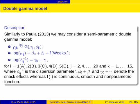
Similarly to Paula (2013) we may consider a semi-parametric doublegamma model:
G. A. Paula (IME-USP) Symmetric semi-parametric models in R 2o Semestre 2015 20 / 105
Examples
Double gamma model
Description
Similarly to Paula (2013) we may consider a semi-parametric doublegamma model:
yijkind∼ G(µij , φij);
G. A. Paula (IME-USP) Symmetric semi-parametric models in R 2o Semestre 2015 20 / 105
Examples
Double gamma model
Description
Similarly to Paula (2013) we may consider a semi-parametric doublegamma model:
yijkind∼ G(µij , φij);
log(µij) = β0 + βi + f (Weeksj);
G. A. Paula (IME-USP) Symmetric semi-parametric models in R 2o Semestre 2015 20 / 105
Examples
Double gamma model
Description
Similarly to Paula (2013) we may consider a semi-parametric doublegamma model:
yijkind∼ G(µij , φij);
log(µij) = β0 + βi + f (Weeksj);
log(φ−1ij ) = γ0 + γi ,
G. A. Paula (IME-USP) Symmetric semi-parametric models in R 2o Semestre 2015 20 / 105
Examples
Double gamma model
Description
Similarly to Paula (2013) we may consider a semi-parametric doublegamma model:
yijkind∼ G(µij , φij);
log(µij) = β0 + βi + f (Weeksj);
log(φ−1ij ) = γ0 + γi ,
for i = 1(A), 2(B), 3(C), 4(D), 5(E), j = 2, 4, . . . , 20 and k = 1, . . . , 15,where φ−1
ij is the dispersion parameter, β0 + βi and γ0 + γi denote thesnack effects whereas f (·) is continuous, smooth and nonparametricfunction.
G. A. Paula (IME-USP) Symmetric semi-parametric models in R 2o Semestre 2015 20 / 105
Defining f (x)
Outline
1 Examples
2 Defining f (x)
3 Additive normal model
4 Semi-parametric normal model
5 Packages in R
6 Voltage drop data
7 Boston housing data
8 Symmetric distributions
9 Boston housing data
10 Extensions available in the library ssym
11 Comparison of snacks
12 Bibliography
G. A. Paula (IME-USP) Symmetric semi-parametric models in R 2o Semestre 2015 21 / 105
Defining f (x)
Defining f (x)
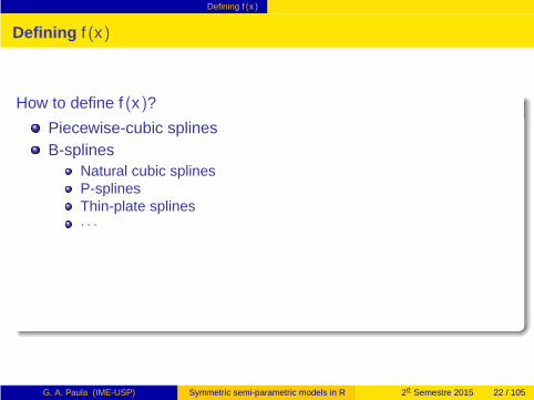
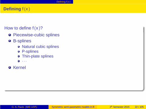
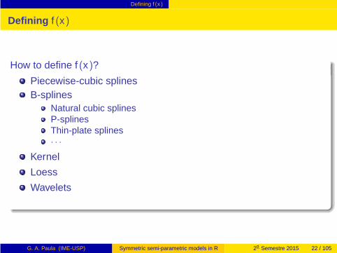
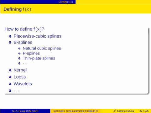
How to define f (x)?
G. A. Paula (IME-USP) Symmetric semi-parametric models in R 2o Semestre 2015 22 / 105
Defining f (x)
Defining f (x)
How to define f (x)?
Piecewise-cubic splines
G. A. Paula (IME-USP) Symmetric semi-parametric models in R 2o Semestre 2015 22 / 105
Defining f (x)
Defining f (x)
How to define f (x)?
Piecewise-cubic splinesB-splines
G. A. Paula (IME-USP) Symmetric semi-parametric models in R 2o Semestre 2015 22 / 105
Defining f (x)
Defining f (x)
How to define f (x)?
Piecewise-cubic splinesB-splines
Natural cubic splines
G. A. Paula (IME-USP) Symmetric semi-parametric models in R 2o Semestre 2015 22 / 105
Defining f (x)
Defining f (x)
How to define f (x)?
Piecewise-cubic splinesB-splines
Natural cubic splinesP-splines
G. A. Paula (IME-USP) Symmetric semi-parametric models in R 2o Semestre 2015 22 / 105

Defining f (x)
Defining f (x)
How to define f (x)?
Piecewise-cubic splinesB-splines
Natural cubic splinesP-splinesThin-plate splines
G. A. Paula (IME-USP) Symmetric semi-parametric models in R 2o Semestre 2015 22 / 105
Defining f (x)
Defining f (x)
How to define f (x)?
Piecewise-cubic splinesB-splines
Natural cubic splinesP-splinesThin-plate splines· · ·
G. A. Paula (IME-USP) Symmetric semi-parametric models in R 2o Semestre 2015 22 / 105
Defining f (x)
Defining f (x)
How to define f (x)?
Piecewise-cubic splinesB-splines
Natural cubic splinesP-splinesThin-plate splines· · ·
Kernel
G. A. Paula (IME-USP) Symmetric semi-parametric models in R 2o Semestre 2015 22 / 105

Defining f (x)
Defining f (x)
How to define f (x)?
Piecewise-cubic splinesB-splines
Natural cubic splinesP-splinesThin-plate splines· · ·
Kernel
Loess
G. A. Paula (IME-USP) Symmetric semi-parametric models in R 2o Semestre 2015 22 / 105
Defining f (x)
Defining f (x)
How to define f (x)?
Piecewise-cubic splinesB-splines
Natural cubic splinesP-splinesThin-plate splines· · ·
Kernel
Loess
Wavelets
G. A. Paula (IME-USP) Symmetric semi-parametric models in R 2o Semestre 2015 22 / 105
Defining f (x)
Defining f (x)
How to define f (x)?
Piecewise-cubic splinesB-splines
Natural cubic splinesP-splinesThin-plate splines· · ·
Kernel
Loess
Wavelets
· · ·
G. A. Paula (IME-USP) Symmetric semi-parametric models in R 2o Semestre 2015 22 / 105

Defining f (x)
Piecewise-cubic splines
Definition
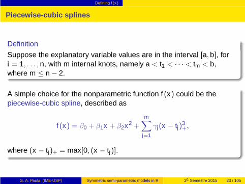
Suppose the explanatory variable values are in the interval [a, b], fori = 1, . . . , n, with m internal knots, namely a < t1 < · · · < tm < b,where m ≤ n − 2.
G. A. Paula (IME-USP) Symmetric semi-parametric models in R 2o Semestre 2015 23 / 105
Defining f (x)
Piecewise-cubic splines
Definition
Suppose the explanatory variable values are in the interval [a, b], fori = 1, . . . , n, with m internal knots, namely a < t1 < · · · < tm < b,where m ≤ n − 2.
A simple choice for the nonparametric function f (x) could be thepiecewise-cubic spline, described as
f (x) = β0 + β1x + β2x2 +
m∑
j=1
γj(x − tj)3+,
where (x − tj)+ = max[0, (x − tj)].
G. A. Paula (IME-USP) Symmetric semi-parametric models in R 2o Semestre 2015 23 / 105
Defining f (x)
Voltage drop data
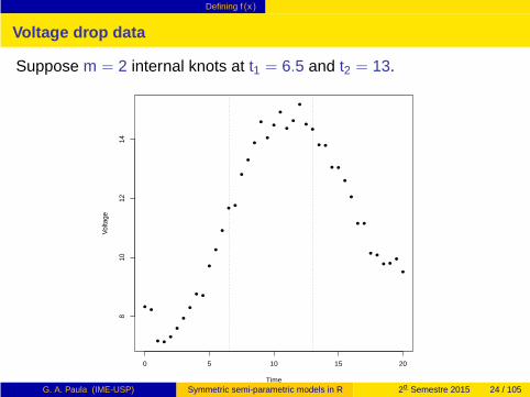
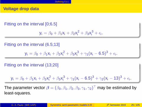
Suppose m = 2 internal knots at t1 = 6.5 and t2 = 13.
G. A. Paula (IME-USP) Symmetric semi-parametric models in R 2o Semestre 2015 24 / 105
Defining f (x)
Voltage drop data
Suppose m = 2 internal knots at t1 = 6.5 and t2 = 13.
0 5 10 15 20
810
1214
Time
Volta
ge
G. A. Paula (IME-USP) Symmetric semi-parametric models in R 2o Semestre 2015 24 / 105
Defining f (x)
Voltage drop data
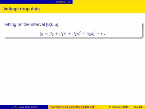
Fitting on the interval [0;6.5]
G. A. Paula (IME-USP) Symmetric semi-parametric models in R 2o Semestre 2015 25 / 105
Defining f (x)
Voltage drop data
Fitting on the interval [0;6.5]
yi = β0 + β1xi + β2x2i + β3x3
i + ǫi .
G. A. Paula (IME-USP) Symmetric semi-parametric models in R 2o Semestre 2015 25 / 105

Defining f (x)
Voltage drop data
Fitting on the interval [0;6.5]
yi = β0 + β1xi + β2x2i + β3x3
i + ǫi .
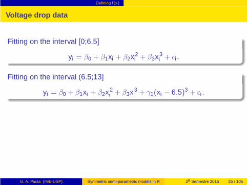
Fitting on the interval (6.5;13]
G. A. Paula (IME-USP) Symmetric semi-parametric models in R 2o Semestre 2015 25 / 105
Defining f (x)
Voltage drop data
Fitting on the interval [0;6.5]
yi = β0 + β1xi + β2x2i + β3x3
i + ǫi .
Fitting on the interval (6.5;13]
yi = β0 + β1xi + β2x2i + β3x3
i + γ1(xi − 6.5)3 + ǫi .
G. A. Paula (IME-USP) Symmetric semi-parametric models in R 2o Semestre 2015 25 / 105
Defining f (x)
Voltage drop data
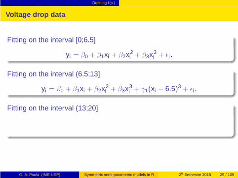
Fitting on the interval [0;6.5]
yi = β0 + β1xi + β2x2i + β3x3
i + ǫi .
Fitting on the interval (6.5;13]
yi = β0 + β1xi + β2x2i + β3x3
i + γ1(xi − 6.5)3 + ǫi .
Fitting on the interval (13;20]
G. A. Paula (IME-USP) Symmetric semi-parametric models in R 2o Semestre 2015 25 / 105
Defining f (x)
Voltage drop data
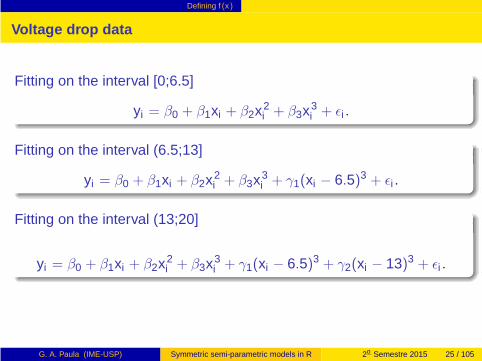
Fitting on the interval [0;6.5]
yi = β0 + β1xi + β2x2i + β3x3
i + ǫi .
Fitting on the interval (6.5;13]
yi = β0 + β1xi + β2x2i + β3x3
i + γ1(xi − 6.5)3 + ǫi .
Fitting on the interval (13;20]
yi = β0 + β1xi + β2x2i + β3x3
i + γ1(xi − 6.5)3 + γ2(xi − 13)3 + ǫi .
G. A. Paula (IME-USP) Symmetric semi-parametric models in R 2o Semestre 2015 25 / 105
Defining f (x)
Voltage drop data
Fitting on the interval [0;6.5]
yi = β0 + β1xi + β2x2i + β3x3
i + ǫi .
Fitting on the interval (6.5;13]
yi = β0 + β1xi + β2x2i + β3x3
i + γ1(xi − 6.5)3 + ǫi .
Fitting on the interval (13;20]
yi = β0 + β1xi + β2x2i + β3x3
i + γ1(xi − 6.5)3 + γ2(xi − 13)3 + ǫi .
The parameter vector β = (β0, β1, β2, β3, γ1, γ2)⊤ may be estimated by
least-squares.
G. A. Paula (IME-USP) Symmetric semi-parametric models in R 2o Semestre 2015 25 / 105
Defining f (x)
B-splines
Definition
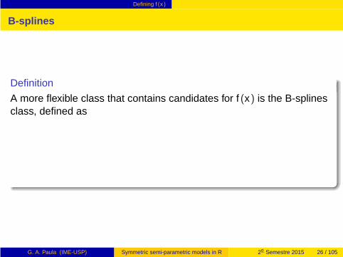
A more flexible class that contains candidates for f (x) is the B-splinesclass, defined as
G. A. Paula (IME-USP) Symmetric semi-parametric models in R 2o Semestre 2015 26 / 105
Defining f (x)
B-splines
Definition
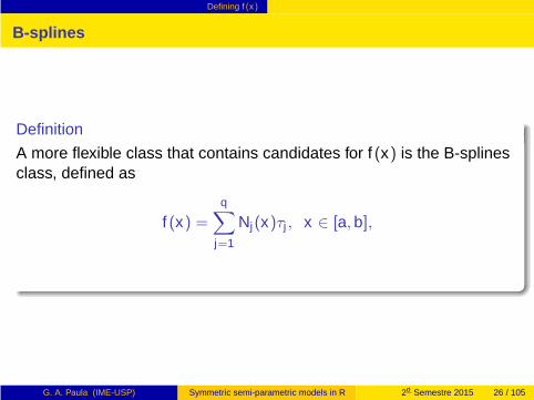
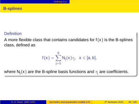
A more flexible class that contains candidates for f (x) is the B-splinesclass, defined as
f (x) =q
∑
j=1
Nj(x)τj , x ∈ [a, b],
G. A. Paula (IME-USP) Symmetric semi-parametric models in R 2o Semestre 2015 26 / 105
Defining f (x)
B-splines
Definition
A more flexible class that contains candidates for f (x) is the B-splinesclass, defined as
f (x) =q
∑
j=1
Nj(x)τj , x ∈ [a, b],
where Nj(x) are the B-spline basis functions and τj are coefficients.
G. A. Paula (IME-USP) Symmetric semi-parametric models in R 2o Semestre 2015 26 / 105

Defining f (x)
Natural cubic splines
Definition
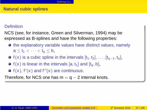
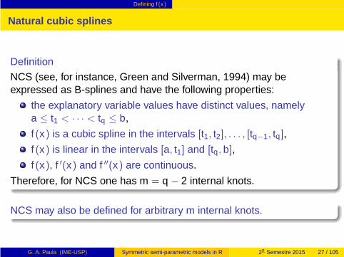
NCS (see, for instance, Green and Silverman, 1994) may beexpressed as B-splines and have the following properties:
G. A. Paula (IME-USP) Symmetric semi-parametric models in R 2o Semestre 2015 27 / 105
Defining f (x)
Natural cubic splines
Definition
NCS (see, for instance, Green and Silverman, 1994) may beexpressed as B-splines and have the following properties:
the explanatory variable values have distinct values, namelya ≤ t1 < · · · < tq ≤ b,
f (x) is a cubic spline in the intervals [t1, t2], . . . , [tq−1, tq],
f (x) is linear in the intervals [a, t1] and [tq, b],
f (x), f ′(x) and f ′′(x) are continuous.
Therefore, for NCS one has m = q − 2 internal knots.
NCS may also be defined for arbitrary m internal knots.
G. A. Paula (IME-USP) Symmetric semi-parametric models in R 2o Semestre 2015 27 / 105
Defining f (x)
P-splines
Definition
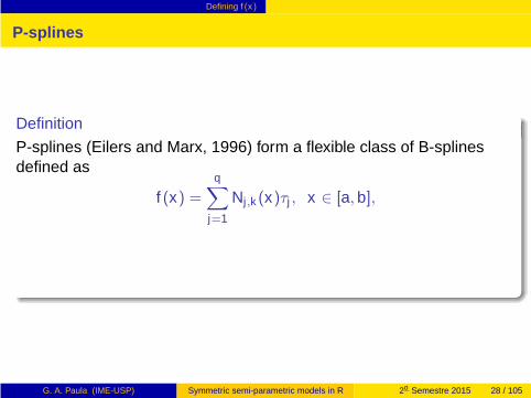
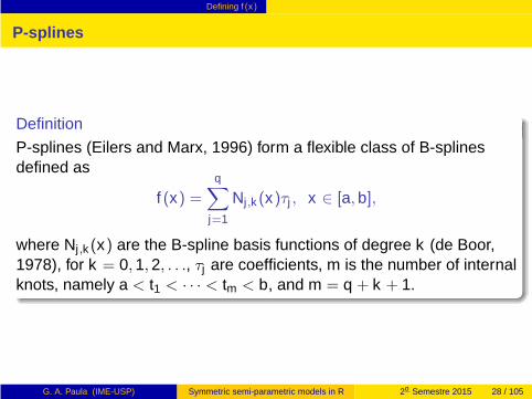
P-splines (Eilers and Marx, 1996) form a flexible class of B-splinesdefined as
G. A. Paula (IME-USP) Symmetric semi-parametric models in R 2o Semestre 2015 28 / 105
Defining f (x)
P-splines
Definition
P-splines (Eilers and Marx, 1996) form a flexible class of B-splinesdefined as
f (x) =q
∑
j=1
Nj,k (x)τj , x ∈ [a, b],
G. A. Paula (IME-USP) Symmetric semi-parametric models in R 2o Semestre 2015 28 / 105
Defining f (x)
P-splines
Definition
P-splines (Eilers and Marx, 1996) form a flexible class of B-splinesdefined as
f (x) =q
∑
j=1
Nj,k (x)τj , x ∈ [a, b],
where Nj,k (x) are the B-spline basis functions of degree k (de Boor,1978), for k = 0, 1, 2, . . ., τj are coefficients, m is the number of internalknots, namely a < t1 < · · · < tm < b, and m = q + k + 1.
G. A. Paula (IME-USP) Symmetric semi-parametric models in R 2o Semestre 2015 28 / 105
Defining f (x)
P-splines
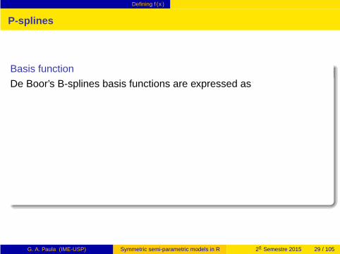
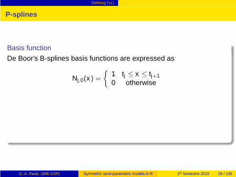
Basis function
De Boor’s B-splines basis functions are expressed as
G. A. Paula (IME-USP) Symmetric semi-parametric models in R 2o Semestre 2015 29 / 105
Defining f (x)
P-splines
Basis function
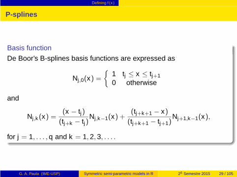
De Boor’s B-splines basis functions are expressed as
Nj,0(x) ={
1 tj ≤ x ≤ tj+1
0 otherwise
G. A. Paula (IME-USP) Symmetric semi-parametric models in R 2o Semestre 2015 29 / 105
Defining f (x)
P-splines
Basis function
De Boor’s B-splines basis functions are expressed as
Nj,0(x) ={
1 tj ≤ x ≤ tj+1
0 otherwise
and
Nj,k (x) =(x − tj)(tj+k − tj)
Nj,k−1(x) +(tj+k+1 − x)(tj+k+1 − tj+1)
Nj+1,k−1(x),
for j = 1, . . . , q and k = 1, 2, 3, . . . .
G. A. Paula (IME-USP) Symmetric semi-parametric models in R 2o Semestre 2015 29 / 105
Defining f (x)
Penalization
Why to penalize?
The aim of penalization is to reduce the parametric space solution inorder to avoid overfitting.
G. A. Paula (IME-USP) Symmetric semi-parametric models in R 2o Semestre 2015 30 / 105
Additive normal model
Outline
1 Examples
2 Defining f (x)
3 Additive normal model
4 Semi-parametric normal model
5 Packages in R
6 Voltage drop data
7 Boston housing data
8 Symmetric distributions
9 Boston housing data
10 Extensions available in the library ssym
11 Comparison of snacks
12 Bibliography
G. A. Paula (IME-USP) Symmetric semi-parametric models in R 2o Semestre 2015 31 / 105

Additive normal model
Additive normal model
Description
First, we will assume the following nonparametric model:
G. A. Paula (IME-USP) Symmetric semi-parametric models in R 2o Semestre 2015 32 / 105
Additive normal model
Additive normal model
Description
First, we will assume the following nonparametric model:
yi = f (ti) + ǫi ,
G. A. Paula (IME-USP) Symmetric semi-parametric models in R 2o Semestre 2015 32 / 105

Additive normal model
Additive normal model
Description
First, we will assume the following nonparametric model:
yi = f (ti) + ǫi ,
where f (t) is a continuous, smooth and nonparametric function and
ǫiiid∼ N(0, σ2), for i = 1, . . . , n.
G. A. Paula (IME-USP) Symmetric semi-parametric models in R 2o Semestre 2015 32 / 105
Additive normal model
Additive normal model
Penalization
A suggestion is to use the second derivative penalization.
G. A. Paula (IME-USP) Symmetric semi-parametric models in R 2o Semestre 2015 33 / 105
Additive normal model
Additive normal model
Penalization
A suggestion is to use the second derivative penalization. So, theobjective function to be minimized is given by
G. A. Paula (IME-USP) Symmetric semi-parametric models in R 2o Semestre 2015 33 / 105

Additive normal model
Additive normal model
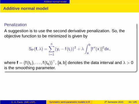
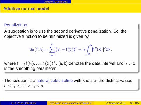
Penalization
A suggestion is to use the second derivative penalization. So, theobjective function to be minimized is given by
SP(f, λ) =n
∑
i=1
{yi − f (ti)}2 + λ
∫ b
a[f ′′(x)]2dx ,
G. A. Paula (IME-USP) Symmetric semi-parametric models in R 2o Semestre 2015 33 / 105
Additive normal model
Additive normal model
Penalization
A suggestion is to use the second derivative penalization. So, theobjective function to be minimized is given by
SP(f, λ) =n
∑
i=1
{yi − f (ti)}2 + λ
∫ b
a[f ′′(x)]2dx ,
where f = (f (t1), . . . , f (tq))⊤, [a, b] denotes the data interval and λ > 0is the smoothing parameter.
The solution is a natural cubic spline with knots at the distinct valuesa ≤ t1 < · · · < tq ≤ b.
G. A. Paula (IME-USP) Symmetric semi-parametric models in R 2o Semestre 2015 33 / 105
Additive normal model
Additive normal model
Smoothing parameter
One has the following λ interpretation:
G. A. Paula (IME-USP) Symmetric semi-parametric models in R 2o Semestre 2015 34 / 105
Additive normal model
Additive normal model
Smoothing parameter
One has the following λ interpretation:
when λ → 0 minimizing SP(f, λ) leads to a data interpolation;
G. A. Paula (IME-USP) Symmetric semi-parametric models in R 2o Semestre 2015 34 / 105
Additive normal model
Additive normal model
Smoothing parameter
One has the following λ interpretation:
when λ → 0 minimizing SP(f, λ) leads to a data interpolation;
when λ → ∞ one has to impose f ′′(x) = 0 so the solution leads toa linear function for f (x);
then 0 < λ < ∞.
G. A. Paula (IME-USP) Symmetric semi-parametric models in R 2o Semestre 2015 34 / 105

Additive normal model
Semi-parametric normal model
Penalization
One has for B-splines the following solution (see, for instance, Wood,2006):
G. A. Paula (IME-USP) Symmetric semi-parametric models in R 2o Semestre 2015 35 / 105
Additive normal model
Semi-parametric normal model
Penalization
One has for B-splines the following solution (see, for instance, Wood,2006):
∫ b
a[f ′′(x)]2dx = τ⊤Kτ ,
G. A. Paula (IME-USP) Symmetric semi-parametric models in R 2o Semestre 2015 35 / 105
Additive normal model
Semi-parametric normal model
Penalization
One has for B-splines the following solution (see, for instance, Wood,2006):
∫ b
a[f ′′(x)]2dx = τ⊤Kτ ,
where K is a (q × q) non-negative definite smoothing matrix that doesnot depend on τ .
G. A. Paula (IME-USP) Symmetric semi-parametric models in R 2o Semestre 2015 35 / 105
Semi-parametric normal model
Outline
1 Examples
2 Defining f (x)
3 Additive normal model
4 Semi-parametric normal model
5 Packages in R
6 Voltage drop data
7 Boston housing data
8 Symmetric distributions
9 Boston housing data
10 Extensions available in the library ssym
11 Comparison of snacks
12 Bibliography
G. A. Paula (IME-USP) Symmetric semi-parametric models in R 2o Semestre 2015 36 / 105

Semi-parametric normal model
Semi-parametric normal model
Description
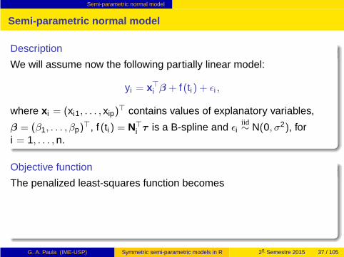
We will assume now the following partially linear model:
G. A. Paula (IME-USP) Symmetric semi-parametric models in R 2o Semestre 2015 37 / 105
Semi-parametric normal model
Semi-parametric normal model
Description
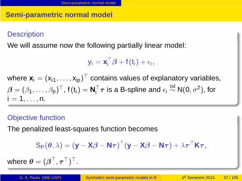
We will assume now the following partially linear model:
yi = x⊤
i β + f (ti) + ǫi ,
G. A. Paula (IME-USP) Symmetric semi-parametric models in R 2o Semestre 2015 37 / 105
Semi-parametric normal model
Semi-parametric normal model
Description
We will assume now the following partially linear model:
yi = x⊤
i β + f (ti) + ǫi ,
where x i = (xi1, . . . , xip)⊤ contains values of explanatory variables,
β = (β1, . . . , βp)⊤, f (ti) = N⊤
i τ is a B-spline and ǫiiid∼ N(0, σ2), for
i = 1, . . . , n.
Objective function
The penalized least-squares function becomes
SP(θ, λ) = (y − Xβ − Nτ )⊤(y − Xβ − Nτ ) + λτ⊤Kτ ,
where θ = (β⊤, τ⊤)⊤.
G. A. Paula (IME-USP) Symmetric semi-parametric models in R 2o Semestre 2015 37 / 105
Semi-parametric normal model
Semi-parametric normal model
Iterative process
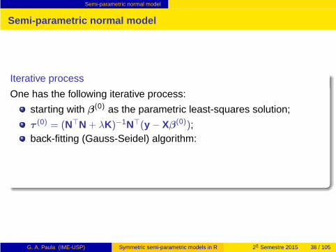
One has the following iterative process:
G. A. Paula (IME-USP) Symmetric semi-parametric models in R 2o Semestre 2015 38 / 105
Semi-parametric normal model
Semi-parametric normal model
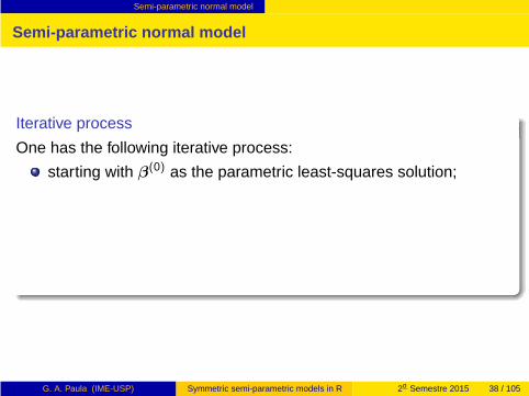
Iterative process
One has the following iterative process:
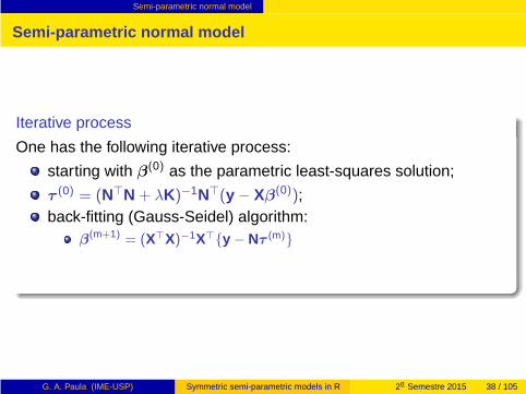
starting with β(0) as the parametric least-squares solution;
G. A. Paula (IME-USP) Symmetric semi-parametric models in R 2o Semestre 2015 38 / 105

Semi-parametric normal model
Semi-parametric normal model
Iterative process
One has the following iterative process:
starting with β(0) as the parametric least-squares solution;
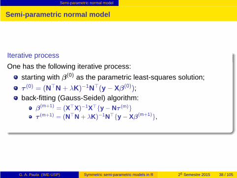
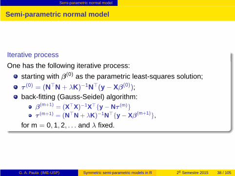
τ (0) = (N⊤N + λK)−1N⊤(y − Xβ(0));
G. A. Paula (IME-USP) Symmetric semi-parametric models in R 2o Semestre 2015 38 / 105
Semi-parametric normal model
Semi-parametric normal model
Iterative process
One has the following iterative process:
starting with β(0) as the parametric least-squares solution;
τ (0) = (N⊤N + λK)−1N⊤(y − Xβ(0));back-fitting (Gauss-Seidel) algorithm:
β(m+1) = (X⊤X)−1X⊤{y − Nτ (m)}
G. A. Paula (IME-USP) Symmetric semi-parametric models in R 2o Semestre 2015 38 / 105
Semi-parametric normal model
Semi-parametric normal model
Iterative process
One has the following iterative process:
starting with β(0) as the parametric least-squares solution;
τ (0) = (N⊤N + λK)−1N⊤(y − Xβ(0));back-fitting (Gauss-Seidel) algorithm:
β(m+1) = (X⊤X)−1X⊤{y − Nτ (m)}τ (m+1) = (N⊤N + λK)−1N⊤{y − Xβ(m+1)},
for m = 0, 1, 2, . . . and λ fixed.
G. A. Paula (IME-USP) Symmetric semi-parametric models in R 2o Semestre 2015 38 / 105
Semi-parametric normal model
Semi-parametric normal model
Effective degrees of freedom
From the iterative process at the convergence one has that
G. A. Paula (IME-USP) Symmetric semi-parametric models in R 2o Semestre 2015 39 / 105
Semi-parametric normal model
Semi-parametric normal model
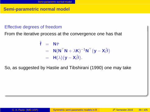
Effective degrees of freedom
From the iterative process at the convergence one has that
f = Nτ
G. A. Paula (IME-USP) Symmetric semi-parametric models in R 2o Semestre 2015 39 / 105
Semi-parametric normal model
Semi-parametric normal model
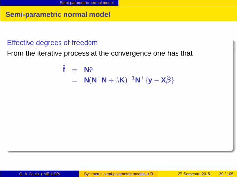
Effective degrees of freedom
From the iterative process at the convergence one has that
f = Nτ
= N(N⊤N + λK)−1N⊤{y − Xβ}
G. A. Paula (IME-USP) Symmetric semi-parametric models in R 2o Semestre 2015 39 / 105
Semi-parametric normal model
Semi-parametric normal model
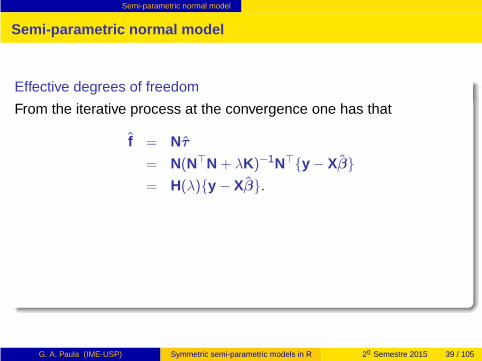
Effective degrees of freedom
From the iterative process at the convergence one has that
f = Nτ
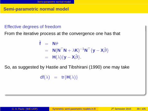
= N(N⊤N + λK)−1N⊤{y − Xβ}= H(λ){y − Xβ}.
G. A. Paula (IME-USP) Symmetric semi-parametric models in R 2o Semestre 2015 39 / 105
Semi-parametric normal model
Semi-parametric normal model
Effective degrees of freedom
From the iterative process at the convergence one has that
f = Nτ
= N(N⊤N + λK)−1N⊤{y − Xβ}= H(λ){y − Xβ}.
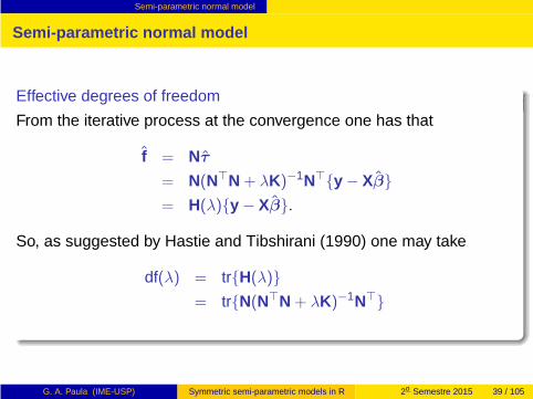
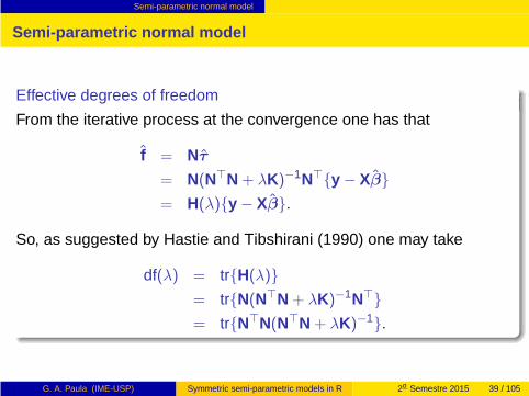
So, as suggested by Hastie and Tibshirani (1990) one may take
G. A. Paula (IME-USP) Symmetric semi-parametric models in R 2o Semestre 2015 39 / 105
Semi-parametric normal model
Semi-parametric normal model
Effective degrees of freedom
From the iterative process at the convergence one has that
f = Nτ
= N(N⊤N + λK)−1N⊤{y − Xβ}= H(λ){y − Xβ}.
So, as suggested by Hastie and Tibshirani (1990) one may take
df(λ) = tr{H(λ)}
G. A. Paula (IME-USP) Symmetric semi-parametric models in R 2o Semestre 2015 39 / 105
Semi-parametric normal model
Semi-parametric normal model
Effective degrees of freedom
From the iterative process at the convergence one has that
f = Nτ
= N(N⊤N + λK)−1N⊤{y − Xβ}= H(λ){y − Xβ}.
So, as suggested by Hastie and Tibshirani (1990) one may take
df(λ) = tr{H(λ)}= tr{N(N⊤N + λK)−1N⊤}
G. A. Paula (IME-USP) Symmetric semi-parametric models in R 2o Semestre 2015 39 / 105
Semi-parametric normal model
Semi-parametric normal model
Effective degrees of freedom
From the iterative process at the convergence one has that
f = Nτ
= N(N⊤N + λK)−1N⊤{y − Xβ}= H(λ){y − Xβ}.
So, as suggested by Hastie and Tibshirani (1990) one may take
df(λ) = tr{H(λ)}= tr{N(N⊤N + λK)−1N⊤}= tr{N⊤N(N⊤N + λK)−1}.
G. A. Paula (IME-USP) Symmetric semi-parametric models in R 2o Semestre 2015 39 / 105
Semi-parametric normal model
Semi-parametric normal model
Model selection
The Akaike Information Criterion (AIC) and the Bayesian InformationCriterion (BIC) are, respectively, defined as
G. A. Paula (IME-USP) Symmetric semi-parametric models in R 2o Semestre 2015 40 / 105

Semi-parametric normal model
Semi-parametric normal model
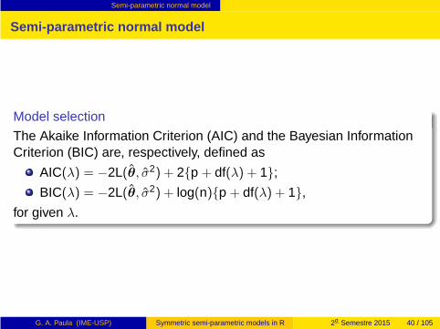
Model selection
The Akaike Information Criterion (AIC) and the Bayesian InformationCriterion (BIC) are, respectively, defined as
AIC(λ) = −2L(θ, σ2) + 2{p + df(λ) + 1};
G. A. Paula (IME-USP) Symmetric semi-parametric models in R 2o Semestre 2015 40 / 105

Semi-parametric normal model
Semi-parametric normal model
Model selection
The Akaike Information Criterion (AIC) and the Bayesian InformationCriterion (BIC) are, respectively, defined as
AIC(λ) = −2L(θ, σ2) + 2{p + df(λ) + 1};
BIC(λ) = −2L(θ, σ2) + log(n){p + df(λ) + 1},
G. A. Paula (IME-USP) Symmetric semi-parametric models in R 2o Semestre 2015 40 / 105
Semi-parametric normal model
Semi-parametric normal model
Model selection
The Akaike Information Criterion (AIC) and the Bayesian InformationCriterion (BIC) are, respectively, defined as
AIC(λ) = −2L(θ, σ2) + 2{p + df(λ) + 1};
BIC(λ) = −2L(θ, σ2) + log(n){p + df(λ) + 1},
for given λ.
G. A. Paula (IME-USP) Symmetric semi-parametric models in R 2o Semestre 2015 40 / 105
Semi-parametric normal model
Semi-parametric normal model
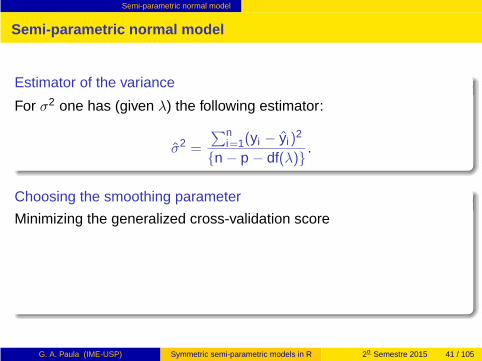
Estimator of the variance
For σ2 one has (given λ) the following estimator:
G. A. Paula (IME-USP) Symmetric semi-parametric models in R 2o Semestre 2015 41 / 105
Semi-parametric normal model
Semi-parametric normal model
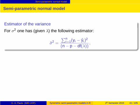
Estimator of the variance
For σ2 one has (given λ) the following estimator:
σ2 =
∑ni=1(yi − yi)
2
{n − p − df(λ)} .
G. A. Paula (IME-USP) Symmetric semi-parametric models in R 2o Semestre 2015 41 / 105
Semi-parametric normal model
Semi-parametric normal model
Estimator of the variance
For σ2 one has (given λ) the following estimator:
σ2 =
∑ni=1(yi − yi)
2
{n − p − df(λ)} .
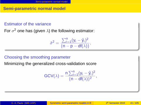
Choosing the smoothing parameter
Minimizing the generalized cross-validation score
G. A. Paula (IME-USP) Symmetric semi-parametric models in R 2o Semestre 2015 41 / 105
Semi-parametric normal model
Semi-parametric normal model
Estimator of the variance
For σ2 one has (given λ) the following estimator:
σ2 =
∑ni=1(yi − yi)
2
{n − p − df(λ)} .
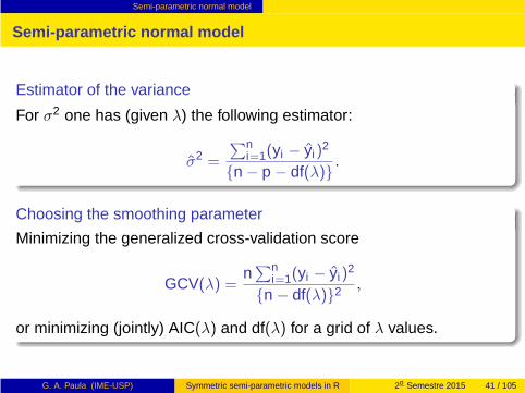
Choosing the smoothing parameter
Minimizing the generalized cross-validation score
GCV(λ) =n∑n
i=1(yi − yi)2
{n − df(λ)}2 ,
G. A. Paula (IME-USP) Symmetric semi-parametric models in R 2o Semestre 2015 41 / 105
Semi-parametric normal model
Semi-parametric normal model
Estimator of the variance
For σ2 one has (given λ) the following estimator:
σ2 =
∑ni=1(yi − yi)
2
{n − p − df(λ)} .
Choosing the smoothing parameter
Minimizing the generalized cross-validation score
GCV(λ) =n∑n
i=1(yi − yi)2
{n − df(λ)}2 ,
or minimizing (jointly) AIC(λ) and df(λ) for a grid of λ values.
G. A. Paula (IME-USP) Symmetric semi-parametric models in R 2o Semestre 2015 41 / 105
Semi-parametric normal model
Alternative penalization
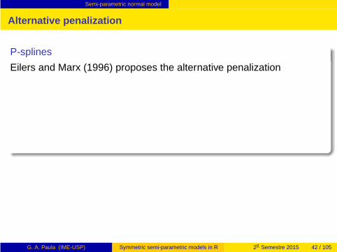
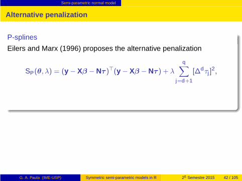
P-splines
Eilers and Marx (1996) proposes the alternative penalization
G. A. Paula (IME-USP) Symmetric semi-parametric models in R 2o Semestre 2015 42 / 105
Semi-parametric normal model
Alternative penalization
P-splines
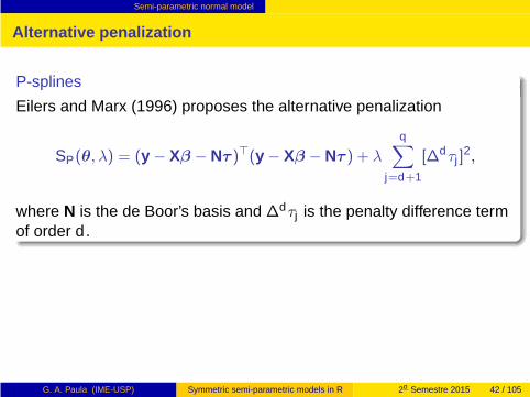
Eilers and Marx (1996) proposes the alternative penalization
SP(θ, λ) = (y − Xβ − Nτ )⊤(y − Xβ − Nτ ) + λ
q∑
j=d+1
[∆dτj ]2,
G. A. Paula (IME-USP) Symmetric semi-parametric models in R 2o Semestre 2015 42 / 105
Semi-parametric normal model
Alternative penalization
P-splines
Eilers and Marx (1996) proposes the alternative penalization
SP(θ, λ) = (y − Xβ − Nτ )⊤(y − Xβ − Nτ ) + λ
q∑
j=d+1
[∆dτj ]2,
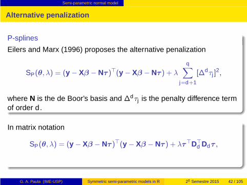
where N is the de Boor’s basis and ∆dτj is the penalty difference termof order d .
G. A. Paula (IME-USP) Symmetric semi-parametric models in R 2o Semestre 2015 42 / 105
Semi-parametric normal model
Alternative penalization
P-splines
Eilers and Marx (1996) proposes the alternative penalization
SP(θ, λ) = (y − Xβ − Nτ )⊤(y − Xβ − Nτ ) + λ
q∑
j=d+1
[∆dτj ]2,
where N is the de Boor’s basis and ∆dτj is the penalty difference termof order d .
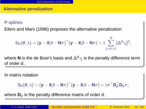
In matrix notation
SP(θ, λ) = (y − Xβ − Nτ )⊤(y − Xβ − Nτ ) + λτ⊤D⊤
d Ddτ ,
G. A. Paula (IME-USP) Symmetric semi-parametric models in R 2o Semestre 2015 42 / 105
Semi-parametric normal model
Alternative penalization
P-splines
Eilers and Marx (1996) proposes the alternative penalization
SP(θ, λ) = (y − Xβ − Nτ )⊤(y − Xβ − Nτ ) + λ
q∑
j=d+1
[∆dτj ]2,
where N is the de Boor’s basis and ∆dτj is the penalty difference termof order d .
In matrix notation
SP(θ, λ) = (y − Xβ − Nτ )⊤(y − Xβ − Nτ ) + λτ⊤D⊤
d Ddτ ,
where Dd is the penalty difference matrix of order d .
G. A. Paula (IME-USP) Symmetric semi-parametric models in R 2o Semestre 2015 42 / 105
Semi-parametric normal model
P-splines
Penalization examples
G. A. Paula (IME-USP) Symmetric semi-parametric models in R 2o Semestre 2015 43 / 105
Semi-parametric normal model
P-splines
Penalization examples
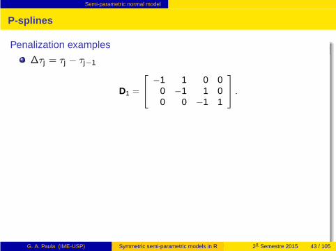
∆τj = τj − τj−1
D1 =
−1 1 0 00 −1 1 00 0 −1 1
.
G. A. Paula (IME-USP) Symmetric semi-parametric models in R 2o Semestre 2015 43 / 105
Semi-parametric normal model
P-splines
Penalization examples
∆τj = τj − τj−1
D1 =
−1 1 0 00 −1 1 00 0 −1 1
.
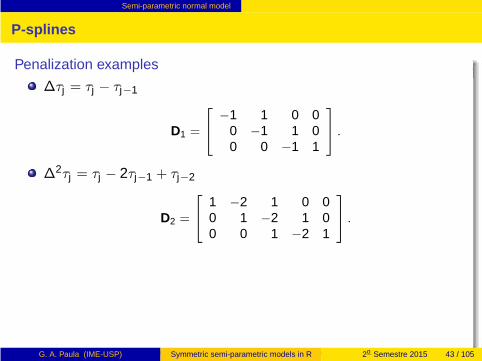
∆2τj = τj − 2τj−1 + τj−2
D2 =
1 −2 1 0 00 1 −2 1 00 0 1 −2 1
.
G. A. Paula (IME-USP) Symmetric semi-parametric models in R 2o Semestre 2015 43 / 105
Semi-parametric normal model
P-splines
Penalization examples
∆τj = τj − τj−1
D1 =
−1 1 0 00 −1 1 00 0 −1 1
.
∆2τj = τj − 2τj−1 + τj−2
D2 =
1 −2 1 0 00 1 −2 1 00 0 1 −2 1
.
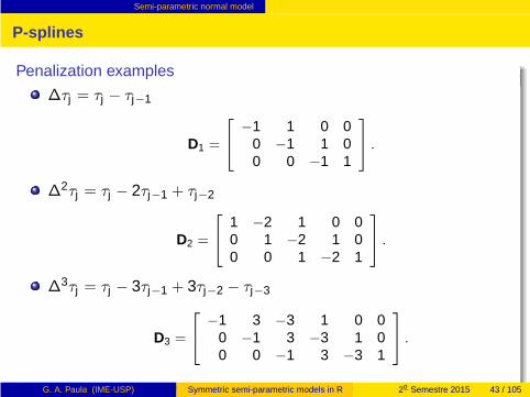
∆3τj = τj − 3τj−1 + 3τj−2 − τj−3
D3 =
−1 3 −3 1 0 00 −1 3 −3 1 00 0 −1 3 −3 1
.
G. A. Paula (IME-USP) Symmetric semi-parametric models in R 2o Semestre 2015 43 / 105
Packages in R
Outline
1 Examples
2 Defining f (x)
3 Additive normal model
4 Semi-parametric normal model
5 Packages in R
6 Voltage drop data
7 Boston housing data
8 Symmetric distributions
9 Boston housing data
10 Extensions available in the library ssym
11 Comparison of snacks
12 Bibliography
G. A. Paula (IME-USP) Symmetric semi-parametric models in R 2o Semestre 2015 44 / 105
Packages in R
Packages in R
Packages in R
Some packages for fitting semi-parametric regression models availablefrom CRAN at http://CRAN.R-project.org:
G. A. Paula (IME-USP) Symmetric semi-parametric models in R 2o Semestre 2015 45 / 105
Packages in R
Packages in R
Packages in R
Some packages for fitting semi-parametric regression models availablefrom CRAN at http://CRAN.R-project.org:
gamlss (Rigby and Stasinopoulos, 2015)
G. A. Paula (IME-USP) Symmetric semi-parametric models in R 2o Semestre 2015 45 / 105
Packages in R
Packages in R
Packages in R
Some packages for fitting semi-parametric regression models availablefrom CRAN at http://CRAN.R-project.org:
gamlss (Rigby and Stasinopoulos, 2015)
mgcv (Wood, 2015)
G. A. Paula (IME-USP) Symmetric semi-parametric models in R 2o Semestre 2015 45 / 105
Packages in R
Packages in R
Packages in R
Some packages for fitting semi-parametric regression models availablefrom CRAN at http://CRAN.R-project.org:
gamlss (Rigby and Stasinopoulos, 2015)
mgcv (Wood, 2015)
ssym (Vanegas and Paula, 2015a, 2015b)
G. A. Paula (IME-USP) Symmetric semi-parametric models in R 2o Semestre 2015 45 / 105
Voltage drop data
Outline
1 Examples
2 Defining f (x)
3 Additive normal model
4 Semi-parametric normal model
5 Packages in R
6 Voltage drop data
7 Boston housing data
8 Symmetric distributions
9 Boston housing data
10 Extensions available in the library ssym
11 Comparison of snacks
12 Bibliography
G. A. Paula (IME-USP) Symmetric semi-parametric models in R 2o Semestre 2015 46 / 105

Voltage drop data
Scatter plot of voltage drop data
0 5 10 15 20
810
1214
Time
Volta
ge
G. A. Paula (IME-USP) Symmetric semi-parametric models in R 2o Semestre 2015 47 / 105
Voltage drop data
Fitted model
Description
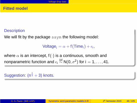
We will fit by the package ssym the following model:
Voltagei = α+ f (Timei) + ǫi ,
G. A. Paula (IME-USP) Symmetric semi-parametric models in R 2o Semestre 2015 48 / 105
Voltage drop data
Fitted model
Description
We will fit by the package ssym the following model:
Voltagei = α+ f (Timei) + ǫi ,
where α is an intercept, f (·) is a continuous, smooth and
nonparametric function and ǫiiid∼ N(0, σ2) for i = 1, . . . , 41.
Suggestion: (n13 + 3) knots.
G. A. Paula (IME-USP) Symmetric semi-parametric models in R 2o Semestre 2015 48 / 105
Voltage drop data
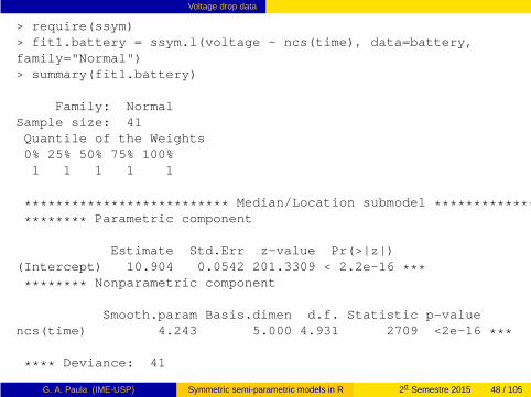
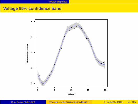
> require(ssym)> fit1.battery = ssym.l(voltage ~ ncs(time), data=battery,family="Normal")> summary(fit1.battery)
Family: NormalSample size: 41Quantile of the Weights0% 25% 50% 75% 100%1 1 1 1 1
************************** Median/Location submodel ********************************** Parametric component
Estimate Std.Err z-value Pr(>|z|)(Intercept) 10.904 0.0542 201.3309 < 2.2e-16 *********** Nonparametric component
Smooth.param Basis.dimen d.f. Statistic p-valuencs(time) 4.243 5.000 4.931 2709 <2e-16 ***
**** Deviance: 41
G. A. Paula (IME-USP) Symmetric semi-parametric models in R 2o Semestre 2015 48 / 105
Voltage drop data
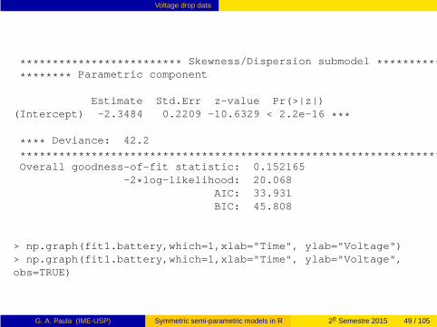
************************* Skewness/Dispersion submodel ******************************* Parametric component
Estimate Std.Err z-value Pr(>|z|)(Intercept) -2.3484 0.2209 -10.6329 < 2.2e-16 ***
**** Deviance: 42.2
*******************************************************************Overall goodness-of-fit statistic: 0.152165
-2*log-likelihood: 20.068AIC: 33.931BIC: 45.808
> np.graph(fit1.battery,which=1,xlab="Time", ylab="Voltage")> np.graph(fit1.battery,which=1,xlab="Time", ylab="Voltage",obs=TRUE)
G. A. Paula (IME-USP) Symmetric semi-parametric models in R 2o Semestre 2015 49 / 105
Voltage drop data
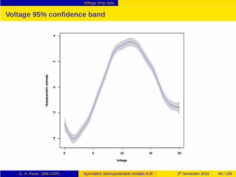
Voltage 95% confidence band
0 5 10 15 20
−4−2
02
4
Voltage
Non
para
met
ric e
stim
ate
0 5 10 15 20
−4−2
02
4
Voltage
Non
para
met
ric e
stim
ate
G. A. Paula (IME-USP) Symmetric semi-parametric models in R 2o Semestre 2015 49 / 105
Voltage drop data
Voltage 95% confidence band
0 5 10 15 20
−4−2
02
4
Voltage
Non
para
met
ric e
stim
ate
0 5 10 15 20
−4−2
02
4
0 5 10 15 20
−4−2
02
4
Voltage
Non
para
met
ric e
stim
ate
G. A. Paula (IME-USP) Symmetric semi-parametric models in R 2o Semestre 2015 50 / 105
Boston housing data
Outline
1 Examples
2 Defining f (x)
3 Additive normal model
4 Semi-parametric normal model
5 Packages in R
6 Voltage drop data
7 Boston housing data
8 Symmetric distributions
9 Boston housing data
10 Extensions available in the library ssym
11 Comparison of snacks
12 Bibliography
G. A. Paula (IME-USP) Symmetric semi-parametric models in R 2o Semestre 2015 51 / 105
Boston housing data
Plot of LMEDV versus NOX
0.4 0.5 0.6 0.7 0.8
2.0
2.5
3.0
3.5
4.0
NOX
LME
DV
G. A. Paula (IME-USP) Symmetric semi-parametric models in R 2o Semestre 2015 52 / 105

Boston housing data
Plot of LMEDV versus NOX
0.4 0.5 0.6 0.7 0.8
2.0
2.5
3.0
3.5
4.0
NOX
LME
DV
G. A. Paula (IME-USP) Symmetric semi-parametric models in R 2o Semestre 2015 53 / 105
Boston housing data
Plot of LMEDV versus LSTAT
10 20 30
2.0
2.5
3.0
3.5
4.0
LSTAT
LME
DV
G. A. Paula (IME-USP) Symmetric semi-parametric models in R 2o Semestre 2015 54 / 105

Boston housing data
Plot of LMEDV versus LSTAT
10 20 30
2.0
2.5
3.0
3.5
4.0
LSTAT
LME
DV
G. A. Paula (IME-USP) Symmetric semi-parametric models in R 2o Semestre 2015 55 / 105
Boston housing data
Possible model
Description
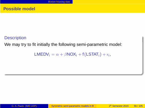
We may try to fit initially the following semi-parametric model:
LMEDVi = α+ βNOXi + f (LSTATi) + ǫi ,
G. A. Paula (IME-USP) Symmetric semi-parametric models in R 2o Semestre 2015 56 / 105
Boston housing data
Possible model
Description
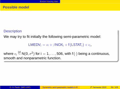
We may try to fit initially the following semi-parametric model:
LMEDVi = α+ βNOXi + f (LSTATi) + ǫi ,
where ǫiiid∼ N(0, σ2) for i = 1, . . . , 506, with f (·) being a continuous,
smooth and nonparametric function.
G. A. Paula (IME-USP) Symmetric semi-parametric models in R 2o Semestre 2015 56 / 105
Boston housing data
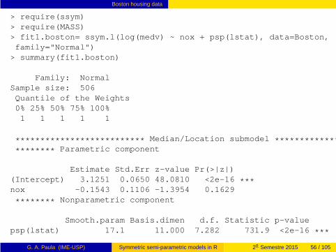
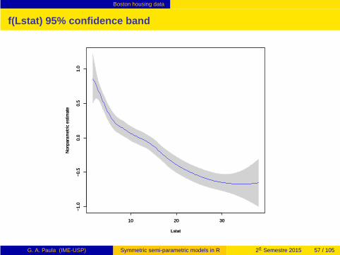
> require(ssym)> require(MASS)> fit1.boston= ssym.l(log(medv) ~ nox + psp(lstat), data=Boston,family="Normal")
> summary(fit1.boston)
Family: NormalSample size: 506Quantile of the Weights0% 25% 50% 75% 100%1 1 1 1 1
************************** Median/Location submodel ********************************** Parametric component
Estimate Std.Err z-value Pr(>|z|)(Intercept) 3.1251 0.0650 48.0810 <2e-16 ***nox -0.1543 0.1106 -1.3954 0.1629
******** Nonparametric component
Smooth.param Basis.dimen d.f. Statistic p-valuepsp(lstat) 17.1 11.000 7.282 731.9 <2e-16 ***
G. A. Paula (IME-USP) Symmetric semi-parametric models in R 2o Semestre 2015 56 / 105
Boston housing data
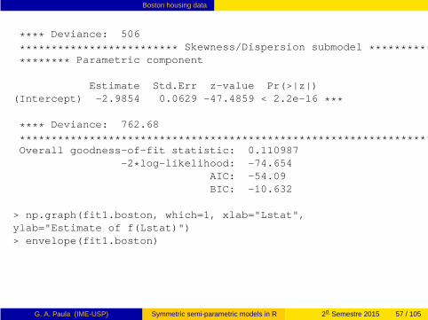
**** Deviance: 506
************************* Skewness/Dispersion submodel ******************************* Parametric component
Estimate Std.Err z-value Pr(>|z|)(Intercept) -2.9854 0.0629 -47.4859 < 2.2e-16 ***
**** Deviance: 762.68
*******************************************************************Overall goodness-of-fit statistic: 0.110987
-2*log-likelihood: -74.654AIC: -54.09BIC: -10.632
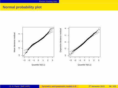
> np.graph(fit1.boston, which=1, xlab="Lstat",ylab="Estimate of f(Lstat)")> envelope(fit1.boston)
G. A. Paula (IME-USP) Symmetric semi-parametric models in R 2o Semestre 2015 57 / 105
Boston housing data
f(Lstat) 95% confidence band
10 20 30
−1.0
−0.5
0.0
0.5
1.0
Lstat
Non
para
met
ric e
stim
ate
10 20 30
−1.0
−0.5
0.0
0.5
1.0
Lstat
Non
para
met
ric e
stim
ate
G. A. Paula (IME-USP) Symmetric semi-parametric models in R 2o Semestre 2015 57 / 105
Boston housing data
Normal probability plot
−3 −2 −1 0 1 2 3
−4−2
02
Quantile N(0,1)
Mea
n de
vian
ce r
esid
ual
−3 −2 −1 0 1 2 3
−4−2
02
4Quantile N(0,1)
Dis
pers
ion
devi
ance
res
idua
l
G. A. Paula (IME-USP) Symmetric semi-parametric models in R 2o Semestre 2015 58 / 105
Symmetric distributions
Outline
1 Examples
2 Defining f (x)
3 Additive normal model
4 Semi-parametric normal model
5 Packages in R
6 Voltage drop data
7 Boston housing data
8 Symmetric distributions
9 Boston housing data
10 Extensions available in the library ssym
11 Comparison of snacks
12 Bibliography
G. A. Paula (IME-USP) Symmetric semi-parametric models in R 2o Semestre 2015 59 / 105
Symmetric distributions
Symmetric distributions
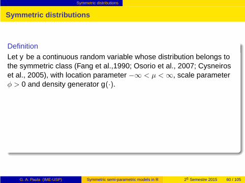
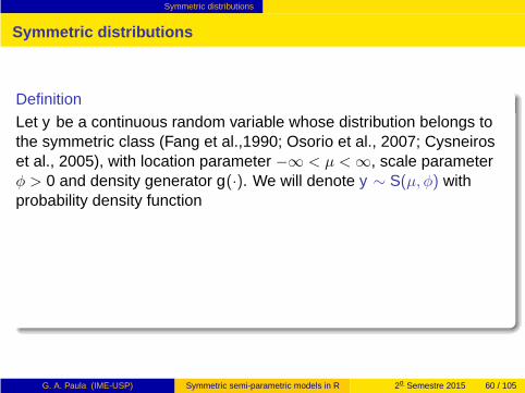
DefinitionLet y be a continuous random variable whose distribution belongs tothe symmetric class (Fang et al.,1990; Osorio et al., 2007; Cysneiroset al., 2005), with location parameter −∞ < µ < ∞, scale parameterφ > 0 and density generator g(·).
G. A. Paula (IME-USP) Symmetric semi-parametric models in R 2o Semestre 2015 60 / 105
Symmetric distributions
Symmetric distributions
DefinitionLet y be a continuous random variable whose distribution belongs tothe symmetric class (Fang et al.,1990; Osorio et al., 2007; Cysneiroset al., 2005), with location parameter −∞ < µ < ∞, scale parameterφ > 0 and density generator g(·). We will denote y ∼ S(µ, φ) withprobability density function
G. A. Paula (IME-USP) Symmetric semi-parametric models in R 2o Semestre 2015 60 / 105
Symmetric distributions
Symmetric distributions
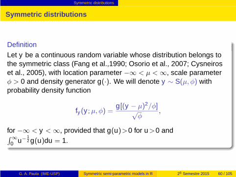
DefinitionLet y be a continuous random variable whose distribution belongs tothe symmetric class (Fang et al.,1990; Osorio et al., 2007; Cysneiroset al., 2005), with location parameter −∞ < µ < ∞, scale parameterφ > 0 and density generator g(·). We will denote y ∼ S(µ, φ) withprobability density function
fy (y ;µ, φ) =g[(y − µ)2/φ]√
φ,
for −∞ < y < ∞, provided that g(u)>0 for u>0 and∫
∞
0 u−12 g(u)du = 1.
G. A. Paula (IME-USP) Symmetric semi-parametric models in R 2o Semestre 2015 60 / 105

Symmetric distributions
Symmetric distributions
DefinitionLet y be a continuous random variable whose distribution belongs tothe symmetric class (Fang et al.,1990; Osorio et al., 2007; Cysneiroset al., 2005), with location parameter −∞ < µ < ∞, scale parameterφ > 0 and density generator g(·). We will denote y ∼ S(µ, φ) withprobability density function
fy (y ;µ, φ) =g[(y − µ)2/φ]√
φ,
for −∞ < y < ∞, provided that g(u)>0 for u>0 and∫
∞
0 u−12 g(u)du = 1.When they exist E(y) = µ and Var(y) = ξφ.
G. A. Paula (IME-USP) Symmetric semi-parametric models in R 2o Semestre 2015 60 / 105
Symmetric distributions
Symmetric distributions
Examples
G. A. Paula (IME-USP) Symmetric semi-parametric models in R 2o Semestre 2015 61 / 105
Symmetric distributions
Symmetric distributions
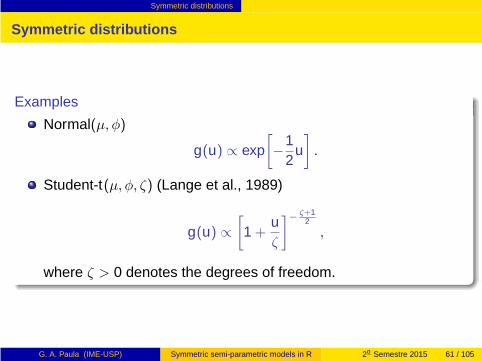
Examples
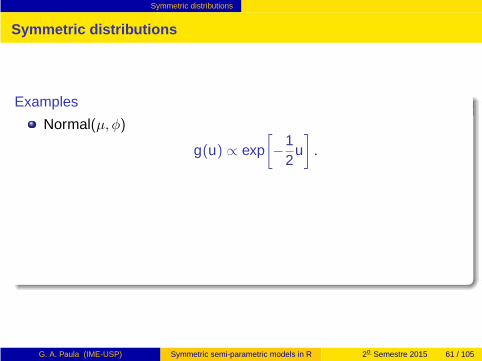
Normal(µ, φ)
g(u) ∝ exp[
−12
u]
.
G. A. Paula (IME-USP) Symmetric semi-parametric models in R 2o Semestre 2015 61 / 105
Symmetric distributions
Symmetric distributions
Examples
Normal(µ, φ)
g(u) ∝ exp[
−12
u]
.
Student-t(µ, φ, ζ) (Lange et al., 1989)
g(u) ∝[
1 +uζ
]−ζ+1
2
,
where ζ > 0 denotes the degrees of freedom.
G. A. Paula (IME-USP) Symmetric semi-parametric models in R 2o Semestre 2015 61 / 105
Symmetric distributions
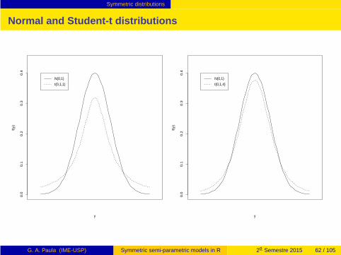
Normal and Student-t distributions0
.00
.10
.20
.30
.4
y
f(y)
N(0,1)
t(0,1,1)
0.0
0.1
0.2
0.3
0.4
y
f(y)
N(0,1)
t(0,1,4)
G. A. Paula (IME-USP) Symmetric semi-parametric models in R 2o Semestre 2015 62 / 105
Symmetric distributions
Symmetric distributions
Examples
G. A. Paula (IME-USP) Symmetric semi-parametric models in R 2o Semestre 2015 63 / 105
Symmetric distributions
Symmetric distributions
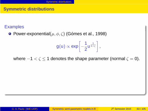
Examples
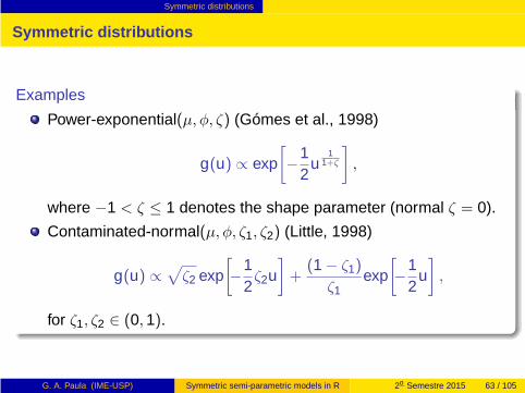
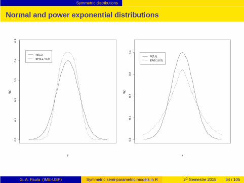
Power-exponential(µ, φ, ζ) (Gómes et al., 1998)
g(u) ∝ exp[
−12
u1
1+ζ
]
,
where −1 < ζ ≤ 1 denotes the shape parameter (normal ζ = 0).
G. A. Paula (IME-USP) Symmetric semi-parametric models in R 2o Semestre 2015 63 / 105
Symmetric distributions
Symmetric distributions
Examples
Power-exponential(µ, φ, ζ) (Gómes et al., 1998)
g(u) ∝ exp[
−12
u1
1+ζ
]
,
where −1 < ζ ≤ 1 denotes the shape parameter (normal ζ = 0).
Contaminated-normal(µ, φ, ζ1, ζ2) (Little, 1998)
g(u) ∝√
ζ2 exp[
−12ζ2u
]
+(1 − ζ1)
ζ1exp
[
−12
u]
,
for ζ1, ζ2 ∈ (0, 1).
G. A. Paula (IME-USP) Symmetric semi-parametric models in R 2o Semestre 2015 63 / 105
Symmetric distributions
Normal and power exponential distributions0
.00
.10
.20
.30
.40
.5
y
f(y)
N(0,1)
EP(0,1,−0.3)
0.0
0.1
0.2
0.3
0.4
y
f(y)
N(0,1)
EP(0,1,0.5)
G. A. Paula (IME-USP) Symmetric semi-parametric models in R 2o Semestre 2015 64 / 105

Symmetric distributions
Symmetric distributions
Examples
G. A. Paula (IME-USP) Symmetric semi-parametric models in R 2o Semestre 2015 65 / 105
Symmetric distributions
Symmetric distributions
Examples
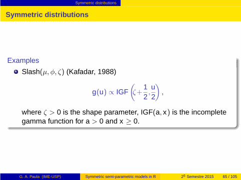
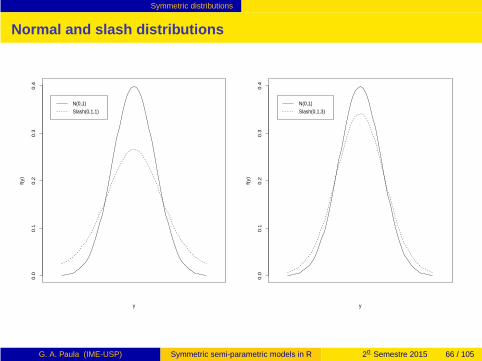
Slash(µ, φ, ζ) (Kafadar, 1988)
g(u) ∝ IGF(
ζ+12,u2
)
,
where ζ > 0 is the shape parameter, IGF(a, x) is the incompletegamma function for a > 0 and x ≥ 0.
G. A. Paula (IME-USP) Symmetric semi-parametric models in R 2o Semestre 2015 65 / 105
Symmetric distributions
Normal and slash distributions0
.00
.10
.20
.30
.4
y
f(y)
N(0,1)
Slash(0,1,1)
0.0
0.1
0.2
0.3
0.4
y
f(y)
N(0,1)
Slash(0,1,3)
G. A. Paula (IME-USP) Symmetric semi-parametric models in R 2o Semestre 2015 66 / 105
Symmetric distributions
Symmetric distributions
Examples
G. A. Paula (IME-USP) Symmetric semi-parametric models in R 2o Semestre 2015 67 / 105
Symmetric distributions
Symmetric distributions
Examples
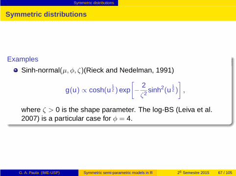
Sinh-normal(µ, φ, ζ)(Rieck and Nedelman, 1991)
g(u) ∝ cosh(u12 ) exp
[
− 2ζ2 sinh2(u
12 )
]
,
where ζ > 0 is the shape parameter. The log-BS (Leiva et al.2007) is a particular case for φ = 4.
G. A. Paula (IME-USP) Symmetric semi-parametric models in R 2o Semestre 2015 67 / 105

Symmetric distributions
Symmetric distributions
Examples
G. A. Paula (IME-USP) Symmetric semi-parametric models in R 2o Semestre 2015 68 / 105
Symmetric distributions
Symmetric distributions
Examples
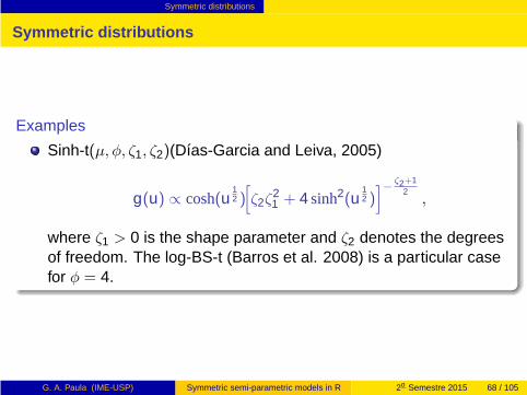
Sinh-t(µ, φ, ζ1, ζ2)(Días-Garcia and Leiva, 2005)
g(u) ∝ cosh(u12 )[
ζ2ζ21 + 4 sinh2(u
12 )]−
ζ2+12
,
where ζ1 > 0 is the shape parameter and ζ2 denotes the degreesof freedom. The log-BS-t (Barros et al. 2008) is a particular casefor φ = 4.
G. A. Paula (IME-USP) Symmetric semi-parametric models in R 2o Semestre 2015 68 / 105

Symmetric distributions
Normal and sinh-normal distributions0
.00
.20
.40
.60
.8
y
f(y)
N(0,1)
SN(0,1,1)
0.0
0.1
0.2
0.3
0.4
y
f(y)
N(0,1)
SN(0,1,3)
G. A. Paula (IME-USP) Symmetric semi-parametric models in R 2o Semestre 2015 69 / 105
Symmetric distributions
Semi-parametric symmetric models
Description
We will now consider the following partially linear model:
G. A. Paula (IME-USP) Symmetric semi-parametric models in R 2o Semestre 2015 70 / 105
Symmetric distributions
Semi-parametric symmetric models
Description
We will now consider the following partially linear model:
yi = x⊤
i β + f (ti) + ǫi
G. A. Paula (IME-USP) Symmetric semi-parametric models in R 2o Semestre 2015 70 / 105
Symmetric distributions
Semi-parametric symmetric models
Description
We will now consider the following partially linear model:
yi = x⊤
i β + f (ti) + ǫi
= x⊤
i β + N⊤
i τ + ǫi ,
G. A. Paula (IME-USP) Symmetric semi-parametric models in R 2o Semestre 2015 70 / 105
Symmetric distributions
Semi-parametric symmetric models
Description
We will now consider the following partially linear model:
yi = x⊤
i β + f (ti) + ǫi
= x⊤
i β + N⊤
i τ + ǫi ,
where x i = (xi1, . . . , xip)⊤ contains values of explanatory variables,
β = (β1, . . . , βp)⊤, f (ti) = N⊤
i τ is a B-spline, τ = (τ1, . . . , τq)⊤ and ǫi
iid∼S(0, φ), for i = 1, . . . , n.
G. A. Paula (IME-USP) Symmetric semi-parametric models in R 2o Semestre 2015 70 / 105
Symmetric distributions
Semi-parametric symmetric models
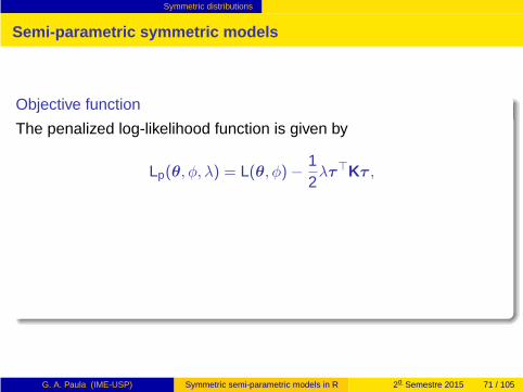
Objective function
The penalized log-likelihood function is given by
G. A. Paula (IME-USP) Symmetric semi-parametric models in R 2o Semestre 2015 71 / 105
Symmetric distributions
Semi-parametric symmetric models
Objective function
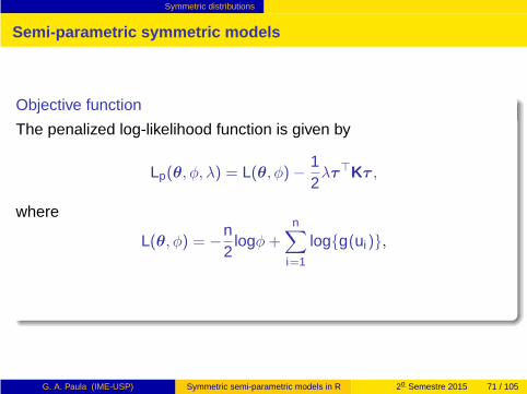
The penalized log-likelihood function is given by
Lp(θ, φ, λ) = L(θ, φ)− 12λτ⊤Kτ ,
G. A. Paula (IME-USP) Symmetric semi-parametric models in R 2o Semestre 2015 71 / 105
Symmetric distributions
Semi-parametric symmetric models
Objective function
The penalized log-likelihood function is given by
Lp(θ, φ, λ) = L(θ, φ)− 12λτ⊤Kτ ,
where
L(θ, φ) = −n2
logφ+n
∑
i=1
log{g(ui)},
G. A. Paula (IME-USP) Symmetric semi-parametric models in R 2o Semestre 2015 71 / 105

Symmetric distributions
Semi-parametric symmetric models
Objective function
The penalized log-likelihood function is given by
Lp(θ, φ, λ) = L(θ, φ)− 12λτ⊤Kτ ,
where
L(θ, φ) = −n2
logφ+n
∑
i=1
log{g(ui)},
θ = (β⊤, τ⊤)⊤, ui = (yi − µi)2/φ, λ is the smoothing parameter and K
is a positive definite matrix.
G. A. Paula (IME-USP) Symmetric semi-parametric models in R 2o Semestre 2015 71 / 105
Symmetric distributions
Semi-parametric normal model
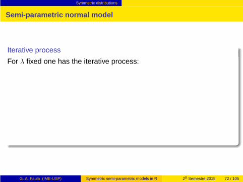
Iterative process
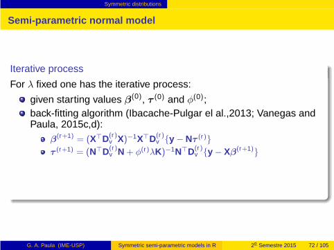
For λ fixed one has the iterative process:
G. A. Paula (IME-USP) Symmetric semi-parametric models in R 2o Semestre 2015 72 / 105

Symmetric distributions
Semi-parametric normal model
Iterative process
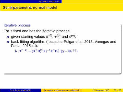
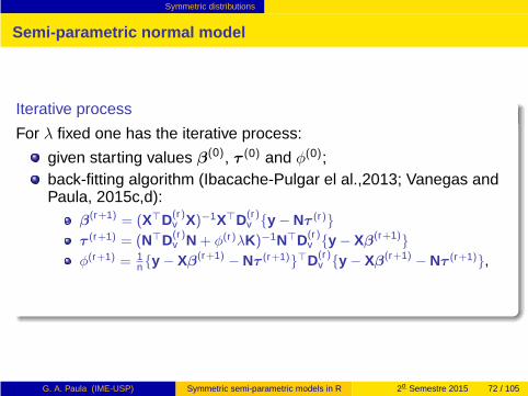
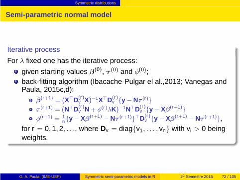
For λ fixed one has the iterative process:
given starting values β(0), τ (0) and φ(0);
G. A. Paula (IME-USP) Symmetric semi-parametric models in R 2o Semestre 2015 72 / 105

Symmetric distributions
Semi-parametric normal model
Iterative process
For λ fixed one has the iterative process:
given starting values β(0), τ (0) and φ(0);back-fitting algorithm (Ibacache-Pulgar el al.,2013; Vanegas andPaula, 2015c,d):
G. A. Paula (IME-USP) Symmetric semi-parametric models in R 2o Semestre 2015 72 / 105
Symmetric distributions
Semi-parametric normal model
Iterative process
For λ fixed one has the iterative process:
given starting values β(0), τ (0) and φ(0);back-fitting algorithm (Ibacache-Pulgar el al.,2013; Vanegas andPaula, 2015c,d):
β(r+1) = (X⊤D(r)v X)−1X⊤D(r)
v {y − Nτ (r)}
G. A. Paula (IME-USP) Symmetric semi-parametric models in R 2o Semestre 2015 72 / 105
Symmetric distributions
Semi-parametric normal model
Iterative process
For λ fixed one has the iterative process:
given starting values β(0), τ (0) and φ(0);back-fitting algorithm (Ibacache-Pulgar el al.,2013; Vanegas andPaula, 2015c,d):
β(r+1) = (X⊤D(r)v X)−1X⊤D(r)
v {y − Nτ (r)}τ (r+1) = (N⊤D(r)
v N + φ(r)λK)−1N⊤D(r)v {y − Xβ(r+1)}
φ(r+1) = 1n{y − Xβ(r+1) − Nτ (r+1)}⊤D(r)
v {y − Xβ(r+1) − Nτ (r+1)},
for r = 0, 1, 2, . . ., where Dv = diag{v1, . . . , vn} with vi > 0 beingweights.
G. A. Paula (IME-USP) Symmetric semi-parametric models in R 2o Semestre 2015 72 / 105
Symmetric distributions
Semi-parametric symmetric models
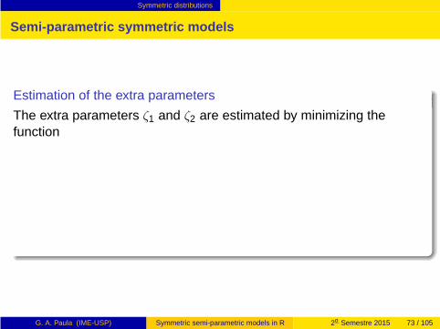
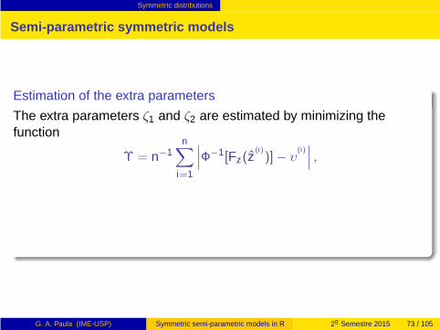
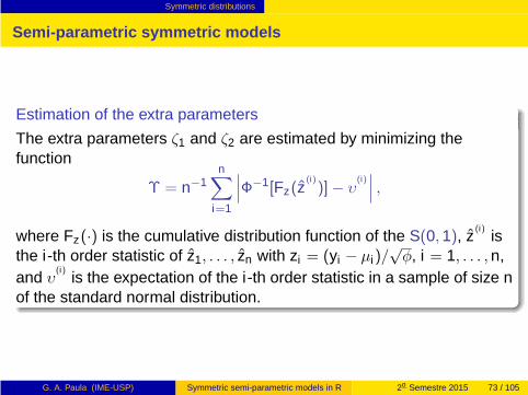
Estimation of the extra parameters
The extra parameters ζ1 and ζ2 are estimated by minimizing thefunction
G. A. Paula (IME-USP) Symmetric semi-parametric models in R 2o Semestre 2015 73 / 105
Symmetric distributions
Semi-parametric symmetric models
Estimation of the extra parameters
The extra parameters ζ1 and ζ2 are estimated by minimizing thefunction
Υ = n−1n
∑
i=1
∣
∣
∣Φ−1[Fz(z
(i))]− υ
(i)∣
∣
∣,
G. A. Paula (IME-USP) Symmetric semi-parametric models in R 2o Semestre 2015 73 / 105
Symmetric distributions
Semi-parametric symmetric models
Estimation of the extra parameters
The extra parameters ζ1 and ζ2 are estimated by minimizing thefunction
Υ = n−1n
∑
i=1
∣
∣
∣Φ−1[Fz(z
(i))]− υ
(i)∣
∣
∣,
where Fz(·) is the cumulative distribution function of the S(0, 1), z(i)
isthe i-th order statistic of z1, . . . , zn with zi = (yi − µi)/
√φ, i = 1, . . . , n,
and υ(i)
is the expectation of the i-th order statistic in a sample of size nof the standard normal distribution.
G. A. Paula (IME-USP) Symmetric semi-parametric models in R 2o Semestre 2015 73 / 105
Symmetric distributions
Semi-parametric symmetric models
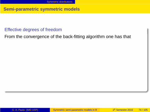
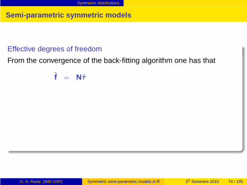
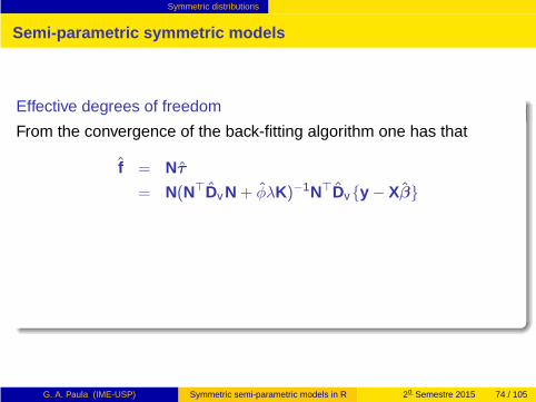
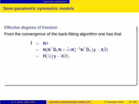
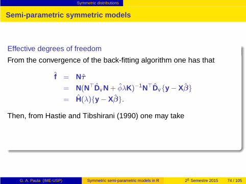
Effective degrees of freedom
From the convergence of the back-fitting algorithm one has that
G. A. Paula (IME-USP) Symmetric semi-parametric models in R 2o Semestre 2015 74 / 105
Symmetric distributions
Semi-parametric symmetric models
Effective degrees of freedom
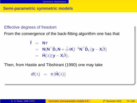
From the convergence of the back-fitting algorithm one has that
f = Nτ
G. A. Paula (IME-USP) Symmetric semi-parametric models in R 2o Semestre 2015 74 / 105
Symmetric distributions
Semi-parametric symmetric models
Effective degrees of freedom
From the convergence of the back-fitting algorithm one has that
f = Nτ
= N(N⊤Dv N + φλK)−1N⊤Dv{y − Xβ}
G. A. Paula (IME-USP) Symmetric semi-parametric models in R 2o Semestre 2015 74 / 105
Symmetric distributions
Semi-parametric symmetric models
Effective degrees of freedom
From the convergence of the back-fitting algorithm one has that
f = Nτ
= N(N⊤Dv N + φλK)−1N⊤Dv{y − Xβ}= H(λ){y − Xβ}.
G. A. Paula (IME-USP) Symmetric semi-parametric models in R 2o Semestre 2015 74 / 105
Symmetric distributions
Semi-parametric symmetric models
Effective degrees of freedom
From the convergence of the back-fitting algorithm one has that
f = Nτ
= N(N⊤Dv N + φλK)−1N⊤Dv{y − Xβ}= H(λ){y − Xβ}.
Then, from Hastie and Tibshirani (1990) one may take
df(λ) = tr{H(λ)}
G. A. Paula (IME-USP) Symmetric semi-parametric models in R 2o Semestre 2015 74 / 105

Symmetric distributions
Semi-parametric symmetric models
Effective degrees of freedom
From the convergence of the back-fitting algorithm one has that
f = Nτ
= N(N⊤Dv N + φλK)−1N⊤Dv{y − Xβ}= H(λ){y − Xβ}.
Then, from Hastie and Tibshirani (1990) one may take
df(λ) = tr{H(λ)}= tr{N⊤Dv N(N⊤Dv N + φλK)−1}.
G. A. Paula (IME-USP) Symmetric semi-parametric models in R 2o Semestre 2015 74 / 105
Symmetric distributions
Semi-parametric symmetric models
G. A. Paula (IME-USP) Symmetric semi-parametric models in R 2o Semestre 2015 75 / 105
Symmetric distributions
Semi-parametric symmetric models
Model selection
The Akaike Information Criterion (AIC) and the Bayesian InformationCriterion (BIC) are, respectively, defined as
AIC(λ) = −2L(θ, φ) + 2{p + df(λ) + 1};
BIC(λ) = −2L(θ φ) + log(n){p + df(λ) + 1},
G. A. Paula (IME-USP) Symmetric semi-parametric models in R 2o Semestre 2015 75 / 105

Symmetric distributions
Semi-parametric symmetric models
Model selection
The Akaike Information Criterion (AIC) and the Bayesian InformationCriterion (BIC) are, respectively, defined as
AIC(λ) = −2L(θ, φ) + 2{p + df(λ) + 1};
BIC(λ) = −2L(θ φ) + log(n){p + df(λ) + 1},
for given λ.
G. A. Paula (IME-USP) Symmetric semi-parametric models in R 2o Semestre 2015 75 / 105
Symmetric distributions
Semi-parametric symmetric models
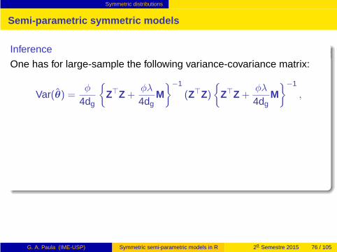
Inference
One has for large-sample the following variance-covariance matrix:
G. A. Paula (IME-USP) Symmetric semi-parametric models in R 2o Semestre 2015 76 / 105
Symmetric distributions
Semi-parametric symmetric models
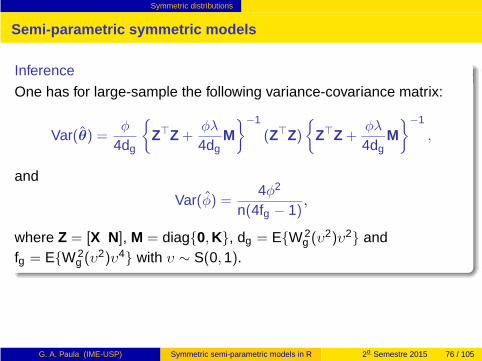
Inference
One has for large-sample the following variance-covariance matrix:
Var(θ) =φ
4dg
{
Z⊤Z +φλ
4dgM}−1
(Z⊤Z){
Z⊤Z +φλ
4dgM}−1
,
G. A. Paula (IME-USP) Symmetric semi-parametric models in R 2o Semestre 2015 76 / 105

Symmetric distributions
Semi-parametric symmetric models
Inference
One has for large-sample the following variance-covariance matrix:
Var(θ) =φ
4dg
{
Z⊤Z +φλ
4dgM}−1
(Z⊤Z){
Z⊤Z +φλ
4dgM}−1
,
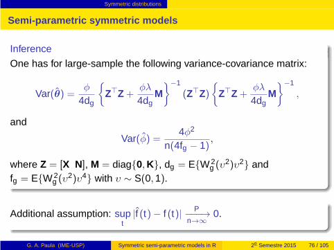
and
Var(φ) =4φ2
n(4fg − 1),
G. A. Paula (IME-USP) Symmetric semi-parametric models in R 2o Semestre 2015 76 / 105
Symmetric distributions
Semi-parametric symmetric models
Inference
One has for large-sample the following variance-covariance matrix:
Var(θ) =φ
4dg
{
Z⊤Z +φλ
4dgM}−1
(Z⊤Z){
Z⊤Z +φλ
4dgM}−1
,
and
Var(φ) =4φ2
n(4fg − 1),
where Z = [X N], M = diag{0,K}, dg = E{W 2g (υ
2)υ2} andfg = E{W 2
g (υ2)υ4} with υ ∼ S(0, 1).
Additional assumption: supt
|f (t)− f (t)| P−−−→n→∞
0.
G. A. Paula (IME-USP) Symmetric semi-parametric models in R 2o Semestre 2015 76 / 105
Symmetric distributions
Semi-parametric symmetric models
Residuals
G. A. Paula (IME-USP) Symmetric semi-parametric models in R 2o Semestre 2015 77 / 105
Symmetric distributions
Semi-parametric symmetric models
Residualsquantile residual
qi = Φ−1[Fz(z(i))].
G. A. Paula (IME-USP) Symmetric semi-parametric models in R 2o Semestre 2015 77 / 105
Symmetric distributions
Semi-parametric symmetric models
Residualsquantile residual
qi = Φ−1[Fz(z(i))].
mean deviance residual
tµ(zi) = sign(zi)[
di(µ|φ)]
12,
where di(µ|φ) is the the i-th log-likelihood difference given φ.
dispersion deviance residual
tφ(zi) = sign(zi)[
di(φ|µ)]
12,
where di(φ|µ) is the the i-th log-likelihood difference given µ.
G. A. Paula (IME-USP) Symmetric semi-parametric models in R 2o Semestre 2015 77 / 105

Symmetric distributions
Semi-parametric symmetric models
Sensitivity analysis
In order to assess the influence of small perturbations in the model ordata on the parameter estimates we may apply the Local InfluenceApproach (Cook, 1986; Poon and Poon, 1999).
G. A. Paula (IME-USP) Symmetric semi-parametric models in R 2o Semestre 2015 78 / 105
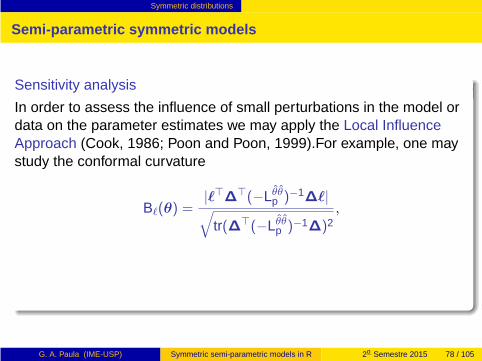
Symmetric distributions
Semi-parametric symmetric models
Sensitivity analysis
In order to assess the influence of small perturbations in the model ordata on the parameter estimates we may apply the Local InfluenceApproach (Cook, 1986; Poon and Poon, 1999).For example, one maystudy the conformal curvature
Bℓ(θ) =|ℓ⊤∆⊤(−Lθθ
p )−1∆ℓ|
√
tr(∆⊤(−Lθθp )−1∆)2
,
G. A. Paula (IME-USP) Symmetric semi-parametric models in R 2o Semestre 2015 78 / 105
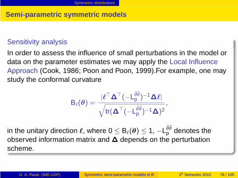
Symmetric distributions
Semi-parametric symmetric models
Sensitivity analysis
In order to assess the influence of small perturbations in the model ordata on the parameter estimates we may apply the Local InfluenceApproach (Cook, 1986; Poon and Poon, 1999).For example, one maystudy the conformal curvature
Bℓ(θ) =|ℓ⊤∆⊤(−Lθθ
p )−1∆ℓ|
√
tr(∆⊤(−Lθθp )−1∆)2
,
in the unitary direction ℓ, where 0 ≤ Bℓ(θ) ≤ 1, −Lθθp denotes the
observed information matrix and ∆ depends on the perturbationscheme.
G. A. Paula (IME-USP) Symmetric semi-parametric models in R 2o Semestre 2015 78 / 105
Boston housing data
Outline
1 Examples
2 Defining f (x)
3 Additive normal model
4 Semi-parametric normal model
5 Packages in R
6 Voltage drop data
7 Boston housing data
8 Symmetric distributions
9 Boston housing data
10 Extensions available in the library ssym
11 Comparison of snacks
12 Bibliography
G. A. Paula (IME-USP) Symmetric semi-parametric models in R 2o Semestre 2015 79 / 105
Boston housing data
Alternative models
Description
We may try to fit initially the following semi-parametric model:
LMEDVi = α+ βNOXi + f (LSTATi) + ǫi ,
G. A. Paula (IME-USP) Symmetric semi-parametric models in R 2o Semestre 2015 80 / 105
Boston housing data
Alternative models
Description
We may try to fit initially the following semi-parametric model:
LMEDVi = α+ βNOXi + f (LSTATi) + ǫi ,
where ǫiiid∼ Slash(0, φ, ζ) for i = 1, . . . , 506, with f (·) being a
continuous, smooth and nonparametric function.
G. A. Paula (IME-USP) Symmetric semi-parametric models in R 2o Semestre 2015 80 / 105
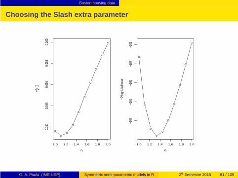
Boston housing data
Choosing the Slash extra parameter
1.0 1.2 1.4 1.6 1.8 2.0
0.04
00.
045
0.05
00.
055
0.06
0
η
Υ(η)
1.0 1.2 1.4 1.6 1.8 2.0
−107
−106
−105
−104
−103
η
−2*lo
g−Lik
eliho
od
G. A. Paula (IME-USP) Symmetric semi-parametric models in R 2o Semestre 2015 81 / 105
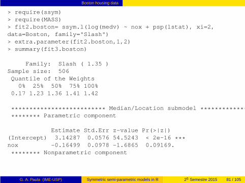
Boston housing data
> require(ssym)> require(MASS)> fit2.boston= ssym.l(log(medv) ~ nox + psp(lstat), xi=2,data=Boston, family="Slash")> extra.parameter(fit2.boston,1,2)> summary(fit3.boston)
Family: Slash ( 1.35 )Sample size: 506Quantile of the Weights0% 25% 50% 75% 100%
0.17 1.23 1.36 1.41 1.42
************************** Median/Location submodel ********************************** Parametric component
Estimate Std.Err z-value Pr(>|z|)(Intercept) 3.14287 0.0576 54.5243 < 2e-16 ***nox -0.16499 0.0978 -1.6865 0.09169.
******** Nonparametric component
G. A. Paula (IME-USP) Symmetric semi-parametric models in R 2o Semestre 2015 81 / 105
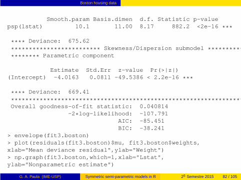
Boston housing data
Smooth.param Basis.dimen d.f. Statistic p-valuepsp(lstat) 10.1 11.00 8.17 882.2 <2e-16 ***
**** Deviance: 675.62
************************* Skewness/Dispersion submodel ******************************* Parametric component
Estimate Std.Err z-value Pr(>|z|)(Intercept) -4.0163 0.0811 -49.5386 < 2.2e-16 ***
**** Deviance: 669.41
*******************************************************************Overall goodness-of-fit statistic: 0.040814
-2*log-likelihood: -107.791AIC: -85.451BIC: -38.241
> envelope(fit3.boston)> plot(residuals(fit3.boston)$mu, fit3.boston$weights,xlab="Mean deviance residual",ylab="Weight")> np.graph(fit3.boston,which=1,xlab="Lstat",ylab="Nonparametric estimate")
G. A. Paula (IME-USP) Symmetric semi-parametric models in R 2o Semestre 2015 82 / 105
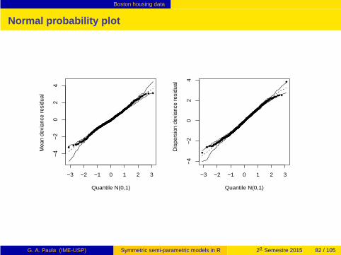
Boston housing data
Normal probability plot
−3 −2 −1 0 1 2 3
−4−2
02
4
Quantile N(0,1)
Mea
n de
vian
ce r
esid
ual
−3 −2 −1 0 1 2 3
−4−2
02
4Quantile N(0,1)
Dis
pers
ion
devi
ance
res
idua
l
G. A. Paula (IME-USP) Symmetric semi-parametric models in R 2o Semestre 2015 82 / 105
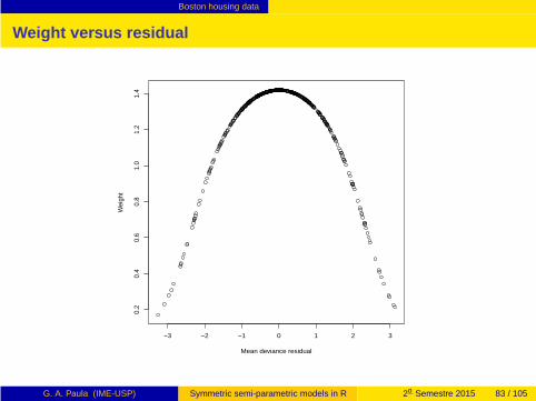
Boston housing data
Weight versus residual
−3 −2 −1 0 1 2 3
0.2
0.4
0.6
0.8
1.0
1.2
1.4
Mean deviance residual
Wei
ght
G. A. Paula (IME-USP) Symmetric semi-parametric models in R 2o Semestre 2015 83 / 105
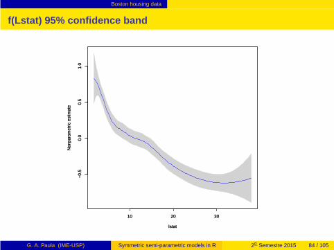
Boston housing data
f(Lstat) 95% confidence band
10 20 30
−0.5
0.0
0.5
1.0
lstat
Non
para
met
ric e
stim
ate
10 20 30
−0.5
0.0
0.5
1.0
lstat
Non
para
met
ric e
stim
ate
G. A. Paula (IME-USP) Symmetric semi-parametric models in R 2o Semestre 2015 84 / 105
Extensions available in the library ssym
Outline
1 Examples
2 Defining f (x)
3 Additive normal model
4 Semi-parametric normal model
5 Packages in R
6 Voltage drop data
7 Boston housing data
8 Symmetric distributions
9 Boston housing data
10 Extensions available in the library ssym
11 Comparison of snacks
12 Bibliography
G. A. Paula (IME-USP) Symmetric semi-parametric models in R 2o Semestre 2015 85 / 105
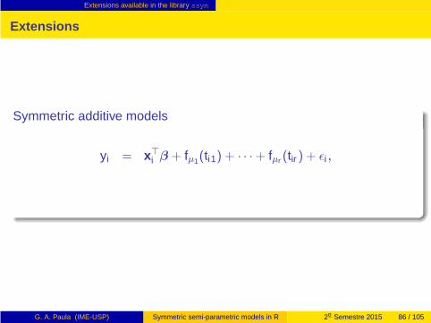
Extensions available in the library ssym
Extensions
Symmetric additive models
yi = x⊤
i β + fµ1(ti1) + · · ·+ fµr (tir ) + ǫi ,
G. A. Paula (IME-USP) Symmetric semi-parametric models in R 2o Semestre 2015 86 / 105
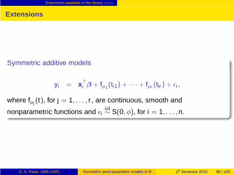
Extensions available in the library ssym
Extensions
Symmetric additive models
yi = x⊤
i β + fµ1(ti1) + · · ·+ fµr (tir ) + ǫi ,
where fµj (t), for j = 1, . . . , r , are continuous, smooth and
nonparametric functions and ǫiiid∼ S(0, φ), for i = 1, . . . , n.
G. A. Paula (IME-USP) Symmetric semi-parametric models in R 2o Semestre 2015 86 / 105
Extensions available in the library ssym
Extensions
Symmetric heteroscedastic additive models
G. A. Paula (IME-USP) Symmetric semi-parametric models in R 2o Semestre 2015 87 / 105
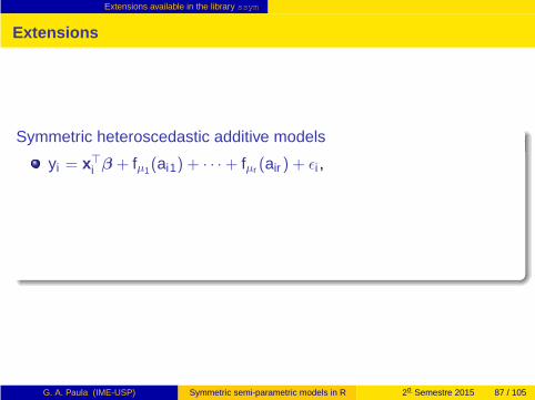
Extensions available in the library ssym
Extensions
Symmetric heteroscedastic additive models
yi = x⊤
i β + fµ1(ai1) + · · ·+ fµr (air ) + ǫi ,
G. A. Paula (IME-USP) Symmetric semi-parametric models in R 2o Semestre 2015 87 / 105

Extensions available in the library ssym
Extensions
Symmetric heteroscedastic additive models
yi = x⊤
i β + fµ1(ai1) + · · ·+ fµr (air ) + ǫi ,
ǫiind∼ S(0, φi),
G. A. Paula (IME-USP) Symmetric semi-parametric models in R 2o Semestre 2015 87 / 105
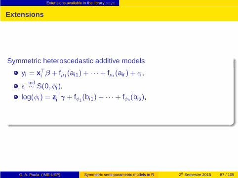
Extensions available in the library ssym
Extensions
Symmetric heteroscedastic additive models
yi = x⊤
i β + fµ1(ai1) + · · ·+ fµr (air ) + ǫi ,
ǫiind∼ S(0, φi),
log(φi) = z⊤i γ + fφ1(bi1) + · · ·+ fφs(bis),
G. A. Paula (IME-USP) Symmetric semi-parametric models in R 2o Semestre 2015 87 / 105
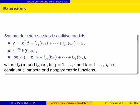
Extensions available in the library ssym
Extensions
Symmetric heteroscedastic additive models
yi = x⊤
i β + fµ1(ai1) + · · ·+ fµr (air ) + ǫi ,
ǫiind∼ S(0, φi),
log(φi) = z⊤i γ + fφ1(bi1) + · · ·+ fφs(bis),
where fµj (a) and fφk (b), for j = 1, . . . , r and k = 1, . . . , s, arecontinuous, smooth and nonparametric functions.
G. A. Paula (IME-USP) Symmetric semi-parametric models in R 2o Semestre 2015 87 / 105
Extensions available in the library ssym
Extensions
Symmetric nonlinear additive models
G. A. Paula (IME-USP) Symmetric semi-parametric models in R 2o Semestre 2015 88 / 105
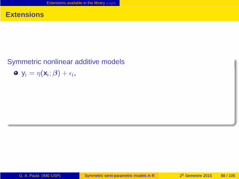
Extensions available in the library ssym
Extensions
Symmetric nonlinear additive models
yi = η(x i ;β) + ǫi ,
G. A. Paula (IME-USP) Symmetric semi-parametric models in R 2o Semestre 2015 88 / 105

Extensions available in the library ssym
Extensions
Symmetric nonlinear additive models
yi = η(x i ;β) + ǫi ,
ǫiind∼ S(0, φi),
G. A. Paula (IME-USP) Symmetric semi-parametric models in R 2o Semestre 2015 88 / 105
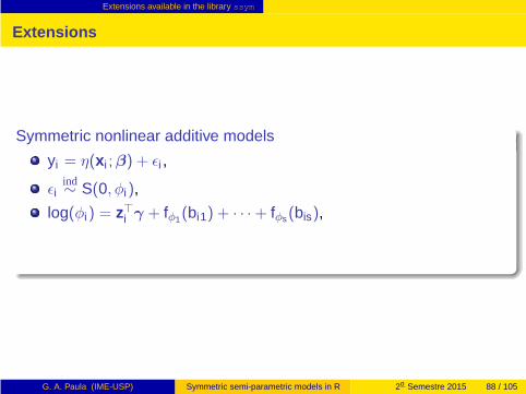
Extensions available in the library ssym
Extensions
Symmetric nonlinear additive models
yi = η(x i ;β) + ǫi ,
ǫiind∼ S(0, φi),
log(φi) = z⊤i γ + fφ1(bi1) + · · ·+ fφs(bis),
G. A. Paula (IME-USP) Symmetric semi-parametric models in R 2o Semestre 2015 88 / 105
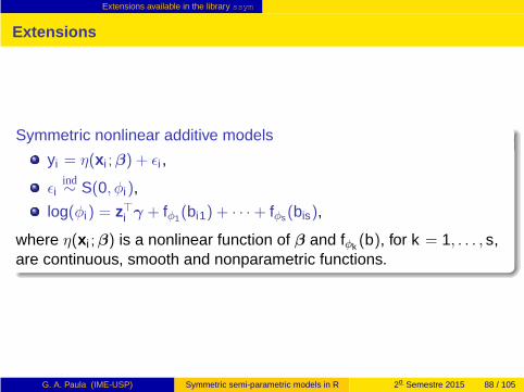
Extensions available in the library ssym
Extensions
Symmetric nonlinear additive models
yi = η(x i ;β) + ǫi ,
ǫiind∼ S(0, φi),
log(φi) = z⊤i γ + fφ1(bi1) + · · ·+ fφs(bis),
where η(x i ;β) is a nonlinear function of β and fφk (b), for k = 1, . . . , s,are continuous, smooth and nonparametric functions.
G. A. Paula (IME-USP) Symmetric semi-parametric models in R 2o Semestre 2015 88 / 105
Comparison of snacks
Outline
1 Examples
2 Defining f (x)
3 Additive normal model
4 Semi-parametric normal model
5 Packages in R
6 Voltage drop data
7 Boston housing data
8 Symmetric distributions
9 Boston housing data
10 Extensions available in the library ssym
11 Comparison of snacks
12 Bibliography
G. A. Paula (IME-USP) Symmetric semi-parametric models in R 2o Semestre 2015 89 / 105
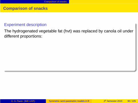
Comparison of snacks
Comparison of snacks
Experiment description
The hydrogenated vegetable fat (hvt) was replaced by canola oil underdifferent proportions:
G. A. Paula (IME-USP) Symmetric semi-parametric models in R 2o Semestre 2015 90 / 105

Comparison of snacks
Comparison of snacks
Experiment description
The hydrogenated vegetable fat (hvt) was replaced by canola oil underdifferent proportions:
A: 22% hvf, 0% canola oil
G. A. Paula (IME-USP) Symmetric semi-parametric models in R 2o Semestre 2015 90 / 105
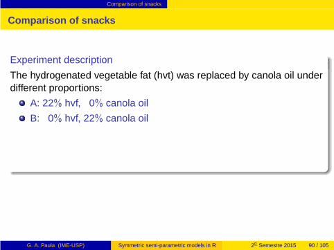
Comparison of snacks
Comparison of snacks
Experiment description
The hydrogenated vegetable fat (hvt) was replaced by canola oil underdifferent proportions:
A: 22% hvf, 0% canola oil
B: 0% hvf, 22% canola oil
G. A. Paula (IME-USP) Symmetric semi-parametric models in R 2o Semestre 2015 90 / 105
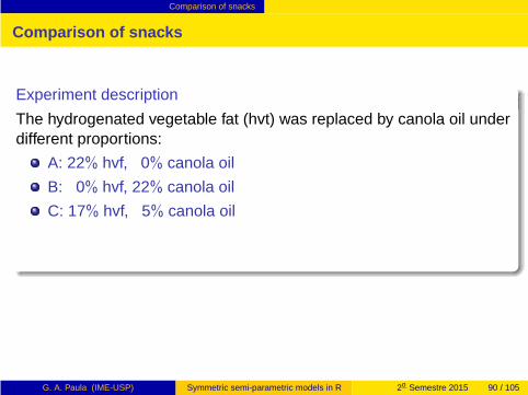
Comparison of snacks
Comparison of snacks
Experiment description
The hydrogenated vegetable fat (hvt) was replaced by canola oil underdifferent proportions:
A: 22% hvf, 0% canola oil
B: 0% hvf, 22% canola oil
C: 17% hvf, 5% canola oil
G. A. Paula (IME-USP) Symmetric semi-parametric models in R 2o Semestre 2015 90 / 105
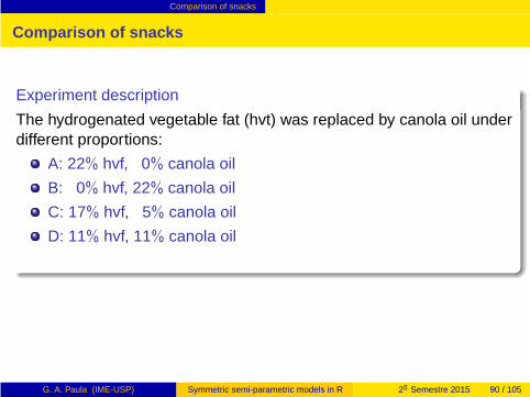
Comparison of snacks
Comparison of snacks
Experiment description
The hydrogenated vegetable fat (hvt) was replaced by canola oil underdifferent proportions:
A: 22% hvf, 0% canola oil
B: 0% hvf, 22% canola oil
C: 17% hvf, 5% canola oil
D: 11% hvf, 11% canola oil
E: 5% hvf, 17% canola oil.
G. A. Paula (IME-USP) Symmetric semi-parametric models in R 2o Semestre 2015 90 / 105
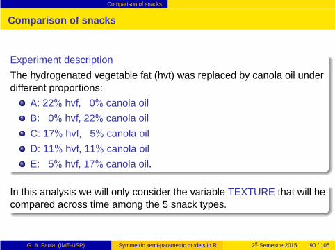
Comparison of snacks
Comparison of snacks
Experiment description
The hydrogenated vegetable fat (hvt) was replaced by canola oil underdifferent proportions:
A: 22% hvf, 0% canola oil
B: 0% hvf, 22% canola oil
C: 17% hvf, 5% canola oil
D: 11% hvf, 11% canola oil
E: 5% hvf, 17% canola oil.
In this analysis we will only consider the variable TEXTURE that will becompared across time among the 5 snack types.
G. A. Paula (IME-USP) Symmetric semi-parametric models in R 2o Semestre 2015 90 / 105
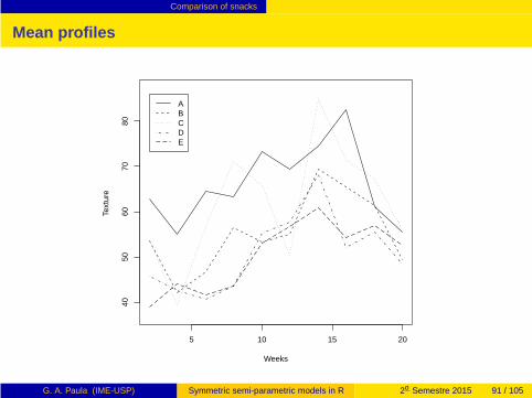
Comparison of snacks
Mean profiles
5 10 15 20
4050
6070
80
Weeks
Text
ure
ABCDE
G. A. Paula (IME-USP) Symmetric semi-parametric models in R 2o Semestre 2015 91 / 105
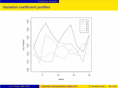
Comparison of snacks
Variation coefficient profiles
5 10 15 20
0.05
0.10
0.15
0.20
0.25
0.30
0.35
Weeks
VC
of T
extu
reABCDE
G. A. Paula (IME-USP) Symmetric semi-parametric models in R 2o Semestre 2015 92 / 105
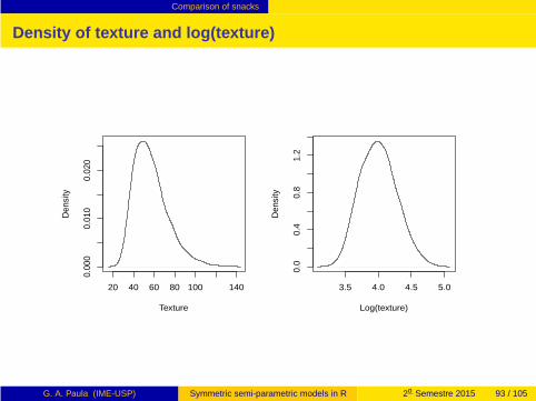
Comparison of snacks
Density of texture and log(texture)
20 40 60 80 100 140
0.00
00.
010
0.02
0
Texture
Den
sity
3.5 4.0 4.5 5.00.
00.
40.
81.
2Log(texture)
Den
sity
G. A. Paula (IME-USP) Symmetric semi-parametric models in R 2o Semestre 2015 93 / 105
Comparison of snacks
Alternative models
Description
We will consider the following semi-parametric model:
G. A. Paula (IME-USP) Symmetric semi-parametric models in R 2o Semestre 2015 94 / 105
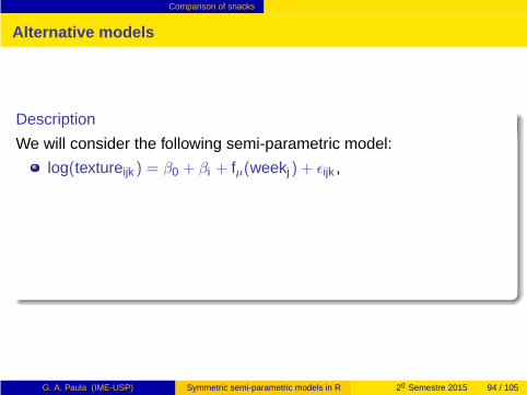
Comparison of snacks
Alternative models
Description
We will consider the following semi-parametric model:
log(textureijk ) = β0 + βi + fµ(weekj) + ǫijk ,
G. A. Paula (IME-USP) Symmetric semi-parametric models in R 2o Semestre 2015 94 / 105
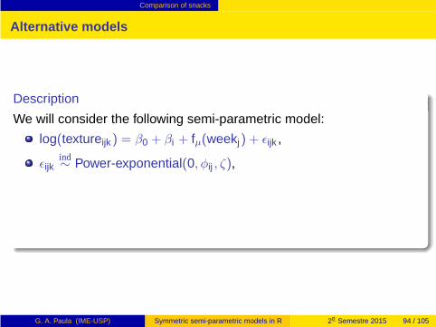
Comparison of snacks
Alternative models
Description
We will consider the following semi-parametric model:
log(textureijk ) = β0 + βi + fµ(weekj) + ǫijk ,
ǫijkind∼ Power-exponential(0, φij , ζ),
G. A. Paula (IME-USP) Symmetric semi-parametric models in R 2o Semestre 2015 94 / 105
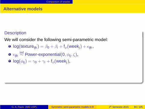
Comparison of snacks
Alternative models
Description
We will consider the following semi-parametric model:
log(textureijk ) = β0 + βi + fµ(weekj) + ǫijk ,
ǫijkind∼ Power-exponential(0, φij , ζ),
log(φij) = γ0 + γi + fφ(weekj),
for i = 1(A), 2(B), 3(C), 4(D), 5(E), j = 2, 4, . . . , 20 and k = 1, . . . , 15,β0 + βi (β1 = 0) and γ0 + γi (γ1 = 0) denote the snack effects whereasfµ(·) and fφ(·) are continuous, smooth and nonparametric functions.
G. A. Paula (IME-USP) Symmetric semi-parametric models in R 2o Semestre 2015 94 / 105

Comparison of snacks
Choosing the power exponential extra parameter
0.0 0.2 0.4 0.6
0.03
0.04
0.05
0.06
η
Υ(η)
0.0 0.2 0.4 0.6
−235
−230
−225
−220
−215
−210
η
−2*lo
g−Lik
eliho
od
G. A. Paula (IME-USP) Symmetric semi-parametric models in R 2o Semestre 2015 95 / 105
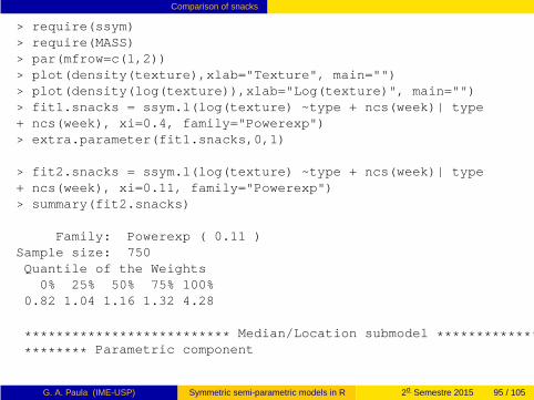
Comparison of snacks
> require(ssym)> require(MASS)> par(mfrow=c(1,2))> plot(density(texture),xlab="Texture", main="")> plot(density(log(texture)),xlab="Log(texture)", main="")> fit1.snacks = ssym.l(log(texture) ~type + ncs(week)| type+ ncs(week), xi=0.4, family="Powerexp")> extra.parameter(fit1.snacks,0,1)
> fit2.snacks = ssym.l(log(texture) ~type + ncs(week)| type+ ncs(week), xi=0.11, family="Powerexp")> summary(fit2.snacks)
Family: Powerexp ( 0.11 )Sample size: 750Quantile of the Weights0% 25% 50% 75% 100%
0.82 1.04 1.16 1.32 4.28
************************** Median/Location submodel ********************************** Parametric component
G. A. Paula (IME-USP) Symmetric semi-parametric models in R 2o Semestre 2015 95 / 105
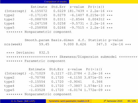
Comparison of snacks
Estimate Std.Err z-value Pr(>|z|)(Intercept) 4.155072 0.0229 181.7439 < 2.2e-16 ***type2 -0.171145 0.0279 -6.1407 8.215e-10 ***type3 -0.088709 0.0311 -2.8544 0.004312 **type4 -0.247158 0.0258 -9.5731 < 2.2e-16 ***type5 -0.258958 0.0266 -9.7515 < 2.2e-16 *********** Nonparametric component
Smooth.param Basis.dimen d.f. Statistic p-valuencs(week) 59.45 9.000 8.626 347.3 <2e-16 ***
**** Deviance: 832.5
************************* Skewness/Dispersion submodel ******************************* Parametric component
Estimate Std.Err z-value Pr(>|z|)(Intercept) -2.71029 0.1217 -22.2784 < 2.2e-16 ***type2 -0.70798 0.1720 -4.1150 3.871e-05 ***type3 -0.15554 0.1720 -0.9041 0.366type4 -1.26983 0.1720 -7.3807 1.574e-13 ***type5 -1.03528 0.1720 -6.0174 1.772e-09 *********** Nonparametric component
G. A. Paula (IME-USP) Symmetric semi-parametric models in R 2o Semestre 2015 95 / 105
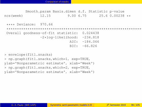
Comparison of snacks
Smooth.param Basis.dimen d.f. Statistic p-valuencs(week) 12.15 9.00 6.75 25.6 0.00238 **
**** Deviance: 970.64
*******************************************************************Overall goodness-of-fit statistic: 0.024438
-2*log-likelihood: -234.818AIC: -184.066BIC: -66.826
> envelope(fit1.snacks)> np.graph(fit1.snacks,which=1, exp=TRUE,ylab="Nonparametric estimate", xlab="Week")> np.graph(fit1.snacks,which=2, exp=TRUE,ylab="Nonparametric estimate", xlab="Week")
G. A. Paula (IME-USP) Symmetric semi-parametric models in R 2o Semestre 2015 96 / 105

Comparison of snacks
Normal probability plot
−3 −2 −1 0 1 2 3
−20
24
Quantile N(0,1)
Mea
n de
vian
ce r
esid
ual
−3 −2 −1 0 1 2 3
−4−2
02
4Quantile N(0,1)
DeD
ispe
rsio
n de
vian
ce r
esid
ual
G. A. Paula (IME-USP) Symmetric semi-parametric models in R 2o Semestre 2015 96 / 105
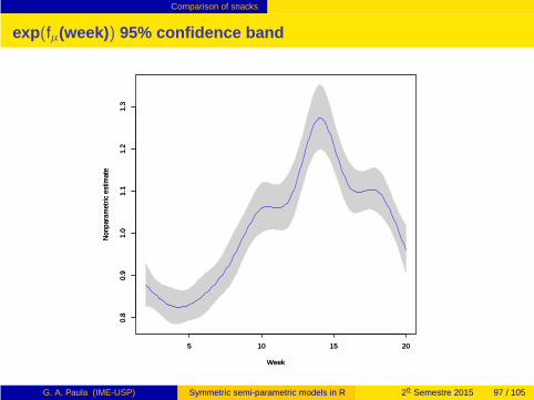
Comparison of snacks
exp(fµ(week)) 95% confidence band
5 10 15 20
0.8
0.9
1.0
1.1
1.2
1.3
Week
Non
para
met
ric e
stim
ate
5 10 15 20
0.8
0.9
1.0
1.1
1.2
1.3
Week
Non
para
met
ric e
stim
ate
G. A. Paula (IME-USP) Symmetric semi-parametric models in R 2o Semestre 2015 97 / 105
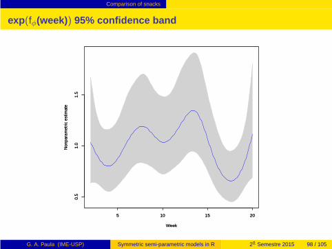
Comparison of snacks
exp(fφ(week)) 95% confidence band
5 10 15 20
0.5
1.0
1.5
Week
Non
para
met
ric e
stim
ate
5 10 15 20
0.5
1.0
1.5
Week
Non
para
met
ric e
stim
ate
G. A. Paula (IME-USP) Symmetric semi-parametric models in R 2o Semestre 2015 98 / 105
Bibliography
Outline
1 Examples
2 Defining f (x)
3 Additive normal model
4 Semi-parametric normal model
5 Packages in R
6 Voltage drop data
7 Boston housing data
8 Symmetric distributions
9 Boston housing data
10 Extensions available in the library ssym
11 Comparison of snacks
12 Bibliography
G. A. Paula (IME-USP) Symmetric semi-parametric models in R 2o Semestre 2015 99 / 105

Bibliography
References
References
G. A. Paula (IME-USP) Symmetric semi-parametric models in R 2o Semestre 2015 100 / 105
Bibliography
References
References
Barros M, Paula GA and Leiva, V (2008). A new class of survivalregression models with heavy-tailed errors: robustness anddiagnostics. Lifetime Data Analysis, 14, 316-332.
G. A. Paula (IME-USP) Symmetric semi-parametric models in R 2o Semestre 2015 100 / 105
Bibliography
References
References
Barros M, Paula GA and Leiva, V (2008). A new class of survivalregression models with heavy-tailed errors: robustness anddiagnostics. Lifetime Data Analysis, 14, 316-332.
Belsley DA, Kuh E and Welsch RE (1980). RegressionDiagnostics. Identifying Influential Data and Sources ofCollinearity. Wiley, New York.
Cook RD (1986). Assessment local influence (with discussion).Journal of the Royal Statistical Society, Series B, 48, 133-169.
G. A. Paula (IME-USP) Symmetric semi-parametric models in R 2o Semestre 2015 100 / 105

Bibliography
References
References
Barros M, Paula GA and Leiva, V (2008). A new class of survivalregression models with heavy-tailed errors: robustness anddiagnostics. Lifetime Data Analysis, 14, 316-332.
Belsley DA, Kuh E and Welsch RE (1980). RegressionDiagnostics. Identifying Influential Data and Sources ofCollinearity. Wiley, New York.
Cook RD (1986). Assessment local influence (with discussion).Journal of the Royal Statistical Society, Series B, 48, 133-169.
Cysneiros FJA, Paula GA and Galea M (2005). ModelosSimétricos Aplicados. Livro Texto de Minicurso da 9a Escola deModelos de Regressão, Associação Brasileira de Estatística, SP,Brasil.
G. A. Paula (IME-USP) Symmetric semi-parametric models in R 2o Semestre 2015 100 / 105

Bibliography
References
References
G. A. Paula (IME-USP) Symmetric semi-parametric models in R 2o Semestre 2015 101 / 105
Bibliography
References
References
De Boor C (1978). A Practical Guide to Splines. AppliedMathematical Sciences. Springer-Verlag, New York.
G. A. Paula (IME-USP) Symmetric semi-parametric models in R 2o Semestre 2015 101 / 105
Bibliography
References
References
De Boor C (1978). A Practical Guide to Splines. AppliedMathematical Sciences. Springer-Verlag, New York.
Díaz-García JA and Leiva V (2005). A new family of lifedistributions based on elliptically contoured distributions. Journalof Statistical Planning & Inference, 128, 445-457.
Fang K, Kotz S and Ng K (1990). Symmetric Multivariate andRelated Distribution. Chapman and Hall, London.
Gómez E, Gómez-Villegas MA and Marín JM (1998). Amultivariate generalization of the power exponential family ofdistributions. Communications in Statistics - Theory and Methods27, 589-600.
G. A. Paula (IME-USP) Symmetric semi-parametric models in R 2o Semestre 2015 101 / 105

Bibliography
References
References
G. A. Paula (IME-USP) Symmetric semi-parametric models in R 2o Semestre 2015 102 / 105
Bibliography
References
References
Hastie TJ and Tibshirani RJ (1990). Generalized Additive Models.Chapman and Hall, London.
G. A. Paula (IME-USP) Symmetric semi-parametric models in R 2o Semestre 2015 102 / 105

Bibliography
References
References
Hastie TJ and Tibshirani RJ (1990). Generalized Additive Models.Chapman and Hall, London.
Ibacache-Pulgar G, Paula GA and Cysneiros, FJA (2013).Semiparametric additive models under symmetric distributions.TEST, 22, 103-121.
G. A. Paula (IME-USP) Symmetric semi-parametric models in R 2o Semestre 2015 102 / 105
Bibliography
References
References
Hastie TJ and Tibshirani RJ (1990). Generalized Additive Models.Chapman and Hall, London.
Ibacache-Pulgar G, Paula GA and Cysneiros, FJA (2013).Semiparametric additive models under symmetric distributions.TEST, 22, 103-121.
Kafadar K (1988). Slash Distribution, Encyclopedia of StatisticalSciences. Johnson, N.L., Kotz, S., Read, C., Eds., Vol. 8,510-511. Wiley, New York.
Osorio F, Paula GA and Galea M (2007). Assessment of localinfluence in elliptical linear models with longitudidnal structure.Computational Statistics and Data Analysis, 51, 4354-4368.
G. A. Paula (IME-USP) Symmetric semi-parametric models in R 2o Semestre 2015 102 / 105

Bibliography
References
References
G. A. Paula (IME-USP) Symmetric semi-parametric models in R 2o Semestre 2015 103 / 105
Bibliography
References
References
Lange KL, Little RJA and Taylor JMG (1989). Robust statisticalmodeling using the t distribution. Journal of the AmericanStatistical Association, 84, 881-896.
G. A. Paula (IME-USP) Symmetric semi-parametric models in R 2o Semestre 2015 103 / 105
Bibliography
References
References
Lange KL, Little RJA and Taylor JMG (1989). Robust statisticalmodeling using the t distribution. Journal of the AmericanStatistical Association, 84, 881-896.
Little RJA (1988). Robust estimation of the mean and covariancematrix from data with missing values. Applied Statistics, 37, 23-38.
Leiva V, Barros M, Paula GA and Galea M (2007). Influencediagnostics in log-BirnbaumUSaunders regression models withcensored data. Computational Statistics and Data Analysis, 51,5694-5707.
Montgomery DC, Peck EA and Vining GG (2001). Introduction toLinear Regression Analysis, 3rd Edition. Wiley, New York.
G. A. Paula (IME-USP) Symmetric semi-parametric models in R 2o Semestre 2015 103 / 105

Bibliography
References
References
G. A. Paula (IME-USP) Symmetric semi-parametric models in R 2o Semestre 2015 104 / 105
Bibliography
References
References
Poon WY and Poon YS (1999). Conformal normal curvature andassessment of local influence. Journal of the Royal StatisticalSociety, Series B, 61, 51-61.
G. A. Paula (IME-USP) Symmetric semi-parametric models in R 2o Semestre 2015 104 / 105
Bibliography
References
References
Poon WY and Poon YS (1999). Conformal normal curvature andassessment of local influence. Journal of the Royal StatisticalSociety, Series B, 61, 51-61.
Rieck JR and Nedelman JR (1991). A log-linear model for theBirnbaum-Saunders distribution. Technometrics, 33, 51-60.
G. A. Paula (IME-USP) Symmetric semi-parametric models in R 2o Semestre 2015 104 / 105
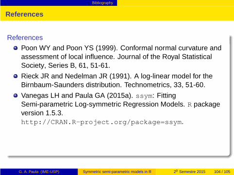
Bibliography
References
References
Poon WY and Poon YS (1999). Conformal normal curvature andassessment of local influence. Journal of the Royal StatisticalSociety, Series B, 61, 51-61.
Rieck JR and Nedelman JR (1991). A log-linear model for theBirnbaum-Saunders distribution. Technometrics, 33, 51-60.
Vanegas LH and Paula GA (2015a). ssym: FittingSemi-parametric Log-symmetric Regression Models. R packageversion 1.5.3.http://CRAN.R-project.org/package=ssym.
G. A. Paula (IME-USP) Symmetric semi-parametric models in R 2o Semestre 2015 104 / 105
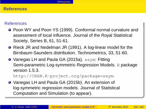
Bibliography
References
References
Poon WY and Poon YS (1999). Conformal normal curvature andassessment of local influence. Journal of the Royal StatisticalSociety, Series B, 61, 51-61.
Rieck JR and Nedelman JR (1991). A log-linear model for theBirnbaum-Saunders distribution. Technometrics, 33, 51-60.
Vanegas LH and Paula GA (2015a). ssym: FittingSemi-parametric Log-symmetric Regression Models. R packageversion 1.5.3.http://CRAN.R-project.org/package=ssym.
Vanegas LH and Paula GA (2015b). An extension oflog-symmetric regression models. Journal of StatisticalComputation and Simulation (to appear).
G. A. Paula (IME-USP) Symmetric semi-parametric models in R 2o Semestre 2015 104 / 105

Bibliography
References
References
G. A. Paula (IME-USP) Symmetric semi-parametric models in R 2o Semestre 2015 105 / 105
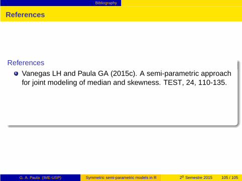
Bibliography
References
References
Vanegas LH and Paula GA (2015c). A semi-parametric approachfor joint modeling of median and skewness. TEST, 24, 110-135.
G. A. Paula (IME-USP) Symmetric semi-parametric models in R 2o Semestre 2015 105 / 105
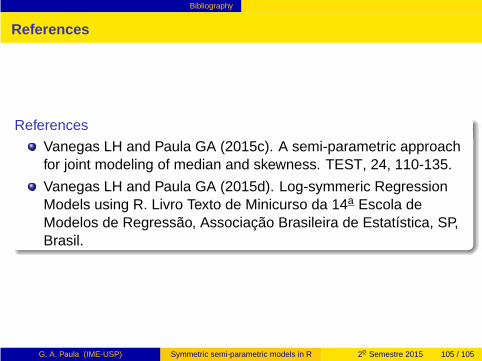
Bibliography
References
References
Vanegas LH and Paula GA (2015c). A semi-parametric approachfor joint modeling of median and skewness. TEST, 24, 110-135.
Vanegas LH and Paula GA (2015d). Log-symmeric RegressionModels using R. Livro Texto de Minicurso da 14a Escola deModelos de Regressão, Associação Brasileira de Estatística, SP,Brasil.
G. A. Paula (IME-USP) Symmetric semi-parametric models in R 2o Semestre 2015 105 / 105