A note on semi-parametric estimatorsYen-Chi Chen

University of WashingtonMay 5, 2020

Contents

1 Influence function and score vector 3

2 Efficient influence function 4

2.1 Constructing efficient influence function using score vectors . . . . . . . . . . . . . . . . . 6

3 Semiparametric estimator 6

3.1 Parametric submodels . . . . . . . . . . . . . . . . . . . . . . . . . . . . . . . . . . . . . . 7

3.2 Generalizing RAL estimators to a semi-parametric model . . . . . . . . . . . . . . . . . . . 8

3.3 Semi-paramteric nuisance tangent space . . . . . . . . . . . . . . . . . . . . . . . . . . . . 9

4 Finding efficient estimators: tangent space approach 10

4.1 Conditional factorization . . . . . . . . . . . . . . . . . . . . . . . . . . . . . . . . . . . . 11

4.2 Example: restricted moment model . . . . . . . . . . . . . . . . . . . . . . . . . . . . . . . 14

4.3 Example: Cox Model . . . . . . . . . . . . . . . . . . . . . . . . . . . . . . . . . . . . . . 17

5 Finding efficient estimators: geometric approach 21

5.1 Differentiation in quadratic mean . . . . . . . . . . . . . . . . . . . . . . . . . . . . . . . . 21

5.2 Geometry of influence functions . . . . . . . . . . . . . . . . . . . . . . . . . . . . . . . . 22

5.3 Example: simple missing at random problem . . . . . . . . . . . . . . . . . . . . . . . . . 24

5.3.1 Method 1: inverse probability weighting . . . . . . . . . . . . . . . . . . . . . . . . 26

5.3.2 Method 2: regression adjustment (g-computation) . . . . . . . . . . . . . . . . . . . 28

5.4 More about DQM . . . . . . . . . . . . . . . . . . . . . . . . . . . . . . . . . . . . . . . . 31

6 Finding efficient estimators: conditional expectation 33

6.1 Finding a computable influence function and efficient estimator . . . . . . . . . . . . . . . . 34

6.2 Example: current status model . . . . . . . . . . . . . . . . . . . . . . . . . . . . . . . . . 34

1

Semi-parametric model offers a set of flexible tools in data analysis that has a fast convergence rate. Thehigh-level idea is that we want to estimate a parameter of interest that is a finite dimensional object but wedo not place any parametric constraint on the full model.

To see why this is interesting, consider density estimation problem where we observe X1, · · · ,Xn ∼ p. Toestimate the underlying PDF p, we may use kernel density estimator, histogram, basis approach, ...etc.However, we cannot estimate p in a fast rate; under usual assumption (known as the Holder condition, whichis similar to the condition that p is bounded twice-differentiable), the best rate (in terms of minimaxity) thatwe can achieve is supx |p(x)− p(x)| = OP(n−

24+d ), which is clearly slower than the usual parametric rate

OP(n−12 ). Note that d is the dimension of X . On the other hand, if we assume that the distribution is a normal

distribution, we can estimate the mean and variance at rate OP(n−12 ) so we can achieve that convergence rate

supx |p(x)− p(x)|= OP(n−12 ).

The power of semi-parametric estimator is that there are cases where we can achieve a parametric rate with-out assuming that the entire model is a parametric model. For instance, consider estimating the populationmean µ = E(X) where X ∈ Rd . Clearly, the sample mean

µn =1n

n

∑i=1

Xi

is a√

n-consistent estimator. But note that the consistency of µn does not require any parametric assumptionon the entire distribution. For another example, consider the linear regression problem where we model(assuming no intercept)

Yi = βT Xi + εi.

The least square estimator βn from minimizing

Rn(β) =n

∑i=1

(Yi−βT Xi)

2

also converges to the true parameter (assuming that the linear model is correct) even if we do not specify thedistribution of X and ε|X to be parametric models.

In this note, we give a gentle introduction of semi-parametric estimators. We start with a properties of aparametric model that are relevant to semi-parametric models and then discuss how to construct a semi-parametric estimator. In particular, we will discuss three approaches–the first one is based on characterizingthe tangent space, the second one is based on the geometry of influence function, and the third one is basedon conditional expectation.

The first part of the note is mostly based on Chapter 3 and 4 of the following book:

Tsiatis, A. (2007). Semiparametric theory and missing data. Springer Science & BusinessMedia.

The later part of the note will be from Chapter 25 of the following book:

Van der Vaart, A. W. (2000). Asymptotic statistics (Vol. 3). Cambridge university press.

2

1 Influence function and score vector

Consider a simple parametric model where we observe

X1, · · · ,Xn ∼ p(x;θ0),

where θ0 is the underlying parameter. Assume that we can decompose the parameter θ0 = (β0,η0) such thatour primary interest is β ∈ Rq. In this case, η ∈ Rr will be called a nuisance parameter.

An estimator βn of β0 is called asymptotically linear with influence function ψ(x) if

√n(βn−β0) =

1√n

n

∑i=1

ψ(Xi)+oP(1)

and E(ψ(X)) = 0 and E(ψ(X)ψ(X)T ) is finite and non-singular. Note that here we did not specify how toconstruct βn; there is often many asymptotically linear estimator of the same parameter of interest (eachcorresponds to a different influence function).

Since we are using a parametric model, the score vector is often of a lot of interest. Let

Sθ(x;θ) =∂

∂θlog p(x;θ) ∈ Rq+r

Sβ(x;θ) =∂

∂βlog p(x;θ) ∈ Rq

Sη(x;θ) =∂

∂ηlog p(x;θ) ∈ Rr

be the score vectors.

From the theory of MLE (maximum likelihood estimator), we know that the score vector often plays akey role in the construction of an estimator. So one may be wondering how will the score vector and theinfluence function related. The following theorem provides a powerful link between them.

Theorem 1 (Theorem 3.2 of Tsiatis 2007) If βn is a regular1 estimator, then

E(ψ(X)STβ(X ;θ0)) = Iq×q, E(ψ(X)ST

η(X ;θ0)) = 0q×r, (1)

where Iq×q is the q×q identity matrix.

The power of Theorem 1 is that it works for any regular asymptotic normal (RAL) estimator! It does notrequire any specific construction of the estimator. For instance, if we use the method of moments to constructβn, Theorem 1 will apply.

Equation (1) is not just a necessarily condition for an RAL estimator. If we have a function ψ that satisfiesequation (1), we can construct an RAL estimator with influence function being ψ.

1in general, we are often using a regular estimator; the precise definition can be found in Definition 1 of Tsiatis 2007.

3

Theorem 2 (Converting influence function into an estimator) Let ψ(X) be a function satisfying equation(1). Assume that for each β, we have an estimator ηn(β) such that

√n‖ηn(β)− η0‖max is bounded in

probabiiltiy. Define m(X ;β,η) = ψ(X)−EX∼p(·;β,η)(ψ(X)) and let β be the solution ofn

∑i=1

m(Xi;β, ηn(β)) = 0.

Then βn will be an RAL estimator with influence function ψ(X).

The proof of this theorem can be found in page 39-40 of Tsiatis (2007).

Theorem 2 provides a procedure to convert a function satisfying equation (1) into an estimator with thatfunction being an influence function. With Theorem 1, we can informally say that the set/space

G =

ψ : E(ψ(X)STβ(X ;θ0)) = Iq×q, E(ψ(X)ST

η(X ;θ0)) = 0q×r

characterizes all RAL estimators. In particular, the second equality E(ψ(X)ST

η(X ;θ0)) = 0q×r can be re-written as

Π(ψ(X)|Fη) = 0,

where Fη is the nuisance tangent space (will be introduced later).

2 Efficient influence function

Now we have learned that there can be many RAL estimators. One may be wondering: what is the optimalRAL estimator? how do we construct the optimal RAL estimator? Here the best is often referred to theestimator with the smallest variance (since an RAL estimator is asymptotically unbiased). To answer thesequestions, we go back to conditions in equation (1).

The conditionE(ψ(X)ST

η(X ;θ0)) = 0q×r

is particularly interesting since the conditional mean being 0 is often related to orthogonal projection. Tofurther investigate this, we introduce the nuisance tangent space

Fη = BSη(x;θ0) : B ∈ Rq×r.

Namely, Fη is a collection of functions that is along the direction of the score vector Sη(x;θ0) and projectedinto the space of β (the effect of the coefficient matrix B). Similarly, we define

Fβ = BSβ(x;θ0) : B ∈ Rq×qF = BSθ(x;θ0) : B ∈ Rq×(q+r)

and we can write F = Fβ⊕Fη with the notation

F1⊕F2 = f1 + f2 : f1 ∈ F1, f2 ∈ F2.

F is called the tangent space and it has a very interesting property–it characterizes the space of all RALestimators!

4

Theorem 3 (Theorem 3.4 of Tsiatis 2007) Let ψ1,ψ2 be any two influence functions of RAL estimators ofβ0. Then

ψ1−ψ2 ∈ F ⊥.

Namely,E((ψ1(X)−ψ2(X))ST

θ (X ;θ0)) = 0q×(q+r).

In other words, Theorem 3 shows that if we can find an influence function ψ, then we can find all other influ-ence functions by adding a term from the orthogonal space of the tangent space. Together with Theorem 1and 2, this implies that we have a way to characterize all RAL estimators!

This is a powerful result for our purposes because the search of the optimal RAL estimator can be doneby examining the tangent space if we have obtained an influence function. The influence function thatcorresponds to the RAL estimator with the smallest variance is called efficient influence function.

Theorem 3 implies that we will be working on estimator of the form:

ψ(x) = ψ0(x)+g(x), g ∈ Fη,

where ψ0 is a given function. Thus, the variance of the estimator constructed by ψ will be written as

Var(ψ(X)) = Var(ψ0(X)+g(X)).

This quantity is not easy to analyze since it is a covariance matrix and ψ0(X) and g(X) may be highlycorrelated. However, here is an interesting note from the Pythagorean theorem. For a function h(x) ∈ Rq,denote its projection onto a subspace G as Π(h(x)|G). Then

Var(h(X)) = Var(Π(h(X)|G))+Var(h(X)−Π(h(X)|G))≥ Var(Π(h(X)|G)).

Note that for matrices A≥ B, this means that A−B is positive definite. From the above inequality, one caneasily deduce the following result:

Theorem 4 (Theorem 3.5 of Tsiatis 2007) Let ψ0 be any influence function satisfying equation (1). Thethe efficient influence function can be constructed using

ψeff(X) = ψ0(X)−Π(ψ0(X)|F ⊥) = Π(ψ0(X)|F ).

In general, obtaining a projection is not easy. But here the space we are considering is a linear space sothe projection can be easily defined. Take the tangent space as an example. For a function h(x) ∈ Rq, itsprojection onto F is

Π(h(x)|F ) = E(h(X)STθ (X ;θ0))[E(Sθ(X ;θ0)ST

θ (X ;θ0))]−1Sθ(x;θ0).

Thus, for any influence function ψ0 satisfying equation (1),

ψeff(X) = E(ψ0(X)STθ (X ;θ0))[E(Sθ(X ;θ0)ST

θ (X ;θ0))]−1Sθ(x;θ0).

5

2.1 Constructing efficient influence function using score vectors

The above procedure is useful when we have an influence function already. In practice, we may not have aninfluence function so how to construct an efficient influence function is unclear. Here is a simple approachthat based on the score vectors.

We define the efficient score vector as

Seff(X ;θ0) = Π(Sβ(X ;θ0)|F ⊥η )

= Sβ(X ;θ0)−Π(Sβ(X ;θ0)|Fη)

= Sβ(X ;θ0)−E(Sβ(X ;θ0)STη(X ;θ0))[E(Sη(X ;θ0)ST

η(X ;θ0))]−1Sη(X ;θ0)

(2)

By construction, Seff(X ;θ0) satisfies E(Seff(X ;θ0)STη(X ;θ0)) = 0q×r so it satisfies the second equality in

equation (1).

To ensure the first equality in equation (1), using the fact that

E(Seff(X ;θ0)STβ(X ;θ0)) = E(Seff(X ;θ0)ST

eff(X ;θ0)),

we construct the influence function as

ψscore(X) = [E(Seff(X ;θ0)STeff(X ;θ0))]

−1Seff(X ;θ0).

One can verify that ψscore(X) satisfies equation (1).

Because Seff(X ;θ0) ∈ Fβ ⊕Fη = F , it is easy to see that Π(ψscore(X)|F ) = ψscore(X) so ψscore(X) =ψeff(X)! Moreover, the minimal variance (known as the efficiency bound) will be

Var(ψeff(X)) = [E(Seff(X ;θ0)STeff(X ;θ0))]

−1.

3 Semiparametric estimator

The above result is very powerful–we know how to construct the optimal (efficient) estimator. However, itis also restrictive in the sense that it requires a parametric model. In many scenarios, we are interested inβ ∈ Rq that is finite dimensional but we do not want to limit ourselves to a parametric approach of η. Herewe will generalize the techniques in the previous section so that they work even if the nuisance parameter η

may be infinite dimensional. In this case, the problem is called the semiparametric estimation problem.

Here are two common examples.

• Moment restricted model. Consider a regression problem where

Yi = µ(Xi;β)+ εi, E(εi|Xi) = 0,

where µ is a known function (for instance, linear regression requires µ(Xi;β) = α+XTi β). The param-

eter of interest is β. The nuisance parameter is the PDF of ε|X = x and the PDF of X .

6

• Proportional hazard model. The proportional hazard model is a very popular approach in survivalanalysis. The data consists of (X1,T1), · · · ,(Xn,Tn) and let F(t|x) be the CDF of T given X = x. Thesurvival function S(t|x) = 1−F(t|x). The hazard function is defined as λ(t|x) = − d

dt logS(t|x). Theproportional hazard model assumes that

λ(t|x;β) = λ0(t)exp(βT x).

Again, β is the parameter of interest and λ0, the baseline hazard function, is the nuisance parameter.

In the above problems, the nuisance parameters are functions so they are infinite dimensional objects. Theamazing part of the semiparametric inference is that we can still obtain a

√n-rate estimator for β!

3.1 Parametric submodels

In a semi-parametric model, the data X1, · · · ,Xn is generated as IID random variables from the density

p(x;β0,η0),

where β0 ∈ Rq and η0 is an infinite dimensional object (a function). The collection

P = p(x;β,η) : β0 ∈ Rq,η is infinite dimensional

is called a semiparametric model.

When the nuisance parameter η is infinite dimensional, it is hard to draw connections to the parametricmodel. A key insight from semiparametric inference is the use of parametric submodels. A parametricsubmodel is

Pγ = p(x;β,γ) : β0 ∈ Rq,γ ∈ Rr

where the nuisance parameter is represented by a finite dimensional vector γ. So clearly, Pγ ⊂ P . But wewill add an additional constraint that there exists γ0 such that

p(x;β0,γ0) = p(x;β0,η0),

i.e., the parametric submodel includes the model that generates our data.

Take the proportional hazard model as an example, one possible parametric submodel is

λ(t|x;β,γ) = λ0(t)exp(γT h(t)+βT x),

where h(t) ∈ Rr is a given vector-valued function. Suppose that the proportional hazard model is correct,then λ(t|x;β,γ = 0) reduces back to the proportional hazard model so γ = γ0 = 0 leads to the correct model.

Under a parametric submodel, the problem reduces back to the parametric model problem. We define thescore vectors

Sγ(X ;β0,γ0) =∂

∂γ0log p(X ;β0,γ0), Sβ(X ;β0,γ0) =

∂

∂β0log p(X ;β0,γ0).

And we have the following results from the parametric models (previous sections):

7

• Submodel nuisance tangent space:

Fγ = BSγ(x;β0,γ0) : B ∈ Rq×r. (3)

• Efficient score vector:

Sγ,eff(X ;β0,γ0) = Π(Sβ(X ;β0,γ0)|F ⊥γ )

= Sβ(X ;β0,γ0)−Π(Sβ(X ;β0,γ0)|Fγ)

= Sβ(X ;β0,γ0)−E(Sβ(X ;β0,γ0)STγ (X ;β0,γ0))[E(Sγ(X ;β0,γ0)ST

γ (X ;β0,γ0))]−1Sγ(X ;β0,γ0).

• Efficient influence function:

ψγ,eff(X) = ψscore(X) = [E(Sγ,eff(X ;β0,γ0)STγ,eff(X ;β0,γ0))]

−1Sγ,eff(X ;β0,γ0).

• Efficiency bound:

V0,γ = Var(ψγ,eff(X)) = [E(Sγ,eff(X ;β0,γ0)STγ,eff(X ;β0,γ0))]

−1.

Note that all these quantities depend on the particular submodel.

3.2 Generalizing RAL estimators to a semi-parametric model

The efficiency bound is useful if we are thinking of RAL estimators. So we have to generalize the RALestimator to semiparametric models. An estimator βn is called an RAL estimator of β0 for a semi-parametricmodel if it is an RAL estimator for all parametric submodels.

Note that this definition implicitly limits the estimators being considered but it provides many useful prop-erties. For one example, originally P ⊃ Pγ but now

Ψ≡ influence functions of RAL estimators in P ⊂ influence functions of RAL estimators in Pγ ≡Ψγ.

This is because an RAL estimator in P must be an RAL estimator for any Pγ. For another example, theabove inclusion implies that if ψ is the influence function of an RAL estimator in P , then

Var(ψ(X))≥V0,γ

for any parametric submodel. Thus, we can try to maximize the lower bound and obtain

V0 ≡ supall parametric submodels

V0,γ. (4)

By construction,Var(ψ(X))≥V0

and V0 is called the semi-parametric efficiency bound.

The semi-parametric efficiency bound gives us a concrete target in the construction of the influence function.If we can find an influence function that achieves the bound, then we know that it is the most efficient oneamong all RAL estimators. In the next section, we will provide more description about this bound.

8

3.3 Semi-paramteric nuisance tangent space

The efficiency bound given in equation (4) is a bit abstract–it is defined via taking the supremum over allparametric submodels. Although it has nice property, it is unclear how do we describe this bound. Here wewill introduce a way to explicitly describe V0 using the nuisance tangent space of a semi-parametric model.

In equation (3), we describe the submodel nuisance tangent space as

Fγ = BSγ(x;β0,η0) : B ∈ Rq×r.

Note that here we denote the true nuisance parameter as η0; by the construction of submodels, there is alwaysan element of γ that η0 belongs to the submodel. In the semi-parametric efficiency bound, we are using allpossible submodels. Thus, we define the semi-parametric nuisance tangent space as the mean-square closureof Fγ of all submodels. Specifically, the semi-parametric nuisance tangent space is

Fnuis =

h(X) : E(h(X)h(X)T )< ∞, limm→∞

E‖h(X)−BmSγm(X ;β0,η0)‖2 = 0,

where Bm is a sequence of q× rm matrices and Sγm(X ;β0,γ0) is a sequence of score vectors corresponding toa sequence of submodels. In the above expression, the dimension of each submodel (in the sequence) andsubmodels are allowed to change with respect to m. Note that Fnuis is a subset of the Hilbert space.

With the nuisance tangent space, we define the semi-parametric efficient score for β as

Seff(X ;β0,η0) = Sβ(X ;β0,η0)−Π(Sβ(X ;β0,η0)|Fnuis), (5)

which is just a simple generalization from equation (2). As can be expected, the efficient score implies theefficiency bound.

Theorem 5 (Theorem 4.1 of Tsiatis (2007)) The semi-parametric efficiency bound

V0 = [E(Seff(X ;β0,η0)STeff(X ;β0,η0))]

−1.

Theorem 5 provides a concrete characterization of the efficiency bound using the semi-paramteric nuisancetangent space. The power of semi-paramteric nuisance tangent space is beyond the efficiency bound. Ithas a similar property as the nuisance tangent space in a parametric model. Specifically, Theorem 1 can begeneralized as follows.

Theorem 6 (Theorem 4.2 of Tsiatis (2007)) Let ψ(X) be the influence function of a semi-parametric RALestimator of β0. Then

E(ψ(X)STβ(X ;β0,η0)) = Iq×q, Π(ψ(X)|Fnuis) = 0,

9

The power of Theorem 6 is that if we have a description about the space F ⊥nuis (an influence function has tobe an element in this space), we can use this description and the Z-estimator construction in Theorem 2 toconstruct an estimator of β.

One may be wondering if we can generalize Theorem 3 and efficient influence function from parametricmodels into the semi-parametric submodels. The answer is yes! To do so, we need to define the semi-parametric tangent space (not limited to the nuisance parameter). Using a similar construction as for thenuisance parameter, we define the semi-parametric tangent space Fsemi to be the mean-square closure of alltangent spaces of all parametric submodels (including those who can may change β). Note that

Fsemi = Fnuis⊕Fβ,

where Fβ is the tangent space of the parameter of interest. The notation F is referred to the mean squareclosure of F . With this, Theorem 3 can be generalized as follows:

Theorem 7 (Theorem 4.3 of Tsiatis 2007) Let ψ1,ψ2 be any two influence functions of semi-parametricRAL estimators of β0. Then

ψ1−ψ2 ∈ F ⊥semi.

With this, the efficient influence function will be

ψeff(X) = ψ(X)−Π(ψ(X)|F ⊥semi) = Π(ψ(X)|Fsemi).

To sum up, as long as we have a way to characterize the mean-square closure of the parametric submodels(for both nuistance tangent space and full tangent space), we are able to derive the efficiency bound andconstruct a semi-parametric efficient estimator. As a result, most literature in semi-parametric inference willbe focusing on how to characterize the space Fnuis and Fsemi.

4 Finding efficient estimators: tangent space approach

In the previous section, we have seen that the semi-parametric estimator has several desirable properties.The key to constructing a semi-parametric estimator is the characterization of the nuisance tangent space. Ifwe have the nuisance tangent space, we can construct the efficient scores and obtain the efficiency bound.Here we will discuss some common strategies for finding a semi-parametric estimator.

The main strategy can be roughly divided into the following steps.

• Step 1 (nuisance tangent space): finding a characterization of the nuisance tangent space. Wefirst try to derive a form of any element in the nuisance tangent space Fnuis. A common way tothis derivation is to analyze how a particular model condition (e.g. moment condition, Cox modelcondition) constrained the tangent space.

10

• Step 2 (nonparametric tangent space): finding a characterization of the non-parametric tangentspace. The non-parametric tangent space is the mean-squared closure of all submodel tangent spacesFall without any constraint. In this, we will try to derive a general tangent space for the model. Some-times, this is called unconstrained model analysis–we just work out a form of a general parametricsubmodel and gain insight on Fall. Note that this is not limited to the nuisance parameter–we will beconsidering any tangent space. Also note that the space Fall is sometimes referred to as the Hilbertspace (of the tangent space).

• Step 3 (orthogonal complement of nuisance): finding an element in F ⊥nuis. This is generally doneby considering any element f ∈ Fall and then attempt to find the projection Π( f |F ⊥nuis). A commonstrategy is to find f ∗ ∈ Fall such that

E(( f (X)− f ∗(X))gT (X)) = 0

for all g ∈ Fnuis.

Then we have Π( f |F ⊥nuis) = f − f ∗ ∈ F ⊥nuis.

• Step 4 (RAL estimator and influence function): using h ∈ F ⊥nuis to construct an estimating equa-tion. One can easily verify that the function h ∈ F ⊥nuis satisfies the two conditions in Theorem 6 (aftermultiplying it by a normalizing matrix). The normalized version of h ∈ F ⊥nuis will be an influencefunction. Thus, we can use the construction in Theorem 2 to construct an estimator by solving theestimating equation.

• Step 5 (efficient estimator): finding the efficient estimator by the tangent space Sβ. If we want tofind the efficient estimator, we can work out Sβ and then use the projection in equation (5) to constructthe efficient score function and the efficient estimator.

We use the term (full) model parameter to describe the entire distribution function without any constraint,i.e., they are elements in Fall. And we use the term nuisance parameter to describe the distribution in thesemi-parametric model, i.e., they are the distribution that satisfies constraints for a particular problem. Ingeneral, a model parameter corresponds uniquely to a nuisance parameter and vice versa.

4.1 Conditional factorization

A common method to achieve step 1 and 2 is the idea of conditional factorization. Here we illustrate the ideausing an example of three variables and we focus on the step 2–finding the characterization of submodel forthe entire tangent space (without any constraint).

Suppose that X = (X1,X2,X3). The joint PDF of X can be factorized into

p(x) = p(x3|x2,x1)p(x2|x1)p(x1).

We can then separately place a parametric submodel for each of the three (conditional) densities:

p(x;θ) = p(x3|x2,x1;θ3)p(x2|x1;θ2)p(x1;θ1),

11

which implieslog p(x;θ) = log p(x3|x2,x1;θ3)+ log p(x2|x1;θ2)+ log p(x1;θ1).

The score function will be

Sθ(x;θ) =∂

∂θlog p(x;θ)

=∂

∂θ1log p(x1θ1)+

∂

∂θ2log p(x2|x1;θ2)+

∂

∂θ3log p(x3|x1,x2;θ3)

= Sθ1(x1;θ1)+Sθ2(x1,x2;θ2)+Sθ3(x1,x2,x3;θ3).

By construction,

E(Sθ1(X1;θ1)) = 0, E(Sθ2(X1,X2;θ2)|X1) = 0, E(Sθ3(X1,X2,X3;θ3)|X1,X2) = 0.

As a result, one can immediately verify that

Fθ1 ⊥ Fθ2 ⊥ Fθ3 .

For instance, consider any two elements in Fθ1 and Fθ3 , which can be represented as B1Sθ1(X1;θ1) andB3(X1,X2)Sθ3(X1,X2,X3;θ3),

E[STθ1(X1;θ1)BT

1 B3(X1,X2)Sθ3(X1,X2,X3;θ3)] = EE[ST

θ1(X1;θ1)BT

1 B3(X1,X2)Sθ3(X1,X2,X3;θ3)|X1,X2]

= E

STθ1(X1;θ1)BT

1 B3(X1,X2)E[Sθ3(X1,X2,X3;θ3)|X1,X2]︸ ︷︷ ︸=0

= 0.

Note that the coefficients of Fθ3 , B3 = B3(X1,X2), can depend on X1 and X2 as well! This is because theconstraint we need is

∫p(x3|x1,x3)dx3 = 0 or equivalently, E(Sθ3(X1,X2,X3;θ3)|X1,X2) = 0.

With the above results, the (nonparametric) submodel tangent space can be decomposed into

Fθ = Fθ1⊕Fθ2⊕Fθ3 .

So we can work on characterizing each tangent space to obtain the full tangent space. Moreover, let Fall,j bethe mean-square closure of Fθ j . One can also show that

Fall = mean-square closure of Fall,1⊕Fall,2⊕Fall,3 . (6)

This gives us a way to characterize the nonparametric tangent space Fall.

Moreover, each of these spaces have a concrete characterization as the following theorem (assuming thedimension of β is q = 1; it can be easily generalized to any integer).

Theorem 8 For each j, Fall,j is the collection of all conditional mean-zero functions given X1, · · · ,X j−1 withfinite variance, i.e,

Fall,j = f (x) : E( f (X)|X1, · · · ,X j−1) = 0, Var( f (X))< ∞.

Note that the function f in the above expression is of any finite dimensions.

12

Proof. For simplicity, we will prove the case of j = 2, The same procedure applies for other cases. Let

F †all,2 = f (x) : E( f (X)|X1) = 0, Var( f (X))< ∞.

The goal is to show that F †all,2 = Fall,2.

Par I: Fall,2 ⊂ F †all,2. Let g ∈ Fall,2, then g can be expressed as either a score vector of a paranetric submodel

or the limit of a sequence of score vectors of submodels. Because every score vector Sθ2(X1,X2;θ2) satisfiesE(Sθ2(X1,X2;θ2)|X1) = 0, it is easy to see that g must also satisfy this condition, i.e.,

E(g(X1,X2)|X1) = 0

and the variance is finite (otherwise it cannot be the mean-square closure). Thus, we have proved thisinclusion.

Part II: F †all,2 ⊂Fall,2. Our strategy is simple. We will show that for any element f ∈F †

all,2, we can constructa parametric submodel with score vector being f .

Without lost of generality, suppose that f ∈ Rr for some integer r. Consider the following parametricsubmodel with θ2 ∈ Rr:

p(x2|x1;θ2) = p(x2|x1;0)(1+θT2 f (x1,x2)),

where p(x2|x1;0) = p(x2|x1;η0) is the true PDF. Clearly, when θ2 = 0, this reduces to the true PDF.

So all we need is to show that under a proper choice of θ2, p(x2|x1;θ2) is a density function, which impliesthat it is an element of a particular parametric submodel. Now we check the if the conditional f ∈ F †

all,2

implies this result. We first examine the score of this ‘density’:

S(x1,x2;θ2) =∂

∂θ2log p(x2|x1;θ2)

=∂

∂θ2

(log p(x2|x1;0)+ log(1+θ

T2 f (x1,x2))

)=

f (x1,x2)

1+θT2 f (x1,x2)

.

By taking θ2 = 0, this becomesS(x1,x2;θ2 = 0) = f (x1,x2).

The property of F †all,2 implies that

E( f (X1,X2)|X1) = 0 = E(S(X1,X2;θ2 = 0)|X1)

so f (x1,x2) is indeed a score vector (of the parametric submodel p(x2|x1;θ2) when θ = 0). This works forevery element of F †

all,2 so we conclude that F †all,2 ⊂ Fall,2, which completes the proof.

Theorem 8 is a very powerful result. It shows that without any additional constraints, the tangent space ofa particular conditional density is the same as the entire conditional mean-zero space. In other words, if we

13

were given a function that has conditional mean-zero (and finite variance), we can always use it to constructa parametric submodel with that function being a tangent vector.

Although here we are using three variables as an example, this derivation works for any number of variables.Thus, Theorem 8 and equation (6) provide useful tools for characterizing a general semi-parametric tangentspace. Note that this idea can also be applied to nuisance tangent space; all we need is to include theadditional constraint from the specific model.

4.2 Example: restricted moment model

To give a concrete example, consider the restricted moment model such that we observe IID

(X1,Y1), · · · ,(Xn,Yn)

from an unknown distribution. We assume that

Yi = µ(Xi;β)+ εi, E(εi|Xi) = 0,

where µ is a known function. The parameter of interest is β ∈ Rq.

Step 1 and 2. Both the nonparametric and semi-parametric model are characterized by the two modelparameters: the PDF of ε|X = x and the PDF of X , i.e.,

p(x) = η1(x), p(ε|x) = η2(x,ε).

Also, we know that each of them forms a nonparametric tangent space Fall,1 and Fall,2 such that

Fall,1 = f (x) : E( f (X)) = 0, Fall,2 = g(x,ε) : E(g(X ,ε)|X = x) = 0.

In the semi-parametric model, we have the moment constraint

E(ε|X) = 0,

so Fall,1 = Fnuis,1 but Fall,2 6= Fnuis,2.

To characterize Fnuis,2, consider any parametric submodel p(ε|x;γ2). This constraint implies

0 =∂

∂γ2E(εi|Xi)

=∂

∂γ2

∫εp(ε|x;β0,γ2)dε

=∫

εp(ε|x;β0,γ2)∂

∂γ2log p(ε|x;β0,γ2)dε

= E(εSγ2(ε,X ;β0,γ2)

∣∣X = x).

Thus, the nuisance tangent space being used is

Fnuis,2 = g(x,ε) : E(g(X ,ε)|X = x) = 0,E(εg(X ,ε)

∣∣X = x).

14

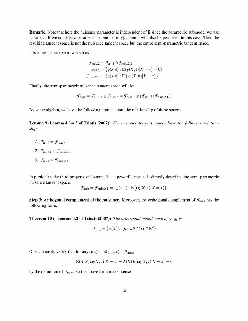
Remark. Note that here the nuisance parameter is independent of β since the parametric submodel we useis for ε|x. If we consider a parametric submodel of y|x, then β will also be perturbed in this case. Then theresulting tangent space is not the nuisance tangent space but the entire semi-parametric tangent space.

It is more instructive to write it as

Fnuis,2 = Fall,2∩Fnuis,2,1

Fall,2 = g(x,ε) : E(g(X ,ε)|X = x) = 0Fnuis,2,1 = g(x,ε) : E

(εg(X ,ε)

∣∣X = x).

Finally, the semi-parametric nuisance tangent space will be

Fnuis = Fnuis,1⊕Fnuis,2 = Fnuis,1⊕ (Fall,2∩Fnuis,2,1).

By some algebra, we have the following lemma about the relationship of these spaces.

Lemma 9 (Lemma 4.3-4.5 of Tsiatis (2007)) The nuisance tangent spaces have the following relation-ship:

1. Fall,2 = F ⊥nuis,1.

2. Fnuis,1 ⊂ Fnuis,2,1.

3. Fnuis = Fnuis,2,1.

In particular, the third property of Lemma 9 is a powerful result. It directly describes the semi-parametricnuisance tangent space:

Fnuis = Fnuis,2,1 = g(x,ε) : E(εg(X ,ε)

∣∣X = x).

Step 3: orthogonal complement of the nuisance. Moreover, the orthogonal complement of Fnuis has thefollowing form:

Theorem 10 (Theorem 4.8 of Tsiatis (2007)) The orthogonal complement of Fnuis is

F ⊥nuis = A(X)ε : for all A(x) ∈ Rq

One can easily verify that for any A(x)ε and g(x,ε) ∈ Fnuis,

E(A(X)εg(X ,ε)|X = x) = A(X)E(εg(X ,ε)|X = x) = 0

by the definition of Fnuis. So the above form makes sense.

15

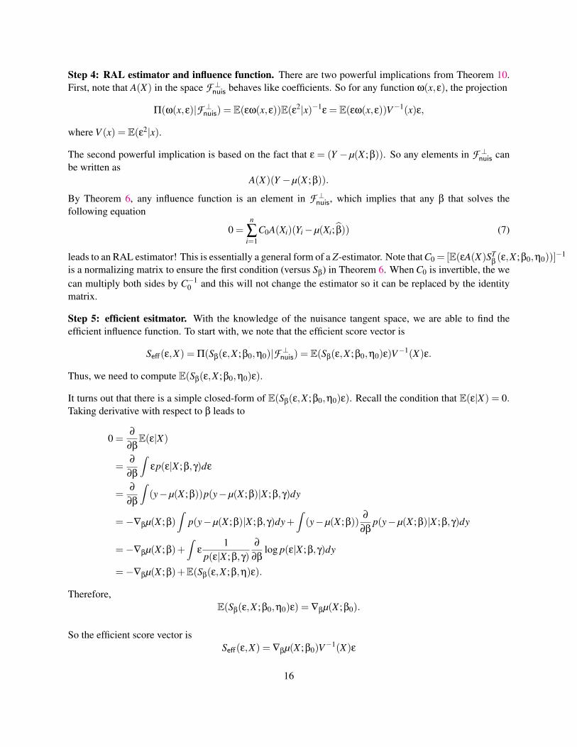
Step 4: RAL estimator and influence function. There are two powerful implications from Theorem 10.First, note that A(X) in the space F ⊥nuis behaves like coefficients. So for any function ω(x,ε), the projection

Π(ω(x,ε)|F ⊥nuis) = E(εω(x,ε))E(ε2|x)−1ε = E(εω(x,ε))V−1(x)ε,

where V (x) = E(ε2|x).

The second powerful implication is based on the fact that ε = (Y − µ(X ;β)). So any elements in F ⊥nuis canbe written as

A(X)(Y −µ(X ;β)).

By Theorem 6, any influence function is an element in F ⊥nuis, which implies that any β that solves thefollowing equation

0 =n

∑i=1

C0A(Xi)(Yi−µ(Xi; β)) (7)

leads to an RAL estimator! This is essentially a general form of a Z-estimator. Note that C0 = [E(εA(X)STβ(ε,X ;β0,η0))]

−1

is a normalizing matrix to ensure the first condition (versus Sβ) in Theorem 6. When C0 is invertible, the wecan multiply both sides by C−1

0 and this will not change the estimator so it can be replaced by the identitymatrix.

Step 5: efficient esitmator. With the knowledge of the nuisance tangent space, we are able to find theefficient influence function. To start with, we note that the efficient score vector is

Seff(ε,X) = Π(Sβ(ε,X ;β0,η0)|F ⊥nuis) = E(Sβ(ε,X ;β0,η0)ε)V−1(X)ε.

Thus, we need to compute E(Sβ(ε,X ;β0,η0)ε).

It turns out that there is a simple closed-form of E(Sβ(ε,X ;β0,η0)ε). Recall the condition that E(ε|X) = 0.Taking derivative with respect to β leads to

0 =∂

∂βE(ε|X)

=∂

∂β

∫εp(ε|X ;β,γ)dε

=∂

∂β

∫(y−µ(X ;β))p(y−µ(X ;β)|X ;β,γ)dy

=−∇βµ(X ;β)∫

p(y−µ(X ;β)|X ;β,γ)dy+∫(y−µ(X ;β))

∂

∂βp(y−µ(X ;β)|X ;β,γ)dy

=−∇βµ(X ;β)+∫

ε1

p(ε|X ;β,γ)

∂

∂βlog p(ε|X ;β,γ)dy

=−∇βµ(X ;β)+E(Sβ(ε,X ;β,η)ε).

Therefore,E(Sβ(ε,X ;β0,η0)ε) = ∇βµ(X ;β0).

So the efficient score vector isSeff(ε,X) = ∇βµ(X ;β0)V−1(X)ε

16

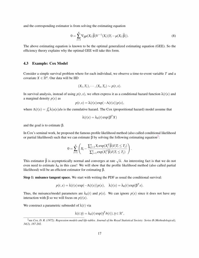
and the corresponding estimator is from solving the estimating equation

0 =n

∑i=1

∇βµ(Xi; β)V−1(Xi)(Yi−µ(Xi; β)). (8)

The above estimating equation is known to be the optimal generalized estimating equation (GEE). So theefficiency theory explains why the optimal GEE will take this form.

4.3 Example: Cox Model

Consider a simple survival problem where for each individual, we observe a time-to-event variable T and acovariate X ∈ Rq. Our data will be IID

(X1,T1), · · · ,(Xn,Tn)∼ p(t,x).

In survival analysis, instead of using p(t,x), we often express it as a conditional hazard function λ(t|x) anda marginal density p(x) as

p(t,x) = λ(t|x)exp(−Λ(t|x))p(x),

where Λ(t|x) =∫ t

0 λ(u|x)du is the cumulative hazard. The Cox (proporitional hazard) model assume that

λ(t|x) = λ0(t)exp(βT X)

and the goal is to estimate β.

In Cox’s seminal work, he proposed the famous profile likelihood method (also called conditional likelihoodor partial likelihood) such that we can estimate β by solving the following estimating equation2:

0 =n

∑i=1

(Xi−

∑nj=1 Xi exp(XT

i β)I(Ti ≤ Tj)

∑nj=1 exp(XT

i β)I(Ti ≤ Tj)

).

This estimator β is asymptotically normal and converges at rate√

n. An interesting fact is that we do noteven need to estimate λ0 in this case! We will show that the profile likelihood method (also called partiallikelihood) will be an efficient estimator for estimating β.

Step 1: nuisance tangent space. We start with writing the PDF as usual the conditional survival:

p(t,x) = λ(t|x)exp(−Λ(t|x))p(x), λ(t|x) = λ0(t)exp(βT x).

Thus, the nuisance/model parameters are λ0(t) and p(x). We can ignore p(x) since it does not have anyinteraction with β so we will focus on p(t|x).

We construct a parametric submodel of λ(t) via

λ(t;γ) = λ0(t)exp(γT b(t)),γ ∈ Rr,

2see Cox, D. R. (1972). Regression models and life-tables. Journal of the Royal Statistical Society: Series B (Methodological),34(2), 187-202.

17

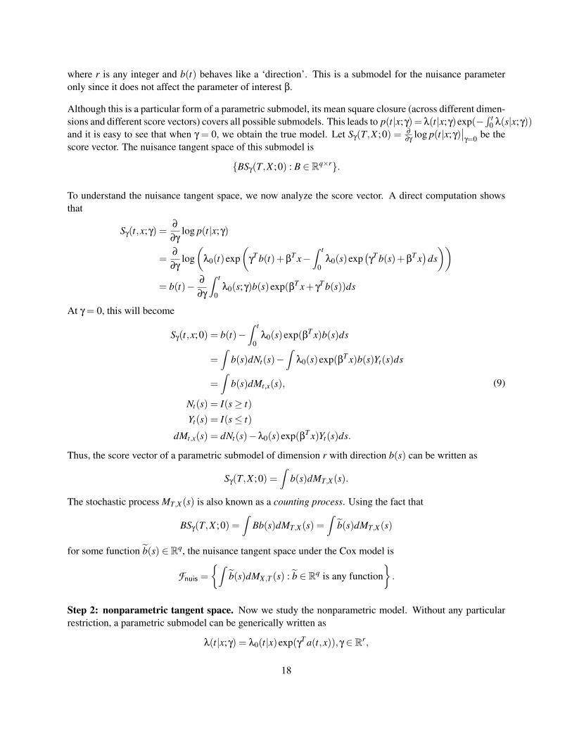
where r is any integer and b(t) behaves like a ‘direction’. This is a submodel for the nuisance parameteronly since it does not affect the parameter of interest β.

Although this is a particular form of a parametric submodel, its mean square closure (across different dimen-sions and different score vectors) covers all possible submodels. This leads to p(t|x;γ)= λ(t|x;γ)exp(−

∫ t0 λ(s|x;γ))

and it is easy to see that when γ = 0, we obtain the true model. Let Sγ(T,X ;0) = ∂

∂γlog p(t|x;γ)

∣∣γ=0 be the

score vector. The nuisance tangent space of this submodel is

BSγ(T,X ;0) : B ∈ Rq×r.

To understand the nuisance tangent space, we now analyze the score vector. A direct computation showsthat

Sγ(t,x;γ) =∂

∂γlog p(t|x;γ)

=∂

∂γlog(

λ0(t)exp(

γT b(t)+β

T x−∫ t

0λ0(s)exp

(γ

T b(s)+βT x)

ds))

= b(t)− ∂

∂γ

∫ t

0λ0(s;γ)b(s)exp(βT x+ γ

T b(s))ds

At γ = 0, this will become

Sγ(t,x;0) = b(t)−∫ t

0λ0(s)exp(βT x)b(s)ds

=∫

b(s)dNt(s)−∫

λ0(s)exp(βT x)b(s)Yt(s)ds

=∫

b(s)dMt,x(s),

Nt(s) = I(s≥ t)

Yt(s) = I(s≤ t)

dMt,x(s) = dNt(s)−λ0(s)exp(βT x)Yt(s)ds.

(9)

Thus, the score vector of a parametric submodel of dimension r with direction b(s) can be written as

Sγ(T,X ;0) =∫

b(s)dMT,X(s).

The stochastic process MT,X(s) is also known as a counting process. Using the fact that

BSγ(T,X ;0) =∫

Bb(s)dMT,X(s) =∫

b(s)dMT,X(s)

for some function b(s) ∈ Rq, the nuisance tangent space under the Cox model is

Fnuis =

∫b(s)dMX ,T (s) : b ∈ Rq is any function

.

Step 2: nonparametric tangent space. Now we study the nonparametric model. Without any particularrestriction, a parametric submodel can be generically written as

λ(t|x;γ) = λ0(t|x)exp(γT a(t,x)),γ ∈ Rr,

18

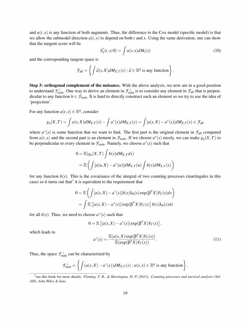
and a(t,x) is any function of both augments. Thus, the difference to the Cox model (specific model) is thatwe allow the submodel direction a(t,x) to depend on both t and x. Using the same derivation, one can showthat the tangent score will be

S†γ (t,x;0) =

∫a(s,x)dMt(s) (10)

and the corresponding tangent space is

Fall =

∫a(s,X)dMX ,T (s) : a ∈ Rq is any function

.

Step 3: orthogonal complement of the nuisance. With the above analysis, we now are in a good positionto understand F ⊥nuis. One way to derive an element in F ⊥nuis is to consider any element in Fall that is perpen-dicular to any function h ∈ Fnuis. It is hard to directly construct such an element so we try to use the idea of‘projection’.

For any function a(t,x) ∈ Rq, consider

ga(X ,T ) =∫

a(s,X)dMX ,T (s)−∫

a∗(s)dMX ,T (s) =∫[a(s,X)−a∗(s)]dMX ,T (s) ∈ Fall

where a∗(s) is some function that we want to find. The first part is the original element in Fall computedfrom a(t,x) and the second part is an element in Fnuis. If we choose a∗(s) nicely, we can make ga(X ,T ) tobe perpendicular to every element in Fnuis. Namely, we choose a∗(s) such that

0 = E(ga(X ,T )∫

b(s)dMX ,T ds)

= E(∫

[a(u,X)−a∗(u)]dMX ,T (u)∫

b(s)dMX ,T (s))

for any function b(s). This is the covariance of the integral of two counting processes (martingales in thiscase) so it turns out that3 it is equivalent to the requirement that

0 = E(∫

[a(s,X)−a∗(s)]b(s)λ0(s)exp(βT X)YT (s)ds)

=∫

E[[a(s,X)−a∗(s)]exp(βT X)YT (s)

]b(s)λ0(s)ds

for all b(s). Thus, we need to choose a∗(s) such that

0 = E[[a(s,X)−a∗(s)]exp(βT X)YT (s)

],

which leads to

a∗(s) =E(a(s,X)exp(βT X)YT (s))

E(exp(βT X)YT (s)). (11)

Thus, the space F ⊥nuis can be characterized by

F ⊥nuis =

∫(a(s,X)−a∗(s))dMX ,T (s) : a(s,x) ∈ Rq is any function

.

3see this book for more details: Fleming, T. R., & Harrington, D. P. (2011). Counting processes and survival analysis (Vol.169). John Wiley & Sons.

19

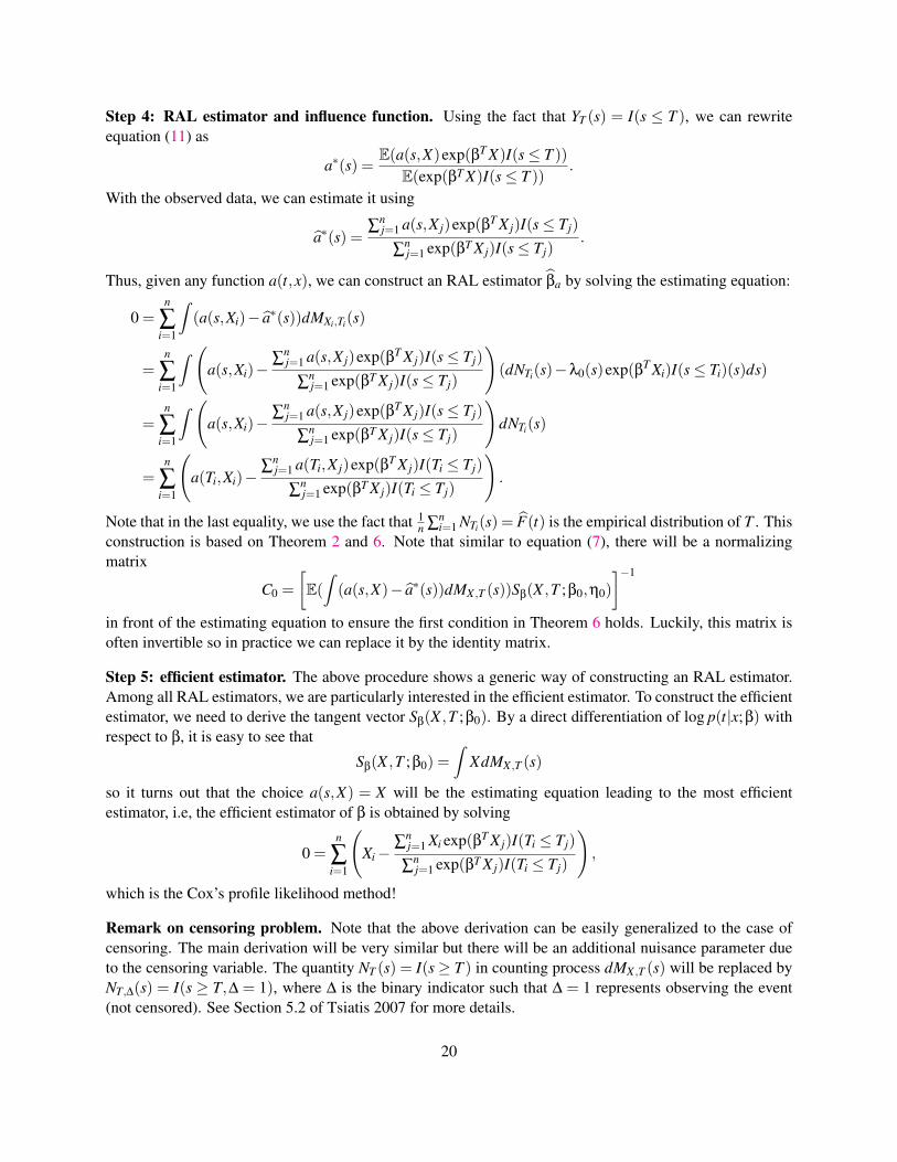
Step 4: RAL estimator and influence function. Using the fact that YT (s) = I(s ≤ T ), we can rewriteequation (11) as

a∗(s) =E(a(s,X)exp(βT X)I(s≤ T ))

E(exp(βT X)I(s≤ T )).

With the observed data, we can estimate it using

a∗(s) =∑

nj=1 a(s,X j)exp(βT X j)I(s≤ Tj)

∑nj=1 exp(βT X j)I(s≤ Tj)

.

Thus, given any function a(t,x), we can construct an RAL estimator βa by solving the estimating equation:

0 =n

∑i=1

∫(a(s,Xi)− a∗(s))dMXi,Ti(s)

=n

∑i=1

∫ (a(s,Xi)−

∑nj=1 a(s,X j)exp(βT X j)I(s≤ Tj)

∑nj=1 exp(βT X j)I(s≤ Tj)

)(dNTi(s)−λ0(s)exp(βT Xi)I(s≤ Ti)(s)ds)

=n

∑i=1

∫ (a(s,Xi)−

∑nj=1 a(s,X j)exp(βT X j)I(s≤ Tj)

∑nj=1 exp(βT X j)I(s≤ Tj)

)dNTi(s)

=n

∑i=1

(a(Ti,Xi)−

∑nj=1 a(Ti,X j)exp(βT X j)I(Ti ≤ Tj)

∑nj=1 exp(βT X j)I(Ti ≤ Tj)

).

Note that in the last equality, we use the fact that 1n ∑

ni=1 NTi(s) = F(t) is the empirical distribution of T . This

construction is based on Theorem 2 and 6. Note that similar to equation (7), there will be a normalizingmatrix

C0 =

[E(

∫(a(s,X)− a∗(s))dMX ,T (s))Sβ(X ,T ;β0,η0)

]−1

in front of the estimating equation to ensure the first condition in Theorem 6 holds. Luckily, this matrix isoften invertible so in practice we can replace it by the identity matrix.

Step 5: efficient estimator. The above procedure shows a generic way of constructing an RAL estimator.Among all RAL estimators, we are particularly interested in the efficient estimator. To construct the efficientestimator, we need to derive the tangent vector Sβ(X ,T ;β0). By a direct differentiation of log p(t|x;β) withrespect to β, it is easy to see that

Sβ(X ,T ;β0) =∫

XdMX ,T (s)

so it turns out that the choice a(s,X) = X will be the estimating equation leading to the most efficientestimator, i.e, the efficient estimator of β is obtained by solving

0 =n

∑i=1

(Xi−

∑nj=1 Xi exp(βT X j)I(Ti ≤ Tj)

∑nj=1 exp(βT X j)I(Ti ≤ Tj)

),

which is the Cox’s profile likelihood method!

Remark on censoring problem. Note that the above derivation can be easily generalized to the case ofcensoring. The main derivation will be very similar but there will be an additional nuisance parameter dueto the censoring variable. The quantity NT (s) = I(s≥ T ) in counting process dMX ,T (s) will be replaced byNT,∆(s) = I(s ≥ T,∆ = 1), where ∆ is the binary indicator such that ∆ = 1 represents observing the event(not censored). See Section 5.2 of Tsiatis 2007 for more details.

20

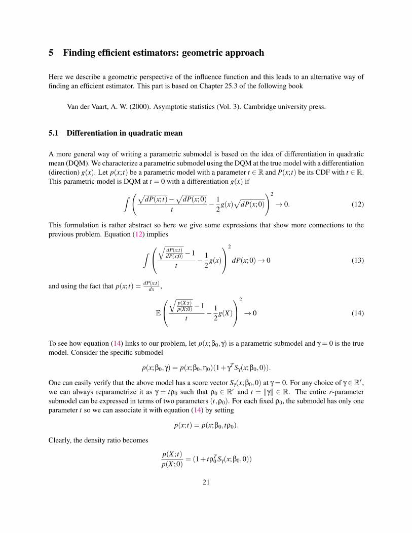
5 Finding efficient estimators: geometric approach

Here we describe a geometric perspective of the influence function and this leads to an alternative way offinding an efficient estimator. This part is based on Chapter 25.3 of the following book

Van der Vaart, A. W. (2000). Asymptotic statistics (Vol. 3). Cambridge university press.

5.1 Differentiation in quadratic mean

A more general way of writing a parametric submodel is based on the idea of differentiation in quadraticmean (DQM). We characterize a parametric submodel using the DQM at the true model with a differentiation(direction) g(x). Let p(x; t) be a parametric model with a parameter t ∈R and P(x; t) be its CDF with t ∈R.This parametric model is DQM at t = 0 with a differentiation g(x) if

∫ (√dP(x; t)−√

dP(x;0)t

− 12

g(x)√

dP(x;0)

)2

→ 0. (12)

This formulation is rather abstract so here we give some expressions that show more connections to theprevious problem. Equation (12) implies

∫ √

dP(x;t)dP(x;0) −1

t− 1

2g(x)

2

dP(x;0)→ 0 (13)

and using the fact that p(x; t) = dP(x;t)dx ,

E

√

p(X ;t)p(X ;0) −1

t− 1

2g(X)

2

→ 0 (14)

To see how equation (14) links to our problem, let p(x;β0,γ) is a parametric submodel and γ = 0 is the truemodel. Consider the specific submodel

p(x;β0,γ) = p(x;β0,η0)(1+ γT Sγ(x;β0,0)).

One can easily verify that the above model has a score vector Sγ(x;β0,0) at γ = 0. For any choice of γ ∈Rr,we can always reparametrize it as γ = tρ0 such that ρ0 ∈ Rr and t = ‖γ‖ ∈ R. The entire r-parametersubmodel can be expressed in terms of two parameters (t,ρ0). For each fixed ρ0, the submodel has only oneparameter t so we can associate it with equation (14) by setting

p(x; t) = p(x;β0, tρ0).

Clearly, the density ratio becomes

p(X ; t)p(X ;0)

= (1+ tρT0 Sγ(x;β0,0))

21

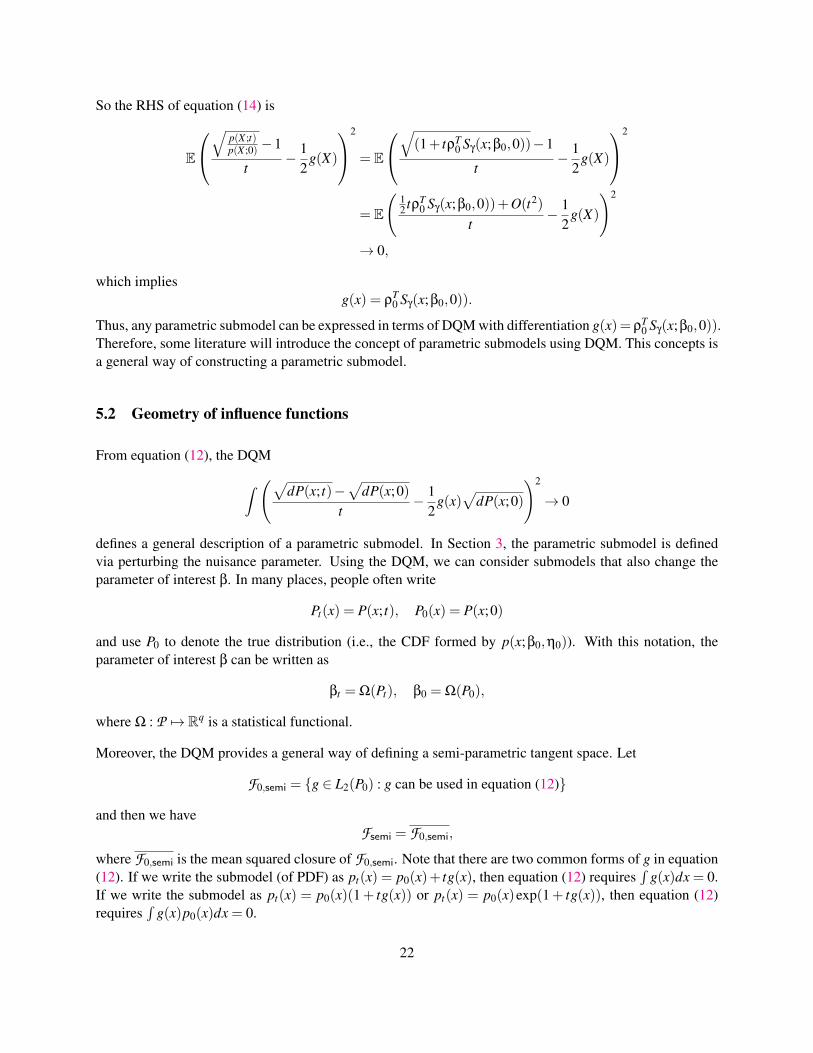
So the RHS of equation (14) is

E

√

p(X ;t)p(X ;0) −1

t− 1

2g(X)

2

= E

√(1+ tρT

0 Sγ(x;β0,0))−1

t− 1

2g(X)

2

= E

(12 tρT

0 Sγ(x;β0,0))+O(t2)

t− 1

2g(X)

)2

→ 0,

which impliesg(x) = ρ

T0 Sγ(x;β0,0)).

Thus, any parametric submodel can be expressed in terms of DQM with differentiation g(x)= ρT0 Sγ(x;β0,0)).

Therefore, some literature will introduce the concept of parametric submodels using DQM. This concepts isa general way of constructing a parametric submodel.

5.2 Geometry of influence functions

From equation (12), the DQM

∫ (√dP(x; t)−√

dP(x;0)t

− 12

g(x)√

dP(x;0)

)2

→ 0

defines a general description of a parametric submodel. In Section 3, the parametric submodel is definedvia perturbing the nuisance parameter. Using the DQM, we can consider submodels that also change theparameter of interest β. In many places, people often write

Pt(x) = P(x; t), P0(x) = P(x;0)

and use P0 to denote the true distribution (i.e., the CDF formed by p(x;β0,η0)). With this notation, theparameter of interest β can be written as

βt = Ω(Pt), β0 = Ω(P0),

where Ω : P 7→ Rq is a statistical functional.

Moreover, the DQM provides a general way of defining a semi-parametric tangent space. Let

F0,semi = g ∈ L2(P0) : g can be used in equation (12)

and then we haveFsemi = F0,semi,

where F0,semi is the mean squared closure of F0,semi. Note that there are two common forms of g in equation(12). If we write the submodel (of PDF) as pt(x) = p0(x)+ tg(x), then equation (12) requires

∫g(x)dx = 0.

If we write the submodel as pt(x) = p0(x)(1+ tg(x)) or pt(x) = p0(x)exp(1+ tg(x)), then equation (12)requires

∫g(x)p0(x)dx = 0.

22

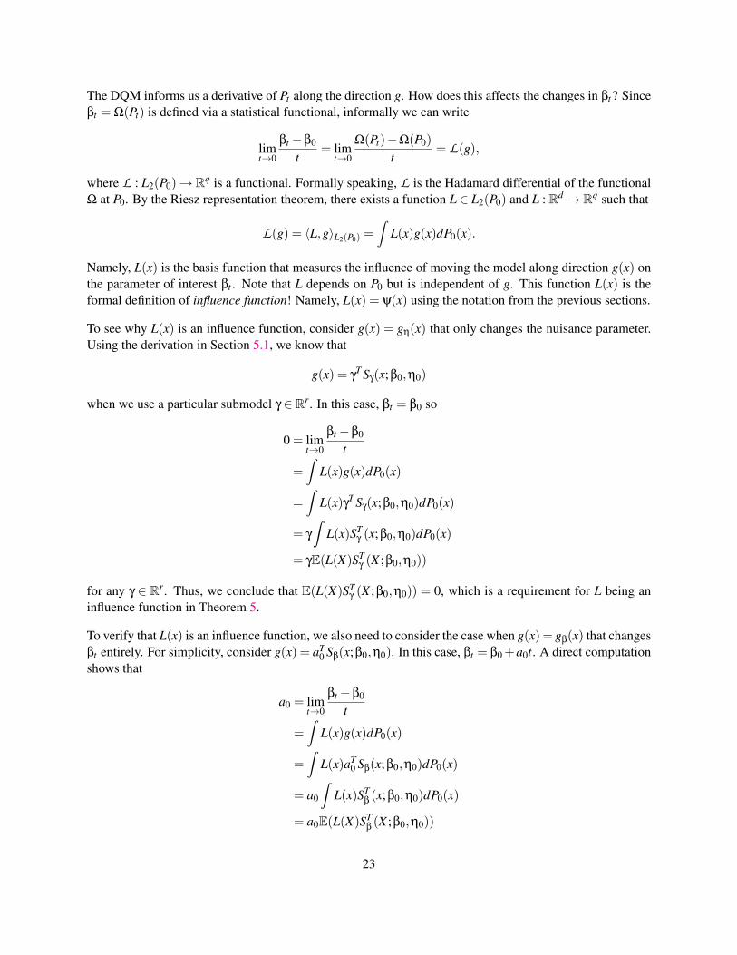
The DQM informs us a derivative of Pt along the direction g. How does this affects the changes in βt? Sinceβt = Ω(Pt) is defined via a statistical functional, informally we can write

limt→0

βt −β0

t= lim

t→0

Ω(Pt)−Ω(P0)

t= L(g),

where L : L2(P0)→ Rq is a functional. Formally speaking, L is the Hadamard differential of the functionalΩ at P0. By the Riesz representation theorem, there exists a function L ∈ L2(P0) and L : Rd → Rq such that

L(g) = 〈L,g〉L2(P0) =∫

L(x)g(x)dP0(x).

Namely, L(x) is the basis function that measures the influence of moving the model along direction g(x) onthe parameter of interest βt . Note that L depends on P0 but is independent of g. This function L(x) is theformal definition of influence function! Namely, L(x) = ψ(x) using the notation from the previous sections.

To see why L(x) is an influence function, consider g(x) = gη(x) that only changes the nuisance parameter.Using the derivation in Section 5.1, we know that

g(x) = γT Sγ(x;β0,η0)

when we use a particular submodel γ ∈ Rr. In this case, βt = β0 so

0 = limt→0

βt −β0

t

=∫

L(x)g(x)dP0(x)

=∫

L(x)γT Sγ(x;β0,η0)dP0(x)

= γ

∫L(x)ST

γ (x;β0,η0)dP0(x)

= γE(L(X)STγ (X ;β0,η0))

for any γ ∈ Rr. Thus, we conclude that E(L(X)STγ (X ;β0,η0)) = 0, which is a requirement for L being an

influence function in Theorem 5.

To verify that L(x) is an influence function, we also need to consider the case when g(x) = gβ(x) that changesβt entirely. For simplicity, consider g(x) = aT

0 Sβ(x;β0,η0). In this case, βt = β0+a0t. A direct computationshows that

a0 = limt→0

βt −β0

t

=∫

L(x)g(x)dP0(x)

=∫

L(x)aT0 Sβ(x;β0,η0)dP0(x)

= a0

∫L(x)ST

β(x;β0,η0)dP0(x)

= a0E(L(X)STβ(X ;β0,η0))

23

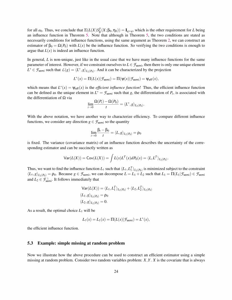
for all a0. Thus, we conclude that E(L(X)STβ(X ;β0,η0)) = Iq×q, which is the other requirement for L being

an influence function in Theorem 5. Note that although in Theorem 5, the two conditions are stated asnecessarily conditions for influence functions, using the same argument as Theorem 2, we can construct anestimator of β0 = Ω(P0) with L(x) be the influence function. So verifying the two conditions is enough toargue that L(x) is indeed an influence function.

In general, L is non-unique, just like in the usual case that we have many influence functions for the sameparameter of interest. However, if we constraint ourselves to L∈Fsemi, then there is only one unique elementL∗ ∈ Fsemi such that L(g) = 〈L∗,g〉L2(P0). And it can be characterized by the projection

L∗(x) = Π(L(x)|Fsemi) = Π(ψ(x)|Fsemi) = ψeff(x),

which means that L∗(x) = ψeff(x) is the efficient influence function! Thus, the efficient influence functioncan be defined as the unique element in L∗ = Fsemi such that g, the differentiation of Pt , is associated withthe differentiation of Ω via

limt→0

Ω(Pt)−Ω(P0)

t= 〈L∗,g〉L2(P0).

With the above notation, we have another way to characterize efficiency. To compare different influencefunctions, we consider any direction g ∈ Fsemi so the quantity

limt→0

βt −β0

t= 〈L,g〉L2(P0) = ρ0

is fixed. The variance (covariance matrix) of an influence function describes the uncertainty of the corre-sponding estimator and can be succinctly written as

Var(L(X)) = Cov(L(X)) =∫

L(x)LT (x)dP0(x) = 〈L,LT 〉L2(P0).

Thus, we want to find the influence function L† such that 〈L†,LT† 〉L2(P0) is minimized subject to the constraint

〈L†,g〉L2(P0) = ρ0. Because g ∈ Fsemi, we can decompose L = L1 +L2 such that L1 = Π(L1|Fsemi) ∈ Fsemi

and L2 ∈ F ⊥semi. It follows immediately that

Var(L(X)) = 〈L1,LT1 〉L2(P0)+ 〈L2,LT

2 〉L2(P0)

〈L1,g〉L2(P0) = ρ0

〈L2,g〉L2(P0) = 0.

As a result, the optimal choice L† will be

L†(x) = L1(x) = Π(L(x)|Fsemi) = L∗(x),

the efficient influence function.

5.3 Example: simple missing at random problem

Now we illustrate how the above procedure can be used to construct an efficient estimator using a simplemissing at random problem. Consider two random variables problem: X ,Y . X is the covariate that is always

24

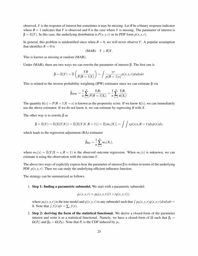
observed. Y is the response of interest but sometimes it may be missing. Let R be a binary response indicatorwhere R = 1 indicates that Y is observed and 0 is the case where Y is missing. The parameter of interest isβ = E(Y ). In this case, the underlying distribution is P(x,y,r) or its PDF form p(x,y,r).

In general, this problem is unidentified since when R = 0, we will never observe Y . A popular assumptionthat identifies R = 0 is

(MAR) Y ⊥ R|X .

This is known as missing at random (MAR).

Under (MAR), there are two ways we can rewrite the parameter of interest β. The first one is

β = E(Y ) = E(

Y RP(R = 1|X)

)=

∫ yrp(R = 1|x)

p(x,y,r)dxdydr.

This is related to the inverse probability weighting (IPW) estimator since we can estimate β via

βIPW =1n

n

∑i=1

YiRi

P(R = 1|Xi)=

1n

n

∑i=1

YiRi

π(Xi).

The quantity π(x) = P(R = 1|X = x) is known as the propensity score. If we know π(x), we can immediatelyuse the above estimator. If we do not know it, we can estimate by regressing R with X .

The other way is to rewrite β as

β = E(Y ) = E(E(Y |X)) = E(E(Y |X ,R = 1)) = E(m1(X)) =∫ ∫

yp(y|x,R = 1)dyp(x)dx,

which leads to the regression adjustment (RA) estimator

βRA =1n

n

∑i=1

m1(Xi),

where m1(x) = E(Y |X = x,R = 1) is the observed outcome regression. When m1(x) is unknown, we canestimate it using the observation with the outcome Y .

The above two ways of explicitly express how the parameter of interest β is written in terms of the underlyingPDF p(x,y,r). Then we can study the underlying efficient influence function.

The strategy can be summarized as follows.

1. Step 1: finding a parametric submodel. We start with a parametric submodel:

pt(x,y,r) = p0(x,y,r)(1+ tg(x,y,r)),

where p0(x,y,r) is the true model and g(x,y,r) is any submodel such that∫

p0(x,y,r)g(x,y,r)dxdydr =0. Note that

∫f (r)dr = ∑r f (r).

2. Step 2: deriving the form of the statistical functional. We derive a closed-form of the parameterinterest and write it as a statistical functional. Namely, we have a closed-form of Ω such that βt =Ω(Pt) and β0 = Ω(P0). Note that Pt is the CDF induced by pt .

25

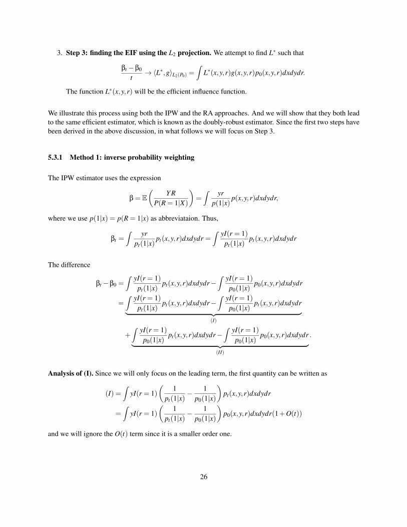
3. Step 3: finding the EIF using the L2 projection. We attempt to find L∗ such that

βt −β0

t→ 〈L∗,g〉L2(P0) =

∫L∗(x,y,r)g(x,y,r)p0(x,y,r)dxdydr.

The function L∗(x,y,r) will be the efficient influence function.

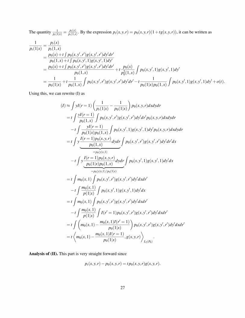
We illustrate this process using both the IPW and the RA approaches. And we will show that they both leadto the same efficient estimator, which is known as the doubly-robust estimator. Since the first two steps havebeen derived in the above discussion, in what follows we will focus on Step 3.

5.3.1 Method 1: inverse probability weighting

The IPW estimator uses the expression

β = E(

Y RP(R = 1|X)

)=

∫ yrp(1|x)

p(x,y,r)dxdydr,

where we use p(1|x) = p(R = 1|x) as abbreviataion. Thus,

βt =∫ yr

pt(1|x)pt(x,y,r)dxdydr =

∫ yI(r = 1)pt(1|x)

pt(x,y,r)dxdydr

The difference

βt −β0 =∫ yI(r = 1)

pt(1|x)pt(x,y,r)dxdydr−

∫ yI(r = 1)p0(1|x)

p0(x,y,r)dxdydr

=∫ yI(r = 1)

pt(1|x)pt(x,y,r)dxdydr−

∫ yI(r = 1)p0(1|x)

pt(x,y,r)dxdydr︸ ︷︷ ︸(I)

+∫ yI(r = 1)

p0(1|x)pt(x,y,r)dxdydr−

∫ yI(r = 1)p0(1|x)

p0(x,y,r)dxdydr︸ ︷︷ ︸(II)

.

Analysis of (I). Since we will only focus on the leading term, the first quantity can be written as

(I) =∫

yI(r = 1)(

1pt(1|x)

− 1p0(1|x)

)pt(x,y,r)dxdydr

=∫

yI(r = 1)(

1pt(1|x)

− 1p0(1|x)

)p0(x,y,r)dxdydr(1+O(t))

and we will ignore the O(t) term since it is a smaller order one.

26

The quantity 1pt(1|x) =

pt(x)pt(1,x)

. By the expression pt(x,y,r) = p0(x,y,r)(1+ tg(x,y,r)), it can be written as

1pt(1|x)

=pt(x)

pt(1,x)

=p0(x)+ t

∫p0(x,y′,r′)g(x,y′,r′)dy′dr′

p0(1,x)+ t∫

p0(x,y′,1)g(x,y′,1)dy′

=p0(x)+ t

∫p0(x,y′,r′)g(x,y′,r′)dy′dr′

p0(1,x)+ t

p0(x)p2

0(1,x)

∫p0(x,y′,1)g(x,y′,1)dy′

=1

p0(1|x)+ t

1p0(1,x)

∫p0(x,y′,r′)g(x,y′,r′)dy′dr′− t

1p0(1|x)p0(1,x)

∫p0(x,y′,1)g(x,y′,1)dy′+o(t).

Using this, we can rewrite (I) as

(I)≈∫

yI(r = 1)(

1pt(1|x)

− 1p0(1|x)

)p0(x,y,r)dxdydr

= t∫ yI(r = 1)

p0(1,x)

∫p0(x,y′,r′)g(x,y′,r′)dy′dr′p0(x,y,r)dxdydr

− t∫ yI(r = 1)

p0(1|x)p0(1,x)

∫p0(x,y′,1)g(x,y′,1)dy′p0(x,y,r)dxdydr

= t∫

yI(r = 1)p0(x,y,r)

p0(1,x)dydr︸ ︷︷ ︸

=p0(y|x,1)

∫p0(x,y′,r′)g(x,y′,r′)dy′dr′dx

− t∫

yI(r = 1)p0(x,y,r)

p0(1|x)p0(1,x)dydr︸ ︷︷ ︸

=p0(y|x,1)/p0(1|x)

∫p0(x,y′,1)g(x,y′,1)dy′dx

= t∫

m0(x,1)∫

p0(x,y′,r′)g(x,y′,r′)dy′dxdr′

− t∫ m0(x,1)

p(1|x)

∫p0(x,y′,1)g(x,y′,1)dy′dx

= t∫

m0(x,1)∫

p0(x,y′,r′)g(x,y′,r′)dy′dxdr′

− t∫ m0(x,1)

p(1|x)

∫I(r′ = 1)p0(x,y′,r′)g(x,y′,r′)dy′dxdr′

= t∫ (

m0(x,1)−m0(x,1)I(r′ = 1)

p0(1|x)

)p0(x,y′,r′)g(x,y′,r′)dy′dxdr′

= t⟨

m0(x,1)−m0(x,1)I(r = 1)

p0(1|x),g(x,y,r)

⟩L2(P0)

.

Analysis of (II). This part is very straight forward since

pt(x,y,r)− p0(x,y,r) = t p0(x,y,r)g(x,y,r).

27

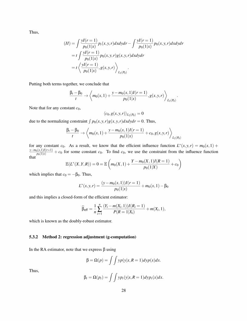
Thus,

(II) =∫ yI(r = 1)

p0(1|x)pt(x,y,r)dxdydr−

∫ yI(r = 1)p0(1|x)

p0(x,y,r)dxdydr

= t∫ yI(r = 1)

p0(1|x)p0(x,y,r)g(x,y,r)dxdydr

= t⟨

yI(r = 1)p0(1|x)

,g(x,y,r)⟩

L2(P0)

.

Putting both terms together, we conclude that

βt −β0

t→⟨

m0(x,1)+y−m0(x,1)I(r = 1)

p0(1|x),g(x,y,r)

⟩L2(P0)

.

Note that for any constant c0,〈c0,g(x,y,r)〉L2(P0) = 0

due to the normalizing constraint∫

p0(x,y,r)g(x,y,r)dxdydr = 0. Thus,

βt −β0

t→⟨

m0(x,1)+y−m0(x,1)I(r = 1)

p0(1|x)+ c0,g(x,y,r)

⟩L2(P0)

for any constant c0. As a result, we know that the efficient influence function L∗(x,y,r) = m0(x,1) +y−m0(x,1)I(r=1)

p0(1|x) + c0 for some constant c0. To find c0, we use the constraint from the influence functionthat

E(L∗(X ,Y,R)) = 0 = E(

m0(X ,1)+Y −m0(X ,1)I(R = 1)

p0(1|X)+ c0

)which implies that c0 =−β0. Thus,

L∗(x,y,r) =(y−m0(x,1))I(r = 1)

p0(1|x)+m0(x,1)−β0

and this implies a closed-form of the efficient estimator:

βeff =1n

n

∑i=1

(Yi−m(Xi,1))I(Ri = 1)P(R = 1|Xi)

+m(Xi,1),

which is known as the doubly-robust estimator.

5.3.2 Method 2: regression adjustment (g-computation)

In the RA estimator, note that we express β using

β = Ω(p) =∫ ∫

yp(y|x,R = 1)dyp(x)dx.

Thus,βt = Ω(pt) =

∫ ∫ypt(y|x,R = 1)dypt(x)dx.

28

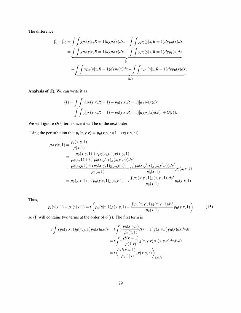
The difference

βt −β0 =∫ ∫

ypt(y|x,R = 1)dypt(x)dx.−∫ ∫

yp0(y|x,R = 1)dyp0(x)dx

=∫ ∫

ypt(y|x,R = 1)dypt(x)dx.−∫ ∫

yp0(y|x,R = 1)dypt(x)dx︸ ︷︷ ︸(I)

+∫ ∫

yp0(y|x,R = 1)dypt(x)dx−∫ ∫

yp0(y|x,R = 1)dyp0(x)dx︸ ︷︷ ︸(II)

.

Analysis of (I). We can write it as

(I) =∫ ∫

y[pt(y|x,R = 1)− p0(y|x,R = 1)]dypt(x)dx

=∫ ∫

y[pt(y|x,R = 1)− p0(y|x,R = 1)]dyp0(x)dx(1+O(t)).

We will ignore O(t) term since it will be of the next order.

Using the perturbation that pt(x,y,r) = p0(x,y,r)(1+ tg(x,y,r)),

pt(y|x,1) =pt(x,y,1)

p(x,1)

=p0(x,y,1)+ t p0(x,y,1)g(x,y,1)

p0(x,1)+ t∫

p0(x,y′,r)g(x,y′,r))dy′

=p0(x,y,1)+ t p0(x,y,1)g(x,y,1)

p0(x,1)− t

∫p0(x,y′,r)g(x,y′,r))dy′

p20(x,1)

p0(x,y,1)

= p0(y|x,1)+ t p0(y|x,1)g(x,y,1)− t∫

p0(x,y′,1)g(x,y′,1))dy′

p0(x,1)p0(y|x,1)

Thus,

pt(y|x,1)− p0(y|x,1) = t(

p0(y|x,1)g(x,y,1)−∫

p0(x,y′,1)g(x,y′,1)dy′

p0(x,1)p0(y|x,1)

)(15)

so (I) will contains two terms at the order of O(t). The first term is

t∫

yp0(y|x,1)g(x,y,1)p0(x)dxdy = t∫

yp0(x,y,r)p0(x,1)

I(r = 1)g(x,y,r)p0(x)dxdydr

= t∫

yyI(r = 1)

p(1|x)g(x,y,r)p0(x,y,r)dxdydr

= t⟨

yI(r = 1)p0(1|x)

,g(x,y,r)⟩

L2(P0)

.

29

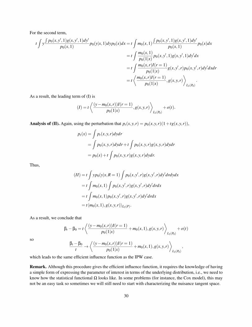
For the second term,

t∫

y∫

p0(x,y′,1)g(x,y′,1)dy′

p0(x,1)p0(y|x,1)dyp0(x)dx = t

∫m0(x,1)

∫p0(x,y′,1)g(x,y′,1)dy′

p0(x,1)p0(x)dx

= t∫ m0(x,1)

p0(1|x)p0(x,y′,1)g(x,y′,1)dy′dx

= t∫ m0(x,r)I(r = 1)

p0(1|x)g(x,y′,r)p0(x,y′,r)dy′dxdr

= t⟨

m0(x,r)I(r = 1)p0(1|x)

,g(x,y,r)⟩

L2(P0)

.

As a result, the leading term of (I) is

(I) = t⟨(y−m0(x,r))I(r = 1)

p0(1|x),g(x,y,r)

⟩L2(P0)

+o(t).

Analysis of (II). Again, using the perturbation that pt(x,y,r) = p0(x,y,r)(1+ tg(x,y,r)),

pt(x) =∫

pt(x,y,r)dydr

=∫

p0(x,y,r)dydr+ t∫

p0(x,y,r)g(x,y,r)dydr

= p0(x)+ t∫

p0(x,y,r)g(x,y,r)dydr.

Thus,

(II) = t∫

yp0(y|x,R = 1)∫

p0(x,y′,r)g(x,y′,r)dy′drdydx

= t∫

m0(x,1)∫

p0(x,y′,r)g(x,y′,r)dy′drdx

= t∫

m0(x,1)p0(x,y′,r)g(x,y′,r)dy′drdx

= t〈m0(x,1),g(x,y,r)〉L2(P).

As a result, we conclude that

βt −β0 = t⟨(y−m0(x,r))I(r = 1)

p0(1|x)+m0(x,1),g(x,y,r)

⟩L2(P0)

+o(t)

soβt −β0

t→⟨(y−m0(x,r))I(r = 1)

p0(1|x)+m0(x,1),g(x,y,r)

⟩L2(P0)

,

which leads to the same efficient influence function as the IPW case.

Remark. Although this procedure gives the efficient influence function, it requires the knowledge of havinga simple form of expressing the parameter of interest in terms of the underlying distribution, i.e., we need toknow how the statistical functional Ω looks like. In some problems (for instance, the Cox model), this maynot be an easy task so sometimes we will still need to start with characterizing the nuisance tangent space.

30

5.4 More about DQM

The concept of DQM appears in many analysis of a parametric model. In particular, when we are dealingwith the problem of local alternatives–a sequence of model that is very close to the true model but wecan still derive meaningful results. This gives us some hints on why we may use it as a way to constructparametric submodels. The key part of a parametric submodel is its behavior close to the true model.

To see how DQM is useful in local alternatives, consider IID observations X1, · · · ,Xn from an unknownparametric density p(x;θ0). The collection p(x;θ) : θ ∈ Θ is the parametric model we are considering.Consider a sequence hn→ 0 and a sequence of models p(x;θ0 +hn) and the hypothesis testing problem:

H0 : θ = θ0, Ha,n : θ = θ0 +hn.

Note that the alternative hypothesis changes when n→ 0.

When hn converges too fast, we will not be able to distinguish the two hypothesis. When hn converges tooslow, the problem is trivial in the sense that we can easily distinguish the two hypothesis. However, there isan interesting regime where when hn converges to 0 at a particular rate, we will see interesting results.

Specifically, consider the likelihood ratio test (since it is the uniformly most powerful test in the simpleversus simple tests) and the test statistic

λn =n

∑i=1

logp(Xi;θ0 +hn)

p(Xi;θ0).

To obtain a regular asymptotic results in a likelihood model, we often assume that the likelihood function istwice-differentiable to obtain a reasonable Fisher’s information matrix.

But here is an interesting fact: we do not need twice-differentiation in this local alternative case. What weneed is that p(x;θ) is DQM in a neighborhood of θ0.

To see this, note that the DQM in a multivariate case can be written as (using the form of equation (14))

∫ (√p(x;θ0 +hn)−

√p(x;θ0)−

12

hTn `′(θ0|x)

√p(x;θ0)

)2

dx = o(‖hn‖2),

where `′(θ|x) = ∂

∂θ`(θ|x) = ∂

∂θp(x;θ) is the score of the likelihood model. Let

δn(x) =√

p(x;θ0 +hn)−√

p(x;θ0)−12

hTn `′(θ0|x)

√p(x;θ0).

The DQM requires ‖δn‖2L2(P)

= o(‖hn‖2).

31

Using the DQM, we can rewrite the test statistic as

λn =n

∑i=1

logp(Xi;θ0 +hn)

p(Xi;θ0)

= 2n

∑i=1

log

√p(Xi;θ0 +hn)

p(Xi;θ0)

= 2n

∑i=1

log

√p(Xi;θ0)+

12 hT

n `′(θ0|Xi)

√p(Xi;θ0)+δn(Xi)√

p(Xi;θ0)

= 2n

∑i=1

log(

1+12

hTn `′(θ0|Xi)+oP(‖hn‖)

)≈ 2

n

∑i=1

(12

hTn `′(θ0|Xi)−

14

hTn `′(θ0|Xi)`

′T (θ0|Xi)hn

)=√

nhn1√n

n

∑i=1

`′(θ0|Xi)−12√

nhTn

[1n

n

∑i=1

`′(θ0|Xi)`′T (θ0|Xi)

]√

nhn.

Therefore, if we choose hn = n−1/2c0 for some constant c0, we obtain

λn = c01√n

Zn−12

cT0 In(θ0)c0,

where Znd→ N(0, I(θ0)) and

I(θ0) = E(`′(θ0|X1)`′T (θ0|X1))

is the information matrix and

In(θ0) =1n

n

∑i=1

`′(θ0|Xi)`′T (θ0|Xi)

p→ I(θ0).

By the Slutsky’s theorem,

λnd→ N

(−1

2cT

0 I(θ0)c0,cT0 I(θ0)c0

),

a regular distribution!

This gives us two conclusions:

• Convergence rate of local alternatives. The rate hn = n−1/2c0 is the critical rate such that if a localalternative converges faster than this, then there is no way to distinguish them (H0 and Ha) and if thelocal alternative converges slower than this, then we have an asymptotic probability 1 to distinguishthem.

• Differentiation in quadratic mean. In our analysis, we did not assume that the likelihood functionis twice differentiable. All we need is the DQM. Thus, DQM can be viewed as a weak condition thatallows us to work on the neighborhood of the true model. This explains why many literature use DQMas a way to specify a parametric submodel.

32

6 Finding efficient estimators: conditional expectation

Let X be a random variable and let Z = m(X) for some known fixed function m. Let P be the distributionof X and Q be the distribution of Z. The tangent space of X and the tangent space of Z are associated asfollows.

Theorem 11 (Lemma 25.34 of van der Vaart 2000) Assume the above notations. Suppose that P is DQMwith respect to direction g(x). Then Q is DQM with respect to direction w(z)

w(z) = E(g(X)|Z = z).

If we view w(z) = Ag(z), where A : L2(P)→ L2(Q) is an operator, then its adjoint A∗ : L2(Q)→ L2(P) canbe expressed as

A∗h(x) = E(h(Z)|X = x).

The power of Theorem 11 is that it converts any parametric submodel of X into a parametric submodel ofZ = m(X). This is useful because Z is often something that we observe (so it contains less information thanX) but we want to consider a submodel over the full variable X .

Example: censoring. Consider a simple censoring problem where we observe (Y,∆) such that Y =minT,Cand ∆ = I(Y = T ) and T is the outcome of interest and C is the censoring time. We assume that both T,C≥ 0and T ⊥C. Let p(y,δ) be the PDF of the observed variables and pT (t) and pC(t) be the PDF of T and C.We use the subscript to denote the true model, i.e., p0(y,δ) is the PDF that generates our data and pT,0, pC,0are the true PDF of T and C.

Because T and C are independent, any parametric submodel of pT,C that preserves the independence can bedecomposed into the a submodel of pT and a submodel of pC. Theorem 11 shows that if we can convert anyparametric submodel of pT (t) into a parametric submodel of p(y,δ). Consider a parametric submodel

pT,ε(t) = pT,0(t)(1+ εg(t)).

Then by Theorem 11, this submodel will imply the follow parametric submodel of pε(y,δ):

pε(y,δ) = p0(y,δ)(1+ εw(y,δ)),

where

w(y,δ) = E(g(T )|Y = y,∆ = δ) = δg(y)+(1−δ)

∫∞

y g(t)pT,0(t)dt

1−FT,0(y). (16)

For the censoring variable, a similar analysis shows that if pC(c) is DQM with direction q(c), then the p(y,δ)is DQM with direction ξ(y,δ)

ξ(y,δ) = E(q(C)|Y = y,∆ = δ)

= (1−δ)q(y)+δ

∫∞

y q(c)pC,0(c)dc

1−FC,0(y).

33

6.1 Finding a computable influence function and efficient estimator

In general, the parameter of interest β will be a statistical functional of the complete data X . We oftenhave an RAL estimator with an influence function ψ(x) for β. Theorem 11 immediately implies that for theobserved data (Z), the corresponding influence function will be

ψ∗(z) = E(ψ(X)|Z = z).

This is because by definition, an influence function has mean 0 so it can always be used as a submodeldirection. Thus, this immediately gives us an estimator using the observed data. Alternatively, using thesecond statement of Theorem 11, another strategy of finding an influence function using the observed datais to find ψ†(z) such that

E(ψ†(Z)|X = x) = ψ(x).

Sometimes, the first strategy is useful and sometimes the second one is better. To illustrate the idea, considerthe following current status model.

6.2 Example: current status model

In the current status model, there are two positive random variables T and Y . T is the outcome variable ofinterest but is unobserved. Y is a measurement time point that is always observed. The observed data is

(Y1,∆1), · · · ,(Yn,∆n),

where ∆ = I(T ≤ Y ) is a status variable denoting if the event occurs before the measurement time (i.e.,T ≤ Y ). We assume that T and Y are independent.

Let pT , pY be the PDF of T and Y and PT ,PY be the corresponding CDFs. The observed-data density (PDFcorresponding to the observed data) is

p(y,δ) = pY (y)PT (y)δ(1−PT (y))1−δ,

The conditional densities

p(y,δ|T = t) = δpY (y)I(y≥ t)

1−PY (t)+(1−δ)

pY (y)I(y < t)PY (t)

,

p(t|Y = y,∆ = δ) = δpT (t)PT (y)

I(t ≤ y)+(1−δ)pT (t)

1−PT (y)I(t > y).

In this case, the complete-data distribution consists of both (T,Y ) and the observed-data distribution consistsof (Y,∆). The independence assumption of T ⊥ Y implies that

pT,Y (t,y) = pT (t)pY (y)

so any submodel direction g(t,y) maintaining the independence relation must be decomposed as g(t,y) =g1(t)+g2(y). Thus, we can analyze the submodel along pT and pY individually.

34

Any submodel of pT (t) along direction g(t) will be a submodel of p(y,δ) along direction

AT g(y,δ) = wg(y,δ) = E(g(T )|Y = y,∆ = δ) = δ

∫ t=yt=0 g(t)dPT (t)

PT (y)+(1−δ)

∫ t=∞

t=y g(t)dPT (t)

1−PT (y),

where AT is a mapping from L2(PT ) to L2(PY,∆). Because Y is observed, the submodel of pY (y) alongdirection g(y) will be a submodel of p(y,δ) along direction g(y); this will corresponds to another mappingAY from L2(PY ) to L2(PY,∆). Note that

L2(PX) = g(x) : E(g(X)) = 0,E(g2(X))< ∞

is the collection of all possible submodel directions with respect to the distribution of X . Also note that sincean influence function ψ(Y,T ) has mean 0, ψ ∈ L2(PY,T ) so it can always be used as a submodel direction.

Finding an influence function under the observed data. Now suppose that we want to estimate a statis-tical functional β = Ω(FT ) =

∫ξ(t)dPT (t) and let β0 be the true parameter. Under the complete-data case

(knowing T and Y ), a natural estimator is

β0 =1n

n

∑i=1

ξ(Ti)

and this estimator has an influence function

ψ0(t) = ξ(t)−β0.

Because ψ0(t) ∈ L2(PT ), we can use this function as the direction of a parametric submodel of PT , whichleads to the direction in the observed-data distribution PY,∆

AT ψ0(y,δ) = wψ0(y,δ) = E(ψ0(T )|Y = y,∆ = δ)

= E(ξ(T )|Y = y,∆ = δ)−β0

= δ

∫ t=yt=0 ξ(t)dPT (t)

PT (y)+(1−δ)

∫ t=∞

t=y ξ(t)dPT (t)

1−PT (y)−β0,

which leads to an RAL estimator

β1 =1n

n

∑i=1

∆i

∫ t=Yit=0 ξ(t)dPT (t)

PT (Yi)+(1−∆i)

∫ t=∞

t=Yiξ(t)dPT (t)

1−PT (Yi).

Clearly, if we know pT (t), then β1 is indeed a consistent estimator under very mild assumptions so thisapproach indeed gives us an estimator. However, in general we do not know pT so we cannot compute β1.

To resolve this issue, we consider the adjoint mapping of AT , i.e., a mapping from L2(PY,∆) to L2(PT ). ByTheorem 11, this corresponds to the conditional expectation E(·|T = t). Specifically, we want to find thefunction h(y,δ) such that

E(h(Y,∆)|T = t) = ξ(t).

Note that here we ignore β0 in the influence function since it will not contribute to the calculation. A directcomputation shows that

ξ(t) =∫

h(y,δ)p(y,δ|T = t)dydδ =∫ t

0h(y,1)pY (y)dy+

∫∞

th(y,0)pY (y)dy.

35

Taking a derivative with respect to t in both sides, we obtain

ξ′(t) = h(t,1)pY (t)−h(t,0)pY (t).

There are many solutions to this equation (each of them corresponds to an influence function) and one simplechoice is

hc(t,δ) = δξ′(t)pY (t)

I(t ≤ c)− (1−δ)ξ′(t)pY (t)

I(t > c)+ `(c) (17)

for any constant c and `(c) is a normalizing constant. To ensure that hc(t,δ) has mean β0, we need to ensurethat it has mean 0. This gives

β0 = E(hc(Y,∆)) = E(

∆ξ′(Y )pY (Y )

I(Y ≤ c)− (1−∆)ξ′(Y )pY (Y )

I(Y > c)+ `(c))

=∫ c

0ξ′(y)FT (y)dy−

∫∞

cξ′(y)(1−F(y))dy+ `(c)

=∫ c

0ξ′(y)dy−

∫ c

0ξ′(y)(1−FT (y))dy−

∫∞

cξ′(y)(1−F(y))dy+ `(c)

=∫ c

0ξ′(y)dy−

∫∞

0ξ′(y)(1−F(y))dy+ `(c).

So we will choose `(c) =−∫ c

0 ξ′(y)dy−ξ(0) =−ξ(c).

Thus, an RAL estimator of β is

βc =1n

n

∑i=1

hc(Yi,∆i) =1n

n

∑i=1

∆iξ′(Yi)

pY (Yi)I(Yi ≤ c)− (1−∆i)

ξ′(Yi)

pY (Yi)I(Yi > c)−ξ(c).

Compared with β1, the estimator βc is better because we can estimate pY easily using the observed data.

Geometry induced by independence. To find the efficient estimator, we need to find the characterizationof Fsemi,obs and make the projection of hc(t,δ) onto it. Let Fsemi,full be the semi-parametric tangent space ofthe complete data (PY,T ). The fact that Y and T are independent implies that

Fsemi,full = Fsemi,T⊕Fsemi,Y.

The mappings AT and AY are

AT : Fsemi,T→ Fsemi,obs, AY : Fsemi,Y→ Fsemi,obs.

Because the parameter of interest β = Ω(PT ) only depends on T , every influence function g(t,y) = g(t) ∈Fsemi,T so the observed-data tangent space will be

Fsemi,obs = Range(AT ).

Here is an interesting note. For any element w ∈ Range(AT ), it can be written as w(y,δ) = E(g(T )|Y =y,∆ = δ) for some function g. Now if we consider the adjoint map A∗Y , we have

A∗Y w(y) = E(w(Y,∆)|Y = y) = E(E(g(T )|Y,∆)|Y = y) = E(g(T )|Y = y) Y⊥T= E(g(T )) = 0.

36

The last equality follows from the fact that g is a submodel direction (E(g(T )) = 0). As a result,

Fsemi,obs = Range(AT ) = Kernel(A∗Y ).

Finding the efficient influence function. Now we are in a good position to derive the efficient influencefunction. Recall from equation (17) that

ψc(y,δ) = hc(y,δ)−β0 = δξ′(y)pY (y)

I(y≤ c)− (1−δ)ξ′(y)pY (y)

I(y > c)−β0−ξ(c)

is an influence function. We want to find its projection Π(ψc|Fsemi,obs).

One trick (that we have used before) is to find ωc ∈ F ⊥semi,obs such that

ψc(y,δ)−ωc(y,δ) ∈ Fsemi,obs,

i.e.,A∗Y (ψc−ωc)(y) = E(ψc(Y,∆)−ωc(Y,∆)|Y = y) = 0. (18)

Instead of considering a generic function ωc(y,δ), we consider ωc(y,δ) = ωc(y) because for any functionwg(y,δ) = E(g(T )|Y = y,∆ = δ) with E(g(T )) = 0, we have

E(wg(Y,∆)ωc(Y ))=E(E(g(T )|Y,∆)ωc(Y ))=E(E(g(T )ωc(Y )|Y,T ))=E(g(T )ωc(Y ))=E(g(T ))E(ωc(Y ))= 0

so ωc(y) ∈ F ⊥semi,obs. Thus, equation (18) becomes

0 = E(ψc(Y,∆)−ωc(Y )|Y ) = E(ψc(Y,∆)|Y )−ωc(Y ).

So we will choose

ωc(y) = E(ψc(Y,∆)|Y = y) =FT (y)ξ′(y)

pY (y)− ξ′(y)

pY (y)I(y > c)−β0−ξ(c)

and the projection is the efficient influence function

ψeff(y,δ) = ψc(y,δ)−ωc(y,δ) = (δ−FT (y))ξ′(y)pY (y)

=−δ(1−FT (y))ξ′(y)pY (y)

+(1−δ)FT (y)ξ′(y)pY (y)

.

With this, an efficient estimator can be constructed using the procedure described in Theorem 2.

37