Semi Non Parametric DMF 2011

8/2/2019 Semi Non Parametric DMF 2011

http://slidepdf.com/reader/full/semi-non-parametric-dmf-2011 1/24

The Lahore Journal of Economics 16: 2 (Winter 2011): pp. 87–110

A Semi-Nonparametric Approach to the Demand for Moneyin Pakistan

Haroon Sarwar* , Zakir Hussain** , and Masood Sarwar***

Abstract

The degree of substitutability of different monetary assets serves as avaluable source of information for Pakistan’s monetary authorities in the context of money demand analysis. Barnett’s (1980) concept of the micro-foundations of money demand has paved the way for a more comprehensive demand systemanalysis. Locally flexible functional forms are unable to estimate substitutionelasticities at all data points, and thus, we use the asymptotically ideal model,which is a semi-nonparametric globally flexible functional form. Our data onincome, price, and substitution elasticities show that there is less-than-perfectsubstitution among monetary assets. The results of Allan and Morishimaelasticities show that the former are inherently biased toward showing monetaryassets as complements, making Morishima a better choice. The study recommendsthat it is high time Pakistan’s monetary authorities abandoned the simple-sumaggregation method, which assumes perfect substitution among monetary assets.

Keywords: Substitution, semi-nonparametric, globally flexible,Morishima elasticity.

JEL Classification: E41.

1. Introduction

The behavior of money in the context of demand systems has beenwell explained by Chetty (1969) in terms of the complementarity and thesubstitutability of different monetary assets, with the latter serving as akey guideline for many monetary authorities. Most central banks,especially in developing countries, use the simple-sum aggregationtechnique, in which all monetary assets are treated as perfect substitutes,which means that this aggregation methodology completely disregardsthe “price” of money.

* Graduate Student, Department of Economics, University of Sargodha, Pakistan.**

Professor and Chairman, Department of Economics, University of Sargodha, Pakistan.***

Assistant Professor, Department of Economics, University of Sargodha, Pakistan.



Haroon Sarwar, Zakir Hussain, and Masood Sarwar88

Barnett (1980), however, raised many objections to the application of simple-sum aggregation and suggested the use of index number theory foraggregation. Earlier, his concept of the “user cost of money” in 1978 hadpaved new avenues in monetary aggregation theory. The Divisia-basedaggregation—which is based on weighted aggregation and thus able to

portray real substitution and complimentary relationships among monetaryassets—appeared to be a better alternative to the simple-sum method.

Since parametric functions do not accurately approximate data-generating functions, and thus usually restrict the substitution orcomplimentarity relationship among monetary assets, a better option is asemi-nonparametric function that illustrates the microeconomicproperties of the consumer’s money demand function. This approachtranslates the consumer’s portfolio adjustments into substitution andcomplimentarity of monetary assets. In Pakistan, however, this aspect has

been relatively ignored. This study aims to fill these gaps and estimates asemi-nonparametric asymptotically ideal model (AIM) for the money

demand function. The AIM is a globally flexible function and allows us toeasily impose regularity conditions. Using this globally flexible functionalform (FFF), we estimate price, income, and substitution elasticities, theresults of which could give valuable insight to Pakistan’s monetaryauthorities for effective policy formulation.

2. A Review of the Literature

Since the advent of Divisia aggregates and micro-foundations, thesearch for an appropriate functional form for a monetary demand systemhas remained controversial. Initially, studies in the literature used the

Cobb-Douglas and constant elasticity substitution (CES) utility functions,mainly because of their evident advantage in resolving consumermaximization problems, and because they were easy to use and interpret.Uzawa (1962), however, proved that it was incorrect to use these functionalforms. To overcome this problem, the use of FFFs was introduced;Offenbacher (1979) was the first to employ an FFF, i.e., the translog. Modelswith FFFs provide estimates of elasticity at any point of their data and,according to Barnett, Geweke, and Wolfe (1991), do so at a high degree.FFF models thus revolutionized micro-econometrics and made it possiblefor neoclassical microeconomic theory to have econometric applications.

While locally FFFs were able to estimate elasticities atapproximation points and gained in accuracy, they also violated globalregularity. A number of empirical studies show that these models failed to



A Semi-Nonparametric Approach to the Demand for Money in Pakistan 89

meet the regularity conditions for optimization in large regions. Guilkeyand Lovell (1980) found that the generalized Leontief and translog failed toestimate elasticities at different data points. Barnett (1983, 1985), Barnettand Lee (1985), and Barnett, Lee, and Wolfe (1985, 1987) provided a partialsolution to this problem by proposing the Minflex-Laurent model. Other

examples of these types of functions are the quadratic almost-ideal demandsystem (AIDS) model in Banks, Blundell, and Lewbel (1997), and thegeneral exponential form in Cooper and McLaren (1996).

While these functions were locally flexible and regular over alarge region, they were still not globally regular. The problem thatflexibility was achieved only at a single point, persisted. An innovation inthis respect was the semi-nonparametric FFF, which had global flexibilityand in which asymptotic inferences were, potentially, free from anyspecification errors (Serletis, 2007). Semi-nonparametric functions wereable to offer an asymptotically global approximation to even tomultifarious economic relationships. According to Serletis,

By global approximation one means that the flexiblefunctional form is capable, in the limit, of approximatingthe unknown underlying data generating function at allpoints and thus of producing arbitrarily accurateelasticities at all data points (2007).

Two such semi-nonparametric functions are the Fourier FFFintroduced by Gallant (1981), and the AIM introduced by Barnett and

Jonas (1983), and further employed and explained by Barnett and Yue(1988). Fleissig and Swofford (1996, 1997), Fisher and Fleissig (1997),

Fisher, Fleissig, and Serletis (2001), Fleissig and Serletis (2002), and Drake,Fleissig, and Swofford (2003) also use semi-nonparametric techniques andAIM specifications in their research.

Havenner and Saha (1999) estimate a number of AIM forms withmultiple datasets, and list the following major advantages of using AIMspecifications: (i) they are able to approximate functions over the entirerange of a sample, (ii) they are globally flexible and capable of imposingregularity conditions globally rather than just locally, and (iii) there is noproblem of over-fitting.

Yue (1999) uses an AIM to estimate a demand for money functionfor the US economy. The model guarantees asymptotic convergence to anunderlying neoclassical utility function. The study finds two additional




Serletis and Shahmoradi (2005) focus on the demand for money inthe US in the context of two globally FFFs—the Fourier and the AIM. Theauthors compare these two models in terms of their violation of theregularity conditions for consumer maximization, and provide a policyperspective using parameter estimates that are consistent with global

regularity. The study makes a strong case for abandoning simple-sumaggregation, and also computes income- and price-elasticities andelasticity of substitution.

In Pakistan, very few studies have focused on the microeconomicfoundations of the demand for money. The only relevant study is Tariqand Matthews (1997), which is confined to a comparison of simple-sumand Divisia aggregates. Although the authors do not find significantdifferences between the two, they argue that, if financial innovationscontinue, Divisia aggregates will prove far superior in the future. Since1997, Pakistan’s financial sector has undergone a significant positivechange, and there is dire need to reinvestigate the case for stability as well

as the micro-foundations of the money demand function for Pakistan.

3. Data and Methodology

Barnett (1978) introduced the idea of the “user cost of money,”which became the foundation for microeconomic analysis of themonetary aggregation process. The user cost of monetary assets enableseconomists to investigate the representative consumer’s choice set, notonly over consumption goods, but also monetary services. Thus, therepresentative consumer’s utility can be portrayed as a function of consumption goods, leisure, and monetary services:

u = u (c, l, x) (1)

Here, c is a vector of the services of consumption goods, l is leisure time,and x is a vector of the services of monetary assets. Since this is a weaklyseparable utility function, we focus only on the consumer’s monetaryproblem. Following Serletis and Shahmoradi (2005, 2007), we assume thatthe consumer’ monetary problem is

max f (x) subject to budget constraint p'x = y

Here, x as defined above is the vector of services of monetary assets, p is

the corresponding vector of monetary assets’ user cost, and y isexpenditure on monetary services. Since these monetary assets are alldifferent, the consumer’s utility function becomes




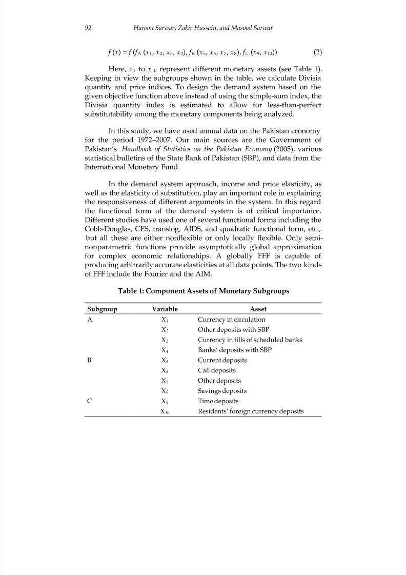
f (x) = f ( f A (x1, x2, x3, x4), f B (x5, x6, x7, x8), f C (x9, x10)) (2)

Here, x1 to x10 represent different monetary assets (see Table 1).Keeping in view the subgroups shown in the table, we calculate Divisiaquantity and price indices. To design the demand system based on thegiven objective function above instead of using the simple-sum index, theDivisia quantity index is estimated to allow for less-than-perfectsubstitutability among the monetary components being analyzed.

In this study, we have used annual data on the Pakistan economyfor the period 1972–2007. Our main sources are the Government of Pakistan’s Handbook of Statistics on the Pakistan Economy (2005), variousstatistical bulletins of the State Bank of Pakistan (SBP), and data from theInternational Monetary Fund.

In the demand system approach, income and price elasticity, aswell as the elasticity of substitution, play an important role in explaining

the responsiveness of different arguments in the system. In this regardthe functional form of the demand system is of critical importance.Different studies have used one of several functional forms including theCobb-Douglas, CES, translog, AIDS, and quadratic functional form, etc.,

but all these are either nonflexible or only locally flexible. Only semi-nonparametric functions provide asymptotically global approximationfor complex economic relationships. A globally FFF is capable of producing arbitrarily accurate elasticities at all data points. The two kindsof FFF include the Fourier and the AIM.

Table 1: Component Assets of Monetary Subgroups

Subgroup Variable Asset

A X 1 Currency in circulation

X 2 Other deposits with SBP

X3 Currency in tills of scheduled banks

X4 Banks’ deposits with SBP

B X5 Current deposits

X6 Call deposits

X7 Other deposits

X8 Savings deposits

C X9 Time depositsX10 Residents’ foreign currency deposits




3.1. AIM Specification

We use an AIM due to its established superiority over the Fourier.The AIM is relatively simple to use in economic analysis, while theFourier is more appropriate to engineering and physics. Moreover, anFFF in lower orders could violate the regularity conditions (Serletis, 2007).

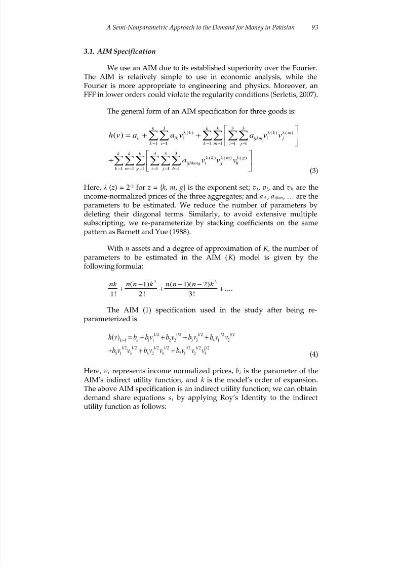
The general form of an AIM specification for three goods is:

3 3 3( ) ( ) ( )

1 1 1 1 1 1

3 3 3( ) ( ) ( )

1 1 1 1 1 1

( )k k k

k k m

o ik i ijkm i j

k i k m i j

k k k k m g

ijhkmg i j h

k m g i j h

h v a a v a v v

a v v v

λ λ λ

= = = = = =

λ λ λ

= = = = = =

= + +

+

∑∑ ∑∑ ∑∑

∑∑∑ ∑∑∑(3)

Here, λ (z) = 2-2 for z = {k , m, g} is the exponent set; vi, v j, and vh are the

income-normalized prices of the three aggregates; and a ik , aijkm, … are theparameters to be estimated. We reduce the number of parameters bydeleting their diagonal terms. Similarly, to avoid extensive multiplesubscripting, we re-parameterize by stacking coefficients on the samepattern as Barnett and Yue (1988).

With n assets and a degree of approximation of K , the number of parameters to be estimated in the AIM (K ) model is given by thefollowing formula:

2 3( 1) ( 1)( 2)

....1! 2! 3!

nk n n k n n n k − − −+ + +

The AIM (1) specification used in the study after being re-

parameterized is

1/2 1/2 1/2 1/2 1/2

1 1 1 2 2 3 3 4 1 2

1/2 1/2 1/2 1/2 1/2 1/2 1/2

5 1 3 6 2 3 7 1 2 3

( )k oh v b b v b v b v b v v

b v v b v v b v v v

== + + + +

+ + + (4)

Here, vi represents income normalized prices, bi is the parameter of theAIM’s indirect utility function, and k is the model’s order of expansion.The above AIM specification is an indirect utility function; we can obtain

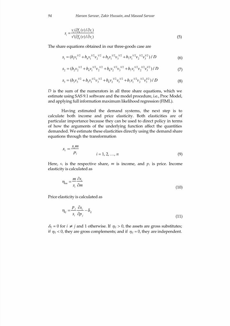
demand share equations s i by applying Roy’s Identity to the indirectutility function as follows:




(5)

The share equations obtained in our three-goods case are

1/ 2 1/ 2 1/ 2 1/ 2 1/ 2 1/ 2 1/ 2 1/ 2

1 1 1 4 1 2 5 1 3 7 1 2 3( ) / s b v b v v b v v b v v v D= + + + (6)

1/ 2 1/ 2 1/ 2 1/ 2 1/ 2 1/ 2 1/ 2 1/ 2

2 2 2 4 1 2 6 2 3 7 1 2 3( ) / s b v b v v b v v b v v v D= + + +

(7)

1/ 2 1/ 2 1/ 2 1/ 2 1/ 2 1/ 2 1/ 2 1/ 2

3 3 3 5 1 3 6 2 3 7 1 2 3( ) / s b v b v v b v v b v v v D= + + +

(8)

D is the sum of the numerators in all three share equations, which weestimate using SAS 9.1 software and the model procedure, i.e., Proc Model,and applying full information maximum likelihood regression (FIML).

Having estimated the demand systems, the next step is tocalculate both income and price elasticity. Both elasticities are of particular importance because they can be used to direct policy in termsof how the arguments of the underlying function affect the quantitiesdemanded. We estimate these elasticities directly using the demand shareequations through the transformation

ii

i

s m x

p=

i = 1, 2, …, n (9)

Here, si is the respective share, m is income, and p i is price. Incomeelasticity is calculated as

i

im

i

sm

s m

∂η =

∂ (10)

Price elasticity is calculated as

j iij ij

i j

p s

s p

∂η = − δ

∂(11)

δ ij= 0 for i

≠

j and 1 otherwise. If η ij

> 0, the assets are gross substitutes;if η ij < 0, they are gross complements; and if η ij = 0, they are independent.

( ( ) / )

( ( ) / )

i k ii

k i

v f v vs

v f v v

∂ ∂=

′ ∂ ∂




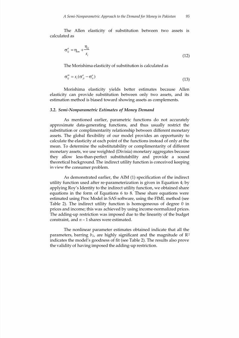
The Allen elasticity of substitution between two assets iscalculated as

ija

ij im

is

ησ = η +

(12)

The Morishima elasticity of substitution is calculated as

( )m a a

ij i ji iisσ = σ − σ(13)

Morishima elasticity yields better estimates because Allenelasticity can provide substitution between only two assets, and itsestimation method is biased toward showing assets as complements.

3.2. Semi-Nonparametric Estimates of Money Demand

As mentioned earlier, parametric functions do not accuratelyapproximate data-generating functions, and thus usually restrict thesubstitution or complimentarity relationship between different monetaryassets. The global flexibility of our model provides an opportunity tocalculate the elasticity at each point of the functions instead of only at themean. To determine the substitutability or complimentarity of differentmonetary assets, we use weighted (Divisia) monetary aggregates becausethey allow less-than-perfect substitutability and provide a soundtheoretical background. The indirect utility function is conceived keepingin view the consumer problem.

As demonstrated earlier, the AIM (1) specification of the indirectutility function used after re-parameterization is given in Equation 4; byapplying Roy’s Identity to the indirect utility function, we obtained shareequations in the form of Equations 6 to 8. These share equations wereestimated using Proc Model in SAS software, using the FIML method (seeTable 2). The indirect utility function is homogeneous of degree 0 inprices and income; this was achieved by using income-normalized prices.The adding-up restriction was imposed due to the linearity of the budgetconstraint, and n – 1 shares were estimated.

The nonlinear parameter estimates obtained indicate that all the

parameters, barring b2, are highly significant and the magnitude of R2

indicates the model’s goodness of fit (see Table 2). The results also provethe validity of having imposed the adding-up restriction.




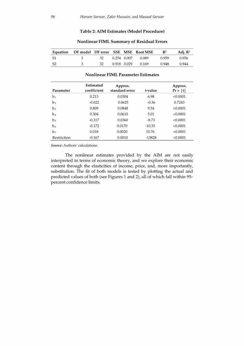
Table 2: AIM Estimates (Model Procedure)

Nonlinear FIML Summary of Residual Errors

Equation DF model DF error SSE MSE Root MSE R2 Adj. R2

S1 3 32 0.254 0.007 0.089 0.959 0.956

S2 3 32 0.918 0.029 0.169 0.948 0.944

Nonlinear FIML Parameter Estimates

Parameter

Estimated

coefficientApprox.

standard error t-valueApprox.Pr > |t|

b1 0.213 0.0304 6.98 <0.0001

b2 -0.022 0.0625 -0.36 0.7243

b3 0.809 0.0848 9.54 <0.0001

b4 0.304 0.0610 5.01 <0.0001

b5 -0.317 0.0360 -8.73 <0.0001 b6 -0.172 0.0170 -10.33 <0.0001

b7 0.018 0.0020 10.76 <0.0001

Restriction -0.167 0.0010 -13828 <0.0001

Source: Authors’ calculations.

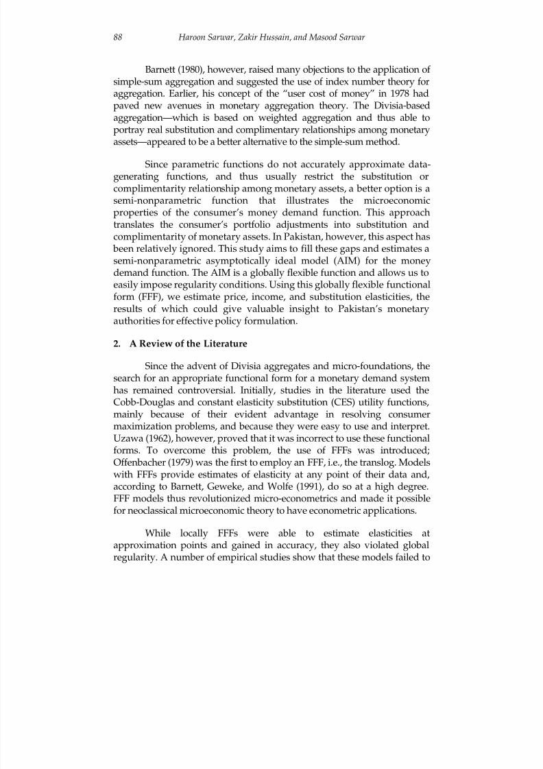
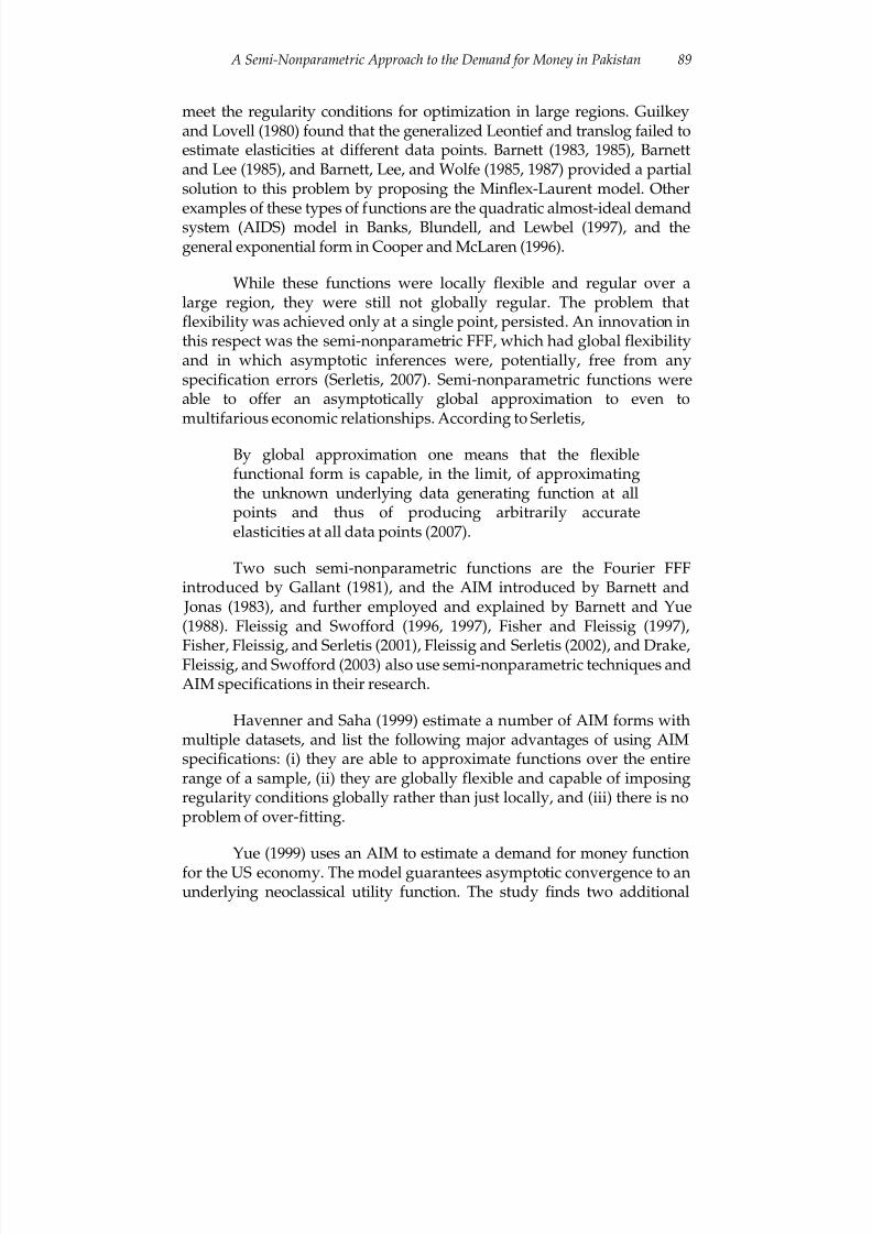
The nonlinear estimates provided by the AIM are not easilyinterpreted in terms of economic theory, and we explore their economiccontent through the elasticities of income, price, and, more importantly,substitution. The fit of both models is tested by plotting the actual andpredicted values of both (see Figures 1 and 2), all of which fall within 95-

percent confidence limits.




Figure 1: Predicted and Actual Values of Model S1

Figure 2: Predicted and Actual Values of Model S2

To calculate the elasticities, we compute derivatives of thedemand share equations and plug these into their respective elasticityformulae. Price elasticity (Eij) is calculated as

j iij ij

i j

p s E

s p

∂= − δ

∂

δ ij = 0 for i ≠ j and 1 otherwise. If Eij > 0, the assets are gross substitutes;if Eij < 0, they are gross complements; and if Eij = 0, they are independent.




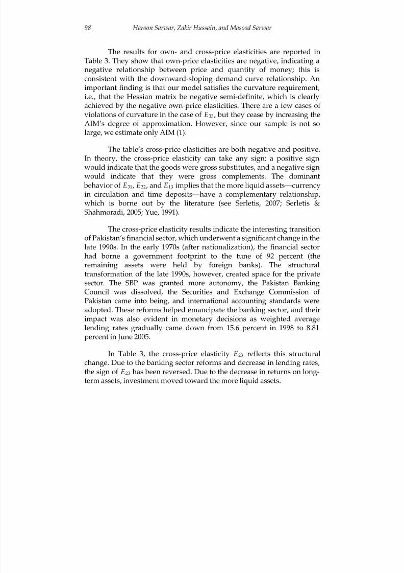
The results for own- and cross-price elasticities are reported inTable 3. They show that own-price elasticities are negative, indicating anegative relationship between price and quantity of money; this isconsistent with the downward-sloping demand curve relationship. Animportant finding is that our model satisfies the curvature requirement,

i.e., that the Hessian matrix be negative semi-definite, which is clearlyachieved by the negative own-price elasticities. There are a few cases of violations of curvature in the case of E33, but they cease by increasing theAIM’s degree of approximation. However, since our sample is not solarge, we estimate only AIM (1).

The table’s cross-price elasticities are both negative and positive.In theory, the cross-price elasticity can take any sign: a positive signwould indicate that the goods were gross substitutes, and a negative signwould indicate that they were gross complements. The dominant

behavior of E31, E32, and E13 implies that the more liquid assets—currencyin circulation and time deposits—have a complementary relationship,

which is borne out by the literature (see Serletis, 2007; Serletis &Shahmoradi, 2005; Yue, 1991).

The cross-price elasticity results indicate the interesting transitionof Pakistan’s financial sector, which underwent a significant change in thelate 1990s. In the early 1970s (after nationalization), the financial sectorhad borne a government footprint to the tune of 92 percent (theremaining assets were held by foreign banks). The structuraltransformation of the late 1990s, however, created space for the privatesector. The SBP was granted more autonomy, the Pakistan BankingCouncil was dissolved, the Securities and Exchange Commission of

Pakistan came into being, and international accounting standards wereadopted. These reforms helped emancipate the banking sector, and theirimpact was also evident in monetary decisions as weighted averagelending rates gradually came down from 15.6 percent in 1998 to 8.81percent in June 2005.

In Table 3, the cross-price elasticity E23 reflects this structuralchange. Due to the banking sector reforms and decrease in lending rates,the sign of E23 has been reversed. Due to the decrease in returns on long-term assets, investment moved toward the more liquid assets.




Table 3: Own- and Cross-Price Elasticities

Year E11 E22 E33 E12 E13 E21 E23 E31 E32

1973 -1.217 -2.760 1.462 -6.947 -4.088 -2.512 -0.155 2.047 2.616

1974 -1.467 -3.507 2.040 -10.067 -5.318 -3.569 -0.659 2.807 3.134

1975 -0.629 -1.184 0.554 -1.447 -1.557 -0.237 0.917 0.356 1.6951976 -0.608 -0.804 -0.157 0.335 0.003 0.668 1.102 -0.754 0.155

1977 -0.598 -0.993 0.345 -0.626 -0.878 0.099 0.744 -0.017 0.943

1978 -0.595 -0.787 -0.104 0.257 -0.096 0.572 0.886 -0.624 0.181

1979 -0.575 -0.855 -0.174 -0.196 -0.552 0.305 0.706 -0.257 0.575

1980 -0.561 -0.972 -0.608 -1.240 -1.472 -0.079 0.545 0.219 1.207

1981 -0.546 -0.771 -0.171 -0.123 -0.563 0.368 0.614 -0.317 0.463

1982 -0.545 -0.681 -0.084 0.361 -0.179 0.672 0.716 -0.716 0.015

1983 -0.588 -0.625 -0.412 0.696 0.183 1.007 0.730 -1.389 -0.877

1984 -0.498 -0.678 0.263 -0.192 -0.786 0.418 0.514 -0.329 0.477

1985 -0.550 -0.617 -0.263 0.644 0.024 0.856 0.649 -1.036 -0.435

1986 -0.549 -0.609 -0.283 0.700 0.039 0.936 0.678 -1.121 -0.5151987 -0.536 -0.591 -0.262 0.678 -0.006 0.848 0.565 -1.005 -0.456

1988 -0.459 -0.568 0.167 0.150 -0.715 0.635 0.475 -0.584 0.215

1989 -0.477 -0.549 0.028 0.391 -0.449 0.707 0.429 -0.676 -0.026

1990 -0.573 -0.568 -0.472 0.871 0.096 1.159 0.479 -1.704 -1.262

1991 -0.366 -0.372 0.199 0.380 -0.842 0.716 0.176 -0.627 -0.022

1992 -0.540 -0.532 -0.446 0.849 0.009 0.976 0.316 -1.320 -0.960

1993 -0.540 -0.525 -0.451 0.922 -0.002 1.020 0.283 -1.426 -1.031

1994 -0.515 -0.493 -0.431 0.882 -0.059 0.906 0.189 -1.192 -0.851

1995 -0.522 -0.488 -0.479 0.879 -0.092 0.887 0.113 -1.228 -0.916

1996 -0.554 -0.510 -0.562 0.846 -0.172 1.029 0.042 -1.645 -1.335

1997 -0.534 -0.486 -0.553 0.842 -0.201 0.919 -0.010 -1.425 -1.123

1998 -0.585 -0.521 -0.633 0.712 -0.407 1.078 -0.167 -2.176 -1.835

1999 -0.579 -0.515 -0.635 0.714 -0.422 1.052 -0.184 -2.139 -1.785

2000 -0.583 -0.507 -0.680 0.578 -0.721 0.994 -0.401 -2.291 -1.902

2001 -0.541 -0.475 -0.629 0.711 -0.415 0.763 -0.181 -1.372 -1.068

2002 -0.559 -0.487 -0.674 0.688 -0.697 0.883 -0.338 -1.838 -1.450

2003 -0.559 -0.487 -0.678 0.662 -0.727 0.855 -0.346 -1.769 -1.429

2004 -0.527 -0.455 -0.644 0.745 -0.509 0.682 -0.215 -1.225 -0.900

2005 -0.499 -0.418 -0.608 0.821 -0.409 0.609 -0.178 -1.011 -0.674

2006 -0.542 -0.469 -0.708 0.705 -1.103 0.978 -0.555 -1.926 -1.527

2007 -0.557 -0.479 -0.704 0.702 -1.013 0.919 -0.483 -1.986 -1.480





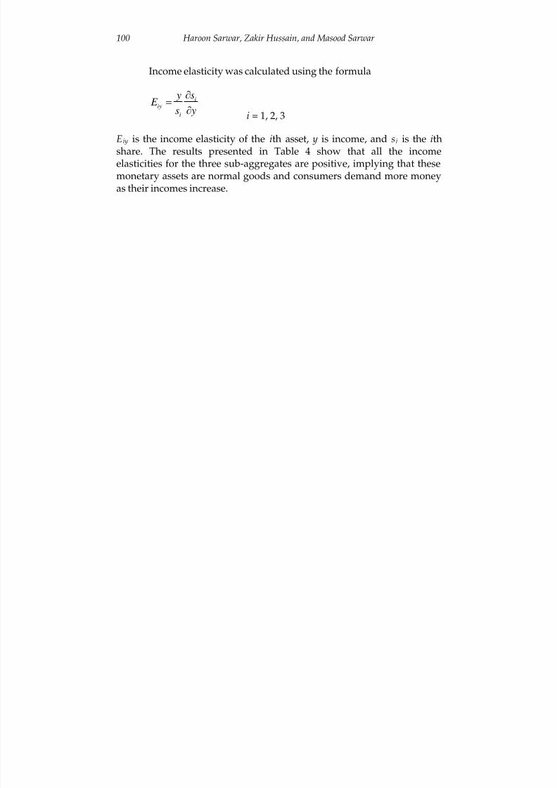
Income elasticity was calculated using the formula

iiy

i

s y E

s y

∂=

∂ i = 1, 2, 3

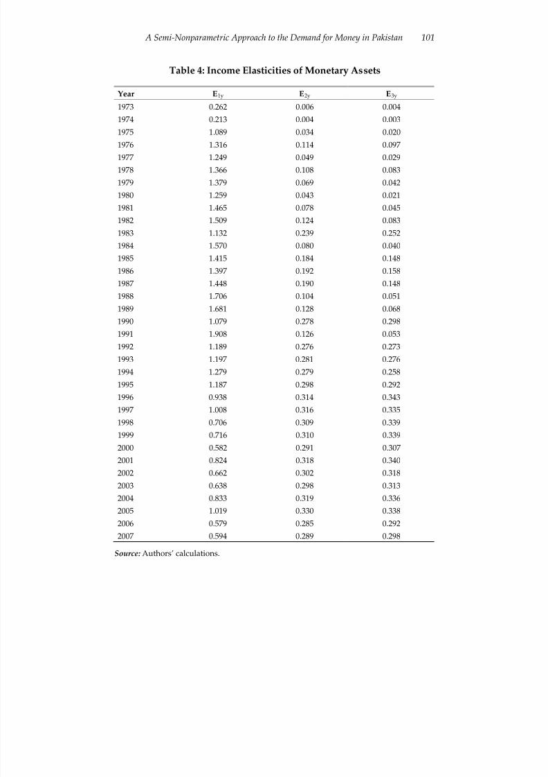
Eiy is the income elasticity of the ith asset, y is income, and si is the ithshare. The results presented in Table 4 show that all the incomeelasticities for the three sub-aggregates are positive, implying that thesemonetary assets are normal goods and consumers demand more moneyas their incomes increase.




Table 4: Income Elasticities of Monetary Assets

Year E1y E2y E3y

1973 0.262 0.006 0.004

1974 0.213 0.004 0.003

1975 1.089 0.034 0.0201976 1.316 0.114 0.097

1977 1.249 0.049 0.029

1978 1.366 0.108 0.083

1979 1.379 0.069 0.042

1980 1.259 0.043 0.021

1981 1.465 0.078 0.045

1982 1.509 0.124 0.083

1983 1.132 0.239 0.252

1984 1.570 0.080 0.040

1985 1.415 0.184 0.148

1986 1.397 0.192 0.1581987 1.448 0.190 0.148

1988 1.706 0.104 0.051

1989 1.681 0.128 0.068

1990 1.079 0.278 0.298

1991 1.908 0.126 0.053

1992 1.189 0.276 0.273

1993 1.197 0.281 0.276

1994 1.279 0.279 0.258

1995 1.187 0.298 0.292

1996 0.938 0.314 0.343

1997 1.008 0.316 0.335

1998 0.706 0.309 0.339

1999 0.716 0.310 0.339

2000 0.582 0.291 0.307

2001 0.824 0.318 0.340

2002 0.662 0.302 0.318

2003 0.638 0.298 0.313

2004 0.833 0.319 0.336

2005 1.019 0.330 0.338

2006 0.579 0.285 0.292

2007 0.594 0.289 0.298





This finding is consistent with previous studies (Akhtar, 1994;Khan, 1994), and implies that, as per capita income rises, the demand formoney increases since the income elasticity is positive. Over time, thedecrease in income elasticity of reserve money indicates that, withfinancial developments such as debit and credit cards, and ATMs, etc.,

the extent of preference for cash has diminished. On the other hand, theincreasing magnitude of income elasticities for narrow and broadaggregates shows that the demand for these assets rises as incomesincrease (see Table 4).

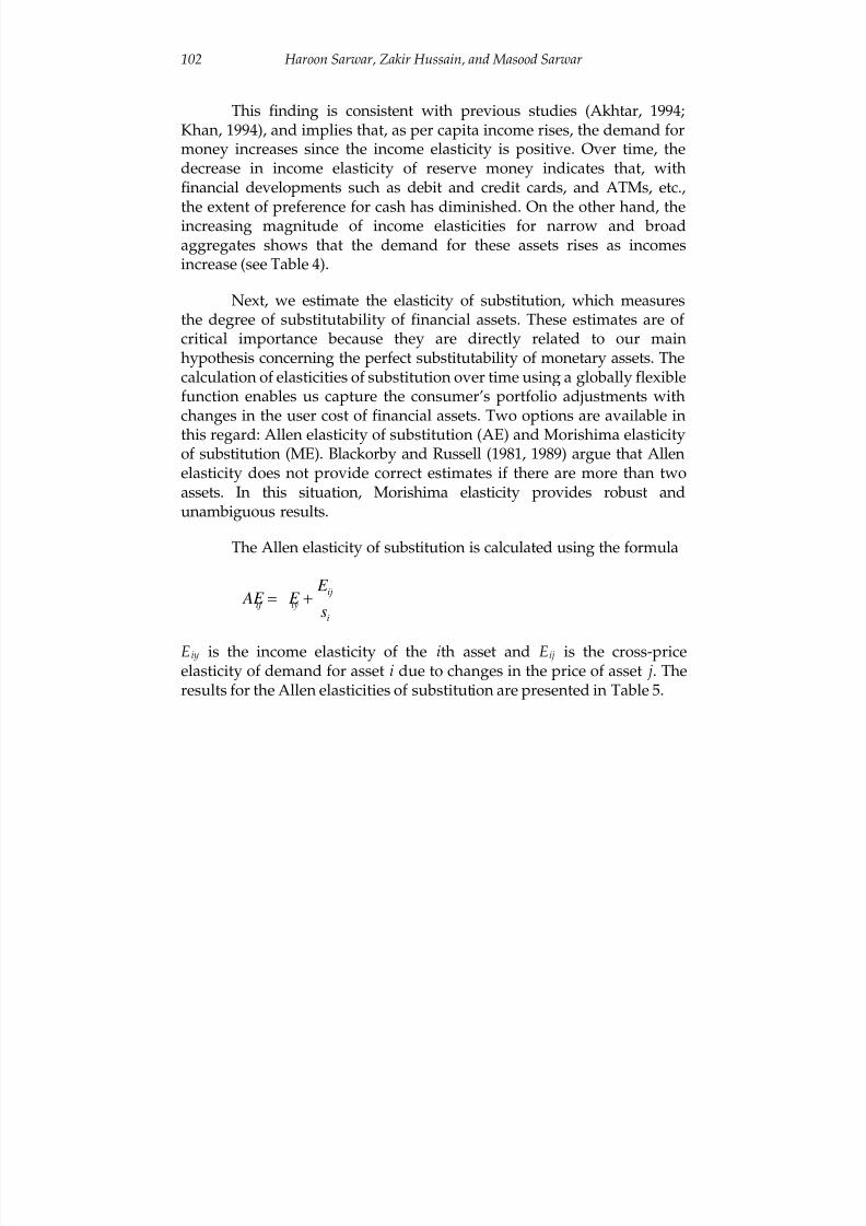
Next, we estimate the elasticity of substitution, which measuresthe degree of substitutability of financial assets. These estimates are of critical importance because they are directly related to our mainhypothesis concerning the perfect substitutability of monetary assets. Thecalculation of elasticities of substitution over time using a globally flexiblefunction enables us capture the consumer’s portfolio adjustments withchanges in the user cost of financial assets. Two options are available in

this regard: Allen elasticity of substitution (AE) and Morishima elasticityof substitution (ME). Blackorby and Russell (1981, 1989) argue that Allenelasticity does not provide correct estimates if there are more than twoassets. In this situation, Morishima elasticity provides robust andunambiguous results.

The Allen elasticity of substitution is calculated using the formula

ij

ij iy

i

E AE E

s= +

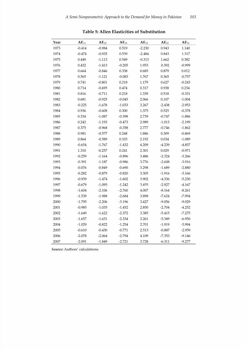
Eiy is the income elasticity of the ith asset and Eij is the cross-priceelasticity of demand for asset i due to changes in the price of asset j. Theresults for the Allen elasticities of substitution are presented in Table 5.




Table 5: Allen Elasticities of Substitution

Year AE11 AE22 AE33 AE12 AE32 AE31

1973 -0.414 -0.984 0.519 -2.230 0.943 1.140

1974 -0.474 -0.935 0.539 -2.484 0.843 1.317

1975 0.449 -1.113 0.549 -0.313 1.662 0.3821976 0.432 -1.413 -0.205 1.953 0.392 -0.999

1977 0.664 -0.846 0.338 0.685 0.879 0.012

1978 0.565 -1.121 -0.083 1.767 0.365 -0.757

1979 0.741 -0.801 0.218 1.179 0.627 -0.243

1980 0.714 -0.695 0.474 0.317 0.938 0.234

1981 0.816 -0.711 0.218 1.339 0.518 -0.331

1982 0.681 -0.925 -0.045 2.066 0.107 -1.004

1983 -0.225 -1.678 -1.033 3.267 -2.438 -2.953

1984 0.936 -0.608 0.300 1.375 0.525 -0.378

1985 0.334 -1.087 -0.398 2.739 -0.747 -1.886

1986 0.242 -1.193 -0.473 2.989 -1.013 -2.1991987 0.375 -0.968 -0.358 2.777 -0.746 -1.862

1988 0.981 -0.577 0.248 1.886 0.309 -0.869

1989 0.864 -0.589 0.103 2.192 0.034 -1.089

1990 -0.654 -1.767 -1.432 4.209 -4.239 -4.857

1991 1.310 -0.257 0.241 2.301 0.029 -0.971

1992 -0.259 -1.164 -0.896 3.486 -2.324 -3.266

1993 -0.391 -1.187 -0.986 3.776 -2.608 -3.916

1994 -0.076 -0.849 -0.690 3.298 -1.689 -2.880

1995 -0.282 -0.879 -0.820 3.305 -1.916 -3.166

1996 -0.939 -1.474 -1.602 3.902 -4.336 -5.230

1997 -0.679 -1.095 -1.242 3.455 -2.927 -4.167

1998 -1.604 -2.106 -2.760 4.007 -8.164 -8.261

1999 -1.539 -1.988 -2.684 3.898 -7.624 -7.994

2000 -1.795 -2.206 -3.196 3.427 -9.056 -9.029

2001 -0.985 -1.035 -1.452 2.850 -2.704 -4.252

2002 -1.649 -1.622 -2.372 3.385 -5.415 -7.275

2003 -1.657 -1.631 -2.334 3.261 -5.349 -6.950

2004 -1.029 -0.822 -1.254 2.701 -1.919 -3.994

2005 -0.610 -0.430 -0.771 2.513 -0.887 -2.959

2006 -2.078 -2.064 -2.794 4.109 -7.353 -9.146

2007 -2.091 -1.849 -2.721 3.728 -6.311 -9.277





The dominant pattern assumed by the estimates of Allen own-substitution elasticity is negative, as expected. But the remaining threeAllen elasticities are not deemed reliable due to their inherent drawbackas pointed out by Blackorby and Russell (1981, 1989). To overcome this,we use Morishima elasticity, which is calculated as

( )ij i ji ii

ME s AE AE = −

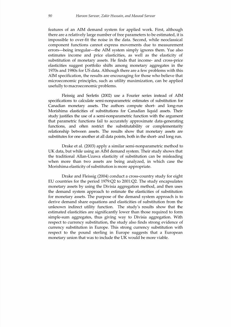
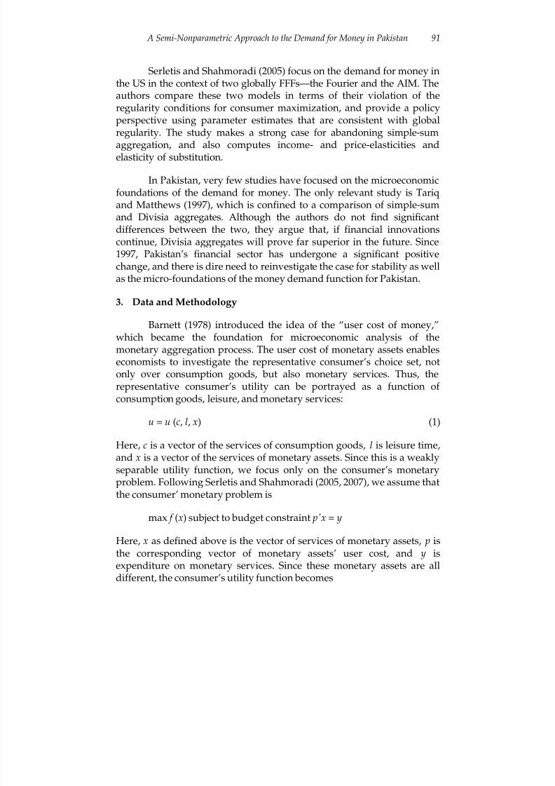
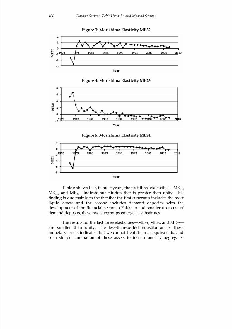
Here, si is the share of the ith asset. Estimates for the Morishimaelasticities of substitution are shown in Table 6 and Figures 3 to 5.




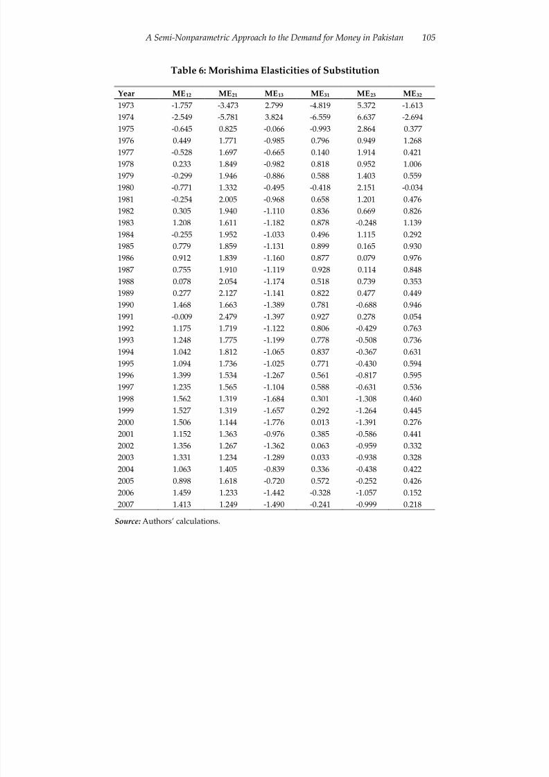
Table 6: Morishima Elasticities of Substitution

Year ME12 ME21 ME13 ME31 ME23 ME32

1973 -1.757 -3.473 2.799 -4.819 5.372 -1.613

1974 -2.549 -5.781 3.824 -6.559 6.637 -2.694

1975 -0.645 0.825 -0.066 -0.993 2.864 0.377

1976 0.449 1.771 -0.985 0.796 0.949 1.268

1977 -0.528 1.697 -0.665 0.140 1.914 0.421

1978 0.233 1.849 -0.982 0.818 0.952 1.006

1979 -0.299 1.946 -0.886 0.588 1.403 0.559

1980 -0.771 1.332 -0.495 -0.418 2.151 -0.034

1981 -0.254 2.005 -0.968 0.658 1.201 0.476

1982 0.305 1.940 -1.110 0.836 0.669 0.826

1983 1.208 1.611 -1.182 0.878 -0.248 1.139

1984 -0.255 1.952 -1.033 0.496 1.115 0.292

1985 0.779 1.859 -1.131 0.899 0.165 0.930

1986 0.912 1.839 -1.160 0.877 0.079 0.976

1987 0.755 1.910 -1.119 0.928 0.114 0.8481988 0.078 2.054 -1.174 0.518 0.739 0.353

1989 0.277 2.127 -1.141 0.822 0.477 0.449

1990 1.468 1.663 -1.389 0.781 -0.688 0.946

1991 -0.009 2.479 -1.397 0.927 0.278 0.054

1992 1.175 1.719 -1.122 0.806 -0.429 0.763

1993 1.248 1.775 -1.199 0.778 -0.508 0.736

1994 1.042 1.812 -1.065 0.837 -0.367 0.631

1995 1.094 1.736 -1.025 0.771 -0.430 0.594

1996 1.399 1.534 -1.267 0.561 -0.817 0.595

1997 1.235 1.565 -1.104 0.588 -0.631 0.536

1998 1.562 1.319 -1.684 0.301 -1.308 0.460

1999 1.527 1.319 -1.657 0.292 -1.264 0.445

2000 1.506 1.144 -1.776 0.013 -1.391 0.276

2001 1.152 1.363 -0.976 0.385 -0.586 0.441

2002 1.356 1.267 -1.362 0.063 -0.959 0.332

2003 1.331 1.234 -1.289 0.033 -0.938 0.328

2004 1.063 1.405 -0.839 0.336 -0.438 0.422

2005 0.898 1.618 -0.720 0.572 -0.252 0.426

2006 1.459 1.233 -1.442 -0.328 -1.057 0.152

2007 1.413 1.249 -1.490 -0.241 -0.999 0.218





Figure 3: Morishima Elasticity ME32



Table 6 shows that, in most years, the first three elasticities—ME12,ME21, and ME13—indicate substitution that is greater than unity. Thisfinding is due mainly to the fact that the first subgroup includes the mostliquid assets and the second includes demand deposits; with thedevelopment of the financial sector in Pakistan and smaller user cost of demand deposits, these two subgroups emerge as substitutes.

The results for the last three elasticities—ME23, ME13, and ME32—are smaller than unity. The less-than-perfect substitution of thesemonetary assets indicates that we cannot treat them as equivalents, andso a simple summation of these assets to form monetary aggregates




would be misleading. It also indicates that weighted aggregates are a better option for monetary aggregation. This result supports our mainhypothesis that all monetary assets are not perfect substitutes for oneanother, as simple-sum aggregation might otherwise imply.

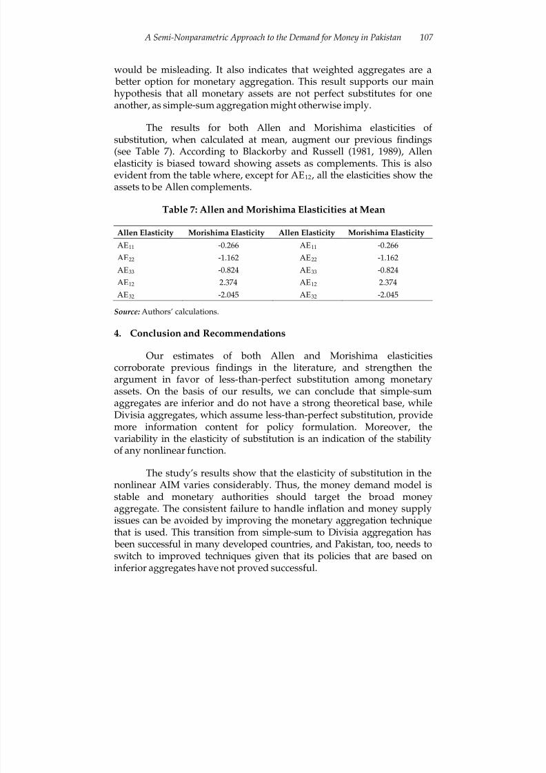
The results for both Allen and Morishima elasticities of substitution, when calculated at mean, augment our previous findings(see Table 7). According to Blackorby and Russell (1981, 1989), Allenelasticity is biased toward showing assets as complements. This is alsoevident from the table where, except for AE12, all the elasticities show theassets to be Allen complements.

Table 7: Allen and Morishima Elasticities at Mean

Allen Elasticity Morishima Elasticity Allen Elasticity Morishima Elasticity

AE11 -0.266 AE11 -0.266

AE22 -1.162 AE22 -1.162

AE33 -0.824 AE33 -0.824AE12 2.374 AE12 2.374

AE32 -2.045 AE32 -2.045


4. Conclusion and Recommendations

Our estimates of both Allen and Morishima elasticitiescorroborate previous findings in the literature, and strengthen theargument in favor of less-than-perfect substitution among monetaryassets. On the basis of our results, we can conclude that simple-sum

aggregates are inferior and do not have a strong theoretical base, whileDivisia aggregates, which assume less-than-perfect substitution, providemore information content for policy formulation. Moreover, thevariability in the elasticity of substitution is an indication of the stabilityof any nonlinear function.

The study’s results show that the elasticity of substitution in thenonlinear AIM varies considerably. Thus, the money demand model isstable and monetary authorities should target the broad moneyaggregate. The consistent failure to handle inflation and money supplyissues can be avoided by improving the monetary aggregation techniquethat is used. This transition from simple-sum to Divisia aggregation has

been successful in many developed countries, and Pakistan, too, needs toswitch to improved techniques given that its policies that are based oninferior aggregates have not proved successful.




References

Akhtar, H. (1994). The search for a stable money demand function for Pakistan: An application of the method of cointegration. Paper presented at the10th annual general meeting of the Pakistan Society of Development Economists, Islamabad.

Banks, J., Blundell, R., & Lewbel, A. (1997). Quadratic Engel curves andconsumer demand. Review of Economics and Statistics, 79, 527–539.

Barnett, W. A. (1978). The user cost of money. Economics Letters, 1, 145–149.

Barnett, W. A. (1980). Economic monetary aggregates: An application of aggregation and index number theory. Journal of Econometrics, 14,11–48.

Barnett, W. A. (1983a). New indices of money supply and the flexibleLaurent demand system. Journal of Business and Economic Statistics,

1, 7–23.

Barnett, W. A. (1983b). Definitions of second-order approximation and of flexible functional form. Economics Letters, 12, 31–35.

Barnett, W. A. (1985). The Minflex-Laurent translog flexible functionalform. Journal of Econometrics, 30, 33–44.

Barnett, W. A., & Jonas, A. (1983). The Müntz-Szátz demand system: Anapplication of a globally well behaved series expansion. EconomicsLetters, 11, 337–342.

Barnett, W. A., & Lee, Y. W. (1985). The global properties of the Minflex-Laurent, generalized Leontief, and translog flexible functionalforms. Econometrica, 53, 1421–1437.

Barnett, W. A., Geweke, J., & Wolfe, M. D. (1991). Semi-nonparametricBayesian estimation of the asymptotically ideal production model. Journal of Econometrics, 49, 5–50.

Barnett, W. A., Lee, Y. W., & Wolfe, M. D. (1985). The three-dimensionalglobal properties of the Minflex-Laurent, generalized Leontief,and translog flexible functional forms. Journal of Econometrics, 30,3–31.




Barnett, W.A., Lee, Y.W., & Wolfe, M. D. (1987). The global properties of the two Minflex-Laurent flexible functional forms. Journal of Econometrics, 36, 281–298.

Barnett, W. A., & Yue, P. (1988). Semi-nonparametric estimation of theasymptotically ideal model: The AIM demand system. In G. F.Rhodes & T. B. Fomby (Eds.), Nonparametric and robust inference, Advances in Econometrics (7, 229–251). Greenwich, CT: JAI Press.

Blackorby, C., & Russell, R.R. (1981). The Morishima elasticity of substitution, symmetry, constancy, separability, and itsrelationship to the Hicks and Allen elasticities. Review of EconomicStudies, 48, 147–158.

Blackorby, C., & Russell, R. R. (1989). Will the real elasticity of substitutionplease stand up? American Economic Review, 79, 882–888.

Chetty, V.K. (1969). On measuring the nearness of near-moneys. AmericanEconomic Review, 59, 270–281.

Cooper, R.J., & McLaren, K.R. (1996). A system of demand equationssatisfying effectively global regularity conditions. Review of Economics and Statistics, 78, 359–364.

Drake, L., & Fleissig, A.R. (2004). Semi-nonparametric estimates of currency substitution: The demand for sterling in Europe. Reviewof International Economics, 12, 374–394.

Drake, L., Fleissig, A.R., & Swofford, J. L. (2003). A semi-nonparametricapproach to the demand for UK monetary assets. Economica, 70,99–120.

Fisher, D., & Fleissig, A.R. (1997). Monetary aggregation and the demand forassets. Journal of Money, Credit, and Banking, 29, 458–475.

Fisher, D., Fleissig, A.R., & Serletis, A. (2001). An empirical comparison of flexible demand system functional forms. Journal of AppliedEconometrics, 16, 59–80.

Fleissig, A.R., & Serletis, A. (2002). Semi-nonparametric estimates of substitution for Canadian monetary assets. Canadian Journal of Economics, 35, 78–91.




Fleissig, A.R., & Swofford, J.L. (1996). A dynamic asymptotically idealmodel of money demand. Journal of Monetary Economics, 37, 371–380.

Fleissig, A.R., & Swofford, J L. (1997). Dynamic asymptotically idealmodels and finite approximation. Journal of Business and Economic

Statistics, 15, 482–492.

Gallant, A. R. (1981). On the bias in flexible functional forms and anessentially unbiased form: The Fourier flexible form. Journal of Econometrics, 15, 211–245.

Guilkey, D. K., & Lovell, C. A. K. (1980). On the flexibility of the translogapproximation. International Economic Review, 21, 137–147.

Havenner, A., & Saha, A. (1999). Globally flexible asymptotically idealmodels. American Journal of Agricultural Economics, 81, 703–710.

Khan, A. H. (1994). Financial liberalization and the demand for money inPakistan. Paper presented at the 10th annual general meeting of thePakistan Society of Development Economists, Islamabad.

Offenbacher, E. K. (1979). The substitution of monetary assets. (Doctoraldissertation, University of Chicago, IL).

Serletis, A. (2007). The demand for money: Theoretical and empirical approaches (2nd ed.). New York, NY: Springer.

Serletis, A., & Shahmoradi, A. (2005). Semi-nonparametric estimates of the demand for money in the United States. Macroeconomic

Dynamics, 9, 542–559.Serletis, A., & Shahmoradi, A. (2007). Flexible functional forms, curvature

conditions, and the demand for assets. Macroeconomic Dynamics,11(4), 455–486.

Tariq, S. M., & Matthews, K. (1997). The demand for simple-sum andDivisia monetary aggregates for Pakistan: A cointegrationapproach. Pakistan Development Review, 36(3), 275–291.

Uzawa, H. (1962). Production functions with constant elasticities of substitution. Review of Economic Studies, 29, 291–299.

Yue, P. (1999). A microeconomic approach to estimating money demand: Theasymptotically ideal model. St. Louis, MO: Federal Reserve Bank of St. Louis.

Semi Non Parametric DMF 2011

Documents

Transcript of Semi Non Parametric DMF 2011