Supplanting the ‘Minnesota’ prior Forecasting...

ELSEVIER Journal of Monetary Economics 34 (1994) 4977510

JOURNALOF Monetary ECONOMICS

Supplanting the ‘Minnesota’ prior Forecasting macroeconomic time series using

real business cycle model priors

Beth F. Ingram, Charles H. Whiteman*

Depurtment of Economics, Unioersity of lowu. Iowa City. IA 52242, USA

(Received February 1993; final version received May 1994)

Abstract

Although general equilibrium models are in wide use in the theoretical macroeconomic literature, their empirical relevance is uncertain. We develop procedures for using dynamic general equilibrium models to aid in analyzing the observed time series relationships among macroeconomic variables. Our strategy is based on that developed by Doan. Litterman, and Sims (1984). who constructed a procedure for improving time series forecasts by shrinking vector autoregression coefficient estimates toward a prior view that vector time series are well-described as collections of independent random walks. In our case, the prior is derived from a fully-specified general equilibrium model. We demonstrate that, like the atheoretical random-walk priors, real business cycle model priors can aid in forecasting.

Kqv words: Forecasting; Business cycles; Bayesian VARs

JEL class~fificution: E37; Cl 1

*Corresponding author

We thank Chris Neely for excellent research assistance. We gratefully acknowledge the comments of an anonymous referee. Whiteman thanks the Institute for Empirical Macroeconomics at the Federal Reserve Bank of Minneapolis for support during work on this paper. The views expressed herein are

those of the authors and not necessarily those of the Federal Reserve Bank of Minneapolis or the

Federal Reserve System.

0304-3932/94/$07.00 ITI 1994 Elsevier Science B.V. All rights reserved

SSDI 030439329401168 A

498 B.F. Ingram, C.H. Whitman / Journal of‘Monetay Economics 34 (1994) 497-510

1. Introduction

Although the general equilibrium paradigm revolutionized macroeconomic thought, it has received little empirical support ~ statistical tests of models have generally led to rejections. The profession has formulated three responses to this empirical failure. The first is simply to dismiss formal statistical tests of fit. This approach, which has been pursued in the real business cycle literature, is founded in the belief that one can learn about the economy by fitting misspeci- fied models to the data - either by informal ‘calibration’ methods (e.g., Kydland and Prescott, 1982; Hansen, 1985) or by formal econometric methods (e.g., Altug, 1989; McGrattan. 1992; Braun, 1992). A second reaction is to abandon theoretical models and to concentrate on reduced-form models such as vector autoregressions (VARs), as pioneered by Sims (1980) and Litterman (1984). Though widely used in quantitative forecasting. this line of research has made only modest attempts to connect the reduced-form models to structural models formulated in the theoretical literature.’ The third strategy is to concentrate on a subset of implications of a theoretical model and to neglect troublesome features of the model and the data.

We believe that none of these reactions is entirely satisfactory and that theoretical models should play an important role in analyzing and forecasting economic time series. In this paper, we develop methods for loosening the straightjacket of theory without shedding it completely.

Our strategy is to use theory to aid in analyzing the time series relationships among macroeconomic variables as summarized in a VAR. Since unrestricted VARs produce large standard errors, following Doan. Litterman, and Sims (1984), it has become common practice to add to the sample some nonsample prior information about the VAR. Their ‘Minnesota’ prior is that the vector time series is well-described as a collection of independent random walks. The prior was derived from knowledge about the univariate behavior of macroeconomic time series, not from a particular theoretical macroeconomic model. The prior is generally used in a pseudo-Bayesian, mixed estimation procedure to generate a tractable model which produces better out-of-sample forecasts than the unrestricted VAR or naive models. We adopt this philosophy of combining prior information with the likelihood as represented by the VAR. However, our information is derived from a fully-specified general equilibrium model, allowing us to tie forecasting performance to specific features of the model.

Specifically, we formulate a structural model which depends on a parameter vector p. We have information - a prior distribution - for p. Associated with each setting of ~1 is an equilibrium law of motion for the economy. We determine

‘For exceptions, see Blanchard and Quah (1989). Sims (1986). and Leeper and Gordon (1992).

B.F. Ingram, C.H. Whiteman / Journal of Monetar?, Economics 34 (1994) 497-510 499

the implications this carries for the VAR representation of the model, and use the mapping from p to model VAR to induce a prior distribution on VAR coefficients which can be combined with sample information. By varying a scale factor associated with the prior variance, we are able to adjust the weight given to the prior - the theoretical model - in the estimation.

The model of interest here is the real business cycle (RBC) model described in King, Plosser, and Rebel0 (1988). It is known from other studies that this model fails to fit the data along several dimensions: although it captures the persistence of the relevant subset of macroeconomic variables, it fails to mimic many of the correlations among the variables. Yet we show that even this simple theoretical model can improve the forecasting performance of an unrestricted VAR. Addi- tionally, we demonstrate that a prior derived from theory which was not designed for forecasting actually does about as well as one - the Minnesota prior ~ specifically designed to do so.

2. General approach

In spirit we follow Doan, Litterman, and Sims (1984) in first specifying a model for the data in the form of a density p( y 1 v) for the data, y, conditional on a set of parameters v called ‘coefficients’. Prior views about \J are specified via a density rc(\lI p) for \I conditional upon a set of hyperparameters ,LL. For Doan, Litterman, and Sims, the prior n(v1.) embodied the independent random walks notion. In our implementation, rc(\lIp) describes the implications carried for a VAR by a stochastic. dynamic general equilibrium model indexed by parameters ~1 which are meaningful from the point of view of economic theory.2 In either case, the joint density for the data and the parameters of interest is given

by P(Y~~~)~(~~~P).

Doan, Litterman, and Sims investigated the joint density of the data and the parameters of interest by numerically integrating p( y I V)TC( v I p) with respect to 11 to obtain a marginal distribution m( y I p). They referred to m( !: 1 p) informally as a ‘likelihood’ function, though they note that it is really a Bayesian notion, as it involves viewing the parameters 1’ as random. In their empirical example, Doan. Litterman, and Sims proceeded to conduct a simple search over p values to find high values of m(y I p). Thus their procedure has an informal interpretation as ‘maximizing’ the ‘likelihood’ function m( !: I p).

The Bayesian interpretation of related procedures has been made formal in recent work by Kwan (1990a. b) and Kim (1991). Both Kwan and Kim are concerned with limited-information Bayesian analysis - based not on the

*Thus 1’ for ‘VAR.. p for ‘model’

500 B.F. Ingram, C.H. Whiteman / Journal of MonetaT Economics 34 (1994) 497-510

likelihood function, but rather upon a set of statistics. A VAR suggests a natural set of statistics: the coefficient and error covariance estimates.

Thus our procedures have a limited-information Bayesian interpretation, with VAR estimates playing the role of the likelihood function in the standard full-information Bayesian approach. We adopt this limited-information Bayesian procedure primarily for computational convenience - we will hence- forth be concerned with evaluating ‘real time’ forecasting performance, which requires repeated re-estimation of models. In addition, we also adopt another Doan, Litterman, and Sims convenience, of avoiding joint system methods, and so we implement only equation-by-equation procedures.

Upon combining the partial likelihood with the prior distribution to be spelled out in the next section, we shall be concerned with the forecasting performance of the resulting model. Formally, this amounts to using the partial posterior together with conditional predictive densities to obtain unconditional predictive densities, and using them to interpret subsequently realized data. In particular, we will make formal the informal numerical integration of Doan, Litterman, and Sims by explicit specification of marginal prior distributions for p, though our investigation will ultimately be similar to theirs since we investi- gate the behavior of forecasting accuracy as a function of the shape and location parameters of the marginal prior.

3. The King, Plosser, and Rebel0 model

A representative, infinitely-lived agent has preferences over consumption, C,, and labor, h,, given by

EO tEl B’iWC,) + ln(l - k)].

The single good in the economy is produced according to

r, = A$: _“(h,X,)“,

where K represents the stock of capital, h the number of hours of labor supplied, X labor-augmenting technical progress, and A a technology shock that satisfies

ln.4, = pln A,_ r + sat, .!?A, - N(0, a’).

Capital evolves according to the following law of motion:

K t+ I = (1 - S)K, + I,,

where I represents investment and 6 represents depreciation. The sum of labor hours and leisure is constrained to be less than or equal to one, and consumption plus investment must not exceed total output. We assume that X, is growing

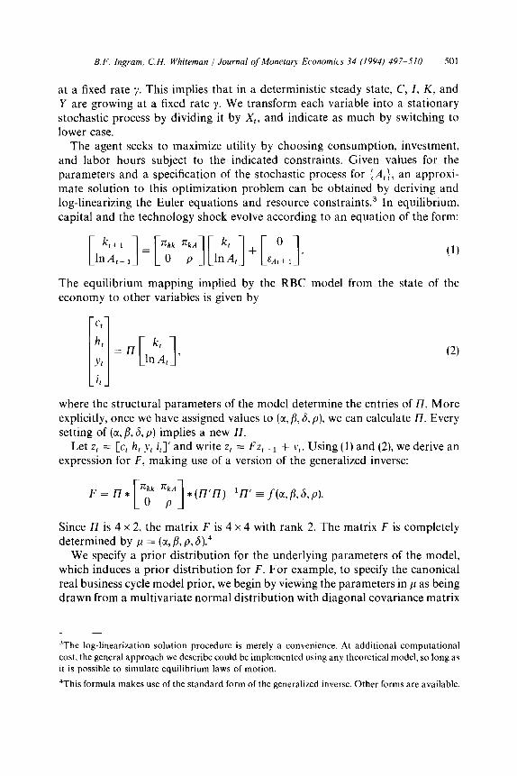
B.F. Ingram, C.H. Whiteman J Journal of Monetary Economics 34 (1994) 497-510 501

at a fixed rate 7. This implies that in a deterministic steady state, C, I, K, and Y are growing at a fixed rate y. We transform each variable into a stationary stochastic process by dividing it by X,, and indicate as much by switching to lower case.

The agent seeks to maximize utility by choosing consumption, investment, and labor hours subject to the indicated constraints. Given values for the parameters and a specification of the stochastic process for (A,), an approximate solution to this optimization problem can be obtained by deriving and log-linearizing the Euler equations and resource constraints3 In equilibrium, capital and the technology shock evolve according to an equation of the form:

(1)

The equilibrium mapping implied by the RBC model from the state of the economy to other variables is given by

where the structural parameters of the model determine the entries of I7. More explicitly, once we have assigned values to (a, fl, 6, p), we can calculate H. Every setting of (a, fl, 6, p) implies a new I7.

Let Z, = [c, h, yt i,]’ and write z, = Fz,- 1 + vf. Using (1) and (2), we derive an expression for F, making use of a version of the generalized inverse:

Since II is 4 x 2, the matrix F is 4 x 4 with rank 2. The matrix F is completely determined by p = (tl, /I, p, S).4

We specify a prior distribution for the underlying parameters of the model, which induces a prior distribution for F. For example, to specify the canonical real business cycle model prior, we begin by viewing the parameters in p as being drawn from a multivariate normal distribution with diagonal covariance matrix

jThe log-linearization solution procedure is merely a convenience. At additional computational

cost. the general approach we describe could be implemented using any theoretical model, so long as it is possible to simulate equilibrium laws of motion.

4This formula makes use of the standard form of the generalized inverse. Other forms are available.

for ~1. The moments are given by

0 0

0.0005 0 0 it = (x,&&p) -N

. 0.00004 0

0 0.00015

We calculate the induced prior for F by using a first-order Taylor expansion of F about the mean of p. Our approximate F is then normally distributed with mean f( ,G) and variance Vf( ji) * var( /I) * Vf(ji)‘. Specifically, given the prior specified above, our prior for F has mean given by

i

0.19 0.33 0.13 -0.02

0.45 0.67 0.29 -0.10

F= 1 . 0.49 1.32 0.40 0.17

1.35 4.00 1.18 0.64

This implies the following correlation matrix for the vector z,:

1.0

0.310 1.0 corr(z,,:,) = i

0.990 0.170 1.0 1 ,

LO.988 0.163 0.99997 1.01

and the following serial correlation matrix:

0.9931 0.2046 0.9983 0.9980 1 Under this prior, consumption, output, and investment are highly correlated with each other. In comparison, the correlation between hours and each of the other three series is quite small. Each of the series is highly serially correlated;

1

0.9949 0.3356 0.9802 0.9787

0.2470 0.9020 0.1197 0.1126 corr( z,,+,) =

0.9938 0.2117 0.9980 0.9976

however, hours displays the least amount of serial correlation. The vector autoregression for the ith component of a, can be

Zir = HirZ,_1 + Hi2Zt-2 + “’ + Hi6=1_6 + ~ + dit + ~;t,

c = 1, . . . ,T, i = 1, . . . ,4.

written as

B.F. Ingram, C.H. Whiteman J Journal qf Monetary Economics 34 (1994) 497-510 503

Let Zi denote the T x 1 vector of observations on Zit, and let X denote the T x 26 matrix consisting of observations on z, 1, . , zI b, constant, and trend. Then the system can be written in compact form as

Zi = XBi + ei, i=l ) . . . ,4.

We assume that ei is normally distributed with mean zero and variance of. Our estimation procedure involves combining the normal likelihood function

with the normal (induced) prior to obtain the posterior distribution, and then taking the posterior mean. Specifically, we take the elements of Bi corresponding to first lags to have prior mean given by the mean of the associated row of F. Other elements of Bi have prior means of zero. The prior covariance matrix for first lag coefficients is given by the covariance matrix for the corresponding row of F; covariance matrices for higher lag coefficients are proportional, with a proportionality parameter which shrinks harmonically with lag length. For example, letting B, denote the prior mean for Bi and Q1 its prior covariance matrix, we have for the mixed estimate of B L5

B, = [X’X/af + !2 1 l/t] l (x’z,/a: + 52; l&/t). (3)

The parameter t determines how much weight is given to the underlying structural model and 0 is the standard error of the residual from the first equation. As r grows, & approaches the unrestricted estimate of B1.

The parameters of the prior distributions for ,u = [a, fi, p, S] constitute the hyperparameters of the system under study. By varying these parameters and r, it is possible to influence the forecasting ability of the mixed system. Our measure of forecast performance is the In determinant of the error covariance matrix of the k-step-ahead forecast. We examine the one-, two-, and three-, and four-step- ahead horizons.

4. Empirical results

Our data set consists of quarterly U.S. data on consumption of nondurables and services, average hours worked, GNP, and investment for the period 1959: I through 1991: IV. Our basic VAR model included a constant, a trend term, and six lags of each variable.

Table 1 presents a performance statistic, the Theil-U. for various forecast horizons for the four variables in our data set. These statistics are calculated as follows. The model is estimated over the first 100 periods (through 1983:IV),

‘See Theil (1971. pp. 347-349).

504 B.F. Ingram, C.H. Whiteman J Journal of Monetmy Economics 34 (1994) 497-510

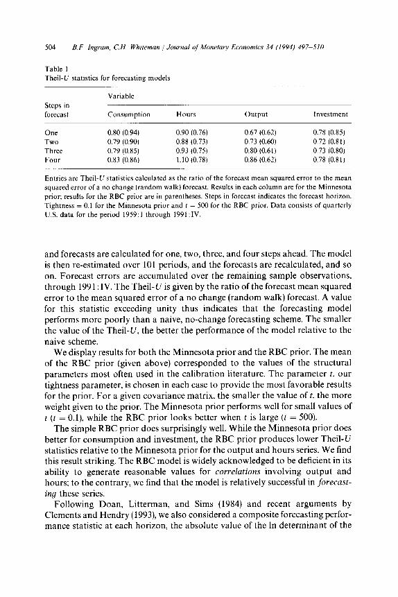
Table 1

The&U statistics for forecasting models

Steps in

forecast

Variable

Consumption Hours output Investment

One 0.80 (0.94) 0.90 (0.76) 0.67 (0.62) 0.78 (0.85) Two 0.79 (0.90) 0.88 (0.73) 0.73 (0.60) 0.72 (0.81) Three 0.79 (0.85) 0.93 (0.75) 0.80 (0.61) 0.73 (0.80) Four 0.83 (0.86) 1.10 (0.78) 0.86 (0.62) 0.78 (0.81)

Entries are Theil-U statistics calculated as the ratio of the forecast mean squared error to the mean

squared error of a no change (random walk) forecast. Results in each column are for the Minnesota

prior; results for the RBC prior are in parentheses. Steps in forecast indicates the forecast horizon.

Tightness = 0.1 for the Minnesota prior and t = 500 for the RBC prior. Data consists of quarterly

U.S. data for the period 1959:1 through 1991 :IV.

and forecasts are calculated for one, two, three, and four steps ahead. The model is then re-estimated over 101 periods, and the forecasts are recalculated, and so on. Forecast errors are accumulated over the remaining sample observations, through 1991: IV. The Theil-U is given by the ratio of the forecast mean squared error to the mean squared error of a no change (random walk) forecast. A value for this statistic exceeding unity thus indicates that the forecasting model performs more poorly than a naive, no-change forecasting scheme, The smaller the value of the Theil-U, the better the performance of the model relative to the naive scheme.

We display results for both the Minnesota prior and the RBC prior. The mean of the RBC prior (given above) corresponded to the values of the structural parameters most often used in the calibration literature. The parameter t, our tightness parameter, is chosen in each case to provide the most favorable results for the prior. For a given covariance matrix, the smaller the value oft, the more weight given to the prior. The Minnesota prior performs well for small values of t (t = O.l), while the RBC prior looks better when t is large (t = 500).

The simple RBC prior does surprisingly well. While the Minnesota prior does better for consumption and investment, the RBC prior produces lower Theil-U statistics relative to the Minnesota prior for the output and hours series. We find this result striking. The RBC model is widely acknowledged to be deficient in its ability to generate reasonable values for correlations involving output and hours; to the contrary, we find that the model is relatively successful in forecast-

ing these series. Following Doan, Litterman, and Sims (1984) and recent arguments by

Clements and Hendry (1993), we also considered a composite forecasting performance statistic at each horizon, the absolute value of the In determinant of the

B.F. Ingram, C.H. Whiteman J Journal ofkfonetar?, Economic.? 34 (1994) 497-5/O 505

Results for Minnesota Pnor

One Step

Two Steps

Three Steps

Four Steps

Results for REK Prior

One Step

Fig. 1. Forecasting performance as a function of prior tightness. The forecast error summary

statistic is calculated as the absolute value of the In determinant of the forecast error covariance

matrix. Steps refers to the forecast horizon.

error covariance matrix of the forecasts. Larger values imply more accurate forecasts. The upper panel in Fig. 1 is a graph of the results derived from using the Minnesota prior and various tightness (c) values. The initial point in this graph, t = 0, corresponds to forecasting each series as if it were a random walk. The Minnesota prior produces better results than the naive random walk specification: the preferred value for t is 0.1. The lower panel in Fig. 1 depicts the results for the RBC prior. Larger values of t improve the forecasting ability of this system. The preferred value here is t = 500. The peak performance of the two priors is nearly indistinguishable. Note that as t increases to infinity, the forecasting performance for each prior will approach the performance of the unrestricted VAR.

More specific information about the statistic is given in Table 2. Here, we compare the forecasting performance of the unrestricted VAR (VAR) to the

506 B.F. Ingram. C.H. Whiteman /Journal qf Monetary Economics 34 (1994) 497-510

Table 2 Multivariate forecasting performance statistics

Model

Unres.

Naive MN

RBC-I

RBC-2

RBC-3

One step Two steps

ABS REL ABS REL

69.71 66.42

70.33 7.79 67.22 9.93 71.14 17.88 68.19 22.13

71.18 18.38 68.20 22.25

71.19 18.50 68.12 21.25

70.75 13.00 67.75 16.63

Three steps

ABS REL

Four steps

ABS REL

65.13 64.24

65.94 10.10 65.58 16.76

66.82 21.13 66.11 23.38

67.03 23.75 66.77 35.13

66.95 22.75 66.15 23.63

66.47 16.75 65.63 17.13

ABS denotes the absolute value of the In determinant of the forecast error covariance matrix: REL

denotes the average percentage improvement in forecast accuracy over the unrestricted model. For

example. the 8.88% improvement of ‘Naive’ over the unrestricted model is calculated as the

difference in In determinants divided by 4 (the number of variables), divided by 2 (to convert

variances to standard errors), multiplied by 100 (to convert to percent). Thus, as noted by Doan,

Litterman. and Sims (1984, p. 20). apart from covariance terms, this quantity comprises the sum of

percentage changes in forecast error standard deviations from each equation. Steps indicate forecast

horizon. Data set consists of quarterly U.S. data for the period 1959:1 through 1991 :IV. ‘Unres.’ denotes an unrestricted VAR. ‘Naive’ a random-walk forecasting model, ‘MN’ a VAR

estimated under a Minnesota prior. and ‘RBC’ a VAR estimated under a RBC prior. Means of the prior distributions for the RBC models are as follows:

Model r B 6 P 1

RBC-1 0.58 0.988 0.025 0.95 200 RBC-2 0.72 0.999 0.0075 0.977 300 RBC-3 0.72 0.999 0.0075 0.96

For the final parameter setting, RBC-3, the t values varied over the four equations. For consump-

tion, t = 120: hours, t = 300; output. t = 175; investment, t = 15.

VAR estimated with the Minnesota prior (MN) and to the naive forecasting scheme (Naive). The naive forecast is derived in a model in which each variable is assumed to follow a univariate random walk (with estimated drift and trend). Real business cycle model results are displayed for three different prior means for p: RBC-1 is the calibrators’ chosen parameter set’ and RBC-2 is the prior mean which yields the best one-step-ahead forecast performance. For RBC-3, we allowed t to vary across the four equations. Underneath each forecast horizon are two columns. The entries in the first column report the absolute value of the In determinant of the forecast error covariance matrix.

bThese values are used by KPR. Hansen (1985) assumes that b = 0.99.

B.F. Ingram. C.H. Whitemnn / Journal of Monetay Economics 34 (1994) 497-510 501

In the second column we have calculated the percentage improvement (or deterioration if negative) of the restricted VAR over the unrestricted VAR. For example, the Minnesota prior improves on the forecasting ability of the unrestricted VAR by 17.88% at the one-step-ahead horizon and 22.13% at the two-step horizon.

Once again, the results for the RBC prior are remarkable. At a one-step-ahead forecast horizon, the usual RBC prior (RBC-1) provides a 18.38% improvement in forecasting performance over an unrestricted VAR. This is comparable to the 17.88% improvement with a Minnesota prior. An exploration of the parameter space returns a parameter vector (RBC-2) which improves the forecasting performance of an unrestricted VAR by 18.5%. The RBC model outperforms the Minnesota prior for this data set over all horizons. We conclude that the RBC model is not only a refinement of the unrestricted model, but also (slightly) of the Minnesota model.

The forecasting results obviously indicate that the RBC model implies relationships among the variables which are closer to those observed in the data than the relationships implied by the Minnesota prior. The Minnesota prior is directed at capturing the persistence in the data variable-by-variable, but neg- lects correlation between the variables. However, there is evidence that the observed data displays cointegrating behavior, which will not be captured by the Minnesota prior. The RBC prior, on the other hand, implies highly persistent series and highly correlated series, as evidenced by the correlation matrices presented above. We conjecture that this feature of the RBC prior is important in forecasting hours and output.

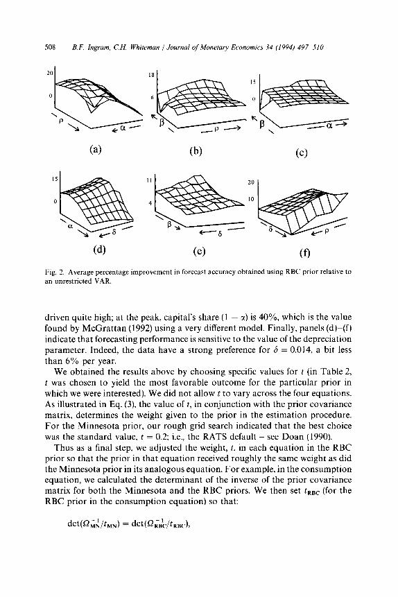
Some information about how the parameters of the prior mean affect forecasting performance is contained in Fig. 2. The panels of the figure record percentage improvement over the unrestricted VAR of mixed RBC-VAR model forecasts for various values of c(, /I, 6, and p in a neighborhood of the best values. Specifically, we conducted a grid search over the hypercube constructed from x E [0.5,0.8], fi E [0.9,1 .O], 6 E [O,O.l], and p E [0.9,1.0]. The three-dimensional graphs depict forecasting performance as a function of two of the hyperparameters given the other two at their ‘peak’ values.

Panel (a) displays a result reminiscent of long-standing estimates of very small capital share parameters (e.g., Bodkin and Klein, 1967): highly persistent technology shocks (high p) together with a low capital share in output (higher Z) do about as well as transient technology shocks together with a high share for capital. Nearly a mirror image of this is found in panel (d), where high depreciation parameters go with low capital shares. Panel (b) suggests that persistence is important in forecasting - either from small discount rates (high /I) or highly persistent technology shocks. Indeed, at low /I, the persistence in the technology shock must be quite large, and p is driven to the boundary value of unity. The peak value corresponds to high values for each of the parameters. Panel (c) indicates a similar tendency: for small /I (below the peak), capital’s share must be

508 B.F. Ingram, C.H. Whiteman 1 Journal of Monetary Economics 34 (1994) 497-510

Fig. 2. Average percentage improvement in forecast accuracy obtained using RBC prior relative to

an unrestricted VAR.

driven quite high; at the peak, capital’s share (1 - c() is 40%, which is the value found by McGrattan (1992) using a very different model. Finally, panels (d)-(f) indicate that forecasting performance is sensitive to the value of the depreciation parameter. Indeed, the data have a strong preference for 6 = 0.014, a bit less than 6% per year.

We obtained the results above by choosing specific values for t (in Table 2, t was chosen to yield the most favorable outcome for the particular prior in which we were interested). We did not allow t to vary across the four equations. As illustrated in Eq. (3), the value of t, in conjunction with the prior covariance matrix, determines the weight given to the prior in the estimation procedure. For the Minnesota prior, our rough grid search indicated that the best choice was the standard value, t = 0.2; i.e., the RATS default - see Doan (1990).

Thus as a final step, we adjusted the weight, t, in each equation in the RBC prior so that the prior in that equation received roughly the same weight as did the Minnesota prior in its analogous equation. For example, in the consumption equation, we calculated the determinant of the inverse of the prior covariance matrix for both the Minnesota and the RBC priors. We then set tRBC (for the RBC prior in the consumption equation) so that:

B.F. Ingram. C.H. Whiteman 1 Journal of Monetary Economics 34 (1994) 497-510 509

where tMN = 0.2. With these values for tRBC, the weight given to the RBC prior is roughly comparable to the weight given to the Minnesota prior. We called this parameter setting RBC-3. Notice that the t values for the RBC prior are much larger than the t values for the Minnesota prior, ranging from 15 to 300. Using these values, the performance of the RBC prior deteriorates. This suggests that our initial comparison did not provide the RBC prior with an unfair advantage relative to the Minnesota prior.

5. Conclusion

The general equilibrium model which we considered in this paper is very basic. That it enables improvements in forecasts of comparable but not superior quality to those produced by the standard random walk specification suggests that other aspects of the structure of real business cycle priors could be exploited to provide still further improvements in forecasting performance. It also hints that more sophisticated dynamic general equilibrium models involving additional economic time series will prove useful in guiding forecasts and policy discussions.

Our results indicate that formal, well-understood Bayesian principles provide a useful foundation for bringing theoretical developments to bear on practical problems of economic forecasting. They also suggest that the approach of viewing the theoretical model as the prior and combining it formally with the information in the data via Bayes’ rule is likely to provide more useful information than the purely theoretical approach (e.g., Hansen and Prescott, 1993) or the purely atheoretical approach (e.g., Sims, 1986): as long as economists agree that theoretical models are false yet provide useful information about the economy, it seems worthwhile to pursue the best of both worlds using formal (Bayesian) procedures specifically developed to do so.

References

Altug. S.. 1989, Time to build and aggregate fluctuations: Some new evidence, International Economic Review 30. 8899920.

Blanchard. 0. and D. Quah, 1989, The dynamic effects of aggregate demand and supply disturbances, American Economic Review 79, 655-673.

Bodkin. R. and L. Klein, 1967. Nonlinear estimation of aggregate production functions, Review of Economics and Statistics 49, 2844.

Braun. R., 1992, Fiscal disturbances and real economic activity in the postwar U.S., Manuscript (Federal Reserve Bank of Minneapolis, Minneapolis, MN).

Clement% M.P. and D.F. Hendry, 1993, On the limitations of comparing mean square forecast errors, Journal of Forecasting 12, 617-637.

Doan, T.. 1990, RATS 3.11 user’s manual (VAR Econometrics. Evanston, IL).

510 B.F. Ingram. C.H. Whiieman / Journal of Monetary Economics 34 (1994) 497-510

Doan, T., R. Litterman. and C. Sims, 1984, Forecasting and conditional projection using realistic prior distributions, Econometric Reviews 3. 1 - 100.

Hansen, G.. 1985, Indivisible labor and the business cycle. Journal of Monetary Economics 19. 1033128.

Hansen. G. and E.C. Prescott. 1993, Did technology shocks cause the 1990-1991 recession?.

American Economic Review Papers and Proceedings 83, 280-286.

Kim. J.Y., 1991. A limited information Bayesian procedure: I. Theoretical investigation, Manuscript (Yale University, New Haven, CT).

King, R.G., C.I. Plosser. and ST. Rebelo, 1988, Production, growth. and business cycles: 1. The basic neoclassical model, Journal of Monetary Economics 21. 195-232.

Kwan, Y.K., 1990a. Bayesian model calibration. with an application to a non-linear rational

expectation two-country model, Manuscript (University of Chicago, Graduate School of Busi- ness, Chicago, IL).

Kwan. Y.K., 1990b. Bayesian analysis with an unknown likelihood function A limited information

approach, Manuscript (University of Chicago, Graduate School of Business, Chicago. IL).

Kydland, F. and E. Prescott. 1982, Time to build and aggregate fluctuations. Econometrica 50. 1345-1370.

Leeper, E. and D. Gordon. 1992, In search of the liquidity effect, Journal of Monetary Economics 29, 341-369.

Litterman. R.B., 1984, Specifying vector autoregressions for macroeconomic forecasting, in: P. Goel.

ed.. Bayesian inference and decision techniques with applications: Essays in honor of Bruno de

Finetti (North-Holland, Amsterdam).

McGrattan, E.. 1992. The macroeconomic effects of distortionary taxation, Manuscript (Federal

Reserve Bank of Minneapolis. Minneapolis, MN).

Sims, C.. 1980. Macroeconomics and reality, Econometrica 48, l-48. Sims, C.. 1986, Are forecasting models usable for policy analysis?, Federal Reserve Bank of

Minneapolis Quarterly Review 10. 2216.

Theil, H., 1971, Principles of econometrics (Wiley. New York, NY).

Supplanting the ‘Minnesota’ prior Forecasting...

Documents

Transcript of Supplanting the ‘Minnesota’ prior Forecasting...