Stochastic Optimization and Variational Inference · Stochastic Optimization and Variational...
58
Stochastic Optimization and Variational Inference David M. Blei Columbia University November 23, 2014
Transcript of Stochastic Optimization and Variational Inference · Stochastic Optimization and Variational...

Stochastic Optimization and Variational Inference
David M. Blei
Columbia University
November 23, 2014

Communities discovered in a 3.7M node network of U.S. Patents
[Gopalan and Blei, PNAS 2013]

Hoffman, Blei, Wang, and Paisley
game
second
seasonteam
play
games
players
points
coach
giants
streetschool
house
life
children
familysays
night
man
know
life
says
show
mandirector
television
film
story
movie
films
house
life
children
man
war
book
story
books
author
novel
street
house
nightplace
park
room
hotel
restaurant
garden
wine
house
bush
political
party
clintoncampaign
republican
democratic
senatordemocrats percent
street
house
building
real
spacedevelopment
squarehousing
buildings
game
secondteam
play
won
open
race
win
roundcup
game
season
team
runleague
gameshit
baseball
yankees
mets
government
officials
warmilitary
iraq
army
forces
troops
iraqi
soldiers
school
life
children
family
says
women
helpmother
parentschild
percent
business
market
companies
stock
bank
financial
fund
investorsfunds government
life
warwomen
politicalblack
church
jewish
catholic
pope
street
show
artmuseum
worksartists
artist
gallery
exhibitionpaintings street
yesterdaypolice
man
casefound
officer
shot
officers
charged
1 2 3 4 5
6 7 8 9 10
11 12 13 14 15
Figure 10: The 15 most frequent topics from the HDP posterior on the New YorkTimes. Each topic plot illustrates the topic’s most frequent words.
42
Topics found in 1.8M articles from the New York Times
[Hoffman, Blei, Wang, Paisley, JMLR 2013]

Adygei BalochiBantuKenyaBantuSouthAfricaBasque Bedouin BiakaPygmy Brahui BurushoCambodianColombianDai Daur Druze French Han Han−NChinaHazaraHezhenItalian Japanese Kalash KaritianaLahu Makrani Mandenka MayaMbutiPygmyMelanesianMiaoMongola Mozabite NaxiOrcadianOroqen Palestinian Papuan Pathan Pima Russian San Sardinian She Sindhi Surui Tu TujiaTuscanUygurXibo Yakut Yi Yoruba
prob
pops1234567
Population analysis of 2 billion genetic measurements
[Gopalan, Hao, Blei, Storey, in preparation]

Neuroscience analysis of 220 million fMRI measurements
[Manning et al., PLOS ONE 2014]

The probabilistic pipeline
Build model Infer hidden variables
Data
Predict & Explore
I Customized data analysis is important to many fields.
I Pipeline separates assumptions, computation, application
I Eases collaborative solutions to data science problems

The probabilistic pipeline
Build model Infer hidden variables
Data
Predict & Explore
I Inference is the key algorithmic problem.
I Answers the question: What does this model say about this data?
I Our goal: General and scalable approaches to inference

The probabilistic pipeline
Build model Infer hidden variables
Data
Predict & Explore
I Variational methods turn inference into optimization.
I With stochastic optimization:
– Scale up with stochastic variational inference [Hoffman et al., 2013]
– Generalize with black box variational inference [Ranganath et al., 2014]

Stochastic Variational Inference(with Matt Hoffman, Chong Wang, John Paisley)

Example: Latent Dirichlet allocation (LDA)
gene 0.04dna 0.02genetic 0.01.,,
life 0.02evolve 0.01organism 0.01.,,
brain 0.04neuron 0.02nerve 0.01...
data 0.02number 0.02computer 0.01.,,
Topics Documents Topic proportions andassignments
I Each topic is a distribution over words
I Each document is a mixture of corpus-wide topics
I Each word is drawn from one of those topics

Example: Latent Dirichlet allocation (LDA)
Topics Documents Topic proportions andassignments
I But we only observe the documents; the other structure is hidden.
I We compute the posterior
p.topics, proportions, assignments j documents/

Example inference
1 8 16 26 36 46 56 66 76 86 96
Topics
Probability
0.0
0.1
0.2
0.3
0.4

Example inference
“Genetics” “Evolution” “Disease” “Computers”
human evolution disease computergenome evolutionary host models
dna species bacteria informationgenetic organisms diseases datagenes life resistance computers
sequence origin bacterial systemgene biology new network
molecular groups strains systemssequencing phylogenetic control model
map living infectious parallelinformation diversity malaria methods
genetics group parasite networksmapping new parasites softwareproject two united new
sequences common tuberculosis simulations

LDA as a graphical model
Proportionsparameter
Per-documenttopic proportions
Per-wordtopic assignment
Observedword Topics
Topicparameter
˛ ✓d zd;n wd;n ˇkN D
⌘
K
I Encodes assumptions about data with a factorization of the joint
I Connects assumptions to algorithms for computing with data
I Defines the posterior (through the joint)

Posterior inference
˛ ✓d zd;n wd;n ˇkN D
⌘
K
I The posterior of the latent variables given the documents is
p.ˇ; �; z jw/ D p.ˇ; �; z; w/Rˇ
R�
Pz p.ˇ; �; z; w/
:
I We can’t compute the denominator, the marginal p.w/.
I As for many interesting models, we use approximate inference.
Classical variational inference
˛ ✓d zd;n wd;n ˇkN D
⌘
K
I Given data, estimate the conditional distribution of the hidden variables.
– Local variables describe per-data point hidden structure.– Global variables describe structure shared by all the data.
I Classical variational inference is inefficient:
– Do some local computation for each data point.– Aggregate these computations to re-estimate global structure.– Repeat.

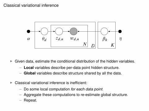
Stochastic variational inference
Adygei BalochiBantuKenyaBantuSouthAfricaBasque Bedouin BiakaPygmy Brahui BurushoCambodianColombianDai Daur Druze French Han Han−NChinaHazaraHezhenItalian Japanese Kalash KaritianaLahu Makrani Mandenka MayaMbutiPygmyMelanesianMiaoMongola Mozabite NaxiOrcadianOroqen Palestinian Papuan Pathan Pima Russian San Sardinian She Sindhi Surui Tu TujiaTuscanUygurXibo Yakut Yi Yoruba
prob
pops1234567
GLOBAL HIDDEN STRUCTURE
SUBSAMPLE DATA
INFER LOCAL
STRUCTURE
UPDATE GLOBAL
STRUCTURE
MASSIVEDATA SET

Stochastic variational inference
4096
systemshealth
communicationservicebillion
languagecareroad
8192
servicesystemshealth
companiesmarket
communicationcompanybillion
12288
servicesystemscompaniesbusinesscompanybillionhealthindustry
16384
servicecompaniessystemsbusinesscompanyindustrymarketbillion
32768
businessservice
companiesindustrycompany
managementsystemsservices
49152
businessservice
companiesindustryservicescompany
managementpublic
2048
systemsroadmadeservice
announcednationalwest
language
65536
businessindustryservice
companiesservicescompany
managementpublic
Documentsanalyzed
Top eightwords
Documents seen (log scale)
Perplexity
600
650
700
750
800
850
900
103.5
104
104.5
105
105.5
106
106.5
Batch 98K
Online 98K
Online 3.3M
[Hoffman et al., 2010]

Hoffman, Blei, Wang, and Paisley
game
second
seasonteam
play
games
players
points
coach
giants
streetschool
house
life
children
familysays
night
man
know
life
says
show
mandirector
television
film
story
movie
films
house
life
children
man
war
book
story
books
author
novel
street
house
nightplace
park
room
hotel
restaurant
garden
wine
house
bush
political
party
clintoncampaign
republican
democratic
senatordemocrats percent
street
house
building
real
spacedevelopment
squarehousing
buildings
game
secondteam
play
won
open
race
win
roundcup
game
season
team
runleague
gameshit
baseball
yankees
mets
government
officials
warmilitary
iraq
army
forces
troops
iraqi
soldiers
school
life
children
family
says
women
helpmother
parentschild
percent
business
market
companies
stock
bank
financial
fund
investorsfunds government
life
warwomen
politicalblack
church
jewish
catholic
pope
street
show
artmuseum
worksartists
artist
gallery
exhibitionpaintings street
yesterdaypolice
man
casefound
officer
shot
officers
charged
1 2 3 4 5
6 7 8 9 10
11 12 13 14 15
Figure 10: The 15 most frequent topics from the HDP posterior on the New YorkTimes. Each topic plot illustrates the topic’s most frequent words.
42
Topics found in 1.8M articles from the New York Times

Stochastic variational inference
SUBSAMPLE DATA
INFER LOCAL
STRUCTURE
UPDATE GLOBAL
STRUCTURE
1. Define a generic class of models
2. Derive classical mean-field variational inference
3. Use the classical algorithm to derive stochastic variational inference

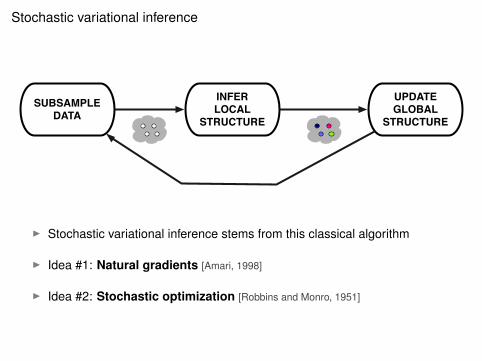
A generic class of models
Global variables
Local variables
ˇ
xizin
p.ˇ; z1Wn; x1Wn/ D p.ˇ/nYiD1
p.zi jˇ/p.xi j zi ; ˇ/
A generic model with local and global variables:
I The observations are x D x1Wn.
I The local variables are z D z1Wn.
I The global variables are ˇ.
I The i th data point xi only depends on zi and ˇ.
Our goal is to compute p.ˇ; z j x/.

A generic class of models
Global variables
Local variables
ˇ
xizin
p.ˇ; z1Wn; x1Wn/ D p.ˇ/nYiD1
p.zi jˇ/p.xi j zi ; ˇ/
I A complete conditional is the conditional of a latent variable given theobservations and other latent variable.
I Assume each complete conditional is in the exponential family,
p.zi jˇ; xi / D h.zi / expf�`.ˇ; xi />zi � a.�`.ˇ; xi //gp.ˇ j z; x/ D h.ˇ/ expf�g.z; x/>ˇ � a.�g.z; x//g:

A generic class of models
Global variables
Local variables
ˇ
xizin
p.ˇ; z1Wn; x1Wn/ D p.ˇ/nYiD1
p.zi jˇ/p.xi j zi ; ˇ/
I Bayesian mixture models
I Time series models(variants of HMMs, Kalman filters)
I Factorial models
I Matrix factorization(e.g., factor analysis, PCA, CCA)
I Dirichlet process mixtures, HDPs
I Multilevel regression(linear, probit, Poisson)
I Stochastic blockmodels
I Mixed-membership models(LDA and some variants)

Mean-field variational inference
ELBO
ˇ
xi
n
zi
nzi
ˇ�
�i
I Introduce a variational distribution over the latent variables q.ˇ; z/.
I Optimize the evidence lower bound (ELBO) with respect to q,
logp.x/ � EqŒlogp.ˇ;Z; x/� � EqŒlog q.ˇ;Z/�:
I Equivalent to minimizing the KL between q and the posterior
I The ELBO links the observations/model to the variational distribution.

Mean-field variational inference
ELBO
ˇ
xi
n
zi
nzi
ˇ�
�i
I Set q.ˇ; z/ to be a fully factored variational distribution,
q.ˇ; z/ D q.ˇ j�/QniD1 q.zi j�i /:
I Recall the complete conditional is in the exponential family
p.ˇ j z; x/ D h.ˇ/ expf�g.z; x/>ˇ � a.�g.z; x//gI Set each factor to be in the same family
q.ˇ j�/ D h.ˇ/ expf�>ˇ � a.�/g:

Mean-field variational inference
ELBO
ˇ
xi
n
zi
nzi
ˇ�
�i
I We will optimize the ELBO with coordinate ascent.
I The gradient with respect to the global variational parameters is
r�L D a00.�/.E� Œ�g.Z; x/� � �/:I This leads to a simple coordinate update [Ghahramani and Beal, 2001]
�� D E���g.Z; x/
�:

Mean-field variational inference for LDA
�ˇkwd;nzd;n�d˛N D K
�d �d;n �k
I Local: Per-document topic proportions � and topic assignments z1WN .
I Global: Topics ˇ1WKI The variational distribution is
q.ˇ; �; z/ DKYkD1
q.ˇk j�k/DYdD1
q.�d j d /NYnD1
q.zd;n j�d;n/

Mean-field variational inference for LDA
�ˇkwd;nzd;n�d˛N D K
�d �d;n �k
I Local:Fix the topics. Iteratively update the parameters for each document.
.tC1/ D ˛ CPNnD1 �
.t/n
�.tC1/n / expfEqŒlog ��C EqŒlogˇ:;wn�g

Mean-field variational inference for LDA
1 8 16 26 36 46 56 66 76 86 96
Topics
Probability
0.0
0.1
0.2
0.3
0.4

Mean-field variational inference for LDA
�ˇkwd;nzd;n�d˛N D K
�d �d;n �k
I Global:Aggregate the local computations. Update the parameters for the topics.
�k D �CXd
Xn
wd;n�d;n

Mean-field variational inference for LDA
“Genetics” “Evolution” “Disease” “Computers”
human evolution disease computergenome evolutionary host models
dna species bacteria informationgenetic organisms diseases datagenes life resistance computers
sequence origin bacterial systemgene biology new network
molecular groups strains systemssequencing phylogenetic control model
map living infectious parallelinformation diversity malaria methods
genetics group parasite networksmapping new parasites softwareproject two united new
sequences common tuberculosis simulations

Mean-field variational inference
Initialize � randomly.Repeat until the ELBO converges
1. For each data point, update the local variational parameters:
�.t/i D E�.t�1/ Œ�`.ˇ; xi /� for i 2 f1; : : : ; ng:
2. Update the global variational parameters:
�.t/ D E�.t/ Œ�g.Z1Wn; x1Wn/�:
I Inefficient: We analyze the whole data set before completing one iteration.
I E.g.: In iteration #1 we analyze all documents with random topics.
Stochastic variational inference
SUBSAMPLE DATA
INFER LOCAL
STRUCTURE
UPDATE GLOBAL
STRUCTURE
I Stochastic variational inference stems from this classical algorithm
I Idea #1: Natural gradients [Amari, 1998]
I Idea #2: Stochastic optimization [Robbins and Monro, 1951]

Natural gradients RIEMANNIAN CONJUGATE GRADIENT FOR VB
!"#$%&'()*+'(,%))'%)-#$%&'()*
Figure 1: Gradient and Riemannian gradient directions are shown for the mean of distribution q.VB learning with a diagonal covariance is applied to the posterior p(x,y) ! exp[!9(xy!1)2! x2! y2]. The Riemannian gradient strengthens the updates in the directions wherethe uncertainty is large.
the conjugate gradient algorithm with their Riemannian counterparts: Riemannian inner productsand norms, parallel transport of gradient vectors between different tangent spaces as well as linesearches and steps along geodesics in the Riemannian space. In practical algorithms some of thesecan be approximated by their flat-space counterparts. We shall apply the approximate Riemannianconjugate gradient (RCG) method which implements Riemannian (natural) gradients, inner productsand norms but uses flat-space approximations of the others as our optimisation algorithm of choicethroughout the paper. As shown in Appendix A, these approximations do not affect the asymptoticconvergence properties of the algorithm. The difference between gradient and conjugate gradientmethods is illustrated in Figure 2.
In this paper we propose using the Riemannian structure of the distributions q("""|###) to derivemore efficient algorithms for approximate inference and especially VB using approximations witha fixed functional form. This differs from the traditional natural gradient learning by Amari (1998)which uses the Riemannian structure of the predictive distribution p(XXX |"""). The proposed methodcan be used to jointly optimise all the parameters ### of the approximation q("""|###), or in conjunctionwith VB EM for some parameters.
3239
[Honkela et al., 2010]
I The natural gradient of the ELBO [Sato, 2001]
Or�L D E� Œ�g.Z; x/� � �:I Computationally:
– Compute coordinate updates in parallel.– Subtract the current variational parameters.

Stochastic optimization
Institute of Mathematical Statistics is collaborating with JSTOR to digitize, preserve, and extend access toThe Annals of Mathematical Statistics.
www.jstor.org®
I Replace the gradient with cheaper noisy estimates [Robbins and Monro, 1951]
I Guaranteed to converge to a local optimum [Bottou, 1996]
I Has enabled modern machine learning

Stochastic variational inference
ELBO
ˇ
xi
n
zi
nzi
ˇ�
�i
I We will use stochastic optimization for global variables.
I Let r�Lt be a realization of a random variable whose expectation is r�L.
I Iteratively set�.t/ D �.t�1/ C �tr�Lt
I This leads to a local optimum when1XtD1
�t D11XtD1
�2t <1

Stochastic variational inference
I Decompose the ELBO
L D EŒlogp.ˇ/��EŒlog q.ˇ/�CPniD1 EŒlogp.zi ; xi jˇ/��EŒlog q.zi /�
I Uniformly sample a single data point xt . Define
Lt , EŒlogp.ˇ/��EŒlog q.ˇ/�Cn.EŒlogp.zt ; xt jˇ/��EŒlog q.zt /�/:
1. The t -ELBO Lt is a noisy estimate of the ELBO, Et ŒLt � D L.2. The gradient of Lt is a noisy gradient of the ELBO.3. The t -ELBO is an ELBO where we saw xt repeatedly.
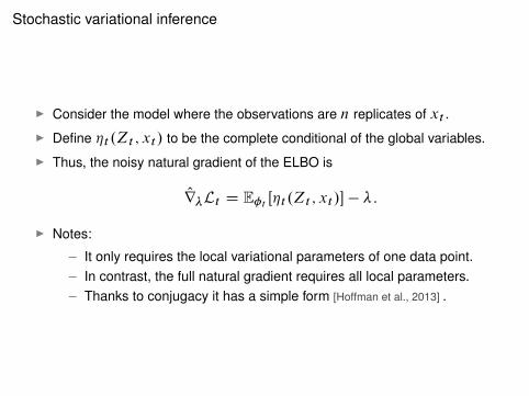
Stochastic variational inference
I Consider the model where the observations are n replicates of xt .
I Define �t .Zt ; xt / to be the complete conditional of the global variables.
I Thus, the noisy natural gradient of the ELBO is
Or�Lt D E�tŒ�t .Zt ; xt /� � �:
I Notes:
– It only requires the local variational parameters of one data point.– In contrast, the full natural gradient requires all local parameters.– Thanks to conjugacy it has a simple form [Hoffman et al., 2013] .

Stochastic variational inference
Initialize global parameters � randomly.Set the step-size schedule �t appropriately.Repeat forever
1. Sample a data point uniformly,
xt � Uniform.x1; : : : ; xn/:
2. Compute its local variational parameter,
� D E�.t�1/ Œ�`.ˇ; xt /�:
3. Pretend its the only data point in the data set,
O� D E� Œ�t .Zt ; xt /�:
4. Update the current global variational parameter,
�.t/ D .1 � �t /�.t�1/ C �t O�:

Stochastic variational inference in LDA
˛ ✓d zd;n wd;n ˇkN D
⌘
K
1. Sample a document.
2. Estimate the local variational parameters using the current topics.
3. Form intermediate topics from those local parameters.
4. Update topics as a weighted average of intermediate and current topics.

Stochastic variational inference in LDA
4096
systemshealth
communicationservicebillion
languagecareroad
8192
servicesystemshealth
companiesmarket
communicationcompanybillion
12288
servicesystemscompaniesbusinesscompanybillionhealthindustry
16384
servicecompaniessystemsbusinesscompanyindustrymarketbillion
32768
businessservice
companiesindustrycompany
managementsystemsservices
49152
businessservice
companiesindustryservicescompany
managementpublic
2048
systemsroadmadeservice
announcednationalwest
language
65536
businessindustryservice
companiesservicescompany
managementpublic
Documentsanalyzed
Top eightwords
Documents seen (log scale)
Perplexity
600
650
700
750
800
850
900
103.5
104
104.5
105
105.5
106
106.5
Batch 98K
Online 98K
Online 3.3M
[Hoffman et al., 2010]

Stochastic variational inference
SUBSAMPLE DATA
INFER LOCAL
STRUCTURE
UPDATE GLOBAL
STRUCTURE
We derived an algorithm for scalable variational inference.
I Bayesian mixture models
I Time series models(variants of HMMs, Kalman filters)
I Factorial models
I Matrix factorization(e.g., factor analysis, PCA, CCA)
I Dirichlet process mixtures, HDPs
I Multilevel regression(linear, probit, Poisson)
I Stochastic blockmodels
I Mixed-membership models(LDA and some variants)

Black Box Variational Inference(with Rajesh Ranganath and Sean Gerrish)

Black box variational inference
Build model Infer hidden variables
Data
Predict & Explore
I Approximate inference can be difficult to derive.
I Especially true for models that are not conditionally conjugate.(Discrete choice models, Bayesian generalized linear models, ...)
I Keeps us from trying many models.

REUSABLE VARIATIONAL
FAMILIESBLACK BOX
VARIATIONAL INFERENCE
MASSIVE DATA SET
p.z j x/
ANY MODEL
REUSABLE VARIATIONAL
FAMILIES
REUSABLE VARIATIONAL
FAMILIES
I Easily use variational inference with any modelI No requirements on the complete conditionalsI No mathematical work beyond specifying the model

Black box variational inference
ELBO
ˇ
xi
n
zi
nzi
ˇ�
�i
The idea:
I Avoid computing model specific expectations and gradients.
I Construct noisy gradients by sampling from the variational distribution.
I Use stochastic optimization to maximize the ELBO

Black box variational inference
ELBO
ˇ
xi
n
zi
nzi
ˇ�
�i
The ELBO:L.�/ D EqŒlogp.ˇ;Z; x/� � log q�.ˇ;Z/�
Its gradient:
r�L.�/ D EqŒr� log q�.ˇ;Z/.logp.ˇ;Z; x/ � log q�.ˇ;Z//�

Black box variational inference
ELBO
ˇ
xi
n
zi
nzi
ˇ�
�i
A noisy gradient at �:
r�L.�/ � 1
B
BXbD1
.r� log q�.ˇb; zb// .logp.ˇb; zb; x/ � log q�.ˇb; zb//
where.ˇb; zb/ � q�.ˇ; z/

The noisy gradient
r�L.�/ � 1
B
BXbD1
.r� log q�.ˇb; zb//.logp.ˇb; zb; x/� log q�.ˇb; zb//
I We use these gradients in a stochastic optimization algorithm.
I Requirements:
– Sampling from q�.ˇ; z/
– Evaluating r� log q�.ˇ; z/– Evaluating logp.ˇ; z; x/
I A black box: q.�/ can be reused across models;

The noisy gradient
r�L.�/ � 1
B
BXbD1
.r� log q�.ˇb; zb//.logp.ˇb; zb; x/� log q�.ˇb; zb//
Extensions:
I Rao-Blackwellization for each component of the gradient
I Control variates, again using r� log q�.ˇ; z/I AdaGrad, for setting learning rates [Duchi, Hazan, Singer, 2011]
I Stochastic variational inference, for handling massive data

−150
−100
−50
0
0 5 10 15 20time
pred
ictiv
e lik
elih
ood
name
gibbs
vi
BBVI versus MH-in-Gibbs(on a Nonconjugate Normal-Gamma time-series model)

Neuroscience analysis of 220 million fMRI measurements
[Manning et al., PLOS ONE 2014]
zn;`;kw`,k
w`+1,k zn;`C1;k
K`
KL
zn;L;k⌘
K1
zn;1;kw1,k
xn;iw0,i
V
������
N
K`C1
��!�)&))��!��#�����) ))��!��#�����)�))����)%���'
������!�� )&))) �����$� �)!��!�)))����)�"� �)))������#�����"��������) ����� �'
�����)&))����)� � �))���)��)��)�� �)&))))�"���)()������������))'))���)��)��)����)&))))���)��)��)�� �)&))))))� ���)�)����!��!�����)))))))))))))))�)�����������%�����"���� ��������))))'))����)�)����)�)���� "���$��� �))''
Initial state 1st iteration 5th (and last) iteration
Figure 2. The approximate predictive distribution given by variational inference at different stages of the algorithm. Thedata are 100 points generated by a Gaussian DP mixture model with fixed diagonal covariance.
5 10 20 30 40 50
050
010
0015
0020
00
Dimension
Tim
e (s
econ
ds)
VarTDPCDP
5 10 20 30 40 50
−120
0−8
00−4
00
Dimension
Hel
d−ou
t log
like
lihoo
d
Figure 3. (Left) Convergence time per dimension across ten datasets for variational inference (Var), the TDP Gibbssampler (TDP), and the collapsed Gibbs sampler (CDP). Grey bars are standard error. (Right) Average held-out loglikelihood for the corresponding predictive distributions.
The update for the variational multinomial on Zn isφn,i ∝ exp(E) where:
E = E [log Vi | γi] + E [ηi | τi]T
Xn
− E [a(ηi) | τi] +!i−1
j=1 E [log(1 − Vj) | γj ] .
Iterating between these updates is a coordinate ascentalgorithm for optimizing Eq. (12) with respect to theparameters in Eq. (13). We thus find q(v,η∗, z) whichis closest, within the confines of its parameters, to thetrue posterior. This yields an approximate predictivedistribution of the next data point given, as in theTDP Gibbs sampler for a single sample, by Eq. (10).
5. Example and Results
We applied the variational algorithm of Section 4 andthe two Gibbs samplers of Section 3 to Gaussian-
Gaussian DP mixture models. The data are assumeddrawn from a multivariate Gaussian with fixed covari-ance matrix; the mean of each data point is drawnfrom a DP with a Gaussian baseline distribution (i.e.,the conjugate prior).
In Figure 2, we illustrate the variational inference algo-rithm on a toy problem. We have simulated 100 datapoints from a two-dimensional Gaussian-Gaussian DPmixture with diagonal covariance. We illustrate thedata and the predictive distribution given by the varia-tional inference algorithm of Section 4 with variationaltruncation level K equal to 20. In the initial setting,the variational approximation places a largely flat dis-tribution on the data. After one iteration, the algo-rithm has found the various modes of the data and,after convergence, it has further refined those modes.Notice that even though we represent 20 mixture com-
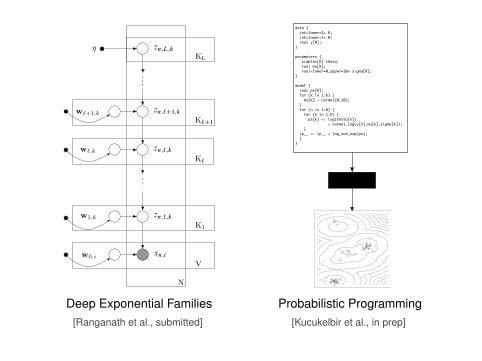
Deep Exponential Families Probabilistic Programming[Ranganath et al., submitted] [Kucukelbir et al., in prep]

The probabilistic pipeline
Build model Infer hidden variables
Data
Predict & Explore
I Customized data analysis is important to many fields.
I Pipeline separates assumptions, computation, application
I Eases collaborative solutions to data science problems

The probabilistic pipeline
Build model Infer hidden variables
Data
Predict & Explore
I Inference is the key algorithmic problem.
I Answers the question: What does this model say about this data?
I Our goal: General and scalable approaches to inference

Adygei BalochiBantuKenyaBantuSouthAfricaBasque Bedouin BiakaPygmy Brahui BurushoCambodianColombianDai Daur Druze French Han Han−NChinaHazaraHezhenItalian Japanese Kalash KaritianaLahu Makrani Mandenka MayaMbutiPygmyMelanesianMiaoMongola Mozabite NaxiOrcadianOroqen Palestinian Papuan Pathan Pima Russian San Sardinian She Sindhi Surui Tu TujiaTuscanUygurXibo Yakut Yi Yoruba
prob
pops1234567
GLOBAL HIDDEN STRUCTURE
SUBSAMPLE DATA
INFER LOCAL
STRUCTURE
UPDATE GLOBAL
STRUCTURE
MASSIVEDATA SET
“Stochastic variational inference” [Hoffman et al., 2013, JMLR]

REUSABLE VARIATIONAL
FAMILIESBLACK BOX
VARIATIONAL INFERENCE
MASSIVE DATA SET
p.z j x/
ANY MODEL
REUSABLE VARIATIONAL
FAMILIES
REUSABLE VARIATIONAL
FAMILIES
“Black box variational inference [Ranganath et al., 2013, AISTATS]

Build model Infer hidden variables
Data
Predict & Explore
Criticize model
Revise