Fast Second-Order Stochastic Backpropagation forVariational Inference

Kai FanDuke University

kai.fan@stat.duke.edu

Ziteng Wang∗HKUST†

wangzt2012@gmail.com

Jeffrey BeckDuke University

jeff.beck@duke.edu

James T. KwokHKUST

jamesk@cse.ust.hk

Katherine HellerDuke University

kheller@gmail.com

Abstract

We propose a second-order (Hessian or Hessian-free) based optimization methodfor variational inference inspired by Gaussian backpropagation, and argue thatquasi-Newton optimization can be developed as well. This is accomplished bygeneralizing the gradient computation in stochastic backpropagation via a repa-rameterization trick with lower complexity. As an illustrative example, we ap-ply this approach to the problems of Bayesian logistic regression and variationalauto-encoder (VAE). Additionally, we compute bounds on the estimator varianceof intractable expectations for the family of Lipschitz continuous function. Ourmethod is practical, scalable and model free. We demonstrate our method on sev-eral real-world datasets and provide comparisons with other stochastic gradientmethods to show substantial enhancement in convergence rates.

1 Introduction

Generative models have become ubiquitous in machine learning and statistics and are now widelyused in fields such as bioinformatics, computer vision, or natural language processing. These modelsbenefit from being highly interpretable and easily extended. Unfortunately, inference and learningwith generative models is often intractable, especially for models that employ continuous latentvariables, and so fast approximate methods are needed. Variational Bayesian (VB) methods [1] dealwith this problem by approximating the true posterior that has a tractable parametric form and thenidentifying the set of parameters that maximize a variational lower bound on the marginal likelihood.That is, VB methods turn an inference problem into an optimization problem that can be solved, forexample, by gradient ascent.

Indeed, efficient stochastic gradient variational Bayesian (SGVB) estimators have been devel-oped for auto-encoder models [17] and a number of papers have followed up on this approach[28, 25, 19, 16, 15, 26, 10]. Recently, [25] provided a complementary perspective by using stochasticbackpropagation that is equivalent to SGVB and applied it to deep latent gaussian models. Stochas-tic backpropagation overcomes many limitations of traditional inference methods such as the mean-field or wake-sleep algorithms [12] due to the existence of efficient computations of an unbiasedestimate of the gradient of the variational lower bound. The resulting gradients can be used for pa-rameter estimation via stochastic optimization methods such as stochastic gradient decent(SGD) oradaptive version (Adagrad) [6].

∗Equal contribution as the first author†Refer to Hong Kong University of Science and Technology

1

arX

iv:1

509.

0286

6v2

[st

at.M

L]

28

Mar

201

7

Unfortunately, methods such as SGD or Adagrad converge slowly for some difficult-to-train models,such as untied-weights auto-encoders or recurrent neural networks. The common experience is thatgradient decent always gets stuck near saddle points or local extrema. Meanwhile the learning rateis difficult to tune. [18] gave a clear explanation on why Newton’s method is preferred over gradientdecent, which often encounters under-fitting problem if the optimizing function manifests patholog-ical curvature. Newton’s method is invariant to affine transformations so it can take advantage ofcurvature information, but has higher computational cost due to its reliance on the inverse of theHessian matrix. This issue was partially addressed in [18] where the authors introduced Hessianfree (HF) optimization and demonstrated its suitability for problems in machine learning.

In this paper, we continue this line of research into 2nd order variational inference algorithms. In-spired by the property of location scale families [8], we show how to reduce the computationalcost of the Hessian or Hessian-vector product, thus allowing for a 2nd order stochastic optimiza-tion scheme for variational inference under Gaussian approximation. In conjunction with the HFoptimization, we propose an efficient and scalable 2nd order stochastic Gaussian backpropagationfor variational inference called HFSGVI. Alternately, L-BFGS [3] version, a quasi-Newton methodmerely using the gradient information, is a natural generalization of 1st order variational inference.

The most immediate application would be to look at obtaining better optimization algorithms forvariational inference. As to our knowledge, the model currently applying 2nd order information isLDA [2, 14], where the Hessian is easy to compute [11]. In general, for non-linear factor modelslike non-linear factor analysis or the deep latent Gaussian models this is not the case. Indeed,to our knowledge, there has not been any systematic investigation into the properties of variousoptimization algorithms and how they might impact the solutions to optimization problem arisingfrom variational approximations.

The main contributions of this paper are to fill such gap for variational inference by introducing anovel 2nd order optimization scheme. First, we describe a clever approach to obtain curvature infor-mation with low computational cost, thus making the Newton’s method both scalable and efficient.Second, we show that the variance of the lower bound estimator can be bounded by a dimension-freeconstant, extending the work of [25] that discussed a specific bound for univariate function. Third,we demonstrate the performance of our method for Bayesian logistic regression and the VAE modelin comparison to commonly used algorithms. Convergence rate is shown to be competitive or faster.

2 Stochastic Backpropagation

In this section, we extend the Bonnet and Price theorem [4, 24] to develop 2nd order Gaussianbackpropagation. Specifically, we consider how to optimize an expectation of the form Eqθ [f(z|x)],where z and x refer to latent variables and observed variables respectively, and expectation is takenw.r.t distribution qθ and f is some smooth loss function (e.g. it can be derived from a standardvariational lower bound [1]). Sometimes we abuse notation and refer to f(z) by omitting x when noambiguity exists. To optimize such expectation, gradient decent methods require the 1st derivatives,while Newton’s methods require both the gradients and Hessian involving 2nd order derivatives.

2.1 Second Order Gaussian Backpropagation

If the distribution q is a dz-dimensional GaussianN (z|µ,C), the required partial derivative is easilycomputed with a lower algorithmic costO(d2z) [25]. By using the property of Gaussian distribution,we can compute the 2nd order partial derivative of EN (z|µ,C)[f(z)] as follows:

∇2µi,µjEN (z|µ,C)[f(z)] = EN (z|µ,C)[∇2

zi,zjf(z)] = 2∇CijEN (z|µ,C)[f(z)], (1)

∇2Ci,j ,Ck,l

EN (z|µ,C)[f(z)] =1

4EN (z|µ,C)[∇4

zi,zj ,zk,zlf(z)], (2)

∇2µi,Ck,l

EN (z|µ,C)[f(z)] =1

2EN (z|µ,C)

[∇3zi,zk,zl

f(z)]. (3)

Eq. (1), (2), (3) (proof in supplementary) have the nice property that a limited number of samplesfrom q are sufficient to obtain unbiased gradient estimates. However, note that Eq. (2), (3) needsto calculate the third and fourth derivatives of f(z), which is highly computationally inefficient. Toavoid the calculation of high order derivatives, we use a co-ordinate transformation.

2

2.2 Covariance Parameterization for Optimization

By constructing the linear transformation (a.k.a. reparameterization) z = µ + Rε, where ε ∼N (0, Idz ), we can generate samples from any Gaussian distribution N (µ,C) by simulating datafrom a standard normal distribution, provided the decomposition C = RR> holds. This fact allowsus to derive the following theorem indicating that the computation of 2nd order derivatives can bescalable and programmed to run in parallel.

Theorem 1 (Fast Derivative). If f is a twice differentiable function and z follows Gaussian dis-tribution N (µ,C), C = RR>, where both the mean µ and R depend on a d-dimensional pa-rameter θ = (θl)

dl=1, i.e. µ(θ),R(θ), we have ∇2

µ,REN (µ,C)[f(z)] = Eε∼N (0,Idz )[ε> ⊗H], and

∇2REN (µ,C)[f(z)] = Eε∼N (0,Idz )

[(εεT )⊗H]. This then implies

∇θlEN (µ,C)[f(z)] = Eε∼N (0,I)

[g>

∂(µ+ Rε)

∂θl

], (4)

∇2θl1θl2

EN (µ,C)[f(z)] = Eε∼N (0,I)

[∂(µ+ Rε)

∂θl1

>H∂(µ+ Rε)

∂θl2+ g>

∂2(µ+ Rε)

∂θl1∂l2

], (5)

where⊗ is Kronecker product, and gradient g, Hessian H are evaluated at µ+Rε in terms of f(z).

If we consider the mean and covariance matrix as the variational parameters in variational inference,the first two results w.r.t µ,R make parallelization possible, and reduce computational cost of theHessian-vector multiplication due to the fact that (A>⊗B)vec(V ) = vec(AV B). If the model hasfew parameters or a large resource budget (e.g. GPU) is allowed, Theorem 1 launches the foundationfor exact 2nd order derivative computation in parallel. In addition, note that the 2nd order gradientcomputation on model parameter θ only involves matrix-vector or vector-vector multiplication, thusleading to an algorithmic complexity that is O(d2z) for 2nd order derivative of θ, which is the sameas 1st order gradient [25]. The derivative computation at function f is up to 2nd order, avoiding tocalculate 3rd or 4th order derivatives. One practical parametrization assumes a diagonal covariancematrix C = diag{σ2

1 , ..., σ2dz}. This reduces the actual computational cost compared with Theorem

1, albeit the same order of the complexity (O(d2z)) (see supplementary material). Theorem 1 holdsfor a large class of distributions in addition to Gaussian distributions, such as student t-distribution.If the dimensionality d of embedded parameter θ is large, computation of the gradient Gθ andHessian Hθ (differ from g, H above) will be linear and quadratic w.r.t d, which may be unacceptable.Therefore, in the next section we attempt to reduce the computational complexity w.r.t d.

2.3 Apply Reparameterization on Second Order Algorithm

In standard Newton’s method, we need to compute the Hessian matrix and its inverse, which isintractable for limited computing resources. [18] applied Hessian-free (HF) optimization method indeep learning effectively and efficiently. This work largely relied on the technique of fast Hessianmatrix-vector multiplication [23]. We combine reparameterization trick with Hessian-free or quasi-Newton to circumvent matrix inverse problem.

Hessian-free Unlike quasi-Newton methods HF doesn’t make any approximation on the Hessian.HF needs to compute Hθv, where v is any vector that has the matched dimension to Hθ, and thenuses conjugate gradient algorithm to solve the linear system Hθv = −∇F (θ)>v, for any objectivefunction F . [18] gives a reasonable explanation for Hessian free optimization. In short, unlike apre-training method that places the parameters in a search region to regularize[7], HF solves issuesof pathological curvature in the objective by taking the advantage of rescaling property of Newton’smethod. By definition Hθv = limγ→0

∇F (θ+γv)−∇F (θ)γ indicating that Hθv can be numerically

computed by using finite differences at γ. However, this numerical method is unstable for small γ.

In this section, we focus on the calculation of Hθv by leveraging a reparameterization trick.Specifically, we apply an R-operator technique [23] for computing the product Hθv exactly. LetF = EN (µ,C)[f(z)] and reparameterize z again as Sec. 2.2, we do variable substitution θ ← θ+γvafter gradient Eq. (4) is obtained, and then take derivative on γ. Thus we have the following analyt-

3

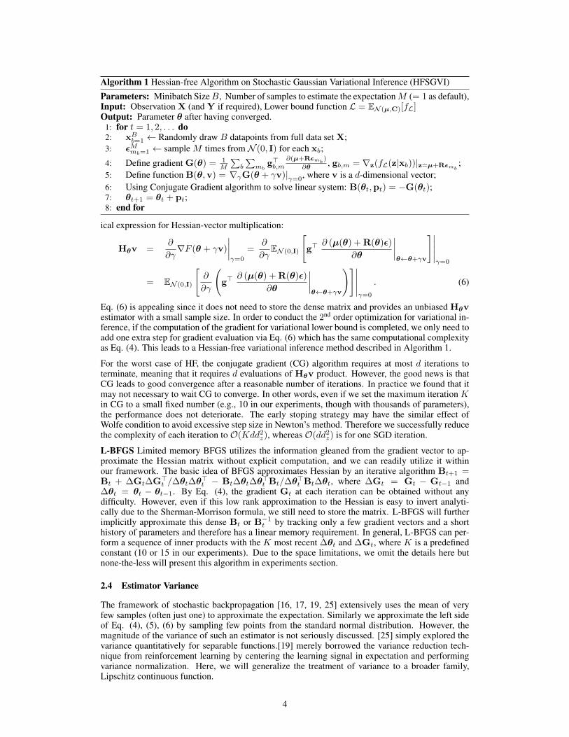
Algorithm 1 Hessian-free Algorithm on Stochastic Gaussian Variational Inference (HFSGVI)

Parameters: Minibatch SizeB, Number of samples to estimate the expectationM (= 1 as default),Input: Observation X (and Y if required), Lower bound function L = EN (µ,C)[fL]Output: Parameter θ after having converged.

1: for t = 1, 2, . . . do2: xBb=1 ← Randomly draw B datapoints from full data set X;3: εMmb=1 ← sample M times from N (0, I) for each xb;

4: Define gradient G(θ) = 1M

∑b

∑mb

g>b,m∂(µ+Rεmb )

∂θ , gb,m = ∇z(fL(z|xb))|z=µ+Rεmb;

5: Define function B(θ,v) = ∇γG(θ + γv)|γ=0, where v is a d-dimensional vector;6: Using Conjugate Gradient algorithm to solve linear system: B(θt,pt) = −G(θt);7: θt+1 = θt + pt;8: end for

ical expression for Hessian-vector multiplication:

Hθv =∂

∂γ∇F (θ + γv)

∣∣∣∣γ=0

=∂

∂γEN (0,I)

[g>

∂ (µ(θ) + R(θ)ε)

∂θ

∣∣∣∣θ←θ+γv

]∣∣∣∣∣γ=0

= EN (0,I)

[∂

∂γ

(g>

∂ (µ(θ) + R(θ)ε)

∂θ

∣∣∣∣θ←θ+γv

)]∣∣∣∣∣γ=0

. (6)

Eq. (6) is appealing since it does not need to store the dense matrix and provides an unbiased Hθvestimator with a small sample size. In order to conduct the 2nd order optimization for variational in-ference, if the computation of the gradient for variational lower bound is completed, we only need toadd one extra step for gradient evaluation via Eq. (6) which has the same computational complexityas Eq. (4). This leads to a Hessian-free variational inference method described in Algorithm 1.

For the worst case of HF, the conjugate gradient (CG) algorithm requires at most d iterations toterminate, meaning that it requires d evaluations of Hθv product. However, the good news is thatCG leads to good convergence after a reasonable number of iterations. In practice we found that itmay not necessary to wait CG to converge. In other words, even if we set the maximum iteration Kin CG to a small fixed number (e.g., 10 in our experiments, though with thousands of parameters),the performance does not deteriorate. The early stoping strategy may have the similar effect ofWolfe condition to avoid excessive step size in Newton’s method. Therefore we successfully reducethe complexity of each iteration to O(Kdd2z), whereas O(dd2z) is for one SGD iteration.

L-BFGS Limited memory BFGS utilizes the information gleaned from the gradient vector to ap-proximate the Hessian matrix without explicit computation, and we can readily utilize it withinour framework. The basic idea of BFGS approximates Hessian by an iterative algorithm Bt+1 =Bt + ∆Gt∆G>t /∆θt∆θ

>t − Bt∆θt∆θ

>t Bt/∆θ

>t Bt∆θt, where ∆Gt = Gt − Gt−1 and

∆θt = θt − θt−1. By Eq. (4), the gradient Gt at each iteration can be obtained without anydifficulty. However, even if this low rank approximation to the Hessian is easy to invert analyti-cally due to the Sherman-Morrison formula, we still need to store the matrix. L-BFGS will furtherimplicitly approximate this dense Bt or B−1t by tracking only a few gradient vectors and a shorthistory of parameters and therefore has a linear memory requirement. In general, L-BFGS can per-form a sequence of inner products with the K most recent ∆θt and ∆Gt, where K is a predefinedconstant (10 or 15 in our experiments). Due to the space limitations, we omit the details here butnone-the-less will present this algorithm in experiments section.

2.4 Estimator Variance

The framework of stochastic backpropagation [16, 17, 19, 25] extensively uses the mean of veryfew samples (often just one) to approximate the expectation. Similarly we approximate the left sideof Eq. (4), (5), (6) by sampling few points from the standard normal distribution. However, themagnitude of the variance of such an estimator is not seriously discussed. [25] simply explored thevariance quantitatively for separable functions.[19] merely borrowed the variance reduction tech-nique from reinforcement learning by centering the learning signal in expectation and performingvariance normalization. Here, we will generalize the treatment of variance to a broader family,Lipschitz continuous function.

4

Theorem 2 (Variance Bound). If f is an L-Lipschitz differentiable function and ε ∼ N (0, Idz ),then E[(f(ε)− E[f(ε)])2] ≤ L2π2

4 .

The proof of Theorem 2 (see supplementary) employs the properties of sub-Gaussian distributionsand the duplication trick that are commonly used in learning theory. Significantly, the result impliesa variance bound independent of the dimensionality of Gaussian variable. Note that from the proof,we can only obtain the E

[eλ(f(ε)−E[f(ε)])

]≤ eL

2λ2π2/8 for λ > 0. Though this result is enoughto illustrate the variance independence of dz , we can in fact tighten it to a sharper upper bound bya constant scalar, i.e. eλ

2L2/2, thus leading to the result of Theorem 2 with Var(f(ε)) ≤ L2. Ifall the results above hold for smooth (twice continuous and differentiable) functions with Lipschitzconstant L then it holds for all Lipschitz functions by a standard approximation argument. Thismeans the condition can be relaxed to Lipschitz continuous function.

Corollary 3 (Bias Bound). P(∣∣∣ 1M

∑Mm=1 f(εm)− E[f(ε)]

∣∣∣ ≥ t) ≤ 2e−2Mt2

π2L2 .

It is also worth mentioning that the significant corollary of Theorem 2 is probabilistic inequalityto measure the convergence rate of Monte Carlo approximation in our setting. This tail bound,together with variance bound, provides the theoretical guarantee for stochastic backpropagation onGaussian variables and provides an explanation for why a unique realization (M = 1) is enoughin practice. By reparametrization, Eq. (4), (5, (6) can be formulated as the expectation w.r.t theisotropic Gaussian distribution with identity covariance matrix leading to Algorithm 1. Thus wecan rein in the number of samples for Monte Carlo integration regardless dimensionality of latentvariables z. This seems counter-intuitive. However, we notice that larger L may require moresamples, and Lipschitz constants of different models vary greatly.

3 Application on Variational Auto-encoder

Note that our method is model free. If the loss function has the form of the expectation of a functionw.r.t latent Gaussian variables, we can directly use Algorithm 1. In this section, we put the emphasison a standard framework VAE model [17] that has been intensively researched; in particular, thefunction endows the logarithm form, thus bridging the gap between Hessian and fisher informationmatrix by expectation (see a survey [22] and reference therein).

3.1 Model Description

Suppose we have N i.i.d. observations X = {x(i)}Ni=1, where x(i) ∈ RD is a data vector that cantake either continuous or discrete values. In contrast to a standard auto-encoder model constructedby a neural network with a bottleneck structure, VAE describes the embedding process from theprospective of a Gaussian latent variable model. Specifically, each data point x follows a generativemodel pψ(x|z), where this process is actually a decoder that is usually constructed by a non-lineartransformation with unknown parameters ψ and a prior distribution pψ(z). The encoder or recog-nition model qφ(z|x) is used to approximate the true posterior pψ(z|x), where φ is similar to theparameter of variational distribution. As suggested in [16, 17, 25], multi-layered perceptron (MLP)is commonly considered as both the probabilistic encoder and decoder. We will later see that thisconstruction is equivalent to a variant deep neural networks under the constrain of unique realizationfor z. For this model and each datapoint, the variational lower bound on the marginal likelihood is,

log pψ(x(i)) ≥ Eqφ(z|x(i))[log pψ(x(i)|z)]−DKL(qφ(z|x(i))‖pψ(z)) = L(x(i)). (7)

We can actually write the KL divergence into the expectation term and denote (ψ,φ) as θ.By the previous discussion, this means that our objective is to solve the optimization problemarg maxθ

∑i L(x(i)) of full dataset variational lower bound. Thus L-BFGS or HF SGVI algorithm

can be implemented straightforwardly to estimate the parameters of both generative and recognitionmodels. Since the first term of reconstruction error appears in Eq. (7) with an expectation formon latent variable, [17, 25] used a small finite number M samples as Monte Carlo integration withreparameterization trick to reduce the variance. This is, in fact, drawing samples from the stan-dard normal distribution. In addition, the second term is the KL divergence between the variationaldistribution and the prior distribution, which acts as a regularizer.

5

3.2 Deep Neural Networks with Hybrid Hidden Layers

In the experiments, setting M = 1 can not only achieve excellent performance but also speed upthe program. In this special case, we discuss the relationship between VAE and traditional deepauto-encoder. For binary inputs, denote the output as y, we have log pψ(x|z) =

∑Dj=1 xj log yj +

(1−xj) log(1−yj), which is exactly the negative cross-entropy. It is also apparent that log pψ(x|z)is equivalent to negative squared error loss for continuous data. This means that maximizing thelower bound is roughly equal to minimizing the loss function of a deep neural network (see Figure1 in supplementary), except for different regularizers. In other words, the prior in VAE only im-poses a regularizer in encoder or generative model, while L2 penalty for all parameters is alwaysconsidered in deep neural nets. From the perspective of deep neural networks with hybrid hiddennodes, the model consists of two Bernoulli layers and one Gaussian layer. The gradient computationcan simply follow a variant of backpropagation layer by layer (derivation given in supplementary).To further see the rationale of setting M = 1, we will investigate the upper bound of the Lipschitzconstant under various activation functions in the next lemma. As Theorem 2 implies, the varianceof approximate expectation by finite samples mainly relies on the Lipschitz constant, rather thandimensionality. According to Lemma 4, imposing a prior or regularization to the parameter cancontrol both the model complexity and function smoothness. Lemma 4 also implies that we can getthe upper bound of the Lipschitz constant for the designed estimators in our algorithm.

Lemma 4. For a sigmoid activation function g in deep neural networks with one Gaussian layer z,z ∼ N (µ,C),C = R>R. Let z = µ + Rε, then the Lipschitz constant of g(Wi,(µ + Rε) + bi)is bounded by 1

4‖Wi,R‖2, where Wi, is ith row of weight matrix and bi is the ith element bias.Similarly, for hyperbolic tangent or softplus function, the Lipschitz constant is bounded by ‖Wi,R‖2.

4 Experiments

We apply our 2nd order stochastic variational inference to two different non-conjugate models. First,we consider a simple but widely used Bayesian logistic regression model, and compare with themost recent 1st order algorithm, doubly stochastic variational inference (DSVI) [28], designed forsparse variable selection with logistic regression. Then, we compare the performance of VAE modelwith our algorithms.

4.1 Bayesian Logistic Regression

Given a dataset {xi, yi}Ni=1, where each instance xi ∈ RD includes the default feature 1 andyi ∈ {−1, 1} is the binary label, the Bayesian logistic regression models the probability of out-puts conditional on features and the coefficients β with an imposed prior. The likelihood and theprior can usually take the form as

∏Ni=1 g(yix

>i β) and N (0,Λ) respectively, where g is sigmoid

function and Λ is a diagonal covariance matrix for simplicity. We can propose a variational Gaussiandistribution q(β|µ,C) to approximate the posterior of regression parameter. If we further assume adiagonal C, a factorized form

∏Dj=1 q(βj |µj , σj) is both efficient and practical for inference. Unlike

iteratively optimizing Λ and µ,C as in variational EM, [28] noticed that the calculation of the gra-dient w.r.t the lower bound indicates the updates of Λ can be analytically worked out by variationalparameters, thus resulting a new objective function for the representation of lower bound that onlyrelies onµ,C (details refer to [28]). We apply our algorithm to this variational logistic regression onthree appropriate datasets: DukeBreast and Leukemia are small size but high-dimensional forsparse logistic regression, and a9a which is large. See Table 1 for additional dataset descriptions.

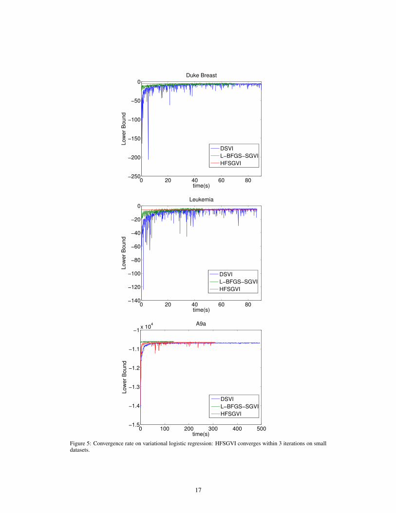
Fig. 5 shows the convergence of Gaussian variational lower bound for Bayesian logistic regressionin terms of running time. It is worth mentioning that the lower bound of HFSGVI converges within3 iterations on the small datasets DukeBreast and Leukemia. This is because all data pointsare fed to all algorithms and the HFSGVI uses a better approximation of the Hessian matrix toproceed 2nd order optimization. L-BFGS-SGVI also take less time to converge and yield slightlylarger lower bound than DSVI. In addition, as an SGD-based algorithm, it is clearly seen that DSVIis less stable for small datasets and fluctuates strongly even at the later optimized stage. For thelarge a9a, we observe that HFSGVI also needs 1000 iterations to reach a good lower bound andbecomes less stable than the other two algorithms. However, L-BFGS-SGVI performs the best

6

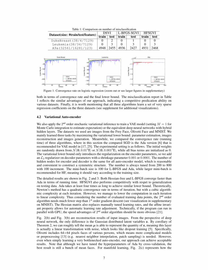
Table 1: Comparison on number of misclassification

Dataset(size: #train/test/feature) DSVI L-BFGS-SGVI HFSGVItrain test train test train test

DukeBreast(38/4/7129) 0 2 0 1 0 0Leukemia(38/34/7129) 0 3 0 3 0 3A9a(32561/16281/123) 4948 2455 4936 2427 4931 2468

0 20 40 60 80−250

−200

−150

−100

−50

0

time(s)

Lo

we

r B

ou

nd

Duke Breast

DSVI

L−BFGS−SGVI

HFSGVI

0 20 40 60 80−140

−120

−100

−80

−60

−40

−20

0

time(s)

Lo

we

r B

ou

nd

Leukemia

DSVI

L−BFGS−SGVI

HFSGVI

0 100 200 300 400 500−1.5

−1.4

−1.3

−1.2

−1.1

−1x 10

4

time(s)

Lo

we

r B

ou

nd

A9a

DSVI

L−BFGS−SGVI

HFSGVI

Figure 1: Convergence rate on logistic regression (zoom out or see larger figures in supplementary)

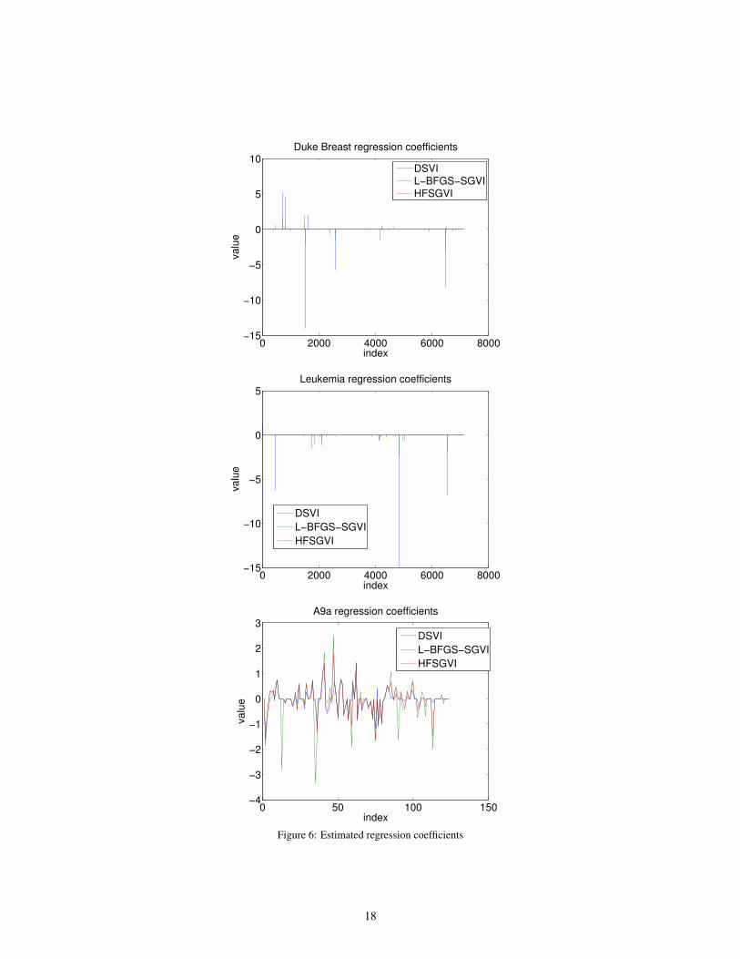
both in terms of convergence rate and the final lower bound. The misclassification report in Table1 reflects the similar advantages of our approach, indicating a competitive predication ability onvarious datasets. Finally, it is worth mentioning that all three algorithms learn a set of very sparseregression coefficients on the three datasets (see supplement for additional visualizations).

4.2 Variational Auto-encoder

We also apply the 2nd order stochastic variational inference to train a VAE model (settingM = 1 forMonte Carlo integration to estimate expectation) or the equivalent deep neural networks with hybridhidden layers. The datasets we used are images from the Frey Face, Olivetti Face and MNIST. Wemainly learned three tasks by maximizing the variational lower bound: parameter estimation, imagesreconstruction and images generation. Meanwhile, we compared the convergence rate (runningtime) of three algorithms, where in this section the compared SGD is the Ada version [6] that isrecommended for VAE model in [17, 25]. The experimental setting is as follows. The initial weightsare randomly drawn from N (0, 0.012I) or N (0, 0.0012I), while all bias terms are initialized as 0.The variational lower bound only introduces the regularization on the encoder parameters, so we addanL2 regularizer on decoder parameters with a shrinkage parameter 0.001 or 0.0001. The number ofhidden nodes for encoder and decoder is the same for all auto-encoder model, which is reasonableand convenient to construct a symmetric structure. The number is always tuned from 200 to 800with 100 increment. The mini-batch size is 100 for L-BFGS and Ada, while larger mini-batch isrecommended for HF, meaning it should vary according to the training size.

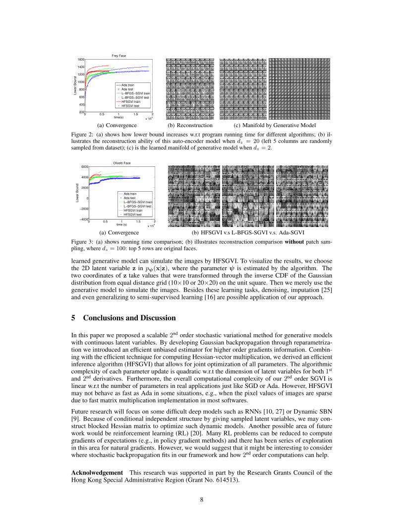
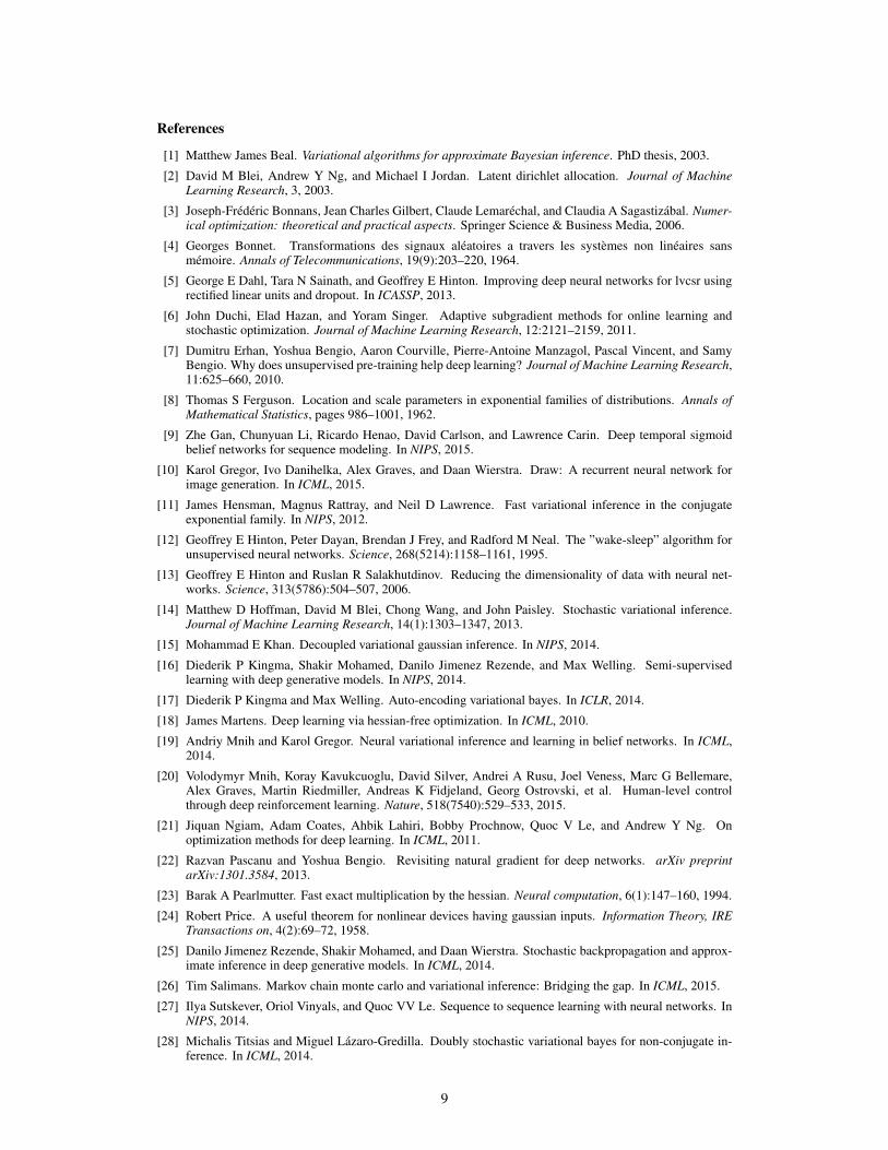
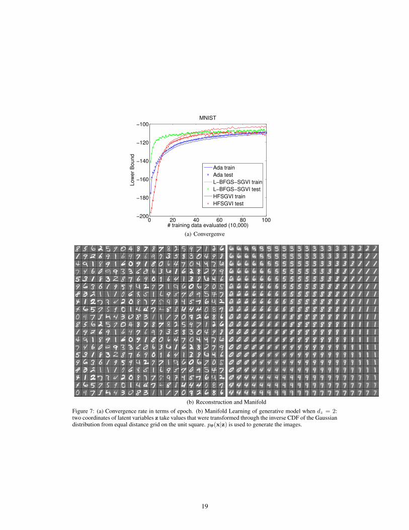
The detailed results are shown in Fig. 2 and 3. Both Hessian-free and L-BFGS converge faster thanAda in terms of running time. HFSGVI also performs competitively with respet to generalizationon testing data. Ada takes at least four times as long to achieve similar lower bound. Theoretically,Newton’s method has a quadratic convergence rate in terms of iteration, but with a cubic algorith-mic complexity at each iteration. However, we manage to lower the computation in each iterationto linear complexity. Thus considering the number of evaluated training data points, the 2nd orderalgorithm needs much fewer step than 1st order gradient descent (see visualization in supplementaryon MNIST). The Hessian matrix also replaces manually tuned learning rates, and the affine invari-ant property allows for automatic learning rate adjustment. Technically, if the program can run inparallel with GPU, the speed advantages of 2nd order algorithm should be more obvious [21].

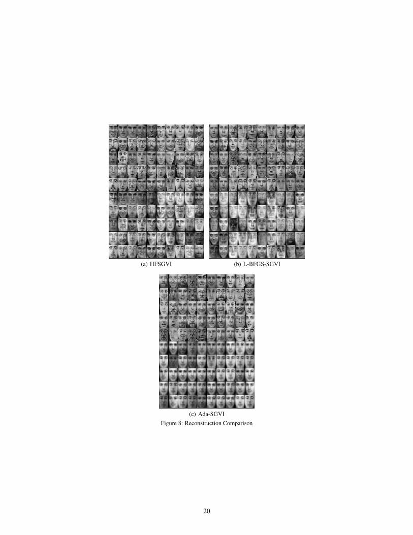
Fig. 2(b) and Fig. 3(b) are reconstruction results of input images. From the perspective of deepneural network, the only difference is the Gaussian distributed latent variables z. By corollary ofTheorem 2, we can roughly tell the mean µ is able to represent the quantity of z, meaning this layeris actually a linear transformation with noise, which looks like dropout training [5]. Specifically,Olivetti includes 64×64 pixels faces of various persons, which means more complicated modelsor preprocessing [13] (e.g. nearest neighbor interpolation, patch sampling) is needed. However,even when simply learning a very bottlenecked auto-encoder, our approach can achieve acceptableresults. Note that although we have tuned the hyperparameters of Ada by cross-validation, thebest result is still a bunch of mean faces. For manifold learning, Fig. 2(c) represents how the

7

0 0.5 1 1.5 2

x 104

200

400

600

800

1000

1200

1400

1600

time(s)

Lo

we

r B

ou

nd

Frey Face

Ada train

Ada test

L−BFGS−SGVI train

L−BFGS−SGVI test

HFSGVI train

HFSGVI test

(a) Convergence (b) Reconstruction (c) Manifold by Generative Model

Figure 2: (a) shows how lower bound increases w.r.t program running time for different algorithms; (b) il-lustrates the reconstruction ability of this auto-encoder model when dz = 20 (left 5 columns are randomlysampled from dataset); (c) is the learned manifold of generative model when dz = 2.

0 0.5 1 1.5 2

x 104

−4000

−2000

0

2000

4000

6000

time (s)

Lo

we

r B

ou

nd

Olivetti Face

Ada train

Ada test

L−BFGS−SGVI train

L−BFGS−SGVI test

HFSGVI train

HFSGVI test

(a) Convergence (b) HFSGVI v.s L-BFGS-SGVI v.s. Ada-SGVI

Figure 3: (a) shows running time comparison; (b) illustrates reconstruction comparison without patch sam-pling, where dz = 100: top 5 rows are original faces.

learned generative model can simulate the images by HFSGVI. To visualize the results, we choosethe 2D latent variable z in pψ(x|z), where the parameter ψ is estimated by the algorithm. Thetwo coordinates of z take values that were transformed through the inverse CDF of the Gaussiandistribution from equal distance grid (10×10 or 20×20) on the unit square. Then we merely use thegenerative model to simulate the images. Besides these learning tasks, denoising, imputation [25]and even generalizing to semi-supervised learning [16] are possible application of our approach.

5 Conclusions and Discussion

In this paper we proposed a scalable 2nd order stochastic variational method for generative modelswith continuous latent variables. By developing Gaussian backpropagation through reparametriza-tion we introduced an efficient unbiased estimator for higher order gradients information. Combin-ing with the efficient technique for computing Hessian-vector multiplication, we derived an efficientinference algorithm (HFSGVI) that allows for joint optimization of all parameters. The algorithmiccomplexity of each parameter update is quadratic w.r.t the dimension of latent variables for both 1st

and 2nd derivatives. Furthermore, the overall computational complexity of our 2nd order SGVI islinear w.r.t the number of parameters in real applications just like SGD or Ada. However, HFSGVImay not behave as fast as Ada in some situations, e.g., when the pixel values of images are sparsedue to fast matrix multiplication implementation in most softwares.

Future research will focus on some difficult deep models such as RNNs [10, 27] or Dynamic SBN[9]. Because of conditional independent structure by giving sampled latent variables, we may con-struct blocked Hessian matrix to optimize such dynamic models. Another possible area of futurework would be reinforcement learning (RL) [20]. Many RL problems can be reduced to computegradients of expectations (e.g., in policy gradient methods) and there has been series of explorationin this area for natural gradients. However, we would suggest that it might be interesting to considerwhere stochastic backpropagation fits in our framework and how 2nd order computations can help.

Acknolwedgement This research was supported in part by the Research Grants Council of theHong Kong Special Administrative Region (Grant No. 614513).

8

References

[1] Matthew James Beal. Variational algorithms for approximate Bayesian inference. PhD thesis, 2003.

[2] David M Blei, Andrew Y Ng, and Michael I Jordan. Latent dirichlet allocation. Journal of MachineLearning Research, 3, 2003.

[3] Joseph-Frederic Bonnans, Jean Charles Gilbert, Claude Lemarechal, and Claudia A Sagastizabal. Numer-ical optimization: theoretical and practical aspects. Springer Science & Business Media, 2006.

[4] Georges Bonnet. Transformations des signaux aleatoires a travers les systemes non lineaires sansmemoire. Annals of Telecommunications, 19(9):203–220, 1964.

[5] George E Dahl, Tara N Sainath, and Geoffrey E Hinton. Improving deep neural networks for lvcsr usingrectified linear units and dropout. In ICASSP, 2013.

[6] John Duchi, Elad Hazan, and Yoram Singer. Adaptive subgradient methods for online learning andstochastic optimization. Journal of Machine Learning Research, 12:2121–2159, 2011.

[7] Dumitru Erhan, Yoshua Bengio, Aaron Courville, Pierre-Antoine Manzagol, Pascal Vincent, and SamyBengio. Why does unsupervised pre-training help deep learning? Journal of Machine Learning Research,11:625–660, 2010.

[8] Thomas S Ferguson. Location and scale parameters in exponential families of distributions. Annals ofMathematical Statistics, pages 986–1001, 1962.

[9] Zhe Gan, Chunyuan Li, Ricardo Henao, David Carlson, and Lawrence Carin. Deep temporal sigmoidbelief networks for sequence modeling. In NIPS, 2015.

[10] Karol Gregor, Ivo Danihelka, Alex Graves, and Daan Wierstra. Draw: A recurrent neural network forimage generation. In ICML, 2015.

[11] James Hensman, Magnus Rattray, and Neil D Lawrence. Fast variational inference in the conjugateexponential family. In NIPS, 2012.

[12] Geoffrey E Hinton, Peter Dayan, Brendan J Frey, and Radford M Neal. The ”wake-sleep” algorithm forunsupervised neural networks. Science, 268(5214):1158–1161, 1995.

[13] Geoffrey E Hinton and Ruslan R Salakhutdinov. Reducing the dimensionality of data with neural net-works. Science, 313(5786):504–507, 2006.

[14] Matthew D Hoffman, David M Blei, Chong Wang, and John Paisley. Stochastic variational inference.Journal of Machine Learning Research, 14(1):1303–1347, 2013.

[15] Mohammad E Khan. Decoupled variational gaussian inference. In NIPS, 2014.

[16] Diederik P Kingma, Shakir Mohamed, Danilo Jimenez Rezende, and Max Welling. Semi-supervisedlearning with deep generative models. In NIPS, 2014.

[17] Diederik P Kingma and Max Welling. Auto-encoding variational bayes. In ICLR, 2014.

[18] James Martens. Deep learning via hessian-free optimization. In ICML, 2010.

[19] Andriy Mnih and Karol Gregor. Neural variational inference and learning in belief networks. In ICML,2014.

[20] Volodymyr Mnih, Koray Kavukcuoglu, David Silver, Andrei A Rusu, Joel Veness, Marc G Bellemare,Alex Graves, Martin Riedmiller, Andreas K Fidjeland, Georg Ostrovski, et al. Human-level controlthrough deep reinforcement learning. Nature, 518(7540):529–533, 2015.

[21] Jiquan Ngiam, Adam Coates, Ahbik Lahiri, Bobby Prochnow, Quoc V Le, and Andrew Y Ng. Onoptimization methods for deep learning. In ICML, 2011.

[22] Razvan Pascanu and Yoshua Bengio. Revisiting natural gradient for deep networks. arXiv preprintarXiv:1301.3584, 2013.

[23] Barak A Pearlmutter. Fast exact multiplication by the hessian. Neural computation, 6(1):147–160, 1994.

[24] Robert Price. A useful theorem for nonlinear devices having gaussian inputs. Information Theory, IRETransactions on, 4(2):69–72, 1958.

[25] Danilo Jimenez Rezende, Shakir Mohamed, and Daan Wierstra. Stochastic backpropagation and approx-imate inference in deep generative models. In ICML, 2014.

[26] Tim Salimans. Markov chain monte carlo and variational inference: Bridging the gap. In ICML, 2015.

[27] Ilya Sutskever, Oriol Vinyals, and Quoc VV Le. Sequence to sequence learning with neural networks. InNIPS, 2014.

[28] Michalis Titsias and Miguel Lazaro-Gredilla. Doubly stochastic variational bayes for non-conjugate in-ference. In ICML, 2014.

9

Appendix

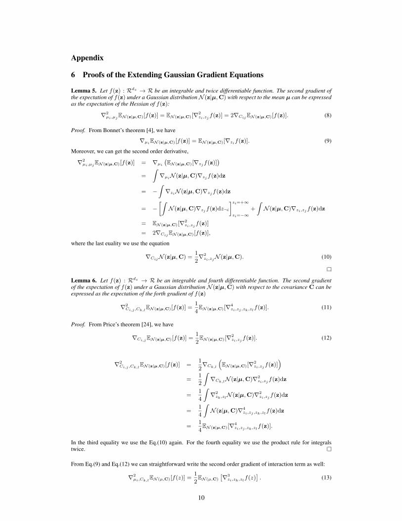
6 Proofs of the Extending Gaussian Gradient Equations

Lemma 5. Let f(z) : Rdz → R be an integrable and twice differentiable function. The second gradient ofthe expectation of f(z) under a Gaussian distributionN (z|µ,C) with respect to the mean µ can be expressedas the expectation of the Hessian of f(z):

∇2µi,µjEN (z|µ,C)[f(z)] = EN (z|µ,C)[∇2

zi,zjf(z)] = 2∇CijEN (z|µ,C)[f(z)]. (8)

Proof. From Bonnet’s theorem [4], we have

∇µiEN (z|µ,C)[f(z)] = EN (z|µ,C)[∇zif(z)]. (9)

Moreover, we can get the second order derivative,

∇2µi,µjEN (z|µ,C)[f(z)] = ∇µi

(EN (z|µ,C)[∇zjf(z)]

)=

∫∇µiN (z|µ,C)∇zjf(z)dz

= −∫∇ziN (z|µ,C)∇zjf(z)dz

= −[∫N (z|µ,C)∇zjf(z)dz¬i

]zi=+∞

zi=−∞+

∫N (z|µ,C)∇zi,zjf(z)dz

= EN (z|µ,C)[∇2zi,zjf(z)]

= 2∇CijEN (z|µ,C)[f(z)],

where the last euality we use the equation

∇CijN (z|µ,C) =1

2∇2zi,zjN (z|µ,C). (10)

Lemma 6. Let f(z) : Rdz → R be an integrable and fourth differentiable function. The second gradientof the expectation of f(z) under a Gaussian distribution N (z|µ,C) with respect to the covariance C can beexpressed as the expectation of the forth gradient of f(z)

∇2Ci,j ,Ck,lEN (z|µ,C)[f(z)] =

1

4EN (z|µ,C)[∇4

zi,zj ,zk,zlf(z)]. (11)

Proof. From Price’s theorem [24], we have

∇Ci,jEN (z|µ,C)[f(z)] =1

2EN (z|µ,C)[∇2

zi,zjf(z)]. (12)

∇2Ci,j ,Ck,lEN (z|µ,C)[f(z)] =

1

2∇Ck,l

(EN (z|µ,C)[∇2

zi,zjf(z)])

=1

2

∫∇Ck,lN (z|µ,C)∇2

zi,zjf(z)dz

=1

4

∫∇2zk,zlN (z|µ,C)∇2

zi,zjf(z)dz

=1

4

∫N (z|µ,C)∇4

zi,zj ,zk,zlf(z)dz

=1

4EN (z|µ,C)[∇4

zi,zj ,zk,zlf(z)].

In the third equality we use the Eq.(10) again. For the fourth equality we use the product rule for integralstwice.

From Eq.(9) and Eq.(12) we can straightforward write the second order gradient of interaction term as well:

∇2µi,Ck,lEN (µ,C)[f(z)] =

1

2EN (µ,C)

[∇3zi,zk,zlf(z)

]. (13)

10

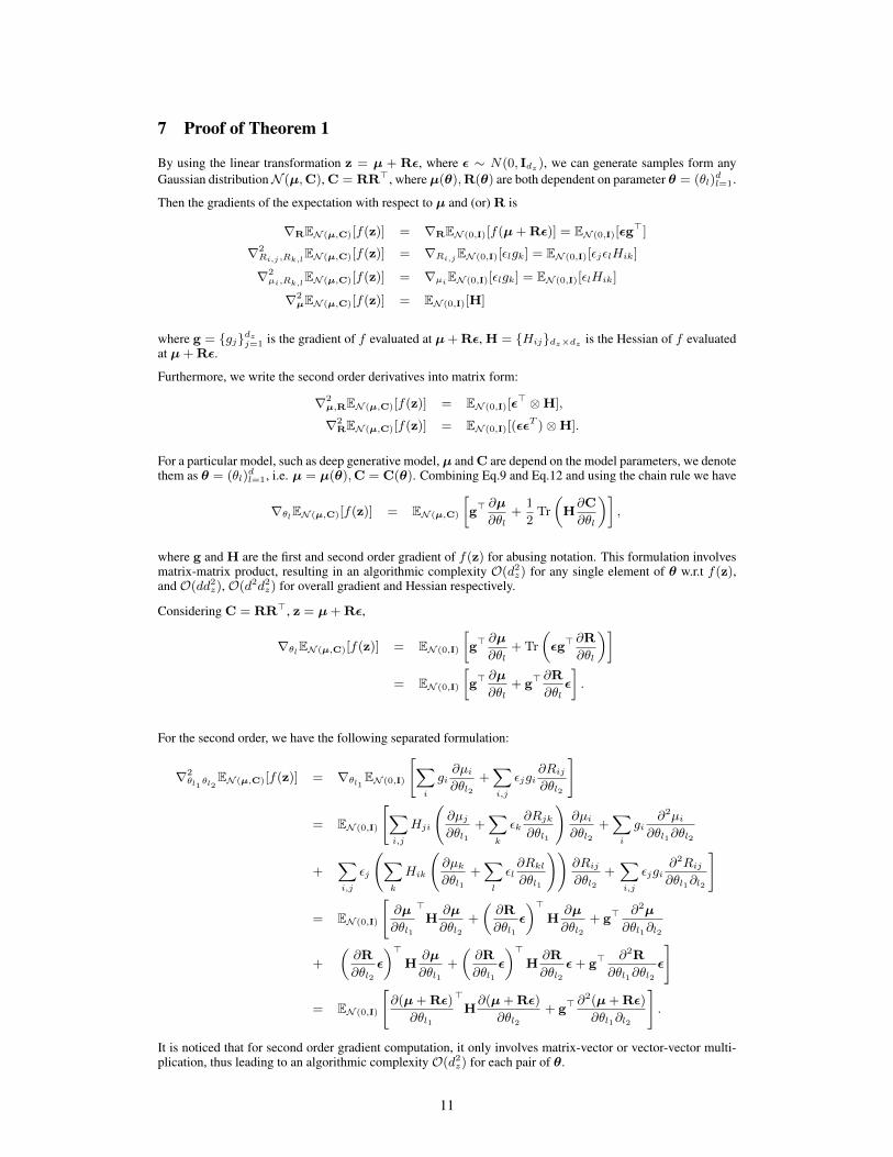
7 Proof of Theorem 1

By using the linear transformation z = µ + Rε, where ε ∼ N(0, Idz ), we can generate samples form anyGaussian distributionN (µ,C), C = RR>, where µ(θ),R(θ) are both dependent on parameter θ = (θl)

dl=1.

Then the gradients of the expectation with respect to µ and (or) R is

∇REN (µ,C)[f(z)] = ∇REN (0,I)[f(µ+Rε)] = EN (0,I)[εg>]

∇2Ri,j ,Rk,lEN (µ,C)[f(z)] = ∇Ri,jEN (0,I)[εlgk] = EN (0,I)[εjεlHik]

∇2µi,Rk,lEN (µ,C)[f(z)] = ∇µiEN (0,I)[εlgk] = EN (0,I)[εlHik]

∇2µEN (µ,C)[f(z)] = EN (0,I)[H]

where g = {gj}dzj=1 is the gradient of f evaluated at µ+Rε, H = {Hij}dz×dz is the Hessian of f evaluatedat µ+Rε.

Furthermore, we write the second order derivatives into matrix form:

∇2µ,REN (µ,C)[f(z)] = EN (0,I)[ε

> ⊗H],

∇2REN (µ,C)[f(z)] = EN (0,I)[(εε

T )⊗H].

For a particular model, such as deep generative model, µ and C are depend on the model parameters, we denotethem as θ = (θl)

dl=1, i.e. µ = µ(θ),C = C(θ). Combining Eq.9 and Eq.12 and using the chain rule we have

∇θlEN (µ,C)[f(z)] = EN (µ,C)

[g>

∂µ

∂θl+

1

2Tr

(H∂C

∂θl

)],

where g and H are the first and second order gradient of f(z) for abusing notation. This formulation involvesmatrix-matrix product, resulting in an algorithmic complexity O(d2z) for any single element of θ w.r.t f(z),and O(dd2z), O(d2d2z) for overall gradient and Hessian respectively.

Considering C = RR>, z = µ+Rε,

∇θlEN (µ,C)[f(z)] = EN (0,I)

[g>

∂µ

∂θl+Tr

(εg>

∂R

∂θl

)]= EN (0,I)

[g>

∂µ

∂θl+ g>

∂R

∂θlε

].

For the second order, we have the following separated formulation:

∇2θl1θl2

EN (µ,C)[f(z)] = ∇θl1EN (0,I)

[∑i

gi∂µi∂θl2

+∑i,j

εjgi∂Rij∂θl2

]

= EN (0,I)

[∑i,j

Hji

(∂µj∂θl1

+∑k

εk∂Rjk∂θl1

)∂µi∂θl2

+∑i

gi∂2µi

∂θl1∂θl2

+∑i,j

εj

(∑k

Hik

(∂µk∂θl1

+∑l

εl∂Rkl∂θl1

))∂Rij∂θl2

+∑i,j

εjgi∂2Rij∂θl1∂l2

]

= EN (0,I)

[∂µ

∂θl1

>H∂µ

∂θl2+

(∂R

∂θl1ε

)>H∂µ

∂θl2+ g>

∂2µ

∂θl1∂l2

+

(∂R

∂θl2ε

)>H∂µ

∂θl1+

(∂R

∂θl1ε

)>H∂R

∂θl2ε+ g>

∂2R

∂θl1∂θl2ε

]

= EN (0,I)

[∂(µ+Rε)

∂θl1

>H∂(µ+Rε)

∂θl2+ g>

∂2(µ+Rε)

∂θl1∂l2

].

It is noticed that for second order gradient computation, it only involves matrix-vector or vector-vector multi-plication, thus leading to an algorithmic complexity O(d2z) for each pair of θ.

11

One practical parametrization is C = diag{σ21 , ..., σ

2dz} or R = diag{σ1, ..., σdz}, which will reduce the

actual second order gradient computation complexity, albeit the same order of O(d2z). Then we have

∇θlEN (µ,C)[f(z)] = EN (0,I)

[g>

∂µ

∂θl+∑i

εigi∂σi∂θl

]

= EN (0,I)

[g>

∂µ

∂θl+ (ε� g)>

∂σ

∂θl

], (14)

∇2θl1θl2

EN (µ,C)[f(z)] = EN (0,I)

[∂µ

∂θl1

>H∂µ

∂θl2+

(ε� ∂σ

∂θl1

)>H∂µ

∂θl2+ g>

∂2µ

∂θl1∂θl2

+

(ε� ∂σ

∂θl2

)>H∂µ

∂θl1+

(ε� ∂σ

∂θl1

)>H

(ε� ∂σ

∂θl2

)+ (ε� g)>

∂2σ

∂θl1∂θl2

]= EN (0,I)

[(∂µ

∂θl1+ ε� ∂σ

∂θl1

)>H

(∂µ

∂θl2+ ε� ∂σ

∂θl2

)+ g>

(∂2µ

∂θl1∂θl2+∂2(ε� σ)

∂θl1∂θl2

)], (15)

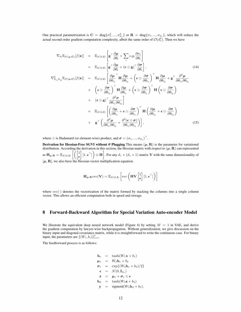
where � is Hadamard (or element-wise) product, and σ = (σ1, ..., σdz )>.

Derivation for Hessian-Free SGVI without θ Plugging This means (µ,R) is the parameter for variationaldistribution. According the derivation in this section, the Hessian matrix with respect to (µ,R) can represented

as Hµ,R = EN (0,I)

[([1ε

][1, ε>]

)⊗H

]. For any dz × (dz + 1) matrix V with the same dimensionality of

[µ,R], we also have the Hessian-vector multiplication equation.

Hµ,Rvec(V) = EN (0,I)

[vec

(HV

[1ε

][1, ε>]

)]

where vec(·) denotes the vectorization of the matrix formed by stacking the columns into a single columnvector. This allows an efficient computation both in speed and storage.

8 Forward-Backward Algorithm for Special Variation Auto-encoder Model

We illustrate the equivalent deep neural network model (Figure 4) by setting M = 1 in VAE, and derivethe gradient computation by lawyer-wise backpropagation. Without generalization, we give discussion on thebinary input and diagonal covariance matrix, while it is straightforward to write the continuous case. For binaryinput, the parameters are {(Wi, bi)}5i=1.

The feedforward process is as follows:

he = tanh(W1x+ b1)

µe = W2he + b2

σe = exp{(W3he + b3)/2}ε ∼ N (0, Idz )

z = µe + σe � ε

hd = tanh(W4z+ b4)

y = sigmoid(W5hd + b5).

12

Input:  x

Output:  y

hd

z

he

W1,  b1

(W2,  b2), (W3,  b3)

W4,  b4

W5,  b5 Hidden  decoder  layer

Hidden  encoder  layer

Gaussian  latent  layer

he

Sigma mu

(W2,  b2)   (W3,  b3)

N(                                ,                              ) ~

(W5,  b5),  (W6,  b6)  if  x  is  con?nuous.

Figure 4: Auto-encoder Model by Deep Neural Nets.

Considering the cross-entropy loss function, the backward process for gradient backpropagation computationis:

δ5 = x� (1− y)− (1− x)� y

∇W5 = δ5h>d , ∇b5 = δ5

δ4 = (W>5 δ5)� (1− hd � hd)

∇W4 = δ4z>, ∇b4 = δ4

δ3 = 0.5 ∗ [(W>4 δ4)� (z− µe) + 1− σ2e ]

∇W3 = δ3h>e , ∇b3 = δ3

δ2 = W>4 δ4 − µe

∇W2 = δ2h>e , ∇b2 = δ2

δ1 = (W>2 δ2 +W>3 δ3)� (1− he � he)

∇W1 = δ1x>, ∇b1 = δ1.

Notice that when we compute the differences δ2, δ3, we also include the prior term which acts as the roleof regularization penalty. In addition, we can add the L2 penalty to the weight matrix as well. The onlymodification is to change the expression of∇Wi by adding λWi, where λ is a tunable hyper-parameter.

9 R-Operator Derivation

Define Rv{f(θ)} = ∂∂γf(θ + γv)

∣∣∣γ=0

, then Hθv = Rv{∇θF (θ)}. First, mapping v to

{R{Wi},R{bi}}5i=1. Then, we derive the Hv to {R{DWi},R{Dbi}}5i=1, where D-operator means takederivative with respect to objective function.

Denote si =Wiu+ bi, where u can represent any vector used in neural networks.Forward Pass:

R{s1} = R{W1}x+R{b1} ( SinceR{x} = 0)

R{he} = R{s1} tanh′(s1)R{µe} = R{s2} = R{W2}he +W2R{he}+R{b2}R{s3} = R{W3}he +W3R{he}+R{b3}R{σe} = R{s3} exp{s3/2} ( Since (ex)′ = ex)

R{z} = R{µe}+R{σe} � ε

R{s4} = R{W4}z+W4R{z}+R{b4}R{hd} = R{s4} tanh′(s4)R{s5} = R{W5}hd +W5R{hd}+R{b5}R{y} = R{s5}sigmoid′(s5)

13

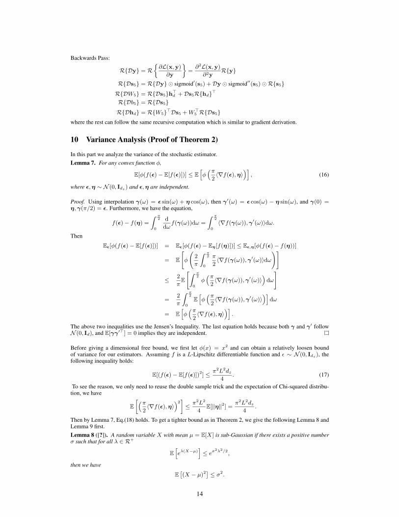
Backwards Pass:

R{Dy} = R{∂L(x,y)∂y

}=∂2L(x,y)∂2y

R{y}

R{Ds5} = R{Dy} � sigmoid′(s5) +Dy � sigmoid′′(s5)�R{s5}

R{DW5} = R{Ds5}h>d +Ds5R{hd}>

R{Db5} = R{Ds5}

R{Dhd} = R{W5}>Ds5 +W>5 R{Ds5}where the rest can follow the same recursive computation which is similar to gradient derivation.

10 Variance Analysis (Proof of Theorem 2)

In this part we analyze the variance of the stochastic estimator.Lemma 7. For any convex function φ,

E[φ(f(ε)− E[f(ε)])] ≤ E[φ(π2〈∇f(ε),η〉

)], (16)

where ε,η ∼ N (0, Idz ) and ε,η are independent.

Proof. Using interpolation γ(ω) = ε sin(ω) + η cos(ω), then γ′(ω) = ε cos(ω) − η sin(ω), and γ(0) =η,γ(π/2) = ε. Furthermore, we have the equation,

f(ε)− f(η) =∫ π

2

0

d

dωf(γ(ω))dω =

∫ π2

0

〈∇f(γ(ω)),γ′(ω)〉dω.

Then

Eε[φ(f(ε)− E[f(ε)])] = Eε[φ(f(ε)− Eη[f(η)])] ≤ Eε,η[φ(f(ε)− f(η))]

= E

[φ

(2

π

∫ π2

0

π

2〈∇f(γ(ω)),γ′(ω)〉dω

)]

≤ 2

πE

[∫ π2

0

φ(π2〈∇f(γ(ω)),γ′(ω)〉

)dω

]

=2

π

∫ π2

0

E[φ(π2〈∇f(γ(ω)),γ′(ω)〉

)]dω

= E[φ(π2〈∇f(ε),η〉

)].

The above two inequalities use the Jensen’s Inequality. The last equation holds because both γ and γ′ followN (0, Id), and E[γγ′>] = 0 implies they are independent.

Before giving a dimensional free bound, we first let φ(x) = x2 and can obtain a relatively loosen boundof variance for our estimators. Assuming f is a L-Lipschitz differentiable function and ε ∼ N (0, Idz ), thefollowing inequality holds:

E[(f(ε)− E[f(ε)])2] ≤ π2L2dz4

. (17)

To see the reason, we only need to reuse the double sample trick and the expectation of Chi-squared distribu-tion, we have

E[(π

2〈∇f(ε),η〉

)2]≤ π2L2

4E[‖η‖2] = π2L2dz

4.

Then by Lemma 7, Eq.(18) holds. To get a tighter bound as in Theorem 2, we give the following Lemma 8 andLemma 9 first.Lemma 8 ([?]). A random variable X with mean µ = E[X] is sub-Gaussian if there exists a positive numberσ such that for all λ ∈ R+

E[eλ(X−µ)

]≤ eσ

2λ2/2,

then we have

E[(X − µ)2

]≤ σ2.

14

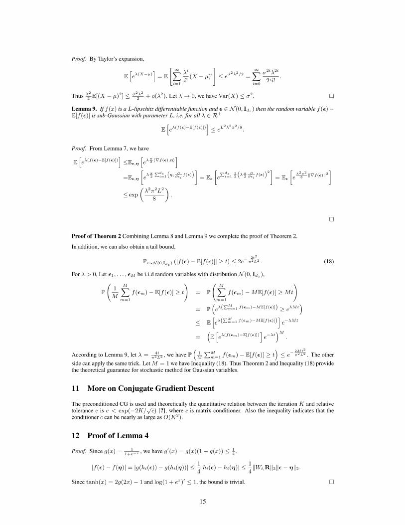
Proof. By Taylor’s expansion,

E[eλ(X−µ)

]= E

[∞∑i=1

λi

i!(X − µ)i

]≤ eσ

2λ2/2 =

∞∑i=0

σ2iλ2i

2ii!.

Thus λ2

2E[(X − µ)2] ≤ σ2λ2

2+ o(λ2). Let λ→ 0, we have Var(X) ≤ σ2.

Lemma 9. If f(x) is a L-lipschitz differentiable function and ε ∈ N (0, Idz ) then the random variable f(ε)−E[f(ε)] is sub-Gaussian with parameter L, i.e. for all λ ∈ R+

E[eλ(f(ε)−E[f(ε)])

]≤ eL

2λ2π2/8.

Proof. From Lemma 7, we have

E[eλ(f(ε)−E[f(ε)])

]≤Eε,η

[eλ

π2〈∇f(ε),η〉

]=Eε,η

[eλπ

2

∑dzi=1

(ηi

∂∂εi

f(ε))]

= Eε

[e∑dzi=1

12

(λπ

2∂∂εi

f(ε))2]

= Eε

[eλ2π2

8‖∇f(ε)‖2

]≤ exp

(λ2π2L2

8

).

Proof of Theorem 2 Combining Lemma 8 and Lemma 9 we complete the proof of Theorem 2.

In addition, we can also obtain a tail bound,

Pε∼N (0,Idz )(|f(ε)− E[f(ε)]| ≥ t) ≤ 2e

− 2t2

π2L2 . (18)

For λ > 0, Let ε1, . . . , εM be i.i.d random variables with distributionN (0, Idz ),

P

(1

M

M∑m=1

f(εm)− E[f(ε)] ≥ t

)= P

(M∑m=1

f(εm)−ME[f(ε)] ≥Mt

)= P

(eλ(

∑Mm=1 f(εm)−ME[f(ε)]) ≥ eλMt

)≤ E

[eλ(

∑Mm=1 f(εm)−ME[f(ε)])

]e−λMt

=(E[eλ(f(εm)−E[f(ε)])

]e−λt

)M.

According to Lemma 9, let λ = 4tπ2L2 , we have P

(1M

∑Mm=1 f(εm)− E[f(ε)] ≥ t

)≤ e− 2Mt2

π2L2 . The otherside can apply the same trick. LetM = 1 we have Inequality (18). Thus Theorem 2 and Inequality (18) providethe theoretical guarantee for stochastic method for Gaussian variables.

11 More on Conjugate Gradient Descent

The preconditioned CG is used and theoretically the quantitative relation between the iteration K and relativetolerance e is e < exp(−2K/

√c) [?], where c is matrix conditioner. Also the inequality indicates that the

conditioner c can be nearly as large as O(K2).

12 Proof of Lemma 4

Proof. Since g(x) = 11+e−x , we have g′(x) = g(x)(1− g(x)) ≤ 1

4.

|f(ε)− f(η)| = |g(hi(ε))− g(hi(η))| ≤1

4|hi(ε)− hi(η)| ≤

1

4‖Wi,R‖2‖ε− η‖2.

Since tanh(x) = 2g(2x)− 1 and log(1 + ex)′ ≤ 1, the bound is trivial.

15

13 Experiments

All the experiments are conducted on a 3.2GHz CPU computer with X-Intel 32G RAM. For fair comparison,the algorithms and datasets we referred to as the baseline remain the same as in the previously cited work andsoftware was downloaded from the website of relevant papers.

Datasets DukeBreast, Leukemia and A9a are downloaded from http://www.csie.ntu.edu.tw/˜cjlin/libsvmtools/datasets/binary.html. Datasets Frey Face, Olivetti Face and MNIST aredownloaded from http://www.cs.nyu.edu/˜roweis/data.html.

13.1 Variational logistic regression

The optimized lower bound function when the covariance matrix C is diagonal is as following.

L(µ,σ) = Ez∼N (0,I)[log l(µ+ σ � z)] +1

2

d∑i=1

logσ2i

σ2i + µ2

i

,

where l is the likelihood function.

The results are shown in Fig. 5 and Fig. 6.

13.2 Variational Auto-encoder

The results are shown in Fig. 7 and Fig. 8.

16

0 20 40 60 80−250

−200

−150

−100

−50

0

time(s)

Lo

we

r B

ou

nd

Duke Breast

DSVI

L−BFGS−SGVI

HFSGVI

0 20 40 60 80−140

−120

−100

−80

−60

−40

−20

0

time(s)

Lo

we

r B

ou

nd

Leukemia

DSVI

L−BFGS−SGVI

HFSGVI

0 100 200 300 400 500−1.5

−1.4

−1.3

−1.2

−1.1

−1x 10

4

time(s)

Lo

we

r B

ou

nd

A9a

DSVI

L−BFGS−SGVI

HFSGVI

Figure 5: Convergence rate on variational logistic regression: HFSGVI converges within 3 iterations on smalldatasets.

17

0 2000 4000 6000 8000−15

−10

−5

0

5

10

index

va

lue

Duke Breast regression coefficients

DSVIL−BFGS−SGVIHFSGVI

0 2000 4000 6000 8000−15

−10

−5

0

5

index

va

lue

Leukemia regression coefficients

DSVI

L−BFGS−SGVI

HFSGVI

0 50 100 150−4

−3

−2

−1

0

1

2

3

index

va

lue

A9a regression coefficients

DSVI

L−BFGS−SGVI

HFSGVI

Figure 6: Estimated regression coefficients

18

0 20 40 60 80 100−200

−180

−160

−140

−120

−100

# training data evaluated (10,000)

Low

er

Bo

un

d

MNIST

Ada train

Ada test

L−BFGS−SGVI train

L−BFGS−SGVI test

HFSGVI train

HFSGVI test

(a) Convergenve

(b) Reconstruction and Manifold

Figure 7: (a) Convergence rate in terms of epoch. (b) Manifold Learning of generative model when dz = 2:two coordinates of latent variables z take values that were transformed through the inverse CDF of the Gaussiandistribution from equal distance grid on the unit square. pθ(x|z) is used to generate the images.

19

(a) HFSGVI (b) L-BFGS-SGVI

(c) Ada-SGVI

Figure 8: Reconstruction Comparison

20