Stochastic Variational Method and Viscous Hydrodynamicsbrat/Home-NeD/talks_pdf/Sep1/Kodama.pdf ·...
54
Stochastic Variational Method and Viscous Hydrodynamics 1 A tentative approach
Transcript of Stochastic Variational Method and Viscous Hydrodynamicsbrat/Home-NeD/talks_pdf/Sep1/Kodama.pdf ·...

Stochastic Variational
Method and Viscous
Hydrodynamics
1
A tentative approach
Stochastic Variational
Method and Viscous
Hydrodynamics
T. Koide (小出 知威)
T. Kodama (小玉 剛)
TK and TK, arXiv:1108.01242
Federal Univ. of Rio de Janeiro
Stochastic Variational
Method and Viscous
Hydrodynamics
T. Koide (小出 知威)
T. Kodama (小玉 剛)
TK and TK, arXiv:1108.01243
Federal Univ. of Rio de Janeiro
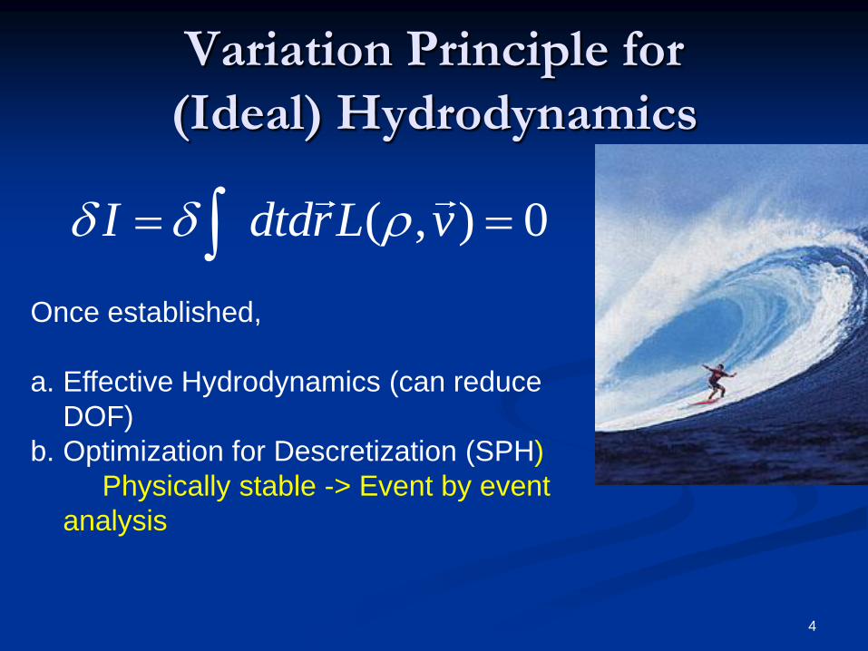
Variation Principle for
(Ideal) Hydrodynamics
Once established,
a. Effective Hydrodynamics (can reduce
DOF)
b. Optimization for Descretization (SPH)
Physically stable -> Event by event
analysis
4
( , ) 0I dtdrL v
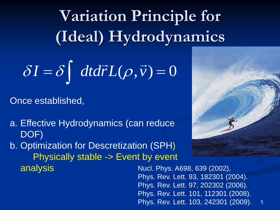
Variation Principle for
(Ideal) Hydrodynamics
Once established,
a. Effective Hydrodynamics (can reduce
DOF)
b. Optimization for Descretization (SPH)
Physically stable -> Event by event
analysis
5
( , ) 0I dtdrL v
Nucl. Phys. A698, 639 (2002),
Phys. Rev. Lett. 93, 182301 (2004).
Phys. Rev. Lett. 97, 202302 (2006).
Phys. Rev. Lett. 101, 112301 (2008).
Phys. Rev. Lett. 103, 242301 (2009).
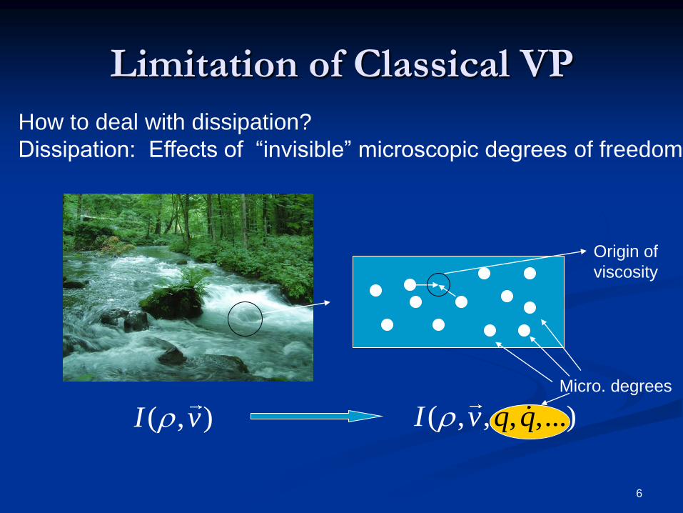
Limitation of Classical VP
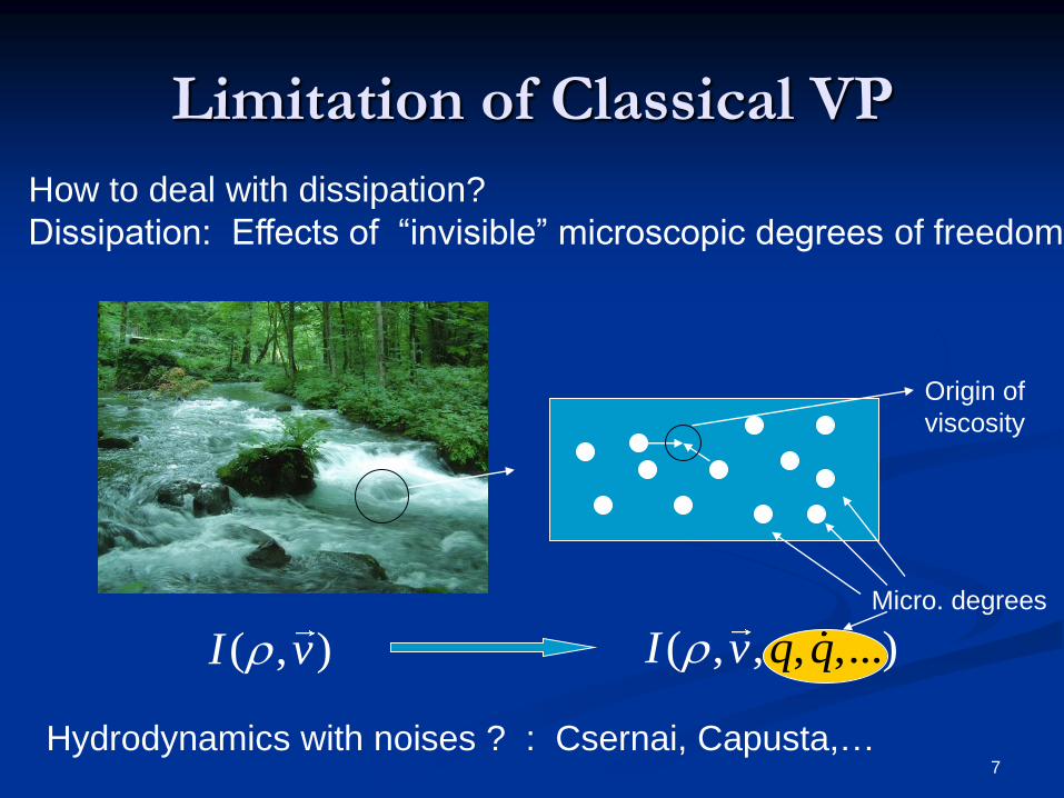
How to deal with dissipation?
Dissipation: Effects of “invisible” microscopic degrees of freedom
( , )I v , ,, ).., .(I qv qMicro. degrees
Origin of
viscosity
6
Limitation of Classical VP
How to deal with dissipation?
Dissipation: Effects of “invisible” microscopic degrees of freedom
( , )I v , ,, ).., .(I qv qMicro. degrees
Origin of
viscosity
7
Hydrodynamics with noises ? : Csernai, Capusta,…
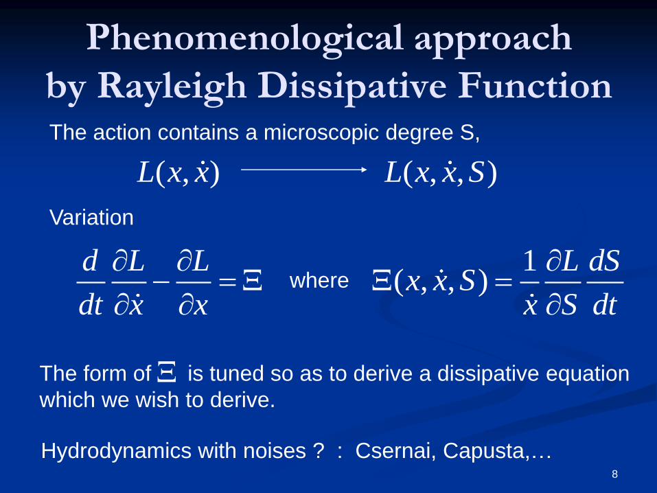
Phenomenological approach
by Rayleigh Dissipative FunctionThe action contains a microscopic degree S,
( , )L x x ( , , )L x x S
Variation
d L L
dt x x
1( , , )
L dSx x S
x S dt
where
The form of is tuned so as to derive a dissipative equation
which we wish to derive.
8
Hydrodynamics with noises ? : Csernai, Capusta,…
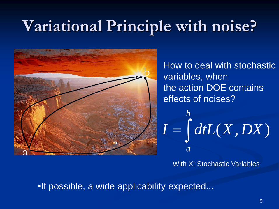
Variational Principle with noise?
( , )
b
a
I dtL X DX a
bHow to deal with stochastic
variables, when
the action DOE contains
effects of noises?
•If possible, a wide applicability expected...
9
With X: Stochastic Variables
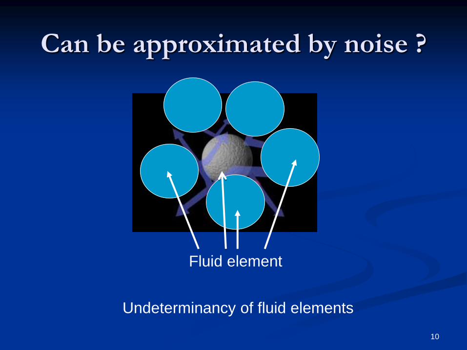
Can be approximated by noise ?
Fluid element
Undeterminancy of fluid elements
10
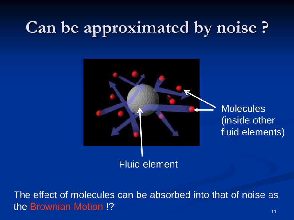
Can be approximated by noise ?
Fluid element
Molecules
(inside other
fluid elements)
The effect of molecules can be absorbed into that of noise as
the Brownian Motion !?11
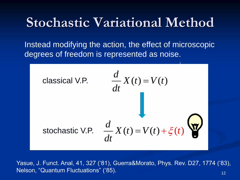
Stochastic Variational Method
Instead modifying the action, the effect of microscopic
degrees of freedom is represented as noise.
( ) ( )d
X t V tdt
( ( )) ( )d
X t V t tdt
classical V.P.
stochastic V.P.
Yasue, J. Funct. Anal, 41, 327 („81), Guerra&Morato, Phys. Rev. D27, 1774 („83),
Nelson, “Quantum Fluctuations” („85).12
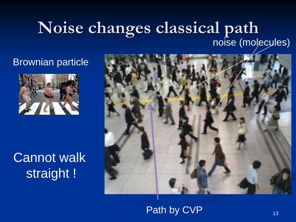
Path by CVP
Noise changes classical path
Cannot walk
straight !
noise (molecules)
Brownian particle
13
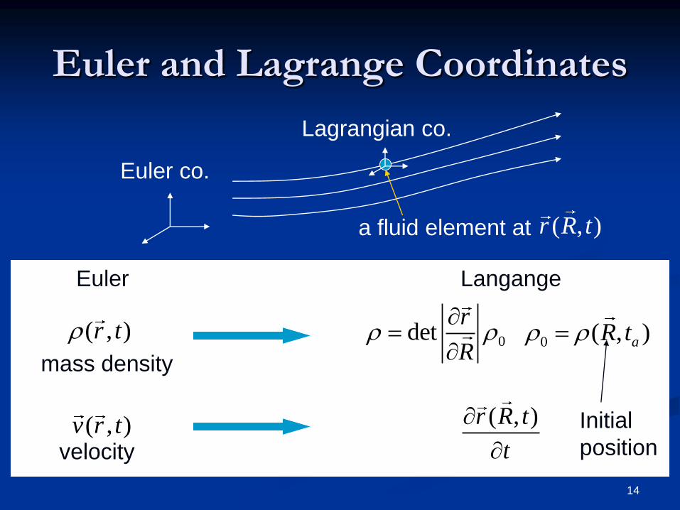
Euler and Lagrange Coordinates
0 ( , )aR t
( , )v r t
( , )r t
Euler co.
Lagrangian co.
( , )r R t
( , )r R t
t
a fluid element at
0detr
R
Euler Langange
mass density
velocity
Initial
position
14
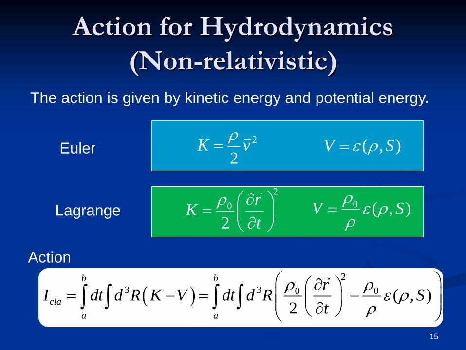
Action for Hydrodynamics
(Non-relativistic)
The action is given by kinetic energy and potential energy.
2
2K v
( , )V S
2
0
2
rK
t
0 ( , )V S
Euler
Lagrange
2
3 3 0 0 ( , )2
b b
cla
a a
rI dt d R K V dt d R S
t
Action
15
Classical variational method
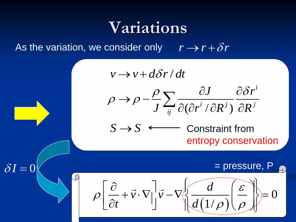
VariationsAs the variation, we consider only r r r
S S
/v v d r dt
( / )
i
i j jij
J r
J r R R
Constraint from
entropy conservation
0I
0
1/
dv v
t d
= pressure, P
17
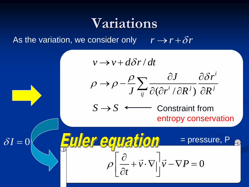
VariationsAs the variation, we consider only r r r
S S
/v v d r dt
( / )
i
i j jij
J r
J r R R
Constraint from
entropy conservation
0I
0v v Pt
= pressure, P
18
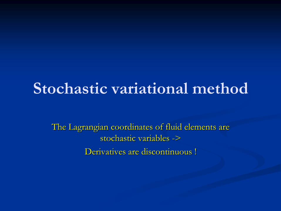
Stochastic variational method
The Lagrangian coordinates of fluid elements are
stochastic variables ->
Derivatives are discontinuous !
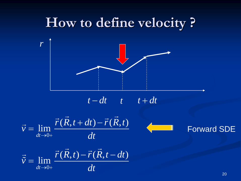
How to define velocity ?
r
t t dtt dt
0
( , ) ( , )lim
dt
r R t dt r R tv
dt
0
( , ) ( , )lim
dt
r R t r R t dtv
dt
Forward SDE
20
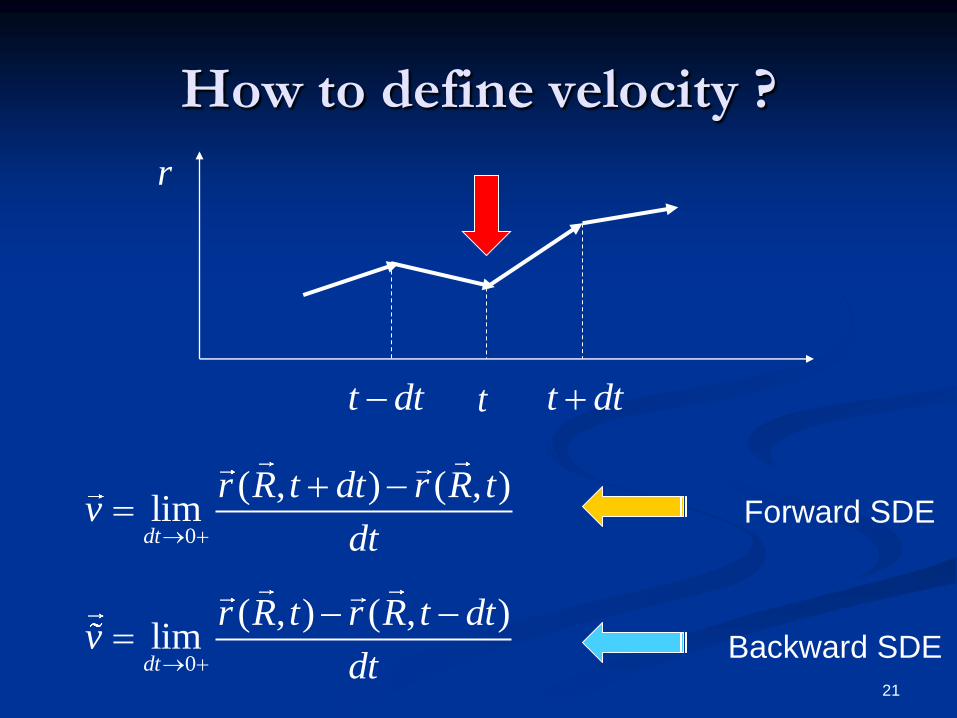
How to define velocity ?
r
t t dtt dt
0
( , ) ( , )lim
dt
r R t dt r R tv
dt
0
( , ) ( , )lim
dt
r R t r R t dtv
dt
Forward SDE
Backward SDE
21
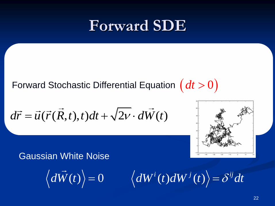
Forward SDE
( ( , ), ) 2 ( )dr u r R t t dt dW t
0dt Forward Stochastic Differential Equation
( ) 0dW t ( ) ( )i j ijdW t dW t dt
Gaussian White Noise
22
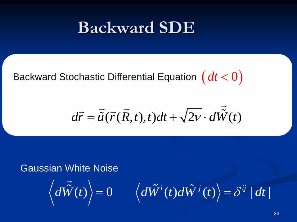
Backward SDE
( ( , ), ) 2 ( )dr u r R t t dt dW t
0dt
( ) 0dW t ( ) ( ) | |i j ijdW t dW t dt
Gaussian White Noise
Backward Stochastic Differential Equation
23
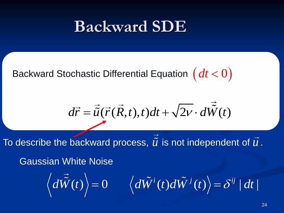
Backward SDE
( ( , ), ) 2 ( )dr u r R t t dt dW t
0dt
( ) 0dW t ( ) ( ) | |i j ijdW t dW t dt
Gaussian White Noise
Backward Stochastic Differential Equation
24
To describe the backward process, is not independent of .u u
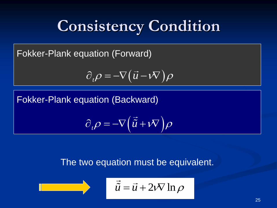
Consistency Condition
Fokker-Plank equation (Forward)
t u
Fokker-Plank equation (Backward)
t u
The two equation must be equivalent.
2 lnu u 25
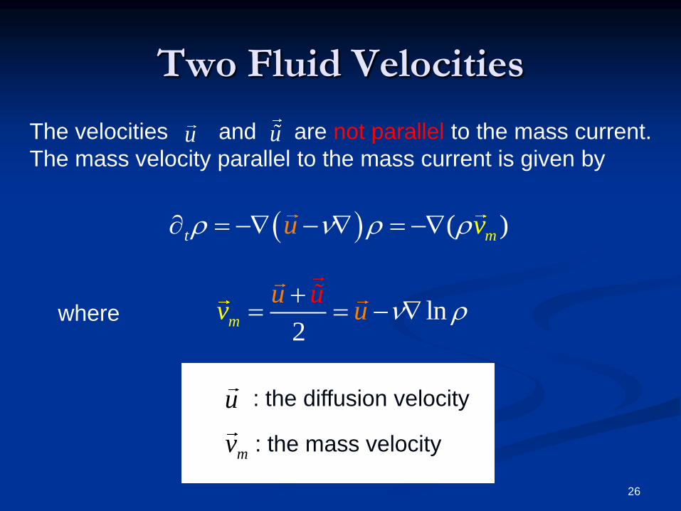
Two Fluid Velocities
The velocities and are not parallel to the mass current.
The mass velocity parallel to the mass current is given by u u
( )t mu v
where ln2
mvu u
u
mv
u : the diffusion velocity
: the mass velocity
26
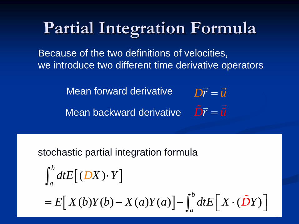
Partial Integration Formula
Mean forward derivative D ur
Mean backward derivative rD u
stochastic partial integration formula
( )
( ) ( ) ( ) ( ) ( )
b
a
b
a
dtE X Y
E X b Y b X a Y a X DdtE
D
Y
Because of the two definitions of velocities,
we introduce two different time derivative operators
27
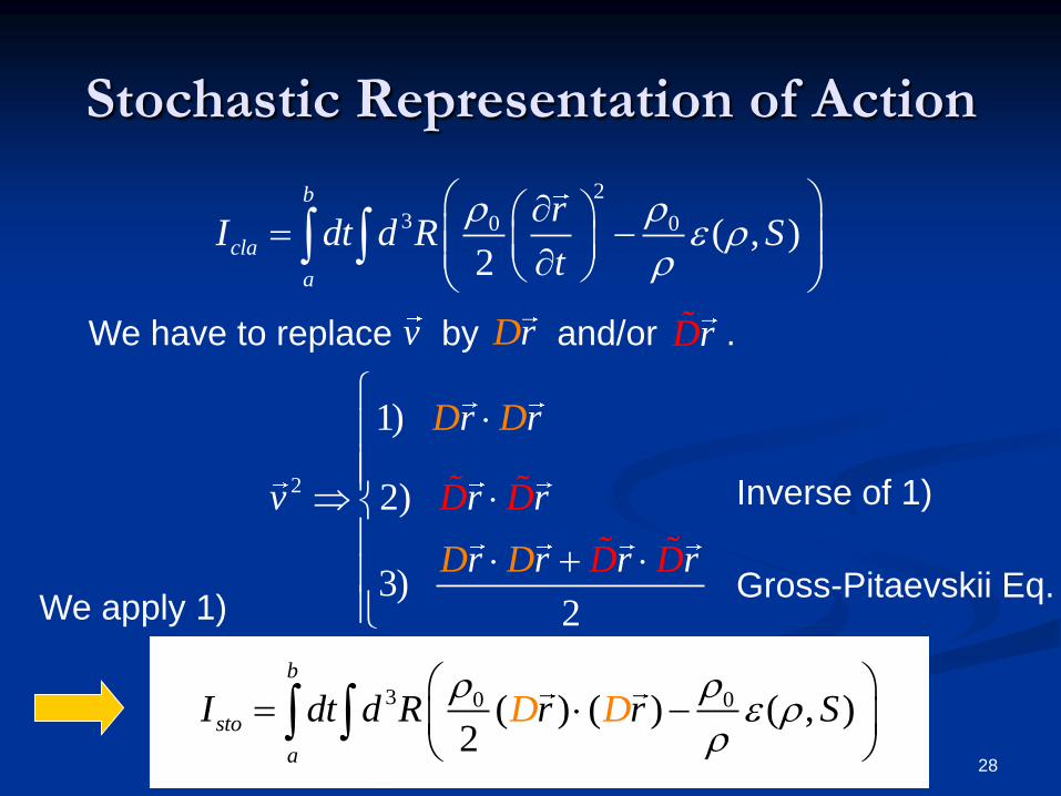
Stochastic Representation of Action
2
3 0 0 ( , )2
b
cla
a
rI dt d R S
t
3 0 0( ) ( ) ( , )2
b
sto
a
I dt d R r rD SD
We have to replace by and/or .v Dr rD
2
1)
2)
3)2
D D
D
r r
v r r
r r
D D
DrD rD
Gross-Pitaevskii Eq.
Inverse of 1)
We apply 1)
28
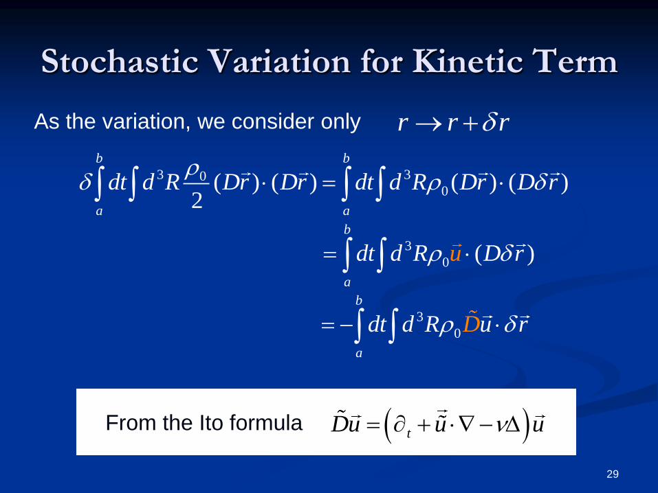
Stochastic Variation for Kinetic Term
As the variation, we consider only r r r
3 300( ) ( ) ( ) ( )
2
b b
a a
dt d R Dr Dr dt d R Dr D r
3
0 ( )
b
a
dt d R D ru
3
0
b
a
dt d R u rD
tDu u u From the Ito formula
29
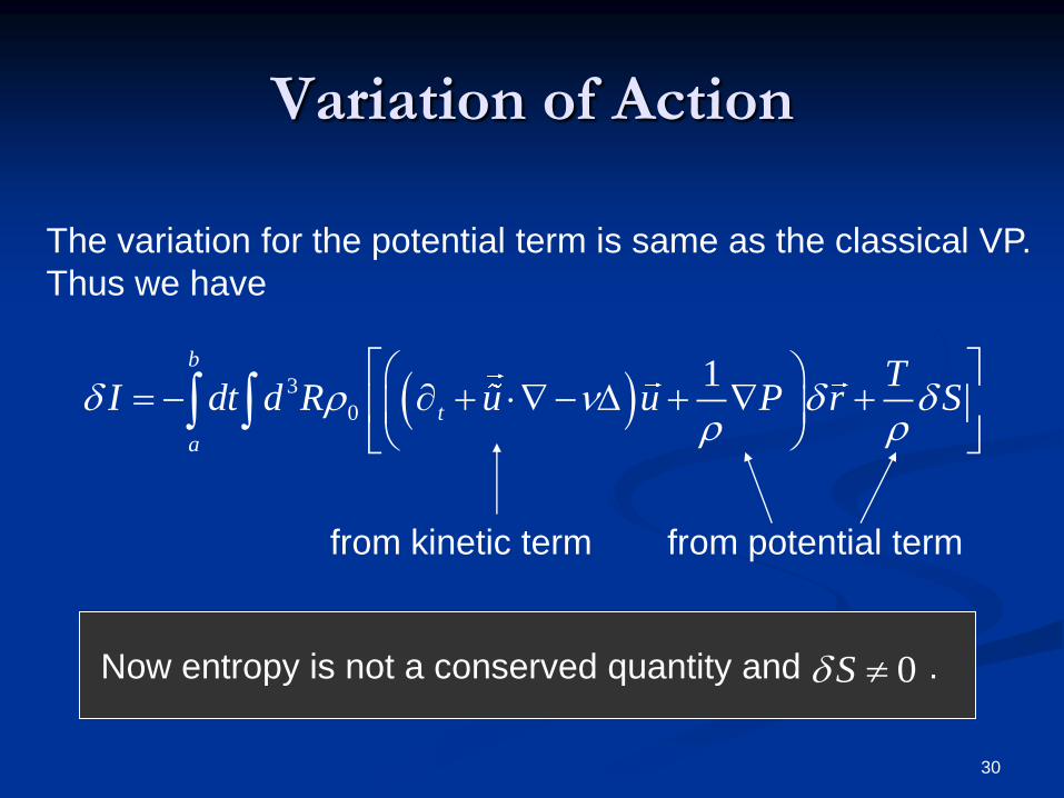
Variation of Action
3
0
1b
t
a
TI dt d R u u P r S
Now entropy is not a conserved quantity and .0S
The variation for the potential term is same as the classical VP.
Thus we have
from kinetic term from potential term
30
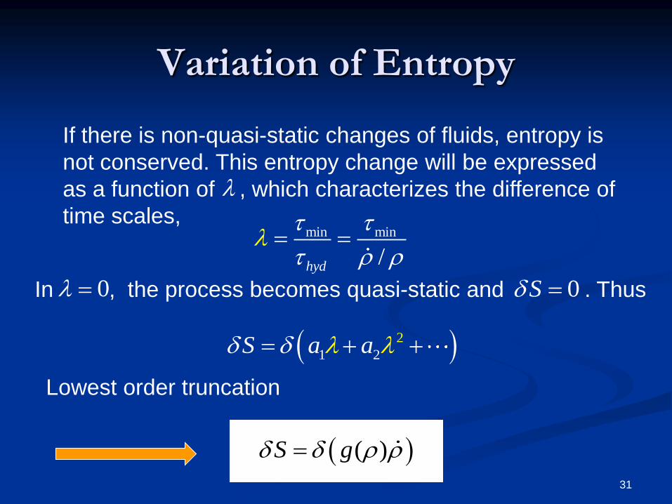
Variation of Entropy
( )S g
1
2
2S a a
min min
/hyd
If there is non-quasi-static changes of fluids, entropy is
not conserved. This entropy change will be expressed
as a function of , which characterizes the difference of
time scales,
Lowest order truncation
In , the process becomes quasi-static and . Thus0 0S
31
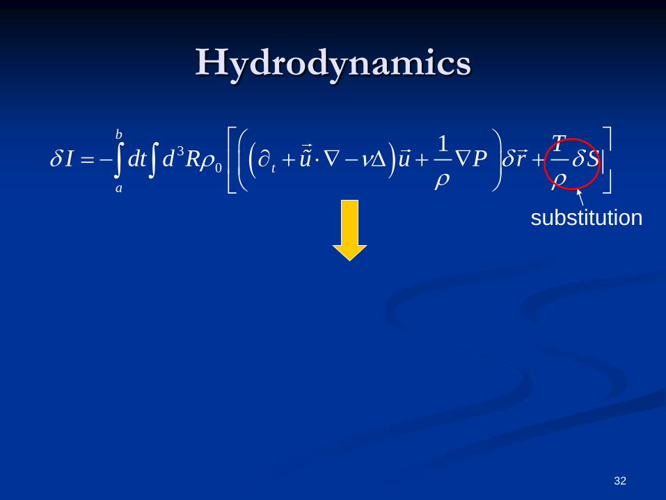
Hydrodynamics
3
0
1b
t
a
TI dt d R u u P r S
substitution
32
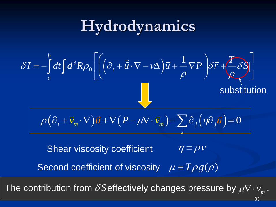
Hydrodynamics
3
0
1b
t
a
TI dt d R u u P r S
0t j j
j
m mv vu uP
Shear viscosity coefficient
Second coefficient of viscosity ( )T g
The contribution from effectively changes pressure by . Smv
substitution
33
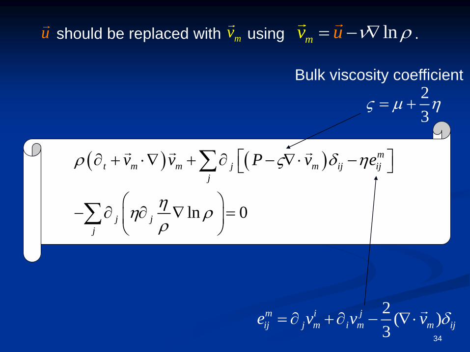
ln 0
m
t m m j m ij ij
j
j j
j
v v P v e
2
3
2( )
3
m i j
ij j m i m m ije v v v
should be replaced with using . u mv lnmv u
Bulk viscosity coefficient
34
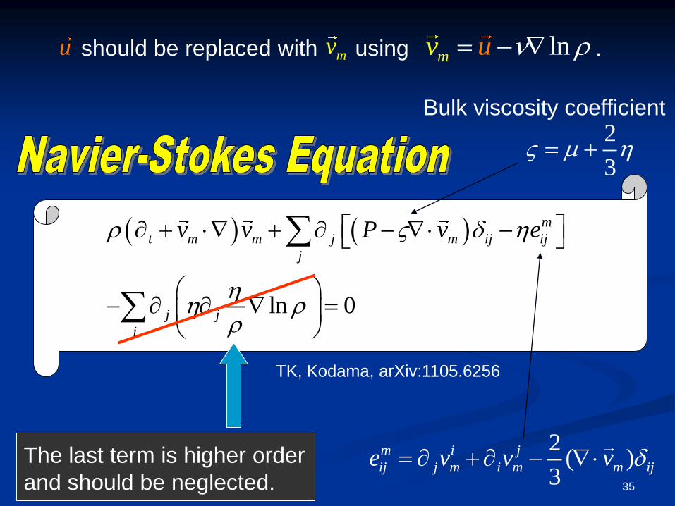
ln 0
m
t m m j m ij ij
j
j j
j
v v P v e
2
3
2( )
3
m i j
ij j m i m m ije v v v
should be replaced with using . u mv lnmv u
Bulk viscosity coefficient
The last term is higher order
and should be neglected.
TK, Kodama, arXiv:1105.6256
35
Results of SVM for NS
The most of viscous terms of NS is
obtained from the kinetic term as noise.
Differences of interaction among
constituent molecules of various fluids
affect only the form of the potential term.
The potential term changes only the
definition of pressure.
Thus NS is naturally obtained from
the framework of SVM !36
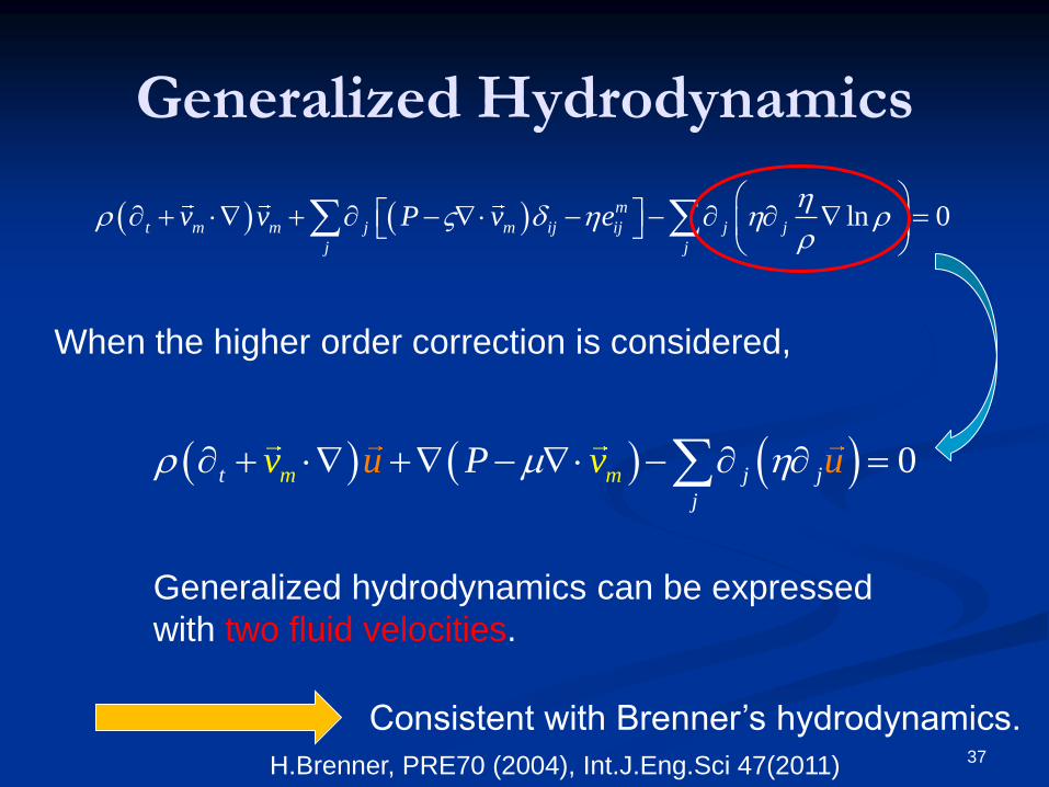
Generalized Hydrodynamics
ln 0m
t m m j m ij ij j j
j j
v v P v e
0t j j
j
m mv vu uP
When the higher order correction is considered,
Generalized hydrodynamics can be expressed
with two fluid velocities.
Consistent with Brenner‟s hydrodynamics.
H.Brenner, PRE70 (2004), Int.J.Eng.Sci 47(2011) 37
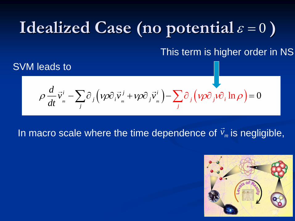
Idealized Case (no potential ) 0
SVM leads to
l 0nm m m
i j i
j i j j j i
jj
dv v v
dt
This term is higher order in NS
mvIn macro scale where the time dependence of is negligible,
38
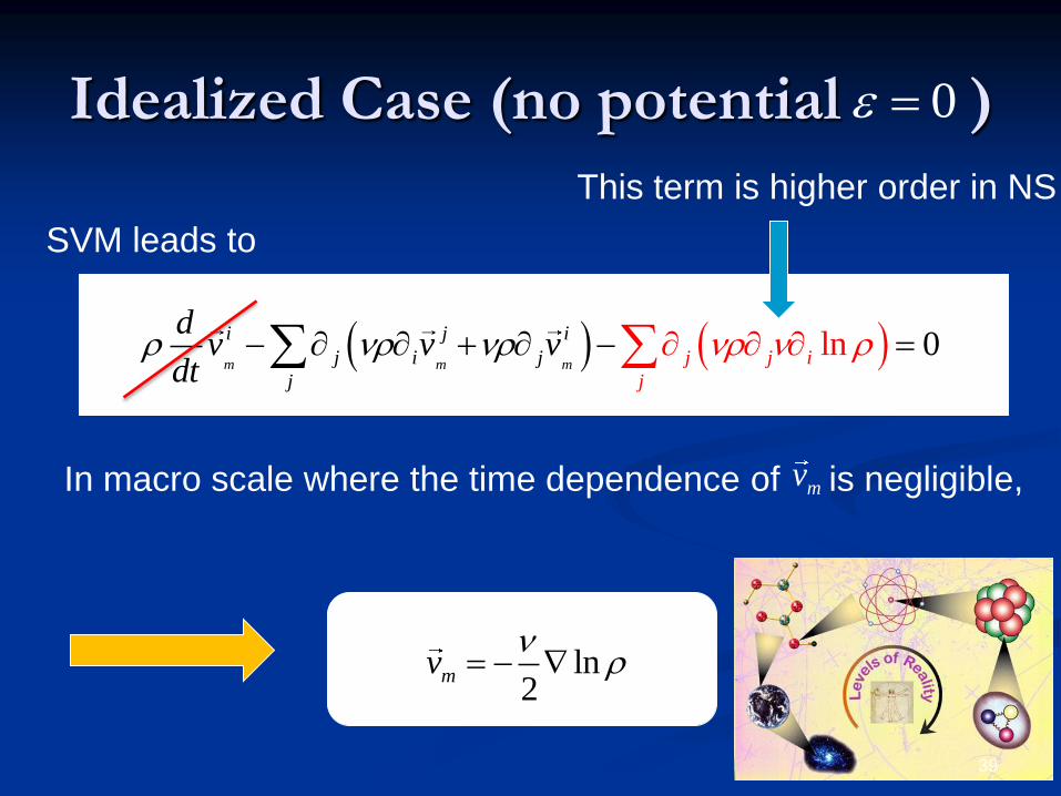
Idealized Case (no potential ) 0
SVM leads to
l 0nm m m
i j i
j i j j j i
jj
dv v v
dt
This term is higher order in NS
ln2
mv
mvIn macro scale where the time dependence of is negligible,
39
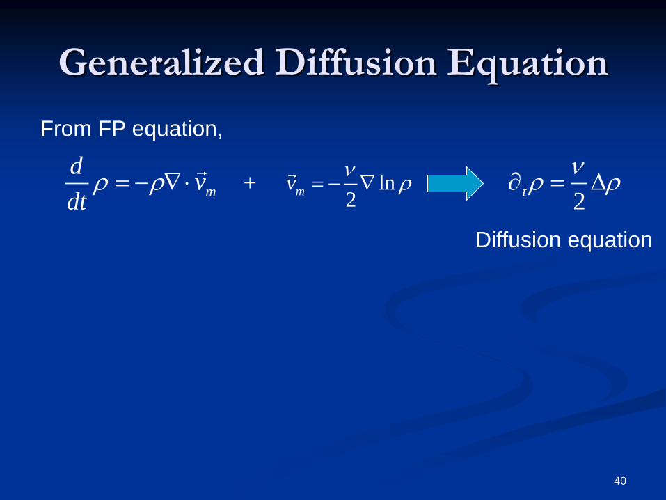
Generalized Diffusion Equation
m
dv
dt
From FP equation,
ln2
mv
Diffusion equation
2t
40
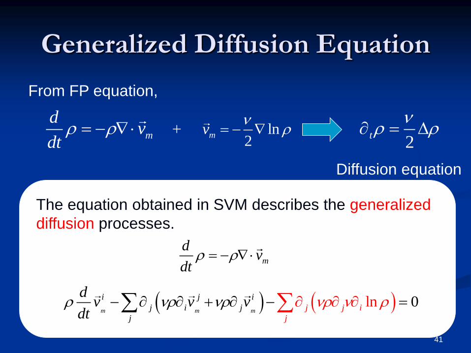
Generalized Diffusion Equation
m
dv
dt
From FP equation,
ln2
mv
Diffusion equation
2t
The equation obtained in SVM describes the generalized
diffusion processes.
m
dv
dt
l 0nm m m
i j i
j i j j j i
jj
dv v v
dt
41
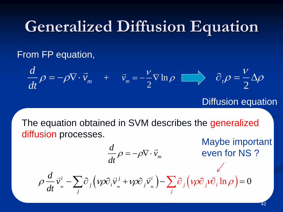
Generalized Diffusion Equation
m
dv
dt
From FP equation,
ln2
mv
Diffusion equation
2t
The equation obtained in SVM describes the generalized
diffusion processes.
m
dv
dt
l 0nm m m
i j i
j i j j j i
jj
dv v v
dt
Maybe important
even for NS ?
42
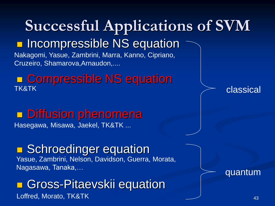
Successful Applications of SVM Incompressible NS equation
Compressible NS equation
Diffusion phenomena
Schroedinger equation
Gross-Pitaevskii equation
Nakagomi, Yasue, Zambrini, Marra, Kanno, Cipriano,
Cruzeiro, Shamarova,Arnaudon,....
Hasegawa, Misawa, Jaekel, TK&TK ...
Loffred, Morato, TK&TK
Yasue, Zambrini, Nelson, Davidson, Guerra, Morata,
Nagasawa, Tanaka,…
TK&TK classical
quantum
43
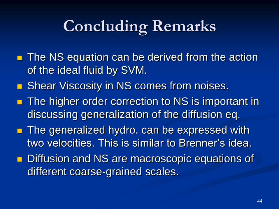
Concluding Remarks
The NS equation can be derived from the action
of the ideal fluid by SVM.
Shear Viscosity in NS comes from noises.
The higher order correction to NS is important in
discussing generalization of the diffusion eq.
The generalized hydro. can be expressed with
two velocities. This is similar to Brenner‟s idea.
Diffusion and NS are macroscopic equations of
different coarse-grained scales.
44
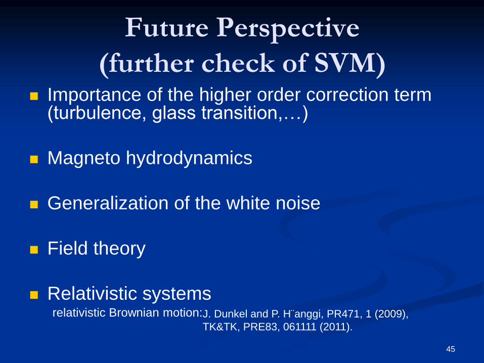
Future Perspective
(further check of SVM) Importance of the higher order correction term
(turbulence, glass transition,…)
Magneto hydrodynamics
Generalization of the white noise
Field theory
Relativistic systems
45
relativistic Brownian motion:J. Dunkel and P. H¨anggi, PR471, 1 (2009),
TK&TK, PRE83, 061111 (2011).

Future Perspective
(further check of SVM) Importance of the higher order correction term
(turbulence, glass transition,…)
Magneto hydrodynamics
Generalization of the white noise
Field theory
Relativistic systems
46
relativistic Brownian motion:J. Dunkel and P. H¨anggi, PR471, 1 (2009),
TK&TK, PRE83, 061111 (2011).
Danke Schön!
47
Ευχαριστώ!
Elena, Jörg,
Marcus, Igor
Danke Schön!
48
Ευχαριστώ!
Elena, Jörg,
Marcus, Igor
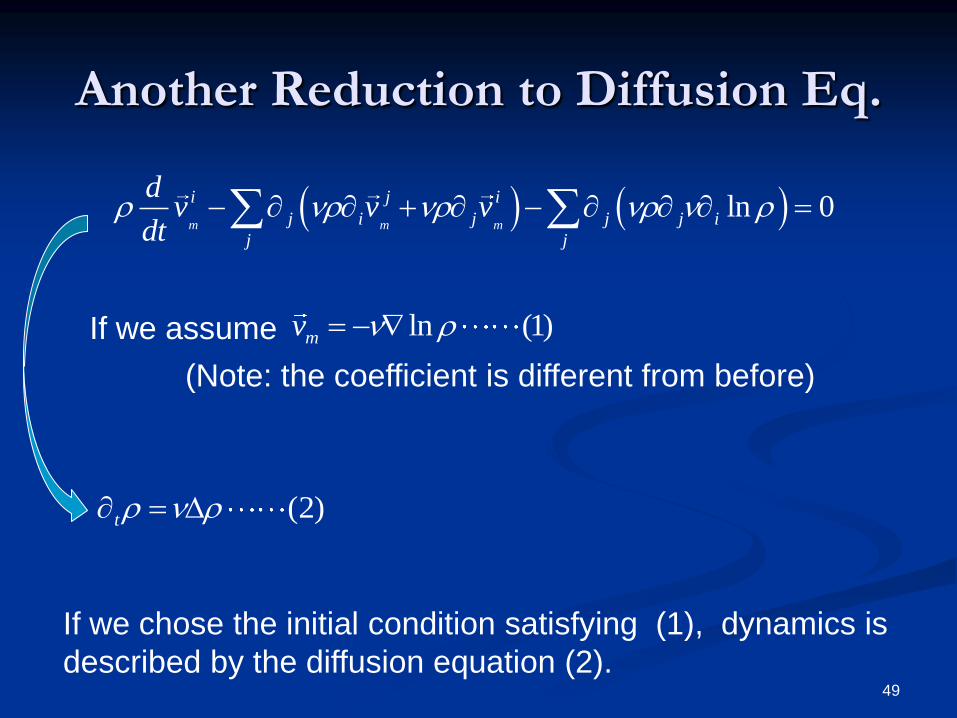
Another Reduction to Diffusion Eq.
ln 0m m m
i j i
j i j j j i
j j
dv v v
dt
If we assume ln (1)mv
(Note: the coefficient is different from before)
(2)t
If we chose the initial condition satisfying (1), dynamics is
described by the diffusion equation (2).49
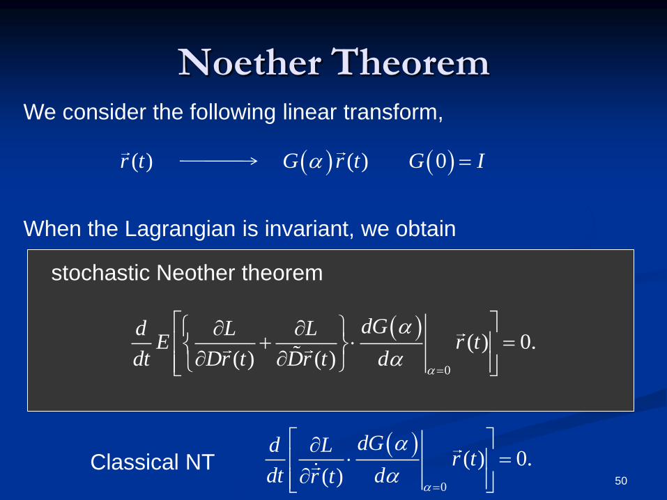
Noether Theorem
50
0
( ) 0.( ) ( )
dGd L LE r t
dt Dr t Dr t d
( )G r t( )r t 0G I
We consider the following linear transform,
When the Lagrangian is invariant, we obtain
stochastic Neother theorem
0
( ) 0.( )
dGd Lr t
dt dr t
Classical NT
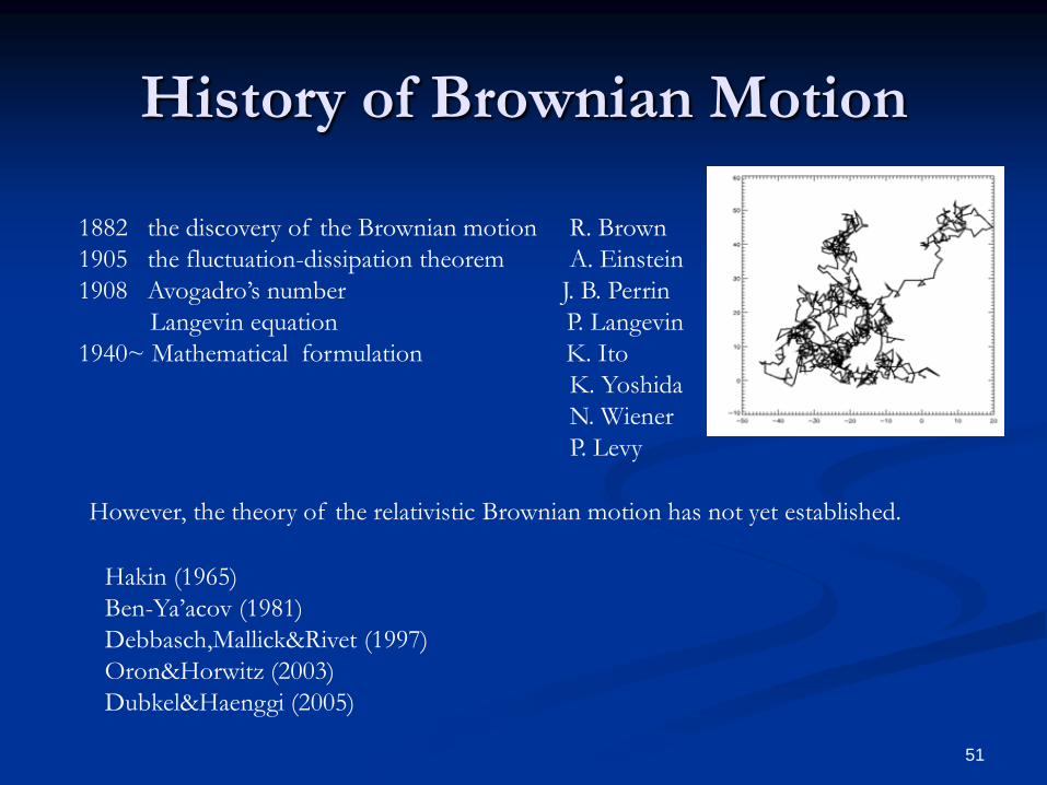
History of Brownian Motion
However, the theory of the relativistic Brownian motion has not yet established.
1882 the discovery of the Brownian motion R. Brown
1905 the fluctuation-dissipation theorem A. Einstein
1908 Avogadro’s number J. B. Perrin
Langevin equation P. Langevin
1940~ Mathematical formulation K. Ito
K. Yoshida
N. Wiener
P. Levy
Hakin (1965)
Ben-Ya’acov (1981)
Debbasch,Mallick&Rivet (1997)
Oron&Horwitz (2003)
Dubkel&Haenggi (2005)
51
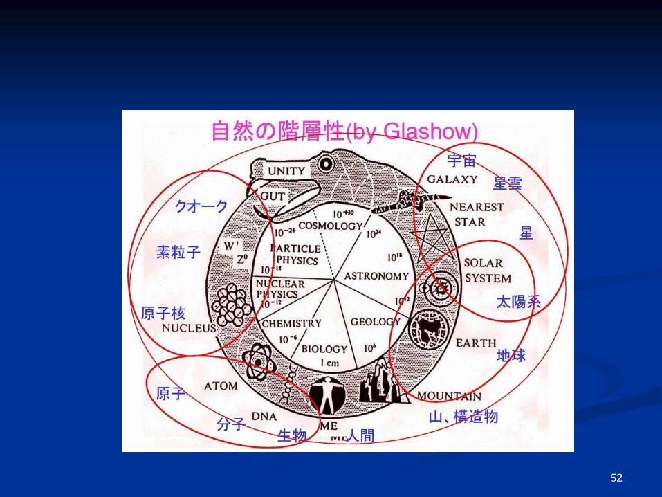
52

53
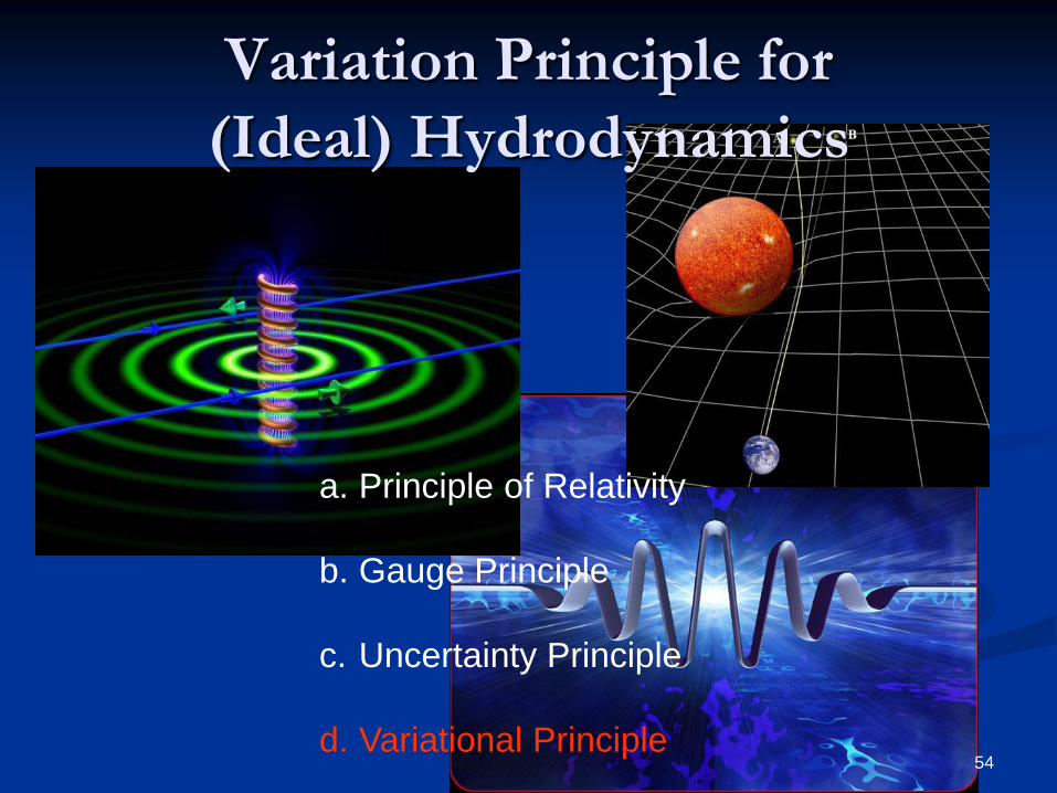
Variation Principle for
(Ideal) Hydrodynamics
a. Principle of Relativity
b. Gauge Principle
c. Uncertainty Principle
d. Variational Principle54