Stochastic Variational Inference - Columbia...
45
Journal of Machine Learning Research 14 (2013) 1303-1347 Submitted 6/12; Published 5/13 Stochastic Variational Inference Matthew D. Hoffman MATHOFFM@ADOBE. COM Adobe Research Adobe Systems Incorporated 601 Townsend Street San Francisco, CA 94103, USA David M. Blei BLEI @CS. PRINCETON. EDU Department of Computer Science Princeton University 35 Olden Street Princeton, NJ 08540, USA Chong Wang CHONGW@CS. CMU. EDU Machine Learning Department Carnegie Mellon University Gates Hillman Centers, 8110 5000 Forbes Avenue Pittsburgh, PA 15213, USA John Paisley JPAISLEY@BERKELEY. EDU Computer Science Division University of California Berkeley, CA 94720-1776, USA Editor: Tommi Jaakkola Abstract We develop stochastic variational inference, a scalable algorithm for approximating posterior dis- tributions. We develop this technique for a large class of probabilistic models and we demonstrate it with two probabilistic topic models, latent Dirichlet allocation and the hierarchical Dirichlet pro- cess topic model. Using stochastic variational inference, we analyze several large collections of documents: 300K articles from Nature, 1.8M articles from The New York Times, and 3.8M arti- cles from Wikipedia. Stochastic inference can easily handle data sets of this size and outperforms traditional variational inference, which can only handle a smaller subset. (We also show that the Bayesian nonparametric topic model outperforms its parametric counterpart.) Stochastic variational inference lets us apply complex Bayesian models to massive data sets. Keywords: Bayesian inference, variational inference, stochastic optimization, topic models, Bayesian nonparametrics 1. Introduction Modern data analysis requires computation with massive data. As examples, consider the following. (1) We have an archive of the raw text of two million books, scanned and stored online. We want to discover the themes in the texts, organize the books by subject, and build a navigator for users c 2013 Matthew D. Hoffman, David M. Blei, Chong Wang and John Paisley.
Transcript of Stochastic Variational Inference - Columbia...
Journal of Machine Learning Research 14 (2013) 1303-1347 Submitted 6/12; Published 5/13
Stochastic Variational Inference
Matthew D. Hoffman [email protected]
Adobe Research
Adobe Systems Incorporated
601 Townsend Street
San Francisco, CA 94103, USA
David M. Blei [email protected]
Department of Computer Science
Princeton University
35 Olden Street
Princeton, NJ 08540, USA
Chong Wang [email protected]
Machine Learning Department
Carnegie Mellon University
Gates Hillman Centers, 8110
5000 Forbes Avenue
Pittsburgh, PA 15213, USA
John Paisley [email protected]
Computer Science Division
University of California
Berkeley, CA 94720-1776, USA
Editor: Tommi Jaakkola
Abstract
We develop stochastic variational inference, a scalable algorithm for approximating posterior dis-
tributions. We develop this technique for a large class of probabilistic models and we demonstrate
it with two probabilistic topic models, latent Dirichlet allocation and the hierarchical Dirichlet pro-
cess topic model. Using stochastic variational inference, we analyze several large collections of
documents: 300K articles from Nature, 1.8M articles from The New York Times, and 3.8M arti-
cles from Wikipedia. Stochastic inference can easily handle data sets of this size and outperforms
traditional variational inference, which can only handle a smaller subset. (We also show that the
Bayesian nonparametric topic model outperforms its parametric counterpart.) Stochastic variational
inference lets us apply complex Bayesian models to massive data sets.
Keywords: Bayesian inference, variational inference, stochastic optimization, topic models, Bayesian
nonparametrics
1. Introduction
Modern data analysis requires computation with massive data. As examples, consider the following.
(1) We have an archive of the raw text of two million books, scanned and stored online. We want
to discover the themes in the texts, organize the books by subject, and build a navigator for users
c©2013 Matthew D. Hoffman, David M. Blei, Chong Wang and John Paisley.
HOFFMAN, BLEI, WANG AND PAISLEY
to explore our collection. (2) We have data from an online shopping website containing millions of
users’ purchase histories as well as descriptions of each item in the catalog. We want to recommend
items to users based on this information. (3) We are continuously collecting data from an online
feed of photographs. We want to build a classifier from these data. (4) We have measured the gene
sequences of millions of people. We want to make hypotheses about connections between observed
genes and other traits.
These problems illustrate some of the challenges to modern data analysis. Our data are com-
plex and high-dimensional; we have assumptions to make—from science, intuition, or other data
analyses—that involve structures we believe exist in the data but that we cannot directly observe;
and finally our data sets are large, possibly even arriving in a never-ending stream.
Statistical machine learning research has addressed some of these challenges by developing the
field of probabilistic modeling, a field that provides an elegant approach to developing new methods
for analyzing data (Pearl, 1988; Jordan, 1999; Bishop, 2006; Koller and Friedman, 2009; Murphy,
2012). In particular, probabilistic graphical models give us a visual language for expressing as-
sumptions about data and its hidden structure. The corresponding posterior inference algorithms
let us analyze data under those assumptions, inferring the hidden structure that best explains our
observations.
In descriptive tasks, like problems #1 and #4 above, graphical models help us explore the data—
the organization of books or the connections between genes and traits—with the hidden structure
probabilistically “filled in.” In predictive tasks, like problems #2 and #3, we use models to form
predictions about new observations. For example, we can make recommendations to users or pre-
dict the class labels of new images. With graphical models, we enjoy a powerful suite of probability
models to connect and combine; and we have general-purpose computational strategies for connect-
ing models to data and estimating the quantities needed to use them.
The problem we face is scale. Inference algorithms of the 1990s and 2000s used to be considered
scalable, but they cannot easily handle the amount of data that we described in the four examples
above. This is the problem we address here. We present an approach to computing with graphical
models that is appropriate for massive data sets, data that might not fit in memory or even be stored
locally. Our method does not require clusters of computers or specialized hardware, though it can
be further sped up with these amenities.
As an example of this approach to data analysis, consider topic models. Topic models are prob-
abilistic models of text used to uncover the hidden thematic structure in a collection of documents
(Blei, 2012). The main idea in a topic model is that there are a set of topics that describe the collec-
tion and each document exhibits those topics with different degrees. As a probabilistic model, the
topics and how they relate to the documents are hidden structure and the main computational prob-
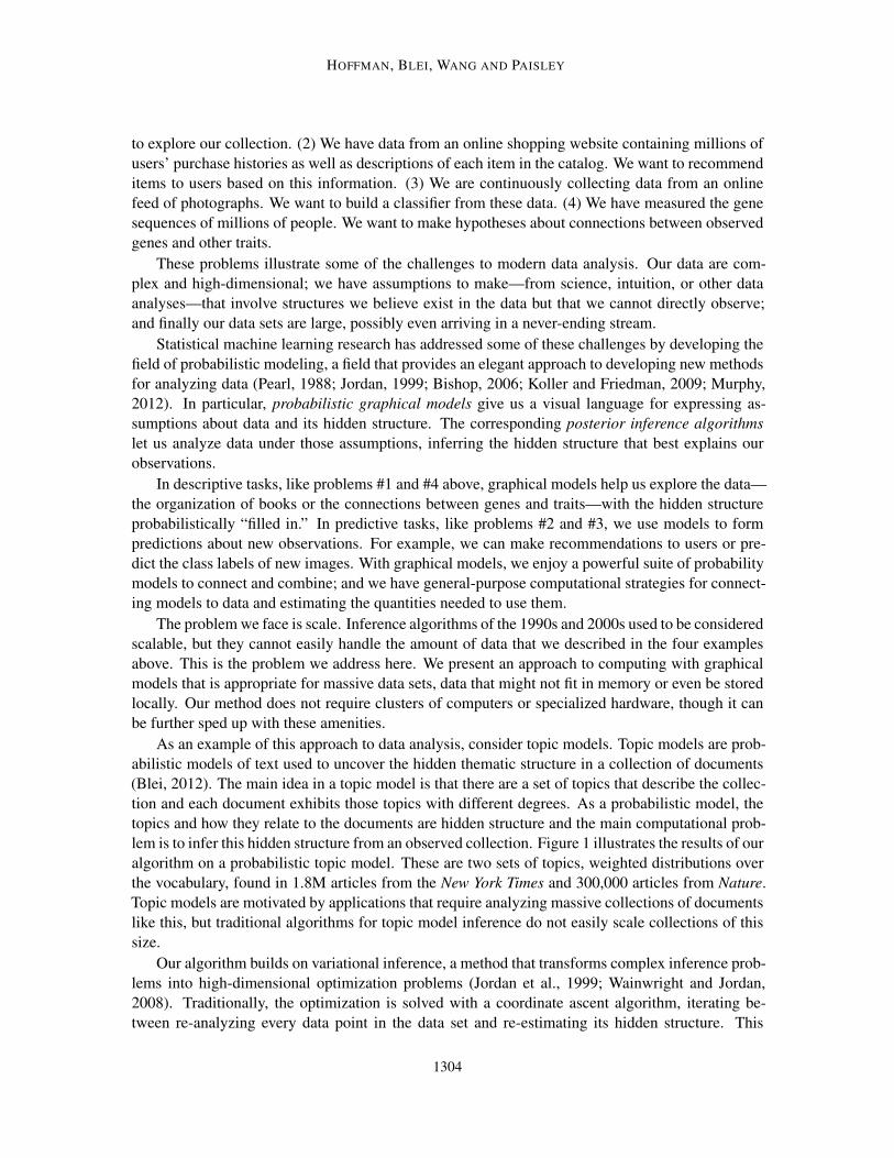
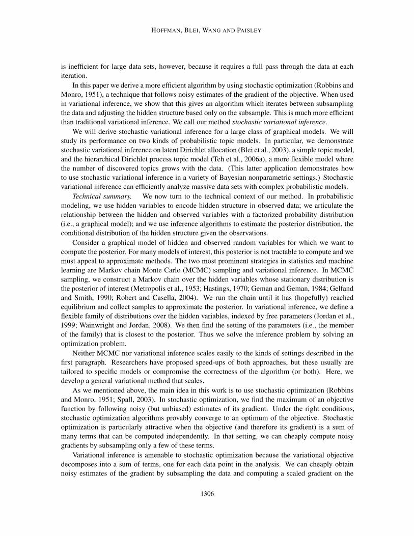
lem is to infer this hidden structure from an observed collection. Figure 1 illustrates the results of our
algorithm on a probabilistic topic model. These are two sets of topics, weighted distributions over
the vocabulary, found in 1.8M articles from the New York Times and 300,000 articles from Nature.
Topic models are motivated by applications that require analyzing massive collections of documents
like this, but traditional algorithms for topic model inference do not easily scale collections of this
size.
Our algorithm builds on variational inference, a method that transforms complex inference prob-
lems into high-dimensional optimization problems (Jordan et al., 1999; Wainwright and Jordan,
2008). Traditionally, the optimization is solved with a coordinate ascent algorithm, iterating be-
tween re-analyzing every data point in the data set and re-estimating its hidden structure. This
1304

STOCHASTIC VARIATIONAL INFERENCE
Figure 1: Posterior topics from the hierarchical Dirichlet process topic model on two large data sets.
These posteriors were approximated using stochastic variational inference with 1.8M ar-
ticles from the New York Times (top) and 350K articles from Nature (bottom). (See Sec-
tion 3.3 for the modeling details behind the hierarchical Dirichlet process and Section 4
for details about the empirical study.) Each topic is a weighted distribution over the vo-
cabulary and each topic’s plot illustrates its most frequent words.
1305
HOFFMAN, BLEI, WANG AND PAISLEY
is inefficient for large data sets, however, because it requires a full pass through the data at each
iteration.
In this paper we derive a more efficient algorithm by using stochastic optimization (Robbins and
Monro, 1951), a technique that follows noisy estimates of the gradient of the objective. When used
in variational inference, we show that this gives an algorithm which iterates between subsampling
the data and adjusting the hidden structure based only on the subsample. This is much more efficient
than traditional variational inference. We call our method stochastic variational inference.
We will derive stochastic variational inference for a large class of graphical models. We will
study its performance on two kinds of probabilistic topic models. In particular, we demonstrate
stochastic variational inference on latent Dirichlet allocation (Blei et al., 2003), a simple topic model,
and the hierarchical Dirichlet process topic model (Teh et al., 2006a), a more flexible model where
the number of discovered topics grows with the data. (This latter application demonstrates how
to use stochastic variational inference in a variety of Bayesian nonparametric settings.) Stochastic
variational inference can efficiently analyze massive data sets with complex probabilistic models.
Technical summary. We now turn to the technical context of our method. In probabilistic
modeling, we use hidden variables to encode hidden structure in observed data; we articulate the
relationship between the hidden and observed variables with a factorized probability distribution
(i.e., a graphical model); and we use inference algorithms to estimate the posterior distribution, the
conditional distribution of the hidden structure given the observations.
Consider a graphical model of hidden and observed random variables for which we want to
compute the posterior. For many models of interest, this posterior is not tractable to compute and we
must appeal to approximate methods. The two most prominent strategies in statistics and machine
learning are Markov chain Monte Carlo (MCMC) sampling and variational inference. In MCMC
sampling, we construct a Markov chain over the hidden variables whose stationary distribution is
the posterior of interest (Metropolis et al., 1953; Hastings, 1970; Geman and Geman, 1984; Gelfand
and Smith, 1990; Robert and Casella, 2004). We run the chain until it has (hopefully) reached
equilibrium and collect samples to approximate the posterior. In variational inference, we define a
flexible family of distributions over the hidden variables, indexed by free parameters (Jordan et al.,
1999; Wainwright and Jordan, 2008). We then find the setting of the parameters (i.e., the member
of the family) that is closest to the posterior. Thus we solve the inference problem by solving an
optimization problem.
Neither MCMC nor variational inference scales easily to the kinds of settings described in the
first paragraph. Researchers have proposed speed-ups of both approaches, but these usually are
tailored to specific models or compromise the correctness of the algorithm (or both). Here, we
develop a general variational method that scales.
As we mentioned above, the main idea in this work is to use stochastic optimization (Robbins
and Monro, 1951; Spall, 2003). In stochastic optimization, we find the maximum of an objective
function by following noisy (but unbiased) estimates of its gradient. Under the right conditions,
stochastic optimization algorithms provably converge to an optimum of the objective. Stochastic
optimization is particularly attractive when the objective (and therefore its gradient) is a sum of
many terms that can be computed independently. In that setting, we can cheaply compute noisy
gradients by subsampling only a few of these terms.
Variational inference is amenable to stochastic optimization because the variational objective
decomposes into a sum of terms, one for each data point in the analysis. We can cheaply obtain
noisy estimates of the gradient by subsampling the data and computing a scaled gradient on the
1306
STOCHASTIC VARIATIONAL INFERENCE
subsample. If we sample independently then the expectation of this noisy gradient is equal to
the true gradient. With one more detail—the idea of a natural gradient (Amari, 1998)—stochastic
variational inference has an attractive form:
1. Subsample one or more data points from the data.
2. Analyze the subsample using the current variational parameters.
3. Implement a closed-form update of the variational parameters.
4. Repeat.
While traditional algorithms require repeatedly analyzing the whole data set before updating the
variational parameters, this algorithm only requires that we analyze randomly sampled subsets. We
will show how to use this algorithm for a large class of graphical models.
Related work. Variational inference for probabilistic models was pioneered in the mid-1990s.
In Michael Jordan’s lab, the seminal papers of Saul et al. (1996); Saul and Jordan (1996) and
Jaakkola (1997) grew out of reading the statistical physics literature (Peterson and Anderson, 1987;
Parisi, 1988). In parallel, the mean-field methods explained in Neal and Hinton (1999) (originally
published in 1993) and Hinton and Van Camp (1993) led to variational algorithms for mixtures of
experts (Waterhouse et al., 1996).
In subsequent years, researchers began to understand the potential for variational inference in
more general settings and developed generic algorithms for conjugate exponential-family models
(Attias, 1999, 2000; Wiegerinck, 2000; Ghahramani and Beal, 2001; Xing et al., 2003). These
innovations led to automated variational inference, allowing a practitioner to write down a model
and immediately use variational inference to estimate its posterior (Bishop et al., 2003). For good
reviews of variational inference see Jordan et al. (1999) and Wainwright and Jordan (2008).
In this paper, we develop scalable methods for generic Bayesian inference by solving the vari-
ational inference problem with stochastic optimization (Robbins and Monro, 1951). Our algorithm
builds on the earlier approach of Sato (2001), whose algorithm only applies to the limited set of
models that can be fit with the EM algorithm (Dempster et al., 1977). Specifically, we generalize
his approach to the much wider set of probabilistic models that are amenable to closed-form coordi-
nate ascent inference. Further, in the sense that EM itself is a mean-field method (Neal and Hinton,
1999), our algorithm builds on the stochastic optimization approach to EM (Cappé and Moulines,
2009). Finally, we note that stochastic optimization was also used with variational inference in Platt
et al. (2008) for fast approximate inference in a specific model of web service activity.
For approximate inference, the main alternative to variational methods is Markov chain Monte
Carlo (MCMC) (Robert and Casella, 2004). Despite its popularity in Bayesian inference, relatively
little work has focused on developing MCMC algorithms that can scale to very large data sets. One
exception is sequential Monte Carlo, although these typically lack strong convergence guarantees
(Doucet et al., 2001). Another is the stochastic gradient Langevin method of Welling and Teh
(2011), which enjoys asymptotic convergence guarantees and also takes advantage of stochastic
optimization. Finally, in topic modeling, researchers have developed several approaches to parallel
MCMC (Newman et al., 2009; Smola and Narayanamurthy, 2010; Ahmed et al., 2012).
The organization of this paper. In Section 2, we review variational inference for graphical
models and then derive stochastic variational inference. In Section 3, we review probabilistic topic
models and Bayesian nonparametric models and then derive the stochastic variational inference
algorithms in these settings. In Section 4, we study stochastic variational inference on several large
text data sets.
1307

HOFFMAN, BLEI, WANG AND PAISLEY
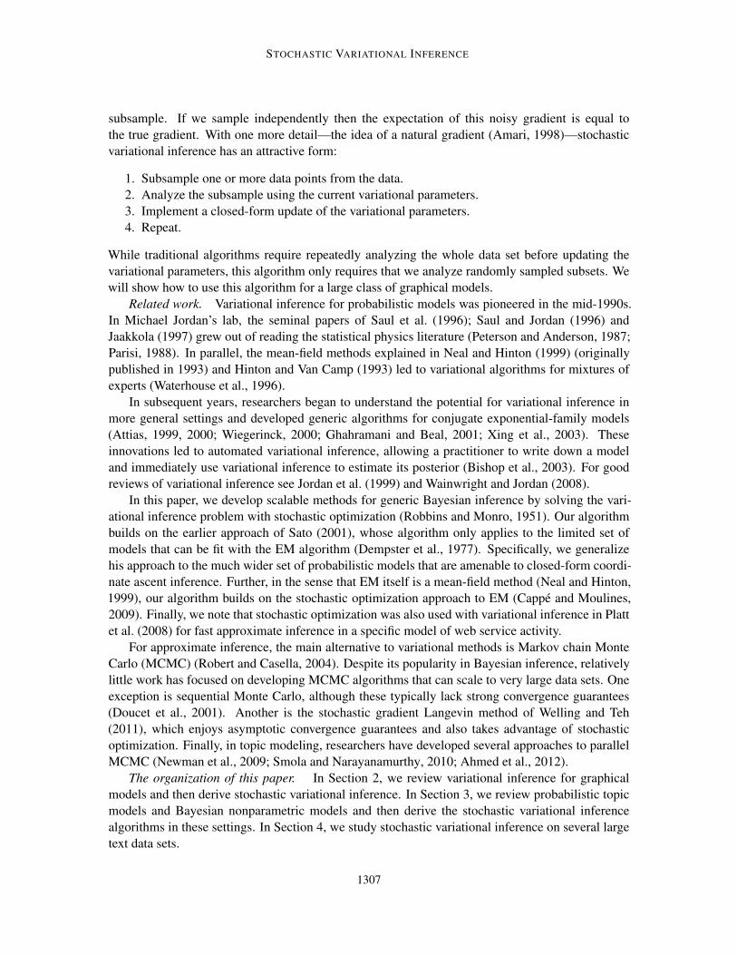
Figure 2: A graphical model with observations x1:N , local hidden variables z1:N and global hidden
variables β. The distribution of each observation xn only depends on its corresponding
local variable zn and the global variables β. (Though not pictured, each hidden variable zn,
observation xn, and global variable β may be a collection of multiple random variables.)
2. Stochastic Variational Inference
We derive stochastic variational inference, a stochastic optimization algorithm for mean-field vari-
ational inference. Our algorithm approximates the posterior distribution of a probabilistic model
with hidden variables, and can handle massive data sets of observations.
We divide this section into four parts.
1. We define the class of models to which our algorithm applies. We define local and global
hidden variables, and requirements on the conditional distributions within the model.
2. We review mean-field variational inference, an approximate inference strategy that seeks a
tractable distribution over the hidden variables which is close to the posterior distribution.
We derive the traditional variational inference algorithm for our class of models, which is a
coordinate ascent algorithm.
3. We review the natural gradient and derive the natural gradient of the variational objective
function. The natural gradient closely relates to coordinate ascent variational inference.
4. We review stochastic optimization, a technique that uses noisy estimates of a gradient to
optimize an objective function, and apply it to variational inference. Specifically, we use
stochastic optimization with noisy estimates of the natural gradient of the variational objective.
These estimates arise from repeatedly subsampling the data set. We show how the resulting
algorithm, stochastic variational inference, easily builds on traditional variational inference
algorithms but can handle much larger data sets.
2.1 Models with Local and Global Hidden Variables
Our class of models involves observations, global hidden variables, local hidden variables, and fixed
parameters. The N observations are x = x1:N ; the vector of global hidden variables is β; the N local
hidden variables are z = z1:N , each of which is a collection of J variables zn = zn,1:J; the vector of
fixed parameters is α. (Note we can easily allow α to partly govern any of the random variables,
1308

STOCHASTIC VARIATIONAL INFERENCE
such as fixed parts of the conditional distribution of observations. To keep notation simple, we
assume that they only govern the global hidden variables.)
The joint distribution factorizes into a global term and a product of local terms,
p(x,z,β |α) = p(β |α)N
∏n=1
p(xn,zn |β). (1)
Figure 2 illustrates the graphical model. Our goal is to approximate the posterior distribution of the
hidden variables given the observations, p(β,z |x).
The distinction between local and global hidden variables is determined by the conditional de-
pendencies. In particular, the nth observation xn and the nth local variable zn are conditionally
independent, given global variables β, of all other observations and local hidden variables,
p(xn,zn |x−n,z−n,β,α) = p(xn,zn |β,α).
The notation x−n and z−n refers to the set of variables except the nth.
This kind of model frequently arises in Bayesian statistics. The global variables β are parameters
endowed with a prior p(β) and each local variable zn contains the hidden structure that governs the
nth observation. For example, consider a Bayesian mixture of Gaussians. The global variables are
the mixture proportions and the means and variances of the mixture components; the local variable
zn is the hidden cluster label for the nth observation xn.
We have described the independence assumptions of the hidden variables. We make further
assumptions about the complete conditionals in the model. A complete conditional is the conditional
distribution of a hidden variable given the other hidden variables and the observations. We assume
that these distributions are in the exponential family,
p(β |x,z,α) = h(β)exp{ηg(x,z,α)⊤t(β)−ag(ηg(x,z,α))}, (2)
p(zn j |xn,zn,− j,β) = h(zn j)exp{ηℓ(xn,zn,− j,β)⊤t(zn j)−aℓ(ηℓ(xn,zn,− j,β))}. (3)
The scalar functions h(·) and a(·) are respectively the base measure and log-normalizer; the vector
functions η(·) and t(·) are respectively the natural parameter and sufficient statistics.1 These are
conditional distributions, so the natural parameter is a function of the variables that are being con-
ditioned on. (The subscripts on the natural parameter η indicate complete conditionals for local or
global variables.) For the local variables zn j, the complete conditional distribution is determined by
the global variables β and the other local variables in the nth context, that is, the nth data point xn
and the local variables zn,− j. This follows from the factorization in Equation 1.
These assumptions on the complete conditionals imply a conjugacy relationship between the
global variables β and the local contexts (zn,xn), and this relationship implies a specific form of
the complete conditional for β. Specifically, the distribution of the local context given the global
variables must be in an exponential family,
p(xn,zn|β) = h(xn,zn)exp{β⊤t(xn,zn)−aℓ(β)}. (4)
1. We use overloaded notation for the functions h(·) and t(·) so that they depend on the names of their arguments; for
example, h(zn j) can be thought of as a shorthand for the more formal (but more cluttered) notation hzn j(zn j). This is
analogous to the standard convention of overloading the probability function p(·).
1309

HOFFMAN, BLEI, WANG AND PAISLEY
The prior distribution p(β) must also be in an exponential family,
p(β) = h(β)exp{α⊤t(β)−ag(α)}. (5)
The sufficient statistics are t(β) = (β,−aℓ(β)) and thus the hyperparameter α has two components
α = (α1,α2). The first component α1 is a vector of the same dimension as β; the second component
α2 is a scalar.
Equations 4 and 5 imply that the complete conditional for the global variable in Equation 2 is in
the same exponential family as the prior with natural parameter
ηg(x,z,α) = (α1 +∑Nn=1 t(zn,xn),α2 +N). (6)
This form will be important when we derive stochastic variational inference in Section 2.4. See
Bernardo and Smith (1994) for a general discussion of conjugacy and the exponential family.
This family of distributions—those with local and global variables, and where the complete
conditionals are in the exponential family—contains many useful statistical models from the ma-
chine learning and statistics literature. Examples include Bayesian mixture models (Ghahramani
and Beal, 2000; Attias, 2000), latent Dirichlet allocation (Blei et al., 2003), hidden Markov models
(and many variants) (Rabiner, 1989; Fine et al., 1998; Fox et al., 2011b; Paisley and Carin, 2009),
Kalman filters (and many variants) (Kalman, 1960; Fox et al., 2011a), factorial models (Ghahramani
and Jordan, 1997), hierarchical linear regression models (Gelman and Hill, 2007), hierarchical pro-
bit classification models (McCullagh and Nelder, 1989; Girolami and Rogers, 2006), probabilistic
factor analysis/matrix factorization models (Spearman, 1904; Tipping and Bishop, 1999; Collins
et al., 2002; Wang, 2006; Salakhutdinov and Mnih, 2008; Paisley and Carin, 2009; Hoffman et al.,
2010b), certain Bayesian nonparametric mixture models (Antoniak, 1974; Escobar and West, 1995;
Teh et al., 2006a), and others.2
Analyzing data with one of these models amounts to computing the posterior distribution of the
hidden variables given the observations,
p(z,β |x) =p(x,z,β)∫
p(x,z,β)dzdβ. (7)
We then use this posterior to explore the hidden structure of our data or to make predictions about
future data. For many models however, such as the examples listed above, the denominator in
Equation 7 is intractable to compute. Thus we resort to approximate posterior inference, a problem
that has been a focus of modern Bayesian statistics. We now turn to mean-field variational inference,
the approximation inference technique which roots our strategy for scalable inference.
2.2 Mean-Field Variational Inference
Variational inference casts the inference problem as an optimization. We introduce a family of dis-
tributions over the hidden variables that is indexed by a set of free parameters, and then optimize
those parameters to find the member of the family that is closest to the posterior of interest. (Close-
ness is measured with Kullback-Leibler divergence.) We use the resulting distribution, called the
variational distribution, to approximate the posterior.
2. We note that our assumptions can be relaxed to the case where the full conditional p(β|x,z) is not tractable, but each
partial conditional p(βk|x,z,β−k) associated with the global variable βk is in a tractable exponential family. The topic
models of the next section do not require this complexity, so we chose to keep the derivation a little simpler.
1310
STOCHASTIC VARIATIONAL INFERENCE
In this section we review mean-field variational inference, the form of variational inference that
uses a family where each hidden variable is independent. We describe the variational objective func-
tion, discuss the mean-field variational family, and derive the traditional coordinate ascent algorithm
for fitting the variational parameters. This algorithm is a stepping stone to stochastic variational in-
ference.
The evidence lower bound. Variational inference minimizes the Kullback-Leibler (KL) di-
vergence from the variational distribution to the posterior distribution. It maximizes the evidence
lower bound (ELBO), a lower bound on the logarithm of the marginal probability of the observa-
tions log p(x). The ELBO is equal to the negative KL divergence up to an additive constant.
We derive the ELBO by introducing a distribution over the hidden variables q(z,β) and using
Jensen’s inequality. (Jensen’s inequality and the concavity of the logarithm function imply that
logE[ f (y)] ≥ E[log f (y)] for any random variable y.) This gives the following bound on the log
marginal,
log p(x) = log
∫p(x,z,β)dzdβ
= log
∫p(x,z,β)
q(z,β)
q(z,β)dzdβ
= log
(
Eq
[
p(x,z,β)
q(z,β)
])
≥ Eq[log p(x,z,β)]−Eq[logq(z,β)] (8)
, L(q).
The ELBO contains two terms. The first term is the expected log joint, Eq[log p(x,z,β)]. The second
term is the entropy of the variational distribution, −Eq[logq(z,β)]. Both of these terms depend on
q(z,β), the variational distribution of the hidden variables.
We restrict q(z,β) to be in a family that is tractable, one for which the expectations in the ELBO
can be efficiently computed. We then try to find the member of the family that maximizes the ELBO.
Finally, we use the optimized distribution as a proxy for the posterior.
Solving this maximization problem is equivalent to finding the member of the family that is
closest in KL divergence to the posterior (Jordan et al., 1999; Wainwright and Jordan, 2008),
KL(q(z,β)||p(z,β|x)) = Eq [logq(z,β)]−Eq [log p(z,β |x)]
= Eq [logq(z,β)]−Eq [log p(x,z,β)]+ log p(x)
= −L(q)+ const.
log p(x) is replaced by a constant because it does not depend on q.
The mean-field variational family. The simplest variational family of distributions is the mean-
field family. In this family, each hidden variable is independent and governed by its own parameter,
q(z,β) = q(β |λ)N
∏n=1
J
∏j=1
q(zn j |φn j). (9)
The global parameters λ govern the global variables; the local parameters φn govern the local vari-
ables in the nth context. The ELBO is a function of these parameters.
1311
HOFFMAN, BLEI, WANG AND PAISLEY
Equation 9 gives the factorization of the variational family, but does not specify its form. We set
q(β|λ) and q(zn j|φn j) to be in the same exponential family as the complete conditional distributions
p(β|x,z) and p(zn j|xn,zn,− j,β), from Equations 2 and 3. The variational parameters λ and φn j are
the natural parameters to those families,
q(β |λ) = h(β)exp{λ⊤t(β)−ag(λ)}, (10)
q(zn j |φn j) = h(zn j)exp{φ⊤n jt(zn j)−aℓ(φn j)}. (11)
These forms of the variational distributions lead to an easy coordinate ascent algorithm. Further, the
optimal mean-field distribution, without regard to its particular functional form, has factors in these
families (Bishop, 2006).
Note that assuming that these exponential families are the same as their corresponding condi-
tionals means that t(·) and h(·) in Equation 10 are the same functions as t(·) and h(·) in Equation 2.
Likewise, t(·) and h(·) in Equation 11 are the same as in Equation 3. We will sometimes suppress
the explicit dependence on φ and λ, substituting q(zn j) for q(zn j|φn j) and q(β) for q(β|λ).
The mean-field family has several computational advantages. For one, the entropy term decom-
poses,
−Eq[logq(z,β)] =−Eλ[logq(β)]−N
∑n=1
J
∑j=1
Eφn j[logq(zn j)],
where Eφn j[·] denotes an expectation with respect to q(zn j |φn j) and Eλ[·] denotes an expectation
with respect to q(β |λ). Its other computational advantages will emerge as we derive the gradients
of the variational objective and the coordinate ascent algorithm.
The gradient of the ELBO and coordinate ascent inference. We have defined the objective
function in Equation 8 and the variational family in Equations 9, 10 and 11. Our goal is to optimize
the objective with respect to the variational parameters.
In traditional mean-field variational inference, we optimize Equation 8 with coordinate ascent.
We iteratively optimize each variational parameter, holding the other parameters fixed. With the
assumptions that we have made about the model and variational distribution—that each conditional
is in an exponential family and that the corresponding variational distribution is in the same expo-
nential family—we can optimize each coordinate in closed form.
We first derive the coordinate update for the parameter λ to the variational distribution of the
global variables q(β |λ). As a function of λ, we can rewrite the objective as
L(λ) = Eq[log p(β |x,z)]−Eq[logq(β)]+ const. (12)
The first two terms are expectations that involve β; the third term is constant with respect to λ. The
constant absorbs quantities that depend only on the other hidden variables. Those quantities do not
depend on q(β |λ) because all variables are independent in the mean-field family.
Equation 12 reproduces the full ELBO in Equation 8. The second term of Equation 12 is the
entropy of the global variational distribution. The first term derives from the expected log joint
likelihood, where we use the chain rule to separate terms that depend on the variable β from terms
that do not,
Eq[log p(x,z,β)] = Eq[log p(x,z)]+Eq[log p(β |x,z)].
The constant absorbs Eq[log p(x,z)], leaving the expected log conditional Eq[log p(β |x,z)].
1312

STOCHASTIC VARIATIONAL INFERENCE
Finally, we substitute the form of q(β |λ) in Equation 10 to obtain the final expression for the
ELBO as a function of λ,
L(λ) = Eq[ηg(x,z,α)]⊤∇λag(λ)−λ⊤∇λag(λ)+ag(λ)+ const. (13)
In the first and second terms on the right side, we used the exponential family identity that the expec-
tation of the sufficient statistics is the gradient of the log normalizer, Eq[t(β)] = ∇λag(λ). The con-
stant has further absorbed the expected log normalizer of the conditional distribution
−Eq[ag(ηg(x,z,α))], which does not depend on q(β).
Equation 13 simplifies the ELBO as a function of the global variational parameter. To derive
the coordinate ascent update, we take the gradient,
∇λL = ∇2λag(λ)(Eq[ηg(x,z,α)]−λ). (14)
We can set this gradient to zero by setting
λ = Eq[ηg(x,z,α)]. (15)
This sets the global variational parameter equal to the expected natural parameter of its complete
conditional distribution. Implementing this update, holding all other variational parameters fixed,
optimizes the ELBO over λ. Notice that the mean-field assumption plays an important role. The
update is the expected conditional parameter Eq[ηg(x,z,α)], which is an expectation of a function of
the other random variables and observations. Thanks to the mean-field assumption, this expectation
is only a function of the local variational parameters and does not depend on λ.
We now turn to the local parameters φn j. The gradient is nearly identical to the global case,
∇φn jL = ∇2
φn jaℓ(φn j)(Eq[ηℓ(xn,zn,− j,β)]−φn j).
It equals zero when
φn j = Eq[ηℓ(xn,zn,− j,β)]. (16)
Mirroring the global update, this expectation does not depend on φn j. However, while the global
update in Equation 15 depends on all the local variational parameters—and note there is a set of
local parameters for each of the N observations—the local update in Equation 16 only depends
on the global parameters and the other parameters associated with the nth context. The computa-
tional difference between local and global updates will be important in the scalable algorithm of
Section 2.4.
The updates in Equations 15 and 16 form the algorithm for coordinate ascent variational infer-
ence, iterating between updating each local parameter and the global parameters. The full algorithm
is in Figure 3, which is guaranteed to find a local optimum of the ELBO. Computing the expecta-
tions at each step is easy for directed graphical models with tractable complete conditionals, and in
Section 3 we show that these updates are tractable for many topic models. Figure 3 is the “classical”
variational inference algorithm, used in many settings.
As an aside, these updates reveal a connection between mean-field variational inference and
Gibbs sampling (Gelfand and Smith, 1990). In Gibbs sampling, we iteratively sample from each
complete conditional. In variational inference, we take variational expectations of the natural param-
eters of the same distributions. The updates also show a connection to the expectation-maximization
1313

HOFFMAN, BLEI, WANG AND PAISLEY
1: Initialize λ(0) randomly.
2: repeat
3: for each local variational parameter φn j do
4: Update φn j, φ(t)n j = Eq(t−1) [ηℓ, j(xn,zn,− j,β)].
5: end for
6: Update the global variational parameters, λ(t) = Eq(t) [ηg(z1:N ,x1:N)].7: until the ELBO converges
Figure 3: Coordinate ascent mean-field variational inference.
(EM) algorithm (Dempster et al., 1977)—Equation 16 corresponds to the E step, and Equation 15
corresponds to the M step (Neal and Hinton, 1999).
We mentioned that the local steps (Steps 3 and 4 in Figure 3) only require computation with
the global parameters and the nth local context. Thus, the data can be distributed across many
machines and the local variational updates can be implemented in parallel. These results can then
be aggregated in Step 6 to find the new global variational parameters.
However, the local steps also reveal an inefficiency in the algorithm. The algorithm begins by
initializing the global parameters λ randomly—the initial value of λ does not reflect any regularity
in the data. But before completing even one iteration, the algorithm must analyze every data point
using these initial (random) values. This is wasteful, especially if we expect that we can learn
something about the global variational parameters from only a subset of the data.
We solve this problem with stochastic optimization. This leads to stochastic variational infer-
ence, an efficient algorithm that continually improves its estimate of the global parameters as it
analyzes more observations. Though the derivation requires some details, we have now described
all of the computational components of the algorithm. (See Figure 4.) At each iteration, we sam-
ple a data point from the data set and compute its optimal local variational parameters; we form
intermediate global parameters using classical coordinate ascent updates where the sampled data
point is repeated N times; finally, we set the new global parameters to a weighted average of the old
estimate and the intermediate parameters.
The algorithm is efficient because it need not analyze the whole data set before improving the
global variational parameters, and the per-iteration steps only require computation about a single lo-
cal context. Furthermore, it only uses calculations from classical coordinate inference. Any existing
implementation of variational inference can be easily configured to this scalable alternative.
We now show how stochastic inference arises by applying stochastic optimization to the natural
gradients of the variational objective. We first discuss natural gradients and their relationship to the
coordinate updates in mean-field variational inference.
2.3 The Natural Gradient of the ELBO
The natural gradient of a function accounts for the information geometry of its parameter space,
using a Riemannian metric to adjust the direction of the traditional gradient. Amari (1998) discusses
natural gradients for maximum-likelihood estimation, which give faster convergence than standard
1314
STOCHASTIC VARIATIONAL INFERENCE
gradients. In this section we describe Riemannian metrics for probability distributions and the
natural gradient of the ELBO.
Gradients and probability distributions. The classical gradient method for maximization tries
to find a maximum of a function f (λ) by taking steps of size ρ in the direction of the gradient,
λ(t+1) = λ(t)+ρ∇λ f (λ(t)).
The gradient (when it exists) points in the direction of steepest ascent. That is, the gradient ∇λ f (λ)points in the same direction as the solution to
argmaxdλ
f (λ+dλ) subject to ||dλ||2 < ε2 (17)
for sufficiently small ε. Equation 17 implies that if we could only move a tiny distance ε away
from λ then we should move in the direction of the gradient. Initially this seems reasonable, but
there is a complication. The gradient direction implicitly depends on the Euclidean distance metric
associated with the space in which λ lives. However, the Euclidean metric might not capture a
meaningful notion of distance between settings of λ.
The problem with Euclidean distance is especially clear in our setting, where we are trying
to optimize an objective with respect to a parameterized probability distribution q(β |λ). When
optimizing over a probability distribution, the Euclidean distance between two parameter vectors
λ and λ′ is often a poor measure of the dissimilarity of the distributions q(β |λ) and q(β |λ′). For
example, suppose q(β) is a univariate normal and λ is the mean µ and scale σ. The distributions
N (0,10000) and N (10,10000) are almost indistinguishable, and the Euclidean distance between
their parameter vectors is 10. In contrast, the distributions N (0,0.01) and N (0.1,0.01) barely
overlap, but this is not reflected in the Euclidean distance between their parameter vectors, which
is only 0.1. The natural gradient corrects for this issue by redefining the basic definition of the
gradient (Amari, 1998).
Natural gradients and probability distributions. A natural measure of dissimilarity between
probability distributions is the symmetrized KL divergence
DsymKL (λ,λ′) = Eλ
[
logq(β |λ)q(β |λ′)
]
+Eλ′
[
logq(β |λ′)q(β |λ)
]
. (18)
Symmetrized KL depends on the distributions themselves, rather than on how they are parameter-
ized; it is invariant to parameter transformations.
With distances defined using symmetrized KL, we find the direction of steepest ascent in the
same way as for gradient methods,
argmaxdλ
f (λ+dλ) subject to DsymKL (λ,λ+dλ)< ε. (19)
As ε→ 0, the solution to this problem points in the same direction as the natural gradient. While the
Euclidean gradient points in the direction of steepest ascent in Euclidean space, the natural gradient
points in the direction of steepest ascent in the Riemannian space, that is, the space where local
distance is defined by KL divergence rather than the L2 norm.
We manage the more complicated constraint in Equation 19 with a Riemannian metric G(λ)(Do Carmo, 1992). This metric defines linear transformations of λ under which the squared Eu-
clidean distance between λ and a nearby vector λ+dλ is the KL between q(β|λ) and q(β|λ+dλ),
dλT G(λ)dλ = DsymKL (λ,λ+dλ), (20)
1315

HOFFMAN, BLEI, WANG AND PAISLEY
and note that the transformation can be a function of λ. Amari (1998) showed that we can compute
the natural gradient by premultiplying the gradient by the inverse of the Riemannian metric G(λ)−1,
∇λ f (λ), G(λ)−1∇λ f (λ),
where G is the Fisher information matrix of q(λ) (Amari, 1982; Kullback and Leibler, 1951),
G(λ) = Eλ
[
(∇λ logq(β |λ))(∇λ logq(β |λ))⊤]
. (21)
We can show that Equation 21 satisfies Equation 20 by approximating logq(β |λ+ dλ) using the
first-order Taylor approximations about λ
logq(β|λ+dλ) = O(dλ2)+ logq(β|λ)+dλ⊤∇λ logq(β|λ),
q(β|λ+dλ) = O(dλ2)+q(β|λ)+q(β|λ)dλ⊤∇λ logq(β|λ),
and plugging the result into Equation 18:
DsymKL (λ,λ+dλ) =
∫β(q(β|λ+dλ)−q(β|λ))(logq(β|λ+dλ)− logq(β|λ))dβ
= O(dλ3)+∫
βq(β|λ)(dλ⊤∇λ logq(β|λ))2dβ
= O(dλ3)+Eq[(dλ⊤∇λ logq(β|λ))2] = O(dλ3)+dλ⊤G(λ)dλ.
For small enough dλ we can ignore the O(dλ3) term.
When q(β |λ) is in the exponential family (Equation 10) the metric is the second derivative of
the log normalizer,
G(λ) = Eλ
[
(∇λ log p(β |λ))(∇λ log p(β |λ))⊤]
= Eλ
[
(t(β)−Eλ[t(β)])(t(β)−Eλ[t(β)])⊤]
= ∇2λag(λ).
This follows from the exponential family identity that the Hessian of the log normalizer function a
with respect to the natural parameter λ is the covariance matrix of the sufficient statistic vector t(β).Natural gradients and mean field variational inference. We now return to variational in-
ference and compute the natural gradient of the ELBO with respect to the variational parameters.
Researchers have used the natural gradient in variational inference for nonlinear state space models
(Honkela et al., 2008) and Bayesian mixtures (Sato, 2001).3
Consider the global variational parameter λ. The gradient of the ELBO with respect to λ is
in Equation 14. Since λ is a natural parameter to an exponential family distribution, the Fisher
metric defined by q(β) is ∇2λag(λ). Note that the Fisher metric is the first term in Equation 14. We
premultiply the gradient by the inverse Fisher information to find the natural gradient. This reveals
that the natural gradient has the following simple form,
∇λL = Eφ[ηg(x,z,α)]−λ. (22)
3. Our work here—using the natural gradient in a stochastic optimization algorithm—is closest to that of Sato (2001),
though we develop the algorithm via a different path and Sato does not address models for which the joint conditional
p(zn|β,xn) is not tractable.
1316
STOCHASTIC VARIATIONAL INFERENCE
An analogous computation goes through for the local variational parameters,
∇φn jL = Eλ,φn,− j
[ηℓ(xn,zn,− j,β)]−φn j.
The natural gradients are closely related to the coordinate ascent updates of Equation 15 or Equa-
tion 16. Consider a full set of variational parameters λ and φ. We can compute the natural gradient
by computing the coordinate updates in parallel and subtracting the current setting of the parameters.
The classical coordinate ascent algorithm can thus be interpreted as a projected natural gradient al-
gorithm (Sato, 2001). Updating a parameter by taking a natural gradient step of length one is
equivalent to performing a coordinate update.
We motivated natural gradients by mathematical reasoning around the geometry of the parame-
ter space. More importantly, however, natural gradients are easier to compute than classical gradi-
ents. They are easier to compute because premultiplying by the Fisher information matrix—which
we must do to compute the classical gradient in Equation 14 but which disappears from the natural
gradient in Equation 22—is prohibitively expensive for variational parameters with many compo-
nents. In the next section we will see that efficiently computing the natural gradient lets us develop
scalable variational inference algorithms.
2.4 Stochastic Variational Inference
The coordinate ascent algorithm in Figure 3 is inefficient for large data sets because we must opti-
mize the local variational parameters for each data point before re-estimating the global variational
parameters. Stochastic variational inference uses stochastic optimization to fit the global variational
parameters. We repeatedly subsample the data to form noisy estimates of the natural gradient of the
ELBO, and we follow these estimates with a decreasing step-size.
We have reviewed mean-field variational inference in models with exponential family condition-
als and showed that the natural gradient of the variational objective function is easy to compute. We
now discuss stochastic optimization, which uses a series of noisy estimates of the gradient, and use
it with noisy natural gradients to derive stochastic variational inference.
Stochastic optimization. Stochastic optimization algorithms follow noisy estimates of the
gradient with a decreasing step size. Noisy estimates of a gradient are often cheaper to compute
than the true gradient, and following such estimates can allow algorithms to escape shallow local
optima of complex objective functions. In statistical estimation problems, including variational
inference of the global parameters, the gradient can be written as a sum of terms (one for each
data point) and we can compute a fast noisy approximation by subsampling the data. With certain
conditions on the step-size schedule, these algorithms provably converge to an optimum (Robbins
and Monro, 1951). Spall (2003) gives an overview of stochastic optimization; Bottou (2003) gives
an overview of its role in machine learning.
Consider an objective function f (λ) and a random function B(λ) that has expectation equal
to the gradient so that Eq[B(λ)] = ∇λ f (λ). The stochastic gradient algorithm, which is a type of
stochastic optimization, optimizes f (λ) by iteratively following realizations of B(λ). At iteration t,
the update for λ is
λ(t) = λ(t−1)+ρtbt(λ(t−1)),
where bt is an independent draw from the noisy gradient B. If the sequence of step sizes ρt satisfies
∑ρt = ∞; ∑ρ2t < ∞ (23)
1317
HOFFMAN, BLEI, WANG AND PAISLEY
then λ(t) will converge to the optimal λ∗ (if f is convex) or a local optimum of f (if not convex).4
The same results apply if we premultiply the noisy gradients bt by a sequence of positive-definite
matrices G−1t (whose eigenvalues are bounded) (Bottou, 1998). The resulting algorithm is
λ(t) = λ(t−1)+ρtG−1t bt(λ
(t−1)).
As our notation suggests, we will use the Fisher metric for Gt , replacing stochastic Euclidean gradi-
ents with stochastic natural gradients.
Stochastic variational inference. We use stochastic optimization with noisy natural gradients to
optimize the variational objective function. The resulting algorithm is in Figure 4. At each iteration
we have a current setting of the global variational parameters. We repeat the following steps:
1. Sample a data point from the set; optimize its local variational parameters.
2. Form intermediate global variational parameters, as though we were running classical coordi-
nate ascent and the sampled data point were repeated N times to form the collection.
3. Update the global variational parameters to be a weighted average of the intermediate param-
eters and their current setting.
We show that this algorithm is stochastic natural gradient ascent on the global variational parame-
ters.
Our goal is to find a setting of the global variational parameters λ that maximizes the ELBO.
Writing L as a function of the global and local variational parameters, Let the function φ(λ) return
a local optimum of the local variational parameters so that
∇φL(λ,φ(λ)) = 0.
Define the locally maximized ELBO L(λ) to be the ELBO when λ is held fixed and the local varia-
tional parameters φ are set to a local optimum φ(λ),
L(λ), L(λ,φ(λ)).
We can compute the (natural) gradient of L(λ) by first finding the corresponding optimal local pa-
rameters φ(λ) and then computing the (natural) gradient of L(λ,φ(λ)), holding φ(λ) fixed. The rea-
son is that the gradient of L(λ) is the same as the gradient of the two-parameter ELBO L(λ,φ(λ)),
∇λL(λ) = ∇λL(λ,φ(λ))+(∇λφ(λ))⊤∇φL(λ,φ(λ))
= ∇λL(λ,φ(λ)),
where ∇λφ(λ) is the Jacobian of φ(λ) and we use the fact that the gradient of L(λ,φ) with respect
to φ is zero at φ(λ).Stochastic variational inference optimizes the maximized ELBO L(λ) by subsampling the data
to form noisy estimates of the natural gradient. First, we decompose L(λ) into a global term and a
sum of local terms,
L(λ) = Eq[log p(β)]−Eq[logq(β)]+N
∑n=1
maxφn
(Eq[log p(xn,zn |β)]−Eq[logq(zn)]). (24)
4. To find a local optimum, f must be three-times differentiable and meet a few mild technical requirements (Bottou,
1998). The variational objective satisfies these criteria.
1318
STOCHASTIC VARIATIONAL INFERENCE
Now consider a variable that chooses an index of the data uniformly at random, I ∼Unif(1, . . . ,N).Define LI(λ) to be the following random function of the variational parameters,
LI(λ), Eq[log p(β)]−Eq[logq(β)]+N maxφI
(Eq[log p(xI,zI |β)−Eq[logq(zI)]) . (25)
The expectation of LI is equal to the objective in Equation 24. Therefore, the natural gradient of LI
with respect to each global variational parameter λ is a noisy but unbiased estimate of the natural
gradient of the variational objective. This process—sampling a data point and then computing the
natural gradient of LI—will provide cheaply computed noisy gradients for stochastic optimization.
We now compute the noisy gradient. Suppose we have sampled the ith data point. Notice that
Equation 25 is equivalent to the full objective of Equation 24 where the ith data point is observed N
times. Thus the natural gradient of Equation 25—which is a noisy natural gradient of the ELBO—
can be found using Equation 22,
∇Li = Eq
[
ηg
(
x(N)i ,z
(N)i ,α
)]
−λ,
where{
x(N)i ,z
(N)i
}
are a data set formed by N replicates of observation xn and hidden variables zn.
We compute this expression in more detail. Recall the complete conditional ηg(x,z,α) from
Equation 6. From this equation, we can compute the conditional natural parameter for the global
parameter given N replicates of xn,
ηg
(
x(N)i ,z
(N)i ,α
)
= α+N · (t(xn,zn),1).
Using this in the natural gradient of Equation 22 gives a noisy natural gradient,
∇λLi = α+N ·(
Eφi(λ)[t(xi,zi)],1)
−λ,
where φi(λ) gives the elements of φ(λ) associated with the ith local context. While the full natural
gradient would use the local variational parameters for the whole data set, the noisy natural gradient
only considers the local parameters for one randomly sampled data point. These noisy gradients are
cheaper to compute.
Finally, we use the noisy natural gradients in a Robbins-Monro algorithm to optimize the ELBO.
We sample a data point xi at each iteration. Define the intermediate global parameter λt to be the
estimate of λ that we would obtain if the sampled data point was replicated N times,
λt , α+NEφi(λ)[(t(xi,zi),1)].
This comprises the first two terms of the noisy natural gradient. At each iteration we use the noisy
gradient (with step size ρt) to update the global variational parameter. The update is
λ(t) = λ(t−1)+ρt
(
λt −λ(t−1))
= (1−ρt)λ(t−1)+ρt λt .
This is a weighted average of the previous estimate of λ and the estimate of λ that we would obtain
if the sampled data point was replicated N times.
1319
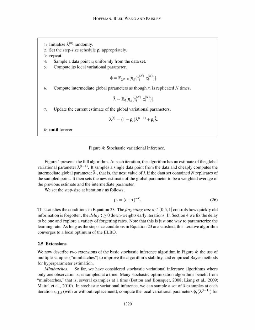
HOFFMAN, BLEI, WANG AND PAISLEY
1: Initialize λ(0) randomly.
2: Set the step-size schedule ρt appropriately.
3: repeat
4: Sample a data point xi uniformly from the data set.
5: Compute its local variational parameter,
φ = Eλ(t−1) [ηg(x(N)i ,z
(N)i )].
6: Compute intermediate global parameters as though xi is replicated N times,
λ = Eφ[ηg(x(N)i ,z
(N)i )].
7: Update the current estimate of the global variational parameters,
λ(t) = (1−ρt)λ(t−1)+ρt λ.
8: until forever
Figure 4: Stochastic variational inference.
Figure 4 presents the full algorithm. At each iteration, the algorithm has an estimate of the global
variational parameter λ(t−1). It samples a single data point from the data and cheaply computes the
intermediate global parameter λt , that is, the next value of λ if the data set contained N replicates of
the sampled point. It then sets the new estimate of the global parameter to be a weighted average of
the previous estimate and the intermediate parameter.
We set the step-size at iteration t as follows,
ρt = (t + τ)−κ. (26)
This satisfies the conditions in Equation 23. The forgetting rate κ∈ (0.5,1] controls how quickly old
information is forgotten; the delay τ≥ 0 down-weights early iterations. In Section 4 we fix the delay
to be one and explore a variety of forgetting rates. Note that this is just one way to parameterize the
learning rate. As long as the step size conditions in Equation 23 are satisfied, this iterative algorithm
converges to a local optimum of the ELBO.
2.5 Extensions
We now describe two extensions of the basic stochastic inference algorithm in Figure 4: the use of
multiple samples (“minibatches”) to improve the algorithm’s stability, and empirical Bayes methods
for hyperparameter estimation.
Minibatches. So far, we have considered stochastic variational inference algorithms where
only one observation xt is sampled at a time. Many stochastic optimization algorithms benefit from
“minibatches,” that is, several examples at a time (Bottou and Bousquet, 2008; Liang et al., 2009;
Mairal et al., 2010). In stochastic variational inference, we can sample a set of S examples at each
iteration xt,1:S (with or without replacement), compute the local variational parameters φs(λ(t−1)) for
1320
STOCHASTIC VARIATIONAL INFERENCE
each data point, compute the intermediate global parameters λs for each data point xts, and finally
average the λs variables in the update
λ(t) = (1−ρt)λ(t−1)+
ρt
S∑
s
λs.
The stochastic natural gradients associated with each point xs have expected value equal to the
gradient. Therefore, the average of these stochastic natural gradients has the same expectation and
the algorithm remains valid.
There are two reasons to use minibatches. The first reason is to amortize any computational
expenses associated with updating the global parameters across more data points; for example, if
the expected sufficient statistics of β are expensive to compute, using minibatches allows us to incur
that expense less frequently. The second reason is that it may help the algorithm to find better local
optima. Stochastic variational inference is guaranteed to converge to a local optimum but taking
large steps on the basis of very few data points may lead to a poor one. As we will see in Section 4,
using more of the data per update can help the algorithm.
Empirical Bayes estimation of hyperparameters. In some cases we may want to both estimate
the posterior of the hidden random variables β and z and obtain a point estimate of the values of the
hyperparameters α. One approach to fitting α is to try to maximize the marginal likelihood of the
data p(x |α), which is also known as empirical Bayes (Maritz and Lwin, 1989) estimation. Since we
cannot compute p(x |α) exactly, an approximate approach is to maximize the fitted variational lower
bound L over α. In the non-stochastic setting, α can be optimized by interleaving the coordinate
ascent updates in Figure 3 with an update for α that increases the ELBO. This is called variational
expectation-maximization.
In the stochastic setting, we update α simultaneously with λ. We can take a step in the direction
of the gradient of the noisy ELBO Lt (Equation 25) with respect to α, scaled by the step-size ρt ,
α(t) = α(t−1)+ρt∇αLt(λ(t−1),φ,α(t−1)).
Here λ(t−1) are the global parameters from the previous iteration and φ are the optimized local
parameters for the currently sampled data point. We can also replace the standard Euclidean gradient
with a natural gradient or Newton step.
3. Stochastic Variational Inference in Topic Models
We derived stochastic variational inference, a scalable inference algorithm that can be applied to
a large class of hierarchical Bayesian models. In this section we show how to use the general
algorithm of Section 2 to derive stochastic variational inference for two probabilistic topic models:
latent Dirichlet allocation (LDA) (Blei et al., 2003) and its Bayesian nonparametric counterpart, the
hierarchical Dirichlet process (HDP) topic model (Teh et al., 2006a).
Topic models are probabilistic models of document collections that use latent variables to en-
code recurring patterns of word use (Blei, 2012). Topic modeling algorithms are inference algo-
rithms; they uncover a set of patterns that pervade a collection and represent each document ac-
cording to how it exhibits them. These patterns tend to be thematically coherent, which is why
the models are called “topic models.” Topic models are used for both descriptive tasks, such as to
build thematic navigators of large collections of documents, and for predictive tasks, such as to aid
document classification. Topic models have been extended and applied in many domains.
1321
HOFFMAN, BLEI, WANG AND PAISLEY
Topic models assume that the words of each document arise from a mixture of multinomials.
Across a collection, the documents share the same mixture components (called topics). Each doc-
ument, however, is associated with its own mixture proportions (called topic proportions). In this
way, topic models represent documents heterogeneously—the documents share the same set of top-
ics, but each exhibits them to a different degree. For example, a document about sports and health
will be associated with the sports and health topics; a document about sports and business will be
associated with the sports and business topics. They both share the sports topic, but each combines
sports with a different topic. More generally, this is called mixed membership (Erosheva, 2003).
The central computational problem in topic modeling is posterior inference: Given a collection
of documents, what are the topics that it exhibits and how does each document exhibit them? In
practical applications of topic models, scale is important—these models promise an unsupervised
approach to organizing large collections of text (and, with simple adaptations, images, sound, and
other data). Thus they are a good testbed for stochastic variational inference.
More broadly, this section illustrates how to use the results from Section 2 to develop algorithms
for specific models. We will derive the algorithms in several steps: (1) we specify the model assump-
tions; (2) we derive the complete conditional distributions of the latent variables; (3) we form the
mean-field variational family; (4) we derive the corresponding stochastic inference algorithm. In
Section 4, we will report our empirical study of stochastic variational inference with these models.
3.1 Notation
We follow the notation of Blei et al. (2003).
• Observations are words, organized into documents. The nth word in the dth document is wdn.
Each word is an element in a fixed vocabulary of V terms.
• A topic βk is a distribution over the vocabulary. Each topic is a point on the V −1-simplex, a
positive vector of length V that sums to one. We denote the wth entry in the kth topic as βkw.
In LDA there are K topics; in the HDP topic model there are an infinite number of topics.
• Each document in the collection is associated with a vector of topic proportions θd , which
is a distribution over topics. In LDA θd is a point on the K − 1-simplex. In the HDP topic
model, θd is a point on the infinite simplex. (We give details about this below in Section 3.3.)
We denote the kth entry of the topic proportion vector θd as θdk.
• Each word in each document is assumed to have been drawn from a single topic. The topic
assignment zdn indexes the topic from which wdn is drawn.
The only observed variables are the words of the documents. The topics, topic proportions, and
topic assignments are latent variables.
3.2 Latent Dirichlet Allocation
LDA is the simplest topic model. It assumes that each document exhibits K topics with different
proportions. The generative process is
1. Draw topics βk ∼ Dirichlet(η, . . . ,η) for k ∈ {1, . . . ,K}.
2. For each document d ∈ {1, . . . ,D}:
1322
STOCHASTIC VARIATIONAL INFERENCE
Var
Type
Condit
ional
Par
amR
elev
ant
Expec
tati
ons
z dn
Mult
inom
ial
log
θd
k+
log
βk,w
dn
φd
nE[Z
k dn]=
φk d
n
θd
Dir
ichle
tα+
∑N n=
1z d
nγ d
E[l
og
θd
k]=
Ψ(γ
dk)−
∑K j=
1Ψ(γ
dj)
βk
Dir
ichle
tη+
∑D d=
1∑
N n=
1zk d
nw
dn
λk
E[l
og
βkv]=
Ψ(λ
kv)−
∑V y=
1Ψ(λ
ky)
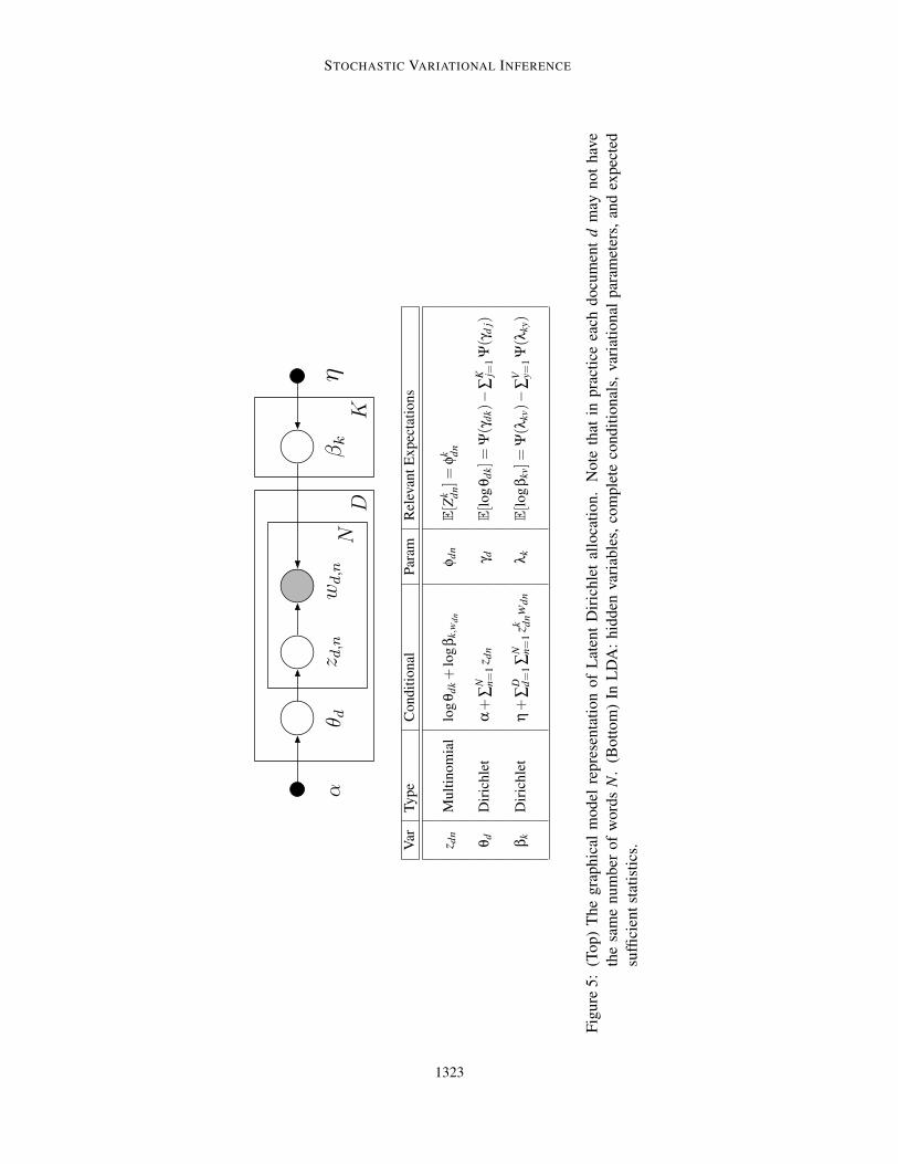
Fig
ure
5:
(Top)
The
gra
phic
alm
odel
repre
senta
tion
of
Lat
ent
Dir
ichle
tal
loca
tion.
Note
that
inpra
ctic
eea
chdocu
men
td
may
not
hav
e
the
sam
enum
ber
of
word
sN
.(B
ott
om
)In
LD
A:
hid
den
var
iable
s,co
mple
teco
ndit
ional
s,var
iati
onal
par
amet
ers,
and
expec
ted
suffi
cien
tst
atis
tics
.
1323
HOFFMAN, BLEI, WANG AND PAISLEY
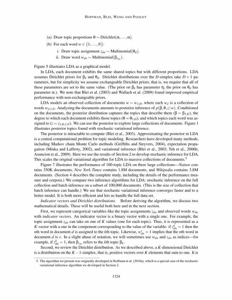
(a) Draw topic proportions θ ∼ Dirichlet(α, . . . ,α).
(b) For each word w ∈ {1, . . . ,N}:
i. Draw topic assignment zdn ∼ Multinomial(θd).
ii. Draw word wdn ∼ Multinomial(βzdn).
Figure 5 illustrates LDA as a graphical model.
In LDA, each document exhibits the same shared topics but with different proportions. LDA
assumes Dirichlet priors for βk and θd . Dirichlet distributions over the D-simplex take D+ 1 pa-
rameters, but for simplicity we assume exchangeable Dirichlet priors; that is, we require that all of
these parameters are set to the same value. (The prior on βk has parameter η; the prior on θd has
parameter α.). We note that Blei et al. (2003) and Wallach et al. (2009) found improved empirical
performance with non-exchangeable priors.
LDA models an observed collection of documents w = w1:D, where each wd is a collection of
words wd,1:N . Analyzing the documents amounts to posterior inference of p(β,θ,z |w). Conditioned
on the documents, the posterior distribution captures the topics that describe them (β = β1:K), the
degree to which each document exhibits those topics (θ = θ1:D), and which topics each word was as-
signed to (z = z1:D,1:N). We can use the posterior to explore large collections of documents. Figure 1
illustrates posterior topics found with stochastic variational inference.
The posterior is intractable to compute (Blei et al., 2003). Approximating the posterior in LDA
is a central computational problem for topic modeling. Researchers have developed many methods,
including Markov chain Monte Carlo methods (Griffiths and Steyvers, 2004), expectation propa-
gation (Minka and Lafferty, 2002), and variational inference (Blei et al., 2003; Teh et al., 2006b;
Asuncion et al., 2009). Here we use the results of Section 2 to develop stochastic inference for LDA.
This scales the original variational algorithm for LDA to massive collections of documents.5
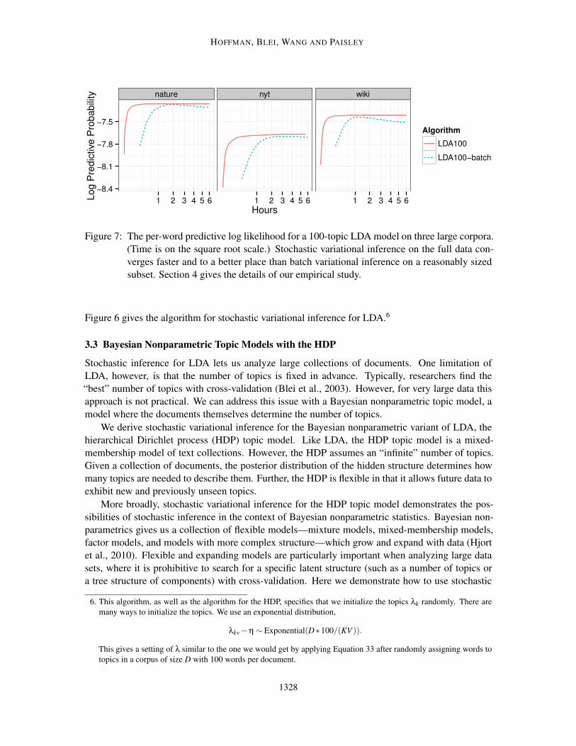
Figure 7 illustrates the performance of 100-topic LDA on three large collections—Nature con-
tains 350K documents, New York Times contains 1.8M documents, and Wikipedia contains 3.8M
documents. (Section 4 describes the complete study, including the details of the performance mea-
sure and corpora.) We compare two inference algorithms for LDA: stochastic inference on the full
collection and batch inference on a subset of 100,000 documents. (This is the size of collection that
batch inference can handle.) We see that stochastic variational inference converges faster and to a
better model. It is both more efficient and lets us handle the full data set.
Indicator vectors and Dirichlet distributions. Before deriving the algorithm, we discuss two
mathematical details. These will be useful both here and in the next section.
First, we represent categorical variables like the topic assignments zdn and observed words wdn
with indicator vectors. An indicator vector is a binary vector with a single one. For example, the
topic assignment zdn can take on one of K values (one for each topic). Thus, it is represented as a
K-vector with a one in the component corresponding to the value of the variable: if zkdn = 1 then the
nth word in document d is assigned to the kth topic. Likewise, wvdn = 1 implies that the nth word in
document d is v. In a slight abuse of notation, we will sometimes use wdn and zdn as indices—for
example, if zkdn = 1, then βzdn
refers to the kth topic βk.
Second, we review the Dirichlet distribution. As we described above, a K-dimensional Dirichlet
is a distribution on the K−1-simplex, that is, positive vectors over K elements that sum to one. It is
5. The algorithm we present was originally developed in Hoffman et al. (2010a), which is a special case of the stochastic
variational inference algorithm we developed in Section 2.
1324
STOCHASTIC VARIATIONAL INFERENCE
parameterized by a positive K-vector γ,
Dirichlet(θ;γ) =Γ(
∑Ki=1 γi
)
∏Ki=1 Γ(γi)
K
∏i=1
θγi−1,
where Γ(·) is the Gamma function, which is a real-valued generalization of the factorial function.
The expectation of the Dirichlet is its normalized parameter,
E[θk |γ] =γk
∑Ki=1 γi
.
The expectation of its log uses Ψ(·), which is the first derivative of the log Gamma function,
E[logθk |γ] = Ψ(γk)−Ψ(
∑Ki=1 γi
)
. (27)
This can be derived by putting the Dirichlet in exponential family form, noticing that logθ is the vec-
tor of sufficient statistics, and computing its expectation by taking the gradient of the log-normalizer
with respect to the natural parameter vector γ.
Complete conditionals and variational distributions. We specify the global and local variables
of LDA to place it in the stochastic variational inference setting of Section 2. In topic modeling,
the local context is a document d. The local observations are its observed words wd,1:N . The local
hidden variables are the topic proportions θd and the topic assignments zd,1:N . The global hidden
variables are the topics β1:K .
Recall from Section 2 that the complete conditional is the conditional distribution of a vari-
able given all of the other variables, hidden and observed. In mean-field variational inference, the
variational distributions of each variable are in the same family as the complete conditional.
We begin with the topic assignment zdn. The complete conditional of the topic assignment is a
multinomial,
p(zdn = k |θd,β1:K ,wdn) ∝ exp{logθdk + logβk,wdn}. (28)
Thus its variational distribution is a multinomial q(zdn) = Multinomial(φdn), where the variational
parameter φdn is a point on the K − 1-simplex. Per the mean-field approximation, each observed
word is endowed with a different variational distribution for its topic assignment, allowing different
words to be associated with different topics.
The complete conditional of the topic proportions is a Dirichlet,
p(θd |zd) = Dirichlet(
α+∑Nn=1 zdn
)
. (29)
Since zdn is an indicator vector, the kth element of the parameter to this Dirichlet is the sum of the
hyperparameter α and the number of words assigned to topic k in document d. Note that, although
we have assumed an exchangeable Dirichlet prior, when we condition on z the conditional p(θd|zd)is a non-exchangeable Dirichlet.
With this conditional, the variational distribution of the topic proportions is also Dirichlet q(θd)=Dirichlet(γd), where γd is a K-vector Dirichlet parameter. There is a different variational Dirichlet
parameter for each document, allowing different documents to be associated with different topics in
different proportions.
These are local hidden variables. The complete conditionals only depend on other variables in
the local context (i.e., the document) and the global variables; they do not depend on variables from
other documents.
1325

HOFFMAN, BLEI, WANG AND PAISLEY
Finally, the complete conditional for the topic βk is also a Dirichlet,
p(βk |z,w) = Dirichlet(
η+∑Dd=1 ∑N
n=1 zkdnwdn
)
. (30)
The vth element of the parameter to the Dirichlet conditional for topic k is the sum of the hyper-
parameter η and the number of times that the term v was assigned to topic k. This is a global
variable—its complete conditional depends on the words and topic assignments of the entire collec-
tion.
The variational distribution for each topic is a V -dimensional Dirichlet,
q(βk) = Dirichlet(λk).
As we will see in the next section, the traditional variational inference algorithm for LDA is ineffi-
cient with large collections of documents. The root of this inefficiency is the update for the topic
parameter λk, which (from Equation 30) requires summing over variational parameters for every
word in the collection.
Batch variational inference.
With the complete conditionals in hand, we now derive the coordinate ascent variational infer-
ence algorithm, that is, the batch inference algorithm of Figure 3. We form each coordinate update
by taking the expectation of the natural parameter of the complete conditional. This is the stepping
stone to stochastic variational inference.
The variational parameters are the global per-topic Dirichlet parameters λ1:K , local per-document
Dirichlet parameters γ1:D, and local per-word multinomial parameters φ1:D,1:N . Coordinate ascent
variational inference iterates between updating all of the local variational parameters (Equation 16)
and updating the global variational parameters (Equation 15).
We update each document d’s local variational in a local coordinate ascent routine, iterating
between updating each word’s topic assignment and the per-document topic proportions,
φkdn ∝ exp{Ψ(γdk)+Ψ(λk,wdn
)−Ψ(∑v λkv)} for n ∈ {1, . . . ,N}, (31)
γd = α+∑Nn=1 φdn. (32)
These updates derive from taking the expectations of the natural parameters of the complete con-
ditionals in Equation 28 and Equation 29. (We then map back to the usual parameterization of
the multinomial.) For the update on the topic assignment, we have used the Dirichlet expectations
in Equation 27. For the update on the topic proportions, we have used that the expectation of an
indicator is its probability, Eq[zkdn] = φk
dn.
After finding variational parameters for each document, we update the variational Dirichlet for
each topic,
λk = η+∑Dd=1 ∑N
n=1 φkdnwdn. (33)
This update depends on the variational parameters φ from every document.
Batch inference is inefficient for large collections of documents. Before updating the topics
λ1:K , we compute the local variational parameters for every document. This is particularly wasteful
in the beginning of the algorithm when, before completing the first iteration, we must analyze every
document with randomly initialized topics.
Stochastic variational inference
1326

STOCHASTIC VARIATIONAL INFERENCE
1: Initialize λ(0) randomly.
2: Set the step-size schedule ρt appropriately.
3: repeat
4: Sample a document wd uniformly from the data set.
5: Initialize γdk = 1, for k ∈ {1, . . . ,K}.
6: repeat
7: For n ∈ {1, . . . ,N} set
φkdn ∝ exp{E[logθdk]+E[logβk,wdn
]} , k ∈ {1, . . . ,K}.
8: Set γd = α+∑n φdn.
9: until local parameters φdn and γd converge.
10: For k ∈ {1, . . . ,K} set intermediate topics
λk = η+DN
∑n=1
φkdnwdn.
11: Set λ(t) = (1−ρt)λ(t−1)+ρt λ.
12: until forever
Figure 6: Stochastic variational inference for LDA. The relevant expectations for each update are
found in Figure 5.
Stochastic variational inference provides a scalable method for approximate posterior inference
in LDA. The global variational parameters are the topic Dirichlet parameters λk; the local variational
parameters are the per-document topic proportion Dirichlet parameters γd and the per-word topic
assignment multinomial parameters φdn.
We follow the general algorithm of Figure 4. Let λ(t) be the topics at iteration t. At each iteration
we sample a document d from the collection. In the local phase, we compute optimal variational
parameters by iterating between updating the per-document parameters γd (Equation 32) and φd,1:N
(Equation 31). This is the same subroutine as in batch inference, though here we only analyze one
randomly chosen document.
In the global phase we use these fitted local variational parameters to form intermediate topics,
λk = η+D∑Nn=1 φk
dnwdn.
This comes from applying Equation 33 to a hypothetical corpus containing D replicates of document
d. We then set the topics at the next iteration to be a weighted combination of the intermediate topics
and current topics,
λ(t+1)k = (1−ρt)λ
(t)k +ρt λk.
1327
HOFFMAN, BLEI, WANG AND PAISLEY
nature nyt wiki
−8.4
−8.1
−7.8
−7.5
1 2 3 4 5 6 1 2 3 4 5 6 1 2 3 4 5 6
Hours
Log P
redic
tive P
robabili
ty
Algorithm
LDA100
LDA100−batch
Figure 7: The per-word predictive log likelihood for a 100-topic LDA model on three large corpora.
(Time is on the square root scale.) Stochastic variational inference on the full data con-
verges faster and to a better place than batch variational inference on a reasonably sized
subset. Section 4 gives the details of our empirical study.
Figure 6 gives the algorithm for stochastic variational inference for LDA.6
3.3 Bayesian Nonparametric Topic Models with the HDP
Stochastic inference for LDA lets us analyze large collections of documents. One limitation of
LDA, however, is that the number of topics is fixed in advance. Typically, researchers find the
“best” number of topics with cross-validation (Blei et al., 2003). However, for very large data this
approach is not practical. We can address this issue with a Bayesian nonparametric topic model, a
model where the documents themselves determine the number of topics.
We derive stochastic variational inference for the Bayesian nonparametric variant of LDA, the
hierarchical Dirichlet process (HDP) topic model. Like LDA, the HDP topic model is a mixed-
membership model of text collections. However, the HDP assumes an “infinite” number of topics.
Given a collection of documents, the posterior distribution of the hidden structure determines how
many topics are needed to describe them. Further, the HDP is flexible in that it allows future data to
exhibit new and previously unseen topics.
More broadly, stochastic variational inference for the HDP topic model demonstrates the pos-
sibilities of stochastic inference in the context of Bayesian nonparametric statistics. Bayesian non-
parametrics gives us a collection of flexible models—mixture models, mixed-membership models,
factor models, and models with more complex structure—which grow and expand with data (Hjort
et al., 2010). Flexible and expanding models are particularly important when analyzing large data
sets, where it is prohibitive to search for a specific latent structure (such as a number of topics or
a tree structure of components) with cross-validation. Here we demonstrate how to use stochastic
6. This algorithm, as well as the algorithm for the HDP, specifies that we initialize the topics λk randomly. There are
many ways to initialize the topics. We use an exponential distribution,
λkv −η ∼ Exponential(D∗100/(KV )).
This gives a setting of λ similar to the one we would get by applying Equation 33 after randomly assigning words to
topics in a corpus of size D with 100 words per document.
1328
STOCHASTIC VARIATIONAL INFERENCE
inference in the context of a simple Bayesian nonparametric topic model. In other work, we built
on this algorithm to give scalable inference methods for Bayesian nonparametric models of topic
correlation (Paisley et al., 2012b) and tree structures of topics (Paisley et al., 2012c).
This section is organized as follows. We first give some background on the Dirichlet process
and its definition via Sethuraman’s stick breaking construction, which is a distribution on the infinite
simplex. We then show how to use this construction to form the HDP topic model and how to use
stochastic variational inference to approximate the posterior.7
The stick-breaking construction of the Dirichlet process. Bayesian nonparametric (BNP) meth-
ods use distributions of distributions, placing flexible priors on the shape of the data-generating
density function. BNP models draw a distribution from that prior and then independently draw data
from that random distribution. Data analysis proceeds by evaluating the posterior distribution of the
(random) distribution from which the data were drawn. Because of the flexible prior, that posterior
can potentially have mass on a wide variety of distribution shapes. For a reviews of BNP methods,
see the edited volume of Hjort et al. (2010) and the tutorial of Gershman and Blei (2012).
The most common BNP prior is the Dirichlet process (DP). The Dirichlet process is parame-
terized by a base distribution G0 (which may be either continuous or discrete) and a non-negative
scaling factor α. These are used to form a distribution over discrete distributions, that is, over dis-
tributions that place their mass on a countably infinite set of atoms. The locations of the atoms are
independently drawn from the base distribution G0 and the closeness of the probabilities to G0 is
determined by the scaling factor α. When α is small, more mass is placed on fewer atoms, and
the draw will likely look very different from G0; when α is large, the mass is spread around many
atoms, and the draw will more closely resemble the base distribution.
There are several representations of the Dirichlet process. For example, it is a normalized
gamma process (Ferguson, 1973), and its marginalization gives the Chinese restaurant process (Pit-
man, 2002). We will focus on its definition via Sethuraman’s stick breaking construction (Sethura-
man, 1994). The stick-breaking construction explicitly defines the distribution of the probabilities
that make up a random discrete distribution. It is the gateway to variational inference in Bayesian
nonparametric models (Blei and Jordan, 2006).
Let G∼DP(α,G0) be drawn from a Dirichlet process prior. It is a discrete distribution with mass
on an infinite set of atoms. Let βk be the atoms in this distribution and σk be their corresponding
probabilities. We can write G as
G =∞
∑k=1
σkδβk.
The atoms are drawn independently from G0. The stick-breaking construction specifies the distribu-
tion of their probabilities.
The stick-breaking construction uses an infinite collection of beta-distributed random variables.
Recall that the beta is a distribution on (0,1) and define the following collection,
vi ∼ Beta(1,α) i ∈ {1,2,3, . . .}.
These variables combine to form a point on the infinite simplex. Imagine a stick of unit length.
Break off the proportion of the stick given by v1, call it σ1, and set it aside. From the remainder (of
length 1−σ1) break off the proportion given by v2, call it σ2, and set it aside. The remainder of
7. This algorithm first appeared in Wang et al. (2011). Here we place it in the more general context of Section 2 and
relate it to stochastic inference for LDA.
1329

HOFFMAN, BLEI, WANG AND PAISLEY
the stick is now 1−σ2 −σ1 = (1− v1)(1− v2). Repeat this process for the infinite set of vi. The
resulting stick lengths σi will sum to one.
More formally, we define the function σi to take the collection of realized vi variables and to
return the stick length of the ith component,
σi(v) = vi ∏i−1j=1(1− v j),
and note that ∑∞i=1 σi(v) = 1. We call vi the ith breaking proportion.
Combining these steps, we form the distribution G according to the following process,
βi ∼ G0 i ∈ {1,2,3, . . .},
vi ∼ Beta(1,α) i ∈ {1,2,3, . . .},
G = ∑∞i=1 σi(v)δβi
.
In the random distribution G the ith atom βi is an independent draw from G0 and it has proba-
bility given by the ith stick length σi(v). Sethuraman (1994) showed that the distribution of G is
DP(α,G0).The most important property of G is the “clustering” property. Even though G places mass on
a countably infinite set of atoms, N draws from G will tend to exhibit only a small number of them.
(How many depends on the scalar α, as we described above.) Formally, this is most easily seen
via other perspectives on the DP (Ferguson, 1973; Blackwell and MacQueen, 1973; Pitman, 2002),
though it can be seen intuitively with the stick-breaking construction. The intuition is that as α gets
smaller more of the stick is absorbed in the first break locations because the breaking proportions
are drawn from Beta(1,α). Thus, those atoms associated with the first breaks of the stick will have
larger mass in the distribution G, and that in turn encourages draws from the distribution to realize
fewer individual atoms. In general, the first break locations tend to be larger than the later break
locations. This property is called size biasedness.
The HDP topic model. We now construct a Bayesian nonparametric topic model that has
an “infinite” number of topics. The hierarchical Dirichlet process topic model couples a set of
document-level DPs via a single top-level DP (Teh et al., 2006a). The base distribution H of the
top-level DP is a symmetric Dirichlet over the vocabulary simplex—its atoms are topics. We draw
once from this DP, G0 ∼ DP(ω,H). In the second level, we use G0 as a base measure to a document-
level DP, Gd ∼ DP(α,G0). We draw the words of each document d from topics from Gd . The
consequence of this two-level construction is that all documents share the same collection of topics
but exhibit them with different proportions.
We construct the HDP topic model using a stick-breaking construction at each level—one at the
document level and one at the corpus level.8 The generative process of the HDP topic model is as
follows.
1. Draw an infinite number of topics, βk ∼ Dirichlet(η) for k ∈ {1,2,3, . . .}.
2. Draw corpus breaking proportions, vk ∼ Beta(1,ω) for k ∈ {1,2,3, . . .}.
3. For each document d:
8. See the original HDP paper of Teh et al. (2006a) for other constructions of the HDP—the random measure con-
struction, the construction by the Chinese restaurant franchise, and an alternative stick-breaking construction. This
construction was mentioned by Fox et al. (2008). We used it for the HDP in Wang et al. (2011).
1330

STOCHASTIC VARIATIONAL INFERENCE
(a) Draw document-level topic indices, cdi ∼ Multinomial(σ(v)) for i ∈ {1,2,3, . . .}.
(b) Draw document breaking proportions, πdi ∼ Beta(1,α) for i ∈ {1,2,3, . . .}.
(c) For each word n:
i. Draw topic assignment zdn ∼ Multinomial(σ(πd)).
ii. Draw word wn ∼ Multinomial(βcd,zdn).
Figure 8 illustrates this process as a graphical model.
In this construction, topics βk are drawn as in LDA (Step 1). Corpus-level breaking proportions
v (Step 2) define a probability distribution on these topics, which indicates their relative prevalence
in the corpus. At the document level, breaking proportions πd create a set of probabilities (Step 3b)
and topic indices cd , drawn from σ(v), attach each document-level stick length to a topic (Step 3a).
This creates a document-level distribution over topics, and words are then drawn as for LDA (Step
3c).
The posterior distribution of the HDP topic model gives a mixed-membership decomposition
of a corpus where the number of topics is unknown in advance and unbounded. However, it is not
possible to compute the posterior. Approximate posterior inference for BNP models in general is
an active field of research (Escobar and West, 1995; Neal, 2000; Blei and Jordan, 2006; Teh et al.,
2007).
The advantage of our construction over others is that it meets the conditions of Section 2. All
the complete conditionals are in exponential families in closed form, and it neatly separates global
variables from local variables. The global variables are topics and corpus-level breaking proportions;
the local variables are document-level topic indices and breaking proportions. Following the same
procedure as for LDA, we now derive stochastic variational inference for the HDP topic model.
Complete conditionals and variational distributions. We form the complete conditional distri-
butions of all variables in the HDP topic model. We begin with the latent indicator variables,
p(zidn = 1|πd ,β1:K ,wdn,cd) ∝ exp{logσi(πd)+∑∞
k=1 ckdi logβk,wdn
},
p(ckdi = 1|v,β1:K ,wd ,zd) ∝ exp{logσk(v)+∑N
n=1 zidn logβk,wdn
}.
Note the interaction between the two levels of latent indicators. In LDA the ith component of the
topic proportions points to the ith topic. Here we must account for the topic index cdi, which is a
random variable that points to one of the topics.
This interaction between indicators is also seen in the conditionals for the topics,
p(βk|z,c,w) = Dirichlet(
η+∑Dd=1 ∑∞
i=1 ckdi ∑N
n=1 zidnwdn
)
.
The innermost sum collects the sufficient statistics for words in the dth document that are allocated
to the ith local component index. However, these statistics are only kept when the ith topic index
cdi points to the kth global topic.
The full conditionals for the breaking proportions follow those of a standard stick-breaking
construction (Blei and Jordan, 2006),
p(vk|c) = Beta(
1+∑Dd=1 ∑∞
i=1 ckdi , ω+∑D
d=1 ∑∞i=1 ∑ j>k c
j
di
)
,
p(πdi|zd) = Beta(
1+∑Nn=1 zi
dn , α+∑Nn=1 ∑ j>i z
j
dn
)
.
1331
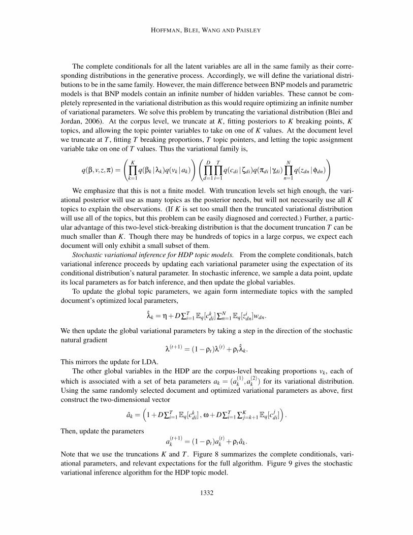
HOFFMAN, BLEI, WANG AND PAISLEY
The complete conditionals for all the latent variables are all in the same family as their corre-
sponding distributions in the generative process. Accordingly, we will define the variational distri-
butions to be in the same family. However, the main difference between BNP models and parametric
models is that BNP models contain an infinite number of hidden variables. These cannot be com-
pletely represented in the variational distribution as this would require optimizing an infinite number
of variational parameters. We solve this problem by truncating the variational distribution (Blei and
Jordan, 2006). At the corpus level, we truncate at K, fitting posteriors to K breaking points, K
topics, and allowing the topic pointer variables to take on one of K values. At the document level
we truncate at T , fitting T breaking proportions, T topic pointers, and letting the topic assignment
variable take on one of T values. Thus the variational family is,
q(β,v,z,π) =
(
K
∏k=1
q(βk |λk)q(vk |ak)
)(
D
∏d=1
T
∏i=1
q(cdi |ζdi)q(πdi |γdi)N
∏n=1
q(zdn |φdn)
)
We emphasize that this is not a finite model. With truncation levels set high enough, the vari-
ational posterior will use as many topics as the posterior needs, but will not necessarily use all K
topics to explain the observations. (If K is set too small then the truncated variational distribution
will use all of the topics, but this problem can be easily diagnosed and corrected.) Further, a partic-
ular advantage of this two-level stick-breaking distribution is that the document truncation T can be
much smaller than K. Though there may be hundreds of topics in a large corpus, we expect each
document will only exhibit a small subset of them.
Stochastic variational inference for HDP topic models. From the complete conditionals, batch
variational inference proceeds by updating each variational parameter using the expectation of its
conditional distribution’s natural parameter. In stochastic inference, we sample a data point, update
its local parameters as for batch inference, and then update the global variables.
To update the global topic parameters, we again form intermediate topics with the sampled
document’s optimized local parameters,
λk = η+D∑Ti=1Eq[c
kdi]∑
Nn=1Eq[z
idn]wdn.
We then update the global variational parameters by taking a step in the direction of the stochastic
natural gradient
λ(t+1) = (1−ρt)λ(t)+ρt λk.
This mirrors the update for LDA.
The other global variables in the HDP are the corpus-level breaking proportions vk, each of
which is associated with a set of beta parameters ak = (a(1)k ,a
(2)k ) for its variational distribution.
Using the same randomly selected document and optimized variational parameters as above, first
construct the two-dimensional vector
ak =(
1+D∑Ti=1Eq[c
kdi] , ω+D∑T
i=1 ∑Kj=k+1Eq[c
j
di])
.
Then, update the parameters
a(t+1)k = (1−ρt)a
(t)k +ρt ak.
Note that we use the truncations K and T . Figure 8 summarizes the complete conditionals, vari-
ational parameters, and relevant expectations for the full algorithm. Figure 9 gives the stochastic
variational inference algorithm for the HDP topic model.
1332
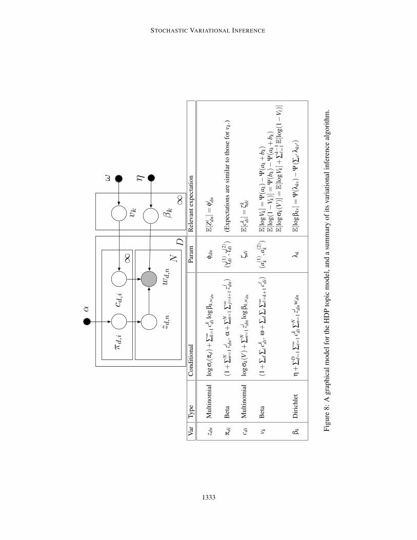
STOCHASTIC VARIATIONAL INFERENCE
Var
Type
Condit
ional
Par
amR
elev
ant
expec
tati
on
z dn
Mult
inom
ial
log
σi(
πd)+
∑∞ k=
1ck d
ilo
gβ
k,w
dn
φd
nE[Z
i dn]=
φi d
n
πd
iB
eta
(1+
∑N n=
1zi d
n,
α+
∑N n=
1∑
∞ j=i+
1z
j dn)
(γ(1)
di,γ
(2)
di)
(Expec
tati
ons
are
sim
ilar
toth
ose
for
v k.)
c di
Mult
inom
ial
log
σk(V
)+
∑N n=
1zi d
nlo
gβ
k,w
dn
ζd
iE[c
k di]=
ζk d
i
v kB
eta
(1+
∑d
∑ick d
i,ω+
∑d
∑i∑
∞ ℓ=k+
1cℓ d
i)(a
(1)
k,a
(2)
k)
E[l
og
Vk]=
Ψ(a
k)−
Ψ(a
k+
bk)
E[l
og(1
−V
k)]=
Ψ(b
k)−
Ψ(a
k+
bk)
E[l
og
σk(V
)]=E[l
og
Vk]+
∑k−
1ℓ=
1E[l
og(1
−Vℓ)]
βk
Dir
ichle
tη+
∑D d=
1∑
∞ i=1
ck di∑
N n=
1zi d
nw
dn
λk
E[l
og
βkv]=
Ψ(λ
kv)−
Ψ( ∑
v′λ
kv′)
Fig
ure
8:
Agra
phic
alm
odel
for
the
HD
Pto
pic
model
,an
da
sum
mar
yof
its
var
iati
onal
infe
rence
algori
thm
.
1333
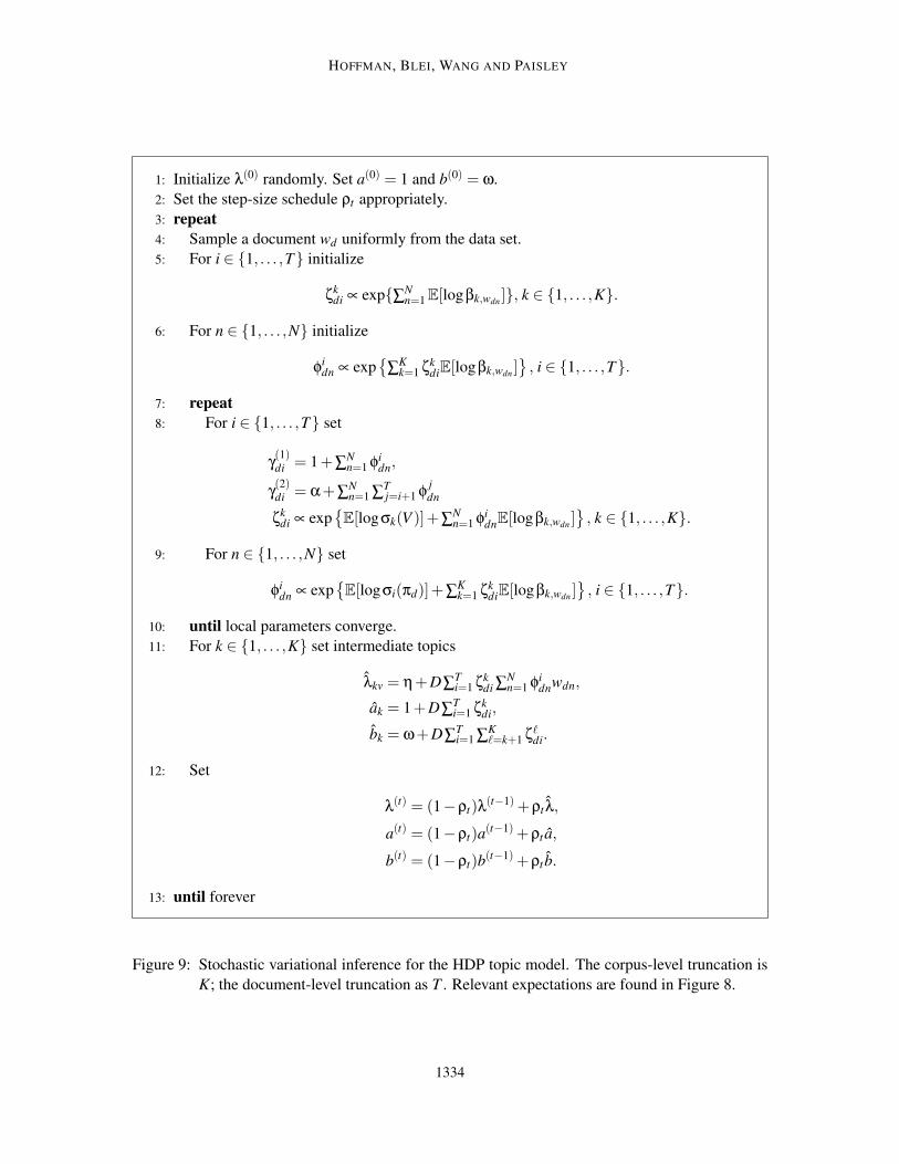
HOFFMAN, BLEI, WANG AND PAISLEY
1: Initialize λ(0) randomly. Set a(0) = 1 and b(0) = ω.
2: Set the step-size schedule ρt appropriately.
3: repeat
4: Sample a document wd uniformly from the data set.
5: For i ∈ {1, . . . ,T} initialize
ζkdi ∝ exp{∑N
n=1E[logβk,wdn]}, k ∈ {1, . . . ,K}.
6: For n ∈ {1, . . . ,N} initialize
φidn ∝ exp
{
∑Kk=1 ζk
diE[logβk,wdn]}
, i ∈ {1, . . . ,T}.
7: repeat
8: For i ∈ {1, . . . ,T} set
γ(1)di = 1+∑N
n=1 φidn,
γ(2)di = α+∑N
n=1 ∑Tj=i+1 φ
j
dn
ζkdi ∝ exp
{
E[logσk(V )]+∑Nn=1 φi
dnE[logβk,wdn]}
, k ∈ {1, . . . ,K}.
9: For n ∈ {1, . . . ,N} set
φidn ∝ exp
{
E[logσi(πd)]+∑Kk=1 ζk
diE[logβk,wdn]}
, i ∈ {1, . . . ,T}.
10: until local parameters converge.
11: For k ∈ {1, . . . ,K} set intermediate topics
λkv = η+D∑Ti=1 ζk
di ∑Nn=1 φi
dnwdn,
ak = 1+D∑Ti=1 ζk
di,
bk = ω+D∑Ti=1 ∑K
ℓ=k+1 ζℓdi.
12: Set
λ(t) = (1−ρt)λ(t−1)+ρt λ,
a(t) = (1−ρt)a(t−1)+ρt a,
b(t) = (1−ρt)b(t−1)+ρt b.
13: until forever
Figure 9: Stochastic variational inference for the HDP topic model. The corpus-level truncation is
K; the document-level truncation as T . Relevant expectations are found in Figure 8.
1334

STOCHASTIC VARIATIONAL INFERENCE
nature nyt wiki
−8.0
−7.6
−7.2
5 10 20 30 5 10 20 30 5 10 20 30
Hours
Log P
redic
tive P
robabili
ty
Algorithm
HDP
HDP−batch
Figure 10: The per-word predictive log likelihood for an HDP model on three large corpora. (Time
is on the square root scale.) As for LDA, stochastic variational inference on the full data
converges faster and to a better place than batch variational inference on a reasonably
sized subset. Section 4 gives the details of our empirical study.
Stochastic inference versus batch inference for the HDP. Figure 10 illustrates the performance
of the HDP topic model on the same three large collections as in Figure 7. As with LDA, stochastic
variational inference for the HDP converges faster and to a better model.
4. Empirical Study
In this section we study the empirical performance and effectiveness of stochastic variational infer-
ence for latent Dirichlet allocation (LDA) and the hierarchical Dirichlet process (HDP) topic model.
With these algorithms, we can apply and compare these models with very large collections of docu-
ments. We also investigate how the forgetting rate κ and mini-batch size S influence the algorithms.
Finally, we compare stochastic variational inference to the traditional batch variational inference
algorithm.9
Data. We evaluated our algorithms on three collections of documents. For each collection, we
computed a vocabulary by removing stop words, rare words, and very frequent words. The data are
as follows.
• Nature: This collection contains 350,000 documents from the journal Nature (spanning the
years 1869–2008). After processing, it contains 58M observed words from a vocabulary of
4,200 terms.
• New York Times: This collection contains 1.8M documents from the New York Times (span-
ning the years 1987–2007). After processing, this data contains 461M observed words from
a vocabulary of 8,000 terms.
9. We implemented all algorithms in Python using the NumPy and SciPy packages, making the implementations as
similar as possible. Links to these implementations are available on the web at http://www.cs.princeton.edu/
~blei/topicmodeling.html.
1335
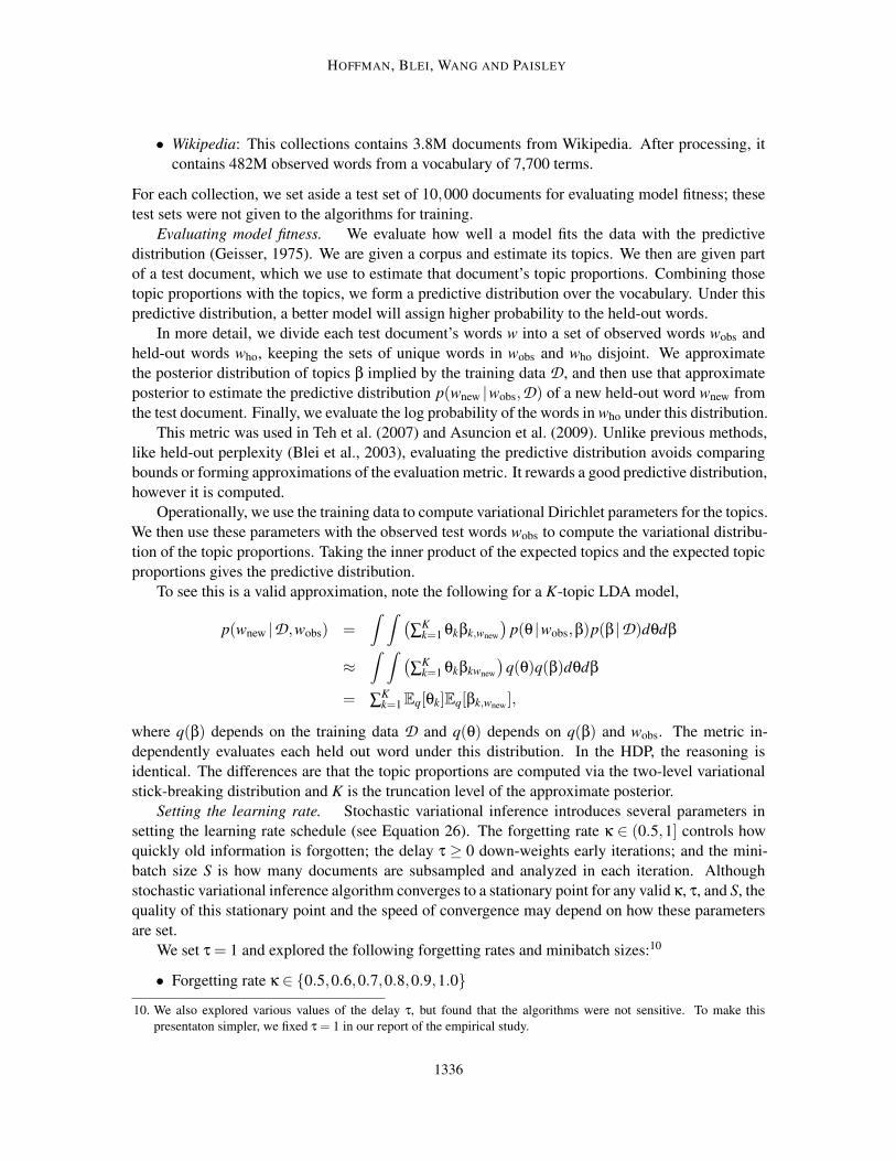
HOFFMAN, BLEI, WANG AND PAISLEY
• Wikipedia: This collections contains 3.8M documents from Wikipedia. After processing, it
contains 482M observed words from a vocabulary of 7,700 terms.
For each collection, we set aside a test set of 10,000 documents for evaluating model fitness; these
test sets were not given to the algorithms for training.
Evaluating model fitness. We evaluate how well a model fits the data with the predictive
distribution (Geisser, 1975). We are given a corpus and estimate its topics. We then are given part
of a test document, which we use to estimate that document’s topic proportions. Combining those
topic proportions with the topics, we form a predictive distribution over the vocabulary. Under this
predictive distribution, a better model will assign higher probability to the held-out words.
In more detail, we divide each test document’s words w into a set of observed words wobs and
held-out words who, keeping the sets of unique words in wobs and who disjoint. We approximate
the posterior distribution of topics β implied by the training data D , and then use that approximate
posterior to estimate the predictive distribution p(wnew |wobs,D) of a new held-out word wnew from
the test document. Finally, we evaluate the log probability of the words in who under this distribution.
This metric was used in Teh et al. (2007) and Asuncion et al. (2009). Unlike previous methods,
like held-out perplexity (Blei et al., 2003), evaluating the predictive distribution avoids comparing
bounds or forming approximations of the evaluation metric. It rewards a good predictive distribution,
however it is computed.
Operationally, we use the training data to compute variational Dirichlet parameters for the topics.
We then use these parameters with the observed test words wobs to compute the variational distribu-
tion of the topic proportions. Taking the inner product of the expected topics and the expected topic
proportions gives the predictive distribution.
To see this is a valid approximation, note the following for a K-topic LDA model,
p(wnew |D,wobs) =∫ ∫
(
∑Kk=1 θkβk,wnew
)
p(θ |wobs,β)p(β |D)dθdβ
≈∫ ∫
(
∑Kk=1 θkβkwnew
)
q(θ)q(β)dθdβ
= ∑Kk=1Eq[θk]Eq[βk,wnew
],
where q(β) depends on the training data D and q(θ) depends on q(β) and wobs. The metric in-
dependently evaluates each held out word under this distribution. In the HDP, the reasoning is
identical. The differences are that the topic proportions are computed via the two-level variational
stick-breaking distribution and K is the truncation level of the approximate posterior.
Setting the learning rate. Stochastic variational inference introduces several parameters in
setting the learning rate schedule (see Equation 26). The forgetting rate κ ∈ (0.5,1] controls how
quickly old information is forgotten; the delay τ ≥ 0 down-weights early iterations; and the mini-
batch size S is how many documents are subsampled and analyzed in each iteration. Although
stochastic variational inference algorithm converges to a stationary point for any valid κ, τ, and S, the
quality of this stationary point and the speed of convergence may depend on how these parameters
are set.
We set τ = 1 and explored the following forgetting rates and minibatch sizes:10
• Forgetting rate κ ∈ {0.5,0.6,0.7,0.8,0.9,1.0}
10. We also explored various values of the delay τ, but found that the algorithms were not sensitive. To make this
presentaton simpler, we fixed τ = 1 in our report of the empirical study.
1336
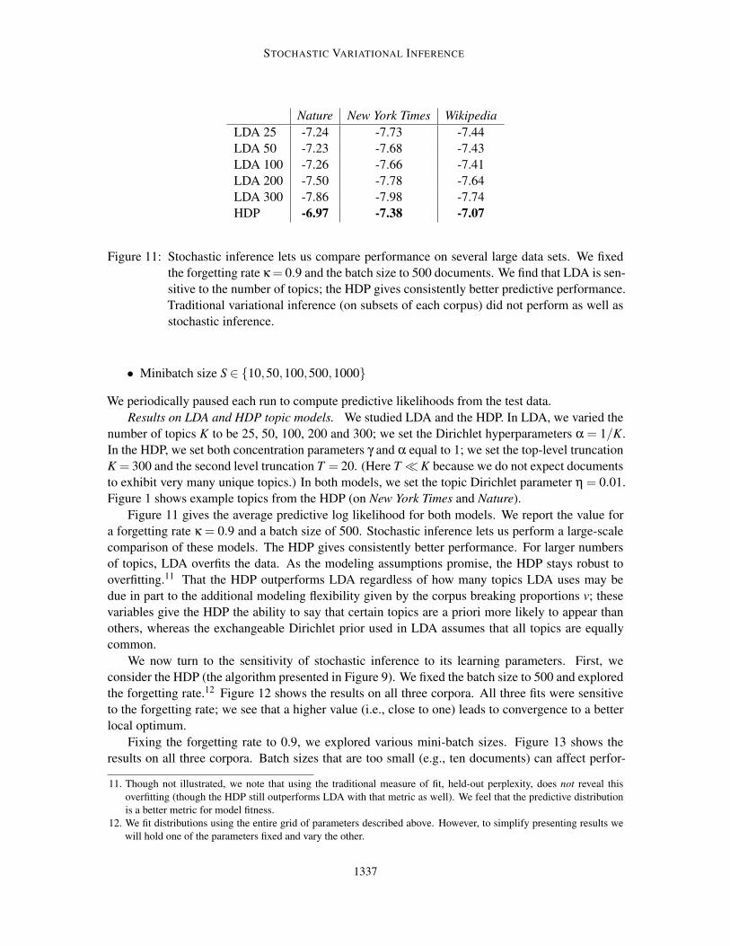
STOCHASTIC VARIATIONAL INFERENCE
Nature New York Times Wikipedia
LDA 25 -7.24 -7.73 -7.44
LDA 50 -7.23 -7.68 -7.43
LDA 100 -7.26 -7.66 -7.41
LDA 200 -7.50 -7.78 -7.64
LDA 300 -7.86 -7.98 -7.74
HDP -6.97 -7.38 -7.07
Figure 11: Stochastic inference lets us compare performance on several large data sets. We fixed
the forgetting rate κ = 0.9 and the batch size to 500 documents. We find that LDA is sen-
sitive to the number of topics; the HDP gives consistently better predictive performance.
Traditional variational inference (on subsets of each corpus) did not perform as well as
stochastic inference.
• Minibatch size S ∈ {10,50,100,500,1000}
We periodically paused each run to compute predictive likelihoods from the test data.
Results on LDA and HDP topic models. We studied LDA and the HDP. In LDA, we varied the
number of topics K to be 25, 50, 100, 200 and 300; we set the Dirichlet hyperparameters α = 1/K.
In the HDP, we set both concentration parameters γ and α equal to 1; we set the top-level truncation
K = 300 and the second level truncation T = 20. (Here T ≪ K because we do not expect documents
to exhibit very many unique topics.) In both models, we set the topic Dirichlet parameter η = 0.01.
Figure 1 shows example topics from the HDP (on New York Times and Nature).
Figure 11 gives the average predictive log likelihood for both models. We report the value for
a forgetting rate κ = 0.9 and a batch size of 500. Stochastic inference lets us perform a large-scale
comparison of these models. The HDP gives consistently better performance. For larger numbers
of topics, LDA overfits the data. As the modeling assumptions promise, the HDP stays robust to
overfitting.11 That the HDP outperforms LDA regardless of how many topics LDA uses may be
due in part to the additional modeling flexibility given by the corpus breaking proportions v; these
variables give the HDP the ability to say that certain topics are a priori more likely to appear than
others, whereas the exchangeable Dirichlet prior used in LDA assumes that all topics are equally
common.
We now turn to the sensitivity of stochastic inference to its learning parameters. First, we
consider the HDP (the algorithm presented in Figure 9). We fixed the batch size to 500 and explored
the forgetting rate.12 Figure 12 shows the results on all three corpora. All three fits were sensitive
to the forgetting rate; we see that a higher value (i.e., close to one) leads to convergence to a better
local optimum.
Fixing the forgetting rate to 0.9, we explored various mini-batch sizes. Figure 13 shows the
results on all three corpora. Batch sizes that are too small (e.g., ten documents) can affect perfor-
11. Though not illustrated, we note that using the traditional measure of fit, held-out perplexity, does not reveal this
overfitting (though the HDP still outperforms LDA with that metric as well). We feel that the predictive distribution
is a better metric for model fitness.
12. We fit distributions using the entire grid of parameters described above. However, to simplify presenting results we
will hold one of the parameters fixed and vary the other.
1337
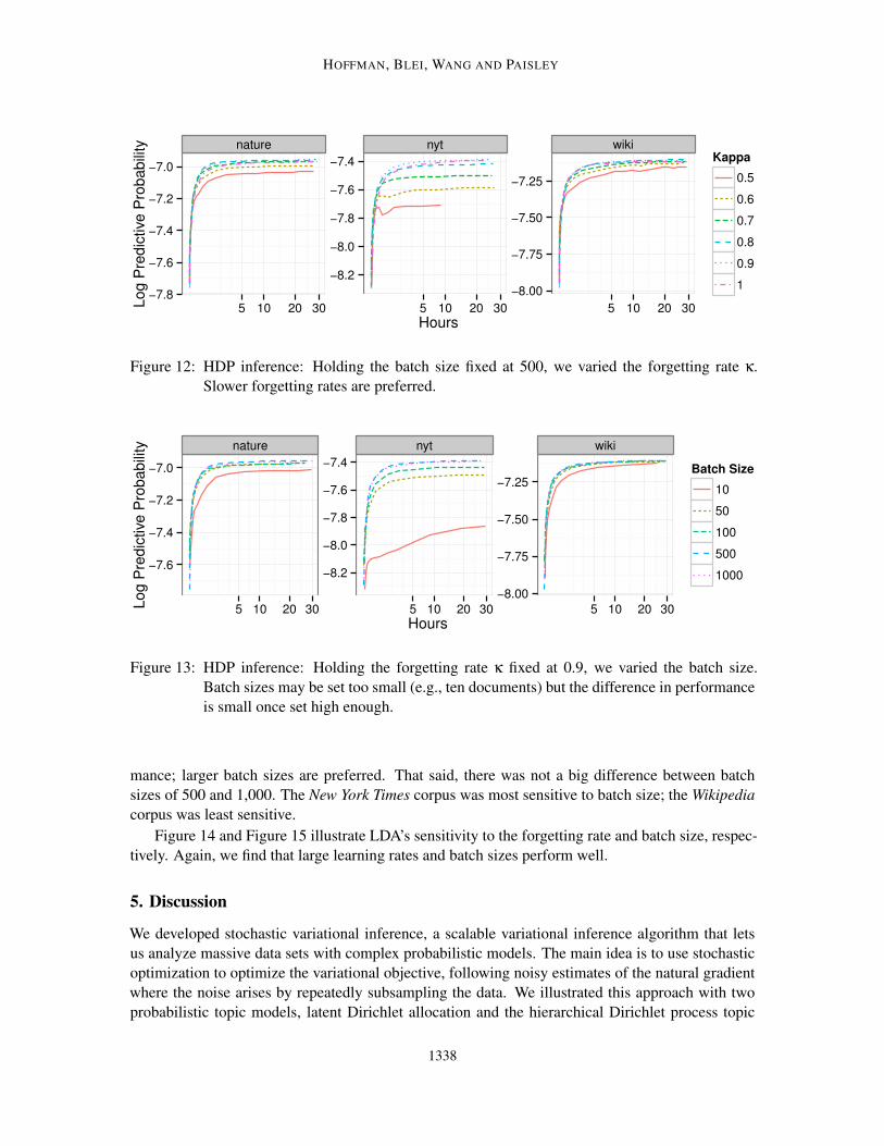
HOFFMAN, BLEI, WANG AND PAISLEY
nature nyt wiki
−7.8
−7.6
−7.4
−7.2
−7.0
−8.2
−8.0
−7.8
−7.6
−7.4
−8.00
−7.75
−7.50
−7.25
5 10 20 30 5 10 20 30 5 10 20 30
Hours
Log P
redic
tive P
robabili
tyKappa
0.5
0.6
0.7
0.8
0.9
1
Figure 12: HDP inference: Holding the batch size fixed at 500, we varied the forgetting rate κ.
Slower forgetting rates are preferred.
nature nyt wiki
−7.6
−7.4
−7.2
−7.0
−8.2
−8.0
−7.8
−7.6
−7.4
−8.00
−7.75
−7.50
−7.25
5 10 20 30 5 10 20 30 5 10 20 30
Hours
Log P
redic
tive P
robabili
ty
Batch Size
10
50
100
500
1000
Figure 13: HDP inference: Holding the forgetting rate κ fixed at 0.9, we varied the batch size.
Batch sizes may be set too small (e.g., ten documents) but the difference in performance
is small once set high enough.
mance; larger batch sizes are preferred. That said, there was not a big difference between batch
sizes of 500 and 1,000. The New York Times corpus was most sensitive to batch size; the Wikipedia
corpus was least sensitive.
Figure 14 and Figure 15 illustrate LDA’s sensitivity to the forgetting rate and batch size, respec-
tively. Again, we find that large learning rates and batch sizes perform well.
5. Discussion
We developed stochastic variational inference, a scalable variational inference algorithm that lets
us analyze massive data sets with complex probabilistic models. The main idea is to use stochastic
optimization to optimize the variational objective, following noisy estimates of the natural gradient
where the noise arises by repeatedly subsampling the data. We illustrated this approach with two
probabilistic topic models, latent Dirichlet allocation and the hierarchical Dirichlet process topic
1338
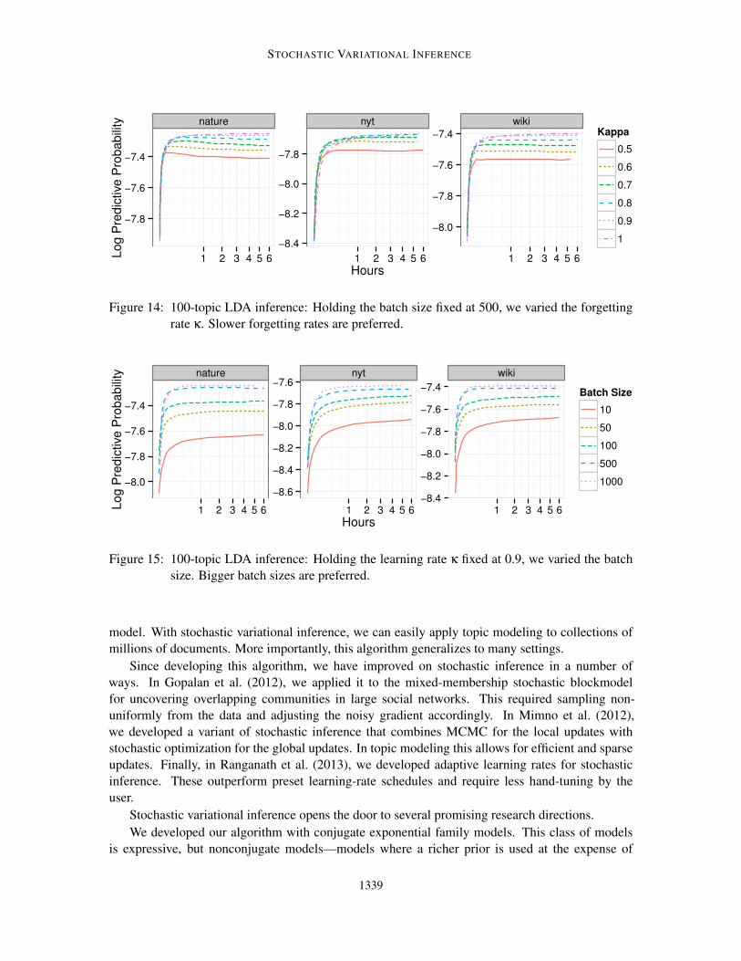
STOCHASTIC VARIATIONAL INFERENCE
nature nyt wiki
−7.8
−7.6
−7.4
−8.4
−8.2
−8.0
−7.8
−8.0
−7.8
−7.6
−7.4
1 2 3 4 5 6 1 2 3 4 5 6 1 2 3 4 5 6
Hours
Log P
redic
tive P
robabili
tyKappa
0.5
0.6
0.7
0.8
0.9
1
Figure 14: 100-topic LDA inference: Holding the batch size fixed at 500, we varied the forgetting
rate κ. Slower forgetting rates are preferred.
nature nyt wiki
−8.0
−7.8
−7.6
−7.4
−8.6
−8.4
−8.2
−8.0
−7.8
−7.6
−8.4
−8.2
−8.0
−7.8
−7.6
−7.4
1 2 3 4 5 6 1 2 3 4 5 6 1 2 3 4 5 6
Hours
Log P
redic
tive P
robabili
ty
Batch Size
10
50
100
500
1000
Figure 15: 100-topic LDA inference: Holding the learning rate κ fixed at 0.9, we varied the batch
size. Bigger batch sizes are preferred.
model. With stochastic variational inference, we can easily apply topic modeling to collections of
millions of documents. More importantly, this algorithm generalizes to many settings.
Since developing this algorithm, we have improved on stochastic inference in a number of
ways. In Gopalan et al. (2012), we applied it to the mixed-membership stochastic blockmodel
for uncovering overlapping communities in large social networks. This required sampling non-
uniformly from the data and adjusting the noisy gradient accordingly. In Mimno et al. (2012),
we developed a variant of stochastic inference that combines MCMC for the local updates with
stochastic optimization for the global updates. In topic modeling this allows for efficient and sparse
updates. Finally, in Ranganath et al. (2013), we developed adaptive learning rates for stochastic
inference. These outperform preset learning-rate schedules and require less hand-tuning by the
user.
Stochastic variational inference opens the door to several promising research directions.
We developed our algorithm with conjugate exponential family models. This class of models
is expressive, but nonconjugate models—models where a richer prior is used at the expense of
1339
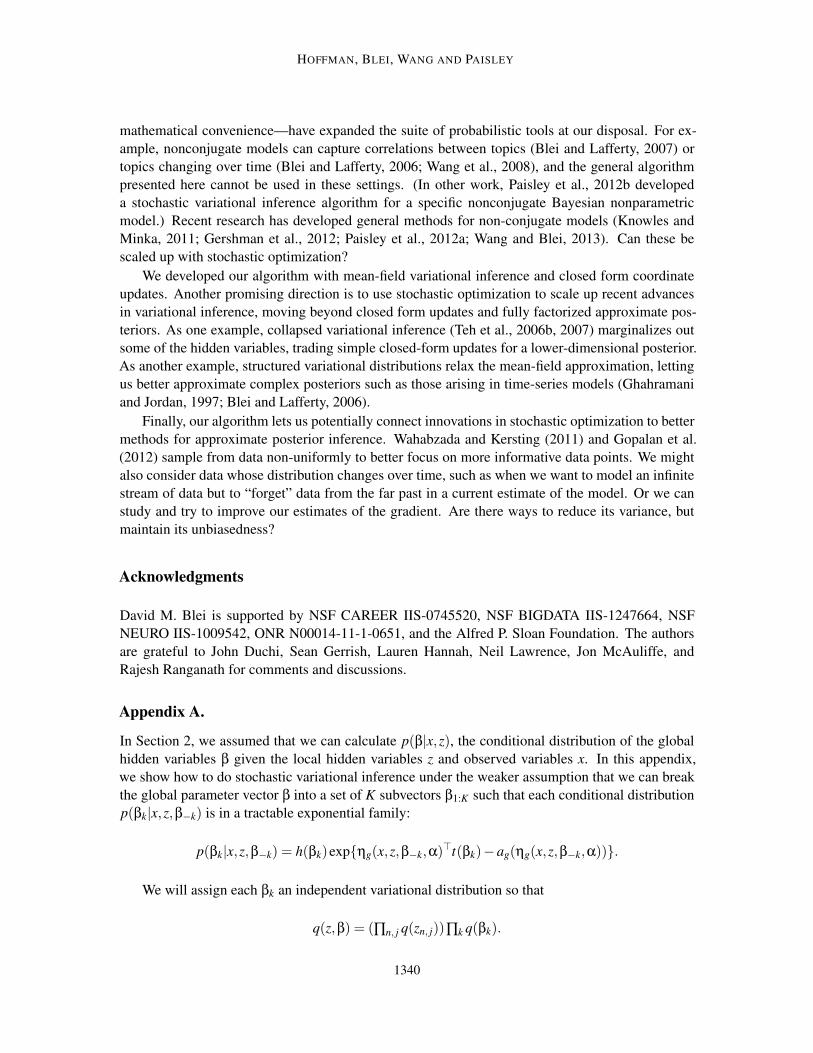
HOFFMAN, BLEI, WANG AND PAISLEY
mathematical convenience—have expanded the suite of probabilistic tools at our disposal. For ex-
ample, nonconjugate models can capture correlations between topics (Blei and Lafferty, 2007) or
topics changing over time (Blei and Lafferty, 2006; Wang et al., 2008), and the general algorithm
presented here cannot be used in these settings. (In other work, Paisley et al., 2012b developed
a stochastic variational inference algorithm for a specific nonconjugate Bayesian nonparametric
model.) Recent research has developed general methods for non-conjugate models (Knowles and
Minka, 2011; Gershman et al., 2012; Paisley et al., 2012a; Wang and Blei, 2013). Can these be
scaled up with stochastic optimization?
We developed our algorithm with mean-field variational inference and closed form coordinate
updates. Another promising direction is to use stochastic optimization to scale up recent advances
in variational inference, moving beyond closed form updates and fully factorized approximate pos-
teriors. As one example, collapsed variational inference (Teh et al., 2006b, 2007) marginalizes out
some of the hidden variables, trading simple closed-form updates for a lower-dimensional posterior.
As another example, structured variational distributions relax the mean-field approximation, letting
us better approximate complex posteriors such as those arising in time-series models (Ghahramani
and Jordan, 1997; Blei and Lafferty, 2006).
Finally, our algorithm lets us potentially connect innovations in stochastic optimization to better
methods for approximate posterior inference. Wahabzada and Kersting (2011) and Gopalan et al.
(2012) sample from data non-uniformly to better focus on more informative data points. We might
also consider data whose distribution changes over time, such as when we want to model an infinite
stream of data but to “forget” data from the far past in a current estimate of the model. Or we can
study and try to improve our estimates of the gradient. Are there ways to reduce its variance, but
maintain its unbiasedness?
Acknowledgments
David M. Blei is supported by NSF CAREER IIS-0745520, NSF BIGDATA IIS-1247664, NSF
NEURO IIS-1009542, ONR N00014-11-1-0651, and the Alfred P. Sloan Foundation. The authors
are grateful to John Duchi, Sean Gerrish, Lauren Hannah, Neil Lawrence, Jon McAuliffe, and
Rajesh Ranganath for comments and discussions.
Appendix A.
In Section 2, we assumed that we can calculate p(β|x,z), the conditional distribution of the global
hidden variables β given the local hidden variables z and observed variables x. In this appendix,
we show how to do stochastic variational inference under the weaker assumption that we can break
the global parameter vector β into a set of K subvectors β1:K such that each conditional distribution
p(βk|x,z,β−k) is in a tractable exponential family:
p(βk|x,z,β−k) = h(βk)exp{ηg(x,z,β−k,α)⊤t(βk)−ag(ηg(x,z,β−k,α))}.
We will assign each βk an independent variational distribution so that
q(z,β) = (∏n, j q(zn, j))∏k q(βk).
1340
STOCHASTIC VARIATIONAL INFERENCE
We choose each q(βk) to be in the same exponential family as the complete conditional p(βk|x,z,β−k),
q(βk) = h(βk)exp{λ⊤k t(βk)−ag(λk)}.
We overload h(·), t(·), and a(·) so that, for example, q(βk)= p(βk|x,z,β−k) when λk =ηg(x,z,β−k,α).The natural parameter ηg(x,z,β−k,α) decomposes into two terms,
ηg(x,z,β−k,α) = ηg(β−k,α)+∑n
ηg(xn,zn,β−k,α).
The first depends only on the global parameters β−k and the hyperparameters α; the second is a sum
of N terms that depend on β−k, α, and a single local context (xn,zn).Proceeding as in Section 2, we will derive the natural gradient of the ELBO implied by this
model and choice of variational distribution. Focusing on a particular βk, we can write the ELBO as
L = Eq[log p(βk|x,z,β−k)]−Eq[logq(βk)]+ const.
= (Eq[ηg(x,z,β−k,α)]−λk)⊤∇λk
ag(λk)+ag(λk)+ const.
The gradient of L with respect to λk is then
∇λkL = ∇2
λkag(λk)(Eq[ηg(x,z,β−k,α)]−λk),
and the natural gradient of L with respect to λk is
∇λkL = Eq[ηg(x,z,β−k,α)]−λk
=−λk +Eq[ηg(β−k,α)]+∑n
Eq[ηg(xn,zn,β−k,α)].
Randomly sampling a local context (xi,zi) yields a noisy (but unbiased) estimate of the natural
gradient,
∇λkLi =−λk +Eq[ηg(β−k,α)]+NEq[ηg(xi,zi,β−k,α)]≡−λk + λk.
We can use this noisy natural gradient exactly as in Section 2. For each update t, we sample a context
(xt ,zt), optimize the local variational parameters φt by repeatedly applying equation Equation 16,
and take a step of size ρt = (t + τ)−κ in the direction of the noisy natural gradient:
λ(t)k = (1−ρt)λ
(t−1)k +ρt λk (34)
Note that the update in Equation 34 depends only on λ(t−1); we compute all elements of λ(t) simul-
taneously, whereas in a batch coordinate ascent algorithm λ(t)k could depend on λ
(t)1:k−1.
References
A. Ahmed, M. Aly, J. Gonzalez, S. Narayanamurthy, and A. Smola. Scalable inference in latent
variable models. In Web Search and Data Mining, New York, NY, USA, 2012.
S. Amari. Differential geometry of curved exponential families-curvatures and information loss.
The Annals of Statistics, 10(2):357–385, 1982.
1341
HOFFMAN, BLEI, WANG AND PAISLEY
S. Amari. Natural gradient works efficiently in learning. Neural computation, 10(2):251–276, 1998.
C. Antoniak. Mixtures of Dirichlet processes with applications to Bayesian nonparametric problems.
The Annals of Statistics, 2(6):1152–1174, 1974.
A. Asuncion, M. Welling, P. Smyth, and Y. Teh. On smoothing and inference for topic models. In
Uncertainty in Artificial Intelligence, 2009.
H. Attias. Inferring parameters and structure of latent variable models by variational bayes. In
Uncertainty in Artificial Intelligence, 1999.
H. Attias. A variational Bayesian framework for graphical models. In Neural Information Process-
ing Systems, 2000.
J. Bernardo and A. Smith. Bayesian Theory. John Wiley & Sons Ltd., Chichester, 1994.
C. Bishop. Pattern Recognition and Machine Learning. Springer New York., 2006.
C. Bishop, D. Spiegelhalter, and J. Winn. VIBES: A variational inference engine for Bayesian
networks. In Neural Information Processing Systems. Cambridge, MA, 2003.
D. Blackwell and J. MacQueen. Ferguson distributions via Pólya urn schemes. The Annals of
Statistics, 1(2):353–355, 1973.
D. Blei. Probabilistic topic models. Communications of the ACM, 55(4):77–84, 2012.
D. Blei and M. Jordan. Variational inference for Dirichlet process mixtures. Journal of Bayesian
Analysis, 1(1):121–144, 2006.
D. Blei and J. Lafferty. Dynamic topic models. In International Conference on Machine Learning,
pages 113–120, 2006.
D. Blei and J. Lafferty. A correlated topic model of Science. Annals of Applied Statistics, 1(1):
17–35, 2007.
D. Blei, A. Ng, and M. Jordan. Latent Dirichlet allocation. Journal of Machine Learning Research,
3:993–1022, January 2003.
L. Bottou. On-line learning and stochastic approximations. In On-line Learning in Neural Networks,
pages 9–42. Cambridge University Press, 1998.
L. Bottou. Stochastic learning. In Advanced Lectures on Machine Learning, pages 146–168.
Springer, 2003.
L. Bottou and O. Bousquet. Learning using large datasets. In Mining Massive Datasets for Security.
IOS Press, 2008.
Olivier Cappé and Eric Moulines. On-line expectation-maximization algorithm for latent data mod-
els. Journal of the Royal Statistical Society: Series B (Statistical Methodology), 71(3):593–613,
2009.
1342
STOCHASTIC VARIATIONAL INFERENCE
M. Collins, S. Dasgupta, and R. Schapire. A generalization of principal component analysis to the
exponential family. In Neural Information Processing Systems, 2002.
A. Dempster, N. Laird, and D. Rubin. Maximum likelihood from incomplete data via the EM
algorithm. Journal of the Royal Statistical Society, Series B, 39:1–38, 1977.
M. Do Carmo. Riemannian Geometry. Birkhäuser, 1992.
A. Doucet, N. De Freitas, and N. Gordon. An introduction to sequential Monte Carlo methods.
Springer, 2001.
E. Erosheva. Bayesian estimation of the grade of membership model. Bayesian Statistics, 7:501–
510, 2003.
M. Escobar and M. West. Bayesian density estimation and inference using mixtures. Journal of the
American Statistical Association, 90:577–588, 1995.
T. Ferguson. A Bayesian analysis of some nonparametric problems. The Annals of Statistics, 1:
209–230, 1973.
S. Fine, Y. Singer, and N. Tishby. The hierarchical hidden Markov model: Analysis and applications.
Machine Learning, 32:41–62, 1998.
E. Fox, E. Sudderth, M. Jordan, and A. Willsky. An HDP-HMM for systems with state persistence.
In International Conference on Machine Learning, 2008.
E. Fox, E. Sudderth, M. Jordan, and A. Willsky. Bayesian nonparametric inference of switching
dynamic linear models. IEEE Transactions on Signal Processing, 59(4):1569–1585, 2011a.
E. Fox, E. Sudderth, M. Jordan, and A. Willsky. A sticky HDP-HMM with application to speaker
diarization. Annals of Applied Statistics, 5(2A):1020–1056, 2011b.
S. Geisser. The predictive sample reuse method with applications. Journal of the American Statisti-
cal Association, 70:320–328, 1975.
A. Gelfand and A. Smith. Sampling based approaches to calculating marginal densities. Journal of
the American Statistical Association, 85:398–409, 1990.
A. Gelman and J. Hill. Data Analysis Using Regression and Multilevel/Hierarchical Models. Cam-
bridge University Press, 2007.
S. Geman and D. Geman. Stochastic relaxation, Gibbs distributions and the Bayesian restoration of
images. IEEE Transactions on Pattern Analysis and Machine Intelligence, 6:721–741, 1984.
S. Gershman and D. Blei. A tutorial on Bayesian nonparametric models. Journal of Mathematical
Psychology, 56:1–12, 2012.
S. Gershman, M. Hoffman, and D. Blei. Nonparametric variational inference. In International
Conference on Machine Learning, 2012.
Z. Ghahramani and M. Beal. Variational inference for Bayesian mixtures of factor analysers. In
Neural Information Processing Systems, 2000.
1343
HOFFMAN, BLEI, WANG AND PAISLEY
Z. Ghahramani and M. Beal. Propagation algorithms for variational Bayesian learning. In Neural
Information Processing Systems, pages 507–513, 2001.
Z. Ghahramani and M. Jordan. Factorial hidden Markov models. Machine Learning, 31(1), 1997.
M. Girolami and S. Rogers. Variational Bayesian multinomial probit regression with Gaussian
process priors. Neural Computation, 18(8), 2006.
P. Gopalan, D. Mimno, S. Gerrish, M. Freedman, and D. Blei. Scalable inference of overlapping
communities. In Neural Information Processing Systems, 2012.
T. Griffiths and M. Steyvers. Finding scientific topics. Proceedings of the National Academy of
Science, 101:5228–5235, 2004.
W. Hastings. Monte Carlo sampling methods using Markov chains and their applications.
Biometrika, 57:97–109, 1970.
G. Hinton and D. Van Camp. Keeping the neural networks simple by minimizing the description
length of the weights. In Computational Learning Theory, pages 5–13. ACM, 1993.
N. Hjort, C. Holmes, P. Muller, and S. Walker, editors. Bayesian Nonparametrics. Cambridge
University Press, 2010.
M. Hoffman, D. Blei, and F. Bach. On-line learning for latent Dirichlet allocation. In Neural
Information Processing Systems, 2010a.
M. Hoffman, D. Blei, and P. Cook. Bayesian nonparametric matrix factorization for recorded music.
In International Conference on Machine Learning, 2010b.
A. Honkela, M. Tornio, T. Raiko, and J. Karhunen. Natural conjugate gradient in variational infer-
ence. In Neural Information Processing Systems, 2008.
T. Jaakkola. Variational Methods for Inference and Estimation in Graphical Models. PhD thesis,
Massachusetts Institute of Technology, 1997.
M. Jordan, editor. Learning in Graphical Models. MIT Press, Cambridge, MA, 1999.
M. Jordan, Z. Ghahramani, T. Jaakkola, and L. Saul. Introduction to variational methods for graph-
ical models. Machine Learning, 37:183–233, 1999.
R. Kalman. A new approach to linear filtering and prediction problems a new approach to linear
filtering and prediction problems,”. Transaction of the AMSE: Journal of Basic Engineering, 82:
35–45, 1960.
D. Knowles and T. Minka. Non-conjugate variational message passing for multinomial and binary
regression. In Neural Information Processing Systems, 2011.
D. Koller and N. Friedman. Probabilistic Graphical Models: Principles and Techniques. The MIT
Press, 2009.
S. Kullback and R.A. Leibler. On information and sufficiency. The Annals of Mathematical Statis-
tics, 22(1):79–86, 1951.
1344
STOCHASTIC VARIATIONAL INFERENCE
P. Liang, M. Jordan, and D. Klein. Learning semantic correspondences with less supervision. In
Association of Computational Linguisitics, 2009.
J. Mairal, J. Bach, J. Ponce, and G. Sapiro. Online learning for matrix factorization and sparse
coding. Journal of Machine Learning Research, 11:19–60, 2010.
J. Maritz and T. Lwin. Empirical Bayes Methods. Monographs on Statistics and Applied Probability.
Chapman & Hall, London, 1989.
P. McCullagh and J. A. Nelder. Generalized Linear Models. London: Chapman and Hall, 1989.
N. Metropolis, A. Rosenbluth, M. Rosenbluth, M. Teller, and E. Teller. Equations of state calcula-
tions by fast computing machines. Journal of Chemical Physics, 21:1087–1092, 1953.
D. Mimno, M. Hoffman, and D. Blei. Sparse stochastic inference for latent Dirichlet allocation. In
International Conference on Machine Learning, 2012.
T. Minka and J. Lafferty. Expectation-propagation for the generative aspect model. In Uncertainty
in Artificial Intelligence (UAI), 2002.
K. Murphy. Machine Learning: A Probabilistic Approach. MIT Press, 2012.
R. Neal. Markov chain sampling methods for Dirichlet process mixture models. Journal of Compu-
tational and Graphical Statistics, 9(2):249–265, 2000.
R. Neal and G. Hinton. A view of the EM algorithm that justifies incremental, sparse, and other
variants. In Learning in graphical models, pages 355–368. MIT Press, 1999.
D. Newman, A. Asuncion, P. Smyth, and M. Welling. Distributed algorithms for topic models.
Journal of Machine Learning Research, 10:1801–1828, 2009.
J. Paisley and L. Carin. Nonparametric factor analysis with beta process priors. In International
Conference on Machine Learning, 2009.
J. Paisley, D. Blei, and M. Jordan. Variational Bayesian inference with stochastic search. In Inter-
national Conference on Machine Learning, 2012a.
J. Paisley, C. Wang, and D. Blei. The discrete infinite logistic normal distribution. Bayesian Analysis,
7(2):235–272, 2012b.
J. Paisley, C. Wang, D. Blei, and M. Jordan. Nested hierarchical Dirichlet processes. arXiv preprint
arXiv:1210.6738, 2012c.
G. Parisi. Statistical Field Theory. Perseus Books, 1988.
J. Pearl. Probabilistic Reasoning in Intelligent Systems: Networks of Plausible Inference. Morgan
Kaufmann, 1988. ISBN 1558604790.
C. Peterson and J. Anderson. A mean field theory learning algorithm for neural networks. Complex
Systems, 1(5):995–1019, 1987.
1345
HOFFMAN, BLEI, WANG AND PAISLEY
J. Pitman. Combinatorial Stochastic Processes. Lecture Notes for St. Flour Summer School.
Springer-Verlag, New York, NY, 2002.
J. Platt, E. Kıcıman, and D. Maltz. Fast variational inference for large-scale internet diagnosis.
Neural Information Processing Systems, 2008.
L. Rabiner. A tutorial on hidden Markov models and selected applications in speech recognition.
Proceedings of the IEEE, 77:257–286, 1989.
R. Ranganath, C. Wang, D. Blei, and E. Xing. An adaptive learning rate for stochastic variational
inference. In International Conference on Machine Learning, 2013.
H. Robbins and S. Monro. A stochastic approximation method. The Annals of Mathematical Statis-
tics, 22(3):400–407, 1951.
C. Robert and G. Casella. Monte Carlo Statistical Methods. Springer Texts in Statistics. Springer-
Verlag, New York, NY, 2004.
R. Salakhutdinov and A. Mnih. Bayesian probabilistic matrix factorization using Markov chain
Monte Carlo. In International Conference on Machine learning, pages 880–887, 2008.
M. Sato. Online model selection based on the variational Bayes. Neural Computation, 13(7):1649–
1681, 2001.
L. Saul and M. Jordan. Exploiting tractable substructures in intractable networks. Neural Informa-
tion Processing Systems, 1996.
L. Saul, T. Jaakkola, and M. Jordan. Mean field theory for sigmoid belief networks. Journal of
Artificial Intelligence Research, 4:61–76, 1996.
J. Sethuraman. A constructive definition of Dirichlet priors. Statistica Sinica, 4:639–650, 1994.
A. Smola and S. Narayanamurthy. An architecture for parallel topic models. In Very Large
Databases, 2010.
J. Spall. Introduction to Stochastic Search and Optimization: Estimation, Simulation, and Control.
John Wiley and Sons, 2003.
C. Spearman. "General intelligence," objectively determined and measured. The American Journal
of Psychology, pages 201–292, 1904.
Y. Teh, M. Jordan, M. Beal, and D. Blei. Hierarchical Dirichlet processes. Journal of the American
Statistical Association, 101(476):1566–1581, 2006a.
Y. Teh, D. Newman, and M. Welling. A collapsed variational Bayesian inference algorithm for
latent Dirichlet allocation. In Neural Information Processing Systems, 2006b.
Y. Teh, K. Kurihara, and M. Welling. Collapsed variational inference for HDP. In Neural Informa-
tion Processing Systems, 2007.
M. Tipping and C. Bishop. Probabilistic principal component analysis. Journal of the Royal Statis-
tical Society: Series B (Statistical Methodology), 61(3):611–622, 1999.
1346
STOCHASTIC VARIATIONAL INFERENCE
M. Wahabzada and K. Kersting. Larger residuals, less work: Active document scheduling for latent
dirichlet allocation. In European Conference on Machine Learning, 2011.
M. Wainwright and M. Jordan. Graphical models, exponential families, and variational inference.
Foundations and Trends in Machine Learning, 1(1–2):1–305, 2008.
H. Wallach, D. Mimno, and A. McCallum. Rethinking LDA: Why priors matter. In Neural Infor-
mation Processing Systems. 2009.
C. Wang. Variational Bayesian approach to canonical correlation analysis. IEEE Transactions on
Neural Networks, 2006.
C. Wang and D. Blei. Variational inference in nonconjugate models. Journal of Machine Learning
Research, 2013.
C. Wang, D. Blei, and D. Heckerman. Continuous time dynamic topic models. In Uncertainty in
Artificial Intelligence, 2008.
C. Wang, J. Paisley, and D. Blei. Online variational inference for the hierarchical Dirichlet process.
In Artificial Intelligence and Statistics, 2011.
S. Waterhouse, D. MacKay, and T. Robinson. Bayesian methods for mixtures of experts. Neural
Information Processing Systems, pages 351–357, 1996.
M. Welling and Y. Teh. Bayesian learning via stochastic gradient Langevin dynamics. In Interna-
tional Conference on Machine Learning, 2011.
W. Wiegerinck. Variational approximations between mean field theory and the junction tree algo-
rithm. In Uncertainty in Artificial Intelligence, 2000.
E. Xing, M. Jordan, and S. Russell. A generalized mean field algorithm for variational inference in
exponential families. In Uncertainty in Artificial Intelligence, 2003.
1347