Towards Verified Stochastic Variational Inference for ...
34
HAL Id: hal-02399922 https://hal.archives-ouvertes.fr/hal-02399922 Submitted on 9 Dec 2019 HAL is a multi-disciplinary open access archive for the deposit and dissemination of sci- entific research documents, whether they are pub- lished or not. The documents may come from teaching and research institutions in France or abroad, or from public or private research centers. L’archive ouverte pluridisciplinaire HAL, est destinée au dépôt et à la diffusion de documents scientifiques de niveau recherche, publiés ou non, émanant des établissements d’enseignement et de recherche français ou étrangers, des laboratoires publics ou privés. Towards Verified Stochastic Variational Inference for Probabilistic Programs Wonyeol Lee, Hangyeol Yu, Xavier Rival, Hongseok Yang To cite this version: Wonyeol Lee, Hangyeol Yu, Xavier Rival, Hongseok Yang. Towards Verified Stochastic Variational Inference for Probabilistic Programs. Proceedings of the ACM on Programming Languages, ACM, In press, 16, 10.1145/3371084. hal-02399922
Transcript of Towards Verified Stochastic Variational Inference for ...
HAL Id: hal-02399922https://hal.archives-ouvertes.fr/hal-02399922
Submitted on 9 Dec 2019
HAL is a multi-disciplinary open accessarchive for the deposit and dissemination of sci-entific research documents, whether they are pub-lished or not. The documents may come fromteaching and research institutions in France orabroad, or from public or private research centers.
L’archive ouverte pluridisciplinaire HAL, estdestinée au dépôt et à la diffusion de documentsscientifiques de niveau recherche, publiés ou non,émanant des établissements d’enseignement et derecherche français ou étrangers, des laboratoirespublics ou privés.
Towards Verified Stochastic Variational Inference forProbabilistic Programs
Wonyeol Lee, Hangyeol Yu, Xavier Rival, Hongseok Yang
To cite this version:Wonyeol Lee, Hangyeol Yu, Xavier Rival, Hongseok Yang. Towards Verified Stochastic VariationalInference for Probabilistic Programs. Proceedings of the ACM on Programming Languages, ACM, Inpress, 16, �10.1145/3371084�. �hal-02399922�
16
Towards Verified Stochastic Variational Inference forProbabilistic Programs
WONYEOL LEE, School of Computing, KAIST, South Korea
HANGYEOL YU, School of Computing, KAIST, South Korea
XAVIER RIVAL, INRIA Paris, CNRS/École Normale Supérieure/PSL University, France
HONGSEOK YANG, School of Computing, KAIST, South Korea
Probabilistic programming is the idea of writing models from statistics and machine learning using program
notations and reasoning about these models using generic inference engines. Recently its combination with
deep learning has been explored intensely, which led to the development of so called deep probabilistic
programming languages, such as Pyro, Edward and ProbTorch. At the core of this development lie inference
engines based on stochastic variational inference algorithms. When asked to find information about the
posterior distribution of a model written in such a language, these algorithms convert this posterior-inference
query into an optimisation problem and solve it approximately by a form of gradient ascent or descent. In
this paper, we analyse one of the most fundamental and versatile variational inference algorithms, called
score estimator or REINFORCE, using tools from denotational semantics and program analysis. We formally
express what this algorithm does on models denoted by programs, and expose implicit assumptions made
by the algorithm on the models. The violation of these assumptions may lead to an undefined optimisation
objective or the loss of convergence guarantee of the optimisation process. We then describe rules for proving
these assumptions, which can be automated by static program analyses. Some of our rules use nontrivial
facts from continuous mathematics, and let us replace requirements about integrals in the assumptions, such
as integrability of functions defined in terms of programs’ denotations, by conditions involving differentia-
tion or boundedness, which are much easier to prove automatically (and manually). Following our general
methodology, we have developed a static program analysis for the Pyro programming language that aims at
discharging the assumption about what we call model-guide support match. Our analysis is applied to the
eight representative model-guide pairs from the Pyro webpage, which include sophisticated neural network
models such as AIR. It finds a bug in one of these cases, reveals a non-standard use of an inference engine in
another, and shows that the assumptions are met in the remaining six cases.
CCS Concepts: •Mathematics of computing→Bayesian computation;Variationalmethods; •Theoryof computation→ Probabilistic computation;Denotational semantics; • Software and its engineer-ing → Correctness; Automated static analysis; • Computing methodologies→ Machine learning.
Additional Key Words and Phrases: Probabilistic programming, static analysis, semantics, correctness
ACM Reference Format:Wonyeol Lee, Hangyeol Yu, Xavier Rival, and Hongseok Yang. 2020. Towards Verified Stochastic Variational
Inference for Probabilistic Programs. Proc. ACM Program. Lang. 4, POPL, Article 16 (January 2020), 33 pages.
https://doi.org/10.1145/3371084
Authors’ addresses: Wonyeol Lee, School of Computing, KAIST, South Korea, [email protected]; Hangyeol Yu, School of
Computing, KAIST, South Korea, [email protected]; Xavier Rival, INRIA Paris, CNRS/École Normale Supérieure/PSL
University, France, [email protected]; Hongseok Yang, School of Computing, KAIST, South Korea, [email protected].
Permission to make digital or hard copies of part or all of this work for personal or classroom use is granted without fee
provided that copies are not made or distributed for profit or commercial advantage and that copies bear this notice and
the full citation on the first page. Copyrights for third-party components of this work must be honored. For all other uses,
contact the owner/author(s).
© 2020 Copyright held by the owner/author(s).
2475-1421/2020/1-ART16
https://doi.org/10.1145/3371084
Proc. ACM Program. Lang., Vol. 4, No. POPL, Article 16. Publication date: January 2020.
16:2 Wonyeol Lee, Hangyeol Yu, Xavier Rival, and Hongseok Yang
1 INTRODUCTIONProbabilistic programming refers to the idea of writing models from statistics and machine learning
using program notations and reasoning about these models using generic inference engines. It has
been the subject of active research in machine learning and programming languages, because of its
potential for enabling scientists and engineers to design and explore sophisticated models easily;
when using these languages, they no longer have to worry about developing custom inference
engines for their models, a highly-nontrivial task requiring expertise in statistics and machine
learning. Several practical probabilistic programming languages now exist, and are used for a wide
range of applications [Carpenter et al. 2017; Gehr et al. 2016; Goodman et al. 2008; Gordon et al.
2014; Mansinghka et al. 2014; Minka et al. 2014; Narayanan et al. 2016; Wood et al. 2014].
We consider inference engines that lie at the core of so called deep probabilistic programming
languages, such as Pyro [Bingham et al. 2019], Edward [Tran et al. 2018, 2016] and ProbTorch
[Siddharth et al. 2017]. These languages let users freely mix deep neural networks with constructs
from probabilistic programming, in particular, those for writing Bayesian probabilistic models. In
so doing, they facilitate the development of probabilistic deep-network models that may address
the problem of measuring the uncertainty in current non-Bayesian deep-network models; a non-
Bayesian model may predict that the price of energy goes up and that of a house goes down, but it
cannot express, for instance, that the model is confident with the first prediction but not the second.
The primary inference engines for these deep probabilistic programming languages implement
stochastic (or black-box) variational inference1algorithms. Converting inference problems into
optimisation problems is the high-level idea of these algorithms.2When asked to find information
about the posterior distribution of a model written in such a language, these algorithms convert
this question to an optimisation problem and solve the problem approximately by performing
a gradient descent or ascent on the optimisation objective. The algorithms work smoothly with
gradient-based parameter-learning algorithms for deep neural networks, which is why they form
the backbone for deep probabilistic programming languages.
In this paper, we analyse one of the most fundamental and versatile variational inference algo-
rithms, called score estimator or REINFORCE3[Paisley et al. 2012; Ranganath et al. 2014; Williams
1992; Wingate and Weber 2013], using tools from denotational semantics and program analy-
sis [Cousot and Cousot 1977, 1979, 1992]. We formally express what this algorithm does on models
denoted by probabilistic programs, and expose implicit assumptions made by the algorithm on
the models. The violation of these assumptions can lead to undefined optimisation objective or
the loss of convergence guarantee of the optimisation process. We then describe rules for proving
these assumptions, which can be automated by static program analyses. Some of our rules use
nontrivial facts from continuous mathematics, and let us replace requirements about integrals in the
assumptions, such as integrability of functions defined in terms of programs’ denotations, by the
conditions involving differentiation or boundedness, which are much easier to prove automatically
(and manually) than the original requirements.
Following our general methodology, we have developed a static program analysis for the Pyro
programming language that can discharge one assumption of the inference algorithm about so
1The term stochastic variational inference (VI) often refers to VI with data subsampling [Hoffman et al. 2013], and our usage
of the term is often called black-box VI [Ranganath et al. 2014] to stress the treatment of a model as a black-box sampler.
2The inference problems in their original forms involve solving summation/integration/counting problems, which are
typically more difficult than optimisation problems. The variational-inference algorithms convert the former problems to
the latter ones, by looking for approximate, not exact, answers to the former.
3REINFORCE [Williams 1992] is an algorithm originally developed for reinforcement learning (RL), but it is commonly used
as a synonym of the score-estimator algorithm. This is because REINFORCE and score estimator use a nearly identical
method for estimating the gradient of an optimisation objective.
Proc. ACM Program. Lang., Vol. 4, No. POPL, Article 16. Publication date: January 2020.
Towards Verified Stochastic Variational Inference for Probabilistic Programs 16:3
called model-guide pairs. In Pyro and other deep probabilistic programming languages, a program
denoting a model typically comes with a companion program, called guide, decoder, or inference
network. This companion, which we call guide, helps the inference algorithm to find a good
approximation to what the model ultimately denotes under a given dataset (i.e., the posterior
distribution of the model under the dataset); the algorithm uses the guide to fix the search space of
approximations, and solves an optimisation problem defined on that space. A model and a guide
should satisfy an important correspondence property, which says that they should use the same
sets of random variables, and for any such random variable, if the probability of the variable having
a particular value is zero in the model, it should also be zero in the guide. If the property is violated,
the inference algorithm may attempt to solve an optimisation problem with undefined optimisation
objective and return parameter values that do not make any sense. Our static analysis checks this
correspondence property for Pyro programs. When applied to eight representative model-guide
pairs from the Pyro webpage, which include sophisticated neural network models such as Attend-
Infer-Repeat (AIR), the analysis found a bug in one of these cases, revealed a non-standard use of
the inference algorithm in another, and proved that the property holds in the remaining six cases.
Another motivation for this paper is to demonstrate an opportunity for programming languages
and verification research to have an impact on the advances of machine learning and AI technologies.
One popular question is: what properties should we verify on machine-learning programs? Multiple
answers have been proposed, which led to excellent research results, such as those on robustness
of neural networks [Mirman et al. 2018]. But most of the existing research focuses on the final
outcome of machine learning algorithms, not the process of applying these algorithms. One of
our main objectives is to show that the process often relies on multiple assumptions on models
and finding automatic ways for discharging these assumptions can be another way of making PL
and verification techniques contribute. While our suggested solutions are not complete, they are
intended to show the richness of this type of problems in terms of theory and practice.
We summarise the contributions of the paper:
• We formally express the behaviour of themost fundamental variational inference algorithm on
probabilistic programs using denotational semantics, and identify requirements on program
denotations that are needed for this algorithm to work correctly.
• We describe conditions that imply the identified requirements but are easier to prove. The
sufficiency of the conditions relies on nontrivial results from continuous mathematics. We
sketch a recipe for building program analyses for checking these conditions automatically.
• Wepresent a static analysis for the Pyro language that checks the correspondence requirement
of model-guide pairs. The analysis is based on our recipe, but extends it significantly to address
challenges for dealing with features of the real-world language. Our analysis has successfully
verified 6 representative Pyro model-guide examples, and found a bug in one example.
The extended version of the paper can be found in [Lee et al. 2019].
2 VARIATIONAL INFERENCE AND VERIFICATION CHALLENGES BY EXAMPLESWe start by explaining informally the idea of stochastic variational inference (in short SVI), one
fundamental SVI algorithm, and the verification challenges that arise when we use this algorithm.
2.1 Stochastic Variational InferenceIn a probabilistic programming language, we specify a model by a program. The program model()
in Figure 1(a) is an example. It describes a joint probability density p(v, obs) on two real-valued
random variables v and obs. The value of the former is not observed, while the latter is observed
to have the value 0. Finding out the value of v is the objective of writing this model. The joint
Proc. ACM Program. Lang., Vol. 4, No. POPL, Article 16. Publication date: January 2020.
16:4 Wonyeol Lee, Hangyeol Yu, Xavier Rival, and Hongseok Yang
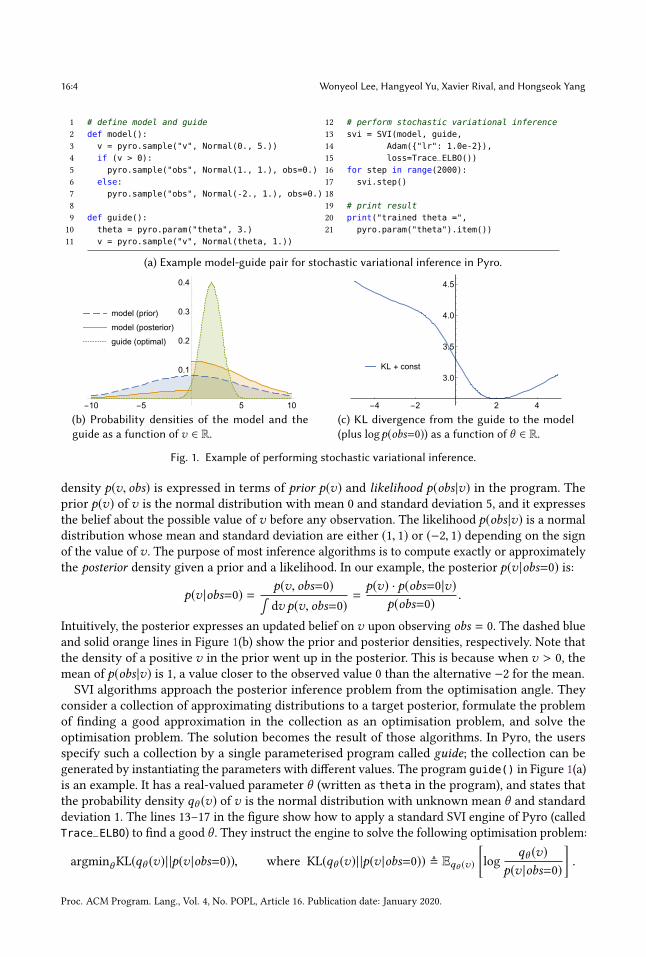
1 # define model and guide2 def model():3 v = pyro.sample("v", Normal(0., 5.))4 if (v > 0):5 pyro.sample("obs", Normal(1., 1.), obs=0.)6 else:7 pyro.sample("obs", Normal(-2., 1.), obs=0.)8
9 def guide():10 theta = pyro.param("theta", 3.)11 v = pyro.sample("v", Normal(theta, 1.))
12 # perform stochastic variational inference13 svi = SVI(model, guide,14 Adam({"lr": 1.0e-2}),15 loss=Trace_ELBO())16 for step in range(2000):17 svi.step()18
19 # print result20 print("trained theta =",21 pyro.param("theta").item())
(a) Example model-guide pair for stochastic variational inference in Pyro.
model (prior)
model (posterior)
guide (optimal)
-10 -5 5 10
0.1
0.2
0.3
0.4
(b) Probability densities of the model and theguide as a function of v ∈ R.
KL + const
-4 -2 2 4
3.0
3.5
4.0
4.5
(c) KL divergence from the guide to the model(plus logp(obs=0)) as a function of θ ∈ R.
Fig. 1. Example of performing stochastic variational inference.
density p(v, obs) is expressed in terms of prior p(v) and likelihood p(obs |v) in the program. The
prior p(v) of v is the normal distribution with mean 0 and standard deviation 5, and it expresses
the belief about the possible value of v before any observation. The likelihood p(obs |v) is a normal
distribution whose mean and standard deviation are either (1, 1) or (−2, 1) depending on the sign
of the value of v . The purpose of most inference algorithms is to compute exactly or approximately
the posterior density given a prior and a likelihood. In our example, the posterior p(v |obs=0) is:
p(v |obs=0) =p(v, obs=0)∫dv p(v, obs=0)
=p(v) · p(obs=0|v)
p(obs=0).
Intuitively, the posterior expresses an updated belief on v upon observing obs = 0. The dashed blue
and solid orange lines in Figure 1(b) show the prior and posterior densities, respectively. Note that
the density of a positive v in the prior went up in the posterior. This is because when v > 0, the
mean of p(obs |v) is 1, a value closer to the observed value 0 than the alternative −2 for the mean.
SVI algorithms approach the posterior inference problem from the optimisation angle. They
consider a collection of approximating distributions to a target posterior, formulate the problem
of finding a good approximation in the collection as an optimisation problem, and solve the
optimisation problem. The solution becomes the result of those algorithms. In Pyro, the users
specify such a collection by a single parameterised program called guide; the collection can be
generated by instantiating the parameters with different values. The program guide() in Figure 1(a)
is an example. It has a real-valued parameter θ (written as theta in the program), and states that
the probability density qθ (v) of v is the normal distribution with unknown mean θ and standard
deviation 1. The lines 13–17 in the figure show how to apply a standard SVI engine of Pyro (called
Trace_ELBO) to find a good θ . They instruct the engine to solve the following optimisation problem:
argminθKL(qθ (v)| |p(v |obs=0)), where KL(qθ (v)| |p(v |obs=0)) ≜ Eqθ (v)
[log
qθ (v)
p(v |obs=0)
].
Proc. ACM Program. Lang., Vol. 4, No. POPL, Article 16. Publication date: January 2020.

Towards Verified Stochastic Variational Inference for Probabilistic Programs 16:5
The optimisation objective KL(qθ (v)| |p(v |obs=0)) is the KL divergence from qθ (v) to p(v |obs=0),and measures the similarity between the two densities, having a small value when the densities are
similar. The KL divergence is drawn in Figure 1(c) as a function of θ , and the dotted green line in
Figure 1(b) draws the density qθ at the optimum θ . Note that the mean of this distribution is biased
toward the positive side, which reflects the fact that the property v > 0 has a higher probability
than its negation v ≤ 0 in the posterior distribution.
One of the most fundamental and versatile algorithms for SVI is score estimator (also called RE-
INFORCE). It repeatedly improves θ in two steps. First, it estimates the gradient of the optimisation
objective with samples from the current qθn :
∇θKL(qθ (v)| |p(v |obs=0))���θ=θn
≈1
N
N∑i=1
(∇θ logqθn (vi )) · logqθn (vi )
p(vi , obs=0)
where v1, . . . ,vN are independent samples from the distribution qθn . Then, the algorithm updates
θ with the estimated gradient (the specific learning rate 0.01 is chosen to improve readability):
θn+1 ← θn − 0.01 ×1
N
N∑i=1
(∇θ logqθn (vi )) · logqθn (vi )
p(vi , obs=0).
When the learning rate 0.01 is adjusted according to a known scheme, the algorithm is guaranteed
to converge to a local optimum (in many cases) because its gradient estimate satisfies the following
unbiasedness property (in those cases):
∇θKL(qθ (v)| |p(v |obs=0))���θ=θn
= E
[1
N
N∑i=1
(∇θ logqθn (vi )) · logqθn (vi )
p(vi , obs=0)
](1)
where the expectation is taken over the independent samples v1, . . . ,vN from qθn .
2.2 Verification ChallengesWe now give two example model-guide pairs that illustrate verification challenges related to SVI.
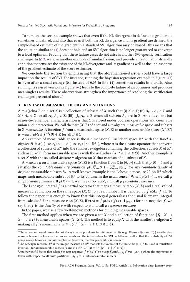
The first example appears in Figure 2(a). It is the Bayesian regression example from the Pyro
webpage (this example is among the benchmarks used in §8), which solves the problem of finding
a line that interpolates a given set of points in R2.The problem with this example is that the KL divergence of its model-guide pair, the main
optimisation objective in SVI, is undefined. The model and guide in the figure use the random
variable sigma, but they use different non-zero-probability regions, called supports, for it. In the
model, the support is [0, 10], while that in the guide is R. But the KL divergence from a guide to a
model is defined only if for every random variable, its support in the guide is included in that in the
model. We point out that this support mismatch was found by our static analyser explained in §8.
Figures 2(b) and 2(c) show two attempts to resolve the undefined-KL issue. To fix the issue, we
change the distribution of sigma in the model in (b), and in the guide in (c). These revisions remove
the problem about the support of sigma, but do not eliminate that of the undefined KL. In both (b)
and (c), the KL divergence is∞. This happens mainly because sigma can be arbitrarily close to 0 in
the guide in both cases, which makes integrand in the definition of the KL divergence diverge to∞.
An SVI-specific verification challenge related to this example is how to prove the well-definedness
of the KL divergence and more generally the optimisation objective of an SVI algorithm. In §6.2,
we provide a partial answer to the question. We give a condition for ensuring the well-definedness
of the KL divergence. Our condition is more automation-friendly than the definition of KL, because
it does not impose the difficult-to-check integrability requirement present in the definition of KL.
Proc. ACM Program. Lang., Vol. 4, No. POPL, Article 16. Publication date: January 2020.

16:6 Wonyeol Lee, Hangyeol Yu, Xavier Rival, and Hongseok Yang
1 def model(...):2 ...3 sigma = pyro.sample("sigma",
4 Uniform (0., 10.))
5 ...6 pyro.sample("obs",7 Normal(..., sigma), obs=...)
8 def guide(...):9 ...10 loc = pyro.param("sigma_loc", 1.,11 constraint=constraints.positive)12 ...13 sigma = pyro.sample("sigma",
14 Normal (loc, 0.05))
(a) Bayesian regression example from the Pyro webpage.
1 def model_r1(...):2 ...3 sigma = pyro.sample("sigma",
4 Normal (5., 5.))
5 ...6 pyro.sample("obs",7 Normal(..., abs(sigma)), obs=...)8
9 def guide_r1(...):10 # same as guide() in (a)11 ...
(b) The example with a revised model.
1 def model_r2(...):2 # same as model() in (a)3 ...4
5 def guide_r2(...):6 ...7 sigma = pyro.sample("sigma",
8 Uniform (0., 10.))
(c) The example with a revised guide.
Fig. 2. Example model-guide pairs whose KL divergence is undefined.
1 def model():2 v = pyro.sample("v", Normal(0., 5.))3 if (v > 0):4 pyro.sample("obs", Normal(1., 1.), obs=0.)5 else:6 pyro.sample("obs", Normal(-2., 1.), obs=0.)7
8 def guide():9 theta = pyro.param("theta", 3.)10 v = pyro.sample("v",
11 Uniform (theta-1., theta+1.))
(a) The model from Figure 1(a), and a guideusing a parameterised uniform distribution.
KL + const
-4 -2 0 2 4
3.5
4.0
4.5
5.0
(b) KL divergence from the guide to the model(plus logp(obs=0)) as a function of θ ∈ R.
Fig. 3. Example model-guide pair for which the gradient of the KL divergence is undefined, or the scoreestimator is biased.
The second example appears in Figure 3(a). It uses the same model as in Figure 1(a), but has a
new guide that uses a uniform distribution parameterised by θ ∈ R. For this model-guide pair, the
KL divergence is well-defined for all θ ∈ R, and the optimal θ ∗ minimising the KL is θ ∗ = 1.
However, as shown in Figure 3(b), the gradient of the KL divergence is undefined for θ ∈ {−1, 1},because the KL divergence is not differentiable at −1 and 1. For all the other θ ∈ R \ {−1, 1}, the KLdivergence and its gradient are both defined, but the score estimator cannot estimate this gradient
in an unbiased manner (i.e., in a way satisfying (1)), thereby losing the convergence guarantee to a
local optimum. The precise calculation is not appropriate in this section, but we just point out that
the expectation of the estimated gradient is always zero for all θ ∈ R \ {−1, 1}, but the true gradient
of the KL is always non-zero for those θ , because it has the form:θ25− 1[−1≤θ ≤1] ·
1
2log
N(0;1,1)N(0;−2,1) .
Here N(v; µ,σ ) is the density of the normal distribution with mean µ and standard deviation σ
(concretely,N(v ; µ,σ ) = 1/(√2πσ ) ·exp(−(v−µ)2/(2σ 2))). The mismatch comes from the invalidity
of one implicit assumption about interchanging integration and gradient in the justification of the
score estimator; see §5 for detail.
Proc. ACM Program. Lang., Vol. 4, No. POPL, Article 16. Publication date: January 2020.
Towards Verified Stochastic Variational Inference for Probabilistic Programs 16:7
To sum up, the second example shows that even if the KL divergence is defined, its gradient is
sometimes undefined, and also that even if both the KL divergence and its gradient are defined, the
sample-based estimate of the gradient in a standard SVI algorithm may be biased—this means that
the equation similar to (1) does not hold and an SVI algorithm is no longer guaranteed to converge
to a local optimum. Proving that these failure cases do not arise is another SVI-specific verification
challenge. In §6.3, we give another example of similar flavour, and provide an automation-friendly
condition that ensures the existence of the KL divergence and its gradient as well as the unbiasedness
of the gradient estimate of the score estimator.
We conclude the section by emphasising that the aforementioned issues could have a large
impact on the results of SVI. For instance, running the Bayesian regression example in Figure 2(a)
in Pyro after a small change (0.4 instead of 0.05 in line 14) sometimes results in a crash. Also,
running its revised version in Figure 2(c) leads to the complete failure of an optimiser and produces
meaningless results. These observations strengthen the importance of resolving the verification
challenges presented above.4
3 REVIEW OF MEASURE THEORY AND NOTATIONSA σ -algebra Σ on a set X is a collection of subsets of X such that (i) X ∈ Σ; (ii) A0 ∪ A1 ∈ Σ and
X \ A0 ∈ Σ for all A0,A1 ∈ Σ; (iii)⋃
n An ∈ Σ when all subsets An are in Σ. An equivalent but
easier-to-remember characterisation is that Σ is closed under boolean operations and countable
union and intersection. We call the pair (X , Σ) of a set and a σ -algebrameasurable space, and subsetsin Σ measurable. A function f from a measurable space (X , Σ) to another measurable space (X ′, Σ′)is measurable if f −1(B) ∈ Σ for all B ∈ Σ′.An example of measurable space is the n-dimensional Euclidean space Rn with the Borel σ -
algebra B ≜ σ ({(−∞, r1) × · · · × (−∞, rn)�� r ∈ Rn}), where σ is the closure operator that converts
a collection of subsets of Rn into the smallest σ -algebra containing the collection. Subsets X of Rn ,such as [0,∞)n , form measurable spaces with the σ -algebra {X ∩A | A ∈ B}. Another example is
a set X with the so called discrete σ -algebra on X that consists of all subsets of X .
A measure µ on a measurable space (X , Σ) is a function from Σ to [0,∞] such that µ(∅) = 0 and µsatisfies the countable additivity condition: µ(
⋃∞n=0 Bn) =
∑∞n=0 µ(Bn) for any countable family of
disjoint measurable subsets Bn . A well-known example is the Lebesgue measure λn on Rn which
maps each measurable subset of Rn to its volume in the usual sense.5When µ(X ) ≤ 1, we call µ
subprobability measure. If µ(X ) = 1, we may drop “sub”, and call µ probability measure.The Lebesgue integral
∫is a partial operator that maps a measure µ on (X , Σ) and a real-valued
measurable function on the same space (X , Σ) to a real number. It is denoted by
∫µ(dx) f (x). To
follow the paper, it is enough to know that this integral generalises the usual Riemann integral
from calculus.6For a measure ν on (X , Σ), if ν (A) =
∫µ(dx) (f (x) · 1[x ∈A]) for non-negative f , we
say that f is the density of ν with respect to µ and call µ reference measure.In the paper, we use a few well-known methods for building measurable spaces.
The first method applies when we are given a set X and a collection of functions { fi : X →Xi | i ∈ I } to measurable spaces (Xi , Σi ). The method is to equip X with the smallest σ -algebra Σmaking all fi ’s measurable: Σ ≜ σ ({ f −1i (B) | i ∈ I , B ∈ Σi }).
4The aforementioned issues do not always cause problems in inference results (e.g., Figures 2(a) and 2(c) mostly give
reasonable results), because the random seeds and the initial values for SVI could be set well so that the probability of SVI
going wrong becomes low. We emphasise, however, that the probability is non-zero.
5The Lebesgue measure λn is the unique measure on Rn that sets the volume of the unit cube (0, 1)n to 1 and is translation
invariant: for all measurable subsets A and r ∈ Rn , λn (A) = λn ({r ′ − r | r ′ ∈ A}).6Another useful fact is that when f is non-negative,
∫µ(dx ) f (x ) = sup
∑i (infx∈Ai f (x )) · µ(Ai ) where the supremum is
taken with respect to all finite partitions {Ai }i of X into measurable subsets.
Proc. ACM Program. Lang., Vol. 4, No. POPL, Article 16. Publication date: January 2020.

16:8 Wonyeol Lee, Hangyeol Yu, Xavier Rival, and Hongseok Yang
The second relies on two constructions for sets, i.e., product and disjoint union. Suppose that we
are given measurable spaces (Xi , Σi ) for all i ∈ I . We define a product measurable space that has∏i ∈I Xi as its underlying set and the following product σ -algebra
⊗i ∈I Σi as its σ -algebra:⊗
i ∈I
Σi ≜ σ({∏
i
Ai
��� there is a finite I0 ⊆ I such that (∀j ∈ I \ I0.Aj = X j )∧ (∀i ∈ I0.Ai ∈ Σi )}).
The construction of the product σ -algebra can be viewed as a special case of the first method where
we consider the smallest σ -algebra on∏
i ∈I Xi that makes every projection map to Xi measurable.
When the Xi are disjoint, they can be combined as disjoint union. The underlying set in this case is⋃i ∈I Xi , and the σ -algebra is⊕
i ∈I
Σi ≜ {A | A ∩ Xi ∈ Σi for all i ∈ I }.
When I = {i, j} with i , j , we denote the product measurable space by (Xi ×X j , Σi ⊗Σj ). In addition,
if Xi and X j are disjoint, we write (Xi ∪ X j , Σi ⊕ Σj ) for the disjoint-union measurable space.
The third method builds a measurable space out of measures or a certain type of measures,
such as subprobability measures. For a measurable space (X , Σ), we form a measurable space with
measures. The underlying set Mea(X ) and σ -algebra ΣMea(X ) of the space are defined by
Mea(X ) ≜ {µ | µ is a measure on (X , Σ)}, ΣMea(X ) ≜ σ({{µ | µ(A) ≤ r }
�� A ∈ Σ, r ∈ R}) .The difficult part to grasp is ΣMea(X ). Once again, a good approach for understanding it is to
realise that ΣMea(X ) is the smallest σ -algebra that makes the function µ 7−→ µ(A) from Mea(X )to R measurable for all measurable subsets A ∈ Σ. This measurable space gives rise to a variety
of measurable spaces, each having a subset M of Mea(X ) as its underlying set and the induced
σ -algebra ΣM = {A ∩M | A ∈ ΣMea(X )}. In the paper, we use two such spaces, one induced by the
set Sp(X ) of subprobability measures on X and the other by the set Pr(X ) of probability measures.
A measurable function f from (X , Σ) to (Mea(Y ), ΣMea(Y )) is called kernel. If f (x) is a subprobabil-ity measure (i.e., f (x) ∈ Sp(Y )) for all x , we say that f is a subprobability kernel. In addition, if f (x)is a probability measure (i.e., f (x) ∈ Pr(Y )) for all x , we call f probability kernel. A good heuristic is
to view a probability kernel as a random function and a subprobability kernel as a random partial
function. We use well-known facts that a function f : X → Mea(Y ) is a subprobability kernel if
and only if it is a measurable map from (X , Σ) to (Sp(Y ), ΣSp(Y )), and that similarly a function f is a
probability kernel if and only if it is a measurable function from (X , Σ) to (Pr(Y ), ΣPr(Y )).
We use a few popular operators for constructing measures throughout the paper. We say that
a measure µ on a measurable space (X , Σ) is finite if µ(X ) < ∞, and σ -finite if there is a count-able partition of X into measurable subsets Xn ’s such that µ(Xn) < ∞ for every n. Given a fi-
nite or countable family of σ -finite measures {µi }i ∈I on measurable spaces (Xi , Σi )’s, the prod-uct measure of µi ’s, denoted
⊗i ∈I µi , is the unique measure on (
∏i ∈I Xi ,
⊗i ∈I Σi ) such that
(⊗
i ∈I µi )(∏
i ∈I Ai ) =∏
i ∈I µi (Ai ) for all measurable subsets Ai of Xi . Given a finite or countable
family of measures {µi }i ∈I on disjoint measurable spaces (Xi , Σi )’s, the summeasure of µi ’s, denoted⊕i ∈I µi , is the unique measure on (
∑i ∈I Xi ,
⊕i ∈I Σi ) such that (
⊕i ∈I µi )(
⋃i ∈I Ai ) =
∑i ∈I µi (Ai ).
Throughout the paper, we take the convention that the set N of natural numbers includes 0. For
all positive integers n, we write [n] to mean the set {1, 2, . . . ,n}.
4 SIMPLE PROBABILISTIC PROGRAMMING LANGUAGEIn this section, we describe the syntax and semantics of a simple probabilistic programming
language, which we use to present the theoretical results of the paper. The measure semantics in
Proc. ACM Program. Lang., Vol. 4, No. POPL, Article 16. Publication date: January 2020.
Towards Verified Stochastic Variational Inference for Probabilistic Programs 16:9
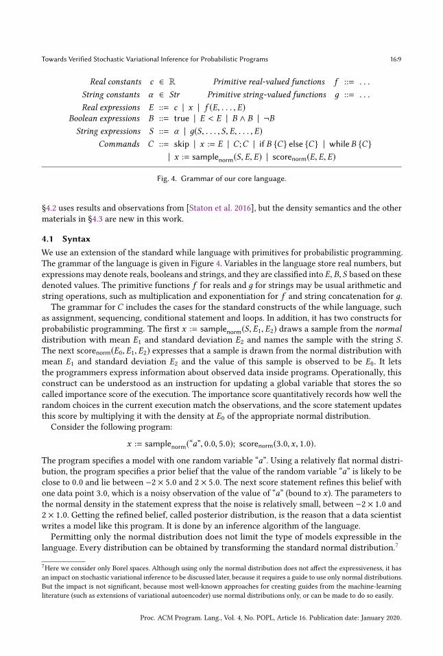
Real constants c ∈ R Primitive real-valued functions f ::= . . .
String constants α ∈ Str Primitive string-valued functions д ::= . . .
Real expressions E ::= c | x | f (E, . . . , E)Boolean expressions B ::= true | E < E | B ∧ B | ¬B
String expressions S ::= α | д(S, . . . , S, E, . . . , E)
Commands C ::= skip | x := E | C;C | if B {C} else {C} | whileB {C}| x := samplenorm(S, E, E) | scorenorm(E, E, E)
Fig. 4. Grammar of our core language.
§4.2 uses results and observations from [Staton et al. 2016], but the density semantics and the other
materials in §4.3 are new in this work.
4.1 SyntaxWe use an extension of the standard while language with primitives for probabilistic programming.
The grammar of the language is given in Figure 4. Variables in the language store real numbers, but
expressions may denote reals, booleans and strings, and they are classified into E,B, S based on thesedenoted values. The primitive functions f for reals and д for strings may be usual arithmetic and
string operations, such as multiplication and exponentiation for f and string concatenation for д.The grammar for C includes the cases for the standard constructs of the while language, such
as assignment, sequencing, conditional statement and loops. In addition, it has two constructs for
probabilistic programming. The first x := samplenorm(S, E1, E2) draws a sample from the normaldistribution with mean E1 and standard deviation E2 and names the sample with the string S .The next scorenorm(E0, E1, E2) expresses that a sample is drawn from the normal distribution with
mean E1 and standard deviation E2 and the value of this sample is observed to be E0. It letsthe programmers express information about observed data inside programs. Operationally, this
construct can be understood as an instruction for updating a global variable that stores the so
called importance score of the execution. The importance score quantitatively records how well the
random choices in the current execution match the observations, and the score statement updates
this score by multiplying it with the density at E0 of the appropriate normal distribution.
Consider the following program:
x := samplenorm(“a”, 0.0, 5.0); scorenorm(3.0, x, 1.0).
The program specifies a model with one random variable “a”. Using a relatively flat normal distri-
bution, the program specifies a prior belief that the value of the random variable “a” is likely to be
close to 0.0 and lie between −2 × 5.0 and 2 × 5.0. The next score statement refines this belief with
one data point 3.0, which is a noisy observation of the value of “a” (bound to x ). The parameters to
the normal density in the statement express that the noise is relatively small, between −2 × 1.0 and2 × 1.0. Getting the refined belief, called posterior distribution, is the reason that a data scientist
writes a model like this program. It is done by an inference algorithm of the language.
Permitting only the normal distribution does not limit the type of models expressible in the
language. Every distribution can be obtained by transforming the standard normal distribution.7
7Here we consider only Borel spaces. Although using only the normal distribution does not affect the expressiveness, it has
an impact on stochastic variational inference to be discussed later, because it requires a guide to use only normal distributions.
But the impact is not significant, because most well-known approaches for creating guides from the machine-learning
literature (such as extensions of variational autoencoder) use normal distributions only, or can be made to do so easily.
Proc. ACM Program. Lang., Vol. 4, No. POPL, Article 16. Publication date: January 2020.

16:10 Wonyeol Lee, Hangyeol Yu, Xavier Rival, and Hongseok Yang
4.2 Measure SemanticsThe denotational semantics of the language just presented is mostly standard, but employs some
twists to address the features for probabilistic programming [Staton et al. 2016].
Here is a short high-level overview of the measure semantics. Our semantics defines multiple
measurable spaces, such as Store and State, that hold mathematical counterparts to the usual actors
in computation, such as program stores (i.e., mappings from variables to values) and states (which
consist of a store and further components). Then, the semantics interprets expressions E,B, S and
commands C as measurable functions of the following types:
⟦E⟧ : Store→ R, ⟦B⟧ : Store→ B, ⟦S⟧ : Store→ Str, ⟦C⟧ : State→ Sp(State × [0,∞)).
Here R is the measurable space of reals with the Borel σ -algebra, and B and Str are discrete
measurable spaces of booleans and strings. Store and State aremeasurable spaces for stores (i.e., maps
from variables to values) and states which consist of a store and a part for recording information
about sampled random variables. Note that the target measurable space of commands is built
by first taking the product of measurable spaces State and [0,∞) and then forming a space out
of subprobability measures on State × [0,∞). This construction indicates that commands denote
probabilistic computations, and the result of each such computation consists of an output state
and a score which expresses how well the computation matches observations expressed with the
score statements in the commandC . Some of the possible outcomes of the computation may lead to
non-termination or an error, and these abnormal outcomes are not accounted for by the semantics,
which is why ⟦C⟧(σ ) for a state σ ∈ Σ is a subprobability distribution. The semantics of expressions
is much simpler. It just says that expressions do not involve any probabilistic computations, so that
they denote deterministic measurable functions.
We now explain how this high-level idea gets implemented in our semantics. Let Var be a
countably infinite set of variables. Our semantics uses the following sets:
Stores s ∈ Store ≜ [Var → R](which is isomorphic to
∏x ∈Var
R)
Random databases r ∈ RDB ≜⋃
K ⊆finStr
[K → R](which is isomorphic to
⋃K ⊆finStr
∏α ∈K
R)
States σ ∈ State ≜ Store × RDB,
where [X → Y ] denotes the set of all functions from X to Y . A state σ consists of a store s and a
random database r . The former fixes the values of variables, and the latter records the name (given
as a string) and the value of each sampled random variable. The domain of r is the names of all
the sampled random variables. By insisting that r should be a map, the semantics asserts that no
two random variables have the same name. For each state σ , we write σs and σr for its store andrandom database components, respectively. Also, for a variable x , a string α and a value v , we writeσ [x 7→ v] and σ [α 7→ v] to mean (σs [x 7→ v],σr ) and (σs ,σr [α 7→ v]).
We equip all of these sets with σ -algebras and turn them to measurable spaces in a standard way.
Note that we constructed the sets from R by repeatedly applying the product and disjoint-union
operators. We equip R with the usual Borel σ -algebra. Then, we parallel each usage of the product
and the disjoint-union operators on sets with that of the corresponding operators on σ -algebras.This gives the σ -algebras for all the sets defined above. Although absent from the above definition,
the measurable spaces B and Str equipped with discrete σ -algebras are also used in our semantics.
We interpret expressions E,B, S as measurable functions ⟦E⟧ : Store → R, ⟦B⟧ : Store → B,and ⟦S⟧ : Store → Str , under the assumption that the semantics of primitive real-valued f of
Proc. ACM Program. Lang., Vol. 4, No. POPL, Article 16. Publication date: January 2020.
Towards Verified Stochastic Variational Inference for Probabilistic Programs 16:11
⟦skip⟧(σ )(A) ≜ 1[(σ ,1)∈A] ⟦x := E⟧(σ )(A) ≜ 1[(σ [x 7→⟦E⟧σs ],1)∈A]⟦C0;C1⟧(σ )(A) ≜
∫ ⟦C0⟧(σ )(d(σ ′,w ′))∫ ⟦C1⟧(σ ′)(d(σ ′′,w ′′))1[(σ ′′,w ′ ·w ′′)∈A]
⟦if B {C0} else {C1}⟧(σ )(A) ≜ 1[⟦B⟧σs=true] · ⟦C0⟧(σ )(A) + 1[⟦B⟧σs,true] · ⟦C1⟧(σ )(A)⟦whileB {C}⟧(σ )(A) ≜ (fix F )(σ )(A)(
where F (κ)(σ )(A) ≜ 1[⟦B⟧σs,true] · 1[(σ ,1)∈A]+ 1[⟦B⟧σs=true] ·
∫ ⟦C⟧(σ )(d(σ ′,w ′)) ∫ κ(σ ′)(d(σ ′′,w ′′))1[(σ ′′,w ′ ·w ′′)∈A])
⟦x := samplenorm(S, E1, E2)⟧(σ )(A) ≜ 1[⟦S⟧σs<dom(σr )] · 1[⟦E2⟧σs ∈(0,∞)]·∫dv
(N(v ; ⟦E1⟧σs , ⟦E2⟧σs ) · 1[((σs [x 7→v],σr [⟦S⟧σs 7→v]),1)∈A]
)⟦scorenorm(E0, E1, E2)⟧(σ )(A) ≜ 1[⟦E2⟧σs ∈(0,∞)] · 1[(σ ,N(⟦E0⟧σs ;⟦E1⟧σs ,⟦E2⟧σs ))∈A]
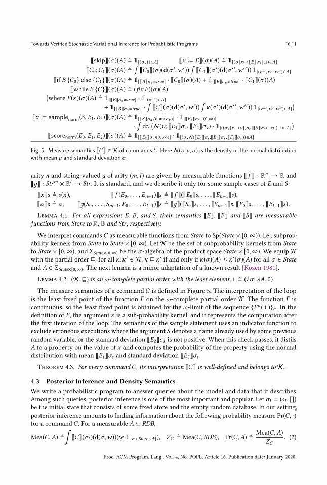
Fig. 5. Measure semantics ⟦C⟧ ∈ K of commandsC . HereN(v ; µ,σ ) is the density of the normal distributionwith mean µ and standard deviation σ .
arity n and string-valued д of arity (m, l) are given by measurable functions ⟦f ⟧ : Rn → R and
⟦д⟧ : Strm × Rl → Str . It is standard, and we describe it only for some sample cases of E and S :
⟦x⟧s ≜ s(x), ⟦f (E0, . . . , En−1)⟧s ≜ ⟦f ⟧(⟦E0⟧s, . . . , ⟦En−1⟧s),⟦α⟧s ≜ α, ⟦д(S0, . . . , Sm−1, E0, . . . , El−1)⟧s ≜ ⟦д⟧(⟦S0⟧s, . . . , ⟦Sm−1⟧s, ⟦E0⟧s, . . . , ⟦El−1⟧s).Lemma 4.1. For all expressions E, B, and S , their semantics ⟦E⟧, ⟦B⟧ and ⟦S⟧ are measurable
functions from Store to R, B and Str , respectively.
We interpret commands C as measurable functions from State to Sp(State × [0,∞)), i.e., subprob-ability kernels from State to State × [0,∞). Let K be the set of subprobability kernels from Stateto State × [0,∞), and ΣState×[0,∞) be the σ -algebra of the product space State × [0,∞). We equip K
with the partial order ⊑: for all κ,κ ′ ∈ K , κ ⊑ κ ′ if and only if κ(σ )(A) ≤ κ ′(σ )(A) for all σ ∈ Stateand A ∈ ΣState×[0,∞). The next lemma is a minor adaptation of a known result [Kozen 1981].
Lemma 4.2. (K, ⊑) is an ω-complete partial order with the least element ⊥ ≜ (λσ . λA. 0).
The measure semantics of a command C is defined in Figure 5. The interpretation of the loop
is the least fixed point of the function F on the ω-complete partial order K . The function F is
continuous, so the least fixed point is obtained by the ω-limit of the sequence {Fn(⊥)}n . In the
definition of F , the argument κ is a sub-probability kernel, and it represents the computation after
the first iteration of the loop. The semantics of the sample statement uses an indicator function to
exclude erroneous executions where the argument S denotes a name already used by some previous
random variable, or the standard deviation ⟦E2⟧σs is not positive. When this check passes, it distils
A to a property on the value of x and computes the probability of the property using the normal
distribution with mean ⟦E1⟧σs and standard deviation ⟦E2⟧σs .Theorem 4.3. For every command C , its interpretation ⟦C⟧ is well-defined and belongs to K .
4.3 Posterior Inference and Density SemanticsWe write a probabilistic program to answer queries about the model and data that it describes.
Among such queries, posterior inference is one of the most important and popular. Let σI = (sI , [])be the initial state that consists of some fixed store and the empty random database. In our setting,
posterior inference amounts to finding information about the following probability measure Pr(C, ·)for a command C . For a measurable A ⊆ RDB,
Mea(C,A) ≜
∫⟦C⟧(σI )(d(σ ,w))(w ·1[σ ∈Store×A]), ZC ≜ Mea(C, RDB), Pr(C,A) ≜
Mea(C,A)
ZC. (2)
Proc. ACM Program. Lang., Vol. 4, No. POPL, Article 16. Publication date: January 2020.
16:12 Wonyeol Lee, Hangyeol Yu, Xavier Rival, and Hongseok Yang
The probability measure Pr(C, ·) is called the posterior distribution of C , and Mea(C, ·) the unnor-malised posterior distribution of C (in Mea(C, ·) and Pr(C, ·), we elide the dependency on sI to avoid
clutter). Finding information about the former is the goal of most inference engines of existing
probabilistic programming languages. Of course, Pr(C, ·) is not defined when the normalising con-
stant ZC is infinite or zero. The inference engines regard such a case as an error that a programmer
should avoid, and consider only C without those errors.
Most algorithms for posterior inference use the density semantics of commands. They implicitly
pick measures on some measurable spaces used in the semantics. These measures are called
reference measures, and constructed out of Lebesgue and counting measures [Bhat et al. 2012,
2013; Hur et al. 2015]. Then, the algorithms interpret commands as density functions with respect
to these measures. One outcome of this density semantics is that the unnormalised posterior
distribution Mea(C, ·) of a command C has a measurable function f : RDB → [0,∞) such that
Mea(C,A) =∫ρ(dr ) (1[r ∈A] · f (r )), where ρ is a reference measure on RDB. Function f is called
density ofMea(C, ·) with respect to ρ.In the rest of this subsection, we define the meanings of commands using density functions. To
do this, we need to set up some preliminary definitions.
First, we look at a predicate and an operator for random databases, which are about the possibility
and the very act of merging two databases. For r , r ′ ∈ RDB, define the predicate r#r ′ by:
r#r ′ ⇐⇒ dom(r ) ∩ dom(r ′) = ∅.
When r#r ′, let r ⊎ r ′ be the random database obtained by merging r and r ′:
dom(r ⊎ r ′) ≜ dom(r ) ∪ dom(r ′); (r ⊎ r ′)(α) ≜ if α ∈ dom(r ) then r (α) else r ′(α).
Lemma 4.4. For every measurable h : RDB × RDB × RDB → R, the function (r , r ′) 7−→ 1[r#r ′] ×
h(r , r ′, r ⊎ r ′) from RDB × RDB to R is measurable.
Second, we define a reference measure ρ on RDB:
ρ(R) ≜∑
K ⊆finStr
(⊗α ∈K
λ)(R ∩ [K → R]),
where λ is the Lebesgue measure on R. As explained in the preliminary section, the symbol ⊗
here represents the operator for constructing a product measure. In particular,
⊗α ∈K λ refers to
the product of the |K | copies of the Lebesgue measure λ on R. In the above definition, we view
functions in [K → R] as tuples with |K | real components and measure sets of such functions using
the product measure
⊗α ∈K λ. When K is the empty set,
⊗α ∈K λ is the nullary-product measure
on {[]}, which assigns 1 to {[]} and 0 to the empty set.
The measure ρ computes the size of each measurable subset R ⊆ RDB in three steps. It splits
a given R into groups based on the domains of elements in R. Then, it computes the size of each
group separately, using the product of the Lebesgue measure. Finally, it adds the computed sizes.
The measure ρ is not finite, but it satisfies the σ -finiteness condition,8 the next best property.Third, we define a partially-ordered set D with certain measurable functions. We say that a
function д : Store × RDB→ {⊥} ∪ (Store × RDB × [0,∞) × [0,∞)) uses random databases locally or
is local if for all s, s ′ ∈ Store, r , r ′ ∈ RDB, andw ′,p ′ ∈ [0,∞),
д(s, r ) = (s ′, r ′,w ′,p ′) =⇒ (∃r ′′. r ′#r ′′ ∧ r = r ′ ⊎ r ′′ ∧ д(s, r ′′) = (s ′, [],w ′,p ′))∧ (∀r ′′′. r#r ′′′ =⇒ д(s, r ⊎ r ′′′) = (s ′, r ′ ⊎ r ′′′,w ′,p ′)).
8The condition lets us use Fubini theorem when showing the well-formedness of the density semantics in this subsection
and relating this semantics with the measure semantics in the previous subsection.
Proc. ACM Program. Lang., Vol. 4, No. POPL, Article 16. Publication date: January 2020.
Towards Verified Stochastic Variational Inference for Probabilistic Programs 16:13
⟦skip⟧d (s, r ) ≜ (s, r , 1, 1) ⟦x :=E⟧d (s, r ) ≜ (s[x 7→ ⟦E⟧s], r , 1, 1)⟦C0;C1⟧d (s, r ) ≜ (⟦C1⟧‡d ◦ ⟦C0⟧d )(s, r )
⟦if B {C0} else {C1}⟧d (s, r ) ≜ if (⟦B⟧s = true) then ⟦C0⟧d (s, r ) else ⟦C1⟧d (s, r )⟦whileB {C}⟧d (s, r ) ≜ (fixG)(s, r )
(where G(д)(s, r ) = if (⟦B⟧s , true) then (s, r , 1, 1) else (д‡ ◦ ⟦C⟧d )(s, r ))⟦x :=samplenorm(S, E1, E2)⟧d (s, r ) ≜ if (⟦S⟧s < dom(r ) ∨ ⟦E2⟧s < (0,∞)) then ⊥
else (s[x 7→ r (⟦S⟧s)], r \ ⟦S⟧s, 1, N(r (⟦S⟧s); ⟦E1⟧s, ⟦E2⟧s))⟦scorenorm(E0, E1, E2)⟧d (s, r ) ≜ if (⟦E2⟧s < (0,∞)) then ⊥ else (s, r ,N(⟦E0⟧s; ⟦E1⟧s, ⟦E2⟧s), 1)
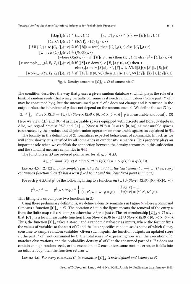
Fig. 6. Density semantics ⟦C⟧d ∈ D of commands C
The condition describes the way that д uses a given random database r , which plays the role of a
bank of random seeds (that д may partially consume as it needs random values). Some part r ′′ of rmay be consumed by д, but the unconsumed part r ′ of r does not change and is returned in the
output. Also, the behaviour of д does not depend on the unconsumed r ′. We define the set D by
D ≜{д : Store × RDB→ {⊥} ∪ (Store × RDB × [0,∞) × [0,∞))
�� д is measurable and local
}. (3)
Here we view {⊥} and [0,∞) as measurable spaces equipped with discrete and Borel σ -algebras.Also, we regard Store × RDB and {⊥} ∪ (Store × RDB × [0,∞) × [0,∞)) as measurable spaces
constructed by the product and disjoint-union operators on measurable spaces, as explained in §3.
The locality in the definition of D formalises expected behaviours of commands. In fact, as we
will show shortly, it is satisfied by all commands in our density semantics. This property plays an
important role when we establish the connection between the density semantics in this subsection
and the standard measure semantics in §4.2.
The functions in D are ordered pointwise: for all д,д′ ∈ D,
д ⊑ д′ ⇐⇒ ∀(s, r ) ∈ Store × RDB. (д(s, r ) = ⊥ ∨ д(s, r ) = д′(s, r )).
Lemma 4.5. (D, ⊑) is an ω-complete partial order and has the least element a 7−→ ⊥. Thus, everycontinuous function G on D has a least fixed point (and this least fixed point is unique).
For eachд ∈ D, letд‡ be the following lifting to a function on {⊥}∪(Store×RDB×[0,∞)×[0,∞)):
д‡(⊥) ≜ ⊥, д‡(s, r ,w,p) ≜
{⊥ if д(s, r ) = ⊥,(s ′, r ′,w ×w ′,p × p ′) if д(s, r ) = (s ′, r ′,w ′,p ′).
This lifting lets us compose two functions in D.
Using these preliminary definitions, we define a density semantics in Figure 6, where a command
C means a function ⟦C⟧d ∈ D. The notation r \v in the figure means the removal of the entry vfrom the finite map r if v ∈ dom(r ); otherwise, r \v is just r . The set membership ⟦C⟧d ∈ D says
that ⟦C⟧d is a local measurable function from Store × RDB to {⊥} ∪ Store × RDB × [0,∞) × [0,∞).Thus, the function ⟦C⟧d takes a store s and a random database r as inputs, where the former fixes
the values of variables at the start of C and the latter specifies random seeds some of which C may
consume to sample random variables. Given such inputs, the function outputs an updated store
s ′, the part r ′ of r not consumed by C , the total scorew ′ expressing how well the execution of Cmatches observations, and the probability density p ′ of C at the consumed part of r . If r does notcontain enough random seeds, or the execution of C encounters some runtime error, or it falls into
an infinite loop, then the function returns ⊥.
Lemma 4.6. For every command C , its semantics ⟦C⟧d is well-defined and belongs to D.
Proc. ACM Program. Lang., Vol. 4, No. POPL, Article 16. Publication date: January 2020.
16:14 Wonyeol Lee, Hangyeol Yu, Xavier Rival, and Hongseok Yang
The density semantics ⟦C⟧d is closely related to the measure semantics ⟦C⟧ defined in §4.2. Both
interpretations ofC describe the computation ofC but from slightly different perspectives. To state
this relationship formally, we need a few notations. For д ∈ D and s ∈ Store, define
dens(д, s) : RDB→ [0,∞), dens(д, s)(r ) ≜{w ′ × p ′ if ∃s ′,w ′,p ′. (д(s, r ) = (s ′, [],w ′,p ′)),0 otherwise,
get(д, s) : RDB→ Store ∪ {⊥}, get(д, s)(r ) ≜{s ′ if ∃s ′,w ′,p ′. (д(s, r ) = (s ′, [],w ′,p ′)),⊥ otherwise.
Both dens(д, s) and get(д, s) are concerned with random databases r that precisely describe the
randomness needed by the execution of д from s . This is formalised by the use of [] in the definitions.
The function dens(д, s) assigns a score to such an r , and in so doing, it defines a probability density
on RDB with respect to the reference measure ρ. The function get(д, s) computes a store that the
computation ofдwould result in when started with such an r . We often write dens(C, s) and get(C, s)to mean dens(⟦C⟧d , s) and get(⟦C⟧d , s), respectively.Lemma 4.7. For all д ∈ D, the following functions from Store × RDB to R and {⊥} ∪ Store are
measurable: (s, r ) 7−→ dens(д, s)(r ) and (s, r ) 7−→ get(д, s)(r ).
The next lemma is the main reason that we considered the locality property. It plays a crucial
role in proving Theorem 4.9, the key result of this subsection.
Lemma 4.8. For all non-negative bounded measurable functions h : ({⊥} ∪ Store) × RDB → R,stores s , and functions д1,д2 ∈ D, we have that∫
ρ(dr )(dens(д‡
2◦ д1, s)(r ) · h
(get(д‡
2◦ д1, s)(r ), r
))=
∫ρ(dr1)
(dens(д1, s)(r1) · 1[get(д1,s)(r1),⊥]
·
∫ρ(dr2)
(dens(д2, get(д1, s)(r1))(r2) · 1[r1#r2] · h
(get(д2, get(д1, s)(r1))(r2), r1 ⊎ r2
))).
Assume that ({⊥}∪ Store)×RDB is ordered as follows: for all (a, r ), (a′, r ′) ∈ ({⊥}∪ Store)×RDB,
(a, r ) ⊑ (a′, r ′) ⇐⇒ (a = ⊥ ∨ a = a′) ∧ r = r ′.
Theorem 4.9. For all non-negative bounded measurable monotone functions h : ({⊥} ∪ Store) ×RDB→ R and states σ ,∫
⟦C⟧(σ )(d(σ ′,w ′)) (w ′ ·h(σ ′s ,σ ′r )) =∫
ρ(dr ′)(dens(C,σs )(r ′) ·1[r ′#σr ] ·h(get(C,σs )(r
′), r ′⊎σr )).
Corollary 4.10. Mea(C,A) =∫ρ(dr ) (1[r ∈A] · dens(C, sI )(r )) for all C and all measurable A.
This corollary says that dens(C, sI ) is the density of the measureMea(C, ·) with respect to ρ, andsupports our informal claim that ⟦C⟧d computes the density of the measure ⟦C⟧.5 STOCHASTIC VARIATIONAL INFERENCEIn this section, we explain stochastic variational inference (SVI) algorithms using the semantics
that we have developed so far. In particular, we describe the requirements made implicitly by one
fundamental SVI algorithm, which is regarded most permissive by the ML researchers because the
algorithm does not require the differentiability of the density of a given probabilistic model.
We call a command C model if it has a finite nonzero normalising constant:
ZC = Mea(C, RDB) =( ∫
⟦C⟧(σI )(d(σ ,w))w)∈ (0,∞),
Proc. ACM Program. Lang., Vol. 4, No. POPL, Article 16. Publication date: January 2020.

Towards Verified Stochastic Variational Inference for Probabilistic Programs 16:15
model C ≡(s := samplenorm(“slope”, 0.0, 5.0); i := samplenorm(“intercept”, 0.0, 5.0);x1 := 1.0; y1 := 2.3; x2 := 2.0; y2 := 4.2; x3 := 3.0; y3 := 6.9;scorenorm(y1, s · x1 + i, 1.0); scorenorm(y2, s · x2 + i, 1.0); scorenorm(y3, s · x3 + i, 1.0)
)guide Dθ ≡
(s := samplenorm(“slope”, θ1, exp(θ2)); i := samplenorm(“intercept”, θ3, exp(θ4))
)Fig. 7. Example model-guide pair for simple Bayesian linear regression.
where σI is the initial state. Given a model C , the SVI algorithms attempt to infer a good approx-
imation of C’s posterior distribution Pr(C, ·) defined in (2). They tackle this posterior-inference
problem in two steps.
First, the SVI algorithms fix a collection of approximate distributions. They usually do so by
asking the developer ofC to provide a command Dθ parameterised by θ ∈ Rp , which can serve as a
template for approximation distributions. The command Dθ typically has a control-flow structure
similar to that of C , but it is simpler than C: it does not use any score statements, and may replace
complex computation steps ofC by simpler ones. In fact,Dθ should satisfy two formal requirements,
which enforce this simplicity. The first is
Mea(Dθ , RDB) = 1 for all θ ∈ Rp,
which means that the normalising constant of Dθ is 1. The second is that Dθ should keep the score
(i.e., thew component) to be 1, i.e.,
⟦Dθ ⟧(σI )(State × ([0,∞) \ {1})) = 0.
Meeting these requirements is often not too difficult. A common technique is to ensure that Dθ does
not use the score statement and always terminates. Figure 7 gives an example of (C,Dθ ) for simple
Bayesian linear regression with three data points. Note that in this case, Dθ is obtained from C by
deleting the score statements and replacing the arguments 0.0 and 5.0 of normal distributions by
parameter θ = (θ1, θ2, θ3, θ4). Following the terminology of Pyro, we call a parameterised command
Dθ guide if it satisfies the two requirements just mentioned.
Second, the SVI algorithms search for a good parameter θ that makes the distribution described
by Dθ close to the posterior of C . Concretely, they formulate an optimisation problem where the
optimisation objective expresses that some form of distance from Dθ ’s distribution to C’s posteriorshould be minimised. Then, they solve the problem by a version of gradient descent.
The KL divergence is a standard choice for distance. Let µ, µ ′ be measures on RDB that have
densities д and д′ with respect to the measure ρ. The KL divergence from д to д′ is defined by
KL(д | |д′) ≜
∫ρ(dr )
(д(r ) · log
д(r )
д′(r )
). (4)
In words, it is the ratio of densities д and д′ averaged according to д. If д = д′, the ratio is always 1,
so that the KL becomes 0. The KL divergence is defined only if the following conditions are met:
• Absolute continuity: д′(r ) = 0 =⇒ д(r ) = 0 for all r ∈ RDB,9 which ensures that the
integrand in (4) is well-defined even when the denominator д′(r ) in (4) takes the value 0;
• Integrability: the integral in (4) has a finite value.
Using our semantics, we can express the KL objective as follows:
argminθ ∈RpKL
(dens(Dθ , sI )
������dens(C, sI )ZC
). (5)
9This condition can be relaxed in a more general formulation of the KL divergence stated in terms of the so called Radon-
Nikodym derivative. We do not use the relaxed condition to reduce the amount of materials on measure theory in the paper.
Proc. ACM Program. Lang., Vol. 4, No. POPL, Article 16. Publication date: January 2020.
16:16 Wonyeol Lee, Hangyeol Yu, Xavier Rival, and Hongseok Yang
Recall that dens(Dθ , sI ) and dens(C, sI )/ZC are densities of the probability measures of the command
Dθ and the posterior of C (Corollary 4.10), and they are defined by means of our density semantics
in §4.3. Most SVI engines solve this optimisation problem by a version of gradient descent.
In the paper, we consider one of themost fundamental and versatile SVI algorithms. The algorithm
is called score estimator or REINFORCE, and it works by estimating the gradient of the objective in
(5) using samples and performing the gradient descent with this estimated gradient. More concretely,
the algorithm starts by initialising θ with some value (usually chosen randomly) and updating it
repeatedly by the following procedure:
(i) Sample r1, . . . , rN independently from dens(Dθ , sI )
(ii) θ ← θ − η ×
(1
N
N∑i=1
(∇θ log dens(Dθ , sI )(ri )
)· log
dens(Dθ , sI )(ri )
dens(C, sI )(ri )
)Here N and η are hyperparameters to this algorithm, the former determining the number of samples
used to estimate the gradient and the latter, called learning rate, deciding how much the algorithm
should follow the direction of the estimated gradient. Although we do not explain here, sampling
r1, . . . , rN and computing all of dens(Dθ , sI )(ri ), dens(C, sI )(ri ) and ∇θ (log dens(Dθ , sI )(ri )) can be
done by executing Dθ and C multiple times under slightly unusual operational semantics [Yang
2019]. The SVI engines of Pyro and Anglican implement such operational semantics.
The average over the N terms in the θ -update step is the core of the algorithm. It approximates
the gradient of the optimisation objective in (5):
∇θKL
(dens(Dθ , sI )
������dens(C, sI )ZC
)≈
1
N
N∑i=1
(∇θ log dens(Dθ , sI )(ri )
)· log
dens(Dθ , sI )(ri )
dens(C, sI )(ri ).
The average satisfies an important property called unbiasedness, summarised by Theorem 5.1.
Theorem 5.1. Let C be a model, Dθ be a guide, and N , 0 ∈ N. Define KL(−) : Rp → R≥0 as KLθ≜ KL(dens(Dθ , sI )| |dens(C, sI )/ZC ). Then, KL(−) is well-defined and continuously differentiable with
∇θKLθ = E∏i dens(Dθ ,sI )(ri )
[1
N
N∑i=1
(∇θ log dens(Dθ , sI )(ri )
)log
dens(Dθ , sI )(ri )
dens(C, sI )(ri )
](6)
if(R1) dens(C, sI )(r ) = 0 =⇒ dens(Dθ , sI )(r ) = 0, for all r ∈ RDB and θ ∈ Rp ;(R2) for all (r , θ, j) ∈ RDB × Rp × [p], the function v 7−→ dens(Dθ [j :v], sI )(r ) on R is differentiable;(R3) for all θ ∈ Rp , ∫
ρ(dr )
(dens(Dθ , sI )(r ) · log
dens(Dθ , sI )(r )
dens(C, sI )(r )
)< ∞;
(R4) for all (θ , j) ∈ Rp × [p], the function
v 7−→
∫ρ(dr )
(dens(Dθ [j :v], sI )(r ) · log
dens(Dθ [j :v], sI )(r )
dens(C, sI )(r )
)on R is continuously differentiable;
(R5) for all θ ∈ Rp ,
∇θ
∫ρ(dr )
(dens(Dθ , sI )(r ) · log
dens(Dθ , sI )(r )
dens(C, sI )(r )
)=
∫ρ(dr ) ∇θ
(dens(Dθ , sI )(r ) · log
dens(Dθ , sI )(r )
dens(C, sI )(r )
);
(R6) for all θ ∈ Rp , ∫ρ(dr ) ∇θ dens(Dθ , sI )(r ) = ∇θ
∫ρ(dr ) dens(Dθ , sI )(r ).
Here θ [j : v] denotes a vector in Rp that is the same as θ except that its j-th component is v .
Proc. ACM Program. Lang., Vol. 4, No. POPL, Article 16. Publication date: January 2020.
Towards Verified Stochastic Variational Inference for Probabilistic Programs 16:17
The conclusion of this theorem (Equation (6)) and its proof are well-known [Ranganath et al. 2014],
but the requirements in the theorem (and the continuous differentiability of KLθ in the conclusion)
are rarely stated explicitly in the literature.
The correctness of the algorithm crucially relies on the unbiasedness property in Theorem 5.1.
The property ensures that the algorithm converges to a local minimum with probability 1. Thus, it
is important that the requirements in the theorem are met. In fact, some of the requirements there
are needed even to state the optimisation objective in (5), because without them, the objective does
not exist. In the next section, we describe conditions that imply those requirements and can serve
as target properties of program analysis for probabilistic programs. The latter point is worked out
in detail in §7 and §8 where we discuss program analysis for probabilistic programs and SVI.
6 CONDITIONS FOR STOCHASTIC VARIATIONAL INFERENCEIdeally wewant to have program analysers that discharge the six requirements R1-R6 in Theorem 5.1.
However, except R1 and R2, the requirements are not ready for serving as the targets of static
analysis algorithms. Automatically discharging them based on the first principles (such as the
definition of integrability with respect to a measure) may be possible, but seems less immediate
than doing so using powerful theorems from continuous mathematics.
In this section, we explain conditions that imply the requirements R3-R6 and are more friendly
to program analysis than the requirements themselves. The conditions are given in two boxes (9)
and (10). Throughout the section, we fix a model C and a guide Dθ .
6.1 AssumptionThroughout the section, we assume that the densities of Dθ and C have the following form:
dens(Dθ , sI )(r ) =M∑i=1
1[r ∈Ai ]
∏α ∈Ki
N(r (α); µ(i ,α )(θ ),σ(i ,α )(θ )
), (7)
dens(C, sI )(r ) =M∑i=1
1[r ∈Ai ]
( ∏α ∈Ki
N(r (α); µ ′
(i ,α )(r ),σ′(i ,α )(r )
)) ©«∏j ∈[Ni ]
N(c(i , j); µ
′′(i , j)(r ),σ
′′(i , j)(r )
)ª®¬ ,where
• M,Ni ∈ N \ {0};• A1, . . . ,AM are disjoint measurable subsets of RDB;• Ki ’s are finite sets of strings such that dom(r ) = Ki for all r ∈ Ai ;
• µ(i ,α ) and σ(i ,α ) are measurable functions from Rp to R and (0,∞), respectively;• µ ′(i ,α ) and µ ′′
(i , j) are measurable functions from [Ki → R] to R;
• σ ′(i ,α ) and σ
′′(i , j) are measurable functions from [Ki → R] to (0,∞);
• c(i , j) is a real number.
In programming terms, our assumption first implies that bothC and Dθ use at most a fixed number
of random variables. That is, the number of random variables they generate must be finite not only
within a single execution but also across all possible executions since the names of all random
variables are found in a finite set
⋃Mi=1 Ki . This property is met if the number of steps in every
execution of C and Dθ from σI is bounded by some T and the executions over the same program
path use the same set of random variables. Note that the bound may depend on sI . Such a bound
exists for most probabilistic programs.10Also, the assumption says that the parameters of normal
distributions in sample statements in Dθ may depend only on θ , but not on other sampled random
10Notable exceptions are models using probabilistic grammars or those from Bayesian nonparametrics.
Proc. ACM Program. Lang., Vol. 4, No. POPL, Article 16. Publication date: January 2020.

16:18 Wonyeol Lee, Hangyeol Yu, Xavier Rival, and Hongseok Yang
variables. This is closely related to a common approach for designing approximate distributions in
variational inference, called mean-field approximation, where the approximate distribution consists
of independent normal random variables.
We use the term “assumption” here, instead of “condition” in the following subsections because
the assumed properties are rather conventional and they are not directly related to the requirements
in Theorem 5.1, at least not as much as the conditions that we will describe next.
6.2 Condition for Requirement R3Note that the integral in the requirement R3 can be written as the sum of two expectations:∫
ρ(dr )
(dens(Dθ , sI )(r ) · log
dens(Dθ , sI )(r )
dens(C, sI )(r )
)= Edens(Dθ ,sI )(r ) [log dens(Dθ , sI )(r )] − Edens(Dθ ,sI )(r ) [log dens(C, sI )(r )] . (8)
The minus of the first term (i.e., −Edens(Dθ ,sI )(r ) [log dens(Dθ , sI )(r )]) is called the differentialentropy of the density dens(Dθ , sI ). Intuitively, it is large when the density on Rn is close to the
Lebesgue measure, which is regarded to represent the absence of information. The differential
entropy is sometimes undefined [Ghourchian et al. 2017]. Fortunately, a large class of proba-
bility densities (containing many commonly used probability distributions) have well-defined
entropies [Ghourchian et al. 2017; Nair et al. 2006]. Our dens(Dθ , sI ) is one of such fortunate cases.
Theorem 6.1. Edens(Dθ ,sI )(r ) [| log dens(Dθ , sI )(r )|] < ∞ under our assumption in §6.1.
We remark that a violation of the assumption (7) for Dθ can result in an undefined entropy, as
illustrated by the following examples.
Example 6.2. Consider guides D(i ,θ ) defined as follows (i = 1, 2):
D(i ,θ ) ≡ (x1 := samplenorm(“a1”, θ1, 1); x2 := samplenorm(“a2”, θ2, Ei [x1]))
where for some n ≥ 1 and c , 0 ∈ R,11
E1[x1] ≡ if (x1=0) then 1 else exp(−1/|x1 |n), E2[x1] ≡ exp(exp(c · x31)).
None of dens(D(i ,θ ), sI )’s satisfies the assumption (7) because the standard deviation of the normal
distribution for x2 depends on the value of x1. The entropies of dens(D(i ,θ ), sI )’s are all undefined:Edens(D(i ,θ ),sI )(r )[| log dens(D(i ,θ ), sI )(r )|] = ∞ for all i = 1, 2. □
Since the first term of (8) is always finite by Theorem 6.1, it is enough to ensure the finiteness of
the second term of (8). For i ∈ [M], define the set of (absolute) affine functions on [Ki → R] as:
Ai ≜{f ∈ [[Ki → R] → R]
��� f (r ) = c +∑α ∈Ki
(cα · |r (α)|) for some c, cα ∈ R}.
Our condition for ensuring the finiteness of the second term is as follows:
For all i ∈ [M], there are f ′, f ′′, l ′,u ′, l ′′,u ′′ ∈ Ai such that
|µ ′(i ,α )(r )| ≤ exp(f ′(r )), exp(l ′(r )) ≤ σ ′
(i ,α )(r ) ≤ exp(u ′(r )),
|µ ′′(i , j)(r )| ≤ exp(f ′′(r )), exp(l ′′(r )) ≤ σ ′′
(i , j)(r ) ≤ exp(u ′′(r )),
all four hold for every (α, j, r ) ∈ Ki × [Ni ] ×Ai .
(9)
Theorem 6.3. The condition (9) implies Edens(Dθ ,sI )(r ) [| log dens(C, sI )(r )|] < ∞ under our assump-tion in §6.1. Thus, in that case, it entails the requirement R3 (i.e., the objective in (5) is well-defined).11Formally, we should implement E1[x1] as an application of a primitive function f1 to x1 that has the semantics described
by the if-then-else statement here.
Proc. ACM Program. Lang., Vol. 4, No. POPL, Article 16. Publication date: January 2020.
Towards Verified Stochastic Variational Inference for Probabilistic Programs 16:19
Our condition in (9) is sufficient but not necessary for the objective in (5) to be defined. However,
its violation is a good warning, as illustrated by our next examples.
Example 6.4. Consider models C1, . . . ,C4 and a guide Dθ defined as follows:
Ci ≡ (x1 := samplenorm(“a1”, 0, 1); x2 := samplenorm(“a2”, Ei [x1], 1)) for i = 1, 2
Ci ≡ (x1 := samplenorm(“a1”, 0, 1); x2 := samplenorm(“a2”, 0, Ei [x1])) for i = 3, 4
Dθ ≡ (x1 := samplenorm(“a1”, θ1, 1); x2 := samplenorm(“a2”, θ2, 1))
where for some n ≥ 1 and c , 0 ∈ R,
E1[x1] ≡ if (x1=0) then 0 else1
xn1
, E2[x1] ≡E4[x1] ≡ exp(c ·x31), E3[x1] ≡ if (x1=0) then 1 else |x1 |n .
Let A = [{“a1”, “a2”} → R]. For r ∈ A, define
µ ′1(r ) ≜ if r (“a1”) = 0 then 0 else 1/r (“a1”)
n, µ ′2(r ) ≜ exp(c · r (“a1”)
3),
σ ′3(r ) ≜ if r (“a1”) = 0 then 1 else |r (“a1”)|
n, σ ′4(r ) ≜ exp(c · r (“a1”)
3).
Then, we have that
dens(Ci , sI )(r ) = 1[r ∈A] · N(r (“a1”); 0, 1) · N(r (“a2”); µ′i (r ), 1) for i = 1, 2
dens(Ci , sI )(r ) = 1[r ∈A] · N(r (“a1”); 0, 1) · N(r (“a2”); 0,σ′i (r )) for i = 3, 4
dens(Dθ , sI )(r ) = 1[r ∈A] · N(r (“a1”);θ1, 1) · N(r (“a2”);θ2, 1).
None of µ ′1, µ ′
2, σ ′
3, and σ ′
4satisfies the condition in (9). The function µ ′
1is not bounded in {r ∈
A | −1 ≤ r (“a1”) ≤ 1 ∧ −1 ≤ r (“a2”) ≤ 1}, but every µ ′ satisfying the condition in (9) should be
bounded. Also, the cubic exponential growth of µ ′2cannot be bounded by any linear exponential
function on r . The violation of the condition by σ ′3and σ ′
4can be shown similarly.
In fact, the objective in (5) is not defined for all of the four cases. This is because for all i = 1, . . . , 4,Edens(Dθ ,sI )(r ) [| log dens(Ci , sI )(r )|] = ∞. □
We now show that the condition in (9) is satisfied by a large class of functions in machine
learning applications, including functions using neural networks. We call a function nn : Rn → Ran affine-bounded neural network if there exist functions fj : R
nj → Rnj+1 and affine functions
lj : Rnj → R for all 1 ≤ j ≤ d such that (i) n1 = n and nd+1 = 1; (ii) nn = fd ◦ · · · ◦ f1; and(iii) ∥ fj (v)∥1 ≤ lj (|v1 |, . . . , |vnj |) for all 1 ≤ j ≤ d and v ∈ Rnj , where ∥ · ∥1 denotes the ℓ1-norm.
Note that each component of fj can be, for instance, an affine function, one of commonly used
activation functions (e.g., relu, tanh, sigmoid, softplus), or one of min/max functions (min andmax).
Therefore, most of neural networks used inmachine learning applications are indeed affine-bounded.
Lemma 6.5 indicates that a wide range of functions satisfy the condition (9).
Lemma 6.5. Pick i ∈ [M] and α ∈ Ki . Let (α1, . . . ,α J ) be an enumeration of the elements in Ki , andr ≜ (r (α1), . . . , r (α J )) ∈ R
J be an enumeration of the values of r ∈ Ai . Consider any affine-boundedneural network nn : RJ → R, polynomial poly : RJ → R, and c ∈ (0,∞). Then, the below list offunctions µ ′
(i ,α ) and σ′(i ,α ) on Ai satisfy the condition in (9):
µ ′(i ,α )(r ) = nn(r ), µ ′
(i ,α )(r ) = poly(r ), µ ′(i ,α )(r ) = exp(nn(r )),
σ ′(i ,α )(r ) = |nn(r )| + c, σ ′
(i ,α )(r ) = |poly(r )| + c, σ ′(i ,α )(r ) = exp(nn(r )),
σ ′(i ,α )(r ) = (|nn(r )| + c)
−1, σ ′(i ,α )(r ) = (|poly(r )| + c)
−1, σ ′(i ,α )(r ) = softplus(nn(r )),
where softplus(v) ≜ log(1 + exp(v)). Moreover, the same holds for µ ′′(i , j) and σ
′′(i , j) as well.
Proc. ACM Program. Lang., Vol. 4, No. POPL, Article 16. Publication date: January 2020.
16:20 Wonyeol Lee, Hangyeol Yu, Xavier Rival, and Hongseok Yang
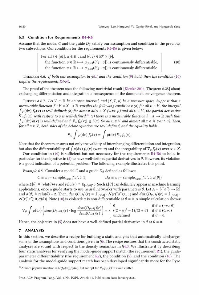
6.3 Condition for Requirements R4-R6Assume that the model C and the guide Dθ satisfy our assumption and condition in the previous
two subsections. Our condition for the requirements R4-R6 is given below:
For all i ∈ [M], α ∈ Ki , and (θ , j) ∈ Rp × [p],
the function v ∈ R 7−→ µ(i ,α )(θ [j : v]) is continuously differentiable;
the function v ∈ R 7−→ σ(i ,α )(θ [j : v]) is continuously differentiable.
(10)
Theorem 6.6. If both our assumption in §6.1 and the condition (9) hold, then the condition (10)
implies the requirements R4-R6.
The proof of the theorem uses the following nontrivial result [Klenke 2014, Theorem 6.28] about
exchanging differentiation and integration, a consequence of the dominated convergence theorem.
Theorem 6.7. Let V ⊂ R be an open interval, and (X , Σ, µ) be a measure space. Suppose that ameasurable function f : V × X → R satisfies the following conditions: (a) for all v ∈ V , the integral∫µ(dx) fv (x) is well-defined; (b) for almost all x ∈ X (w.r.t. µ) and all v ∈ V , the partial derivative∇v fv (x) with respect to v is well-defined;12 (c) there is a measurable function h : X → R such that∫µ(dx)h(x) is well-defined and |∇v fv (x)| ≤ h(x) for all v ∈ V and almost all x ∈ X (w.r.t. µ). Then,
for all v ∈ V , both sides of the below equation are well-defined, and the equality holds:
∇v
∫µ(dx) fv (x) =
∫µ(dx) ∇v fv (x).
Note that the theorem ensures not only the validity of interchanging differentiation and integration,
but also the differentiability of
∫µ(dx) fv (x) (w.r.t. v) and the integrability of ∇v fv (x) over x ∈ X .
Our condition in (10) is sufficient but not necessary for the requirements R4-R6 to hold, in
particular for the objective in (5) to have well-defined partial derivatives in θ . However, its violationis a good indication of a potential problem. The following example illustrates this point.
Example 6.8. Consider a model C and a guide Dθ defined as follows:
C ≡ x := samplenorm(“a”, 0, 1) Dθ ≡ x := samplenorm(“a”, 0, E[θ ])
where E[θ ] ≡ relu(θ )+2 and relu(v) ≜ 1[v≥0] ·v . Such E[θ ] can definitely appear inmachine learning
applications, once a guide starts to use neural networks with parameters θ . Let A = [{“a”} → R]and σ (θ ) ≜ relu(θ ) + 2. Then, dens(C, sI )(r ) = 1[r ∈A] · N(r (“a”); 0, 1) and dens(Dθ , sI )(r ) = 1[r ∈A] ·N(r (“a”); 0,σ (θ )). Note (10) is violated: σ is non-differentiable at θ = 0. A simple calculation shows:
∇θ
∫ρ(dr )
(dens(Dθ , sI )(r ) · log
dens(Dθ , sI )(r )
dens(C, sI )(r )
)=
0 if θ ∈ (−∞, 0)((2 + θ )2 − 1)/(2 + θ ) if θ ∈ (0,∞)undefined if θ = 0.
Hence, the objective in (5) does not have a well-defined partial derivative in θ at θ = 0. □
7 ANALYSISIn this section, we describe a recipe for building a static analysis that automatically discharges
some of the assumptions and conditions given in §6. The recipe ensures that the constructed static
analyses are sound with respect to the density semantics in §4.3. We illustrate it by describing
four static analyses for verifying the model-guide support match (the requirement R1), the guide-
parameter differentiability (the requirement R2), the condition (9), and the condition (10). The
analysis for the model-guide support match has been developed significantly more for the Pyro
12A more popular notation is (∂fv (x ))/(∂v), but we opt for ∇v fv (x ) to avoid clutter.
Proc. ACM Program. Lang., Vol. 4, No. POPL, Article 16. Publication date: January 2020.
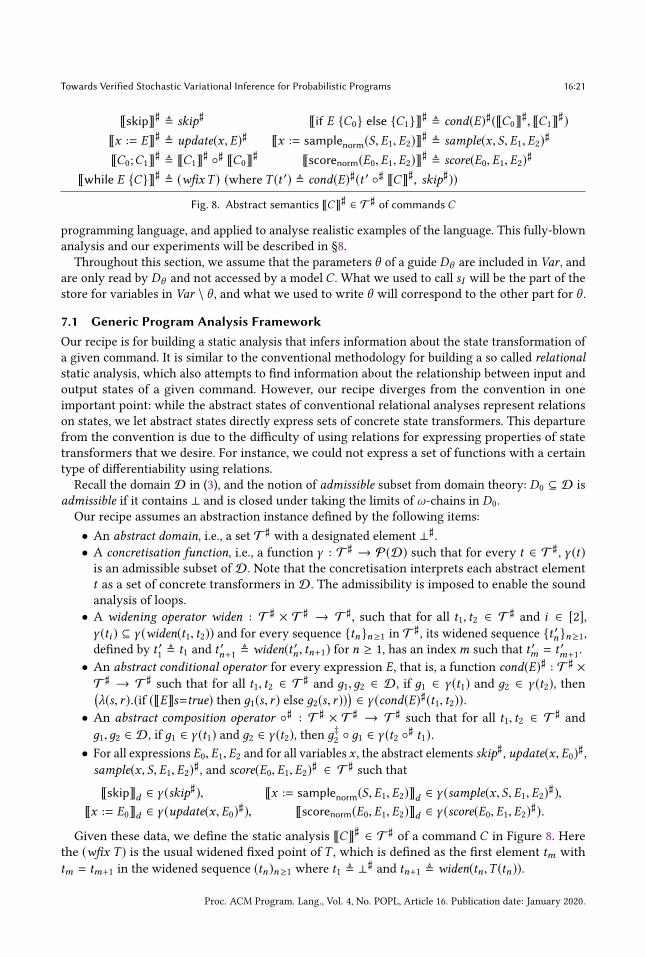
Towards Verified Stochastic Variational Inference for Probabilistic Programs 16:21
⟦skip⟧♯ ≜ skip♯ ⟦if E {C0} else {C1}⟧♯ ≜ cond(E)♯(⟦C0⟧♯, ⟦C1⟧♯)⟦x := E⟧♯ ≜ update(x, E)♯ ⟦x := samplenorm(S, E1, E2)⟧♯ ≜ sample(x, S, E1, E2)♯
⟦C0;C1⟧♯ ≜ ⟦C1⟧♯ ◦♯ ⟦C0⟧♯ ⟦scorenorm(E0, E1, E2)⟧♯ ≜ score(E0, E1, E2)♯
⟦while E {C}⟧♯ ≜ (wfixT ) (where T (t ′) ≜ cond(E)♯(t ′ ◦♯ ⟦C⟧♯, skip♯))Fig. 8. Abstract semantics ⟦C⟧♯ ∈ T ♯ of commands C
programming language, and applied to analyse realistic examples of the language. This fully-blown
analysis and our experiments will be described in §8.
Throughout this section, we assume that the parameters θ of a guide Dθ are included in Var , andare only read by Dθ and not accessed by a model C . What we used to call sI will be the part of thestore for variables in Var \ θ , and what we used to write θ will correspond to the other part for θ .
7.1 Generic Program Analysis FrameworkOur recipe is for building a static analysis that infers information about the state transformation of
a given command. It is similar to the conventional methodology for building a so called relationalstatic analysis, which also attempts to find information about the relationship between input and
output states of a given command. However, our recipe diverges from the convention in one
important point: while the abstract states of conventional relational analyses represent relations
on states, we let abstract states directly express sets of concrete state transformers. This departure
from the convention is due to the difficulty of using relations for expressing properties of state
transformers that we desire. For instance, we could not express a set of functions with a certain
type of differentiability using relations.
Recall the domain D in (3), and the notion of admissible subset from domain theory: D0 ⊆ D is
admissible if it contains ⊥ and is closed under taking the limits of ω-chains in D0.
Our recipe assumes an abstraction instance defined by the following items:
• An abstract domain, i.e., a set T ♯with a designated element ⊥♯
.
• A concretisation function, i.e., a function γ : T ♯ → P(D) such that for every t ∈ T ♯, γ (t)
is an admissible subset of D. Note that the concretisation interprets each abstract element
t as a set of concrete transformers in D. The admissibility is imposed to enable the sound
analysis of loops.
• A widening operator widen : T ♯ × T ♯ → T ♯, such that for all t1, t2 ∈ T♯and i ∈ [2],
γ (ti ) ⊆ γ (widen(t1, t2)) and for every sequence {tn}n≥1 in T♯, its widened sequence {t ′n}n≥1,
defined by t ′1≜ t1 and t
′n+1 ≜ widen(t ′n, tn+1) for n ≥ 1, has an indexm such that t ′m = t ′m+1.
• An abstract conditional operator for every expression E, that is, a function cond(E)♯ : T ♯ ×
T ♯ → T ♯such that for all t1, t2 ∈ T
♯and д1,д2 ∈ D, if д1 ∈ γ (t1) and д2 ∈ γ (t2), then(
λ(s, r ).(if (⟦E⟧s=true) then д1(s, r ) else д2(s, r ))) ∈ γ (cond(E)♯(t1, t2)).• An abstract composition operator ◦♯ : T ♯ × T ♯ → T ♯
such that for all t1, t2 ∈ T♯and
д1,д2 ∈ D, if д1 ∈ γ (t1) and д2 ∈ γ (t2), then д‡2◦ д1 ∈ γ (t2 ◦
♯ t1).
• For all expressions E0, E1, E2 and for all variables x , the abstract elements skip♯ , update(x, E0)♯ ,sample(x, S, E1, E2)♯ , and score(E0, E1, E2)♯ ∈ T ♯
such that
⟦skip⟧d ∈ γ (skip♯), ⟦x := samplenorm(S, E1, E2)⟧d ∈ γ (sample(x, S, E1, E2)♯),⟦x := E0⟧d ∈ γ (update(x, E0)♯), ⟦scorenorm(E0, E1, E2)⟧d ∈ γ (score(E0, E1, E2)♯).
Given these data, we define the static analysis ⟦C⟧♯ ∈ T ♯of a command C in Figure 8. Here
the (wfix T ) is the usual widened fixed point of T , which is defined as the first element tm with
tm = tm+1 in the widened sequence (tn)n≥1 where t1 ≜ ⊥♯and tn+1 ≜ widen(tn,T (tn)).
Proc. ACM Program. Lang., Vol. 4, No. POPL, Article 16. Publication date: January 2020.
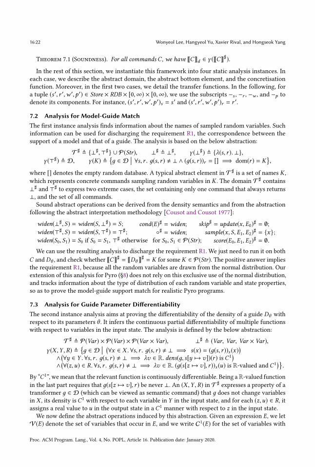
16:22 Wonyeol Lee, Hangyeol Yu, Xavier Rival, and Hongseok Yang
Theorem 7.1 (Soundness). For all commands C , we have ⟦C⟧d ∈ γ (⟦C⟧♯).In the rest of this section, we instantiate this framework into four static analysis instances. In
each case, we describe the abstract domain, the abstract bottom element, and the concretisation
function. Moreover, in the first two cases, we detail the transfer functions. In the following, for
a tuple (s ′, r ′,w ′,p ′) ∈ Store × RDB × [0,∞) × [0,∞), we use the subscripts −s , −r , −w , and −p to
denote its components. For instance, (s ′, r ′,w ′,p ′)s = s′and (s ′, r ′,w ′,p ′)r = r
′.
7.2 Analysis for Model-Guide MatchThe first instance analysis finds information about the names of sampled random variables. Such
information can be used for discharging the requirement R1, the correspondence between the
support of a model and that of a guide. The analysis is based on the below abstraction:
T ♯ ≜ {⊥♯,⊤♯} ∪ P(Str), ⊥♯ ≜ ⊥♯, γ (⊥♯) ≜ {λ(s, r ).⊥},
γ (⊤♯) ≜ D, γ (K) ≜{д ∈ D
�� ∀s, r . д(s, r ) , ⊥ ∧ (д(s, r ))r = [] =⇒ dom(r ) = K},
where [] denotes the empty random database. A typical abstract element in T ♯is a set of names K ,
which represents concrete commands sampling random variables in K . The domain T ♯contains
⊥♯and ⊤♯
to express two extreme cases, the set containing only one command that always returns
⊥, and the set of all commands.
Sound abstract operations can be derived from the density semantics and from the abstraction
following the abstract interpretation methodology [Cousot and Cousot 1977]:
widen(⊥♯, S) = widen(S,⊥♯) = S ;
widen(⊤♯, S) = widen(S,⊤♯) = ⊤♯;
widen(S0, S1) = S0 if S0 = S1, ⊤♯otherwise for S0, S1 ∈ P(Str);
cond(E)♯ = widen;◦♯ = widen;
skip♯ = update(x, E0)♯ = ∅;sample(x, S, E1, E2)♯ = {x};
score(E0, E1, E2)♯ = ∅.
We can use the resulting analysis to discharge the requirement R1. We just need to run it on both
C and Dθ , and check whether ⟦C⟧♯ = ⟦Dθ ⟧♯ = K for some K ∈ P(Str). The positive answer implies
the requirement R1, because all the random variables are drawn from the normal distribution. Our
extension of this analysis for Pyro (§8) does not rely on this exclusive use of the normal distribution,
and tracks information about the type of distribution of each random variable and state properties,
so as to prove the model-guide support match for realistic Pyro programs.
7.3 Analysis for Guide Parameter DifferentiabilityThe second instance analysis aims at proving the differentiability of the density of a guide Dθ with
respect to its parameters θ . It infers the continuous partial differentiability of multiple functions
with respect to variables in the input state. The analysis is defined by the below abstraction:
T ♯ ≜ P(Var) × P(Var) × P(Var × Var), ⊥♯ ≜ (Var, Var, Var × Var),γ (X ,Y ,R) ≜
{д ∈ D
�� (∀x ∈ X .∀s, r . д(s, r ) , ⊥ =⇒ s(x) = (д(s, r ))s (x)
)∧(∀y ∈ Y .∀s, r . д(s, r ) , ⊥ =⇒ λv ∈ R. dens(д, s[y 7→ v])(r ) is C1
)∧(∀(z,u) ∈ R.∀s, r . д(s, r ) , ⊥ =⇒ λv ∈ R. (д(s[z 7→ v], r ))s (u) is R-valued and C1
)}.
By “C1”, wemean that the relevant function is continuously differentiable. Being aR-valued function
in the last part requires that д(s[z 7→ v], r ) be never ⊥. An (X ,Y ,R) in T ♯expresses a property of a
transformer д ∈ D (which can be viewed as semantic command) that д does not change variables
in X , its density isC1with respect to each variable in Y in the input state, and for each (z,u) ∈ R, it
assigns a real value to u in the output state in a C1manner with respect to z in the input state.
We now define the abstract operations induced by this abstraction. Given an expression E, we letV(E) denote the set of variables that occur in E, and we write C1(E) for the set of variables with
Proc. ACM Program. Lang., Vol. 4, No. POPL, Article 16. Publication date: January 2020.
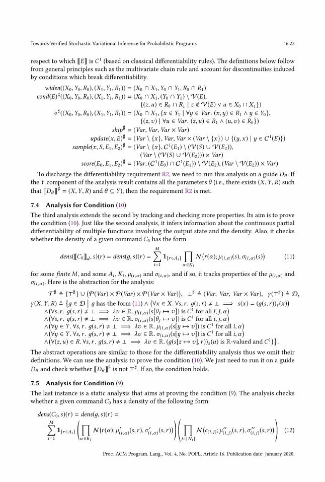
Towards Verified Stochastic Variational Inference for Probabilistic Programs 16:23
respect to which ⟦E⟧ is C1(based on classical differentiability rules). The definitions below follow
from general principles such as the multivariate chain rule and account for discontinuities induced
by conditions which break differentiability.
widen((X0,Y0,R0), (X1,Y1,R1)) = (X0 ∩ X1,Y0 ∩ Y1,R0 ∩ R1)
cond(E)♯((X0,Y0,R0), (X1,Y1,R1)) = (X0 ∩ X1, (Y0 ∩ Y1) \ V(E),{(z,u) ∈ R0 ∩ R1 | z < V(E) ∨ u ∈ X0 ∩ X1})
◦♯((X0,Y0,R0), (X1,Y1,R1)) = (X0 ∩ X1, {x ∈ Y1 | ∀y ∈ Var . (x,y) ∈ R1 ∧ y ∈ Y0},{(z,v) | ∀u ∈ Var . (z,u) ∈ R1 ∧ (u,v) ∈ R0})
skip♯ = (Var,Var,Var × Var)update(x, E)♯ = (Var \ {x},Var,Var × (Var \ {x}) ∪ {(y, x) | y ∈ C1(E)})
sample(x, S, E1, E2)♯ = (Var \ {x}, C1(E1) \ (V(S) ∪ V(E2)),(Var \ (V(S) ∪ V(E2))) × Var)
score(E0, E1, E2)♯ = (Var, (C1(E0) ∩ C1(E1)) \ V(E2), (Var \ V(E2)) × Var)
To discharge the differentiability requirement R2, we need to run this analysis on a guide Dθ . If
the Y component of the analysis result contains all the parameters θ (i.e., there exists (X ,Y ,R) such
that ⟦Dθ ⟧♯ = (X ,Y ,R) and θ ⊆ Y ), then the requirement R2 is met.
7.4 Analysis for Condition (10)
The third analysis extends the second by tracking and checking more properties. Its aim is to prove
the condition (10). Just like the second analysis, it infers information about the continuous partial
differentiability of multiple functions involving the output state and the density. Also, it checks
whether the density of a given command C0 has the form
dens(⟦C0⟧d , s)(r ) = dens(д, s)(r ) =M∑i=1
1[r ∈Ai ]
∏α ∈Ki
N(r (α); µ(i ,α )(s),σ(i ,α )(s)
)(11)
for some finite M , and some Ai , Ki , µ(i ,α ) and σ(i ,α ), and if so, it tracks properties of the µ(i ,α ) andσ(i ,α ). Here is the abstraction for the analysis:
T ♯ ≜ {⊤♯} ∪(P(Var) × P(Var) × P(Var × Var)
), ⊥♯ ≜ (Var, Var, Var × Var), γ (⊤♯) ≜ D,
γ (X ,Y ,R) ≜{д ∈ D
�� д has the form (11) ∧(∀x ∈ X .∀s, r . д(s, r ) , ⊥ =⇒ s(x) = (д(s, r ))s (x)
)∧(∀s, r . д(s, r ) , ⊥ =⇒ λv ∈ R. µ(i ,α )(s[θ j 7→ v]) is C1
for all i, j,α)
∧(∀s, r . д(s, r ) , ⊥ =⇒ λv ∈ R. σ(i ,α )(s[θ j 7→ v]) is C1
for all i, j,α)
∧(∀y ∈ Y .∀s, r . д(s, r ) , ⊥ =⇒ λv ∈ R. µ(i ,α )(s[y 7→ v]) is C1
for all i,α)
∧(∀y ∈ Y .∀s, r . д(s, r ) , ⊥ =⇒ λv ∈ R. σ(i ,α )(s[y 7→ v]) is C1
for all i,α)
∧(∀(z,u) ∈ R.∀s, r . д(s, r ) , ⊥ =⇒ λv ∈ R. (д(s[z 7→ v], r ))s (u) is R-valued and C1
)}.
The abstract operations are similar to those for the differentiability analysis thus we omit their
definitions. We can use the analysis to prove the condition (10). We just need to run it on a guide
Dθ and check whether ⟦Dθ ⟧♯ is not ⊤♯. If so, the condition holds.
7.5 Analysis for Condition (9)
The last instance is a static analysis that aims at proving the condition (9). The analysis checks
whether a given command C0 has a density of the following form:
dens(C0, s)(r ) = dens(д, s)(r ) =M∑i=1
1[r ∈Ai ]
( ∏α ∈Ki
N(r (α); µ ′
(i ,α )(s, r ),σ′(i ,α )(s, r )
)) ©«∏j ∈[Ni ]
N(c(i , j); µ
′′(i , j)(s, r ),σ
′′(i , j)(s, r )
)ª®¬ (12)
Proc. ACM Program. Lang., Vol. 4, No. POPL, Article 16. Publication date: January 2020.
16:24 Wonyeol Lee, Hangyeol Yu, Xavier Rival, and Hongseok Yang
for some finite M , and some Ai , Ki , Ni , µ′(i ,α ), σ
′(i ,α ), µ
′′(i , j), and σ ′′
(i , j). If so, it tracks whether the
µ ′(i ,α ), σ
′(i ,α ), µ
′′(i , j), and σ
′′(i , j) and some other functions can be bounded by affine exponentials on
the input variables. The abstraction for the analysis is as follows:
T ♯ ≜ {⊤♯} ∪ P(Var) × P(Var) × (Var ⇀ P(Var)), ⊥♯ ≜ (Var,Var, λx∈Var . ∅), γ (⊤♯) ≜ D,
γ (X ,Y ,R) ≜{д ∈ D
�� д has the form (12) ∧(∀x ∈ X .∀s, r . д(s, r ) , ⊥ =⇒ s(x) = (д(s, r ))s (x)
)∧
(∀i ∈ [M],α ∈ Ki . ∃ an affine function l from [Y ∪ Ki → R] to R such that for all s, r ,д(s, r ) , ⊥ =⇒ max(|µ ′
(i ,α )(s, r )|,σ′(i ,α )(s, r ),σ
′(i ,α )(s, r )
−1) ≤ exp(l({|s(x)|}x ∈Y , {|r (β)|}β ∈Ki )))
∧(∀i ∈ [M], j ∈ [Ni ]. ∃ an affine function l from [Y ∪ Ki → R] to R such that for all s, r ,д(s, r ) , ⊥ =⇒ max(|µ ′′
(i , j)(s, r )|,σ′′(i , j)(s, r ),σ
′′(i , j)(s, r )
−1) ≤ exp(l({|s(x)|}x ∈Y , {|r (β)|}β ∈Ki )))
∧(∀y ∈ dom(R), i ∈ [M]. ∃ an affine function l from [R(y) ∪ Ki → R] to R such that for all s, r ,д(s, r ) , ⊥ =⇒ (д(s, r ))s (y) ≤ exp(l({|s(x)|}x ∈R(y), {|r (β)|}β ∈Ki ))
)}.
Here we use the notation {|s(x)|}x ∈Y to mean a partial map from variables x inY to values |s(x)|. Theabstract operations that derive from this abstraction are quite similar to those of the differentiability
analysis, therefore we do not detail them. To verify the condition (9), we run the analysis on a
model C and check whether ⟦C⟧♯ , ⊤♯. If the check succeeds, the condition holds.
8 STATIC ANALYSIS FOR MODEL-GUIDE PAIRS IN PYRO AND ITS EVALUATIONWe present a static analysis that can verify the support correspondence for Pyro model-guide pairs.
The analysis extends the first instance of the framework presented in §7. Our presentation focuses
on the most salient aspects of this analysis and experimental results.
8.1 Some Features of Pyro ProgramsPyro is a probabilistic programming framework based on Python and PyTorch. It supports a wide
spectrum of distributions and neural networks, and features commands for sampling and scoring.
It comes with multiple inference engines, including SVI. We chose Pyro over other probabilistic
programming languages (e.g., Anglican) because unlike most of other languages, in Pyro, SVI
algorithms are considered as main inference engines and neural networks can be used together
with probabilistic programming, which leads to more interesting examples.
In Pyro programs, random-variable names are often created at runtime, for instance by concate-
nating a fixed string with a sequence of dynamically-generated indices.
Example 8.1 (Use of indexed random-variable names). The code excerpt (of a model or guide
program in Pyro) below samples N ×M instances of independent random variables, and names
them with “x_1_1”, . . . , “x_N_M”.
for i in range(1,N+1):
for j in range(1,M+1):
val = pyro.sample("x_{}_{}".format(i,j), Normal(m,d)) □
Since Pyro is based on PyTorch and is adapted to implement data-science applications, Pyro
programs heavily use multidimensional arrays, called tensors, and operations over them from
PyTorch, in particular, element-wise operations and broadcasting. More precisely, when a binary
operation (such as addition) is applied to two tensors of identical size, it outputs a new tensor of
the same size where each output element is computed separately from the corresponding input
elements. This principle often makes it possible to parallelise computations. Broadcasting occurs
when a binary operation is applied to two tensors of different dimensions that can somehow
be unified. Intuitively, it introduces and duplicates dimensions to produce tensors of identical
dimensions, so that binary operations can be performed element-wise.
Proc. ACM Program. Lang., Vol. 4, No. POPL, Article 16. Publication date: January 2020.

Towards Verified Stochastic Variational Inference for Probabilistic Programs 16:25
Tensors are also heavily used for sampling, which has several consequences. First, it means
that an analysis targeted at Pyro programs should be able to track information about at least
the dimensions of sampled tensors. Second, the dimensions of sampled tensors are grouped such
that each of these groups has a different property with respect to probabilistic independence of
tensor components. Pyro inference engines exploit this property for optimisation, for instance, via
subsampling, but for this optimisation to be valid, the grouping of dimensions in a model should
match that of a guide. Our analysis tracks information about dimension grouping of sampled tensors
and the use of the Pyro construct called plate, which enables the optimisation just mentioned.
8.2 Abstract DomainWe extend our analysis from §7 so that it tracks not just how each part of a given program transforms
states, but also which states can reach at each program point. We need the latter to get information
about random variables with dynamically generated names that is precise enough for our verification
task. To describe states, we rely on an abstract domain that consists of multiple subdomains
(combined by product). Among them, the key part is RDB♯ ≜ [Str ⇀fin {⊤}∪ (Pfin(Zone♯)×Dist♯)],where⇀fin denotes a finite partial map. Dist♯ is an abstract domain whose element represents a set
of elementary probability distributions, such as the standard normal distribution. The other Zone♯
is our custom domain for zones, which express higher-dimensional rectangles in Nn .
An element r ♯ ∈ RDB♯means a set of concrete random databases r for each concrete store s . The
domain of r consists of names that are obtained by concatenating baseline strings α in dom(r ♯)with index sequences. If r ♯ maps a baseline string α to ⊤, it does not give any information about
index sequence and a probability distribution used for the random variable. Otherwise, the second
component of r ♯ specifies the information about the distribution, and the first component a region
of Nn that contains the index sequences used in the names. The region is described by a finite
subset {Z ♯1, . . . ,Z ♯
n } of Zone♯ , which means the disjoint union of the rectangles represented by the
Z ♯i . To emphasise this union interpretation, we write Z ♯
1∪ . . . ∪ Z ♯
n for the subset. The following
table summarises the definitions of our abstract domain, based on Zone♯ :
RDB♯ ≜ [Str ⇀fin {⊤} ∪ (Pfin(Zone♯) × Dist♯)];
Z ♯ ≜ I ♯1× ... × I ♯m, product of intervals in N;
I ♯ ≜ [B♯l ,B
♯r ], closed interval specified by bounds;
B♯ ≜ c | x + c | x + c = c ′, equality to constant, variable plus constant, or both.
A higher-dimensional rectangular zone Z ♯is described by a finite sequence of intervals I ♯ , each
of which is made of two bounds. A bound B♯may be defined as one or two constraints which
express that this bound is equal to a constant, or to a variable plus a constant, or both. This intuitive
denotation defines a concretisation function γr : RDB♯ → P(State).
Example 8.2. Consider the code of Example 8.1. After i − 1 iterations in the main loop and jiterations in the last execution of the inner loop, we expect the analysis to come up with the
invariant, [“x” 7→ ([1, i−1] × [1,M] ∪ [i, i] × [1, j], normal(m,d))]. In turn, at the exit of the main
loop, we expect the analysis to infer the invariant, [“x” 7→ ([1, i=N ] × [1, j=M], normal(m,d))]. □
In addition to these constraints over random databases, our analyser also uses an abstraction that
maintains typing information and numerical constraints over variables. We do not fully formalise
these constraints as the overall structure of the domain relies on a classical reduced product.
Finally, we describe the combination of the above state abstraction with the abstraction of §7.2.
More precisely, we start with the abstract domain exposed in §7.2 (which we denote by T ♯) and
Proc. ACM Program. Lang., Vol. 4, No. POPL, Article 16. Publication date: January 2020.
16:26 Wonyeol Lee, Hangyeol Yu, Xavier Rival, and Hongseok Yang
build a novel abstract domain T♯s that also satisfies the requirements of §7.1. We let the set of
abstract elements be T♯s ≜ [RDB
♯ → T ♯ × RDB♯]. Intuitively, such an element maps an input
abstract random database into a set of functions together with an over-approximation of their
output, when applied to this abstract input. The concretisation below formalises this: for all ts ∈ T♯s ,
γs (ts ) ≜{д ∈ D
�� ∀r ♯i ∈ RDB♯ . ts (r♯i ) = (t, r
♯o ) =⇒
∃д′ ∈ γ (t). ∀(s, r ) ∈ γr (r♯i ). д(s, r ) = д
′(s, r ) ∧(д(s, r ) = ⊥ ∨ (д(s, r )s ,д(s, r )r ) ∈ γr (r
♯o )
)}.
8.3 Computation of Loop InvariantsAlthough our static analysis for Pyro requires a state abstraction, its principles and structure
are similar to those of the general analysis shown in §7. In the following, we first describe the
integration of the state abstraction in the analysis of §7.2.
The abstract operations in T♯s can all be derived by lifting those in T ♯
into functions. We illustrate
this for the abstract composition ◦♯s for T
♯s . Recall the operator ◦♯ for T ♯
in §7.2. Given ts , t′s ∈ T
♯s ,
ts ◦♯s t′s ≜ λr ♯
0. (t ◦♯ t ′, r ♯
2) where (t ′, r ♯
1) = t ′s (r
♯0) and (t, r ♯
2) = ts (r
♯1).
The other abstract operators over T♯s are defined in a similar manner.
As inmost static analysis problems, the computation of precise loop invariants requires a carefully
designed widening operator. In the case of zones, the analysis needs to generalise information
about the bounds. We assume r ♯0, r ♯
1∈ RDB♯
are abstract random databases, and present the main
steps in the computation of the widening widen(r ♯0, r ♯
1).
(i) For each r ♯i , we fuse zones Z♯0,Z ♯
1in r ♯i into a single zone when Z ♯
0and Z ♯
1are the same except
for one component and they represent adjacent high-dimensional rectangles. The following
rewriting illustrates this step.(“x” 7→
([1, i−1] × [1, j=M] ∪ [i, i] × [1, j=M], normal(m,d)
) ){
(“x” 7→
([1, i] × [1, j=M], normal(m,d)
) )(ii) We generalise the intervals of corresponding zones in r ♯
0and r ♯
1using a weak version of
unification on their bounds. The bounds of corresponding intervals in two such zones
survive this step in a weakened form if they share at least one syntactically equal expression.
Otherwise, the bounds are dropped, which causes the introduction of ⊤ into abstract random
databases. The following rewriting instances illustrate this bound generalisation.
widen( (“x” 7→
([1, i] × [1, j−1=M], normal(m,d)
) ),
(“x” 7→
([1, i] × [1, j=M], normal(m,d)
) ) )=
(“x” 7→
([1, i] × [1,M], normal(m,d)
) )widen
( (“x” 7→
([1, i] × [1, j−1], normal(m,d)
) ),
(“x” 7→
([1, i] × [1, j=M], normal(m,d)
) ) )=
(“x” 7→ ⊤
)The analysis also applies standard widening techniques to typing information and numerical
constraints mentioned in §8.2. Finally, a model-guide pair can be verified if and only if their
analyses return equivalent abstract random databases, without any name mapped into ⊤.
8.4 Experimental EvaluationWe have implemented a prototype analyser and carried out experiments so as to assess the effec-
tiveness of our analysis to verify the support correspondence for Pyro model-guide pairs.13More
precisely, we evaluated the following three research questions:
13Code is available at https://github.com/wonyeol/static-analysis-for-support-match.
Proc. ACM Program. Lang., Vol. 4, No. POPL, Article 16. Publication date: January 2020.
Towards Verified Stochastic Variational Inference for Probabilistic Programs 16:27
(i) Can our analysis discover incorrect model-guide pairs in realistic probabilistic programs?
(ii) Can the analysis verify correct model-guide pairs despite the complexity of the definition?
(iii) Is the analysis efficient enough so that it can cope with realistic probabilistic programs?
Benchmark programs. We took example programs from the Pyro webpage that can be handled by
standard SVI engines or can be naturally rewritten to be so. Those engines do not use Pyro’s recent
vectorised enumeration-based optimisation (enabled by the option TraceEnum_ELBO), and are run
with the option Trace_ELBO. We made this choice because the optimisation is newly introduced
and whether it is used or not changes the set of random variables used in a Pyro program.
We have applied our analysis to two groups of Pyro programs. The first is the Pyro regression testsuite [Uber AI Labs 2019b], which comprises 66 examples exercising the basic programming patterns
expected in Pyro programs. While each of these is small, they cover many standard patterns of
both correct and incorrect model-guide pairs. Among these, 33 test cases use only TraceEnum_ELBO
and fall outside the scope of our analysis, and 6 of the remaining 33 test cases come with two
subsampling options. Hence, we can consider 39 experiments based on this regression suite.
The second is a collection of examples from the Pyro webpage [Uber AI Labs 2019a]. The webpage
features 18 Pyro examples, among which 9 involve model-guide pairs (other examples use automatic
guide generation, or do not perform SVI at all). Out of these 9 examples, 5 use Trace_ELBO, and
three can be converted naturally into Trace_ELBO versions although they do not use Trace_ELBO.
Thus, 8 Pyro examples fall within the scope of our analysis. These examples correspond to advanced
probabilistic models14from the machine-learning literature, most of which use sophisticated neural
networks and probabilistic modelling. Table 1 describes the structure of these 8 examples in detail.
Prototype analyser and results. Our analyser is implemented in OCaml, and supports the main
data-structures and operations defined by Python, PyTorch, and Pyro. In particular, it precisely
abstracts the shape of PyTorch tensor objects, the shape transformation information of PyTorch
neural-network-related objects, the automatic broadcasting information of Pyro plate objects, and
the shape of allocated indices for sample names, using the zone abstraction described above. It also
supports common Pyro probability distributions, and can precisely cope with standard Pyro and
PyTorch operations manipulating the Pyro distribution objects and PyTorch tensor objects. While
our prototype supports a wide range of Python, PyTorch, and Pyro features, we point out that we
did not implement a static analysis for the full Python (plus PyTorch and Pyro) language (e.g., no
support for classes, dictionaries, named tuples, and user-defined functions).
The analysis results are summarised in Table 2 and are discussed in detail in the following.
Run-times were measured on an Intel Core i7-7700 machine running Linux Ubuntu 16.04.
Discovery of invalid model-guide pairs. The analysis rejected two Pyro examples, br and lda, as
incorrect due to an invalid model-guide pair. br is the Bayesian regression example discussed in §2.
For br, the analysis discovers that a random variable sigma is sampled from Uniform(0.,10.) in
the model C , but from Normal(..) in the guide Dθ (Figure 2(a)). Since the support of sigma in Dθis not a subset of that in C (i.e., R ⊈ [0, 10]), the requirement R1 is violated. Thus, the SVI objective,
KL(Dθ ∥C), is undefined, and br has an invalid model-guide pair.
For lda, the analysis discovers that a randomvariable doc_topics is sampled from Dirichlet(..)
in the model C , but from Delta(..) in the guide Dθ . Since the reference measures of doc_topics
in C and Dθ are different (the Lebesgue measure vs. the counting measure), KL(Dθ ∥C) cannot becomputed by (4). For this reason, lda has an invalid model-guide pair. Our analyser tracks the
14The models include variational autoencoder (VAE) [Kingma and Welling 2014], semi-supervised VAE [Kingma et al. 2014],
deep exponential family [Ranganath et al. 2015], attend-infer-repeat [Eslami et al. 2016], deep Markov model [Krishnan
et al. 2017], inference compilation [Le et al. 2017], and amortised latent Dirichlet allocation [Srivastava and Sutton 2017].
Proc. ACM Program. Lang., Vol. 4, No. POPL, Article 16. Publication date: January 2020.
16:28 Wonyeol Lee, Hangyeol Yu, Xavier Rival, and Hongseok Yang
Table 1. Key features of the model-guide pairs from Pyro examples. LoC denotes the lines of code of modeland guide. The columns “Total #” show the number of objects/commands of each type used in model andguide, and the columns “Total dimension” show the total dimension of tensors in model and guide, eithersampled from sample or used inside score, as well as the dimension of θ in guide.
Total # Total dimension
Name Corresponding probabilistic model LoC for plate sample score sample score θ
br Bayesian regression 27 0 1 10 1 10 170 9
csis Inference compilation 31 0 0 2 2 2 2 480
lda Amortised latent Dirichlet allocation 76 0 5 8 1 21008 64000 121400
vae Variational autoencoder (VAE) 91 0 2 2 1 25600 200704 353600
sgdef Deep exponential family 94 0 8 12 1 231280 1310720 231280
dmm Deep Markov model 246 3 2 2 1 640000 281600 594000
ssvae Semi-supervised VAE 349 0 2 4 1 24000 156800 844000
air Attend-infer-repeat 410 2 2 6 1 20736 160000 6040859
Table 2. Analysis results on two benchmark sets: Pyro test suite (Left) and Pyro examples (Right). The model-guide pairs from Pyro test suite are grouped into 7 categories, based on which type of plate objects are used.#Same (or #Diff) denotes the number of model-guide pairs for which the output of our analyser, valid orinvalid, is the same as (or different from) the documented output. #Crash denotes the number of pairs forwhich our analyser crashes. The column “Time” shows the analysis time in seconds; on Left, it is averagedover those model-guide pairs (in each category) for which our analyser does not crash. The column “Valid?”shows the output of our analysis, valid or invalid.
Category #Same #Diff #Crash Time
No plates 9 0 0 0.001
Single for-plate 4 0 3 0.004
Nested for-plates 2 0 2 0.026
Single with-plate 5 0 0 0.001
Nested with-plates 7 2 0 0.002
Non-nested with-plates 2 0 0 0.002
Nested for-plate & with-plate 0 0 3 N/A
Total 29 2 8 0.003
Name Valid? Time
br x 0.006
csis o 0.007
lda x 0.014
vae o 0.005
sgdef o 0.070
dmm o 0.536
ssvae o 0.013
air o 4.093
reference measure implicitly by regarding the support of any distribution with Lebesgue mea-
sure, as disjoint from that of any distribution with counting measure (which is sound due to the
aforementioned reason), and this allowed us to discover the issue of lda.
In both cases, the found correctness issues are unknown before and subtle. In particular, it turned
out that lda, though incorrect when viewed as an example of SVI, is a valid implementation, because
it performs not SVI but variational expectation-maximisation (EM) [Neal and Hinton 1998].15The
lda uses an SVI engine just to solve an optimisation problem in variational EM (not to do SVI), and
uses the Delta distribution to perform a particular realisation of the M-step in variational EM.
Verification of probabilistic programs relying on model-guide pairs. Among the Pyro test suite,
the analysis successfully verifies 31 examples among 39. Interestingly, two of these 31 successful
validations, highlighted in Table 2(a), correspond to cases that were flagged as “invalid model-guide
pairs” in the Pyro git repository. Upon inspection, these two examples turn out to be correct.
15We thank an anonymous reviewer and Eli Bingham for pointing this out and explaining it in detail.
Proc. ACM Program. Lang., Vol. 4, No. POPL, Article 16. Publication date: January 2020.
Towards Verified Stochastic Variational Inference for Probabilistic Programs 16:29
On the other hand, 8 examples from the Pyro test suite could not be verified due to the crashes
of the analyser. One of these failures is due to the need to reason more precisely about the content
of a for loop (e.g., using some partitioning techniques), and seven are due to the use of plates with
subsampling, as ranges for for loops. Therefore, these failures could be resolved using existing
static analysis techniques and a more precise handling of the semantics of Python constructions.
Moreover, 6 Pyro examples (among the 8 that we considered) were verified successfully, which
means all correct Pyro examples were verified. Finally, we corrected the two examples that were
rejected due to invalid model-guide pairs, and these two examples were also successfully verified.
Analysis efficiency. The analysis returned within a second on each program in the Pyro test suite,
and on most of the Pyro examples. The slowest analysis was observed on air, which was analysed
within 5 seconds. Most of the Pyro examples sample from and score with distributions of very high
dimension arranged in complex tensors, using nested for and plate’s. While they are not large,
they present a high degree of logical complexity, that is representative of realistic probabilistic
programs. The fact that such programs get analysed within seconds shows that the analysis and the
underlying abstract domain to describe zones, sampled dimensions, and distributions can generalise
predicates quickly so that precise loop invariants can be computed.
9 RELATEDWORK AND LIMITATIONRelated work. As far as we know, the idea of using SVI for probabilistic programs first appeared
in [Wingate and Weber 2013]. When further insights into how to create generic (sometimes also
called black-box) SVI engines were found [Kucukelbir et al. 2015, 2017; Ranganath et al. 2014], the
idea was tried for realistic probabilistic programming languages, such as Stan [Kucukelbir et al.
2015] and Anglican [van de Meent et al. 2016], resulting in impressive case studies [Kucukelbir
et al. 2015]. The major inference engines for deep probabilistic programming languages [Bingham
et al. 2019; Siddharth et al. 2017; Tran et al. 2018, 2016] are all based on SVI nowadays. However,
we do not know of any prior work that attempts to reveal implicit assumptions made by these SVI
engines and to discharge these assumptions manually or automatically, as we did in this paper.
The correctness of a different type of inference engines based on Monte-Carlo methods has
been the subject of study in the PL community. Such engines have clearly formulated correctness
conditions from Markov chain theory [Geyer 2011; Green 1995; Hastings 1970; Metropolis et al.
1953], such as ergodicity and correct stationarity. Tools from formal semantics have been employed
to show that the inference engines satisfy these conditions [Borgström et al. 2016; Hur et al.
2015; Kiselyov 2016; Scibior et al. 2018]. While looking at different algorithms, some of these
works consider more expressive languages than what we used in the paper, in particular, those
supporting higher-order functions. One interesting direction is to extend our results to such
expressive languages using the ideas from these works, especially the operational technique in
[Borgström et al. 2016] and the denotational monad-based technique in [Scibior et al. 2018].
The consequence of having random choice in a programming language has been actively investi-
gated by the semantics researchers from the early days [Borgström et al. 2016; Ehrhard et al. 2014;
Heunen et al. 2017; Jones and Plotkin 1989; Kozen 1981; Smolka et al. 2017; Staton 2017; Staton
et al. 2016; Toronto et al. 2015; Vákár et al. 2019]. Our work uses the technique developed in this
endeavour, such as Giry monad and denotational formulation of idealised importance sampling [Sta-
ton et al. 2016]. Also, just as we connected the measure semantics with the density semantics,
[Kozen 1981] and [Borgström et al. 2016] related two semantics with similar flavours, although the
considered languages (with or without continuous distribution and score statements) and the style
of semantics (operational vs denotational) are different. Our density semantics uses a reference
measure built out of Lebesgue measure as in [Bhat et al. 2012, 2013; Hur et al. 2015]. This choice
Proc. ACM Program. Lang., Vol. 4, No. POPL, Article 16. Publication date: January 2020.
16:30 Wonyeol Lee, Hangyeol Yu, Xavier Rival, and Hongseok Yang
is found to cause an issue when the score statement is treated not as a scoring mechanism but in
terms of conditional expectation [Wu et al. 2018]. How to resolve this matter is still open.
Static analyses for probabilistic programming languages or languages with probabilistic choice
typically attempt to check probabilistic properties [Chakarov and Sankaranarayanan 2013; Cousot
and Monerau 2012; Monniaux 2000; Wang et al. 2018], or perform posterior inference [Chaganty
et al. 2013; Wang et al. 2018], or find information useful for posterior inference [Nori et al. 2014].
For instance, [Monniaux 2000] defines a probabilistic abstract interpretation framework, which is
applied to estimate the failure probability [Monniaux 2001]. More recently, [Cousot and Monerau
2012] sets up a general framework to design probabilistic abstract interpretations, which lift
conventional static analysis tools to a probabilistic setup, and [Wang et al. 2018] proposes a
framework for analysing probabilistic programs based on hyper-graphs with probabilistic actions
on edges. Our program analyses aim at a different type of verification tasks, namely, proving
the safety requirements imposed by the SVI engines. Static analyses for checking the continuity
properties of programs are proposed in [Chaudhuri et al. 2010]. Some techniques used in those
analyses may help track the kind of smoothness properties considered in this paper precisely.
Limitation. We described four static analyses (§7.2-§7.5) for discharging the requirements R1-R6,
and developed one of the four analyses further (§8.2-§8.4) to build a prototype analyser for actual
Pyro programs. Here we clarify the underlying assumptions and limitations of these analyses.
The static analysis for model-guide support match (§7.2) was implemented into our static analyser
for Pyro (§8.4) but with additional extensions (§8.2-§8.3), so that it does not make the assumption
in §6.1; the assumption was introduced mainly to develop analyses for the requirements R3-R6.
Hence, our static analyser handles both continuous and discrete random variables.
On the other hand, other analyses (§7.3-§7.5) are unimplemented and make the assumption in
§6.1. We expect that the assumption can be relaxed, without much difficulty, to permit continuous
or discrete distributions having finite entropy and moments of all degrees, because our proofs of
theorems and lemmas bound various expectations mostly by entropies and moments. It would be
more challenging, however, to relax the assumption to allow distributions not having finite entropy
and moments of all degrees, or models having unboundedly many random variables (of any kind).
In particular, addressing the later limitation might require techniques developed for proving that
probabilistic systems has finite expected execution time.
This paper focuses on a particular optimisation objective (5) for SVI, but we point out that other
objectives have been proposed for different inference or learning algorithms, such as variational
EM (e.g., lda in §8.4) and importance weighted autoencoder [Burda et al. 2016]. One interesting
research direction is to develop techniques for verifying the well-definedness of these objectives.
ACKNOWLEDGMENTSWe thank Fritz Obermeyer and Eli Bingham for explaining the subtleties of Pyro and suggesting us
to try the Pyro regression test suite. Sam Staton, Ohad Kammar and Matthijs Vákár helped us to
understand the semantics of recursion in the probabilistic programming languages better. Lee, Yang
and Yu were supported by the Engineering Research Center Program through the National Research
Foundation of Korea (NRF) funded by the Korean Government MSIT (NRF-2018R1A5A1059921),
and also by Next-Generation Information Computing Development Program through the National
Research Foundation of Korea (NRF) funded by the Ministry of Science, ICT (2017M3C4A7068177).
REFERENCESSooraj Bhat, Ashish Agarwal, Richard W. Vuduc, and Alexander G. Gray. 2012. A type theory for probability density
functions. In Principles of Programming Languages (POPL). 545–556.
Proc. ACM Program. Lang., Vol. 4, No. POPL, Article 16. Publication date: January 2020.

Towards Verified Stochastic Variational Inference for Probabilistic Programs 16:31
Sooraj Bhat, Johannes Borgström, Andrew D. Gordon, and Claudio V. Russo. 2013. Deriving Probability Density Functions
from Probabilistic Functional Programs. In Tools and Algorithms for the Construction and Analysis of Systems (TACAS).508–522.
Eli Bingham, Jonathan P. Chen, Martin Jankowiak, Fritz Obermeyer, Neeraj Pradhan, Theofanis Karaletsos, Rohit Singh,
Paul A. Szerlip, Paul Horsfall, and Noah D. Goodman. 2019. Pyro: Deep Universal Probabilistic Programming. Journal ofMachine Learning Research 20, 28 (2019), 1–6.
Johannes Borgström, Ugo Dal Lago, Andrew D. Gordon, and Marcin Szymczak. 2016. A lambda-calculus foundation for
universal probabilistic programming. In International Conference on Functional Programming (ICFP). 33–46.Yuri Burda, Roger B. Grosse, and Ruslan Salakhutdinov. 2016. ImportanceWeighted Autoencoders. In International Conference
on Learning Representations (ICLR).Bob Carpenter, Andrew Gelman, Matthew Hoffman, Daniel Lee, Ben Goodrich, Michael Betancourt, Marcus Brubaker,
Jiqiang Guo, Peter Li, and Allen Riddell. 2017. Stan: A Probabilistic Programming Language. Journal of Statistical Software,Articles 76, 1 (2017), 1–32.
Arun Tejasvi Chaganty, Aditya V. Nori, and Sriram K. Rajamani. 2013. Efficiently Sampling Probabilistic Programs via
Program Analysis. In Artificial Intelligence and Statistics (AISTATS). 153–160.Aleksandar Chakarov and Sriram Sankaranarayanan. 2013. Probabilistic Program Analysis with Martingales. In Computer
Aided Verification (CAV). 511–526.Swarat Chaudhuri, Sumit Gulwani, and Roberto Lublinerman. 2010. Continuity analysis of programs. In Principles of
Programming Languages (POPL). 57–70.Patrick Cousot and Radhia Cousot. 1977. Abstract Interpretation: A Unified Lattice Model for Static Analysis of Programs
by Construction or Approximation of Fixpoints. In Principles of Programming Languages (POPL). 238–252.Patrick Cousot and Radhia Cousot. 1979. Systematic design of program analysis frameworks. In Principles of Programming
Languages (POPL). 269–282.Patrick Cousot and Radhia Cousot. 1992. Abstract Interpretation Frameworks. Journal of Logic and Computation 2, 4 (1992),
511–547.
Patrick Cousot and Michael Monerau. 2012. Probabilistic Abstract Interpretation. In European Symposium on Programming(ESOP). 169–193.
Thomas Ehrhard, Christine Tasson, and Michele Pagani. 2014. Probabilistic coherence spaces are fully abstract for proba-
bilistic PCF. In Principles of Programming Languages (POPL). 309–320.S. M. Ali Eslami, Nicolas Heess, Theophane Weber, Yuval Tassa, David Szepesvari, Koray Kavukcuoglu, and Geoffrey E.
Hinton. 2016. Attend, Infer, Repeat: Fast Scene Understanding with Generative Models. In Neural Information ProcessingSystems (NIPS). 3233–3241.
Timon Gehr, Sasa Misailovic, and Martin T. Vechev. 2016. PSI: Exact Symbolic Inference for Probabilistic Programs. In
Computer Aided Verification (CAV). 62–83.Charles J. Geyer. 2011. Introduction to Markov Chain Monte Carlo. In Handbook of Markov Chain Monte Carlo, Steve Brooks,
Andrew Gelman, Galin L. Jones, and Xiao-Li Meng (Eds.). Chapman and Hall/CRC, Chapter 1, 3–48.
Hamid Ghourchian, Amin Gohari, and Arash Amini. 2017. Existence and Continuity of Differential Entropy for a Class of
Distributions. IEEE Communications Letters 21, 7 (2017), 1469–1472.Noah Goodman, Vikash Mansinghka, Daniel M Roy, Keith Bonawitz, and Joshua B Tenenbaum. 2008. Church: a language
for generative models. In Uncertainty in Artificial Intelligence (UAI). 220–229.Andrew D. Gordon, Thore Graepel, Nicolas Rolland, Claudio Russo, Johannes Borgstrom, and John Guiver. 2014. Tabular: A
Schema-driven Probabilistic Programming Language. In Principles of Programming Languages (POPL). 321–334.Peter J. Green. 1995. Reversible jumpMarkov chain Monte Carlo computation and Bayesian model determination. Biometrika
82, 4 (1995), 711–732.
Wilfred Keith Hastings. 1970. Monte Carlo Sampling Methods Using Markov Chains and Their Applications. Biometrika 57,1 (1970), 97–109.
Chris Heunen, Ohad Kammar, Sam Staton, and Hongseok Yang. 2017. A convenient category for higher-order probability
theory. In Logic in Computer Science (LICS). 1–12.Matthew D. Hoffman, David M. Blei, Chong Wang, and John Paisley. 2013. Stochastic Variational Inference. Journal of
Machine Learning Research 14 (2013), 1303–1347.
Chung-Kil Hur, Aditya V. Nori, Sriram K. Rajamani, and Selva Samuel. 2015. A Provably Correct Sampler for Probabilistic
Programs. In Foundation of Software Technology and Theoretical Computer Science (FSTTCS). 475–488.C. Jones and Gordon D. Plotkin. 1989. A Probabilistic Powerdomain of Evaluations. In Logic in Computer Science (LICS).
186–195.
Diederik P. Kingma, Danilo J. Rezende, Shakir Mohamed, and Max Welling. 2014. Semi-supervised Learning with Deep
Generative Models. In Neural Information Processing Systems (NIPS). 3581–3589.
Proc. ACM Program. Lang., Vol. 4, No. POPL, Article 16. Publication date: January 2020.

16:32 Wonyeol Lee, Hangyeol Yu, Xavier Rival, and Hongseok Yang
Diederik P. Kingma and Max Welling. 2014. Auto-Encoding Variational Bayes. In International Conference on LearningRepresentations (ICLR).
Oleg Kiselyov. 2016. Probabilistic Programming Language and its Incremental Evaluation. In Asian Symposium on Program-ming Languages and Systems (APLAS). 357–376.
Achim Klenke. 2014. Probability Theory: A Comprehensive Course (second ed.). Springer-Verlag London.
Dexter Kozen. 1981. Semantics of Probabilistic Programs. J. Comput. System Sci. 22, 3 (1981), 328–350.Rahul G. Krishnan, Uri Shalit, and David Sontag. 2017. Structured Inference Networks for Nonlinear State Space Models. In
AAAI Conference on Artificial Intelligence (AAAI). 2101–2109.Alp Kucukelbir, Rajesh Ranganath, Andrew Gelman, and David M. Blei. 2015. Automatic Variational Inference in Stan. In
Neural Information Processing Systems (NIPS). 568–576.Alp Kucukelbir, Dustin Tran, Rajesh Ranganath, Andrew Gelman, and David M. Blei. 2017. Automatic Differentiation
Variational Inference. Journal of Machine Learning Research 18 (2017), 14:1–14:45.
Tuan Anh Le, Atilim Gunes Baydin, and Frank Wood. 2017. Inference Compilation and Universal Probabilistic Programming.
In Artificial Intelligence and Statistics (AISTATS). 1338–1348.Wonyeol Lee, Hangyeol Yu, Xavier Rival, and Hongseok Yang. 2019. Towards Verified Stochastic Variational Inference for
Probabilistic Programs. arXiv:1907.08827 (2019).
Vikash K. Mansinghka, Daniel Selsam, and Yura N. Perov. 2014. Venture: a higher-order probabilistic programming platform
with programmable inference. arXiv:1404.0099 (2014).Nicholas Metropolis, Arianna W. Rosenbluth, Marshall N. Rosenbluth, Augusta H. Teller, and Edward Teller. 1953. Equation
of State Calculations by Fast Computing Machines. The Journal of Chemical Physics 21, 6 (1953), 1087–1092.T. Minka, J.M. Winn, J.P. Guiver, S. Webster, Y. Zaykov, B. Yangel, A. Spengler, and J. Bronskill. 2014. Infer.NET 2.6. Microsoft
Research Cambridge. http://research.microsoft.com/infernet.
Matthew Mirman, Timon Gehr, and Martin T. Vechev. 2018. Differentiable Abstract Interpretation for Provably Robust
Neural Networks. In International Conference on Machine Learning (ICML). 3575–3583.David Monniaux. 2000. Abstract Interpretation of Probabilistic Semantics. In Static Analysis Symposium (SAS). 322–339.DavidMonniaux. 2001. Backwards Abstract Interpretation of Probabilistic Programs. In European Symposium on Programming
(ESOP). 367–382.Chandra Nair, Balaji Prabhakar, and Devavrat Shah. 2006. On Entropy for Mixtures of Discrete and Continuous Variables.
arXiv:cs/0607075 (2006).Praveen Narayanan, Jacques Carette, Wren Romano, Chung-chieh Shan, and Robert Zinkov. 2016. Probabilistic inference by
program transformation in Hakaru (system description). In Functional and Logic Programming (FLOPS). 62–79.Radford M. Neal and Geoffrey E. Hinton. 1998. A View of the Em Algorithm that Justifies Incremental, Sparse, and other
Variants. In Learning in Graphical Models. 355–368.Aditya V. Nori, Chung-Kil Hur, Sriram K. Rajamani, and Selva Samuel. 2014. R2: An Efficient MCMC Sampler for Probabilistic
Programs. In AAAI Conference on Artificial Intelligence (AAAI). 2476–2482.John William Paisley, David M. Blei, and Michael I. Jordan. 2012. Variational Bayesian Inference with Stochastic Search. In
International Conference on Machine Learning (ICML). 1363–1370.Rajesh Ranganath, Sean Gerrish, and David M. Blei. 2014. Black Box Variational Inference. In Artificial Intelligence and
Statistics (AISTATS). 814–822.Rajesh Ranganath, Linpeng Tang, Laurent Charlin, and David Blei. 2015. Deep Exponential Families. In Artificial Intelligence
and Statistics (AISTATS). 762–771.Adam Scibior, Ohad Kammar, Matthijs Vákár, Sam Staton, Hongseok Yang, Yufei Cai, Klaus Ostermann, Sean K. Moss, Chris
Heunen, and Zoubin Ghahramani. 2018. Denotational validation of higher-order Bayesian inference. PACMPL 2, POPL
(2018), 60:1–60:29.
N. Siddharth, Brooks Paige, Jan-Willem van de Meent, Alban Desmaison, Noah D. Goodman, Pushmeet Kohli, Frank Wood,
and Philip Torr. 2017. Learning Disentangled Representations with Semi-Supervised Deep Generative Models. In NeuralInformation Processing Systems (NIPS). 5927–5937.
Steffen Smolka, Praveen Kumar, Nate Foster, Dexter Kozen, and Alexandra Silva. 2017. Cantor meets scott: semantic
foundations for probabilistic networks. In Principles of Programming Languages (POPL). 557–571.Akash Srivastava and Charles A. Sutton. 2017. Autoencoding Variational Inference For Topic Models. In International
Conference on Learning Representations (ICLR).Sam Staton. 2017. Commutative Semantics for Probabilistic Programming. In European Symposium on Programming (ESOP).
855–879.
Sam Staton, Hongseok Yang, Frank D. Wood, Chris Heunen, and Ohad Kammar. 2016. Semantics for probabilistic pro-
gramming: higher-order functions, continuous distributions, and soft constraints. In Logic in Computer Science (LICS).525–534.
Proc. ACM Program. Lang., Vol. 4, No. POPL, Article 16. Publication date: January 2020.
Towards Verified Stochastic Variational Inference for Probabilistic Programs 16:33
Neil Toronto, Jay McCarthy, and David Van Horn. 2015. Running Probabilistic Programs Backwards. In European Symposiumon Programming (ESOP). 53–79.
Dustin Tran, Matthew D. Hoffman, Dave Moore, Christopher Suter, Srinivas Vasudevan, and Alexey Radul. 2018. Simple,
Distributed, and Accelerated Probabilistic Programming. In Neural Information Processing Systems (NeurIPS). 7609–7620.Dustin Tran, Alp Kucukelbir, Adji B. Dieng, Maja R. Rudolph, Dawen Liang, and David M. Blei. 2016. Edward: A library for
probabilistic modeling, inference, and criticism. arXiv:1610.09787 (2016).
Uber AI Labs. 2019a. Pyro examples. http://pyro.ai/examples/. Version used: April 1, 2019.
Uber AI Labs. 2019b. Pyro regression test suite. https://github.com/pyro-ppl/pyro/blob/dev/tests/infer/test_valid_models.py.
Version used: March 1, 2019.
Matthijs Vákár, Ohad Kammar, and Sam Staton. 2019. A domain theory for statistical probabilistic programming. PACMPL3, POPL (2019), 36:1–36:29.
Jan-Willem van de Meent, Brooks Paige, David Tolpin, and Frank D. Wood. 2016. Black-Box Policy Search with Probabilistic
Programs. In Artificial Intelligence and Statistics (AISTATS). 1195–1204.Di Wang, Jan Hoffmann, and Thomas W. Reps. 2018. PMAF: an algebraic framework for static analysis of probabilistic
programs. In Programming Language Design and Implementation (PLDI). 513–528.Ronald J. Williams. 1992. Simple Statistical Gradient-Following Algorithms for Connectionist Reinforcement Learning.
Machine Learning 8, 3-4 (1992), 229–256.
David Wingate and Theophane Weber. 2013. Automated Variational Inference in Probabilistic Programming. arXiv:1301.1299(2013).
Frank Wood, Jan Willem van de Meent, and Vikash Mansinghka. 2014. A New Approach to Probabilistic Programming
Inference. In Artificial Intelligence and Statistics (AISTATS). 1024–1032.Yi Wu, Siddharth Srivastava, Nicholas Hay, Simon Du, and Stuart J. Russell. 2018. Discrete-Continuous Mixtures in
Probabilistic Programming: Generalized Semantics and Inference Algorithms. In International Conference on MachineLearning (ICML). 5339–5348.
Hongseok Yang. 2019. Implementing Inference Algorithms for Probabilistic Programs. https://github.com/hongseok-yang/
probprog19/blob/master/Lectures/Lecture6/Note6.pdf. Lecture Note of the 2019 Course on Probabilistic Programming at
KAIST.
Proc. ACM Program. Lang., Vol. 4, No. POPL, Article 16. Publication date: January 2020.