Starting SPSS - University of Floridaplaza.ufl.edu/algina/all.part1.spss.pdf · This shows how to...
51
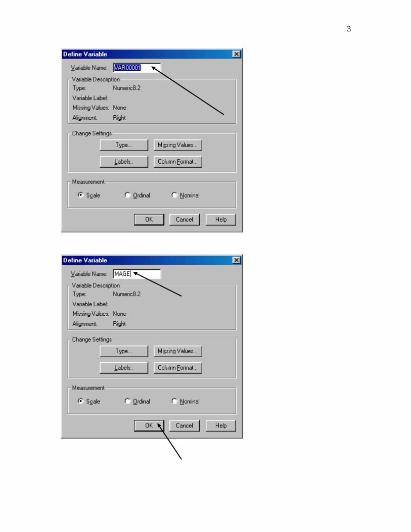
1 EDF 7405 Advanced Quantitative Methods in Educational Research DISC.SAS The data: Maternal Age Intelligence 15 69 16 105 17 79 18 108 19 105 20 94 21 91 22 107 23 114 24 105 25 112 Starting SPSS:
Transcript of Starting SPSS - University of Floridaplaza.ufl.edu/algina/all.part1.spss.pdf · This shows how to...

1
EDF 7405 Advanced Quantitative Methods in Educational Research
DISC.SAS
The data:
Maternal Age Intelligence
15 69 16 105 17 79 18 108 19 105 20 94 21 91 22 107 23 114 24 105 25 112
Starting SPSS:

2
Entering the data:
Please note that almost all screen shots in the directions for using SPSS are from SPSS 14. The appearance of these screen shots will be slightly different than the appearance of screen shots created from earlier or later versions of SPSS. An occasional a screen shot is from SPSS16.
3
4
5
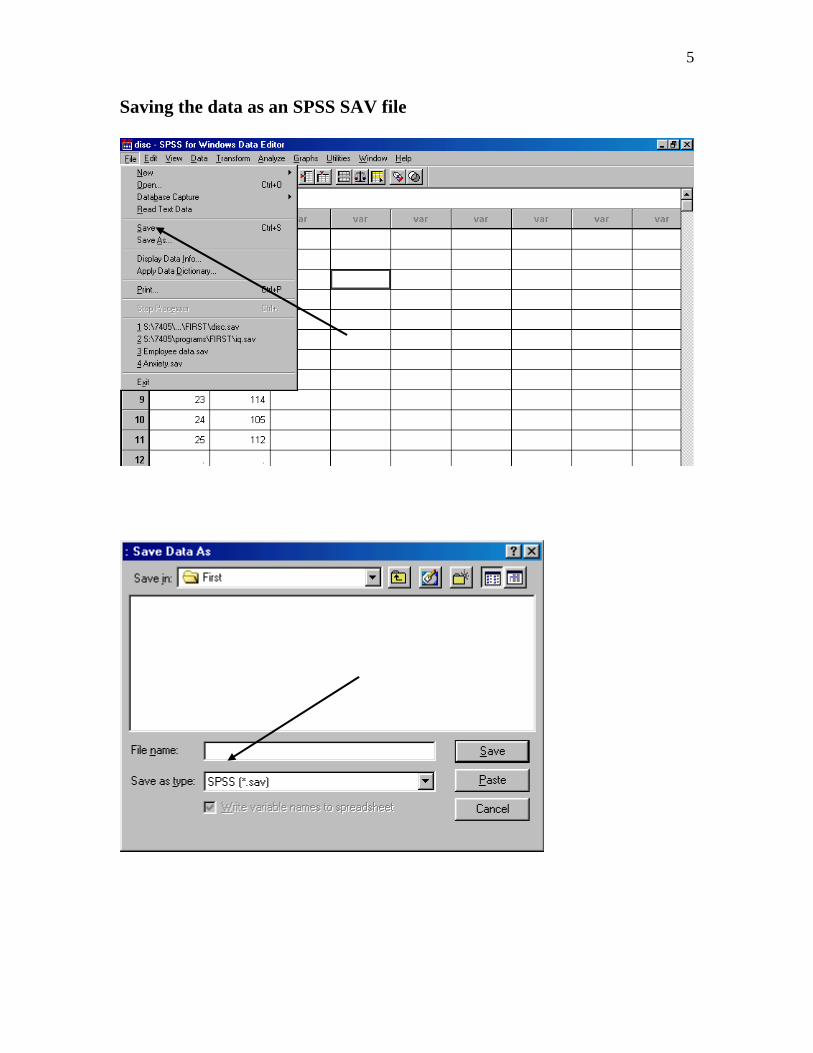
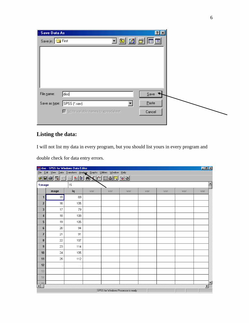
Saving the data as an SPSS SAV file
6
Listing the data: I will not list my data in every program, but you should list yours in every program and
double check for data entry errors.
7
8
9
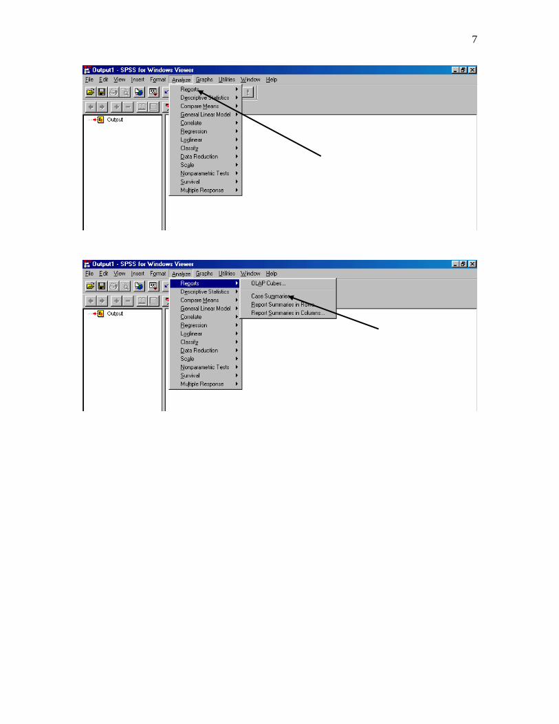
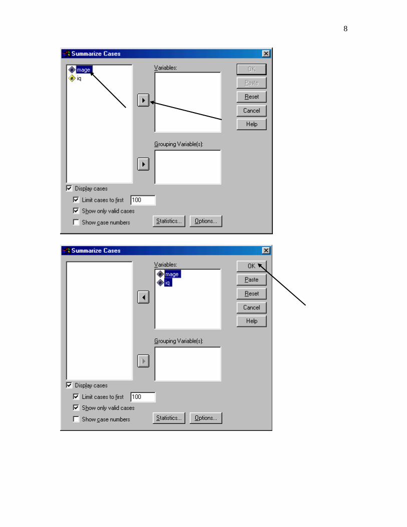
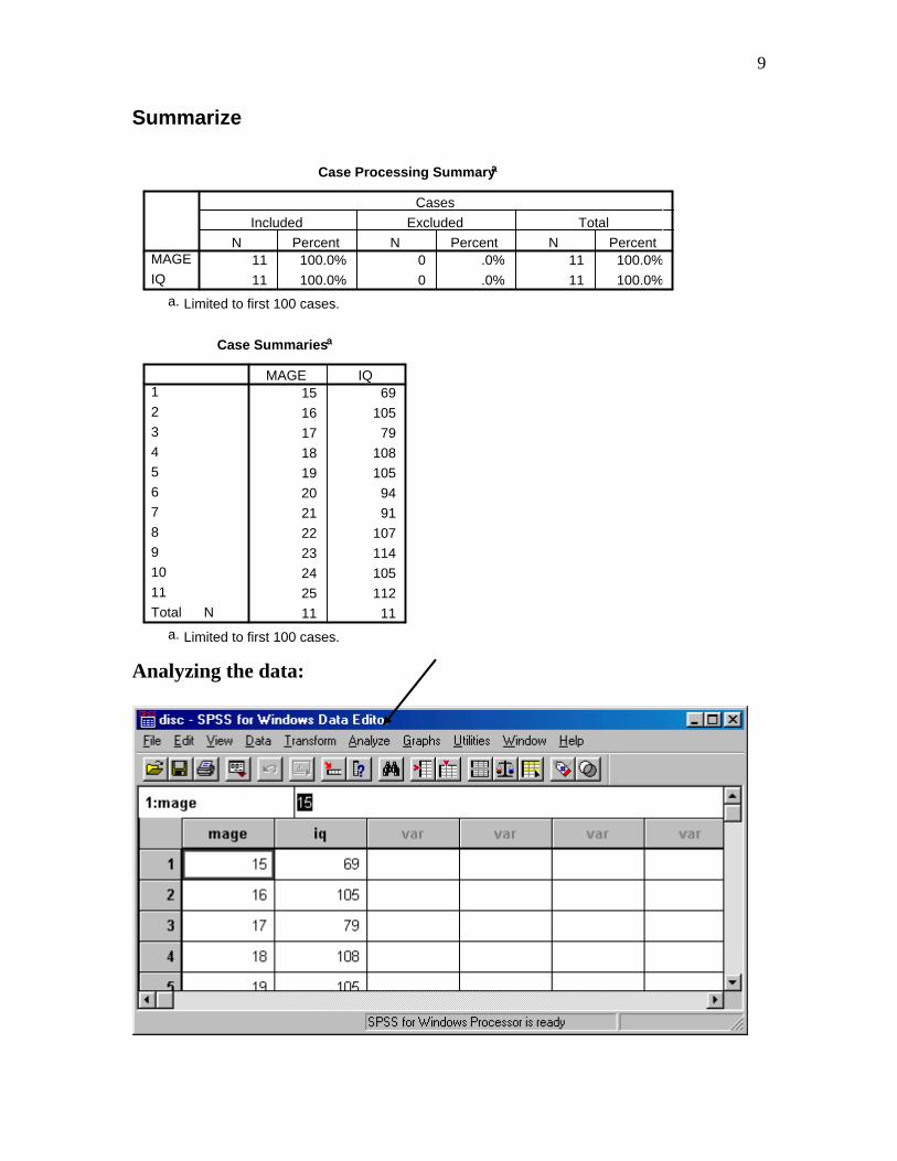
Summarize
Case Processing Summarya
11 100.0% 0 .0% 11 100.0%
11 100.0% 0 .0% 11 100.0%
MAGE
IQ
N Percent N Percent N Percent
Included Excluded Total
Cases
Limited to first 100 cases.a.
Case Summariesa
15 69
16 105
17 79
18 108
19 105
20 94
21 91
22 107
23 114
24 105
25 112
11 11
1
2
3
4
5
6
7
8
9
10
11
NTotal
MAGE IQ
Limited to first 100 cases.a.
Analyzing the data:
10
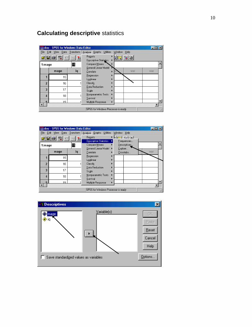
Calculating descriptive statistics
11
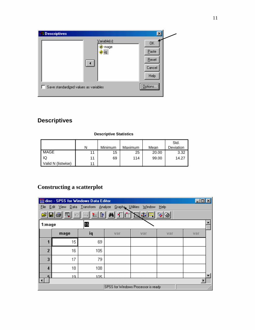
Descriptives
Descriptive Statistics
11 15 25 20.00 3.32
11 69 114 99.00 14.27
11
MAGE
IQ
Valid N (listwise)
N Minimum Maximum MeanStd.
Deviation
Constructing a scatterplot

12
This screen shot is from an older version of SPSS. With SPSS 15 or 16, select legacy diaglogs.
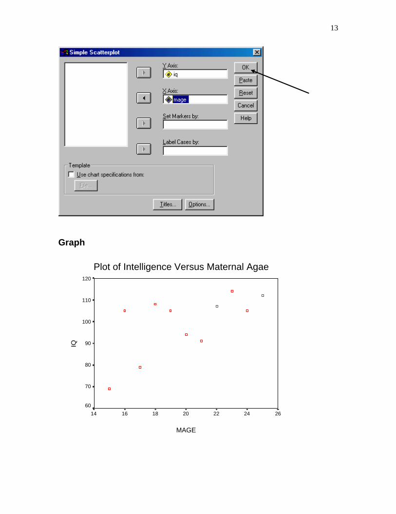
13
Graph
Plot of Intelligence Versus Maternal Agae
MAGE
26242220181614
IQ
120
110
100
90
80
70
60
14
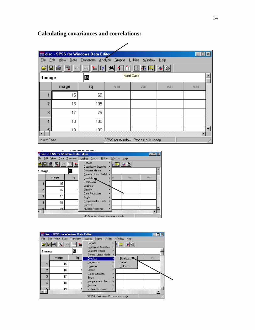
Calculating covariances and correlations:

15
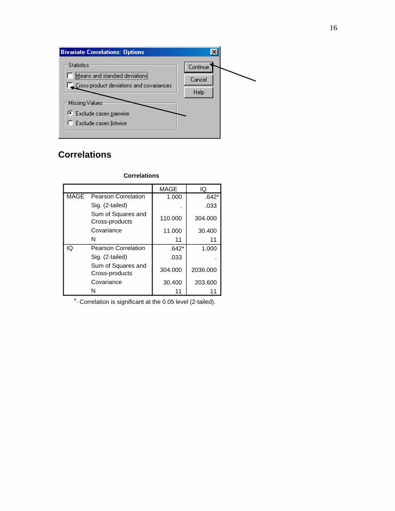
16
Correlations
Correlations
1.000 .642*
. .033
110.000 304.000
11.000 30.400
11 11
.642* 1.000
.033 .
304.000 2036.000
30.400 203.600
11 11
Pearson Correlation
Sig. (2-tailed)
Sum of Squares andCross-products
Covariance
N
Pearson Correlation
Sig. (2-tailed)
Sum of Squares andCross-products
Covariance
N
MAGE
IQ
MAGE IQ
Correlation is significant at the 0.05 level (2-tailed).*.
17
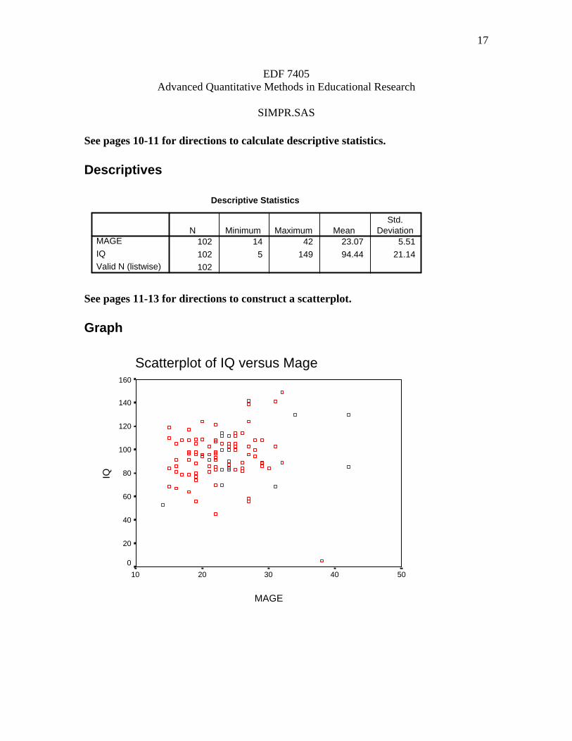
EDF 7405 Advanced Quantitative Methods in Educational Research
SIMPR.SAS
See pages 10-11 for directions to calculate descriptive statistics. Descriptives
Descriptive Statistics
102 14 42 23.07 5.51
102 5 149 94.44 21.14
102
MAGE
IQ
Valid N (listwise)
N Minimum Maximum MeanStd.
Deviation
See pages 11-13 for directions to construct a scatterplot. Graph
Scatterplot of IQ versus Mage
MAGE
5040302010
IQ
160
140
120
100
80
60
40
20
0
18
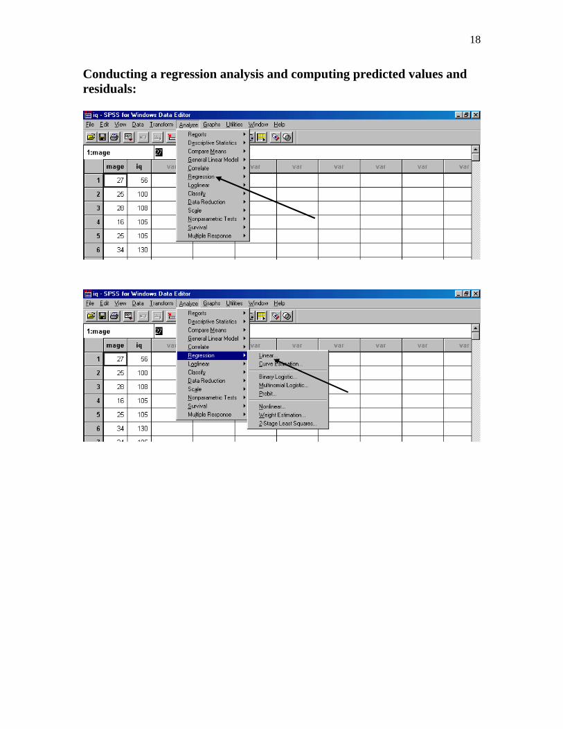
Conducting a regression analysis and computing predicted values and residuals:
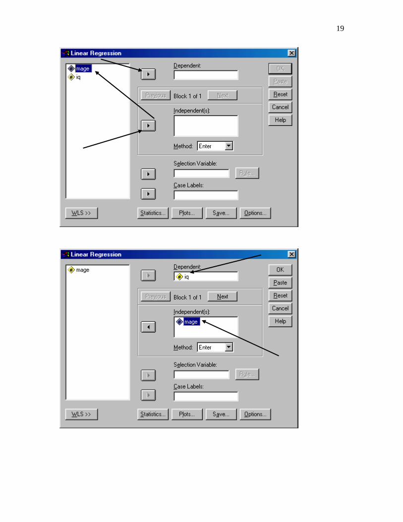
19
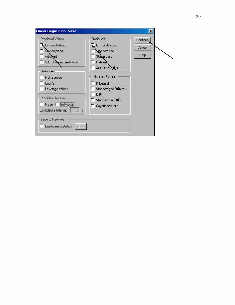
20
21
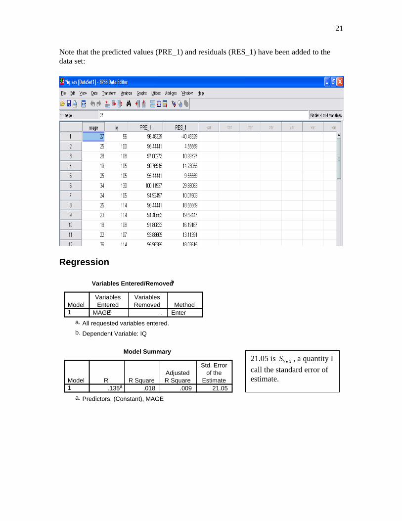
Note that the predicted values (PRE_1) and residuals (RES_1) have been added to the data set:
Regression
Variables Entered/Removedb
MAGEa . EnterModel1
VariablesEntered
VariablesRemoved Method
All requested variables entered.a.
Dependent Variable: IQb.
Model Summary
.135a .018 .009 21.05Model1
R R SquareAdjustedR Square
Std. Errorof the
Estimate
Predictors: (Constant), MAGEa.
21.05 is , a quantity I
call the standard error of estimate.
Y XS
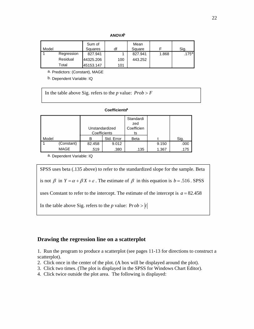
22
ANOVAb
827.941 1 827.941 1.868 .175a
44325.206 100 443.252
45153.147 101
Regression
Residual
Total
Model1
Sum ofSquares df
MeanSquare F Sig.
Predictors: (Constant), MAGEa.
Dependent Variable: IQb.
In the table above Sig. refers to the p value: Prob F
Coefficientsa
82.458 9.012 9.150 .000
.519 .380 .135 1.367 .175
(Constant)
MAGE
Model1
B Std. Error
UnstandardizedCoefficients
Beta
Standardized
Coefficients
t Sig.
Dependent Variable: IQa.
SPSS uses beta (.135 above) to refer to the standardized slope for the sample. Beta
is not in Y X . The estimate of in this equation is b .516 . SPSS
uses Constant to refer to the intercept. The estimate of the intercept is
In the table above Sig. refers to the p value:
82.458a
Pr ob t
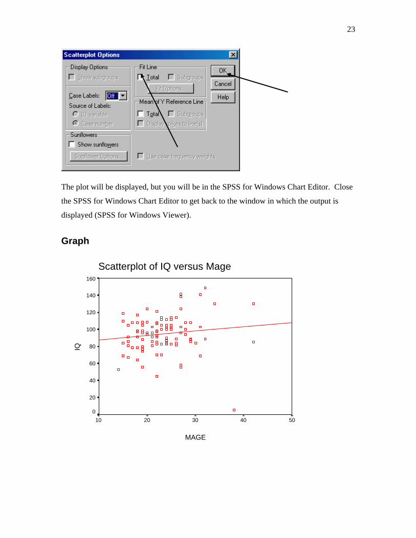
Drawing the regression line on a scatterplot
1. Run the program to produce a scatterplot (see pages 11-13 for directions to construct a scatterplot). 2. Click once in the center of the plot. (A box will be displayed around the plot). 3. Click two times. (The plot is displayed in the SPSS for Windows Chart Editor). 4. Click twice outside the plot area. The following is displayed:
23
The plot will be displayed, but you will be in the SPSS for Windows Chart Editor. Close
the SPSS for Windows Chart Editor to get back to the window in which the output is
displayed (SPSS for Windows Viewer).
Graph
Scatterplot of IQ versus Mage
MAGE
5040302010
IQ
160
140
120
100
80
60
40
20
0

24
25
EDF 7405 Advanced Quantitative Methods in Educational Research
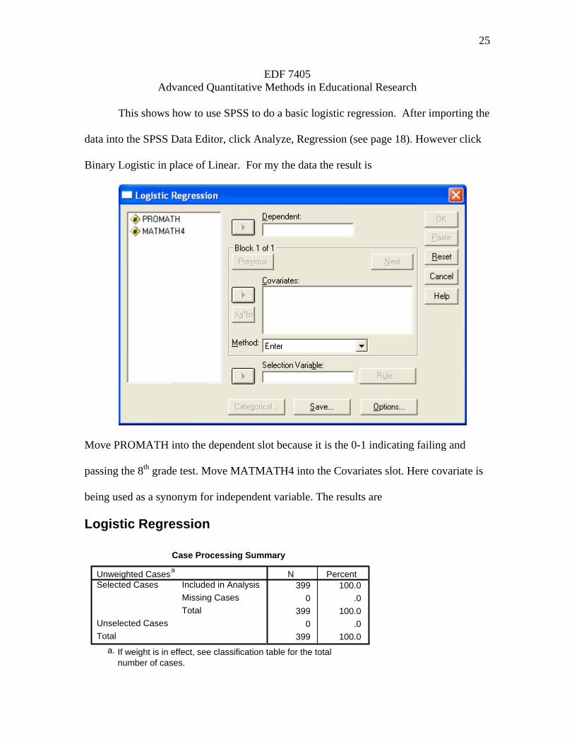
This shows how to use SPSS to do a basic logistic regression. After importing the
data into the SPSS Data Editor, click Analyze, Regression (see page 18). However click
Binary Logistic in place of Linear. For my the data the result is
Move PROMATH into the dependent slot because it is the 0-1 indicating failing and
passing the 8th grade test. Move MATMATH4 into the Covariates slot. Here covariate is
being used as a synonym for independent variable. The results are
Logistic Regression
Case Processing Summary
399 100.0
0 .0
399 100.0
0 .0
399 100.0
Unweighted Casesa
Included in Analysis
Missing Cases
Total
Selected Cases
Unselected Cases
Total
N Percent
If weight is in effect, see classification table for the totalnumber of cases.
a.
26
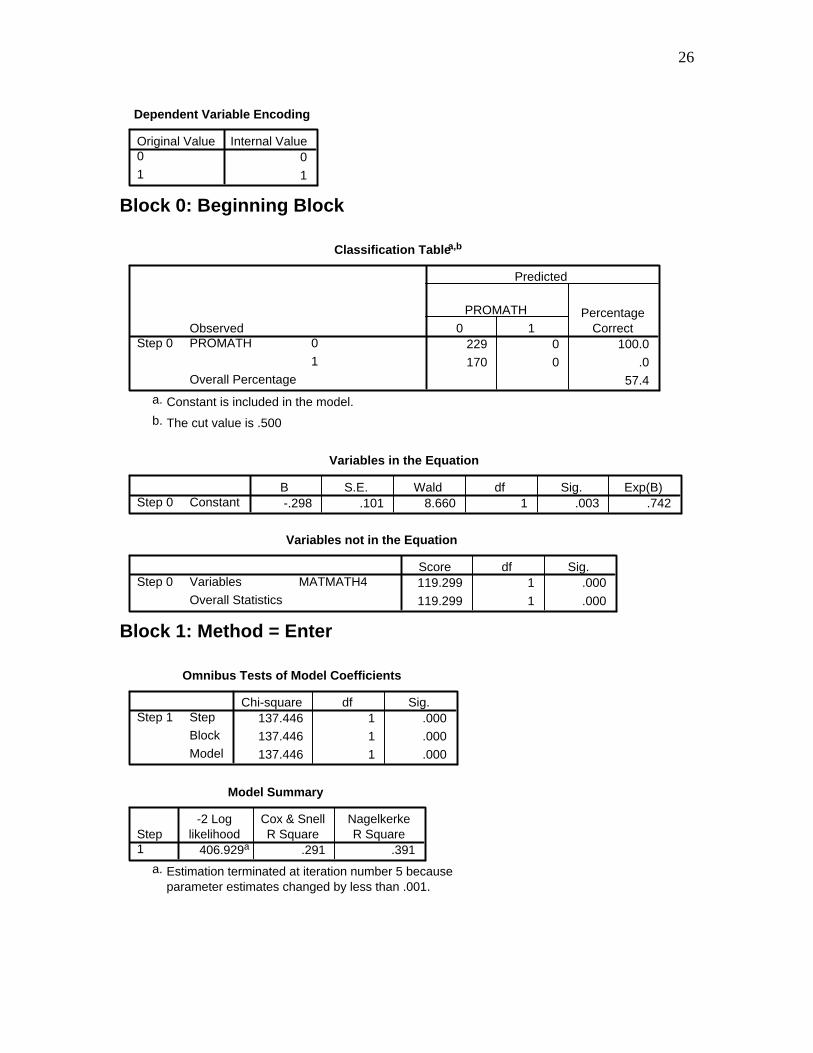
Dependent Variable Encoding
0
1
Original Value0
1
Internal Value
Block 0: Beginning Block
Classification Tablea,b
229 0 100.0
170 0 .0
57.4
Observed0
1
PROMATH
Overall Percentage
Step 00 1
PROMATH PercentageCorrect
Predicted
Constant is included in the model.a.
The cut value is .500b.
Variables in the Equation
-.298 .101 8.660 1 .003 .742ConstantStep 0B S.E. Wald df Sig. Exp(B)
Variables not in the Equation
119.299 1 .000
119.299 1 .000
MATMATH4Variables
Overall Statistics
Step 0Score df Sig.
Block 1: Method = Enter
Omnibus Tests of Model Coefficients
137.446 1 .000
137.446 1 .000
137.446 1 .000
Step
Block
Model
Step 1Chi-square df Sig.
Model Summary
406.929a .291 .391Step1
-2 Loglikelihood
Cox & SnellR Square
NagelkerkeR Square
Estimation terminated at iteration number 5 becauseparameter estimates changed by less than .001.
a.
27
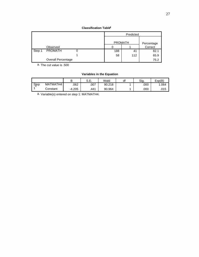
Classification Tablea
188 41 82.1
58 112 65.9
75.2
Observed0
1
PROMATH
Overall Percentage
Step 10 1
PROMATH PercentageCorrect
Predicted
The cut value is .500a.
Variables in the Equation
.062 .007 90.218 1 .000 1.064
-4.205 .441 90.964 1 .000 .015
MATMATH4
Constant
Step1
a
B S.E. Wald df Sig. Exp(B)
Variable(s) entered on step 1: MATMATH4.a.

28

29
EDF 7405 Advanced Quantitative Methods in Educational Research
HETERO.SAS
The variables in this example are the number of workers supervised 27 industrial
companies and the number of supervisors in the same companies. In the analysis number
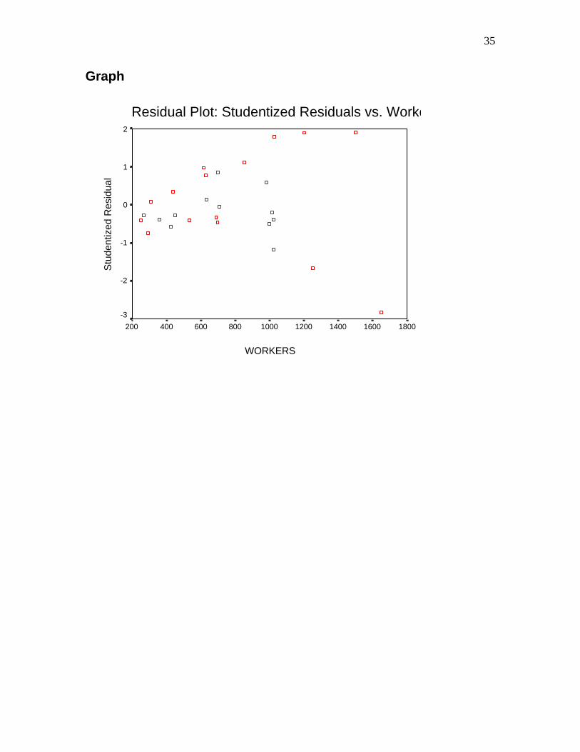
of supervisors is the dependent variable. The new feature of this program is a residual
plot. Residual plots are used to detect violations of assumptions,
The Data Workers Supervisors
294 30 247 32 267 37 358 44 423 47 311 49 450 56 534 62 438 68 697 78 688 80 630 84 709 88 627 97 615 100 999 109 1022 114 1015 117 700 106 850 128 980 130 1025 160 1021 97 1200 180 1250 112 1500 210 1650 135
30
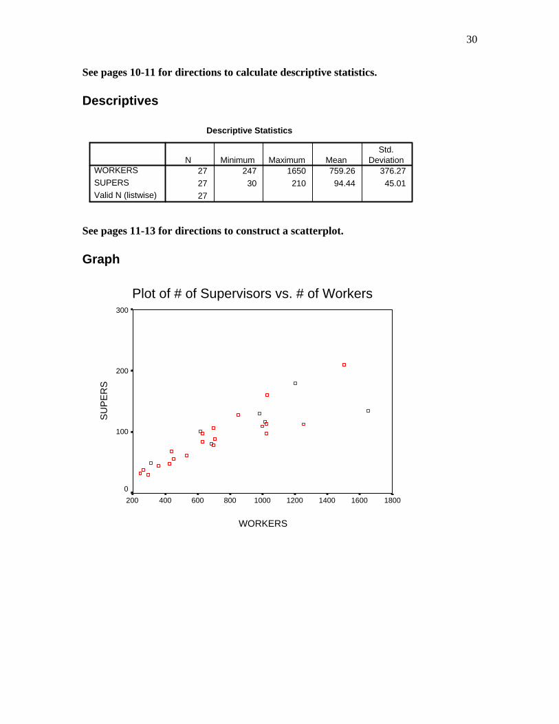
See pages 10-11 for directions to calculate descriptive statistics. Descriptives
Descriptive Statistics
27 247 1650 759.26 376.27
27 30 210 94.44 45.01
27
WORKERS
SUPERS
Valid N (listwise)
N Minimum Maximum MeanStd.
Deviation
See pages 11-13 for directions to construct a scatterplot. Graph
Plot of # of Supervisors vs. # of Workers
WORKERS
18001600140012001000800600400200
SU
PE
RS
300
200
100
0
31
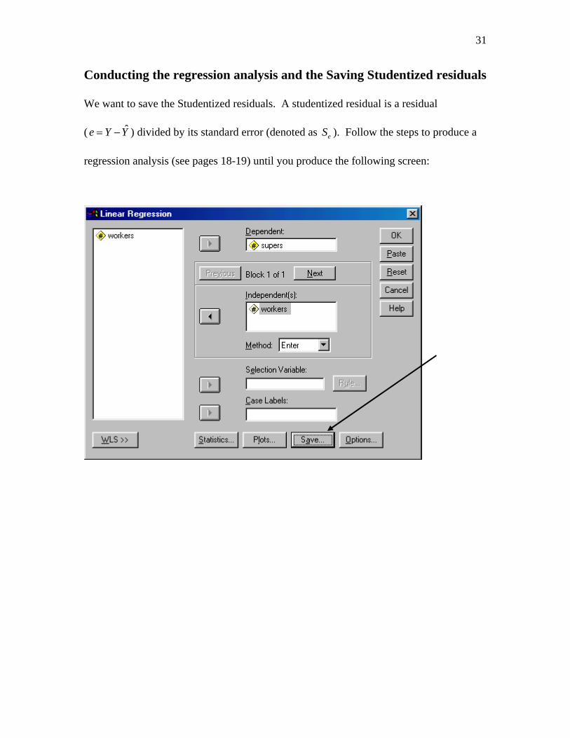
Conducting the regression analysis and the Saving Studentized residuals
We want to save the Studentized residuals. A studentized residual is a residual
( ) divided by its standard error (denoted as ). Follow the steps to produce a
regression analysis (see pages 18-19) until you produce the following screen:
ˆe Y Y eS

32
The following shows that the Studentized residuals have been added to the data set.
These are now available for plotting. If you want to, these can be saved for future work.
33
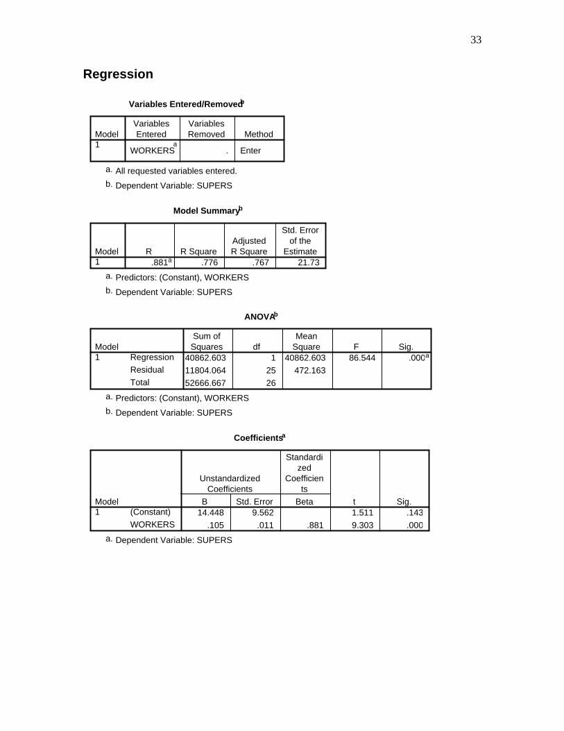
Regression
Variables Entered/Removedb
WORKERSa
. Enter
Model1
VariablesEntered
VariablesRemoved Method
All requested variables entered.a.
Dependent Variable: SUPERSb.
Model Summaryb
.881a .776 .767 21.73Model1
R R SquareAdjustedR Square
Std. Errorof the
Estimate
Predictors: (Constant), WORKERSa.
Dependent Variable: SUPERSb.
ANOVAb
40862.603 1 40862.603 86.544 .000a
11804.064 25 472.163
52666.667 26
Regression
Residual
Total
Model1
Sum ofSquares df
MeanSquare F Sig.
Predictors: (Constant), WORKERSa.
Dependent Variable: SUPERSb.
Coefficientsa
14.448 9.562 1.511 .143
.105 .011 .881 9.303 .000
(Constant)
WORKERS
Model1
B Std. Error
UnstandardizedCoefficients
Beta
Standardized
Coefficients
t Sig.
Dependent Variable: SUPERSa.
34
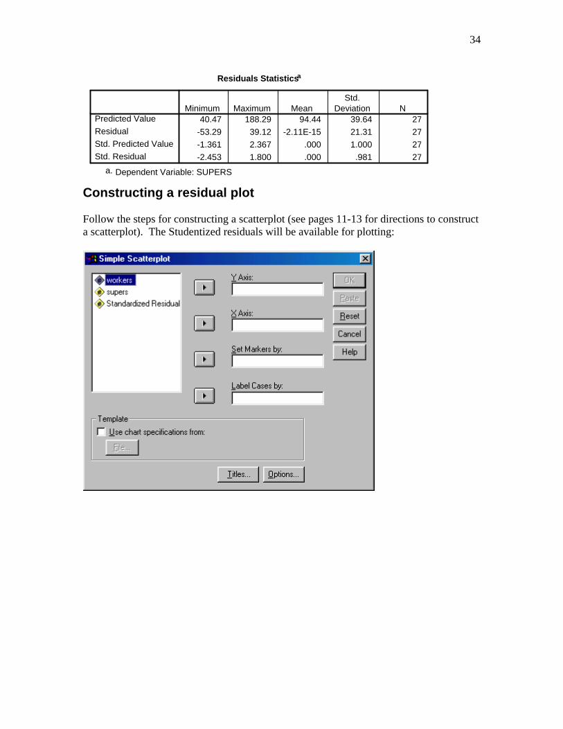
Residuals Statisticsa
40.47 188.29 94.44 39.64 27
-53.29 39.12 -2.11E-15 21.31 27
-1.361 2.367 .000 1.000 27
-2.453 1.800 .000 .981 27
Predicted Value
Residual
Std. Predicted Value
Std. Residual
Minimum Maximum MeanStd.
Deviation N
Dependent Variable: SUPERSa.
Constructing a residual plot Follow the steps for constructing a scatterplot (see pages 11-13 for directions to construct a scatterplot). The Studentized residuals will be available for plotting:
35
Graph
Residual Plot: Studentized Residuals vs. Worke
WORKERS
18001600140012001000800600400200
Stu
dent
ized
Res
idua
l
2
1
0
-1
-2
-3

36
37
EDF 7405 Advanced Quantitative Methods in Educational Research
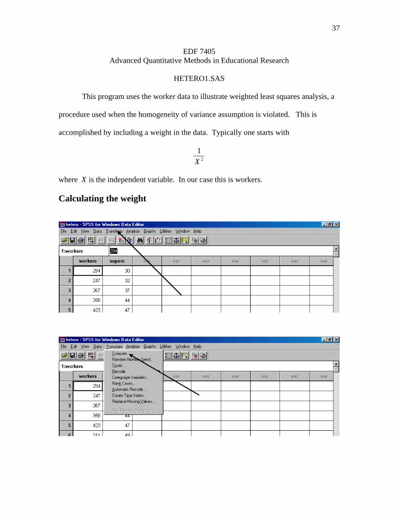
HETERO1.SAS
This program uses the worker data to illustrate weighted least squares analysis, a
procedure used when the homogeneity of variance assumption is violated. This is
accomplished by including a weight in the data. Typically one starts with
2
1
X
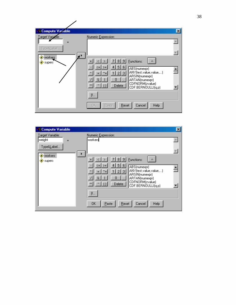
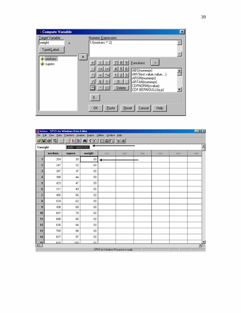
where X is the independent variable. In our case this is workers. Calculating the weight
38
39
40
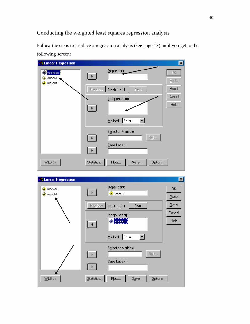
Conducting the weighted least squares regression analysis
Follow the steps to produce a regression analysis (see page 18) until you get to the
following screen:

41 41
42
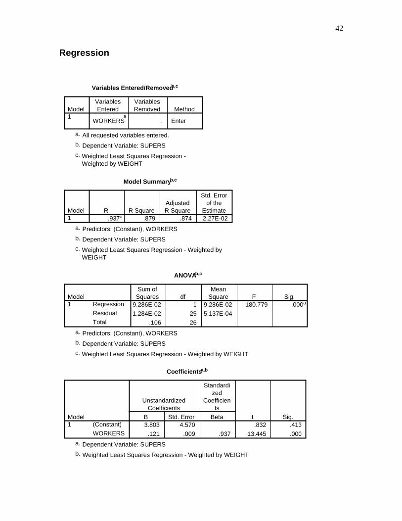
Regression
Variables Entered/Removedb,c
WORKERSa
. Enter
Model1
VariablesEntered
VariablesRemoved Method
All requested variables entered.a.
Dependent Variable: SUPERSb.
Weighted Least Squares Regression -Weighted by WEIGHT
c.
Model Summaryb,c
.937a .879 .874 2.27E-02Model1
R R SquareAdjustedR Square
Std. Errorof the
Estimate
Predictors: (Constant), WORKERSa.
Dependent Variable: SUPERSb.
Weighted Least Squares Regression - Weighted byWEIGHT
c.
ANOVAb,c
9.286E-02 1 9.286E-02 180.779 .000a
1.284E-02 25 5.137E-04
.106 26
Regression
Residual
Total
Model1
Sum ofSquares df
MeanSquare F Sig.
Predictors: (Constant), WORKERSa.
Dependent Variable: SUPERSb.
Weighted Least Squares Regression - Weighted by WEIGHTc.
Coefficientsa,b
3.803 4.570 .832 .413
.121 .009 .937 13.445 .000
(Constant)
WORKERS
Model1
B Std. Error
UnstandardizedCoefficients
Beta
Standardized
Coefficients
t Sig.
Dependent Variable: SUPERSa.
Weighted Least Squares Regression - Weighted by WEIGHTb.
43
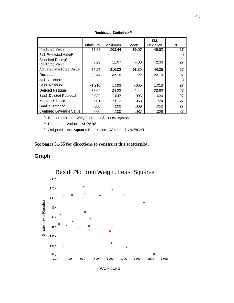
Residuals Statisticsb,c
33.69 203.44 95.67 45.52 27
. . . . 0
2.22 11.07 4.30 2.38 27
34.27 210.02 95.89 46.05 27
-68.44 32.18 -1.22 22.10 27
. . . . 0
-1.916 1.593 -.005 1.018 27
-75.02 34.23 -1.44 23.82 27
-2.032 1.647 -.006 1.039 27
.001 2.612 .963 .724 27
.000 .208 .039 .052 27
.000 .100 .037 .028 27
Predicted Value
Std. Predicted Valuea
Standard Error ofPredicted Value
Adjusted Predicted Value
Residual
Std. Residuala
Stud. Residual
Deleted Residual
Stud. Deleted Residual
Mahal. Distance
Cook's Distance
Centered Leverage Value
Minimum Maximum MeanStd.
Deviation N
Not computed for Weighted Least Squares regression.a.
Dependent Variable: SUPERSb.
Weighted Least Squares Regression - Weighted by WEIGHTc.
See pages 31-35 for directions to construct this scatterplot. Graph
Resid. Plot from Weight. Least Squares
WORKERS
18001600140012001000800600400200
Stu
dent
ized
Res
idua
l
2.0
1.5
1.0
.5
0.0
-.5
-1.0
-1.5
-2.0

44
45
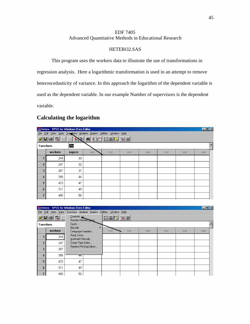
EDF 7405 Advanced Quantitative Methods in Educational Research
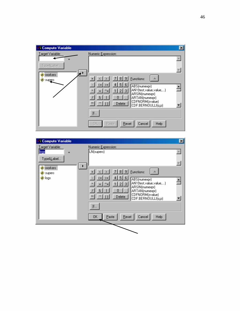
HETERO2.SAS
This program uses the workers data to illustrate the use of transformations in
regression analysis. Here a logarithmic transformation is used in an attempt to remove
heteroscedasticity of variance. In this approach the logarithm of the dependent variable is
used as the dependent variable. In our example Number of supervisors is the dependent
variable.
Calculating the logarithm
46
47
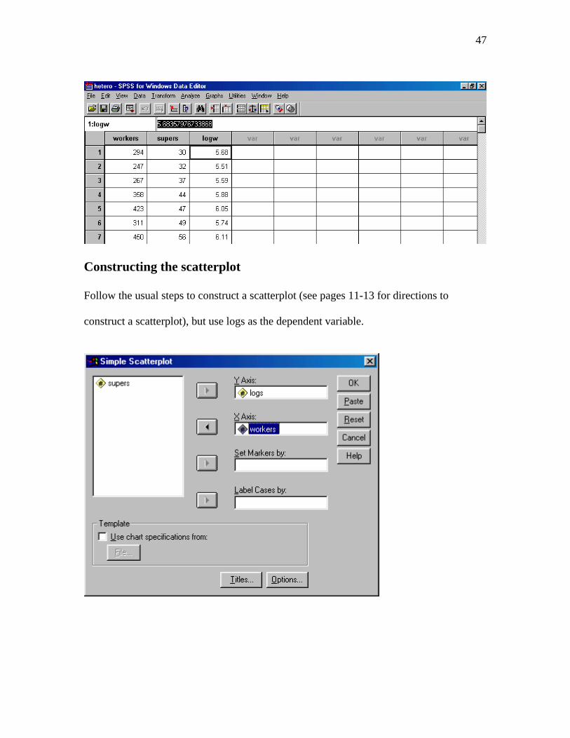
Constructing the scatterplot Follow the usual steps to construct a scatterplot (see pages 11-13 for directions to
construct a scatterplot), but use logs as the dependent variable.

48
Graph
WORKERS
18001600140012001000800600400200
LOG
S5.5
5.0
4.5
4.0
3.5
3.0
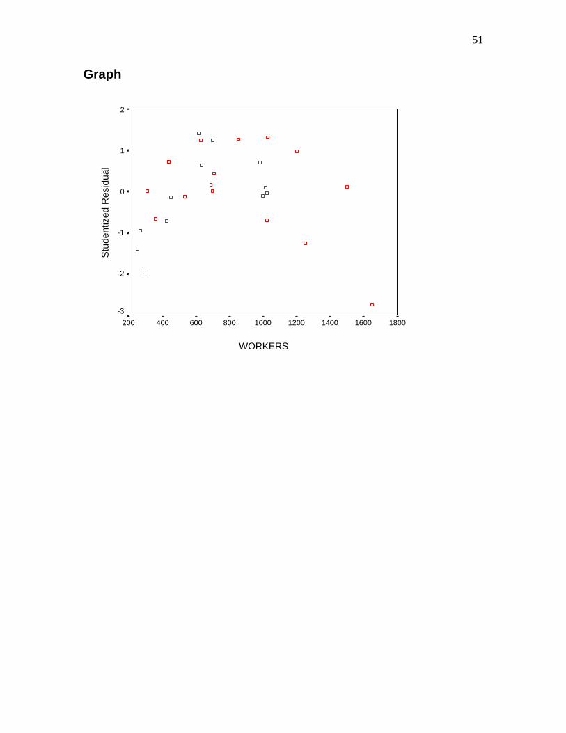
Conducting the regression analysis Follow the usual steps to conduct the regression analysis but use logs as the dependent
variable. As usual save the Studentized residuals.

49
Regression
Variables Entered/Removedb
WORKERSa
. Enter
Model1
VariablesEntered
VariablesRemoved Method
All requested variables entered.a.
Dependent Variable: LOGSb.
Model Summaryb
.878a .770 .761 .2524Model1
R R SquareAdjustedR Square
Std. Errorof the
Estimate
Predictors: (Constant), WORKERSa.
Dependent Variable: LOGSb.
50
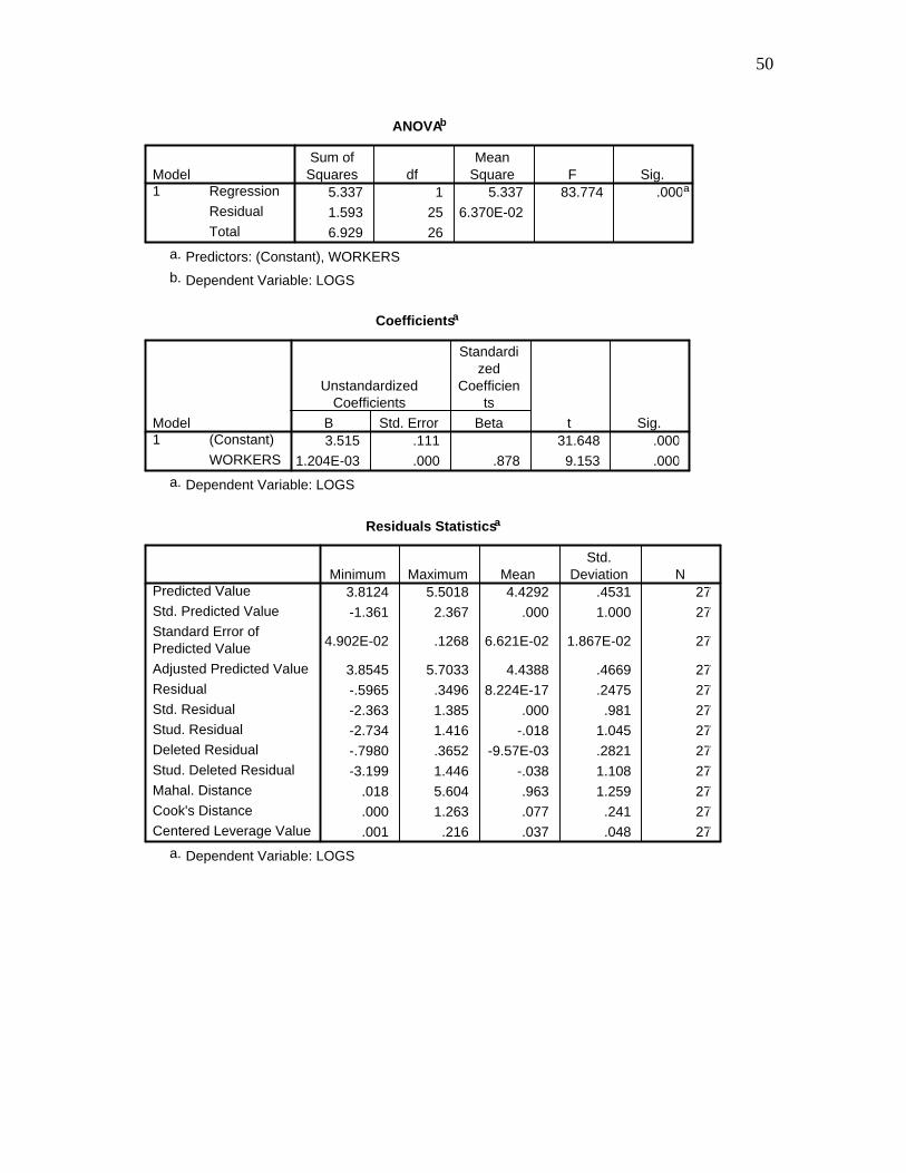
ANOVAb
5.337 1 5.337 83.774 .000a
1.593 25 6.370E-02
6.929 26
Regression
Residual
Total
Model1
Sum ofSquares df
MeanSquare F Sig.
Predictors: (Constant), WORKERSa.
Dependent Variable: LOGSb.
Coefficientsa
3.515 .111 31.648 .000
1.204E-03 .000 .878 9.153 .000
(Constant)
WORKERS
Model1
B Std. Error
UnstandardizedCoefficients
Beta
Standardized
Coefficients
t Sig.
Dependent Variable: LOGSa.
Residuals Statisticsa
3.8124 5.5018 4.4292 .4531 27
-1.361 2.367 .000 1.000 27
4.902E-02 .1268 6.621E-02 1.867E-02 27
3.8545 5.7033 4.4388 .4669 27
-.5965 .3496 8.224E-17 .2475 27
-2.363 1.385 .000 .981 27
-2.734 1.416 -.018 1.045 27
-.7980 .3652 -9.57E-03 .2821 27
-3.199 1.446 -.038 1.108 27
.018 5.604 .963 1.259 27
.000 1.263 .077 .241 27
.001 .216 .037 .048 27
Predicted Value
Std. Predicted Value
Standard Error ofPredicted Value
Adjusted Predicted Value
Residual
Std. Residual
Stud. Residual
Deleted Residual
Stud. Deleted Residual
Mahal. Distance
Cook's Distance
Centered Leverage Value
Minimum Maximum MeanStd.
Deviation N
Dependent Variable: LOGSa.
51
Graph
WORKERS
18001600140012001000800600400200
Stu
dent
ized
Res
idua
l2
1
0
-1
-2
-3