Reduced Model Results - University of Floridaplaza.ufl.edu/algina/all.part3.spss.pdf · 5.950E-03...

1

EDF 7405 Advanced Quantitative Methods in Educational Research

Data are available on IQ of the child and seven potential predictors. Four are

medical variables available at the birth of the child:

Birthweight (BW)—the weight of the new born in grams; very large or very small

weights may indicate health problems ( 1X ).

APGAR—a quick assessment of overall newborn well being. Low numbers may

indicate problems ( 2X ).

Intrapartum factors (IF) —a measure of the quality of the delivery. Low numbers

indicate problems occurred in the delivery ( 3X ).

Neonatal factors (NF)—a measure of the health of the newborn. Low numbers

may indicate health problems ( 4X ).

Three are sociological variables measured at the time of the baby’s birth.

Socioeconomic status—a measure of the material resources available to the

mother. Higher scores indicate more resources ( 5X ).

Social support—a measure of the social resources available to the mother. Higher

scores indicate more resources ( 6X ).

Stressful life events (SLE)—a measure of the extent of stressors in the mother’s

life in the prior year. Higher scores indicate more stressors ( 7X )

We want to consider the medical variables as control variables and test whether or

not the sociological variables are related to IQ when the medical variables are controlled.

To do this we need results for two models:

2

The full model:

1 1 2 2 3 3 4 4 5 5 6 6 7 7Y X X X X X X X

The reduced model:

1 1 2 2 3 3 4 4Y X X X X

In terms of the abbreviations for the variables these models are

The full model:

1 2 3 4 5 6 7Y BW APGAR IF NF SES SS SLE

The reduced model:

1 2 3 4Y BW APGAR IF NF

I present the regression results only. The residual plots for the full model should

be examined before using the results for the models.

Full Model Results See pages 18-19 of the first section for directions to conduct a regression analysis. Regression

Variables Entered/Removedb

SLE, IF,BW, SES,APGAR,SS, NF

a. Enter

Model1

VariablesEntered

VariablesRemoved Method

All requested variables entered.a.

Dependent Variable: IQb.

3

Model Summary

.601a .361 .312 16.13Model1

R R SquareAdjustedR Square

Std. Errorof the

Estimate

Predictors: (Constant), SLE, IF, BW, SES, APGAR,SS, NF

a.

ANOVAb

13380.436 7 1911.491 7.344 .000a

23686.069 91 260.286

37066.505 98

Regression

Residual

Total

Model1

Sum ofSquares df

MeanSquare F Sig.

Predictors: (Constant), SLE, IF, BW, SES, APGAR, SS, NFa.


Coefficientsa

33.085 16.709 1.980 .051

5.950E-03 .002 .274 2.569 .012

1.680 1.215 .143 1.382 .170

-.148 .186 -.070 -.795 .429

8.393E-02 .164 .062 .513 .609

2.255 .490 .450 4.607 .000

-.208 .366 -.061 -.570 .570

.268 .257 .097 1.041 .301

(Constant)

BW

APGAR

IF

NF

SES

SS

SLE

Model1

B Std. Error

UnstandardizedCoefficients

Beta

Standardized

Coefficients

t Sig.

Dependent Variable: IQa.

Reduced Model Results

4

See pages 18-19 of the first section for directions to conduct a regression analysis. Regression


NF, IF,APGAR,BW

a . Enter

Model1

VariablesEntered




Model Summary

.380a .144 .108 18.37Model1


Std. Errorof the

Estimate

Predictors: (Constant), NF, IF, APGAR, BWa.

ANOVAb

5347.170 4 1336.793 3.962 .005a

31719.335 94 337.440

37066.505 98

Regression

Residual

Total

Model1

Sum ofSquares df

MeanSquare F Sig.

Predictors: (Constant), NF, IF, APGAR, BWa.


Coefficientsa

55.691 15.559 3.579 .001

5.979E-03 .003 .276 2.366 .020

2.775 1.352 .236 2.053 .043

-.191 .210 -.090 -.908 .366

.125 .180 .093 .695 .489

(Constant)

BW

APGAR

IF

NF

Model1

B Std. Error


Beta

Standardized

Coefficients

t Sig.

Dependent Variable: IQa.

5


SEQUENT.SAS

In this handout a procedure for obtaining control-preceding variables tests is

presented. Here is the SPSS Windows editor with part of the data displayed.

To conduct the analysis press analyze, regression and linear

6

You get the following screen:

7

Move iq into the Dependent slot by highlighting iq and pressing the arrow to the left of

the Dependent slot and bw into the Independent(s) slot by highlighting bw and pressing

the arrow to the left of the independents slot. You get

Now press next. You get

8

Notice that Block 1 of 1 has changed to Block 2 of 2 and the Independent(s) slot is

empty. Move SES into the Independent(s) slot. You get

Press next. You get

9

Notice that Block 2 of 2 has changed to Block 3 of 3 and the Independent(s) slot is

empty. Move MAGE in the Independent(s) slot. Continue in this fashion until you have

moved all independent variables into the Independent(s) and in the appropriate order. The

final screen looks like this

10

Block 8 of 8 indicates that eight independent variables have been moved to the

Independent(s) slot.

Now click Statistics. The screen looks like this

Unclick estimates and click R squared change. Then click continue and when the new

screen opens, click OK.

These results follow over several pages.

Regression [DataSet1] C:\7405\Spss.Programs\Third\sequent.sav


bwa . Enter

ses a . Enter

magea . Enter

apgara . Enter

nfa . Enter

ifa . Enter

ss a . Enter

slea . Enter

Model1

2

3

4

5

6

7

8

VariablesEntered



Dependent Variable: iqb.

11

In the following you will find the 2 up to jR X in the R square column, the Type I squared semi partial correlation coefficients in

the R square change column, the control-preceding-variables F statistic in the F change column and the control-preceding-

variables p value in the Sig F change column.

Model Summary

.302a .091 .082 18.636 .091 9.726 1 97 .002

.575b .330 .316 16.082 .239 34.252 1 96 .000

.576c .332 .311 16.145 .002 .252 1 95 .617

.589d .347 .319 16.044 .015 2.204 1 94 .141

.591e .349 .314 16.109 .002 .247 1 93 .620

.595f .354 .312 16.132 .005 .730 1 92 .395

.595g .354 .305 16.218 .000 .024 1 91 .877

.602h .362 .306 16.207 .008 1.124 1 90 .292

Model1

2

3

4

5

6

7

8


Std. Error ofthe Estimate

R SquareChange F Change df1 df2 Sig. F Change

Change Statistics

Predictors: (Constant), bwa.

Predictors: (Constant), bw, sesb.

Predictors: (Constant), bw, ses, magec.

Predictors: (Constant), bw, ses, mage, apgard.

Predictors: (Constant), bw, ses, mage, apgar, nfe.

Predictors: (Constant), bw, ses, mage, apgar, nf, iff.

Predictors: (Constant), bw, ses, mage, apgar, nf, if, ssg.

Predictors: (Constant), bw, ses, mage, apgar, nf, if, ss, sleh.

12

The following results contain the F statistics for testing the omnibus multivariable

hypothesis for each successive model. We do not use these results.

ANOVAi

3377.765 1 3377.765 9.726 .002a

33688.740 97 347.307

37066.505 98

12236.756 2 6118.378 23.656 .000b

24829.749 96 258.643

37066.505 98

12302.426 3 4100.809 15.732 .000c

24764.079 95 260.675

37066.505 98

12869.711 4 3217.428 12.499 .000d

24196.794 94 257.413

37066.505 98

12933.774 5 2586.755 9.969 .000e

24132.732 93 259.492

37066.505 98

13123.628 6 2187.271 8.405 .000f

23942.877 92 260.249

37066.505 98

13129.957 7 1875.708 7.131 .000g

23936.548 91 263.039

37066.505 98

13425.298 8 1678.162 6.389 .000h

23641.207 90 262.680

37066.505 98

Regression

Residual

Total

Regression

Residual

Total

Regression

Residual

Total

Regression

Residual

Total

Regression

Residual

Total

Regression

Residual

Total

Regression

Residual

Total

Regression

Residual

Total

Model1

2

3

4

5

6

7

8

Sum ofSquares df Mean Square F Sig.

Predictors: (Constant), bwa.

Predictors: (Constant), bw, sesb.

Predictors: (Constant), bw, ses, magec.

Predictors: (Constant), bw, ses, mage, apgard.

Predictors: (Constant), bw, ses, mage, apgar, nfe.

Predictors: (Constant), bw, ses, mage, apgar, nf, iff.

Predictors: (Constant), bw, ses, mage, apgar, nf, if, ssg.

Predictors: (Constant), bw, ses, mage, apgar, nf, if, ss, sleh.

Dependent Variable: iqi.

13


Fathers are randomly assigned to either an experimental or a control group. The

experimental treatment is designed to increase fathers' authoritative towards child rearing.

The fathers were post tested with the Eversoll Father Role Questionnaire. In the data the

control group is coded

1Z for the experimental group

0Z for the control group

This kind of coding is called dummy coding. The variable is denoted by a Z to emphasize that it is a categorical variable rather than a quantitative variable.

14

The Data

Group EFRQ 0 97 0 112 0 112 0 94 0 111 0 85 0 108 0 107 0 111 0 86 0 103 0 92 0 120 1 112 1 109 1 97 1 95 1 103 1 104 1 118 1 107 1 115 1 94 1 100 1 90 1 108

The model is

Y Z

or in terms of the abbreviations for the variables EFRQ Group

The symbol is used in place of to emphasize that it is a regression coefficient for a categorical variable rather than for a quantitative variable.

15

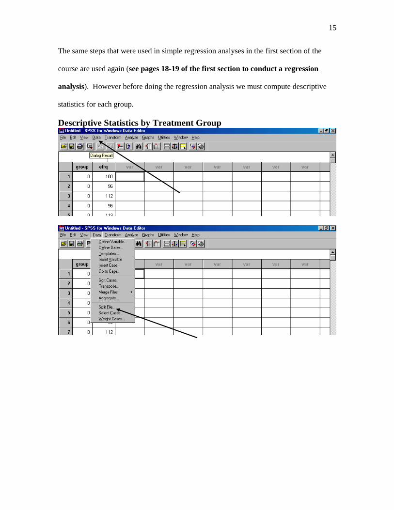
The same steps that were used in simple regression analyses in the first section of the

course are used again (see pages 18-19 of the first section to conduct a regression

analysis). However before doing the regression analysis we must compute descriptive

statistics for each group.

Descriptive Statistics by Treatment Group

16

See pages 10-11 of the first section for directions to obtain descriptive statistics.

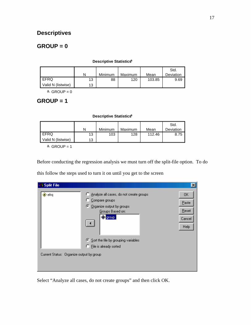
17

Descriptives GROUP = 0

Descriptive Statisticsa

13 88 120 103.85 9.69

13

EFRQ

Valid N (listwise)

N Minimum Maximum MeanStd.

Deviation

GROUP = 0a.

GROUP = 1


13 103 128 112.46 8.75

13

EFRQ

Valid N (listwise)


Deviation

GROUP = 1a.

Before conducting the regression analysis we must turn off the split-file option. To do

this follow the steps used to turn it on until you get to the screen

Select “Analyze all cases, do not create groups” and then click OK.

18

Regression Analysis Regression


GROUPa . EnterModel1

VariablesEntered



Dependent Variable: EFRQb.

Model Summary

.437a .191 .157 9.24Model1


Std. Errorof the

Estimate

Predictors: (Constant), GROUPa.

ANOVAb

482.462 1 482.462 5.657 .026a

2046.923 24 85.288

2529.385 25

Regression

Residual

Total

Model1

Sum ofSquares df

MeanSquare F Sig.

Predictors: (Constant), GROUPa.

Dependent Variable: EFRQb.

Coefficientsa

103.846 2.561 40.543 .000

8.615 3.622 .437 2.378 .026

(Constant)

GROUP

Model1

B Std. Error


Beta

Standardized

Coefficients

t Sig.

Dependent Variable: EFRQa.

19


QUAL1.SAS

Data are available on 51 teenage mothers and their children. The data consist of

dummy variables indicating the prenatal care program in which the mother took part and

mental development index (MDI) scores derived from the Bayley scales of infant

development. The prenatal care was delivered by the teenage pregnancy team, private

physicians, or the Shands’ high risk clinic. The coding of the groups is presented in the

following table

Prenatal Care 1Z 2Z

Teenage Pregnancy Team 1 0

Private Physician 0 1

Shands’ High Risk Clinic 0 0

The MDI scores were obtained at age six months. The data are used to illustrate the use

of regression to conduct a one-way between-subjects ANOVA.

Descriptive Statistics for Each Group

To get descriptive statistics on the groups, before using the Descriptive Statistics

option within the Analyze option it is necessary to split the file. To review, splitting the

file is done by using the Split File option within the Data option in the SPSS for

Windows Data Editor.

21

Descriptives Z1 = 0, Z2 = 0


13 91 152 118.38 21.13

13

MDI

Valid N (listwise)


Deviation

Z1 = 0, Z2 = 0a.

Z1 = 0, Z2 = 1


19 88 155 134.37 16.55

19

MDI

Valid N (listwise)


Deviation

Z1 = 0, Z2 = 1a.

Z1 = 1, Z2 = 0

22


19 94 144 120.84 14.74

19

MDI

Valid N (listwise)


Deviation

Z1 = 1, Z2 = 0a.

Before running the regression analysis the file must be unsplit. Just select Analyze all

cases, do not select groups in the following screen:

Regression Analysis The following is the result of running the SPSS regression analysis (see pages 18-19 of

the first section to conduct a regression analysis). It provided the test of the omnibus

hypothesis and of the comparison of Teenage Pregnancy Team to Shands’ High Risk

Clinic and of Private Physicians to Shands’ High Risk Clinic. A method for obtaining the

comparison of Teenage Pregnancy Team and Private Physicians is presented after the

initial regression results.

23

Regression


Z2, Z1a . EnterModel1

VariablesEntered



Dependent Variable: MDIb.

Model Summary

.391a .153 .118 17.20Model1


Std. Errorof the

Estimate

Predictors: (Constant), Z2, Z1a.

ANOVAb

2561.662 2 1280.831 4.329 .019a

14202.024 48 295.876

16763.686 50

Regression

Residual

Total

Model1

Sum ofSquares df

MeanSquare F Sig.

Predictors: (Constant), Z2, Z1a.

Dependent Variable: MDIb.

Coefficientsa

118.385 4.771 24.815 .000

2.457 6.191 .066 .397 .693

15.984 6.191 .426 2.582 .013

(Constant)

Z1

Z2

Model1

B Std. Error


Beta

Standardized

Coefficients

t Sig.

Dependent Variable: MDIa.

24

Unfortunately the SPSS regression program does not automatically produce a t

statistic for comparing Teenage Pregnancy Team and Private Physicians. The t statistic

can be computed by using the SPSS line code. In the following screen for the regression

program press Paste:

The SPSS syntax editor displays the following code: REGRESSION /MISSING LISTWISE /STATISTICS COEFF OUTS R ANOVA /CRITERIA=PIN(.05) POUT(.10) /NOORIGIN /DEPENDENT mdi /METHOD=ENTER z1 z2 Add BCOV to the statistics line:

REGRESSION /MISSING LISTWISE /STATISTICS COEFF OUTS R ANOVA BCOV /CRITERIA=PIN(.05) POUT(.10) /NOORIGIN

25

/DEPENDENT mdi /METHOD=ENTER z1 z2 Press Run and then press All. The results will be the same as for the new full model with

the exception that the following results will be added at the end.

Coefficient Correlations(a)

Model z2 z1 z2 1.000 .594Correlations

z1 .594 1.000z2 38.332 22.760

1

Covariances

z1 22.760 38.332

a Dependent Variable: mdi

These results are confusingly labeled because they are not correlation coefficients and

covariances for the variables. Rather they are sampling correlations and covariances.

The t statistic for 0 1 2: 0H is

1 2 1

1 2

2 2 2t

S S C2

The results required for the denominator are

Name of Statistic

Symbol Numeric value

Sampling variance for

1

1

2S

38.332


2

2

2S

38.332

Sampling covariance for

1 and 2

1 2

C

22.760

Each sampling variance is the square of a standard error, a term with which you are more

familiar. The coefficients 1 and 2 can be found in the results labeled coefficients.

These results are on page 23. Substituting in the t statistic for testing 0 1 2: 0H

26

1 2 1

1 2

2 2 2t

S S C2

yields

2.457 15.984

38.322 38.222 2 22.760

13.5272.42

31.124

27


ANCORAN1.SAS

In the investigation of the treatment designed to increase fathers' authoritative

towards child rearing, fathers were pre and post tested with the Eversoll Father Role

Questionnaire. This handout illustrates how to incorporate the pretest and test for the

covariate x treatment interaction. The groups are again coded



The data

Group EFPOST EFPRE 0 100 97 0 96 112 0 112 112 0 96 94 0 113 111 0 92 85 0 112 108 0 113 107 0 102 111 0 88 86 0 107 103 0 99 92 0 120 120 1 103 112 1 113 109 1 118 97 1 112 95 1 103 103 1 103 104 1 124 118 1 116 107 1 108 115 1 107 94 1 123 100 1 104 90 1 128 108

28

Model for testing the interaction:

The model is

Y X XZ

or in terms of the abbreviations of the variables ( ) ( )EFPOST EFPRE Group Group EFPRE .

The symbol emphasizes it is a regression coefficient for the product term.

We must use the TRANSFORM and COMPUTE option to add the product

to the data set (see pages 37-39 of the first section to use the

compute feature). The product is denoted by PR is the SPSS results. The following

shows the resulting data

(GROUP EFPRE )

See pages 6-9 of the first section for directions to produce case summaries. Summarize

Case Processing Summarya

26 100.0% 0 .0% 26 100.0%

26 100.0% 0 .0% 26 100.0%

26 100.0% 0 .0% 26 100.0%

EFPOST

EFPRE

PR

N Percent N Percent N Percent

Included Excluded Total

Cases

Limited to first 100 cases.a.

29

Case Summariesa

103 112 112

113 109 109

118 97 97

112 95 95

103 103 103

103 104 104

124 118 118

116 107 107

108 115 115

107 94 94

123 100 100

104 90 90

128 108 108

100 97 0

96 112 0

112 112 0

96 94 0

113 111 0

92 85 0

112 108 0

113 107 0

102 111 0

88 86 0

107 103 0

99 92 0

120 120 0

26 26 26

1

2

3

4

5

6

7

8

9

10

11

12

13

14

15

16

17

18

19

20

21

22

23

24

25

26

NTotal

EFPOST EFPRE PR

Limited to first 100 cases.a.

30



PR,EFPRE,GROUP

a . Enter

Model1

VariablesEntered



Dependent Variable: EFPOSTb.

Model Summary

.710a .505 .437 7.55Model1


Std. Errorof the

Estimate

Predictors: (Constant), PR, EFPRE, GROUPa.

ANOVAb

1276.188 3 425.396 7.468 .001a

1253.197 22 56.964

2529.385 25

Regression

Residual

Total

Model1

Sum ofSquares df

MeanSquare F Sig.

Predictors: (Constant), PR, EFPRE, GROUPa.


Coefficientsa

30.876 20.362 1.516 .144

55.645 33.525 2.821 1.660 .111

.709 .197 .684 3.603 .002

-.460 .322 -2.438 -1.426 .168

(Constant)

GROUP

EFPRE

PR

Model1

B Std. Error


Beta

Standardized

Coefficients

t Sig.

Dependent Variable: EFPOSTa.

31

The evidence to this point indicates lack of support for a covariate x treatment

interaction. I next show how to test the treatment effect, under the assumption that there

is no covariate x treatment interaction. The groups are again coded



Model for testing the treatment effect

The model is

Y X

or in terms of the abbreviations of the variables _ ( _ )EFRQ POST EFRQ PRE Group .

Note that the product term has been removed.



EFPRE,GROUP

a . Enter

Model1

VariablesEntered




Model Summary

.677a .459 .412 7.71Model1


Std. Errorof the

Estimate

Predictors: (Constant), EFPRE, GROUPa.

32

ANOVAb

1160.408 2 580.204 9.748 .001a

1368.976 23 59.521

2529.385 25

Regression

Residual

Total

Model1

Sum ofSquares df

MeanSquare F Sig.

Predictors: (Constant), EFPRE, GROUPa.


Coefficientsa

48.505 16.537 2.933 .007

8.036 3.031 .407 2.651 .014

.538 .159 .519 3.375 .003

(Constant)

GROUP

EFPRE

Model1

B Std. Error


Beta

Standardized

Coefficients

t Sig.

Dependent Variable: EFPOSTa.

33


ANCORAN2.SAS

Adult children of alcoholic parents were tested using a healthy coping behaviors

scale, randomly assigned to one of three treatments:

1. Cognitive treatment

2. Experiential treatment

3. Control treatment

and then tested again using the healthy coping behaviors scale. Our first purpose is to

test for a covariate x treatment interaction. That is, we want to determine if there is

evidence for the claim that the direction and/or size of the treatment effects depends on

degree of healthy coping behavior as measured by the pretest. The following are the data

TreatmentGROUP

PRETEST

POSTTEST

1 27 38 1 46 52 1 21 40 1 16 50 1 26 54 1 33 43 `1 23 31 1 33 45 1 36 38 1 47 50 1 21 23 2 22 18 2 44 49 2 27 39 2 31 52 2 35 40 2 46 52 2 22 22 2 37 16 3 35 38 3 45 42

34

3 28 29 3 49 43 3 42 39 3 23 23 3 44 43 3 19 20 3 26 23 3 32 34 3 25 25 3 29 28 3 22 24

Model for testing the interaction:

The model that includes the interaction (product) terms is

1 1 2 2 1 1 2 2Y X Z Z XZ XZ

or in terms of the abbreviations of the variables

1 1 2 2 1 1 2 2Post Pre Z Z Pre Z Pre Z (1)

We must use the TRANSFORM and COMPUTE option to add the product terms to the

data set (see pages 37-39 of the first section to use the compute feature). These

products are denoted by PR1 and PR2 in the SPSS results.

The hypothesis we want to test is

0 1 2: 0H .

This is a hypothesis on a subset of the coefficients and requires us to use a full model and

a reduced model. The full model is equation (1). The reduced model is obtained by

eliminating the coefficients in the hypothesis

1 1 2 2Post Pre Z Z . (2)

The following are the results for the full model. See pages 18-19 of the first section for

directions to conduct a regression analysis.From the model summary section we find

. 2 .546R FM

35

Regression


PR2, PRE,Z1, PR1,Z2

a . Enter

Model1

VariablesEntered



Dependent Variable: POSTb.

Model Summaryb

.739a .546 .458 8.429Model1



Predictors: (Constant), PR2, PRE, Z1, PR1, Z2a.


ANOVAb

2217.860 5 443.572 6.243 .001a

1847.358 26 71.052

4065.219 31

Regression

Residual

Total

Model1


Predictors: (Constant), PR2, PRE, Z1, PR1, Z2a.


Coefficientsa

4.566 8.279 .552 .586

25.947 11.690 1.093 2.220 .035

-.953 14.426 -.037 -.066 .948

.839 .246 .702 3.406 .002

-.449 .360 -.610 -1.247 .223

.142 .425 .188 .334 .741

(Constant)

Z1

Z2

PRE

PR1

PR2

Model1

B Std. Error


Beta

StandardizedCoefficients

t Sig.

Dependent Variable: POSTa.

36

Residuals Statisticsa

20.51 48.85 36.34 8.458 32

-23.93 17.96 .00 7.720 32

-1.872 1.478 .000 1.000 32

-2.838 2.131 .000 .916 32

Predicted Value

Residual

Std. Predicted Value

Std. Residual

Minimum Maximum Mean Std. Deviation N


The following are the results for the reduced model. See pages 18-19 of the first section

for directions to conduct a regression analysis. From the model summary section we

find . 2 .504R RM

Regression


PRE, Z2,Z1

a . Enter

Model1

VariablesEntered




Model Summaryb

.710a .504 .451 8.485Model1



Predictors: (Constant), PRE, Z2, Z1a.


ANOVAb

2049.336 3 683.112 9.488 .000a

2015.883 28 71.996

4065.219 31

Regression

Residual

Total

Model1


Predictors: (Constant), PRE, Z2, Z1a.


37

Coefficientsa

8.937 5.685 1.572 .127

12.200 3.496 .514 3.490 .002

3.843 3.815 .148 1.007 .322

.704 .161 .589 4.383 .000

(Constant)

Z1

Z2

PRE

Model1

B Std. Error


Beta


t Sig.



22.31 54.21 36.34 8.131 32

-22.81 17.60 .00 8.064 32

-1.727 2.197 .000 1.000 32

-2.689 2.075 .000 .950 32

Predicted Value

Residual


Std. Residual



To test a subset hypothesis

0 1 2: 0H .

we use the test statistic

2 2

2

1

1

R FM R RMn kF

k g R FM

.

In the current example we get

32 5 1 .546 .504

1.205 3 1 .546

F

The critical value is , , 1 . , 2, ,26 3.37k g n k orF F and we fail to reject the null

hypothesis.

Had we rejected the null hypothesis, we would have been interested in plotting the

regression lines for the three groups. To do so, on the following screen

38

press Save to obtain

39

and select the unstandardized predicted values and then plot these against the pretest. See

pages 11-13 of the first section for directions to construct a scatter plot. The

following is the plot with annotations added:

40

Plot of Predicted Postest Score vs. Pretest

Score for Model with Product Terms

Pretest

5040302010

Pre

dict

ed P

ostte

st50

40

30

20

Cognitive

Experiential Control

Since the null hypothesis was not rejected, we conclude that the following model

is adequate for the data

1 1 2 2Post Pre Z Z . (3)

This becomes our new full model. The hypothesis of interest is

0 1 2: 0H

Since this a hypothesis on a subset of the parameters we need a new reduced mode:

Post Pre (4)

We already have results for the new full model since it was out old reduced

model. For this model, . The following are the results for the new

reduced model. From the model summary section we find

2 .504R FM

2 .285R RM .

41

Regression


PREa . EnterModel1

VariablesEntered




Model Summaryb

.533a .285 .261 9.847Model1



Predictors: (Constant), PREa.


ANOVAb

1156.580 1 1156.580 11.929 .002a

2908.638 30 96.955

4065.219 31

Regression

Residual

Total

Model1


Predictors: (Constant), PREa.


Coefficientsa

16.181 6.092 2.656 .013

.638 .185 .533 3.454 .002

(Constant)

PRE

Model1

B Std. Error


Beta


t Sig.



26.38 47.42 36.34 6.108 32

-23.77 23.62 .00 9.686 32

-1.631 1.814 .000 1.000 32

-2.414 2.399 .000 .984 32

Predicted Value

Residual


Std. Residual



42

To test the subset hypothesis

0 1 2: 0H

we use the test statistic

2 2

2

1

1

R FM R RMn kF

k g R FM

.

In the current example we get

32 3 1 .504 .285

6.183 1 1 .504

F

The critical value is , , 1 . , 2, ,28 3.34k g n k orF F and we reject the null hypothesis.

Since we have rejected the null hypothesis

0 1 2: 0H

we want to test specific hypotheses to determine which pairs of treatments had different

vertical separation between the regression lines. That is we want to test

Groups Compared

Hypothesis

Cognitive vs. Control

0 1: 0H

Experiential vs. Control

0 2: 0H

Cognitive vs. Experiential

0 1 2: 0H

The t statistics for the first two hypotheses can be found in the coefficients section of the

printout for the new full model (which was the original reduced model). These are shown

in the following table:

43

Groups Compared

Hypothesis t


0 1: 0H 3.490


0 2: 0H 1.007


0 1 2: 0H

Unfortunately the SPSS regression program does not automatically produce a t

statistic for a third hypothesis. The t statistic can be computed by using the SPSS line

code. In the following screen for the regression program press Paste:

44

The SPSS syntax editor displays the following code REGRESSION /MISSING LISTWISE /STATISTICS COEFF OUTS R ANOVA /CRITERIA=PIN(.05) POUT(.10) /NOORIGIN /DEPENDENT post /METHOD=ENTER pre z1 z2 /SAVE PRED .

Add BCOV to the statistics line:

REGRESSION /MISSING LISTWISE /STATISTICS COEFF OUTS R ANOVA BCOV /CRITERIA=PIN(.05) POUT(.10) /NOORIGIN /DEPENDENT post /METHOD=ENTER pre z1 z2

Press Run and then press All. The results will be the same as for the new full model with

the exception that the following results will be added at the end.

Coefficient Correlationsa

1.000 -.032 .412

-.032 1.000 .107

.412 .107 1.000

14.553 -1.98E-02 5.492

-1.98E-02 2.578E-02 5.984E-02

5.492 5.984E-02 12.222

Z2

PRE

Z1

Z2

PRE

Z1

Correlations

Covariances

Model1

Z2 PRE Z1


These results are confusingly labeled because they are not correlation coefficients and

covariances for the variables. Rather they are sampling correlations and covariances.

The t statistic for 0 1 2: 0H is

1 2 1

1 2

2 2 2t

S S C2

45

The results required for the denominator are

Name of Statistic

Symbol Numeric value


1

1

2S

14.553


2

2

2S

12.222

Sampling covariance for

1 and 2

1 2

C

5.492

Each sampling variance is the square of a standard error, a term with which you are more

familiar. The coefficients 1 and 2 can be found in the results labeled coefficients.

These results are on page 41. Substituting in the t statistic for testing 0 1 2: 0H

1 2 1

1 2

2 2 2t

S S C2

yields

12.200 3.843

14.553 12.222 2 5.492

8.357

15.7912.10

We will use the Bonferroni critical value in order to control the family wise error rate:

/ 2, , , 1 .05/ 2, 3, 32 3 1 2.24C n kt t

46

Collecting all of the results we have

Groups Compared

Hypothesis t / 2, , , 1C n kt Decison


0 1: 0H 3.490 2.24 Reject


0 2: 0H 1.007 2.24 Fail to reject


0 1 2: 0H 2.10 2.24 Fail to reject

and we conclude that there is a treatment difference between Cognitive and Control, but

we do not have sufficient evidence to conclude that there is a treatment difference

between Experiential and Control or between Cognitive and Experiential. The regression

lines in the following plot are consistent with these results.

Plot of Predicted Postest Score vs. Pretest

Score for Model without Product Terms

Pretest

5040302010

Pre

dict

ed P

ostte

st

60

50

40

30

20

Cognitive

Control

Experiential

47


STEPWISE.SAS

In this handout I show how to use SPSS to do stepwise regression. The data are

from a textbook example. The textbook did not include a context.

The data

Y 1X 2X 3X

12.5 7.0 1.7 5.7 11.4 6.8 2.0 5.0 9.7 1.7 2.1 3.8 11.4 3.8 2.1 4.7 10.7 3.8 3.3 2.7 12.9 3.3 4.1 3.0 10.6 3.3 2.6 4.3 10.7 3.2 2.5 3.5 10.5 2.2 4.0 2.4 11.7 5.2 2.9 4.1

To do stepwise regression, follow the steps to conduct a regression analysis (see pages

18-19 of the first section) until you get to the following screen.

48

In addition to declaring the independent and dependent variables, you must change the

method to stepwise by selecting it in the drop-down menu

49

To make the results agree with the results in SAS I have changed some of the options. It

is not necessary to change the options in order to run a stepwise regression, but SAS and

SPSS will give different results if you do not.

I changed the entry probability to .15 and the removal probability to .151.

50

Thus a coefficient that is significant at the .15 alpha level will enter the model and a

coefficient that is not significant at the .151 alpha level will be removed from the model.

Regression

51

Variables Entered/Removeda

X1 .

Stepwise(Criteria:Probability-of-F-to-enter <=.150,Probability-of-F-to-remove >=.151).

X2 .


X3 .


. X1


Model1

2

3

4

VariablesEntered


Dependent Variable: Ya.

52

Model Summary

.607a .369 .290 .819

.757b .573 .451 .720

.869c .756 .634 .588

.845d .714 .632 .589

Model1

2

3

4


Std. Errorof the

Estimate

Predictors: (Constant), X1a.

Predictors: (Constant), X1, X2b.

Predictors: (Constant), X1, X2, X3c.

Predictors: (Constant), X2, X3d.

ANOVAe

3.138 1 3.138 4.674 .063a

5.371 8 .671

8.509 9

4.878 2 2.439 4.701 .051b

3.631 7 .519

8.509 9

6.433 3 2.144 6.196 .029c

2.076 6 .346

8.509 9

6.077 2 3.038 8.743 .012d

2.432 7 .347

8.509 9

Regression

Residual

Total

Regression

Residual

Total

Regression

Residual

Total

Regression

Residual

Total

Model1

2

3

4

Sum ofSquares df

MeanSquare F Sig.

Predictors: (Constant), X1a.

Predictors: (Constant), X1, X2b.

Predictors: (Constant), X1, X2, X3c.

Predictors: (Constant), X2, X3d.

Dependent Variable: Ye.

53

Coefficientsa

9.873 .671 14.722 .000

.332 .153 .607 2.162 .063

7.692 1.329 5.788 .001

.467 .154 .855 3.037 .019

.599 .327 .516 1.831 .110

1.736 3.012 .576 .585

.185 .183 .339 1.014 .350

1.554 .524 1.337 2.967 .025

1.144 .540 1.237 2.120 .078

.263 2.644 .099 .924

1.797 .467 1.546 3.847 .006

1.542 .371 1.667 4.149 .004

(Constant)

X1

(Constant)

X1

X2

(Constant)

X1

X2

X3

(Constant)

X2

X3

Model1

2

3

4

B Std. Error


Beta

Standardized

Coefficients

t Sig.

Dependent Variable: Ya.

Excluded Variablesd

.516a 1.831 .110 .569 .769

-.252a -.582 .579 -.215 .459

1.237b 2.120 .078 .654 .119

.339c 1.014 .350 .383 .363

X2

X3

X3

X1

Model1

2

4

Beta In t Sig.Partial

Correlation Tolerance

Collinearity

Statistics

Predictors in the Model: (Constant), X1a.

Predictors in the Model: (Constant), X1, X2b.

Predictors in the Model: (Constant), X2, X3c.

Dependent Variable: Yd.

55


SUBSET.SAS

SPSS does not have an all possible subsets program.

56


SUBCOMP.SAS

SPSS does not have an all possible subsets program.

57

EDF 7405

Advanced Quantitative Methods in Educational Research

This shows how to use SPSS to do a multicategory logistic regression. After

importing the data into the SRSS Data Editor, click Analyze, Regression, Multinomial

Logistic. For my data the result is:

Move MATHGRP into the dependent slot because it is the variable indicating math group

membership: 1 = Advanced; 2 = Regular; 3 = Remedial. Move SAS into the Covariates

slot. Here covariate is being used as a synonym for quantitative independent variable.

The results are

58

Nominal Regression

Case Processing Summary

7550 38.0%

11384 57.3%

944 4.7%

19878 100.0%

0

19878

50a

1

2

3

MATHGRP

Valid

Missing

Total

Subpopulation

NMarginal

Percentage

The dependent variable has only one value observedin 5 (10.0%) subpopulations.

a.

Model Fitting Information

867.632

669.596 198.037 2 .000

ModelIntercept Only

Final

-2 LogLikelihood

ModelFittingCriteria

Chi-Square df Sig.

Likelihood Ratio Tests

Pseudo R-Square

.010

.012

.006

Cox and Snell

Nagelkerke

McFadden


927.000 257.405 2 .000

867.632 198.037 2 .000

EffectIntercept

SES

-2 LogLikelihood of

ReducedModel

Model FittingCriteria

Chi-Square df Sig.


The chi-square statistic is the difference in -2 log-likelihoodsbetween the final model and a reduced model. The reducedmodel is formed by omitting an effect from the final model. Thenull hypothesis is that all parameters of that effect are 0.

59

Parameter Estimates

-.238 .212 1.259 1 .262

.047 .004 116.685 1 .000 1.048 1.039 1.057

1.246 .207 36.348 1 .000

.026 .004 36.172 1 .000 1.026 1.018 1.035

Intercep

SES

Intercep

SES

MATHGRa

1

2

B Std. Error Wald df Sig. Exp(B) Lower BoundUpper Bound

5% Confidence Interval foExp(B)

The reference category is: 3.a.

61


This shows how to use SPSS to do a proportional odds logistic regression. After

importing the data into the SRSS Data Editor, click Analyze, Regression, Ordinal. For

my data the result is:

Move MATHGRP into the dependent slot because it is the variable indicating math group

membership: 1 = Advanced; 2 = Regular; 3 = Remedial. Move SAS into the Covariates

slot. Here covariate is being used as a synonym for quantitative independent variable.

The results are:

62

PLUM - Ordinal Regression

Warnings

There are 16 (10.7%) cells (i.e., dependent variable levels by combinations ofpredictor variable values) with zero frequencies.

Case Processing Summary

7550 38.0%

11384 57.3%

944 4.7%

19878 100.0%

0

19878

1

2

3

MATHGRP

Valid

Missing

Total

NMarginal

Percentage

Model Fitting Information

867.632

674.796 192.837 1 .000

ModelIntercept Only

Final

-2 LogLikelihood Chi-Square df Sig.

Link function: Logit.

Goodness-of-Fit

243.499 97 .000

234.884 97 .000

Pearson

Deviance

Chi-Square df Sig.


Pseudo R-Square

.010

.012

.006

Cox and Snell

Nagelkerke

McFadden


Parameter Estimates

-1.727 .091 363.241 1 .000 -1.905 -1.550

1.783 .093 367.173 1 .000 1.601 1.966

-.025 .002 192.189 1 .000 -.028 -.021

[MATHGRP =

[MATHGRP =

Threshold

SESLocation

Estimate Std. Error Wald df Sig. Lower BoundUpper Bound

95% Confidence Interval


Reduced Model Results - University of Floridaplaza.ufl.edu/algina/all.part3.spss.pdf · 5.950E-03...

Documents

Transcript of Reduced Model Results - University of Floridaplaza.ufl.edu/algina/all.part3.spss.pdf · 5.950E-03...