Introductions – Overview of SPSS

Welcome to our SPSS tutorials. This first tutorial will provide a basic overview of the SPSS environment. We will be using SPSS version 22 for these tutorials, however, versions 20 or 21 should be extremely similar.

We begin by opening SPSS. There are several ways to do this. I have a shortcut on my desktop and I have the program pinned to my taskbar. You can also go to the start menu and all programs and find IBM SPSS Statistics in the menu. For Macintosh users, I imagine it is very similar and you will have no problems opening the program.

You should also be able to double-click on a data file (.SAV) or output file (.SPV) and SPSS will load and open that file.

Now that we have opened SPSS, the first thing you should see is this starting dialog box. This might look different if you are using an older version but it will have the same possible uses.

You can use this box to select how to begin - open a recent dataset or new dataset. You can also cancel this box. You can also disable this component if you prefer. We will illustrate opening data using this method as well as a few others.

For now we aren't opening any data so we will cancel. In SPSS the menus we will mostly use will be File, Analyze, Graphs, Transform, and Data. Depending on your version you may have slightly different menus than I have but you should have these 5 menus as well as most of the others.

The file menu is important - don't forget to save your work - in SPSS you can save the data files as well as the output for later use. Try to name your files in a way that helps you remember what they represent and at what stage you are in your analysis. You can also open data and output from the file menu.

Interestingly, SPSS datasets have two names. A file name (when you save) and an internal dataset name. In this fresh session we see at the top, Untitled1 - this would be the default file name and DataSet0 which is the internal dataset name.

In the file menu, you can change this internal name using the Rename Dataset option but I don't usually bother. I am sure there is a situation where the distinction is important and likely has to do with the coding language that underlies the SPSS program itself.

I didn't mention the edit menu because I don't find that I edit much in SPSS, however, you may decide you like editing output in SPSS itself and exporting the results instead of copying the results into Word or saving as images as tend to be my preferences.

In the data menu, we will illustrate sorting the data, selecting cases from the data, and splitting the data into files based upon a variable (one dataset for males and one for females). The transform menu will be used for creating new variables.

Clearly analyze and graphs are a big component of why we want to use a statistical software package and most of what we will learn will involve one of these two menus.

Notice also that for our dataset window there is a data view and a variable view. We will look at that once we import data as well as talk more about the output we will generate using the software.

For now, that's the end of this introduction to the SPSS environment. Thanks for watching!

Introductions –Dataset used for Tutorials

Welcome to this discussion of the dataset used for these tutorials. You can read the details in the Pulse Dataset Information posted with the tutorials which I have opened here.

This data represents a somewhat controlled experiment conducted by a statistics professor in Australia in his classes over numerous years where he attempted to randomize students to either sit or run. Pulse measurements were taken before and after along with other variables which we will see shortly.

I removed three students from the source dataset so that the original dataset I am posting for these tutorials consists of 107 students.

I mentioned the attempt to randomize. The second paragraph of the information discusses the methods used to try to obtain compliance. Initially he used a coin but who is to say that students did what their coin demanded? Then he assigned them based upon the forms. We will investigate this later in the tutorials.

The variables in the original dataset are

HEIGHT in centimeters,

WEIGHT in kilograms,

AGE in years,

GENDER o coded as 1 = Male and 2 = Female,

SMOKES and ALCOHOL - are you a regular smoker or drinker o coded as 1 = Yes and 2 = No,

Frequency of EXERCISE is o coded as 1 = High, 2 = Moderate, 3 = Low,

TRT - whether the student ran or sat between pulse measurements o coded as 1 = Ran and 2 = Sat

PULSE1 and PULSE2 in beats per minute

YEAR - year of the course (93, 95, 96, 97, 98)

There are numerous questions we might like to answer some of which are mentioned in the document. We will discuss them as they are addressed in later tutorials.

On page 2 we also have some information about the new variables we will create later in the tutorials. In particular we will create BMI from the height and weight variables and categorize students into BMI standard groups.

Finally, we have provided the dataset in numerous formats. The original data will be provided in EXCEL in two formats, as well as comma separated (CSV), tab delimited text (.TXT), SPSS dataset (.SAV), and SAS dataset (.SAS7BDAT).

SPSS can use any of these file types and we will illustrate using all of these except the original tab delimited text format which I imported into EXCEL to begin this process.

That's it for the data information for now. Thanks for watching!

Introductions – Tips for Watching Tutorials

Welcome - this video will discuss some tips for watching these tutorials. The videos are stored on YouTube and can be viewed either on the tutorial page or via YouTube.

To illustrate we use this page with videos for another course using the software package R.

You can see the video embedded in the page and you can watch it here. You can click on the YouTube link at the bottom of the video to view in YouTube. This doesn't currently offer any major differences but sometimes the website viewer lags behind YouTube in making changes.

With the software tutorials, you may need to see the relatively small text in the video clearly. To change the settings, use the gear icon at the bottom. Setting to the highest possible setting will make the video as clear as possible.

Viewing the video in full-screen will also likely be necessary to view the details.

You can also speed-up or slow-down the video speed using the gear icon.

You can turn on the closed captions in the settings accessed by the gear icon or by clicking on the cc icon.

The transcripts are also available as separate documents.

The best way to learn from these videos is to follow along yourself. To do this it is often helpful to have the videos in one monitor, screen, or window and the software in another.

Alternatively you might watch the videos on one device and work in the software on another; pausing the tutorials between tasks as you work in the software.

Taking notes is also a good idea. You will be more likely to remember how to complete a task from your own notes. You will be asked to complete many of these tasks numerous times during the semester as we build our knowledge of statistical analysis.

That's all the basic advice I have about using these tutorials. Thanks for watching!

Topic 1A – Importing Data from EXCEL File

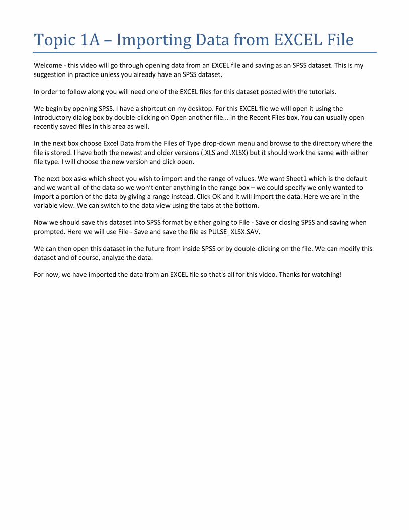
Welcome - this video will go through opening data from an EXCEL file and saving as an SPSS dataset. This is my suggestion in practice unless you already have an SPSS dataset.

In order to follow along you will need one of the EXCEL files for this dataset posted with the tutorials.

We begin by opening SPSS. I have a shortcut on my desktop. For this EXCEL file we will open it using the introductory dialog box by double-clicking on Open another file... in the Recent Files box. You can usually open recently saved files in this area as well.

In the next box choose Excel Data from the Files of Type drop-down menu and browse to the directory where the file is stored. I have both the newest and older versions (.XLS and .XLSX) but it should work the same with either file type. I will choose the new version and click open.

The next box asks which sheet you wish to import and the range of values. We want Sheet1 which is the default and we want all of the data so we won’t enter anything in the range box – we could specify we only wanted to import a portion of the data by giving a range instead. Click OK and it will import the data. Here we are in the variable view. We can switch to the data view using the tabs at the bottom.

Now we should save this dataset into SPSS format by either going to File - Save or closing SPSS and saving when prompted. Here we will use File - Save and save the file as PULSE_XLSX.SAV.

We can then open this dataset in the future from inside SPSS or by double-clicking on the file. We can modify this dataset and of course, analyze the data.

For now, we have imported the data from an EXCEL file so that's all for this video. Thanks for watching!

Topic 1B – Importing Data from CSV File

Welcome - this video will go through opening data from a comma separated or CSV file and saving as an SPSS dataset. This is NOT usually my suggestion in practice. I prefer to use EXCEL files if at all possible for the data I import into SPSS but it can import CSV files and many more file types.

In order to follow along you will need the CSV file for this dataset posted with the tutorials.

We begin by opening SPSS. I have a shortcut on my desktop. For this CSV file we will open it from inside SPSS so I am going to cancel the introductory dialog box. Inside SPSS I am going to go to File - Open - Data.

From here it looks the same as when we opened the EXCEL file. Now we choose TEXT from the Files of Type drop-down menu and browse to the directory where the file is stored. We choose the CSV file and click open.

Now we need to explain to SPSS exactly what type of format this text file uses. We do not match a predefined format so click next at the first screen.

The file is delimited which is already selected. However, our file does have the variable names in the header so we need to change this option to YES and then click next.

The first case of data begins on row 2 in our data which is the default. Each line represents a case - also true for our data. We want all of the cases. So click next here.

On this screen we select the delimiter which is comma for this data. Sometimes there might be quotes in the raw text file data and the qualifier will remove them if they exist and you specify the correct value in the qualifier area. We click next.

This screen allows you to check over the data and set all of the types. I usually wait and do this after I import the data but checking to make sure all of the data looks accurate at this point is a good idea and in our case it looks good so click next.

Finally - since you did all of this work to get here - SPSS asks if you would like to save this as a predefined format. This isn't necessary for our class so I am not going to go through this process.

For this course you can simply open the EXCEL file instead of the CSV to avoid this work, however, I wanted to go through this process as it does allow you to import a wide variety of data types and save those formats for later use if you will need them regularly in the future. In practice I see that this could be very useful.

Click finish when you are happy with all of your settings. You can go back and review them before you finish if you wish.

Now we save this dataset into SPSS format by either going to File - Save or closing SPSS and saving when prompted. Here we will close SPSS and go through the process.

In the first box we are warned that we are exiting SPSS and do we want to proceed. Answer Yes.

Then we are prompted to save the output. I will answer No.

Then we are prompted to save the dataset. I will answer Yes and save the dataset as PULSE_CSV.SAV.

We have imported the data from a CSV file so that's all for this video. Thanks for watching!

Topic 1C – Opening an SPSS Dataset

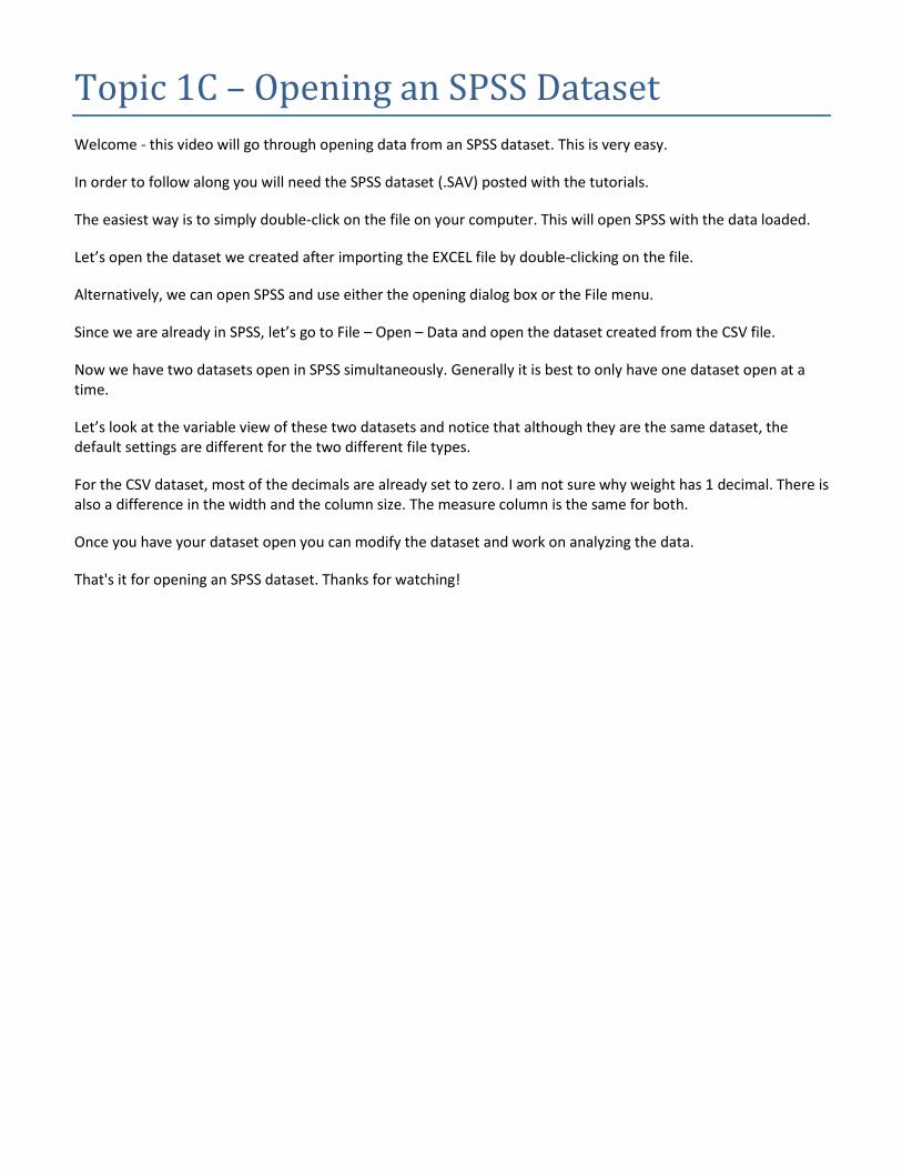
Welcome - this video will go through opening data from an SPSS dataset. This is very easy.

In order to follow along you will need the SPSS dataset (.SAV) posted with the tutorials.

The easiest way is to simply double-click on the file on your computer. This will open SPSS with the data loaded.

Let’s open the dataset we created after importing the EXCEL file by double-clicking on the file.

Alternatively, we can open SPSS and use either the opening dialog box or the File menu.

Since we are already in SPSS, let’s go to File – Open – Data and open the dataset created from the CSV file.

Now we have two datasets open in SPSS simultaneously. Generally it is best to only have one dataset open at a time.

Let’s look at the variable view of these two datasets and notice that although they are the same dataset, the default settings are different for the two different file types.

For the CSV dataset, most of the decimals are already set to zero. I am not sure why weight has 1 decimal. There is also a difference in the width and the column size. The measure column is the same for both.

Once you have your dataset open you can modify the dataset and work on analyzing the data.

That's it for opening an SPSS dataset. Thanks for watching!

Topic 1D – Importing Data from a SAS Dataset

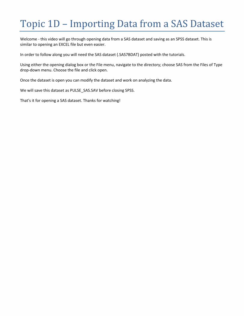
Welcome - this video will go through opening data from a SAS dataset and saving as an SPSS dataset. This is similar to opening an EXCEL file but even easier.

In order to follow along you will need the SAS dataset (.SAS7BDAT) posted with the tutorials.

Using either the opening dialog box or the File menu, navigate to the directory; choose SAS from the Files of Type drop-down menu. Choose the file and click open.

Once the dataset is open you can modify the dataset and work on analyzing the data.

We will save this dataset as PULSE_SAS.SAV before closing SPSS.

That's it for opening a SAS dataset. Thanks for watching!

Topic 2A – Basic Data Settings

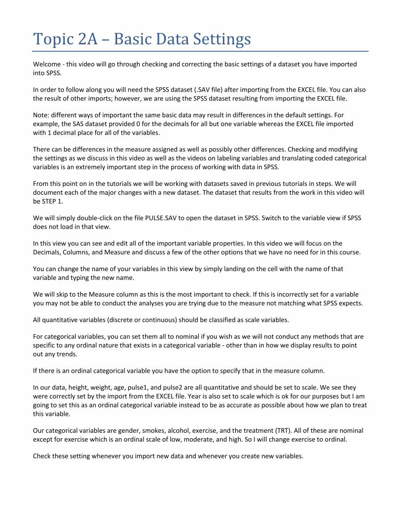
Welcome - this video will go through checking and correcting the basic settings of a dataset you have imported into SPSS.

In order to follow along you will need the SPSS dataset (.SAV file) after importing from the EXCEL file. You can also the result of other imports; however, we are using the SPSS dataset resulting from importing the EXCEL file.

Note: different ways of important the same basic data may result in differences in the default settings. For example, the SAS dataset provided 0 for the decimals for all but one variable whereas the EXCEL file imported with 1 decimal place for all of the variables.

There can be differences in the measure assigned as well as possibly other differences. Checking and modifying the settings as we discuss in this video as well as the videos on labeling variables and translating coded categorical variables is an extremely important step in the process of working with data in SPSS.

From this point on in the tutorials we will be working with datasets saved in previous tutorials in steps. We will document each of the major changes with a new dataset. The dataset that results from the work in this video will be STEP 1.

We will simply double-click on the file PULSE.SAV to open the dataset in SPSS. Switch to the variable view if SPSS does not load in that view.

In this view you can see and edit all of the important variable properties. In this video we will focus on the Decimals, Columns, and Measure and discuss a few of the other options that we have no need for in this course.

You can change the name of your variables in this view by simply landing on the cell with the name of that variable and typing the new name.

We will skip to the Measure column as this is the most important to check. If this is incorrectly set for a variable you may not be able to conduct the analyses you are trying due to the measure not matching what SPSS expects.

All quantitative variables (discrete or continuous) should be classified as scale variables.

For categorical variables, you can set them all to nominal if you wish as we will not conduct any methods that are specific to any ordinal nature that exists in a categorical variable - other than in how we display results to point out any trends.

If there is an ordinal categorical variable you have the option to specify that in the measure column.

In our data, height, weight, age, pulse1, and pulse2 are all quantitative and should be set to scale. We see they were correctly set by the import from the EXCEL file. Year is also set to scale which is ok for our purposes but I am going to set this as an ordinal categorical variable instead to be as accurate as possible about how we plan to treat this variable.

Our categorical variables are gender, smokes, alcohol, exercise, and the treatment (TRT). All of these are nominal except for exercise which is an ordinal scale of low, moderate, and high. So I will change exercise to ordinal.

Check these setting whenever you import new data and whenever you create new variables.

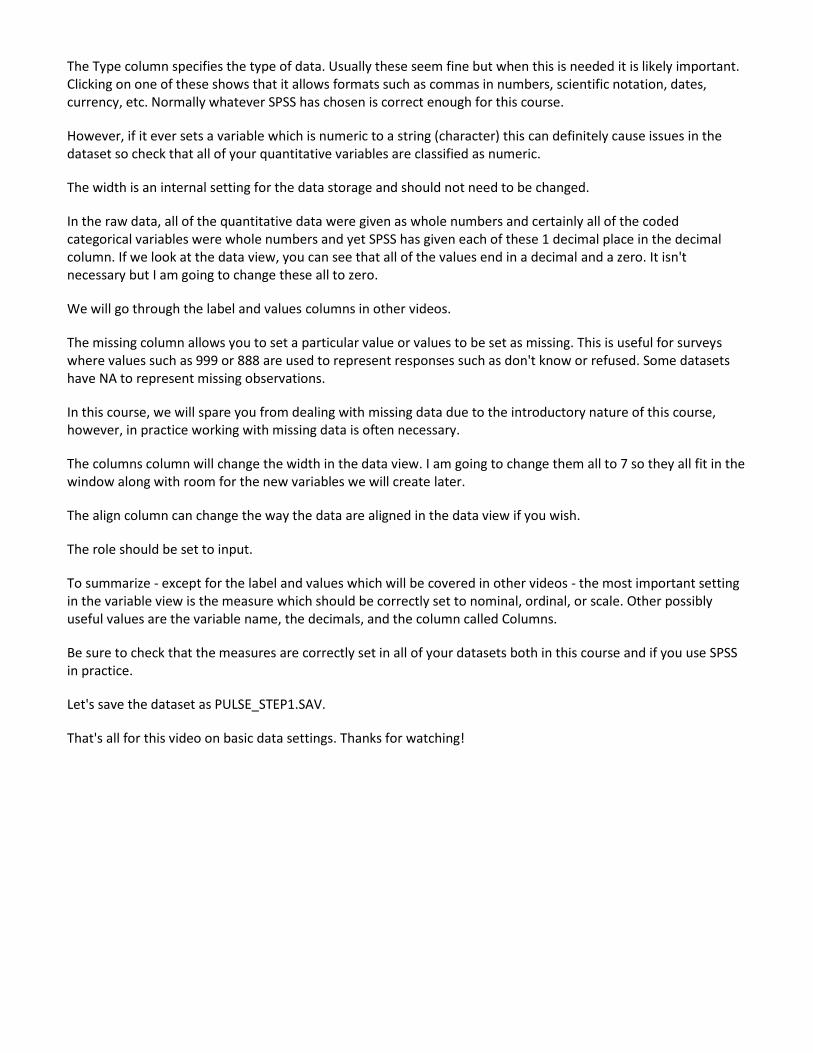
The Type column specifies the type of data. Usually these seem fine but when this is needed it is likely important. Clicking on one of these shows that it allows formats such as commas in numbers, scientific notation, dates, currency, etc. Normally whatever SPSS has chosen is correct enough for this course.

However, if it ever sets a variable which is numeric to a string (character) this can definitely cause issues in the dataset so check that all of your quantitative variables are classified as numeric.

The width is an internal setting for the data storage and should not need to be changed.

In the raw data, all of the quantitative data were given as whole numbers and certainly all of the coded categorical variables were whole numbers and yet SPSS has given each of these 1 decimal place in the decimal column. If we look at the data view, you can see that all of the values end in a decimal and a zero. It isn't necessary but I am going to change these all to zero.

We will go through the label and values columns in other videos.

The missing column allows you to set a particular value or values to be set as missing. This is useful for surveys where values such as 999 or 888 are used to represent responses such as don't know or refused. Some datasets have NA to represent missing observations.

In this course, we will spare you from dealing with missing data due to the introductory nature of this course, however, in practice working with missing data is often necessary.

The columns column will change the width in the data view. I am going to change them all to 7 so they all fit in the window along with room for the new variables we will create later.

The align column can change the way the data are aligned in the data view if you wish.

The role should be set to input.

To summarize - except for the label and values which will be covered in other videos - the most important setting in the variable view is the measure which should be correctly set to nominal, ordinal, or scale. Other possibly useful values are the variable name, the decimals, and the column called Columns.

Be sure to check that the measures are correctly set in all of your datasets both in this course and if you use SPSS in practice.

Let's save the dataset as PULSE_STEP1.SAV.

That's all for this video on basic data settings. Thanks for watching!

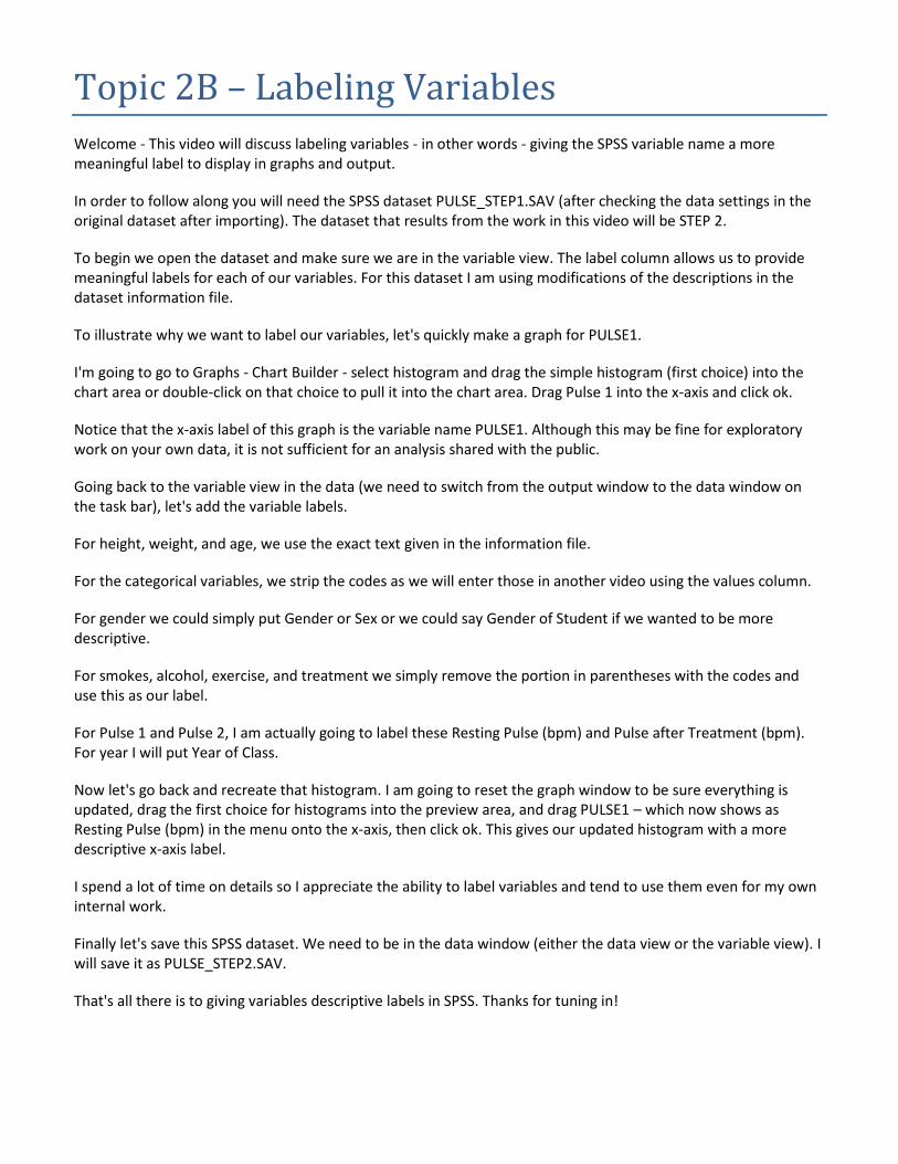
Topic 2B – Labeling Variables

Welcome - This video will discuss labeling variables - in other words - giving the SPSS variable name a more meaningful label to display in graphs and output.

In order to follow along you will need the SPSS dataset PULSE_STEP1.SAV (after checking the data settings in the original dataset after importing). The dataset that results from the work in this video will be STEP 2.

To begin we open the dataset and make sure we are in the variable view. The label column allows us to provide meaningful labels for each of our variables. For this dataset I am using modifications of the descriptions in the dataset information file.

To illustrate why we want to label our variables, let's quickly make a graph for PULSE1.

I'm going to go to Graphs - Chart Builder - select histogram and drag the simple histogram (first choice) into the chart area or double-click on that choice to pull it into the chart area. Drag Pulse 1 into the x-axis and click ok.

Notice that the x-axis label of this graph is the variable name PULSE1. Although this may be fine for exploratory work on your own data, it is not sufficient for an analysis shared with the public.

Going back to the variable view in the data (we need to switch from the output window to the data window on the task bar), let's add the variable labels.

For height, weight, and age, we use the exact text given in the information file.

For the categorical variables, we strip the codes as we will enter those in another video using the values column.

For gender we could simply put Gender or Sex or we could say Gender of Student if we wanted to be more descriptive.

For smokes, alcohol, exercise, and treatment we simply remove the portion in parentheses with the codes and use this as our label.

For Pulse 1 and Pulse 2, I am actually going to label these Resting Pulse (bpm) and Pulse after Treatment (bpm). For year I will put Year of Class.

Now let's go back and recreate that histogram. I am going to reset the graph window to be sure everything is updated, drag the first choice for histograms into the preview area, and drag PULSE1 – which now shows as Resting Pulse (bpm) in the menu onto the x-axis, then click ok. This gives our updated histogram with a more descriptive x-axis label.

I spend a lot of time on details so I appreciate the ability to label variables and tend to use them even for my own internal work.

Finally let's save this SPSS dataset. We need to be in the data window (either the data view or the variable view). I will save it as PULSE_STEP2.SAV.

That's all there is to giving variables descriptive labels in SPSS. Thanks for tuning in!

Topic 2C – Translating Categorical Variables

Welcome - This video will discuss the extremely important skill of translating the values of coded categorical variables.

In order to follow along you will need the SPSS dataset PULSE_STEP2.SAV (after labeling the original variables). The dataset that results from the work in this video will be STEP 3.

To illustrate why this is an important part of data preparation along with labeling and checking the measures of each variable. Let's look at a few pieces of output I created using the exercise variable.

In each of these results the values of exercise are given simply as 1, 2, and 3. Although it might be very easy for us to remember that 2 is moderate, it might be easy to switch high and low if we were not careful. The result of translating the coded categorical variables will place low, moderate, and high in the output instead of their codes.

Let's go back to the variable view. To create these translations we can use the Values column.

We start with gender. Clicking on the button with three dots in the values column for the variable gender we get this box. We place the code in the value box and the translation in the label box.

So we type 1 in the value box and Male in the label box and then we need to click add in order to save that translation. Then we type 2 in the value box and Female in the label box and click add. Then click OK.

We continue for the remaining variables, SMOKES and ALCOHOL are both 1 = Yes and 2 = No.

Don't forget to click add between each translation for each variable and don't click OK until you are done with the current variable.

For EXERCISE, we have 1 = High, 2 = Moderate, and 3 = Low.

For TRT, we have 1 = Ran and 2 = Sat.

Now here are those same results involving the variable exercise. We now see the translations for the codes instead of the codes.

Notice that the data view still shows the codes. We have not changed our raw data, only told SPSS to show us the values instead of the codes when it displays results involving these coded categorical variables.

Let's save this file as PULSE_STEP3.sav.

To summarize, in order to create translations we can use the values column in the variable view. We need to add each translation, clicking OK only after setting up the translations for all possible values for that particular variable.

Setting up these translations makes for easy reading of output which leads to an easier time of interpreting the results.

That's all for now. Thanks for watching!

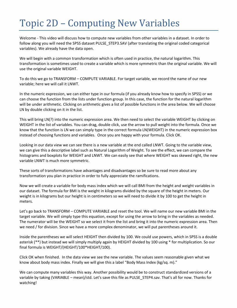
Topic 2D – Computing New Variables

Welcome - This video will discuss how to compute new variables from other variables in a dataset. In order to follow along you will need the SPSS dataset PULSE_STEP3.SAV (after translating the original coded categorical variables). We already have the data open.

We will begin with a common transformation which is often used in practice, the natural logarithm. This transformation is sometimes used to create a variable which is more symmetric than the original variable. We will use the original variable WEIGHT.

To do this we go to TRANSFORM – COMPUTE VARIABLE. For target variable, we record the name of our new variable; here we will call it LNWT.

In the numeric expression, we can either type in our formula (if you already know how to specify in SPSS) or we can choose the function from the lists under function group. In this case, the function for the natural logarithm will be under arithmetic. Clicking on arithmetic gives a list of possible functions in the area below. We will choose LN by double clicking on it in the list.

This will bring LN(?) into the numeric expression area. We then need to select the variable WEIGHT by clicking on WEIGHT in the list of variables. You can drag, double click, use the arrow to pull weight into the formula. Once we know that the function is LN we can simply type in the correct formula LN(WEIGHT) in the numeric expression box instead of choosing functions and variables. Once you are happy with your formula. Click OK.

Looking in our data view we can see there is a new variable at the end called LNWT. Going to the variable view, we can give this a descriptive label such as Natural Logarithm of Weight. To see the effect, we can compare the histograms and boxplots for WEIGHT and LNWT. We can easily see that where WEIGHT was skewed right, the new variable LNWT is much more symmetric.

These sorts of transformations have advantages and disadvantages so be sure to read more about any transformation you plan in practice in order to fully appreciate the ramifications.

Now we will create a variable for body mass index which we will call BMI from the height and weight variables in our dataset. The formula for BMI is the weight in kilograms divided by the square of the height in meters. Our weight is in kilograms but our height is in centimeters so we will need to divide it by 100 to get the height in meters.

Let’s go back to TRANSFORM – COMPUTE VARIABLE and reset the tool. We will name our new variable BMI in the target variable. We will simply type this equation, except for using the arrow to bring in the variables as needed. The numerator will be the WEIGHT so we select it from the list and bring it into the numeric expression area. Then we need / for division. Since we have a more complex denominator, we will put parentheses around it.

Inside the parentheses we will select HEIGHT then divided by 100. We could use powers, which in SPSS is a double asterisk (**) but instead we will simply multiply again by HEIGHT divided by 100 using * for multiplication. So our final formula is WEIGHT/(HEIGHT/100*HEIGHT/100).

Click OK when finished. In the data view we see the new variable. The values seem reasonable given what we know about body mass index. Finally we will give this a label “Body Mass Index (kg/sq. m).”

We can compute many variables this way. Another possibility would be to construct standardized versions of a variable by taking (VARIABLE – mean)/std. Let's save this file as PULSE_STEP4.sav. That's all for now. Thanks for watching!

Topic 2E – Categorize a Quantitative Variable

Welcome - This video will discuss how to categorize a quantitative variable. This is a skill often used in practice when there are commonly defined groups based upon a measured variable.

For example we might want to provide information about body mass index categorized into underweight, normal, overweight, or obese or classify individuals having high or low values for a particular variable such as high systolic or diastolic blood pressure. In addition there are often other reasons to categorize variables varying from the intended audience to the need to handle non-linear predictors in multiple regression analysis.

Here we will create a few different categorized versions. In particular we will categorize the body mass index variable (created in Topic 2D) into a binary version which looks at overweight (BMI ≥ 25) vs. not overweight (BMI < 25) and a multilevel version which categorizes into the standard categories. We will also categorize the variable WEIGHT in a similar fashion but the difference is that we won’t have any pre-defined grouping and will have to decide based upon the data.

In order to follow along you will need the SPSS dataset PULSE_STEP4.SAV (after computing new variables). We have the data open.

There are a few ways to do this in SPSS. In the TRANSFORM menu, we see some of these RECODE INTO SAME VARIABLES (this is not a good idea in general), RECODE INTO DIFFERENT VARIABLES, AUTOMATIC RECODE, VISUAL BINNING, and OPTIMAL BINNING.

RECODE INTO DIFFERENT VARIABLES gives a number of options and can be used for any variable type. This is particularly useful when recoding a categorical variable from text to a numeric code or collapsing/combining categories of a categorical variable. If you end up working with data in SPSS in practice, you may very well find this tool very useful.

For our current task, there is an easier tool. Go to TRANSFORM – VISUAL BINNING. We will start with body mass index since there are well-defined categories to be created. Pull BMI into the Variables to Bin list and click CONTINUE.

We start by creating a binary variable which looks at overweight (or worse) vs. less than overweight. We need to decide on a name for this variable in Binned Variable Name. I will call this variable BinaryBMI. By default it gives a label with (Binned) at the end of the original variable label. I will change this to “Binary Body Mass Index” instead.

The cutoff for overweight is a body mass index of 25. Click on the cell with the text “HIGH” and type 25 and enter. You can see the red line on the histogram indicating the cut-point created. This will create a value of 1 for all values less than or equal to 25 (because the default selection for the Upper Endpoints is “Included (<=)”) and a value of 2 for all values greater than 25. The HIGH represents the upper value of the last group is the highest observation.

We can add our translations here as well. Click on the label column for each value and type your translation. I will label the lower group “Normal or Underweight” and the upper “Overweight or Obese.” When you are happy with the settings click OK and then OK again in the pop-up box which should say that we will create 1 variable.

Looking at the data we can see we have a new variable BinaryBMI which is 1 or 2. In the variable view you can see and edit the label and values created in the tool.

If you make a mistake in the categorization you will need to delete the variable and go back through the process. You can delete a variable in the variable view by landing on the number in the column left of the variable name and hitting the delete key. I will undo that to get our variable back.

Now for the multilevel version. Go back to TRANSFORM – VISUAL BINNING and bring BMI into the Variables to Bin list. This should be the original quantitative variable, not the binary one we just created. Click CONTINUE.

We name this variable BMICAT and label it Body Mass Index Categories. The cutoffs needed are 18.5, 25, and 30. With values less than 18.5 being underweight, values between 18.5 and 25 being normal, then overweight, then obese.

Land on HIGH in the value column and type 18.5 and enter. Land on HIGH again and type 25 and enter. Then again for 30.

In the label column starting with that for 1 we give Underweight, Normal, Overweight, and finally Obese. When complete, click OK and OK again.

Now we will look at the variable WEIGHT. Go back to TRANSFORM – VISUAL BINNING and bring WEIGHT into the Variables to Bin list. Click CONTINUE.

We will start with the binary version which I will name BINWT and label Binary Weight. We can look at the histogram and decide on a cut point. I want to look at those with the highest weights and decided upon a value of 87 kg for my cut point. Land on HIGH and type 87 and enter. I will let SPSS create the translations for the values by clicking on Make Labels. Edit these or create your own if you wish.

Click OK and OK again.

Now for a multilevel version. Go back to TRANSFORM – VISUAL BINNING and bring WEIGHT into the Variables to Bin list. Click CONTINUE. I will name this variable WTCAT and label Weight Categories.

There are may ways to proceed from here depending on the application. You may know the values in which case, proceed as we did for BMI. You can use the histogram provided in the tool to help you decide on good values for cut points.

Here we will illustrate the automatic methods. Click on MAKE CUTPOINTS. Here you can make equal width intervals by providing at least two of the fields under that option. At the end you can choose to make cut points based upon the standard deviation rule choosing which values to use.

We will use the other option for Equal percentiles. You enter either the number of cut points (which is 1 less than the number of groups to be created) or the percentile in each group. We will create a 5-level variable where there will be approximately 20 percent in each group. For this situation we can enter 4 in the number of cut points or 20 in the width. Then click APPLY.

We will have SPSS create the translations by clicking on MAKE LABELS. Click OK and OK again to finish.

Let’s check our work by creating frequency distributions for the new variables with ANALYZE – DESCRIPTIVE STATISTICS – FREQUENCIES. And everything looks great.

We have successfully created a binary and a multilevel version for BMI and WEIGHT in our data. They are correctly labeled and translated and ready for further analysis.

Let's save this file as PULSE_STEP5.sav. That's all for now. Thanks for watching!

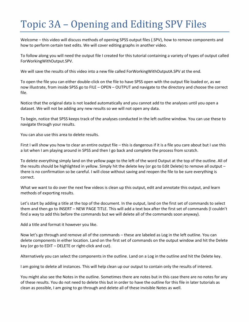
Topic 3A – Opening and Editing SPV Files

Welcome – this video will discuss methods of opening SPSS output files (.SPV), how to remove components and how to perform certain text edits. We will cover editing graphs in another video.

To follow along you will need the output file I created for this tutorial containing a variety of types of output called ForWorkingWithOutput.SPV.

We will save the results of this video into a new file called ForWorkingWithOutputA.SPV at the end.

To open the file you can either double-click on the file to have SPSS open with the output file loaded or, as we now illustrate, from inside SPSS go to FILE – OPEN – OUTPUT and navigate to the directory and choose the correct file.

Notice that the original data is not loaded automatically and you cannot add to the analyses until you open a dataset. We will not be adding any new results so we will not open any data.

To begin, notice that SPSS keeps track of the analyses conducted in the left outline window. You can use these to navigate through your results.

You can also use this area to delete results.

First I will show you how to clear an entire output file – this is dangerous if it is a file you care about but I use this a lot when I am playing around in SPSS and then I go back and complete the process from scratch.

To delete everything simply land on the yellow page to the left of the word Output at the top of the outline. All of the results should be highlighted in yellow. Simply hit the delete key (or go to Edit Delete) to remove all output – there is no confirmation so be careful. I will close without saving and reopen the file to be sure everything is correct.

What we want to do over the next few videos is clean up this output, edit and annotate this output, and learn methods of exporting results.

Let’s start by adding a title at the top of the document. In the output, land on the first set of commands to select them and then go to INSERT – NEW PAGE TITLE. This will add a text box after the first set of commands (I couldn’t find a way to add this before the commands but we will delete all of the commands soon anyway).

Add a title and format it however you like.

Now let’s go through and remove all of the commands – these are labeled as Log in the left outline. You can delete components in either location. Land on the first set of commands on the output window and hit the Delete key (or go to EDIT – DELETE or right-click and cut).

Alternatively you can select the components in the outline. Land on a Log in the outline and hit the Delete key.

I am going to delete all instances. This will help clean up our output to contain only the results of interest.

You might also see the Notes in the outline. Sometimes there are notes but in this case there are no notes for any of these results. You do not need to delete this but in order to have the outline for this file in later tutorials as clean as possible, I am going to go through and delete all of these invisible Notes as well.

Now let’s look at a print preview of the file. Be certain you are not selecting any particular output in the output view then go to FILE – PRINT PREVIEW. Looking through, notice that the page title caries through the entire document. Notice also that the wide tables are broken into as many sub-tables as needed. We will solve some of this by removing output.

Ok, back to a few other edits. Looking through the output, there are a few tables which might not be useful.

For frequencies – this first table with the statistics – let’s delete this and again before the pie chart. Let’s delete the title of frequencies before the pie chart.

Under explore, we delete the title frequency of exercise and the case processing summary and at the end the tests of Normality. Let’s remove all of the stem-and-leaf plots and the titles above them.

Above the histogram, delete the titles and statistics table. Under Crosstabs, delete the case processing summary.

The remaining titles can be edited or deleted. I will change them to indicate solutions to questions for example. Double click on the first title and change it to say Question 1.

I will change explore to read Question 2.

Land on the side-by-side boxplots and go to INSERT – NEW TITLE – this will insert a new title after the graph. We type Question 3.

We change the remaining titles to Question 4, 5, and 6 respectively.

Go back and preview the file – make sure you are on the file and not selecting a certain portion of output.

You can see the results are cleaner but we still have some work to make it export nicely from SPSS.

That is all we will do in this tutorial. We save the results as ForWorkingWithOutputA.SPV. Thanks for watching!

Topic 3B – Editing Graphs in SPSS Output

Welcome – this video will go through some optional skills in editing graphs in SPSS. We can resize, recolor, and make other adjustments.

In order to follow along you will need the output file ForWorkingWithOutputA.SPV after our first round of cleaning up the original SPSS output for these Topic 3 tutorials.

At this stage we have removed all unwanted components including all Logs and Notes, any unneeded output tables such as case processing summaries, and unwanted titles.

Now we will work on the graphs. Firstly, most of the graphs are too large for nice results in either SPSS or copied into Word. We can resize them in SPSS simply by landing on the graph and dragging the corner or edge boxes appropriately.

I will make all of the graphs a little smaller and adjust as needed later. I like resizing in Word a little better since you can redo particular height or width settings based upon your image and page sizes.

All SPSS output components, including graphs, can be edited by double-clicking on them. But for graphs, there are usually some useful options for editing components such as titles, labels, axes, colors, and fonts which might be needed in practice.

Let’s start with the bar chart. Double-click on the chart to open the editor window. Double-clicking on components will allow you to change them. I will double-click on the background to and change the background color to white. Click apply and close. Then I will double click on any one of the bars and change the color to green, click apply, and close. Close the window to complete the editing.

Now the pie chart. Double-click on the chart to open the editor window. You can maximize if you wish. If we double click on the chart it will select the pie itself – but we would likely want to change the colors of slices so click again once on any slice. You should notice it outlines that component and highlights it in the legend. Now double-click to change the options for that slice.

You can choose the fill and border colors and a fill pattern. The weight applies to the border of that slice. Click apply and close. You can edit any of the text in the chart. You could change the background color – but I like the white background as is.

You can add your own titles, footnotes, and text boxes. You can decide whether to display the legend. Be sure to apply all changes and then close the editor when you are finished.

Now let’s edit the boxplots. Double-click on the graph to open the editor window. You can remove the labels on the outliers by clicking on them to select them and hitting the Delete key. You can change colors. I usually like to remove the grey background. Double-click on the area change the color to white and close. For text and graph element colors try double-clicking on the component and looking for the color settings.

To change an axis scale, double-click on the axis (here we will use the y-axis) and go to the scale tab. Here you can change the way the axes display. Be careful not to cut off any data. SPSS gives you the min and max in your data to help you avoid this. Let’s change the increment to 10 instead of 25 and click apply and then close.

You could add a horizontal reference line to this chart to compare to some norm, say a pulse of 70 beats per minute. Click on the Add reference line to Y-axis either in the OPTIONS menu or in the toolbar and enter 70 in the

position box. You can have it choose the mean or median automatically as well. Click apply before moving to any other tabs. You can format the line how you desire. Apply all changes and then close the editor.

For the histogram, we could do similar edits. We could delete the text box with the summary measures, we could change colors, edit text, add text, add annotations, add horizontal or vertical reference lines. The possibilities are endless and none of them are important for the concepts in this course! Here’s what I came up with.

For the scatterplot, I do want to show you how to change the data labels on these grouped scatterplots because the default color choice in SPSS is a very poor one! Double-click on the plot to open the editor.

These methods are similar for a regular scatterplot but for a grouped scatterplot we want to set up the markers and colors for each group to be clearly different from each other which requires selecting the appropriate points.

The easiest way is to use the legend. Click on the symbol in the legend for Males and this will select all of the males. Then double-click on any selected point to open the editor for the points for males. I am going to choose blue triangles for the males and increase the size to 8. Click apply and then close.

Select Females and double-click, I will leave the circles but change them to purple, click apply and close. In both cases I made the fill and border the same color but you have many options to choose from. The goal is to make it easy to distinguish even for color-blind individuals or if the graph is duplicated in black and white.

That is plenty about editing graphs. We don’t ask you to modify SPSS graphs in any way in this course but in practice you will often need or want to change the look of your graphs from the SPSS default.

Let’s save the result as ForWorkingWithOutputB.SPV. Thanks for watching!

Topic 3C – Editing Tables and Page Breaks

Welcome – this video will discuss how to edit some of the tables in SPSS output and how to insert page breaks into our edited output.

To follow along you will need the SPSS output file ForWorkingWithOutputB.SPV after our second round of edits involving the graphs.

This is not normally something I do but for those of you who might be interested, I will show you what you can do in SPSS to edit the resulting output tables.

Let’s start at the top with the year of class. Double-click on the table to edit. I usually close the window with the pivot trays. The formatting toolbar might be useful. We may want to delete the columns of valid percent and cumulative percent for this table. Select the values in those columns and hit the delete key.

Click outside of the table to save the results. Now let’s double-click on the result of explore in the descriptives table. We will remove the 5% trimmed mean, variance, skewness, and kurtosis. We need to select the three columns for those rows and hit the delete key – notice that the titles disappear from other groups but not the values and cells. Close the window when you are done.

Now we double-click on the percentiles table. First, I will copy the text that is the same between these two rows. Then, I will select the bottom row starting from the far lower right corner all the way back through the label for Tukey’s hinges and delete all of those results. Then reselect the area where the labels I copied were located and paste them back into place.

We only need the quartiles so I can delete all of the other values. I will leave the median. Close the window when finished.

I don’t have any edits for the two-way tabled labeled as Question 4 or the t-test table in Question 5. So that’s all of the table edits I will make in this file. Do not feel you need to edit output in this way for this course but you are welcome to do so as long as your results contain the requested information.

Now let’s look at the print preview and begin deciding where we would like our page breaks. To place a page break, select an item which will start a new page and go to INSERT – PAGE BREAK. To clear the page break, select the item and go to INSERT – CLEAR PAGE BREAK.

We can also insert text between output for spacing but for these we need to land on the item BEFORE where we wish the text to be placed. Then click on INSERT – NEW TEXT.

Here is the final print preview at this stage. Notice the two-way table using crosstabs and the t-test results still have tables that wrap in order to display all of the results.

That’s all for this video on some final options for editing SPSS output including editing tables and adding page breaks. Let’s save the output as ForWorkingWithOutputC.SPV. Thanks for watching!

Topic 3D – Exporting and Copying Output

Welcome – this video will cover using SPSS to export results into PDF, RTF, and copying output into Word. These skills are useful for preparing solutions in this course and in practice for sharing with colleagues. To follow along you will need the SPSS output file ForWorkingWithOutputC.SPV after our final round of edits involving the tables and page breaks.

You do not need to edit your output in this course but you will need to present your results in documents for assignment submissions. We will begin with exporting the results using SPSS’s export capabilities.

We can export all results by going to File – Export – and making sure that All is selected in the objects to export area at the top. The default seems to be a WordRTF (.doc) format.

You need to carefully select the location. This does not work like most save features in that it automatically saves your last location and file name – which might be useful but can also be a problem. Choose a location and a file name. We will save this file as ForWorkingWithOutputD.doc.

The options give us some choices regarding how the document is created. In particular, you can choose how to handle wide tables – split by wrapping, shrink to fit, or let it exceed the margin. We will set this to shrink for the word document and click continue and OK to export the file.

Another way to export all results is to right-click on the output in the outline view and choose export. This time choose pdf from the type menu and decide the location and file name, we will save this file as ForWorkingWithOutputD.pdf. Interestingly the PDF option does not allow shrinking the wide tables but does allow for exporting bookmarks. Click ok to save the pdf file.

There are other file types but those are the two that will likely be useful to you in this course and elsewhere.

Let’s look quickly at those files. Here is the Word document – some of the pages are not aligned the same as in SPSS but you can fully edit this word document and save it in a new Word format or save it as a pdf.

Here is the result of shrinking the table for the independent samples test, we may not have discussed this output yet but you can clearly see the text is much smaller. We can edit this table in Word by increasing the font size and resizing columns as needed.

Here is the PDF file which looks exactly like our print preview in SPSS but cannot be easily edited.

Those are some options for exporting results directly from SPSS but I normally copy the needed results into a Word document directly to create my summaries. For most results you can simply copy using Edit – Copy or CTRL – C in SPSS and then paste into your Word document.

For copying tables into word, there are a few options, if you want the format to look like it did in SPSS then choose keep source formatting. If you want it to have the format for your current word document, choose merge formatting, and there is also plain text. Here is what each of these results would look like for my document

Graphs copy easily and there is no difference between the two paste options.

Wide tables cause students some frustration and I will take anything that contains the correct information no matter how unpleasant it may look.

My two favorite options are to copy and paste in the default way and then edit the table in Word. To do this simply copy the table and paste it into Word. I select the entire table and right-click and choose auto-fit to contents. Possibly I will resize the font a little to make the table as nice as possible. You can format from here further.

The other option is to copy and paste as an image. To do this, select the item in SPSS and right-click and choose Copy Special. Select image from the list (you can choose your default copy special by checking the box) and click OK. Go to your Word document and paste the image and resize as needed to fit the page.

Let’s save this Word document we created from copying and pasting as ForWorkingWithOutputD.docx.

That’s it for working with SPSS output although I am certain there is a lot more that SPSS can do. Thanks for watching!

Topic 4A – Frequency Distributions

Welcome - this video covers creating frequency distributions for categorical variables.

In order to follow along you will need the SPSS dataset PULSE_STEP3.SAV (after translating the original coded categorical variables).

Let's open the data.

To create frequency distributions, we go to ANALYZE - DESCRIPTIVE STATISTICS - FREQUENCIES.

In the dialog box, there are at least two ways to pull variables into the analysis variables area. You can click on a variable and then the arrow or you can drag the variable into the list. If you want to select multiple variables, hold down the CTRL key while you click to select multiple variables.

We will analyze all of our categorical variables at one time so I select GENDER, SMOKES, ALCOHOL, EXERCISE, and TRT and drag them into the variable(s) list.

We could just click OK to get the default tables but generally we will discuss the options available, some of which will be important to use regularly.

For using FREQUENCIES with categorical variables under the STATISTICS options we don't want any of this for categorical variables.

Sometimes, with ranking variables you might want the mean and standard deviation of the response. We will see later that FREQUENCIES can be used for simple summaries of one quantitative variable which is when these values are useful.

We will cancel the STATISTICS options.

Under CHARTS, for a categorical variable you can choose None, Bar Charts, or Pie Charts - the histogram option would be for a quantitative variable.

Unfortunately you can only get one graph at a time. We will select Bar Charts this time and then come back and ask for the pie charts. After selecting Bar Charts, you can decide if you want the chart to display frequencies or percentages. I am going to select percentage and click on continue.

The FORMAT options are usually fine with the default, however you can choose how to order the possible values - ascending values (1, 2, 3, 4), descending values (4, 3, 2, 1), ascending counts which would order categories by how common they were from least to most common, and descending counts where categories are ordered from most common to least common.

I will also point out that for quantitative variables, the box for Suppress tables with many categories can be useful. However we can also control this in the main box.

We will leave this as it is, click on continue or cancel.

The STYLE options are new to SPSS 22. I don't know anything about this but I assume it allows you to create certain standard formatting styles which can be implemented in this option. We won't use this option in this course.

We also will not learn about the bootstrap options which you will see in many of the analyses we conduct. This is a higher level topic than our course but you are welcome to read the SPSS documentation or research the topic of bootstrapping on your own.

So to review, we have not changed anything in STATISTICS, FORMAT, STYLE, or BOOTSTRAP. We have asked for bar charts in the CHARTS options.

Before we click OK, note that there is the checkbox for whether or not you want to display the frequency tables. Since that is the purpose of this tutorial, we will leave this checked but if you only want the graphs or if you analyze a quantitative variable using FREQUENCIES then unchecking this box is a good idea. We will illustrate this when we create the pie charts and again when we talk about quantitative variables.

Notice we expect 6 variables to be analyzed. Click OK when ready.

First we get a summary of the sample sizes for each variable. In this dataset there is no missing data so we see 107 as the valid N and 0 missing for each variable.

Then we get the 6 frequency tables. Each table gives the possible values, the frequency of each value in our dataset, the percent and the valid percent - if there were missing observations, the percent would include the missing values in the total whereas the valid percent would divide only by the valid N.

Finally we also get the cumulative percent which might be useful for an ordinal categorical variable. For example, in exercise, the cumulative percentage for moderate of 66.4 means that 66.4% were moderate or high (2 or 1 on the original scale).

It helps not having to add the percentages ourselves when we want the percentage at or below a particular level in an ordinal variable. We can find also find the percentage above a particular level by subtracting the cumulative percentage from 100.

Generally we want to know the sample size and the percentage in each category. The frequencies are less useful than percentages as a summary measure.

After the frequency tables, we get the bar charts we requested. We will cover editing charts and output in other tutorials.

Let's go back into ANALYZE - DESCRIPTIVE STATISTICS - FREQUENCIES and ask for the pie charts instead. Notice that our settings are the same. You can always reset any SPSS tool using the Reset button. Here we want the same variables so we will simply go to Charts and select pie charts instead of bar charts.

Now we could get the frequency tables again but we already have them so this time I will uncheck the box for Display frequency tables so that we only get the graphs. Click OK.

Now we have the pie charts for these variables.

Technically we have covered creating frequency tables, bar charts, and pie charts, however; we will also illustrate how to create bar charts and pie charts individually using the GRAPHS - CHART BUILDER tool in other videos. There are also other videos covering how to edit, export, and copy results.

We haven't made any changes to the dataset so we don't need to save the data but we have created output which we will save into an SPV file. We need to be in our output window and go to File - Save. I will save this file as OneCatVarFrequencies.SPV

That's all for creating frequency distributions for categorical variables. Thanks for watching!

Topic 4B – Creating Bar Charts and Pie Charts

Welcome - This video will illustrate how to use the chart builder to create a bar chart and a pie chart.

In order to follow along you will need the SPSS dataset PULSE_STEP3.SAV (after translating the original coded categorical variables). Let's open the data.

To create a bar chart we go to GRAPHS - CHART BUILDER. The box that pops up is warning you to make sure all of your variable properties are correctly set. For us that means having set the measures, labels, and translations for the data, which we have done. If you prefer not to see this box in the future you can check the box for don't show this dialog again.

Click OK. This brings up the chart builder window. To select a chart choose the correct type from the text list on the bottom left and either double click or drag the chosen graph type from the pictures on the bottom right into the preview area. .

Bar chart is the default. We want the first, simple bar chart. You do need to understand the graphs you want. In this case there is both an x-axis and a y-axis but we only need to drag the categorical variable onto the x-axis.

We do not want to drag any variable onto the y-axis as this will be the count or percent within each category. Just because SPSS gives you the option to put something on the graph area doesn't mean you should.

Let's drag exercise onto the x-axis. Notice that now it does give us the Count as the y-axis now that we have selected a categorical variable to analyze. The preview does not reflect your data the actual graph will look different. In the element properties, we can choose count for the y-axis or percent. The other values don't make sense for our current situation but this graph builder does allow for creating more complex displays.

I am going to set the statistic to percentage. Any changes made in the element properties will not be made on the graph until you click the apply button. If you forget to click the apply button there will be no changes applied.

Click apply to change the statistic to percentage. Then click OK. This gives a bar chart for Exercise. Notice it was easier to use the FREQUENCIES and simply ask for the bar charts as this gave all of the bar charts with one tool. We would need to repeat the chart builder process for each variable individually which is time consuming.

Now let's create a pie chart for exercise. We go back go GRAPHS - CHART BUILDER, click OK in the box if you haven't disabled it.

Notice that in the same SPSS session, the chart builder (and other tools) will keep our most recent settings. This is useful if you made an error and you can quickly repeat the process changing only what is needed. All tools can be reset with the reset button.

Here we want a pie chart for Exercise so let's select Pie/Polar from the list and select the pie chart - either double click or drag the picture into the graph preview area.

It did correctly keep exercise as our analysis variable. Again I will change count to percentage and click apply. Then click ok to see our pie chart. We will talk about editing and copying output in other videos.

Let's save this output as OneCatVarGraphs.SPV.

That's all for this video on creating bar charts and pie charts for one categorical variable using the chart builder tool. Thanks for watching!

Topic 5A – Numeric Measures using EXPLORE

Welcome – this tutorial will cover calculating numeric measures for one quantitative variable using EXPLORE.

In order to follow along you will need the SPSS dataset PULSE_STEP3.SAV (after translating the original coded categorical variables). We begin by opening the dataset.

Although in a later video we will discuss two other ways to calculate numeric summaries for one quantitative variable, EXPLORE will be the only one that is useful for exploring the relationship between a quantitative variable and a categorical variable so it is preferred and covered first.

To conduct this analysis we go to ANALYZE – DESCRIPTIVE STATISTICS – EXPLORE. We can explore all of our quantitative variables at once using this tool. We select our quantitative variables height, weight, age, pulse1, and pulse2 – drag those into the dependent list.

You can see that we will have the option to put in a factor variable but for now we don’t want to break up the variable, we want to see the summary for the overall results for all subjects for each of these variables.

Under statistics, the descriptives is checked by default along with the percentage used for the confidence interval for the population mean based upon our sample.

We definitely want the descriptives so leave this box checked. Check the percentiles box I you need the quartiles as they are not provided in the default descriptives. We will check that box and click on continue.

Under the plots options we can select a histogram and normality plots (QQ-plots). If you prefer not to see the stem-and-leaf displays you can uncheck the box .

The stem-and-leaf display can be useful since we can see the actual data values, although SPSS sometimes cuts off the upper or lower extremes and just tells you how many there were above or below the specified value.

The boxplots setting relates to how it organizes boxplots when we are looking at relationships between a quantitative variable and a categorical variable. I almost always leave this setting as it is in all situations.

I am going to check the histogram box and the normality plots box and click on continue.

You have the choice whether to create the numeric results (statistics) or the plots or both. We will leave this set to both.

To review, we added our quantitative variables to the dependent list. We added percentiles in the statistics, we selected the histogram and normality plots in the plots and made no changes to the options or bootstrap.

Click OK to see the results. We see the case processing summary which gives the valid (non-missing) N for each variable, the count for any missing observations (we have none) and the overall N for each variable which would include the missing observations. This lets you see what percent of your original sample size have missing observations for any given variable.

Then we see a large descriptives table containing the same numeric summary measures for each variable. We are interested in the mean, later we will want the confidence interval for the mean but we will already know how to obtain it. We want the median, standard deviation, minimum, maximum, range, and IQR.

We also see the skewness and kurtosis which are measures of the shape of the distribution. You can search online if you are interested in learning more about them. They can be useful in determining how skewed a distribution is

and how close to a normal distribution you have based upon your sample. Currently, we don’t cover these measures in this course.

The 5% Trimmed mean, which we also do not cover, is the mean after removing the upper 5% and lower 5%. This measure is more resistant to outliers, more robust and thus should be a better measure of the center for distributions with outliers or slight skewness. Extreme skewness would still impact the 5% trimmed mean.

We also see the variance which we have discussed in the course materials but usually we prefer the standard deviation to the variance.

For a few values – the mean, skewness, and kurtosis, we also get a value called the standard error. This is a measure of the variability of our statistic in repeated sampling – if we were to do this again and again, the standard error represents the standard deviation of all of the sample means we would collect.

In this case for height, which has a standard error of about 1 for the sample mean of 173.3, if heights are approximately normally distributed the standard deviation rule would say that we would expect 95% of the sample means to be between 171.3 and 175.3 if we were to repeat this study a large number of times.

We will talk a lot more about this later but I wanted to introduce the idea since we are given this value in the table and you might immediately wonder what it represents.

After the descriptives table we have the percentiles. We mention in the course materials that software packages may differ in their answers for Q1 and Q3 and indeed here we see some differences in the two methods used by SPSS.

For the weighted average approach we also get the 5th, 95th, 10th, and 90th percentiles in addition to the quartiles. For Tukey’s hinges we only get the quartiles. I will take either in solutions to assignments, however, our solutions will use the first set – the weighted average.

Then we get tests for normality. We might discuss these later in the semester after we learn hypothesis testing but these are not an official part of our course content. They allow hypothesis test based decisions for whether normality is reasonable or not but there are issues with these tests and I don’t usually rely on them even though I may look at them in addition to the graphical and numeric methods we have discussed.

Now we see the graphs. For each variable we get a histogram with the mean, standard deviation, and sample size given on the upper right outside of the plot. There is no option in the EXPLORE tool for putting the percentage instead of the frequency on the y-axis but we will see this can be done in the chart builder.

Then we get a stem-and-leaf display. You can see that it doesn’t show the lowest value, only that there is 1 extreme below 140.

Then we get the QQ-plot with a reference line. We also see a detrended QQ-plot. This looks at the difference between the points and the reference line and graphs those differences allowing us to more easily spot patterns and outliers which are masked by the y-axis scale of the QQ-plot itself. I will not ask for these in solutions to assignments but you can have them if you wish.

Finally we have the boxplot. Notice that it does mark the outliers with their observation number.

Let's save this output as OneQVarExplore.SPV.

That’s all for this video on calculating numeric measures for one quantitative variable using EXPLORE. This is very useful, with one tool we have found all of the numeric measures we need as well as all of the graphs for all of our quantitative variables. I think that is pretty exciting! That’s it for now. Thanks for tuning in!

Topic 5B – Creating Histograms and Boxplots

Welcome – this video covers creating histograms and boxplots using the chart builder. This will be similar to creating a bar chart.

In order to follow along you will need the SPSS dataset PULSE_STEP3.SAV (after translating the original coded categorical variables). Let’s open the data.

To begin we go to GRAPHS – CHART BUILDER – click OK in the warning box if you haven’t disabled it.

Choose histogram from the lower left menu and drag the first choice into the preview area.

Choose a quantitative variable and drag it onto the x-axis. I am going to choose height. We can have it display percentages by choosing histogram percent from the statistic drop-down menu in the element properties and click apply. Then click OK.

Except for the y-axis, this graph is the same as we obtained from checking this histogram box in EXPLORE.

To create the boxplot return to GRAPHS – CHART BUILDER and select boxplot from the lower left menu. This time we want the LAST option, the single boxplot. Boxplots are most commonly used to compare groups so likely that is the reason the first choice for boxplots is for comparing groups.

Drag the variable onto the y-axis this time, we will use height again and notice it is already set. Remember you can reset any tool using the reset button. Click OK. There are no settings to change for boxplots.

The boxplot and histogram for height both show a very symmetric distribution with one outlier. If you look at the numeric summaries you will see that the mean and median are very close together relative to the variation (as measured by the standard deviation or IQR).

You can also see that by default SPSS provides the observation number for any outliers so that you can easily find them in the dataset and check for and fix any errors, remove observations found to be errors that cannot be repaired, etc.

Let's save this output as OneQVarHistBox.SPV.

That’s it for creating histograms and boxplots using the chart builder. We will look at editing results in another video. Thanks for watching!

Topic 5C – Creating QQ-Plots and PP-Plots

Welcome – this video will illustrate creating QQ-Plots and PP-Plots.

In order to follow along you will need the SPSS dataset PULSE_STEP3.SAV (after translating the original coded categorical variables). Let’s open the data.

In our course QQ-plots are generally preferred but PP-plots are designed to do the same thing – provide a visual comparison to a theoretical normal distribution to see how closely our data are to being precisely normally distributed.

Interestingly these are not available in the chart builder but under ANALYZE – DESCRIPTIVE STATISTICS.

We start by choosing QQ-plots since they are our preference. Unlike the chart builder – more like EXPLORE, we can analyze multiple variables simultaneously. We will drag in all five of our quantitative variables. Leave the settings at their default values and click OK.

These graphs are the same as those obtained by using EXPLORE. The only differences are in the numeric measures we obtain in the two procedures none of which are of particular interest.

Now we go back to ANALYZE – DESCRIPTIVE STATISTICS and choose PP-plots. Again drag in all five of our quantitative variables. Leave the setting at their default values and click OK.

These graphs are displaying the same information but the scale is based upon the probabilities instead of the values of the original variable which considerably alters the scale. At the low end of the distribution a small difference in probabilities can be relatively far away in terms of variable values whereas closer to the center a small difference in probabilities will result in a much shorter distance between variable values.

Again, we prefer QQ-plots to PP-plots but the both show the same trend, just on a different scale.

For both QQ-plots and PP-plots, we get detrended results which are always optional for any assignments in this course.

Let's save this output as OneQVarQQplot.SPV.

That’s all for creating QQ-plots and PP-plots. Thanks for watching!

Topic 5D – Numeric Measures: Other Methods

Welcome – this video discusses two other methods for obtaining numeric measures for one quantitative variable.

In order to follow along you will need the SPSS dataset PULSE_STEP3.SAV (after translating the original coded categorical variables).

The methods used in this video are great for summarizing one quantitative variable, however, they do not allow for investigation of the relationship between a quantitative variable and a categorical variable and thus are very limited in their overall usefulness in practice. You can split a dataset by a categorical variable and then analyze each dataset but this is somewhat clumsy and not needed given EXPLORE will give everything we need.

To begin we go to ANALYZE – DESCRIPTIVE STATISTICS – DESCRIPTIVES. We can analyze all five of our quantitative variables simultaneously so let’s drag them into the variables list. Notice that there is only room for one set of variables – no way to break this down by any other variable.

In options we can choose which measures we see. You might want to add the range but generally the default settings are fine. Notice there is no choice for the median, Q1, or Q3. I find this to be a reason NOT to use this tool. I will leave the default setting and click on continue.

The style is something new to version 22 which we won’t change. We also don’t need the bootstrap. There is a check-box for save standardized values as variables. This could be useful. We will illustrate how to manually create standardized variables in another video but let’s check this box and see what happens.

Click OK to see our results.

One nice thing about this method is that the table is much easier to read than that obtained from EXPLORE. If you just need this simple summary of your quantitative variables, it is a great tool. However, in our course we normally want the median and quartiles which make this method less useful.

If we go to our dataset we see that we now have five new variables named as the original variables with a Z in front. These give the z-scores for each observation for each variable. So for example the 2nd observation has a PULSE2 measurement of 150 which corresponds to a z-score of 1.7. This person has a 2nd pulse rate which is 1.7 standard deviations about the average PULSE2 value.

Now let’s look at the last method. Go to ANALYZE – DESCRIPTIVE STATISTICS – FREQUENCIES. We used this same tool for constructing frequency distributions for categorical variables. Now we will use it to calculate summary measures for quantitative variables.

Reset this tool if you have already used it in this SPSS session. Drag in the five quantitative variables and go to statistics. I will select quartiles, mean, median, std. deviation, range, minimum, and maximum and click on continue.

For charts, we can select histograms and check the box for normal curve on histogram. And click on continue.

For format, we discussed earlier that the order by might be useful for categorical variables and maybe if you prefer to see things descending it might be useful for quantitative variables but we will leave this as default.

The multiple variables option does allow us to choose how to organize the output – as a comparison of variables or organize output by variables. We will leave the defaults here as well and click on continue.

We won’t make any changes in the style or bootstrap.

Before we finish, notice that we have this check-box for whether we want frequency tables. I am going to leave it checked for now to show you why you do not want to leave this checked when using this tool to analyze quantitative variables.

Click OK to see the results.

The first table gives the summary statistics. The histograms are at the end. In between since we did not uncheck the box for displaying frequency tables, we get tables containing each possible value and how often they occur. This is usually not helpful for quantitative variables except possibly for data checking.

Looking through these tables, all of the variables except for age have long and difficult to read frequency tables which would not be of interest. Please don’t provide these in documents submitted in this course as they are not needed and take up a too much space.

I am going to remove the output we just created. Now I can go back in and uncheck that box and click OK.

Now we have only the results of interest. This does provide all of the measure we are interested in finding in a very nicely organized fashion. However, since it doesn’t allow us to break up a variable by a categorical variable, it is less useful in general, it is useful only for one quantitative variable at time.

The histograms are nice because they add the normal overlay so you may decide to use this for histograms instead of EXPLORE or the chart builder.

We will discuss the output in entirely separate videos but note here that PULSE2 is clearly two groups of individuals. The lower group represents individuals who stayed seated and the higher group represents the group that ran. It will be interesting to start breaking variables down by this treatment variable.

To review FREQUENCIES and DESCRIPTIVES can also be used to obtain some numeric summary measures for quantitative variables. They allow for analyzing multiple variables simultaneously and the frequencies option creates very nice histograms with normal curve overlays.

The problem with these two tools is that they can only look at an entire variable. In order to break down the results by a categorical variable, we need to do this manually. We will cover some of these methods in other videos for students who are interested.

I am not going to save the changes to the dataset but I am going to save the output as OneQVarOtherSum.SPV.

That’s it for now. Thanks for tuning in!

Topic 6A –Two-Way (Contingency) Tables

Welcome – this video discusses exploratory data analysis for Case CC, two categorical variables – specifically, here we will be creating two-way tables, also called contingency tables, which provide a breakdown of the number of observations in each combination of the levels of the two categorical variables.

Percentages can also be calculated by the software. Later we will look at the inferential components formally but we will point out some of the options which will be needed as we see them in the options during this tutorial.

In order to follow along you will need the SPSS dataset PULSE_STEP3.SAV (after translating the original coded categorical variables) which already have opened.

To begin we go to ANALYZE – DESCRIPTIVE STATISTICS – CROSSTABS. We need to specify which variable (or variables) we want in the rows and which in the columns. If you place multiple variables in both boxes you will get all possible combinations between the two sets of variables (row and column variables).

To begin we will look at the treatment variable – whether the student ran or sat – as the single row variable – and pair it with all of the other categorical variables in this version of the dataset – gender, regular smoker?, regular drinker?, frequency of exercise, and we will include year as well.

Let’s look at the default results and simply click OK.

At the top we get the case processing summary – which as we have seen before isn’t too interesting for our nice dataset with no missing observations – if we had missing observations we would need to look at this summary to determine how many and for which variables.

Then we get each two-way table with the treatment variable – whether the student ran or sat in the rows – labeled with Ran or Sat because we set up the data to have values for each of the coded categorical variables – if we had not, we would see the codes here. Looking back at the data we see that for the TRT variable the codes are 1 and 2. In the variable view, we can see the codes if we need to remember by looking back at the values.

The tables do give us the totals for each row, column, and overall which is nice.

If we simply ask for the two-way tables, these will be fine. However, as we learned in the materials, in a particular scenario we are usually interested in a certain set of CONDITIONAL percentages. We can have the software calculate these for us automatically in the options. So let’s go back in and look at the options that are available for two-way tables.

Go to ANALYZE – DESCRIPTIVE STATISTICS – CROSSTABS. Let’s reset the tool and choose only a few tables to keep the output reasonable. It is nice to be able to analyze a lot of data simultaneously but this can also produce too much output at one time for comfort!

Let’s look at the treatment variable as the row variable and use gender and exercise as column variables.

The EXACT options allow you to run Fisher’s exact test which we will discuss later in the semester – some of you may not have the EXACT option which is ok – you will not be required to run this analysis yourself. The STATISTICS option will be where we go to choose the Chi-square test – there are also a number of other measures of association which can be calculated using this menu but we won’t cover them in this course.

The CELLS option is what we want now – to calculate conditional percentages we can choose either the ROW percentages or the COLUMN percentages (or both if it isn’t too confusing to see everything at once).

We will look at this one at a time – we choose ROW percentages now.

Before continuing – notice you can also calculate what is called the Total percentage – this is the percentage out of the overall total in each of the cells – this is not usually of interest as we want to COMPARE the distribution of one variable WITHIN the levels of the other variable – we don’t need to know what percent fall into each cell overall.

At the top we all have the EXPECTED count which will be of interest when we cover the chi-square test. Click continue after selecting the ROW percentages.

We won’t need the FORMAT, STYLE, or BOOTSTRAP options.

There are two other options to notice in the checkboxes at the bottom. We can display clustered bar charts and suppress the tables. Here we definitely want to see the tables. But let’s ask for the bar charts to see the results.

Again we get the case processing summary. Then we get the two-way table for the first pair – treatment by gender. The percentages are labeled as % within whether the student ran or sat.

The first row gives the percentage of males and females WITHIN those who RAN and the second row gives the percentage of males and females WITHIN those who SAT. We can see it is relatively similar with slightly more females in the Ran group than in the SAT group (or slightly less males in the RAN group than the SAT group).

Then we get the bar charts – nice but since they give the counts, they can make it difficult to compare the distributions accurately if the sample sizes are not close in the groups being compared (ran and sat in this case).

If you use the graph builder you can choose the appropriate denominator for a given situation (total, row, or column). We don’t focus on these graphs but on being able to understand the two-way tables directly.

Ok – let’s look at the last options. Go to ANALYZE – DESCRIPTIVE STATISTICS – CROSSTABS. Again I am going to reset the tool. We will still use treatment as the row variable. We will look at year as the column variable.

Go to CELLS – and choose COLUMN and TOTAL from the percentages area. Click continue and OK.

Again at the top we have the case processing summary. For the two-way table – we have the count in each cell, the percent within year of class for each cell and the percent of total for each cell.

I chose column percentage for this combination because in the experiment, during the first year students flipped a coin to determine if they ran or sat and maybe they didn’t all do what their coin said. Is there evidence that less than 50% of students ran in that year? In our table only 30.8% ran in 1993, however we also see that in 95 it was 40.9% and in 98 it was 37.5%.

Later, we will learn to calculate how likely it is that these values could be due to random chance – in other words, what is the chance that out of the 26 students in 1993, only 8 of them flipped heads on their coin? There is some evidence that less than 50% of students ran in 1993 but only circumstantial at this point.

The percent within total is usually not interesting in a practical setting as these do not allow us to make easy comparisons between the levels of the row variables or column variables – depending on what makes sense in a given problem.

Learning to read the output in these tables is an important learning objective so please let us know if you have questions. We will save this output as Topic6A.SPV. That’s all for now. Thanks for watching!

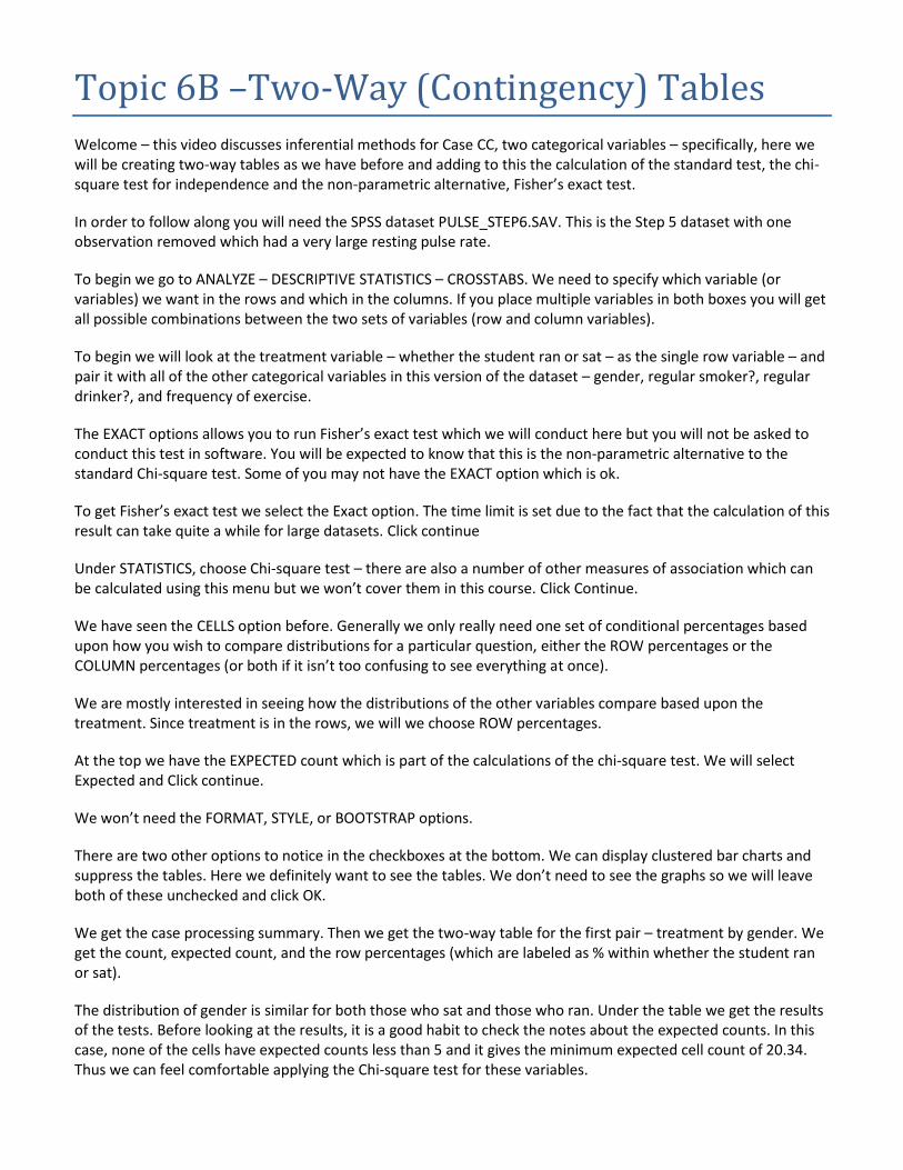
Topic 6B –Two-Way (Contingency) Tables

Welcome – this video discusses inferential methods for Case CC, two categorical variables – specifically, here we will be creating two-way tables as we have before and adding to this the calculation of the standard test, the chi-square test for independence and the non-parametric alternative, Fisher’s exact test.

In order to follow along you will need the SPSS dataset PULSE_STEP6.SAV. This is the Step 5 dataset with one observation removed which had a very large resting pulse rate.

To begin we go to ANALYZE – DESCRIPTIVE STATISTICS – CROSSTABS. We need to specify which variable (or variables) we want in the rows and which in the columns. If you place multiple variables in both boxes you will get all possible combinations between the two sets of variables (row and column variables).

To begin we will look at the treatment variable – whether the student ran or sat – as the single row variable – and pair it with all of the other categorical variables in this version of the dataset – gender, regular smoker?, regular drinker?, and frequency of exercise.

The EXACT options allows you to run Fisher’s exact test which we will conduct here but you will not be asked to conduct this test in software. You will be expected to know that this is the non-parametric alternative to the standard Chi-square test. Some of you may not have the EXACT option which is ok.

To get Fisher’s exact test we select the Exact option. The time limit is set due to the fact that the calculation of this result can take quite a while for large datasets. Click continue

Under STATISTICS, choose Chi-square test – there are also a number of other measures of association which can be calculated using this menu but we won’t cover them in this course. Click Continue.

We have seen the CELLS option before. Generally we only really need one set of conditional percentages based upon how you wish to compare distributions for a particular question, either the ROW percentages or the COLUMN percentages (or both if it isn’t too confusing to see everything at once).

We are mostly interested in seeing how the distributions of the other variables compare based upon the treatment. Since treatment is in the rows, we will we choose ROW percentages.

At the top we have the EXPECTED count which is part of the calculations of the chi-square test. We will select Expected and Click continue.

We won’t need the FORMAT, STYLE, or BOOTSTRAP options.

There are two other options to notice in the checkboxes at the bottom. We can display clustered bar charts and suppress the tables. Here we definitely want to see the tables. We don’t need to see the graphs so we will leave both of these unchecked and click OK.

We get the case processing summary. Then we get the two-way table for the first pair – treatment by gender. We get the count, expected count, and the row percentages (which are labeled as % within whether the student ran or sat).

The distribution of gender is similar for both those who sat and those who ran. Under the table we get the results of the tests. Before looking at the results, it is a good habit to check the notes about the expected counts. In this case, none of the cells have expected counts less than 5 and it gives the minimum expected cell count of 20.34. Thus we can feel comfortable applying the Chi-square test for these variables.

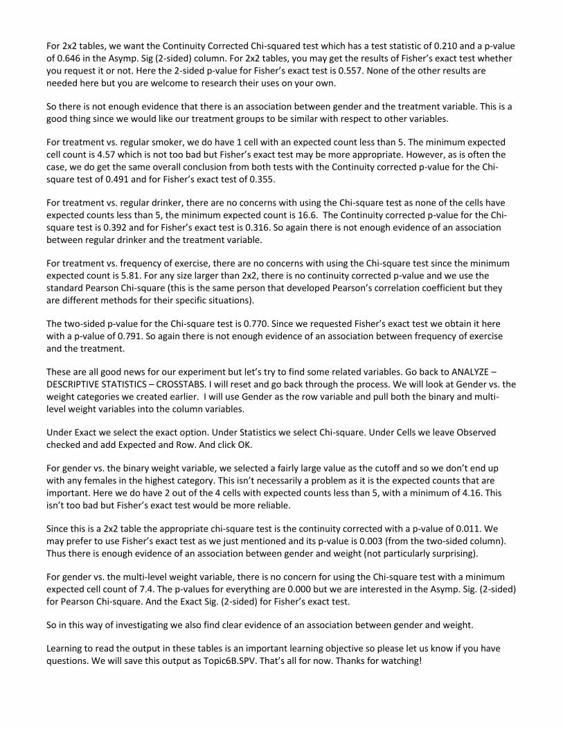
For 2x2 tables, we want the Continuity Corrected Chi-squared test which has a test statistic of 0.210 and a p-value of 0.646 in the Asymp. Sig (2-sided) column. For 2x2 tables, you may get the results of Fisher’s exact test whether you request it or not. Here the 2-sided p-value for Fisher’s exact test is 0.557. None of the other results are needed here but you are welcome to research their uses on your own.

So there is not enough evidence that there is an association between gender and the treatment variable. This is a good thing since we would like our treatment groups to be similar with respect to other variables.

For treatment vs. regular smoker, we do have 1 cell with an expected count less than 5. The minimum expected cell count is 4.57 which is not too bad but Fisher’s exact test may be more appropriate. However, as is often the case, we do get the same overall conclusion from both tests with the Continuity corrected p-value for the Chi-square test of 0.491 and for Fisher’s exact test of 0.355.

For treatment vs. regular drinker, there are no concerns with using the Chi-square test as none of the cells have expected counts less than 5, the minimum expected count is 16.6. The Continuity corrected p-value for the Chi-square test is 0.392 and for Fisher’s exact test is 0.316. So again there is not enough evidence of an association between regular drinker and the treatment variable.

For treatment vs. frequency of exercise, there are no concerns with using the Chi-square test since the minimum expected count is 5.81. For any size larger than 2x2, there is no continuity corrected p-value and we use the standard Pearson Chi-square (this is the same person that developed Pearson’s correlation coefficient but they are different methods for their specific situations).

The two-sided p-value for the Chi-square test is 0.770. Since we requested Fisher’s exact test we obtain it here with a p-value of 0.791. So again there is not enough evidence of an association between frequency of exercise and the treatment.

These are all good news for our experiment but let’s try to find some related variables. Go back to ANALYZE – DESCRIPTIVE STATISTICS – CROSSTABS. I will reset and go back through the process. We will look at Gender vs. the weight categories we created earlier. I will use Gender as the row variable and pull both the binary and multi-level weight variables into the column variables.

Under Exact we select the exact option. Under Statistics we select Chi-square. Under Cells we leave Observed checked and add Expected and Row. And click OK.

For gender vs. the binary weight variable, we selected a fairly large value as the cutoff and so we don’t end up with any females in the highest category. This isn’t necessarily a problem as it is the expected counts that are important. Here we do have 2 out of the 4 cells with expected counts less than 5, with a minimum of 4.16. This isn’t too bad but Fisher’s exact test would be more reliable.

Since this is a 2x2 table the appropriate chi-square test is the continuity corrected with a p-value of 0.011. We may prefer to use Fisher’s exact test as we just mentioned and its p-value is 0.003 (from the two-sided column). Thus there is enough evidence of an association between gender and weight (not particularly surprising).

For gender vs. the multi-level weight variable, there is no concern for using the Chi-square test with a minimum expected cell count of 7.4. The p-values for everything are 0.000 but we are interested in the Asymp. Sig. (2-sided) for Pearson Chi-square. And the Exact Sig. (2-sided) for Fisher’s exact test.

So in this way of investigating we also find clear evidence of an association between gender and weight.

Learning to read the output in these tables is an important learning objective so please let us know if you have questions. We will save this output as Topic6B.SPV. That’s all for now. Thanks for watching!

Topic 7A – Numeric Summaries by Groups

Welcome – this tutorial will cover exploratory data analysis in Case CQ (or QC) where we have one quantitative variable and one categorical variable. Here we will cover calculating numeric measures for the quantitative variable WITHIN EACH LEVEL of the categorical variable using EXPLORE.

In order to follow along you will need the SPSS dataset PULSE_STEP3.SAV (after translating the original coded categorical variables). We have the dataset open in SPSS.

To conduct this analysis we go to ANALYZE – DESCRIPTIVE STATISTICS – EXPLORE. Quantitative variables will go in the dependent list – the same as when we looked at one quantitative variable – the factor list will contain our categorical variable or variables. If multiple variables are placed in both lists you will get all possible combinations of dependent variables with factor variables. We won’t need the Label Cases By option.

We will focus on the resting pulse rate as our quantitative variable and we will use all of our categorical variables as factors (except year).

The settings are the same as for one quantitative variable with STATISTICS – choose percentiles if you wish to see the quartiles.

In PLOTS we will choose histograms and normality plots – this will provide these WITHIN the levels of the factors.

We will not need OPTIONS or BOOTSTRAP.

We can choose whether to obtain the statistics, plots or both – we will choose both and click OK.

This produces a lot of output but it is all useful when you are exploring relationships in Case CQ (or QC). Looking quickly through the boxplots we see that females have a slightly higher resting pulse rate and there is one male with an extreme outlier – could be an error.

Comparing smokers and non-smokers is difficult due to the small sample size for smokers in the data – overall the comparison is less overall variation but this could be a result of the lack of data.

There is more variation among regular drinkers than non-drinkers but the center is about the same.

For exercise, it does seem there is a weak trend that the more you exercise, the lower your resting pulse rate – as we might expect.

And finally for treatment – the groups have a similar distribution of resting pulse rates – we will adjust for initial pulse rate in our analysis but it is still good that our groups were reasonably similar for our Ran and Sat groups to begin with.

The outlier does concern me – so likely I will investigate and possibly remove it in the next set of data manipulations where we will create some new variables.

Finding numerical summaries – as well as many graphical summaries – is very easy using explore. It can be useful for one quantitative variable or for situations such as these involving one quantitative variable and one categorical variable. It should be the first thing you think to do in these cases as it will often provide the capability of obtaining all of the results that you need.

We will save this output as Topic7A.SPV. That’s all for this tutorial. Thanks for watching!

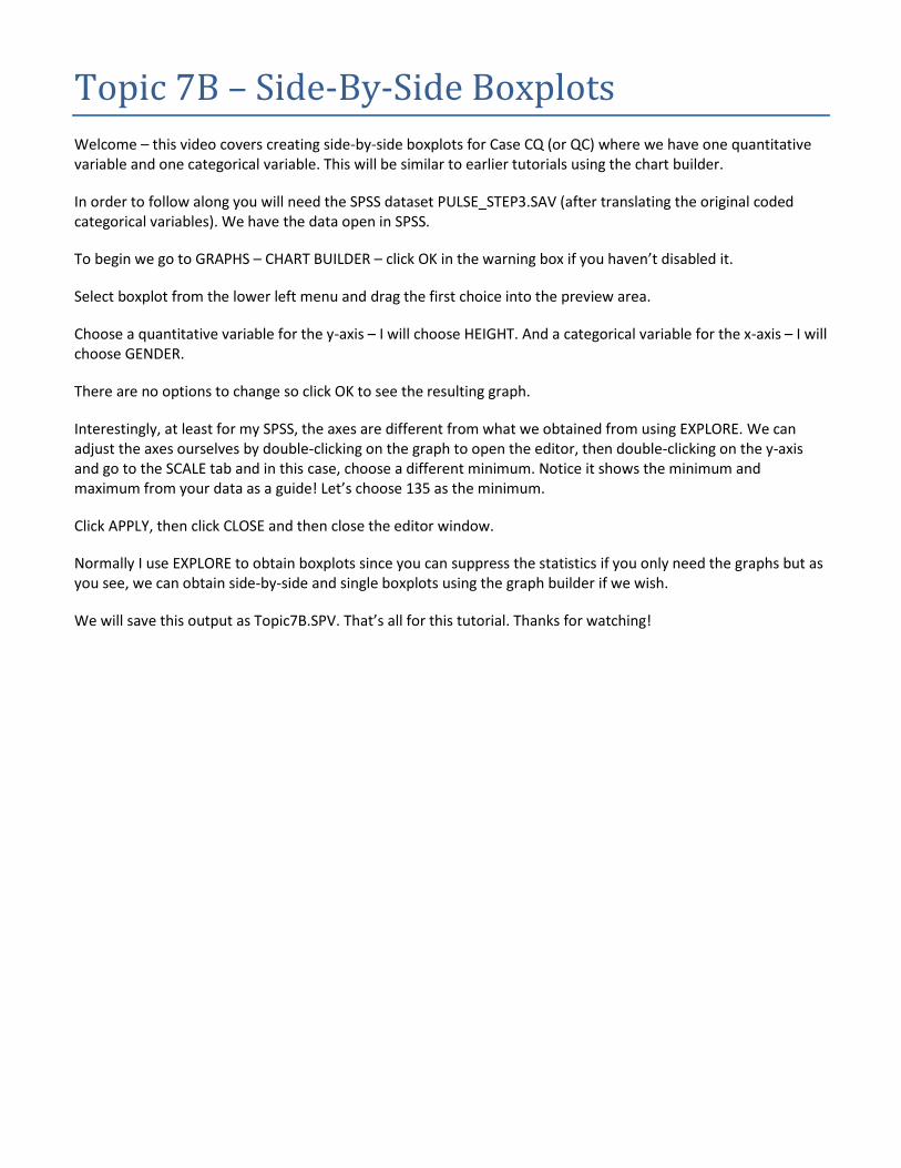
Topic 7B – Side-By-Side Boxplots

Welcome – this video covers creating side-by-side boxplots for Case CQ (or QC) where we have one quantitative variable and one categorical variable. This will be similar to earlier tutorials using the chart builder.

In order to follow along you will need the SPSS dataset PULSE_STEP3.SAV (after translating the original coded categorical variables). We have the data open in SPSS.

To begin we go to GRAPHS – CHART BUILDER – click OK in the warning box if you haven’t disabled it.

Select boxplot from the lower left menu and drag the first choice into the preview area.

Choose a quantitative variable for the y-axis – I will choose HEIGHT. And a categorical variable for the x-axis – I will choose GENDER.

There are no options to change so click OK to see the resulting graph.

Interestingly, at least for my SPSS, the axes are different from what we obtained from using EXPLORE. We can adjust the axes ourselves by double-clicking on the graph to open the editor, then double-clicking on the y-axis and go to the SCALE tab and in this case, choose a different minimum. Notice it shows the minimum and maximum from your data as a guide! Let’s choose 135 as the minimum.

Click APPLY, then click CLOSE and then close the editor window.

Normally I use EXPLORE to obtain boxplots since you can suppress the statistics if you only need the graphs but as you see, we can obtain side-by-side and single boxplots using the graph builder if we wish.

We will save this output as Topic7B.SPV. That’s all for this tutorial. Thanks for watching!

Topic 7C – Two Independent Samples T-test

Welcome – this video covers the two-sample t-test for independent samples. This test will compare the mean of a quantitative variable for the two groups defined by a binary categorical variable which falls into Case CQ.

In order to follow along you will need the SPSS dataset PULSE_STEP6.SAV. Here we will start by looking at how resting pulse rates compared between the two treatments. Hopefully we have relatively comparable groups from the beginning.

Go to ANALYZE – COMPARE MEANS – INDEPENDENT SAMPLES T-TEST. For the test variable, we will choose Resting Pulse rate and for the grouping variable, we choose the treatment variable – whether the student ran or sat.

Now we must define our groups based upon the raw data. Here 1 represents ran and 2 represents sat. We can compare in either direction but we must be careful to interpret the results correctly. Since we hope to not find any significant differences and we expect no particular direction, it really makes no difference here. I will enter 1 for group 1 and 2 for group 2. Click OK to see the results.

For the two-sample t-test, our first decision is whether or not we feel comfortable assuming equal variances. The test for equal variances has a null hypothesis that the variances are equal and an alternative that they are not equal. The p-value is under “Levene’s test for equality of variances” under the Sig. column. Here the p-value for the test of equal variances is 0.480 and so we fail to reject the null hypothesis.

Although we cannot prove the null hypothesis is true, we do not have enough evidence that they are different. This seems reasonable given that the standard deviation of the resting pulse rates for those who Ran is 11.384 and for those who Sat is 10.309. Although there may be a difference it is not statistically significant and any difference that may exist would likely be too small to have a big impact on the results of the t-test.

Thus we will continue with the t-test where equal variances are assumed. This is the first row in the output. The t-statistic is -0.74 and the two-sided p-value is 0.461. Thus there is not enough evidence that the mean resting pulse rate differs between the two treatment groups.

We can see that the confidence interval ranges from -5.779 to 2.638 which included zero and thus we cannot show a statistically significant difference. This is good in that we would like our two groups to be similar with respect to resting pulse rates.

Now we will look at an example where we will be able to find a significant difference. Go to ANALYZE – COMPARE MEANS – INDEPENDENT SAMPLES T-TEST. For the test variable, we will choose Weight and for the grouping variable, we choose Gender.

Now we must define our groups based upon the raw data. Here 1 represents Male and 2 represents Female. We expect males to weight more than females and so it may be easier to look at Males – Females for this analysis as this should give positive values which are easy to interpret. We will choose 1 for Group 1 (this will be Males) and 2 for group 2 (for females). Click OK to see the results.

Again, our first decision is whether or not we feel comfortable assuming equal variances. Here the p-value for the test of equality of variances is 0.000 (in the Sig. Column under Levene’s test). So there is evidence that the variances of the two groups are different. From the summary table this seems reasonable as the standard deviation for males is 14.3 and that for females is 8.5.

Thus we need to use the t-test which does not assume equal variances which is the 2nd row in the table. The test-statistic is 7.915 and the p-value is 0.000 in the Sig. (2-tailed) column under the t-test for equality of means. Thus there is a highly statistically significant difference in the mean weight between males and females.

The confidence interval ranges from 13.341 to 22.276. Since these are calculated as Group 1 (Males) minus Group 2 (Females) we can interpret this by saying we are 95% confident that the mean weight among males is between 13.341 and 22.276 kg greater than that for females.

We will save this output as Topic7C.SPV. That’s all for this tutorial. Thanks for watching!

Topic 7D – One-Way ANOVA (Analysis of Variance)

Welcome – this video covers the one-way ANOVA. This test compares the means of a quantitative variable for the groups defined by a categorical variable. The groups must be independent samples.

For example, we cannot use this to look at multiple measurements taken on the same individual over time as the same person would be reflected in each group and the measurements in one group and those in another would be dependent, not independent. Although it can be used for two-groups, in that case we will use always the two-independent samples t-test in this course.

In order to follow along you will need the SPSS dataset PULSE_STEP6.SAV. Here we will start by looking at the relationship between height and the multi-level weight groups we created in an earlier tutorial.

Go to ANALYZE – COMPARE MEANS – ONE-WAY ANOVA. We drag Height into the dependent list and Weight Categories into the Factor list. For this course, we can stop here and click OK but I will show you how to get the comparisons which are often of interest in practice so that we can identify which groups are statistically significantly different.

Under Post Hoc, two common methods used are Bonferroni and Tukey. These methods adjust for the fact that there are multiple comparisons being made simultaneously and they control the overall Type I error rate at 5% instead of standard confidence intervals which would each have a 5% individually and thus overall the Type I error rate would likely be higher than 5% if we used the standard intervals to determine which groups are significantly different.

Under Options you can also choose things such as descriptives or the test for homogeneity of variances (tests for equal variances). There is also a plot of the means to compare. You are welcome to investigate these on your own but we will cancel without selecting any of these options. Click OK.

For this course, we are primarily interested in the main ANOVA table. It is unfortunate that SPSS does not show us the name of the categorical variable used. Here it was our 5-level weight categories. The p-value is 0.000 in the Sig. column and so there is enough evidence that the mean height is different among some of the weight categories.

The Tukey and Bonferroni output provides the differences in mean height for all possible combinations of weight groups. It gives the difference and denotes whether or not it is statistically significant with a *. It gives the standard error of the difference, the p-value, and the confidence interval to compare the two groups. There are some groups which are not statistically significantly different but many of them are.

With Tukey we get another summary table which provides information about which groups are similar. So Weight category <55 is different from all others and 80+ is also different from all others. But the three middle groups are not statistically different from each other.

Now we will run through that one more time to compare the mean Age between the 5 weight groups. Go to ANALYZE – COMPARE MEANS – ONE-WAY ANOVA. Reset the tool. We drag Age into the dependent list and Weight Categories into the Factor list. We will not select any Post-hoc tests. Click OK.

We see that the p-value is 0.380 and thus there is not enough evidence that the mean age is different among any of the 5 weight groups.

We will save this output as Topic7D.SPV. That’s all for this tutorial. Thanks for watching!

Topic 7E – Non-Parametric Tests for Case CQ

Welcome – this video covers the non-parametric alternatives to the two-independent samples t-test and one-way ANOVA. We will cover the alternative to the paired t-test in a different tutorial.

These tests compare the median of the quantitative variable instead of the mean. If the distributions in the groups are symmetric then this could also be considered a test for the means but not in the case of skewed distributions.

One assumption is that there is only a location shift between the groups. This can limit the usefulness of this test in practice and we should check to see if the distributions are similar using side-by-side boxplots or other graphical displays. We must also remember though that this assumption is about the population and so small deviations are not likely a problem but major differences would be.

We will look at Height vs. gender, Height vs weight categories and Age vs. weight categories.

All of these have relatively similar distributions. The relatively minor differences seen in the shapes could be due to chance. Thus these tests are reasonable.

We begin with the Wilcoxon Rank-Sum test, also known as the Mann-Whitney U-test. This is for two groups and is analogous to the two independent samples t-test.

Go to ANALYZE – NON-PARAMETRIC TESTS – INDEPENDENT SAMPLES. Some students may not have this option depending on the version of SPSS but we are illustrating it for those students who are interested in conducting these tests in practice.

You can let SPSS make some default choices based upon the data types but we will go through how to request this specific test. So we will choose Customize Analysis. Then go to the Fields tab. Here we drag the response variable into the Test Fields list. We choose height. We drag gender into the groups.

Then go to the Settings tab and choose customize tests and select Mann-Whitney U (2 samples). Then click Run.

This provides a simple summary with the p-value of the test which here is 0.000 and it gives the decision, which here is to reject the null hypothesis. Thus there is enough evidence that median height is different between males and females.

Now we will look at the Kruskal-Wallis test which is analogous to the One-Way ANOVA. We will look height and age vs. weight categories.

Go to ANALYZE – NON-PARAMETRIC TESTS – INDEPENDENT SAMPLES. Reset the tool. Under the Objective tab, choose customize analysis. Under fields, drag height and age into the test fields list. Drag weight categories into groups. Under the settings tab choose customize tests and the Kruskal-Wallis for k-samples. Then click Run.

Not surprising, the test finds that some medians are statistically significantly different between the weight categories for height but not for age. This seems reasonable given the boxplots.

We will save this output as Topic7E.SPV. That’s all for this tutorial. Thanks for watching!

Topic 8A – Setting up Data for Paired T-test

Welcome – this video will modify the current dataset so that we can conduct a paired t-test for each of our two treatment groups. We want to conduct a test to determine if the mean pulse rate changes among those who ran and again, another test for those who sat.

In order to follow along you will need the SPSS dataset PULSE_STEP6.SAV.

To begin we will calculate the differences between pulse2 (after the treatment) and pulse 1 (before the treatment). We will expect an increase for those who ran and basically no difference for those who sat.

To do this we go to TRANSFORM – COMPUTE VARIABLE. We name the new variable Diff_2v1 to remind ourselves that we are calculating Pulse 2 – Pulse 1. Then drag Pulse 2 into the numeric expression box and then minus and drag Pulse 1 into the box. Then click OK.

Review the data to make sure everything looks good, and it does. In the Variable view we will provide a variable label of DIFF (Pulse2 – Pulse1).

We will save this dataset as PULSE_STEP7.SAV.

Now we want to split this dataset into two datasets. One for each treatment. To do this we will go to DATA – SELECT CASE. Choose “If condition is satisfied” and click on IF. We want to select those who ran which have a value of 1 for that variable. We drag that variable into the box and then = 1 and click continue.

We will select copy selected cases to a new dataset and name this dataset PulseSplit_Ran. And click OK. Go to the untitled dataset and save this file again as PulseSplit_Ran. The name we gave before was internal.

Now we repeat that process for TRT = 2 and save the resulting dataset as PulseSplit_Sat.

That’s all for this tutorial. Thanks for watching!

Topic 8B – Exploratory Analysis of Difference

Welcome – this video will investigate the differences in pulse rates using explore. In SPSS we may need to do this in order to investigate the assumptions of the paired t-test even though we can conduct the test without calculating the differences ourselves.

In order to follow along you will need the SPSS dataset PULSESPLIT_RAN.SAV. A similar process could be used for the dataset for those who SAT.

We begin by going to ANALYZE – DESCRIPTIVE STATISTICS – EXPLORE. Drag in the differences into the dependent list. Under statistics you can choose percentiles or other options as needed but we will leave the default.

Under plots, we will select histogram and normality plot with tests and click continue and then click OK.

We might be mostly interested in the QQ-plot to see if normality is reasonable, especially for small sample sizes. We can see that the data do appear to be reasonably normally distributed since the observed values fall close to the line of values representing the expected values for a normal distribution.

The histogram also looks reasonably normally distributed. The median is off center in the boxplot but overall the distribution seems reasonably normal based upon these plots.

We might also be interested in the numerical summaries in practice to describe these differences further.

We will save this output as Topic8B.SPV. That’s all for this tutorial. Thanks for watching!

Topic 8C – Paired T-test

Welcome – this video will conduct the paired t-test. There are a few ways we can do this. Generally you only need to do one of these for any requested analyses in this course.

In order to follow along you will need the SPSS datasets PULSESPLIT_RAN.SAV. A similar process could be used for the dataset for those who SAT.

We begin by going to ANALYZE – COMPARE MEANS – PAIRED T-TEST. In this method, SPSS will calculate the differences for us. We can decide which way we wish to calculate the differences by which order we provide the variables. Here we will put the after treatment pulse in variable 1 and the before in variable 2. This will calculate the differences as Pulse2 minus Pulse1.

If you wish to swap the choice you can land on either variable and then click on the left-right arrow on the bottom of the right side.

When you are happy with your choice, click OK.

This provides the results for the paired t-test including a summary of each group and the correlation between the before and after measurements. Although linear regression can be done in this case – it is not usually of primary interest, instead a test of the differences is more of interest than predicting the after pulse rate using the before pulse rate.

Not surprising, in the last table, we find the p-value of the paired t-test is 0.000 indicating there is a statistically significant difference in the mean pulse rate before and after treatment among those who Ran. The confidence interval suggests with 95% confidence that the mean pulse rate after treatment among those who ran is between 46.1 and 58.7 beats faster than the mean pulse rate before treatment.

Alternatively we can use the one-sample t-test directly on the differences. To do this we go to ANALYZE – COMPARE MEANS – ONE-SAMPLE T-test. This same tool would also be used for any other general one-sample t-test not just paired t-tests.

We will drag the differences we calculated in an earlier tutorial into the test variable list. For this paired t-test we will set the test value to 0 which is the default. If we were interested in testing the mean for a general variable we would need to put the appropriate value into this box.

Click OK. The p-value and confidence interval are identical but now our summary at the top is on the differences instead of each individual variable.

We will save this output as Topic8C.SPV. That’s all for this tutorial. Thanks for watching!

Topic 8D – Non-Parametric Alternative

Welcome – this video will conduct the non-parametric alternatives to the paired t-test. There are two possible tests. The Sign-test which is based only on whether or not each difference is positive, negative, or zero and the Wilcoxon Signed-Rank test which is based upon the ranks of the positive and negative differences.

In order to follow along you will need the SPSS dataset PULSESPLIT_RAN.SAV. A similar process could be used for the dataset for those who SAT.

We have two ways to conduct these tests – based upon the differences we calculated using one-sample results or based upon the actual pulse measurements using dependent sample methods.

We begin by going to ANALYZE – NON-PARAMETRIC TESTS – RELATED SAMPLES. In this method, SPSS will calculate the differences for us. We will choose Customize analysis in the Objective tab. In the Fields tab we select our two pulse variables and pull them into the test fields box. Under settings choose Customize tests. We will select both the sign test and Wilcoxon matched pair signed-rank. And click Run.

This provides two results, both of which indicate there are highly statistically significant differences in the median pulse rate when comparing before and after. We don’t get any more details and would need to look at the data to describe more about these differences.

Now we go back to ANALYZE – NON-PARAMETRIC TESTS and now choose ONE-SAMPLE. In this method, we need to have the differences already calculated in our dataset. We will choose Customize analysis in the Objective tab. In the Fields tab, for some reason in my SPSS all of the variables are automatically selected which we do not want. I remove them all and then select our difference variable and pull it into the test fields box.

Under settings choose Customize tests. We will select both the binomial test (which is the sign test for one sample) and Wilcoxon signed-rank. For the binomial test, click on options. We need to select a custom cutpoint of 0 and click OK. And under the Wilcoxon test we need to type 0 into the hypothesized median box. And click Run.

The results are the same as those obtained using the related samples method.

We will save this output as Topic8D.SPV. That’s all for this tutorial. Thanks for watching!

Topic 9A – Basic Scatterplots

Welcome – this video covers creating scatterplots in Case QQ where we have two quantitative variables. This will be similar to earlier tutorials using the chart builder.

In order to follow along you will need the SPSS dataset PULSE_STEP3.SAV (after translating the original coded categorical variables). We have the data open in SPSS.

To begin we go to GRAPHS – CHART BUILDER – click OK in the warning box if you haven’t disabled it.

Select scatter/dot from the lower left menu and drag the first choice into the preview area.

Choose a quantitative variable for the each axis. Let’s predict weight (Y) using height (X).

There are no options to change so click OK to see the resulting graph. Here we see our scatterplot showing that, not surprisingly, as height increases, weight also tends to increase.

We can add various models to the scatterplot. The two we are most interested in are a LOESS line which is a running average and a linear model from a simple linear regression.

To add these we double-click on the graph to open the editor and click on the “Add Fit Line at Total” selection from the elements menu (or the image in the toolbar that looks like a line).

The linear model is selected by default but let’s begin by changing this to LOESS and click APPLY and CLOSE and close the editor. This is the curve of best fit based upon the data. There are different levels of smoothing which can be chosen by deciding what percentage of points to use to fit the model.

Let’s recreate the scatterplot by going back to GRAPHS – CHART BUILDER and clicking OK to recreate the graph. Double-click on the graph to open the editor, click on the Add Fit Line at Total, and leave the linear default. Click CLOSE and close the editor.

The LOESS line helps us see the trend is slightly non-linear. A linear model will be a somewhat reasonable approximation but a more complex model would likely fit the data better.

We will save this output as Topic9A.SPV. That’s all for this tutorial on basic scatterplots. Thanks for watching!

Topic 9B – Grouped Scatterplots

Welcome – this video covers creating grouped scatterplots using the chart builder. This is actually not part of any of the formal cases we cover in this course as it looks at two quantitative variables and one categorical variable simultaneously. However, these graphs are potentially useful in practice and we do briefly mention them in the course materials.

In order to follow along you will need the SPSS dataset PULSE_STEP3.SAV (after translating the original coded categorical variables). We have the data open in SPSS.

To begin we go to GRAPHS – CHART BUILDER – click OK in the warning box if you haven’t disabled it.

Select scatter/dot from the lower left menu and drag the second choice into the preview area.

Choose a quantitative variable for the each axis. Let’s predict weight (Y) using height (X). Choose one categorical variable for the Set Color box in the upper right corner. We will use GENDER. Then click ok. Let’s go ahead and repeat that two more times to get three copies.

For the first graph we will leave it alone but notice that the males and females do cluster together – you can change the colors and symbols to help clarify the graph if needed.

For the second, double-click on the graph to open the editor and click on the “Add Fit Line at Subgroups” selection from the elements menu (or the image in the toolbar that looks like two lines).

The linear model is selected by default but let’s begin by changing this to LOESS and click APPLY and CLOSE and close the editor. This shows that, as we would expect, the males and females do cluster together and gives the best guess at the trend based upon the data within each group. We can see that on average, the slope seems to be a little steeper for males than females.

For the third graph, double-click on the graph to open the editor, click on Add Fit Line at Subgroups, leave the default linear setting, click close and then close the editor. This gives the linear regression equations for each gender. To get the best predictions, we may need to have a model for males and a model for females.

Grouped scatterplots with trend-lines can definitely help us investigate more complex trends in our data.

We will save this output as Topic9B.SPV. That’s all for tutorial on grouped scatterplots. Thanks for watching!

Topic 9C – Pearson’s Correlation Coefficient

Welcome – this video covers calculating Pearson’s correlation coefficient for Case QQ where we have two quantitative variables which are linearly related. Everything we need to learn about this procedure in this course will be covered in this tutorial.

In order to follow along you will need the SPSS dataset PULSE_STEP3.SAV (after translating the original coded categorical variables). We already have the data open in SPSS.

To begin we go to ANALYZE – CORRELATE – BIVARIATE.

We should verify that the relationship is reasonably linear using a scatterplot before conducting this analysis. The correlation will be calculated for all pairs of variables which are placed in the variables list.

We looked at height and weight earlier and found that, although it is best to analyze within each gender, the data are only slightly non-linear when considered together. This will give a measure of the strength and direction of the simple linear regression model through this data.

Drag height and weight into the variables area.

In OPTIONS, you can decide whether or not to obtain means and standard deviations. We are not interested in the option for cross-product deviations and covariances in this course. I will check the box for means and standard deviations to show the results.

We don’t need anything in STYLE or BOOTSTRAP.

For now we are interested in Pearson’s correlation so leave that box checked. Later we will discuss Spearman’s rank correlation which can be obtained by checking the Spearman box – for now we will leave it unchecked.

The remaining options relate to the inferential component for correlations – we will leave these settings at their default throughout the course but if you ever decide you do not want significant correlations flagged, you can uncheck that last box. Click OK to see the results.

Since we asked for means and standard deviations, we get this first table with descriptive statistics.

Then we get the correlations themselves. Many students find this difficult to read at first. The correlation we need is 0.741 in this case, the value in the Pearson correlation row - between height and weight in row 1 - or between weight and height in row 2. It repeats for both combinations even though the values are the same – a little strange but standard in most statistical packages.

The next row is the significance which we will learn later is the p-value to determine if this correlation is statistically significantly different from zero. Is there a statistically significant correlation between height and weight? We don’t have to be statisticians to know that there is but we will discuss the details later in the course.

The double stars ** denote that the correlation is significant at the 0.01 level as indicated in the note below the table – this is the result of flagging significant correlations.

Then we get the sample size, N. Let’s save this output as Topic9C.SPV.

You might try running this on many quantitative variables to see what happens. We will show that result later! That’s all for this tutorial on calculating Pearson’s correlation coefficient. Thanks for watching!

Topic 9D – Simple Linear Regression - EDA

Welcome – this video covers calculating the simple linear regression equation for Case QQ where we have two quantitative variables which are linearly related.

In order to follow along you will need the SPSS dataset PULSE_STEP3.SAV (after translating the original coded categorical variables). We already have the data open in SPSS.

To begin we go to ANALYZE – REGRESSION – LINEAR.

We should verify that the relationship is reasonably linear using a scatterplot before conducting this analysis.

We looked at height and weight earlier and found that, although it is best to analyze within each gender, the data are only slightly non-linear when considered together. This will calculate the values needed for the simple linear regression equation for this data.

For regression, we must be careful to put the Y variable – outcome or response – into the dependent variable list and the X variable – predictor or explanatory – into the independent list. Generally we will conduct only one regression at a time in this course.

Drag weight into the Dependent area and height into the independent area.

When we return for the inferential statistics component, we will make some changes in STATISTICS and PLOTS and discuss the SAVE option but for now we will not make any changes in these settings.

We don’t need anything in OPTIONS, STYLE or BOOTSTRAP.

Click OK to see the results.

By default we obtain 4 tables. The only one we are concerned with at this point is the very last. We need to find the slope and intercept of the linear regression equation. In SPSS these are labeled as B under the UNSTANDARDIZED COEFFICIENTS columns.

The row labeled CONSTANT is the INTERCEPT, here it is negative 121.173.

The row labeled with the x-variable label – in this case Height (cm) – is the SLOPE, here it is 1.085.

So the regression equation would be Y-hat = -121.173 + 1.085(HEIGHT).

The slope implies that on average, for each 1 cm increase in height the mean weight increases by 1.085 kg.

We will save this output as Topic9D.SPV.

Later we will discuss the ANOVA table and the interpretation of R-square in the Model summary table but for now that’s all we need for simple linear regression. Thanks for watching!

Topic 9E – Simple Linear Regression - Inference

Welcome – this video covers calculating the simple linear regression equation for Case QQ where we have two quantitative variables which are linearly related as well as looks at the inferential components.

In order to follow along you will need the SPSS dataset PULSE_STEP3.SAV. We already have the data open in SPSS.

To begin we go to ANALYZE – REGRESSION – LINEAR.

We should verify that the relationship is reasonably linear using a scatterplot before conducting this analysis.

We looked at height and weight earlier and found that, although it is best to analyze within each gender, the data are only slightly non-linear when considered together. This will calculate the values needed for the simple linear regression equation for this data.

For regression, we must be careful to put the Y variable – outcome or response – into the dependent variable list and the X variable – predictor or explanatory – into the independent list. Generally we will conduct only one regression at a time in this course.

Drag weight into the Dependent area and height into the independent area.

In STATISTICS, add to the estimates and model fit, the confidence intervals. You can also select descriptives if you wish. Click continue.

In PLOTS, we want to create a few plots of the residuals. The first two are easy, we simply select the two checkboxes for histogram and normal probability plot. This is different from a QQ-plot but provides a similar way of checking for normality and getting the QQ-plot would require us to export the residuals and then explore them in the way we learned for one quantitative variable. This is possible but not necessary.

The other plot we must create. We pull the ZRESID into the Y area and ZPRED into the X area. You can create additional plots by clicking next. Click continue when you have these three plots requested.

The SAVE option does allow you to save the residuals into your dataset and explore them further but we will not do that here.

We don’t need anything in OPTIONS, STYLE or BOOTSTRAP.

Click OK to see the results.

Since we asked for the descriptives, we get the summary statistics for our two variables. We also get the correlation. Notice that here we obtain the 1-tailed p-value – be careful as for results in this course, we want the two-sided p-value given by using CORRELATE instead.

Then there is some information about the variables entered/removed. This is more for multiple regression which is beyond the scope of our course.

Then we have the model summary. Of interest here is the R-square value of 0.550. This can be interpreted by saying that this model using height explains 55% of the variation in weight.

Then we get the overall ANOVA table. Regression and analysis of variance are mathematically the same process but the one-way ANOVA is a special case as is simple linear regression.

This table provides an overall p-value of whether the model explains a significant amount of variation. In this case, the overall p-value is 0.000 and thus this model does explain a significant amount of the variation in weight.

Then we get a table of the coefficients which we have seen before. Here we have added the confidence intervals for the parameter estimates. If the intercept is meaningful then this may be of interest but in this case, the intercept represents the mean weight for someone with a height of zero which is not possible in practice.

The confidence interval for the slope is of interest as this provides bounds for the increase or decrease in the mean response for each 1-unit increase of the explanatory variable.

The row labeled CONSTANT is the INTERCEPT, here it is negative 121.173.

The row labeled with the x-variable label – in this case Height (cm) – is the SLOPE, here it is 1.085.

So the regression equation would be Y-hat = -121.173 + 1.085(HEIGHT).

The slope implies that on average, for each 1 cm increase in height the mean weight increases by 1.085 kg and the 95% confidence interval suggests this increase could be as low as 0.895 to as high as 1.275.

Finally there is a summary of the residual statistics.

For the graphs, we get a histogram of the residuals with a normal curve overlay. We want the residuals to be normally distributed which by this graph they seem to be.

Then we get a Normal P-P plot of the residuals which is similar to but scaled very differently than the QQ-plot. It will always match at the endpoints. We are still looking for the points to follow the line in order to be able to say the plot is reasonably normally distributed which they do here.

Finally we get the scatterplot of the residuals on the y-axis vs. the predicted values on the x-axis. We are looking for a random scatter of relatively equal spread around the center regardless of the location on the x-axis. If we see any pattern it can indicate non-linearity or non-constant variance depending on the type of pattern. Both of these issues are violations of the assumptions of this method. The more harsh the violation, the more concern we would have.

In this case there is some evidence of non-constant variance in that for large values on the x-axis there seems to be more variation. Possibly we have two clusters illustrating the different genders. We could investigate further by analyzing the two genders separately.

We will save this output as Topic9E.SPV. That’s all for now. Thanks for watching!