Spatial analysis of epidemics: Disease patterns - CFAES analysis of epidemics: Disease patterns...

Spatial analysis of epidemics: Disease patternsEverything is related to everything else, but near things are more related than distant things

--Tobler (1970) (Tobler's 'Law of Geography')

A different perspective Consider the: arrangement of diseased individuals with each

other and with their physical surroundings -- pattern or dispersion

Generally studied separately from disease gradients○ For practical purposes, gradients are typically studied when there is one

(original) inoculum source○ Patterns are typically studied where there are "many" or an undefined

number of inoculum sources

The approach (spatial pattern analysis) is very statistical (stochastic) in nature○ In contrast, for gradients (and disease progress curves), the basic

approaches were mostly based on deterministic models (either for Y, or dY/ds, or dy/ds, or y/s), and statistical versions of models were used primarily for parameter estimation

Epidem12_13_

Epidem12_13_ Page 2

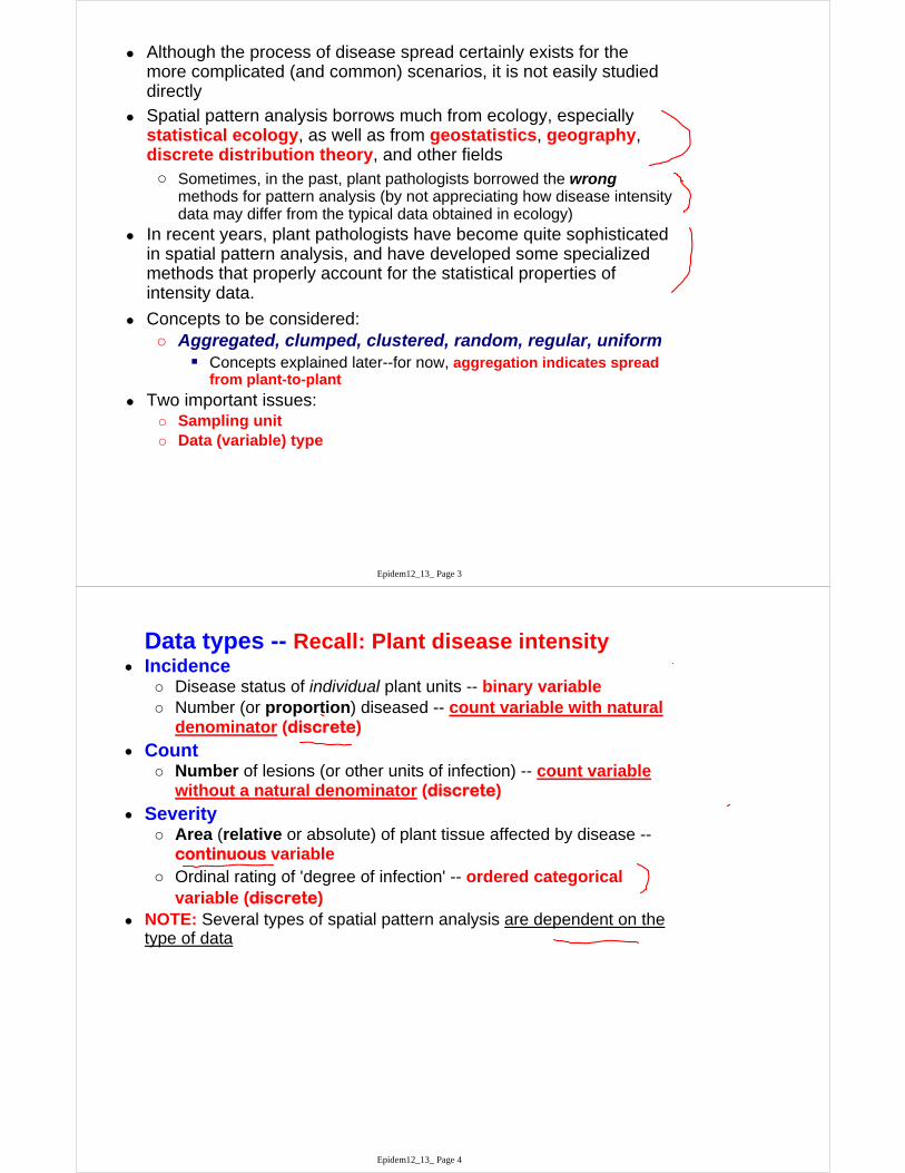
Although the process of disease spread certainly exists for the more complicated (and common) scenarios, it is not easily studied directly

Spatial pattern analysis borrows much from ecology, especially statistical ecology, as well as from geostatistics, geography, discrete distribution theory, and other fields○ Sometimes, in the past, plant pathologists borrowed the wrong

methods for pattern analysis (by not appreciating how disease intensity data may differ from the typical data obtained in ecology)

In recent years, plant pathologists have become quite sophisticated in spatial pattern analysis, and have developed some specialized methods that properly account for the statistical properties of intensity data.

Concepts to be considered:○ Aggregated, clumped, clustered, random, regular, uniform

Concepts explained later--for now, aggregation indicates spread from plant-to-plant

Two important issues:○ Sampling unit○ Data (variable) type

Epidem12_13_ Page 3

Data types -- Recall: Plant disease intensity Incidence

○ Disease status of individual plant units -- binary variable○ Number (or proportion) diseased -- count variable with natural

denominator (discrete)

Count○ Number of lesions (or other units of infection) -- count variable

without a natural denominator (discrete)

Severity○ Area (relative or absolute) of plant tissue affected by disease --

continuous variable○ Ordinal rating of 'degree of infection' -- ordered categorical

variable (discrete) NOTE: Several types of spatial pattern analysis are dependent on the

type of data

Epidem12_13_ Page 4

Sampling Unit (SU):○ The entity to be observed or measured (i.e., entities to be sampled)

Leaf, branch (shoot), plant, group of plants, field Each SU can consist of one or multiple individuals (single leaves,

leaves on a tree)Sample: ○ A selection from a larger population (a collection of sampling units)

We use N for number of sampling units○ Chosen in various ways (randomly, systematically, etc.)○ Cluster sampling:

If each sampling unit (e.g., plant) consists of n individuals (e.g., leaves), and observations are made on all n individuals (n > 1)□ i.e., there is more than one individual observed per sampling unit

Note: there is a total of n·N individuals in the full sample Disease may or may not be clustered with cluster sampling!

Census:○ Observation of all individuals (and obviously all sampling units) in the

population All plants in a field (if the plants in the field are the only ones of interest)

○ We still use sampling unit with a census Think of the field as representative of a super-population

Epidem12_13_ Page 5

Data collection: sparse sampling versus intensive mapping Sparse sampling:

○ Only the observation or measurement (e.g., disease status of plant, number of diseased plants) is recorded for a generally restricted number of sampling units

○ Spatial location of the sampling unit is not recorded or known○ Spatial analyses require discrete data! And, statistical methods

appropriate for discrete data. (binary, counts [with or without a natural denominator]) Indicate heterogeneity (variability) of disease intensity

□ Just one aspect of pattern Intensive mapping:

○ Both the observation (or measurement) and spatial location are recorded for the sampling units (sampling with 'spatially-referenced' sampling units) Distances between sampling units can be determined and utilized Often, a large number of sampling units

○ Allows mapping of observations (for the results of each sampling unit, not necessarily for each observation within the sampling units)

○ Analyses for both discrete and continuous data○ Indicate pattern over many scales (ultimately)

Epidem12_13_ Page 6

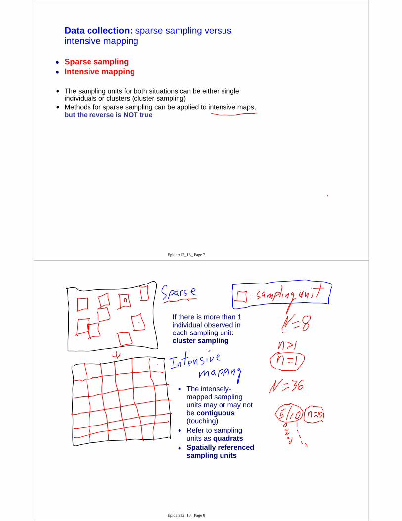
Data collection: sparse sampling versus intensive mapping

Sparse sampling Intensive mapping

The sampling units for both situations can be either single individuals or clusters (cluster sampling)

Methods for sparse sampling can be applied to intensive maps, but the reverse is NOT true

Epidem12_13_ Page 7

The intensely-mapped sampling units may or may not be contiguous (touching)

Refer to sampling units as quadrats

Spatially referenced sampling units

If there is more than 1 individual observed in each sampling unit: cluster sampling

Epidem12_13_ Page 8

Spatial pattern analysis○ Large field of study○ We will focus on just a few situations...

Discrete data: counts with natural denominator□ That is, disease incidence (either as the count itself,

or proportion) is determined for each sampling unit□ Sampling unit consists of n individuals

That is, cluster sampling is used (with N"clusters" or sampling units)

□ Either sparse sampling or intensive mapping□ Probably the most common situation

○ Book (chapter 9) gives details on: Binary data (incidence) -- that is, not cluster sampling Count data (without natural denominator)

□ Example: Number of lesions, …, number of spores, ... Most common situation in ecology, entomology, and

other fields

Epidem12_13_ Page 9

Why study patterns?

Infer the nature of pathogen dispersal or disease spread (spread from plant to plant? Spatial range of inoculum dispersal?○ Here, observed pattern itself is of interest (various statistics can

indicate the range of dispersal) Pattern is the response variable

Properly estimate mean disease intensity and the variability of disease intensity--SAMPLING ○ Determine the required number of sampling units to:

Achieve a certain precision, or to Obtain a decision tool with low probability of false positives and

false negatives○ Here, pattern is of interest only because pattern affects standard

errors of parameter estimates (sampling distributions of the parameter estimates)

Determine how pattern affects disease development○ Here, the pattern is the 'treatment' (dy/dt is the response)

Determine how disease development affects pattern○ Here, pattern is the response variable

Epidem12_13_ Page 10

Analysis of sparsely-sampled incidence data

Cluster samples (so that there are n individuals observed in each sampling unit)

Total of N sampling units Y is number of diseased individuals (say, for the entire sample) Yi is number of diseased individuals in the i-th sampling unit yi is the proportion of diseased individuals in the i-th sampling unit (=Yi / n)

Mean proportion is an estimate of probability of a plant (or plant unit [e.g., leaf]) being diseased (p)

Be careful: don't confuse lower and upper case



Random pattern (for discrete data): The probability of a plant (or plant unit [e.g., leaf]) being

diseased is independent of the disease status of other plants ○ That is, p is constant (across SUs)

The disease status of a plant is unrelated to disease status of neighboring plants (correlation of disease status of a given plant with neighboring plants is zero)

Knowing the disease status of a plant provides no information on the disease status of other plants

If p is constant, diseased individuals per sampling unit (Y) has a binomial distribution

Distribution, or probability distribution:○ (For discrete random variables): a mathematical

formula that gives the probability of each value of the variable

Distributions are evaluated by comparing the observed frequency (O) of diseased individuals to predicted (expected; E) frequency


0 1 2 3 4 5 6 7 8 9 10 11 12 13

Diseased leaflets per sampling unit

0

4

8

12

16

Fre

quen

cy

Obs.

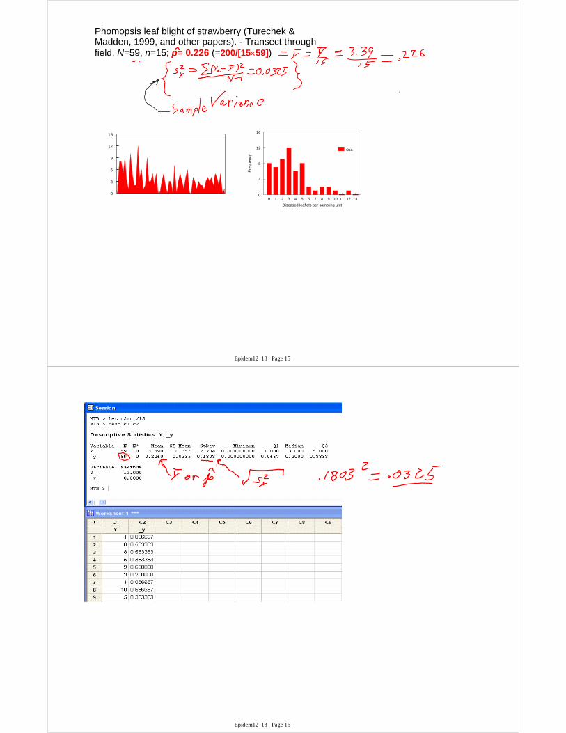
Phomopsis leaf blight of strawberry (Turechek & Madden, 1999, and other papers). - Transect through field. N=59, n=15; p= 0.226 (=200/[1559])

12345678910111213141516171819202122232425262728293031323334353637383940414243444546474849505152535455565758590

3

6

9

12

15

1 8 8 5 9 3 1 10 5 22 12 4 6 1 2 9 3 3 52 5 0 0 3 5 2 0 3 30 7 0 3 5 3 1 4 6 00 4 3 1 3 2 2 1 3 43 4 2 5 4 2 5 0 1


0 1 2 3 4 5 6 7 8 9 10 11 12 13


0

4

8

12

16

Fre

quen

cy

Obs.

Phomopsis leaf blight of strawberry (Turechek & Madden, 1999, and other papers). - Transect through field. N=59, n=15; p= 0.226 (=200/[1559])

12345678910111213141516171819202122232425262728293031323334353637383940414243444546474849505152535455565758590

3

6

9

12

15



Binomial distribution:○ Estimated mean y: p○ Estimated variance of proportion:

p(1-p)/n = sbin2

Do not confuse sbin2 with the

observed variance:

Some evidence of nonrandomness○ Predictions too high in middle, and

too low at low and high values of Y0 1 2 3 4 5 6 7 8 9 10 11 12 13


0

4

8

12

16

Fre

quen

cy

Obs.

Bin.

What happens if the data are truly binomial?

Among other things, the variance is determined completely by p and n.


Nonrandom pattern (for discrete data): The probability of a plant (or plant unit [e.g., leaf]) being

diseased is not independent of the disease status of other plants ○ That is, the probability is NOT constant across SUs,

but is a random variable The disease status of a plant is related to disease status of

neighboring plants (correlation of disease status of a given plant with neighboring plants is nonzero)○ If a given plant is diseased, there is a tendency for neighboring

plants to be diseased. Knowing the disease status of a plant provides some information on

the disease status of other plants Call this aggregated, clumped, clustered, … One approach to put into practice: specify a statistical

distribution for p (since it is now a random variable)○ If p has a beta distribution, then Y (number diseased per SU)

has a so-called beta-binomial distribution○ A messy formula, but this does not matter much (after all, the

normal distribution has a messy formula)


12345678910111213141516171819202122232425262728293031323334353637383940414243444546474849505152535455565758590

3

6

9

12

15

0 1 2 3 4 5 6 7 8 9 10 11 12 13


0

4

8

12

16

Fre

quen

cy

Obs.

Bin.

BBD

Phomopsis on strawberry example

Beta-binomial distribution (two parameters): p (mean probability of a plant being diseased)

(heterogeneity or aggregation parameter) =0 (reduce to binomial) >0 (aggregated, clustered) Can go to infinity, but even 0.2 is large


Fitting discrete distributions to data: Maximum likelihood is generally best, but this may require specialized

computer programs (an iterative method for the beta-binomial)

Simpler methods work well for many purposes○ So-called moment method○ Sometimes, the estimates of parameters are very close for different

methods○ Moment methods can be done using nothing more than the estimates

of the mean and variance of a sample!

Note: as the observed variance increases, relative to the binomial variance, increases.


Spatial Pattern Analysis -- review

An approach for describing and understanding plant diseases in space○ Often done when spread from a well-defined inoculum source

cannot be studied○ The methodology is statistical

Thus, the form of the random variable is of paramount importance -- in choosing the appropriate analysis and in interpreting results

Most of the spatial analysis has been done with disease incidence -- discrete random variable with natural denominator

The form of the sampling unit, and the type of sampling, are very important in spatial pattern analysis○ We consider 'cluster sampling', either with 'sparse sampling' or

'intensive mapping' This is a typical situation with pattern analysis

With a random pattern, the probability of being diseased is a constant, and the binomial distribution is appropriate for number diseased per sampling unit

With aggregated pattern, the probability of being diseased is a random variable, and the beta-binomial distribution is appropriate for number diseased per sampling unit


Although it is useful to directly fit distributions to data, and determine their goodness of fit, such an approach is not necessary

In particular, one can utilize properties of the beta-binomial distributionto test for aggregation, and quantify the degree of aggregation

For instance, it is very important to consider the estimated variance of the discrete data, sy

2 or

It can be shown that the variance of a variable with the beta-binomial distribution is:


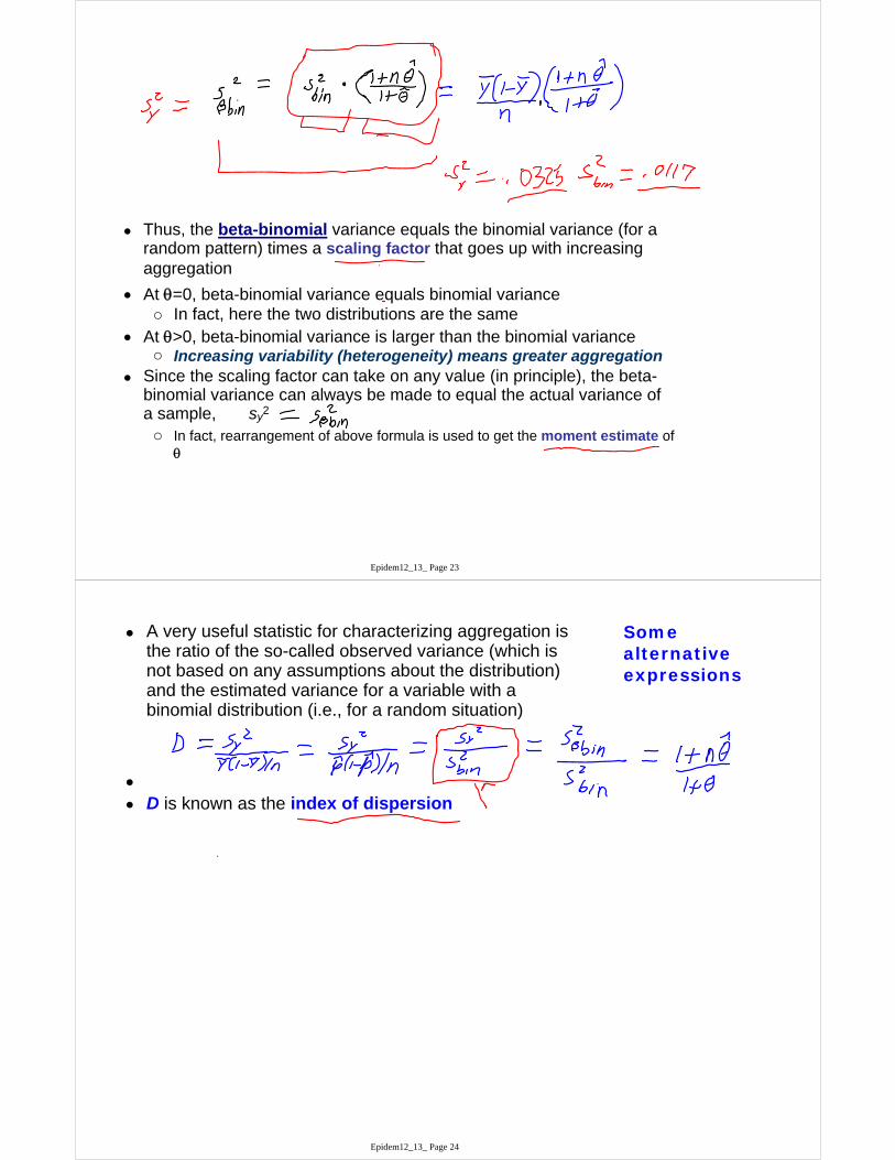
Thus, the beta-binomial variance equals the binomial variance (for a random pattern) times a scaling factor that goes up with increasing aggregation

At =0, beta-binomial variance equals binomial variance○ In fact, here the two distributions are the same

At >0, beta-binomial variance is larger than the binomial variance○ Increasing variability (heterogeneity) means greater aggregation

Since the scaling factor can take on any value (in principle), the beta-binomial variance can always be made to equal the actual variance of a sample, sy

2

○ In fact, rearrangement of above formula is used to get the moment estimate of


A very useful statistic for characterizing aggregation is the ratio of the so-called observed variance (which is not based on any assumptions about the distribution) and the estimated variance for a variable with a binomial distribution (i.e., for a random situation)

D is known as the index of dispersion

Some alternative expressions


Very simple evaluation of aggregation:○ Get D (from observed variance and binomial

variance) D=1: random D>1: aggregated D<1: regular (uniform)

□ Minimum D is 0○ Test of aggregation:

(N-1)D□ Has chi-square distribution with N-1

df if random (i.e., if binomial)

□ Null hypothesis: random (binomial)□ If (N-1)D > critical chi-square, then

conclude aggregated


12345678910111213141516171819202122232425262728293031323334353637383940414243444546474849505152535455565758590

3

6

9

12

15

0 1 2 3 4 5 6 7 8 9 10 11 12 13


0

4

8

12

16

Fre

quen

cy

Obs.

Bin.

BBD


Meaning of aggregation based on variances and/or discrete distributions

The beta-binomial is not the only distribution that can describe aggregated disease incidence data, but is the most common○ It has very useful theoretical properties (not discussed here)○ A special case (=0) is the binomial (random)

Distributions of this type explicitly characterize heterogeneity of the random variable

○ When the variable is overdispersed (so that is a measure of overdispersion or degree of heterogeneity)

The beta-binomial (or similar distribution) characterizes the pattern of disease at the spatial scale of the sampling unit or smaller○ That is, represents aggregation of diseased individuals within

sampling units, not across sampling units. SMALL-SCALE PATTERNS (e.g., small patches of disease)

○ If the data were mapped (not required, because all this works for sparse-sampling data collection), one would not necessarily see big patches of high disease and gaps of low (no) disease)

Greater aggregation within sampling units is manifested by greater variability between sampling units!


Meaning of aggregation based on variances and/or discrete distributions (continued)

Small scale pattern can be made clear by considering the

intra-cluster correlation ()○ The correlation of disease status of individuals within a

sampling unit (an average, of sorts, across all sampling units)

○ Tendency for individuals within a sampling unit to have the same value

It can be shown that: = /(1+)

○ = 0: no correlation (no aggregation)○ > 0: aggregation (maximum of 1)

Can also be derived with no consideration of the statistical distribution


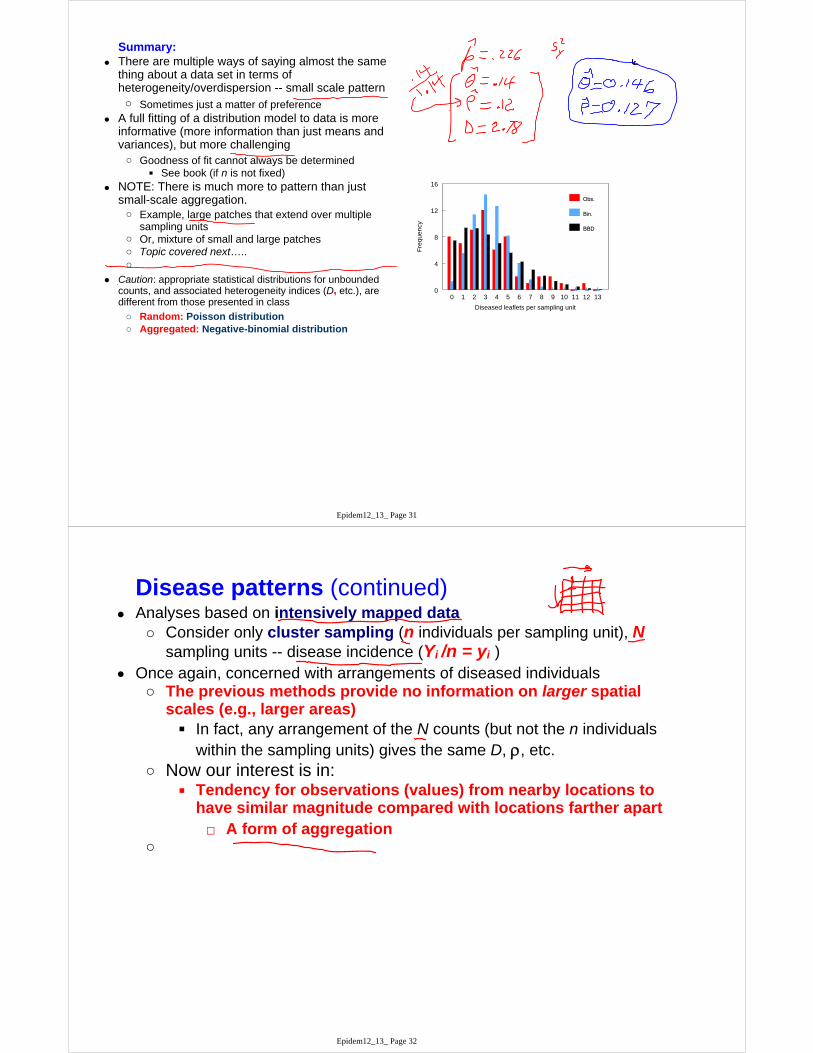
Summary: There are multiple ways of saying almost the same

thing about a data set in terms of heterogeneity/overdispersion -- small scale pattern○ Sometimes just a matter of preference

A full fitting of a distribution model to data is more informative (more information than just means and variances), but more challenging○ Goodness of fit cannot always be determined

See book (if n is not fixed) NOTE: There is much more to pattern than just

small-scale aggregation.○ Example, large patches that extend over multiple

sampling units○ Or, mixture of small and large patches○ Topic covered next…..○

Caution: appropriate statistical distributions for unbounded counts, and associated heterogeneity indices (D, etc.), are different from those presented in class

○ Random: Poisson distribution○ Aggregated: Negative-binomial distribution

0 1 2 3 4 5 6 7 8 9 10 11 12 13


0

4

8

12

16

Fre

quen

cy

Obs.

Bin.

BBD


Disease patterns (continued) Analyses based on intensively mapped data

○ Consider only cluster sampling (n individuals per sampling unit), Nsampling units -- disease incidence (Yi /n = yi )

Once again, concerned with arrangements of diseased individuals○ The previous methods provide no information on larger spatial

scales (e.g., larger areas) In fact, any arrangement of the N counts (but not the n individuals

within the sampling units) gives the same D, , etc.○ Now our interest is in:

Tendency for observations (values) from nearby locations to have similar magnitude compared with locations farther apart□ A form of aggregation

○



For the typical analyses here, Y (or y) can be either a discrete (count; not just binary) or continuous random variable○ Disease incidence, density, or severity○ Key: spatial referencing of the sampling units

Intensive mapping

Three (general) major methods:○ Spatial autocorrelation analysis○ Semivariogram analysis (mirror image of autocorrelation)

Geostatistics○ SADIE (counts only -- with or without natural denominator)

Joe Perry et al. (Rothamsted) Turechek, Madden, Xiangming Xu (see book)

Of course, there are other analyses for sampling units consisting of single individuals

Important reminder: methods unique to intensely mapped data (spatial referencing) cannot be applied to sparse sampling (i.e., if the spatial locations are not known, one cannot use methods that require the spatial locations!)○ But methods of sparse sampling can be applied to intensely

mapped data, if Y is discrete (although these would not take advantage of the spatial referencing)


Spatial autocorrelation:○ The degree of association in Y (or y)

between neighboring sampling units○ For immediate neighbors (each sampling unit

with those next to it), r(1) Most commonly determined

○ For the next most immediate neighbors, r(2) And so on

○ The larger the r(), the more aggregated


Methodology comes from time series analysis


Spatial autocorrelation

Magnitude of r(1) is evaluated.○ Large values indicate aggregation, at a spatial

scale larger than the size of the sampling unit. Standard error of r(1): (1/N1)1/2

Note: The analyses here are for a different scale than the heterogeneity analyses (beta-binomial, D, etc.) presented earlier.

Thus, the methods can give different results, since they are not characterizing the same thing.


ACF of C260

-1.0 -0.8 -0.6 -0.4 -0.2 0.0 0.2 0.4 0.6 0.8 1.0

+----+----+----+----+----+----+----+----+----+----+

1 -0.020 XX

2 -0.087 XXX

3 0.251 XXXXXXX

4 0.148 XXXXX

5 0.149 XXXXX

6 0.080 XXX

7 0.035 XX

8 0.053 XX

9 0.196 XXXXXX

10 0.142 XXXXX

11 -0.206 XXXXXX

12 0.111 XXXX

13 0.045 XX

Spatial autocorrelationsStrawberry Phomopsis data (again)

1 2 3 4 5 6 7 8 9 10 11 12 13 14 15 16 17 18 19 20 21 22 23 24 25 26 27 28 29 30 31 32 33 34 35 36 37 38 39 40 41 42 43 44 45 46 47 48 49 50 51 52 53 54 55 56 57 58 590

3

6

9

12

15


Synthesis There are many ways of characterizing spatial patterns of organisms,

including diseased individuals Some approaches are dependent on type of random variable (for discrete

data only)! -- the nature of Y○ Generally: Appropriate methods for characterizing small-scale patterns (with

sparse sampling or intensive mapping)

Some approaches depend on intensive mapping (spatially referenced sampling units) -- the nature of the sampling method○ Appropriate methods for characterizing larger scale patterns

Can be for a wider range of disease variables

Reminder: we only discussed methods for sparse sampling and intensive mapping when there is a count (Y out of n) in each sampling unit

Unless a pattern is truly random, there is a scale to the pattern○ That is, there may be small clumps (not even visible (in a sense) from a

map, but quantifiable using discrete-data analyses○ There may be large and very large clumps (patches) dispersed over the

area of interest, quantifiable through autocorrelations, etc. Results of different classes of analyses may be complementary, not

contradictory In general, when intensive maps are available, one should

always assess small scale and larger scale patterns



Clarification: by discrete here, I mean counts of individuals out of n in each sampling unit --other distributional approaches are used when there is not a natural denominator (but still discrete)--see textbook.


Reading assignment:Sections 9.1 - 9.3 in Chapter 9 (pages 235-238)

For background (optional):

Sections 9.4 and 9.9


Spatial analysis of epidemics: Disease patterns - CFAES analysis of epidemics: Disease patterns...

Documents

Transcript of Spatial analysis of epidemics: Disease patterns - CFAES analysis of epidemics: Disease patterns...