Simulation Tools for

Hybrid Electric Vehicle Architecture Simulations

Undergraduate Honors Thesis

Presented in Partial Fulfillment of the Requirements for

Graduation with Distinction at

The Ohio State University

By

Arjun Khanna

* * * * *

The Ohio State University

2014

Defense Committee:

Dr. Giorgio Rizzoni

Dr. Shawn Midlam-Mohler

Copyrighted by

Arjun Khanna

2014

ii

ABSTRACT

Increasingly stringent regulations on emissions require automobile manufacturers to

find new ways to reduce the emissions produced by their vehicles. If current trends provide

for an indication of where the automotive industry is headed, hybrid electric vehicles

(HEVs) and electric vehicles (EVs) will become very prevalent in the market in coming

years. These technologies are all relatively new and still need much development before

they can hold a significant place in the automotive market. It is for this reason that

companies are investing heavily in training the next generation of engineers to work on

this problem. EcoCAR 3, a four year long Advanced Vehicle Technology Competition

(AVTC), is one way companies are pursuing this.

EcoCAR 3 challenges the engineering students to modify a stock Chevrolet

Camaro, donated by GM, to reduce the vehicle’s energy consumption and tailpipe

emissions, while maintaining standard vehicle performance. Due to the presence of

multiple components in a HEV (engine, battery-pack and at least one electric machine), the

complexity of optimizing the operation of the vehicle’s powertrain components

significantly increases in comparison to a conventional vehicle. One of the topics that

EcoCAR 3 series stresses during year 1 is architecture selection for the Chevrolet Camaro,

which involves the team to select a vehicle architecture that meets the goals of both the

competition and the team. Increasing demand for HEV designs require automated

1

modeling and simulation tools to construct a design space search. Composability and

scalability are highly desirable in these simulators to provide design candidates.

The work described in this project focuses towards the tools developed and the

validation done for these tools. These tools were developed for the EcoCAR 3 team of the

Ohio State Universiy, which would provide assistance in generating different size engine

fuel consumption maps and different size electric machine efficiency maps quickly. The

maps generated by these tools can then be utilized to test how varying engine and electric

machine sizes can affect the overall performance of the vehicle with different architectures.

2

ACKNOWLEDGMENTS

I would like to thank Dr. Giorgio Rizzoni for the chance to participate in this

undergraduate research project. I would especially like to thank Dr. Shawn Midlam-

Mohler, for all the guidance he has given me during this research project. I would like to

thank the entire EcoCAR team, especially Katherine Bovee and Matt Yard for introducing

me and helping me learn about Hybrid Electric Vehicles.

3

TABLE OF CONTENTS

Page

ABSTRACT ........................................................................................................................ 1

ACKNOWLEDGMENTS .................................................................................................. 3

TABLE OF CONTENTS .................................................................................................... 3

LIST OF FIGURES ............................................................................................................ 6

LIST OF TABLES ............................................................................................................ 11

Chapter 1: Introduction ....................................................................................................... 1

1.1 Motivation ........................................................................................................... 1 1.2 EcoCAR 3 ........................................................................................................... 2 1.3 Project Objective ................................................................................................. 3

Chapter 2: Literature Review .............................................................................................. 4

2.1 Hybrid Electric Vehicle ...................................................................................... 4 2.2 HEV Architectures .............................................................................................. 7 2.2.1 Series ............................................................................................................... 7 2.2.2 Parallel ............................................................................................................ 9 2.2.3 Multi-mode (Power Split) ............................................................................. 12

2.3 Energy Converters ............................................................................................ 14 2.3.1 Internal Combustion Engines ........................................................................ 15 2.3.2 Electric Machines.......................................................................................... 20

2.4 Scalable Approach to HEV modeling ............................................................... 26 2.4.1 Scaling Methods............................................................................................ 27

2.4.1.1 Engine Fuel Consumption and Efficiency Maps .................................. 30 2.4.1.2 Willans Line Model for Engines ........................................................... 32 2.4.1.3 Electric Machine Efficiency Map ......................................................... 35 2.4.1.4 Willans Line Model for Electric Machines ........................................... 37

2.5 EcoSIM ............................................................................................................. 39 2.5.1 Overview ....................................................................................................... 40

Chapter 3: Scaling Methods .............................................................................................. 42

3.1 Introduction ....................................................................................................... 42 3.2 Engine Scaling .................................................................................................. 42 3.3 Electric Machine Scaling .................................................................................. 53

4

Chapter 4: Scaling validation ............................................................................................ 61

4.1 Introduction ....................................................................................................... 61 4.2 Engine Scaling .................................................................................................. 61 4.2.1 Actual vs. Actual Engines’ Comparison ....................................................... 62 4.2.2 Actual vs. Predicted Engines’ Comparison .................................................. 67

4.3 Electric Machine Scaling .................................................................................. 75 4.3.1 Actual vs. Predicted EM Comparison ........................................................... 76

Chapter 5: Conclusion And Future Work ......................................................................... 81

Chapter 6: Bibliography .................................................................................................... 82

5

LIST OF FIGURES

Figure Page

Figure 1: Major Components of a Hybrid Electric Vehicle ................................................ 6

Figure 2: Plug-in Series Hybrid Electric Vehicle [9].......................................................... 8

Figure 3: Plug-in Parallel Hybrid Electric Vehicle Architecture [9] ................................ 10

Figure 4: Commonly used Mechanical Torque Couplings [9] ......................................... 10

Figure 5: Series-Parallel Hybrid Architecture using a Planetary Gear Unit [9] ............... 12

Figure 6: HEV Sales in the United States [10] ................................................................. 13

Figure 7: Illustration of Power Flow in a HEV [9] ........................................................... 14

Figure 8: Fuel Consumption at 2000 rpm [14] ................................................................. 18

Figure 9: Comparison of Naturally Aspirated and Turbocharged Downsized Engines

(a)Power (HP) (b) Torque (lb-ft) [14] ....................................................................... 19

Figure 10: Industrial and Traction Motors’ Cross-Section (a) DC Motor (b) IM (c) PM

Brushless Motor (d) SRM [15] ................................................................................. 21

Figure 11: Typical Motor Torque vs. Speed Characteristic [15] ...................................... 22

Figure 12: Typical Switched Reluctance Motor Torque vs. Speed Characteristic [15] ... 23

6

Figure 13: Typical Induction Motor Torque vs. Speed Characteristic [15] ...................... 24

Figure 14: Typical Permanent Magnet Brushless Motor Torque vs. Speed Characteristic

[15] ............................................................................................................................ 25

Figure 15: Input-Output Relationship of an Energy Converter [11]................................. 29

Figure 16: Fuel Consumption Map of a 1.9 L Turbocharged Diesel Engine ................... 30

Figure 17: Efficiency Map of a 1.9 L Turbocharged Diesel Engine ................................ 31

Figure 18: Geometry of Cylinder, Piston, Connecting Rod and Crankshaft in an Engine

[12] ............................................................................................................................ 33

Figure 19: PM Brushless Motor with a 1.4 L Rotor Efficiency Map ............................... 36

Figure 20: Rotor Physical Parameters............................................................................... 38

Figure 21: EcoSIM Top Level Structure .......................................................................... 40

Figure 22: Fuel Consumption Map of a 1.6 L NA-SI Engine .......................................... 44

Figure 23: Power Output Map of a 1.6 L NA-SI Engine .................................................. 44

Figure 24: Efficiency Map of a 1.6 L NA-SI Engine ....................................................... 45

Figure 25: Normalized Efficiency Map of a NA-SI Engine ............................................. 47

Figure 26: Predicted Efficiency Map of a 1.8L NA-SI Engine ........................................ 48

7

Figure 27: Predicted Power Map of a 1.8L NA-SI Engine ............................................... 49

Figure 28: Predicted Fuel Consumption Map of a 1.8L NA-SI Engine ........................... 50

Figure 29: Actual 1.6 L and Predicted 1.8 L engine (a-b) Fuel consumption, (c-d)

Efficiency and (e-f) Power Output comparison ........................................................ 51

Figure 30: Energy Conversion Efficiency for Existing Brushless PM Motor .................. 55

Figure 31: Power Map for Existing Brushless PM Motor ................................................ 55

Figure 32: Normalized Efficiency Map of a Brushless PM Motor ................................... 56

Figure 33: Predicted energy conversion efficiency map for brushless PM motor ............ 57

Figure 34: Predicted Power Map for Brushless PM Motor .............................................. 58

Figure 35: Actual 1.4 L and Predicted 2.1 L Rotor Volume EM’s (a-b) Energy Conversion

Efficiency, (c-d) Power Map Comparison ................................................................ 60

Figure 36: Engine Comparisons........................................................................................ 62

Figure 37: Actual Engines (1&2) (a&b) Fuel Consumption and (c&d) Efficiency

Comparison ............................................................................................................... 63

Figure 38: Maximum Torque-Speed Curves of 1.8 L NA-SI Engines (1&2) .................. 64

Figure 39: 1.8 L Engine (1) vs. 1.8 L Engine(2) Fuel Consumption Comparison (a)

Histogram, (b) Contour ............................................................................................. 66

8

Figure 40: 1.8 L Engine (1) vs. 1.8 L Engine(2) Efficiency Comparison (a) Histogram, (b)

Contour ..................................................................................................................... 66

Figure 41: Actual vs. Predicted Engine’s (a&b) Fuel Consumption and (c&d) Efficiency

Comparison ............................................................................................................... 68

Figure 42: Maximum Torque-Speed Curves Comparison of Actual vs. Predicted 1.8 L NA-

SI Engines ................................................................................................................. 70

Figure 43: Actual (1) vs. Predicted 1.8 L Engine Fuel Consumption Error (a) Histogram,

(b) Contour ................................................................................................................ 72

Figure 44: Actual (1) vs. Predicted 1.8 L Engine Efficiency Error (a) Histogram, (b)

Contour ..................................................................................................................... 72

Figure 45: Predicted vs. Actual (a&c) and Actual vs. Actual (b&d) Efficiency and Fuel

Consumption Error Histograms ................................................................................ 74

Figure 46: Electric Machine Comparisons ....................................................................... 75

Figure 47: Actual (a) vs. Predicted (b) EM’s Energy Conversion Efficiency Comparison

................................................................................................................................... 77

Figure 48: Maximum Torque-Speed Curves Comparison of Actual vs. Predicted EMs with

2.1 L Rotors .............................................................................................................. 78

9

Figure 49: Actual vs. Predicted EMs with 2.1 L EMs’ Fuel Efficiency Error (a) Histogram,

(b) Contour ................................................................................................................ 79

10

LIST OF TABLES

Table Page

Table 1: Specifications for the Existing Engine ............................................................... 43

Table 2: Specifications for the Predicted Engine .............................................................. 47

Table 3: Original vs. Scaled Engine Parameters Comparison .......................................... 52

Table 4: Specifications for the Existing EM ..................................................................... 54

Table 5: Specifications of the Predicted EM .................................................................... 57

Table 6: Original vs. Scaled EMs’ Parameters Comparison ............................................. 60

Table 7: Actual 1.8 L NA-SI Engines’ Parameters Comparison ...................................... 63

Table 8: 1.8 L Engine (1) and 1.8 L Engine (2) Error Statistics ....................................... 67

Table 9: Actual vs. Predicted 1.8 L NA-SI Engines’ Parameter Comparison .................. 68

Table 10: Actual 1.8 L Engine (1) and Predicted 1.8 L Engine Error Statistics ............... 72

Table 11: Actual vs. Actual and Predicted vs Actual Efficiency and Fuel Consumption

Error Statics .............................................................................................................. 74

Table 12: Actual vs. Predicted PM Motors with 2.1 L Rotors’ Parameter Comparison .. 77

Table 13: Actual and Predicted EMs with 2.1 L Rotor Efficiency Error Statistics .......... 79

11

CHAPTER 1: INTRODUCTION

1.1 Motivation

Today, the increasing number of vehicles worldwide is causing a significant

negative impact on air quality and human health [1]. Emissions standards set by the U.S.

Environmental Protection Agency (EPA) are getting more stringent in addition to the rising

petroleum prices [2]. Because of all these factors, the rate of vehicle technology change in

the automotive industry is increasing and moving towards a low-carbon future [3], meaning

less emissions pertaining to carbon monoxide (CO), nitrogen oxides (NOx) and greenhouse

gases (GHG).

If current trends provide for an indication of where the automotive industry is headed,

hybrid electric vehicles (HEVs) and electric vehicles (EVs) will become very prevalent in

the market in the coming years [3]. HEVs consist of powertrains that combine more than

one form of energy. For example, the Chevrolet Volt is an HEV that combines a

conventional gasoline powered engine with electrical power generation provided from a

battery pack. EVs consist of a powertrain powered solely by electricity, usually coming

from a battery pack.

These technologies are all relatively new and still need much development before

they can hold a significant place in the automotive market. It is for this reason that

companies are investing heavily in training the next generation of engineers to work on

this problem. EcoCAR 3, an Advanced Vehicle Technology Competition (AVTC), is one

1

way companies are pursuing this.

1.2 EcoCAR 3

The Ohio State University is taking part in a four year long Advanced Vehicle

Technology Competition (AVTC), EcoCAR 3. This competition is headline sponsored by

The U.S. Department of Energy and General Motors (GM) the competition is managed by

Argonne National Laboratory. The purpose of this competition is for collegiate student

teams to reduce the environmental impact of a vehicle by minimizing fuel consumption

and reducing its emissions, while maintaining the vehicle’s original performance and

consumer acceptability. The team will be provided with a stock Chevrolet Camaro, donated

by GM. Each team’s task will be to design, build, and optimize a new powertrain for their

vehicle, resulting in a fully functioning prototype vehicle by the end of the fourth year. The

prototype vehicles created by each team will be evaluated over a wide range of metrics that

include the vehicle’s fuel economy, its emissions, drivability, acceleration, consumer

acceptability, and braking.

The competition is broken up into four years and there is a final competition at the

end of each year. The EcoCAR 3 competition started in the fall of 2014 and is currently in

its first year. In the first year of the EcoCAR 3 competition series stresses the application

of the Vehicle Development Process, math-based modeling tools, architecture selection,

communications, and project management.

2

1.3 Project Objective

One of the topics that EcoCAR 3 series stresses on during year 1 is the architecture

selection for the Chevrolet Camaro, which involves the team to select a vehicle architecture

that meets the goals of both the competition and the team. To select the best architecture

the team needs to have a solid understanding of the strengths and weaknesses of various

powertrains. To understand these strengths and weaknesses, team needs to evaluate

multiple powertrain components and subsystems as part of a total vehicle system, and

finally choose or reject the specific components (e.g., engines, motors, batteries,

transmissions, subsystems) for their proposed vehicle.

The entire process of evaluating each component that best fits the needs for the

team and competition is tedious. This project develops tools for the EcoCAR 3 team, which

would provide assistance in generating different size engine fuel consumption maps and

different size electric machine efficiency maps quickly. The maps generated by these tools

can then be utilized to test how varying engine and electric machine sizes can affect the

overall performance of the vehicle. This would allow the EcoCAR 3 team to make an

informed decision on what size engine and electric machine could be used in different

architectures. This would eventually help the team select the architecture that best fits the

competition and the consumer needs which eventually gives the team a direction for the

rest of the competition.

3

CHAPTER 2: LITERATURE REVIEW

2.1 Hybrid Electric Vehicle

There has been much research and advancement in recent years in the area of

electrification of vehicles. The three major kinds of electrified vehicles that are being

commercially produced are Electric Vehicles (EV), Hybrid Electric Vehicles (HEV) and

Plug-in Hybrid Electric Vehicle (PHEV) [4]. Each of the three kinds of electrified vehicle

have their respective components and their pros and cons, which are discussed in this

section.

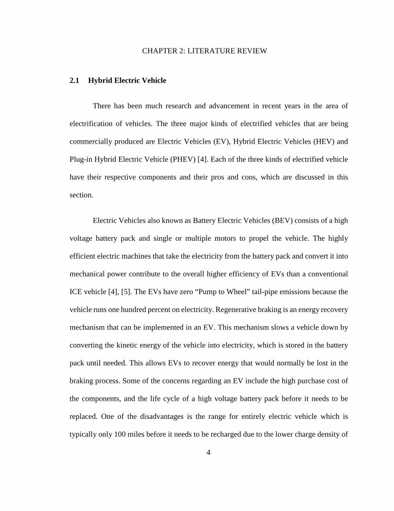
Electric Vehicles also known as Battery Electric Vehicles (BEV) consists of a high

voltage battery pack and single or multiple motors to propel the vehicle. The highly

efficient electric machines that take the electricity from the battery pack and convert it into

mechanical power contribute to the overall higher efficiency of EVs than a conventional

ICE vehicle [4], [5]. The EVs have zero “Pump to Wheel” tail-pipe emissions because the

vehicle runs one hundred percent on electricity. Regenerative braking is an energy recovery

mechanism that can be implemented in an EV. This mechanism slows a vehicle down by

converting the kinetic energy of the vehicle into electricity, which is stored in the battery

pack until needed. This allows EVs to recover energy that would normally be lost in the

braking process. Some of the concerns regarding an EV include the high purchase cost of

the components, and the life cycle of a high voltage battery pack before it needs to be

replaced. One of the disadvantages is the range for entirely electric vehicle which is

typically only 100 miles before it needs to be recharged due to the lower charge density of

4

the battery [4]. The issue of charging also brings up the issue of city infrastructure. To

allow for an EV to travel long distances, city infrastructure all over the nation needs to

change to include charging stations to make it possible for electric vehicle to recharge its

batteries just like conventional cars re-fuel today. Despite the disadvantages, the

advancement of technology in the future could make the use of electric vehicles a viable

and a beneficial choice for the everyday consumer and the environment.

Hybrid electric vehicles (HEVs) were developed to overcome the limitations of ICE

vehicles and EVs [6]. HEVs are a subset of hybrid vehicles, which utilizes both the liquid

fuel (gasoline, diesel, E85 etc.) as well as electricity to provide power to the wheels. Some

of the major components that go into the making of an HEV power-train are: internal

combustion engine, a battery pack and at least one electric machine [4]. The previously

mentioned components are also illustrated in Figure 1. Having two propulsion systems

within the same vehicle provides some advantages to HEVs over a conventional vehicle.

One of the advantages in a HEV is that a downsized engine can be used with the high

voltage battery pack and a motor to propel the vehicle. This provides a HEV the ability to

have high performance while providing better fuel economy and reduced emissions. Due

to the internal combustion engine in HEVs, it allows the vehicle to have the same travelling

range as a conventional vehicle [4]. Just like EVs the HEVs get to utilize the regenerative

braking. Although there are a lot of advantages of using a HEV, there are some

shortcomings as well. One of the major drawbacks of HEVs currently is the purchase price

for consumers due to the added components making them out of reach for consumers even

though HEVs provide better fuel economy. Another disadvantage of HEVs over EVs is the

5

lack of all-electric mode in the vehicle. The option of a Plug-in Hybrid Electric Vehicle

(PHEV) can solve the problem of all electric range of a HEV.

Figure 1: Major Components of a Hybrid Electric Vehicle

A Plug-in Hybrid Electric Vehicle has been defined by SAE [7] as: “A hybrid

vehicle with the ability to store and use off-board electrical energy in the RESS

(rechargeable energy storage system).” These systems are in effect an incremental

improvement over the HEV with the addition of a large battery with greater energy storage

capability, a charger, and modified controls for battery energy management and utilization.

The better fuel economy, longer travelling range and better performance are some of the

positive elements concerning PHEVs which can run on 100% electric mode for short

distances. Like both the EVs and HEVs, PHEVs also have a high purchase price [8].

Various combinations of architectures and sizes of components can influence the

performance attributes of an HEV significantly. Some of the major HEV components,

Electric Machine

Major Components of a Hybrid Electric Vehicle

IC Engine Transmission Battery Pack

6

architectures and techniques used to scale the internal combustion engines and electric

machines are described in the following sections.

2.2 HEV Architectures

The energy flow through the components of a Hybrid Electric Vehicle can be

arranged and configured in various ways that define the architecture of the vehicle. This

section of the thesis reviews the different possible HEV architectures, their respective

operating modes, and their pros and cons.

2.2.1 Series

In series HEV architecture, an engine is coupled with an electric machine, which

works as a generator to convert the energy produced by the engine into electricity which is

used to charge the battery pack. The battery provides power to a second electric machine

that converts the electricity to mechanical power which in turn propels the vehicle [9].

Figure 2 shows a model of plug-in series hybrid electric drivetrain. There are six possible

different operation modes in a plug-in series HEV:

1) Battery alone mode: engine is off and the vehicle is powered by the battery only;

2) Engine alone mode: power from ICE only;

3) Combined mode: both ICE set and battery provides power to the traction motor;

4) Power split mode: ICE/G power split to drive the vehicle and charge the battery;

7

5) Stationary charging mode;

6) Regenerative braking mode [5].

Figure 2: Plug-in Series Hybrid Electric Vehicle [9]

Decoupling engine from the wheels provide some advantages to the series HEV

architecture. The first advantage being that the flexibility to place the ICE anywhere in the

car [6]. Also, because the engine is not directly connected to the wheels in the series HEV,

the vehicle has the option to run the internal combustion engine in its optimal operating

range the entire time which allows the HEV to have a greater engine efficiency. A multi-

gear transmission in this architecture is unnecessary because of favorable torque-speed

characteristics of the electric motor. The controls and packaging are simpler because of the

8

simpler drive train. Only electrical cables connect the batteries, the generator and the

traction motor.

In addition to the advantages of a series HEV architecture, there are some

disadvantages as well. Perhaps the greatest disadvantage is the lower efficiency of the

series hybrid electric vehicle outside of its optimal range. The lower efficiency is caused

by the need for three propulsion devices: the ICE, the generator, and the electric motor.

Similar to EVs, extra precautions come in to play when the vehicle needs to make lengthy

trips versus short commutes to work or the supermarket. The series HEV will need to have

the traction motor sized to provide maximum sustained power since it is the only traction

source, which will make the overall vehicle’s price go up. For shorter trips this would not

be the case but for the vehicle to travel long distances the consumer may have a high out

of pocket cost [6]. Additionally the series HEV is disadvantaged because it requires two

electric machines which means twice the energy conversions causing twice the energy loss.

Also the additional motor means more additional weight of the vehicle which affects the

overall performance, fuel consumptions and emissions of the vehicle [9].

2.2.2 Parallel

Both the engine and the electric machine are capable of propelling the vehicle at

the same time in a parallel HEV architecture. As shown in Figure 3, a plug-in parallel

hybrid architecture consists of a battery, an engine and an electric machine. The electric

machine and the engine are mechanically coupled together. The mechanical coupling could

be one of the following: a gearbox, a pulley-belt unit or a sprocket chain unit or even a

9

single axle [9]. Figure 4 shows the schematics of previously mentioned possible

mechanical couplings in a parallel hybrid electric drive train.

Figure 3: Plug-in Parallel Hybrid Electric Vehicle Architecture [9]

Figure 4: Commonly used Mechanical Torque Couplings [9]

The following are the possible different operation modes of parallel hybrid:

10

1) Motor alone mode: engine is off, vehicle is powered by the motor only;

2) Engine alone mode: vehicle is propelled by the engine only;

3) Combined mode: both ICE and motor provides power to the drive the vehicle;

4) Power split mode: ICE power is split to drive the vehicle and charge the battery (motor

becomes generator);

5) Stationary charging mode;

6) Regenerative braking mode (include hybrid braking mode) [5].

One advantage of the parallel HEV architecture is that it is more efficient than the

series architecture because it only requires the internal combustion engine and the electric

machine, both of which are directly connected to the wheels. This results in decreased

energy loss [4]. Another advantage of the parallel architecture is the compact size due to

the reduced number of components as compared to a series HEV [6]. Also, a generator is

usually not needed with this configuration and a smaller traction motor can be used [9].

While there are advantages there are a few disadvantages as well. The structure and

control of parallel vehicles is complex and due to the mechanical coupling between the

driven wheels and the engine, it is difficult for the vehicle to perform in a narrow optimal

region in comparison to series HEV [9]. Since the optimal region is not often achievable

these vehicles will often employ the use of a clutch for operation [6].

11

2.2.3 Multi-mode (Power Split)

A multi-mode hybrid vehicle encompasses the features of both the parallel and the

series HEV architectures. One ICE and two electric machines in conjunction with different

configurations of planetary gear-set or clutches gives the vehicle the extra degree of

freedom of switching modes between series and parallel modes.

Figure 5: Series-Parallel Hybrid Architecture using a Planetary Gear Unit [9]

Figure 5 explains an example of Toyota Prius’ series-parallel architecture. This

particular series-parallel hybrid architecture consists of an engine, a generator/motor, a

traction motor and a planetary gearbox. Series mode is achieved by using the planetary

gear to decouple the engine speed from the wheel speed. The decoupling of the engine from

the wheels is done by adjusting the speed of the generator/motor, thus allowing the engine

to operate at its most efficient operating points at all times. Additionally, the architecture

12

is able to operate in a parallel mode by locking the stator and rotor of the generator/motor

together and de-energizing it. When stator and rotor of the generator/motor are locked in

place, the planetary gear unit becomes a simple gearbox with a single fixed gear ratio, thus

allowing the vehicle to operate in parallel mode [9].

The multi-mode configuration combines the best qualities of both series and parallel

architectures so that the vehicle will be operating efficiently and deliver high performance

[4]. Figure 6 from the United States Department of Energy and the Alternative Fuels Data

Center, outlines the overall sales of HEV’s in the U.S. market. From Figure 6, it is clear

that the Toyota Prius has a commanding market share for HEVs in the United States. What

sets the Prius apart from the competition is its advanced vehicle architecture, which is a

multi-mode as expressed in Figure 5. The multi-mode HEV architecture is proven to be

dominant, so it is a safe assumption to make that a multi-mode HEV is a good balance

between cost, complexity, and performance.

Figure 6: HEV Sales in the United States [10]

13

2.3 Energy Converters

Energy converters are the components in a HEV that are responsible for energy

conversions between energy domains (chemical to mechanical, electrical to mechanical

etc.) [11]. As represented in Figure 7 and mentioned before HEV’s consist of two

powertrains and hence two energy converters: engine and electric machine.

Figure 7: Illustration of Power Flow in a HEV [9]

This section introduces different types of the energy converters, their different

performance characteristics due to the differences in the technologies and also mentions

the advantages and disadvantages pertaining to the different types of energy converters.

This section of the thesis stresses on different technologies and performance aspects

because the tools developed for this project are sensitive to these differences.

14

2.3.1 Internal Combustion Engines

An internal combustion engine is an energy converter that transforms

chemical energy into mechanical energy with a certain efficiency. In an Internal

combustion engines (ICEs), as opposed to external combustion engines, the energy

source is a combustible mixture, and the combustion products is the working fluid. In

external combustion engines, the combustion products is used to heat a second fluid that

acts as the working fluid [12]. There are many different types of ICEs and performance

of these different types of ICE depends majorly on the fuel type used by the engine

(Gasoline, E85, Diesel, etc.), technology used by the engine (turbo/super-charged,

GDI, etc.) and the overall size of the engine.

Gasoline engines, approximated by an Otto engines, mix the air and the fuel in

the intake system prior to the entry of the engine cylinders using either a carburetor

or a fuel injection system. In a diesel engine, the air alone enters the cylinder; without

getting mixed with the diesel fuel. The diesel fuel is injected directly into the engine

cylinder just before the combustion process is required to start. In the case of spark ignition

(SI) engines, the compression ratio of the cylinder is in the range of 9 to 13 and is limited

by octane rating of the fuel. In compression ignition (CI) (diesel) engines, the compression

ratio for air is 12 to 24. The high compression ratio of air creates high temperatures which

ensures the diesel fuel can self-ignite [12]. In the case of CI engines, the value of

compression ratio is higher; according to Equation (2.1) CI engines have the potential to

achieve higher fuel conversion efficiency while in the case of SI engines the lower

15

compression ratio reduces their potential to achieve higher efficiency [12]. Dedicated E85

engines, like CI engines benefit from a higher compression ratio as well, increasing their

potential to achieve a higher efficiency. This is because E85 has a relatively high octane

number making it more tolerant of high compression ratios.

1

11fcr γη−

= − (2.1)

Performance of an ICE also depends on the technology used in the engine: naturally

aspirated (admitting atmospheric air), supercharged (admitting pre-compressed fresh

mixture), and turbocharged (admitting fresh mixture compressed in a compressor driven

by an exhaust turbine). These technologies have their respective pros and cons which are

further described in this section.

A supercharger is an air compressor that increases the pressure or density of air

supplied to an ICE, in turn increasing the volumetric efficiency of the engine [12]. Defines

volumetric efficiency as the parameter, which is used to measure the effectiveness of an

engines induction process. Power for the supercharger in an ICE is usually provided by

mechanically coupling the engine's crankshaft to the supercharger by means of a belt, gear,

shaft, or chain. A supercharged engine provides excellent low-end torque capabilities and

very good response [13]. However, there are some drawbacks associated with

supercharging an engine. Due to the mechanical coupling, the engine has to burn extra fuel

to provide power to drive the supercharger. The parasitic losses of a supercharger can

negate some of the fuel savings of downsizing an engine. Even though, the parasitic losses

16

of the supercharger can be quite significant at high engine speeds, the indicated mean

effective pressure (IMEP) is higher than the IMEP for a naturally aspirated (NA) or

turbocharged (TC) engine with the same power output [13].

When power in a supercharger is provided by a turbine powered by exhaust gas of

the engine, a supercharger is known as a turbocharger. Turbo charging counteracts the

power lost from downsizing without the parasitic losses associated with supercharging. A

turbocharged engine also runs at significantly higher BMEP levels than a naturally

aspirated engine. The upper limit of BMEP levels that can be expected from a naturally

aspirated engine is ~ 13.5 bar, whereas a turbocharged engine can produce BMEP levels

in excess of 20 bar [14]. By using a small displacement engine with a turbocharger, the

smaller engine works harder (higher in cylinder load) which results in lower pumping

losses as the throttle has to be further open [14]. Boosting an engine via turbocharger has

its own deficits. Turbocharged systems typically have a delay in response as compared to

a supercharged system or naturally aspirated systems [13]. The back pressure increase

associated with turbocharging results in an increase in pumping losses and the need to run

with lower overlap at higher speed to avoid insufficient exhaust gas scavenging. The turbo

also acts as a heat sink, which can slow the catalyst heating and catalyst light-off after start,

thus hurting emission reduction strategies [13]. Turbo charger manufacturers are aware of

these issues and designs are being validated that address these concerns. A comparison

between boosted engines and naturally aspirated engine done by [14] is used to highlight

these differences.

17

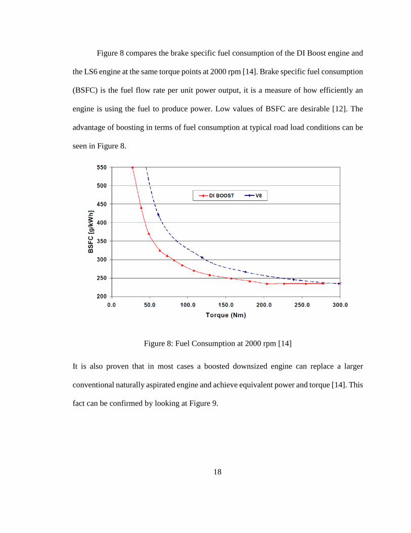
Figure 8 compares the brake specific fuel consumption of the DI Boost engine and

the LS6 engine at the same torque points at 2000 rpm [14]. Brake specific fuel consumption

(BSFC) is the fuel flow rate per unit power output, it is a measure of how efficiently an

engine is using the fuel to produce power. Low values of BSFC are desirable [12]. The

advantage of boosting in terms of fuel consumption at typical road load conditions can be

seen in Figure 8.

Figure 8: Fuel Consumption at 2000 rpm [14]

It is also proven that in most cases a boosted downsized engine can replace a larger

conventional naturally aspirated engine and achieve equivalent power and torque [14]. This

fact can be confirmed by looking at Figure 9.

18

(a)

(b)

Figure 9: Comparison of Naturally Aspirated and Turbocharged Downsized Engines (a)Power (HP) (b) Torque (lb-ft) [14]

19

2.3.2 Electric Machines

One of the major energy converters used in an HEV, other than the engine, is the

electric motor [15]. Electric motors convert electricity to mechanical energy and can also

act as generators and convert mechanical energy to electrical energy. Some of the EMs

require alternating current (AC) to operate, which is provided to the EM by an inverter. An

Inverter, is an electronic device or circuitry that changes direct current (DC) from the

battery pack to alternating current (AC). The conversion of the power from the battery pack

to mechanical and vice-versa depends of the performance of the system that includes the

motor and the inverter. The aspect of the EMs to convert energy 2-ways aspect, is

especially helpful in a parallel architecture as one component of the vehicle solves two

purposes, i.e. convert the mechanical energy from the engine to electricity to charge the

battery, and also convert the electricity from the battery pack into mechanical energy in

order to power the wheels. This ultimately helps in reducing the overall weight of the

vehicle. A major advantage of the electric motor in hybrid electric drive is that torque

generation is very quick and accurate [16]. This section of the thesis discusses the major

kinds of electric machines used in HEVs and their typical performance characteristics.

There are four basic types of motors that can be used in an EV or a HEV: direct-

current motor (DC), induction motor (IM), brushless permanent-magnet motor (PM) and

switched reluctance motor (SRM).Figure 10 illustrates the cross-sections of the previously

mentioned motor types [15].

20

Figure 10: Industrial and Traction Motors’ Cross-Section (a) DC Motor (b) IM (c) PM

Brushless Motor (d) SRM [15]

Figure 11 shows a standard operational characteristic of how torque varies with

respect to speed in any electric motor. Constant torque (or force) region and constant power

region are the two major regions that this typical characteristic curve can be distributed

into. Within the constant torque region the electric motor provides its constant rated torque

up to its base speed. At the base speed the motor reaches its rated power limit. The

operation beyond the base speed is called constant power region. In this region the motor

provides rated power up to its maximum speed. This is obtained by reducing the field flux

of the motor and, therefore, is also known as the ‘field- weakening region’ [17].

21

Figure 11: Typical Motor Torque vs. Speed Characteristic [15]

According to exhaustive research done by [15] it has been observed that

investigations on the SRMs, IMs, and PM motors are increasing while those on DC motors

are decreasing. DC motors work on the principle of magnets; like poles repel and unlike

poles attract. The brushed DC electric motor generally consists of windings in the rotor and

permanent magnets in the stator. DC motors generate torque directly from the DC power

supplied to the motor by using internal commutation, stationary magnets, and the rotating

electrical magnets. One advantage of using a DC motor in HEVs are the simple controls

associated with the machine [15]. Some of the disadvantages to DC motors include bulky

construction, low efficiency, low reliability, and the mechanical commutator (brush) which

increases the maintenance cost on these machines [15]. All the previously mentioned

disadvantages make it hard to use DC motors in HEVs.

22

Figure 12: Typical Switched Reluctance Motor Torque vs. Speed Characteristic [15]

Switched reluctance motor is a type of stepper motor and unlike DC motor, the

power in an SRM is delivered to the windings in the stator rather than the rotor. The direct

current in a SRM generally switches turns in the stators windings. The rotor in a SRM is

made of permanent magnets. Because the rotor is out of line with the magnetic field of the

stator, a torque is produced to minimize the air gap and makes the magnetic field

symmetrical [16]. Figure 12 illustrates the typical SRM torque vs. speed characteristic.

From Figure 12 it can be seen that SRMs have a rather long constant power region apt for

HEV application. Some of the advantages that relate to these motors include: simple and

rugged construction, fault-tolerant operation, simple control, and as previously mentioned

SRMs have an outstanding torque-speed characteristic. Other than these advantages

acoustic noise generation, torque ripple, special converter topology, and excessive bus

23

current ripple are some of the disadvantages associated with SRMs. Acceptable solutions

to the above disadvantages are needed to achieve a viable SRM-based HEV. Nevertheless,

SRM is a solution that is actually envisaged for HEV applications [15].

Induction Motors, unlike DC and SR motors, run on alternating current (AC). The

electric current in an IM is supplied to the stator and further electricity is inducted in the

rotor by magnetic induction rather than direct electric connection. Figure 13 illustrates a

typical induction motor torque-speed curve, which is slightly different than the typical

electric motor curve. The curve consists of an additional “high-speed” region, which begins

at the motors critical speed beyond which if the motor is operated at maximum current the

motor will stall. The critical speed of an IM is typically two times the synchronous base

speed where the motor reaches its breakdown torque. The presence of a breakdown torque

limits an IM’s extended constant-power operation [15].

Figure 13: Typical Induction Motor Torque vs. Speed Characteristic [15]

24

Advantages pertaining to induction motors are: high reliability, ruggedness, low

maintenance, low cost, and ability to operate in hostile environment. These qualities make

IMs one of the most accepted candidates for application in HEVs [15]. Other than the

advantages, some of the disadvantages for IMs are: high energy loss, low efficiency, low

power factor, and low inverter-usage factor, which is more serious for the high speed, large

power motor. Also, IMs efficiency is inherently lower than that of permanent magnet

motors, due to the absence of rotor winding and rotor copper losses [15]. To improve the

IM drive’s efficiency, a new generation of control techniques have been proposed. Also,

to extend the constant-power region, multi-phase pole changing IM drives have been

suggested [15].

Figure 14: Typical Permanent Magnet Brushless Motor Torque vs. Speed Characteristic [15]

Permanent magnet (PM) brushless motors utilize alternating current just like

induction motors. It is called permanent magnet brushless because the armature has no

25

brushes connected to it and the rotor consists of a permanent magnet. Magnetic field is

generated by the stator, which takes alternative supply from a DC source. The rotor moves

because of the interaction with the magnetic field generated by the stator [16]. Figure 14

illustrates the typical PM brushless motor’s torque-speed performance characteristics.

From Figure 14 it is evident that PM brushless motors have a relatively shorter constant-

power region as compared to the other motors discussed earlier in this section. The shorter

constant-power region of these motors is due to their rather limited field weakening

capability, resulting from the presence of the PM Field (the fixed PM limit their extended

speed range). Another disadvantage is that it is costlier due to the presence of permanent

magnet [17] ,[16].

Compared to IM’s, PM brushless motors are currently better contenders for use in

HEVs. This is due to their following advantages: high power density, higher efficiency,

and the ability to dissipate heat to the surroundings with a higher efficiency. The PM

brushless motor is thus most suited for HEVs [15].

2.4 Scalable Approach to HEV modeling

Increasing demand for HEV designs require automated modeling and simulation

tools to construct a design space search. Composability and scalability are highly desirable

in these simulators to provide design candidates. This section scans over different energy

converter scaling approaches adopted by researchers and simulators in the past. This

section also includes an in-depth Willans line scaling model for engines and electric

machines. The prior knowledge to understand Willans line model is also mentioned.

26

2.4.1 Scaling Methods

The Powertrain System Analysis Toolkit (PSAT) is a “forward-looking” model,

PSAT allows users to simulate more than 200 pre-defined configurations, including

conventional, pure electric, fuel cell, and hybrids (parallel, series, power split, series-

parallel). The simulator was developed by Argonne National Laboratory (ANL) and

sponsored by the U.S. Department of Energy (DOE) [18]. ADvanced VehIcle SimulatOR

(ADVISOR) is another simulator but unlike PSAT, ADVISOR is a “backward-looking”

simulator, which can be used for the analysis of performance, fuel economy, and emissions

of conventional, electric, hybrid electric, and fuel cell vehicles. ADVISOR was developed

by U.S. National Renewable Laboratory (NREL) [18]. ADVISOR and PSAT are based in

MATLAB/Simulink environment. Both the simulators, utilize engine’s fuel consumption

and efficiency data to evaluate the overall performance of the vehicle. The data within these

simulators is in the form of look-up tables within MATLAB. Based on the maximum power

and efficiency of the desired engine, both the simulators (PSAT and ADVISOR) employ

linear scaling strategy, which allows the user to conduct parametric studies for the options

that are not on the list of available engines within the simulator. In other words, when a

chosen engine has either different maximum power rating or different peak efficiency from

the default values, their efficiency maps will be proportionally scaled with the efficiency

ratio. Speed and torque indices of the efficiencies are also scaled based on the required

maximum power of the engine.

Assanis et al. [19] apply a different scaling strategy to a high-fidelity turbocharged

compression-ignition engine simulator. The scaling done by [19] provides better prediction

27

of the fuel consumption and efficiency data for the scaled engines because the methodology

considers non-linearity factors. The high-fidelity of the method makes it more complicated

as it requires more knowledge of many engine parameters.

J. Pries and H. Hoffmann [20] provide a way that allows magnetic and thermal

scaling of electric machines. The method adopted by [20] involves developing partial

differential equations describing electromagnetic and thermal dynamics of the machine,

which incorporate non-linear magnetic behavior such as saturation and hysteresis. The

high-fidelity of the method makes it more complicated than the scope of this project.

In the past, Willans line model has been used to describe an approximate linear

relationship between brake mean effective pressure and fuel consumption of an ICE. [12]

Rizzoni, Guzzella and Baumann [11] extended the already existing Willans line model to

describe generalized energy converters (engines and electric motors). Based on known

steady state efficiency data of the reference machine, the efficiency of a new machine in

the same category can be estimated using this scaling approach.

The Willans line model consists of an affine relationship which relates the available

energy, that is, the energy that is theoretically available for conversion, to the useful energy

that is actually present at the output of the energy converter. The relationship is described

by two coefficients: the slope, or intrinsic energy conversion efficiency e; and the vertical

axis intercept Wloss. In an ICE, e corresponds to the energy conversion efficiency that is

characteristic of a specific cycle (Otto, Diesel, Miller, etc.) and Wloss represents the

frictional and auxiliary losses [11]. The relationship is described in Equation (2.2) and a

representation of that relation is shown in Figure 15.

28

out in lossW eW W= − (2.2)

Figure 15: Input-Output Relationship of an Energy Converter [11]

The actual energy conversion efficiency of an energy converter can be defined as the ratio

of output work done to the input work done by the converter as described in Equation (2.3).

out

in

WW

η = (2.3)

Relating equations (2.2) & (2.3) indicate that the actual conversion efficiency is a function

of the operating conditions of the converter and that it is maximum in that operating region

where the ratio of energy losses to input energy is smallest.

in loss loss

in in

eW W WeW W

η−

= = − (2.4)

Further application of the Willans line concept to the engine and electric machines scaling,

and also the method adopted to predict e and Wloss for the two is energy converters is

explained in the section.

29

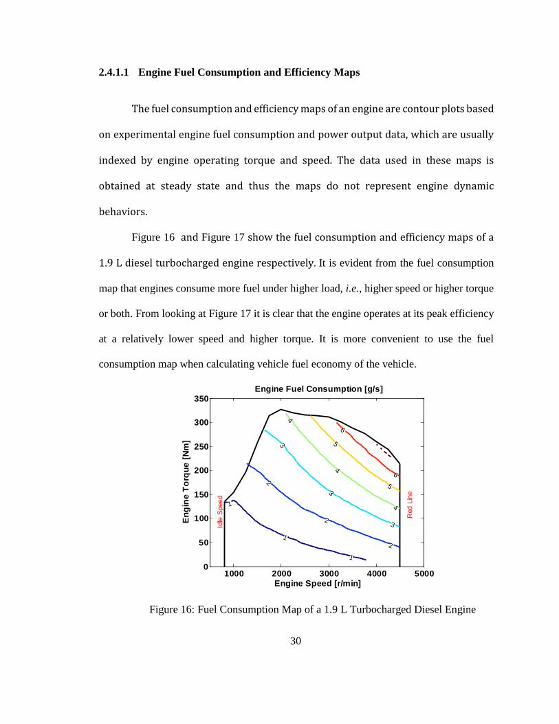
2.4.1.1 Engine Fuel Consumption and Efficiency Maps

The fuel consumption and efficiency maps of an engine are contour plots based

on experimental engine fuel consumption and power output data, which are usually

indexed by engine operating torque and speed. The data used in these maps is

obtained at steady state and thus the maps do not represent engine dynamic

behaviors.

Figure 16 and Figure 17 show the fuel consumption and efficiency maps of a

1.9 L diesel turbocharged engine respectively. It is evident from the fuel consumption

map that engines consume more fuel under higher load, i.e., higher speed or higher torque

or both. From looking at Figure 17 it is clear that the engine operates at its peak efficiency

at a relatively lower speed and higher torque. It is more convenient to use the fuel

consumption map when calculating vehicle fuel economy of the vehicle.

Figure 16: Fuel Consumption Map of a 1.9 L Turbocharged Diesel Engine

1000 2000 3000 4000 50000

50

100

150

200

250

300

350

Idle

Spe

ed

Red

Lin

e

1

1

1

2

2

2

3

3

3

4

4

4

5

5

6

6

Engine Speed [r/min]

Eng

ine

Torq

ue [N

m]

Engine Fuel Consumption [g/s]

30

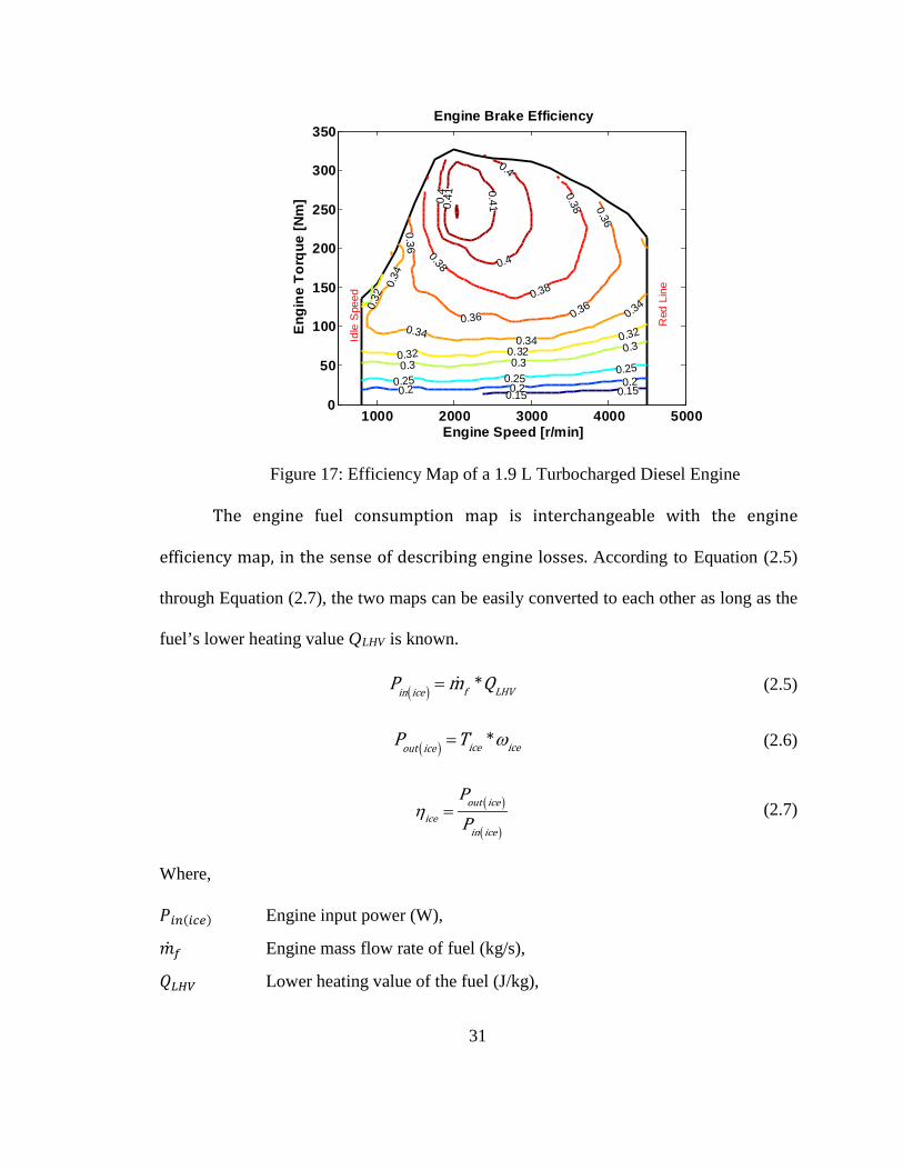
Figure 17: Efficiency Map of a 1.9 L Turbocharged Diesel Engine

The engine fuel consumption map is interchangeable with the engine

efficiency map, in the sense of describing engine losses. According to Equation (2.5)

through Equation (2.7), the two maps can be easily converted to each other as long as the

fuel’s lower heating value QLHV is known.

( ) *f LHVin iceP m Q= (2.5)

( ) *ice iceout iceP T ω= (2.6)

( )

( )

out iceice

in ice

PP

η = (2.7)

Where,

𝑃𝑃𝑖𝑖𝑖𝑖(𝑖𝑖𝑖𝑖𝑖𝑖) Engine input power (W),

�̇�𝑚𝑓𝑓 Engine mass flow rate of fuel (kg/s),

𝑄𝑄𝐿𝐿𝐿𝐿𝐿𝐿 Lower heating value of the fuel (J/kg),

1000 2000 3000 4000 50000

50

100

150

200

250

300

350

Idle

Spe

ed

Red

Lin

e

0.15 0.150.2 0.2 0.20.25 0.250.250.3 0.3

0.3

0.32

0.32 0.320.32

0.34

0.340.34

0.34

0.36

0.36 0.360.36

0.38

0.38

0.380.4

0.4

0.4

0.410.41

Engine Speed [r/min]

Eng

ine

Torq

ue [N

m]

Engine Brake Efficiency

31

𝑃𝑃𝑜𝑜𝑜𝑜𝑜𝑜(𝑖𝑖𝑖𝑖𝑖𝑖) Engine output power (W),

𝑇𝑇𝑖𝑖𝑖𝑖𝑖𝑖 Engine torque (N-m),

𝜔𝜔𝑖𝑖𝑖𝑖𝑖𝑖 Engine speed (rad/s),

𝜂𝜂𝑖𝑖𝑖𝑖𝑖𝑖 Engine efficiency.

2.4.1.2 Willans Line Model for Engines

The input-output powers and the intrinsic efficiency of an engine, as viewed

for the Willans line model is described in Equation (2.8).

( ) ( ) ( )*iceout ice in ice loss iceP e P P= − (2.8)

In order to eliminate sizing effects, the engine speed and the torque are substituted by the

normalized variables including the mean piston speed and the mean effective pressures.

According to [12], torque is a valuable measure of a particular engine’s ability to do work

which, depends on engine size. A more useful relative engine performance measure is

obtained by dividing the work per cycle by the cylinder volume displaced per cycle as

expressed in Equation (2.11). Also, [12] states that mean piston speed is often a more

appropriate parameter than crank rotational speed for correlating engine behavior as a

function of speed. The instantaneous piston velocity Cm is obtained from the Equation

(2.9). Figure 18 represents the physical parameters (stroke length and displacement

volume) of the engine that have been used in the Equation (2.9) through Equation (2.11).

( )* ice

m ice

SC ωπ

= (2.9)

32

( )4 LHV f

ma iced ice

Q mPVπ

ω=

(2.10)

( )4 ice

me iced

TPVπ

= (2.11)

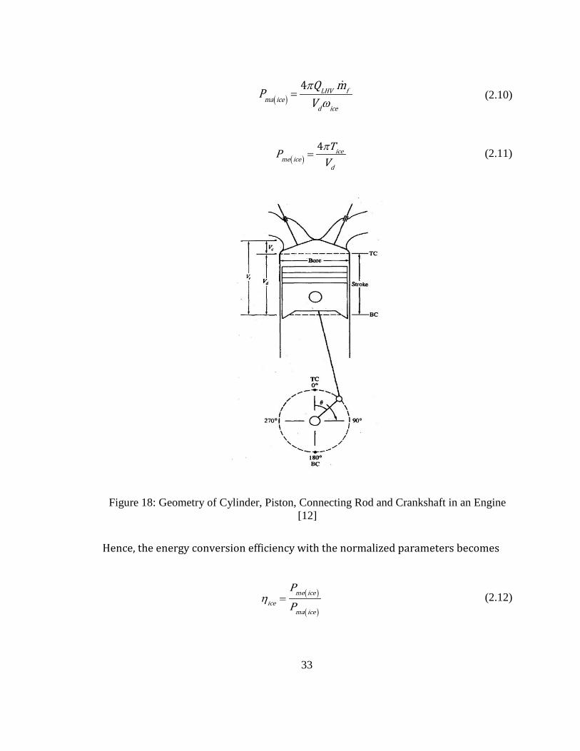
Figure 18: Geometry of Cylinder, Piston, Connecting Rod and Crankshaft in an Engine [12]

Hence, the energy conversion efficiency with the normalized parameters becomes

( )

( )

me iceice

ma ice

PP

η = (2.12)

33

Now, the input-output relationship according to Willans line model for engines can

be written in the format represented in Equation (2.13).

( ) ( ) ( )*iceme ice ma ice ml iceP e P P= − (2.13)

Once, Pma(ice) and Pme(ice) are calculated at each operating speed, the intrinsic efficiency eice

and the mean friction pressure Pml(ice) are approximated to be functions of Cm(ice) and Pma(ice)

as represented in Equation (2.14) and Equation (2.15) respectively.

( ) ( ) ( ) ( ) ( )( ) ( ) ( ) ( )( ) ( )2

00 01 02 10 11ice ice ice m ice ice m ice ice ice m ice ma icee e e C e C e e C P= + + − + (2.14)

( ) ( ) ( ) ( )2

0 2ml ice ml ice ml ice m iceP P P C= + (2.15)

e10(ice) and e11(ice) in Equation (2.14) are often close to zero, reducing eice to a function of

Cm(ice) alone. The wide-open throttle mean effective pressure curve of engines is

identified as shown in Equation (2.16).

( ) ( ) ( )

3

max0

iice maxi ice m ice

i

P P C=

=∑ (2.16)

In Equations (2.8) through (2.16),

𝐶𝐶𝑚𝑚(𝑖𝑖𝑖𝑖𝑖𝑖) Engine mean piston speed (m/s),

𝑃𝑃𝑙𝑙𝑜𝑜𝑙𝑙𝑙𝑙(𝑖𝑖𝑖𝑖𝑖𝑖) Engine power losses (W),

𝑆𝑆 Engine stroke length (m),

𝑃𝑃𝑚𝑚𝑚𝑚(𝑖𝑖𝑖𝑖𝑖𝑖) Engine theoretically available mean effective pressure (Pa),

𝑉𝑉𝑑𝑑 Engine displacement (m3),

34

𝑃𝑃𝑚𝑚𝑖𝑖(𝑖𝑖𝑖𝑖𝑖𝑖) Engine actual mean effective pressure (Pa),

𝑃𝑃𝑚𝑚𝑙𝑙(𝑖𝑖𝑖𝑖𝑖𝑖) Engine mean friction pressure (Pa),

𝑒𝑒𝑖𝑖𝑖𝑖𝑖𝑖 Engine intrinsic energy conversion efficiency - transferring losses (%),

𝑒𝑒𝑖𝑖𝑖𝑖(𝑖𝑖𝑖𝑖𝑖𝑖) Scaling coefficients of engine intrinsic energy conversion efficiency eice,

𝑃𝑃𝑚𝑚𝑙𝑙𝑖𝑖(𝑖𝑖𝑖𝑖𝑖𝑖) Scaling coefficients of engine mean friction pressure,

𝑃𝑃max(𝑖𝑖𝑖𝑖𝑖𝑖) Engine wide-open throttle mean effective pressure (Pa),

𝑃𝑃maxi(𝑖𝑖𝑖𝑖𝑖𝑖) Scaling coefficients of wide-open throttle mean effective pressure.

Two important things need to be noted when applying the Willans line model. First,

the scaled machine and the scaling machine should be from the same class of engines, e.g.

SI or CI engines, turbo/supercharged engines. Further, when generating the scaling

coefficients, the user should curve fit over a wide range of the scaling variable of Cm(ice) so

that during the subsequent use of the model, the efficiency of the scaled engine is not

obtained by doing extrapolation [11].

2.4.1.3 Electric Machine Efficiency Map

The efficiency map which is not restricted to the machine type finds extensive

applications in solving automotive design and control problems. Similar to the engine

efficiency map, the EM efficiency map also represents static empirical efficiency data

as contours on a torque-speed plot. Figure 19 shows the efficiency map of a brushless

PM motor with a rotor volume of 1.4 L.

35

Figure 19: PM Brushless Motor with a 1.4 L Rotor Efficiency Map

The flat segment in the maximum torque curve as mentioned in Section 2.3.2 is called

constant torque region and the hyperbolic decaying segment reflects the flux

weakening region. Unlike Figure 11 it can be seen that the torque in Figure 19 is

positive as well as negative. The positive torque region shows the propulsion aspect

of the EM, i.e. the part which converts electrical energy from the battery to mechanical

energy which moves the vehicle. The negative torque region shows the regenerative

aspect of the EM, i.e. the part where the motor converts mechanical energy during

braking from the wheels to electrical energy to charge the battery pack in a HEV or

an EV. The EM behavior in the generating mode (negative EM torque region) is usually

different from those in the motoring mode (positive EM torque region), but engineers

may consider they are the same, i.e., symmetric about the zero torque line for

0 2000 4000 6000 8000-300

-200

-100

0

100

200

300

0.7

0.7

0.7

0.7

0.7

0.70.

75

0.75

0.75

0.75

0.75

0.75

0.8

0.8

0.8

0.8

0.8

0.8

0.8

0.85

0.85

0.85

0.85

0.85

0.85

0.85

0.850.85 0.85

0.87

0.87

0.87

0.87

0.87

0.87

0.87

0.870.870.87 0.87

0.89

0.89

0.89

0.89

0.890.89

0.89

0.890.890.89 0.89 0.89

0.91

0.91

0.91

0.91

0.91 0.91

0.91

0.910.910.910.91 0.91 0.91

0.920.92

0.92

0.92 0.92 0.920.920.920.92

0.920.92

0.92

0.930.93

0.93

0.93 0.93 0.93

0.930.930.93

0.930.93

0.93

0.94

0.94

0.94

0.94 0.94

0.940.940.94

0.940.94

0.95

0.95

Speed [RPM]

Torq

ue [N

m]

Efficiency

36

simplicity. In general, the highest efficiency of an EM is located at the higher power

region.

2.4.1.4 Willans Line Model for Electric Machines

As mentioned earlier, the Willans line model is also applicable in describing

electric machines. The input-output powers and the efficiency of an EM in the

motoring mode are described in Equation (2.17) through Equation (2.19).

( ) *in emP U I= (2.17)

( ) *em emout emP T ω= (2.18)

( )

( ) out em

emin em

P

Pη = (2.19)

Using the Willans line concept, the EM input-output relationship can be represented

as is done in Equation (2.20).

( ) ( ) ( )*emout em in em loss emP e P P= − (2.20)

Applying the normalized variables of the mean rotor speed and the air gap shear

stresses, we obtain:

( ) r emm emC r ω= (2.21)

( )*

2ma emr em

U IPV ω

= (2.22)

37

( ) 2*em

me emr

TPV

= (2.23)

( )

( )

me emem

ma em

PP

η = (2.24)

( ) ( ) ( )*emme em ma em ml emP e P P= − (2.25)

The physical parameters (rotor radius and rotor length) used in Equation (2.21)

through Equation (2.23) are described in Figure 20.

Figure 20: Rotor Physical Parameters

Noting the success of the polynomial models for the engine, polynomials in Cm(em) were

initially selected to model eem and Pml(em) of the EM according to [11]. Again according to

[11] the simulation results showed that fourth order polynomials capture the behavior of

eem and Pml(em) with sufficient accuracy and without excessive coefficients, the expressions

for which are illustrated in Equation (2.26) and Equation (2.27) respectively.

( ) ( )

4

00

iem i em m em

i

e e C=

=∑ (2.26)

( ) ( ) ( )

4

0

iml em mli em m em

i

P P C=

=∑ (2.27)

38

In Equation (2.17) through Equation (2.27),

𝑃𝑃𝑖𝑖𝑖𝑖(𝑖𝑖𝑚𝑚) EM input power (W),

𝑃𝑃𝑙𝑙𝑜𝑜𝑙𝑙𝑙𝑙(𝑖𝑖𝑚𝑚) EM power losses (W),

𝑈𝑈 EM voltage supply (V),

𝐼𝐼 EM current supply (A),

𝑃𝑃𝑜𝑜𝑜𝑜𝑜𝑜(𝑖𝑖𝑚𝑚) EM output power (W),

𝐶𝐶𝑚𝑚(𝑖𝑖𝑚𝑚) EM mean rotor speed (m/s),

𝑟𝑟 EM rotor radius (m),

𝑃𝑃𝑚𝑚𝑚𝑚(𝑖𝑖𝑚𝑚) EM theoretical air gap shear stress (Pa),

𝑉𝑉𝑟𝑟 EM rotor volume (m3),

𝑃𝑃𝑚𝑚𝑖𝑖(𝑖𝑖𝑚𝑚) EM actual air gap shear stress (Pa),

𝑃𝑃𝑚𝑚𝑙𝑙(𝑖𝑖𝑚𝑚) EM mean friction pressure (Pa),

𝑒𝑒𝑖𝑖𝑚𝑚 EM intrinsic energy conversion efficiency - transferring losses (%),

𝑒𝑒𝑖𝑖𝑖𝑖(𝑖𝑖𝑚𝑚) Scaling coefficients of EM intrinsic energy conversion efficiency eice,

𝑃𝑃𝑚𝑚𝑙𝑙𝑖𝑖(𝑖𝑖𝑚𝑚) Scaling coefficients of EM mean friction pressure,

The Willans line model for the electric machines also allows building the

scalable models within the same category, such as induction EM, permanent magnet

synchronous EM and switched reluctance EM. One may refer to engine’s Willans line

model for detailed description of model application and restrictions.

2.5 EcoSIM

The Ohio State EcoCAR team has developed an energy-based model called

EcoSIM to develop control strategies for the vehicle over the past 8 years. This model

allows the team to see how different strategies affect fuel economy and performance. This

39

chapter contains a very basic explanation of this model. A more detailed description can

be found in [4].

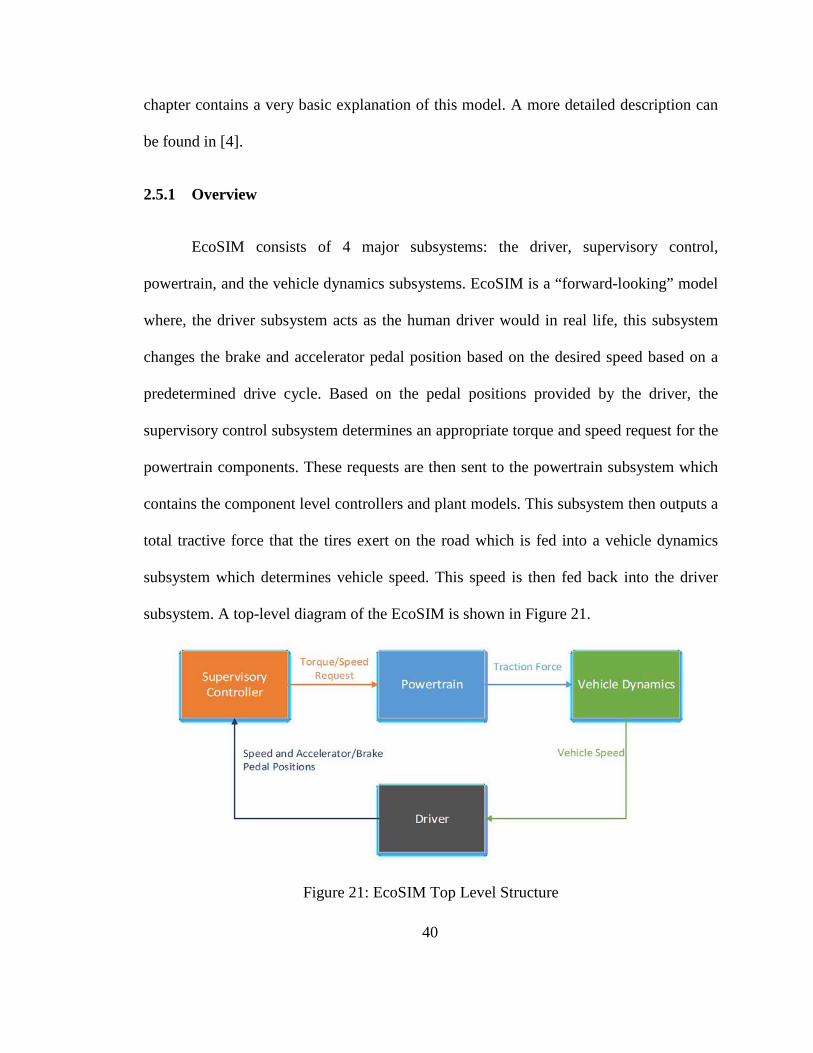
2.5.1 Overview

EcoSIM consists of 4 major subsystems: the driver, supervisory control,

powertrain, and the vehicle dynamics subsystems. EcoSIM is a “forward-looking” model

where, the driver subsystem acts as the human driver would in real life, this subsystem

changes the brake and accelerator pedal position based on the desired speed based on a

predetermined drive cycle. Based on the pedal positions provided by the driver, the

supervisory control subsystem determines an appropriate torque and speed request for the

powertrain components. These requests are then sent to the powertrain subsystem which

contains the component level controllers and plant models. This subsystem then outputs a

total tractive force that the tires exert on the road which is fed into a vehicle dynamics

subsystem which determines vehicle speed. This speed is then fed back into the driver

subsystem. A top-level diagram of the EcoSIM is shown in Figure 21.

Figure 21: EcoSIM Top Level Structure

40

Within the powertrain subsystem, engines’ and electric machines’ controllers and

plant models are stored. The engine plant model includes simplified dynamics of the engine

torque and speed response and output the actual torque and speed. With this torque and speed

it is possible to find the engine efficiency and engine fuel consumption rate based on the maps

which are stored within EcoSIM in the form of look-up tables. Similarly, once the EM torque

and speed commands are determined, they get passed to the EM plant model which contains

simplified dynamics. The plant model then outputs a torque and speed. From this, the efficiency

of the EM can be determined using stored efficiency maps. It is these fuel consumption and

efficiency maps of the engines and electric machines that the EcoCAR 3 team would replace

with different size engine and EM data to test different components.

41

CHAPTER 3: SCALING METHODS

3.1 Introduction

The methods utilized by the developed tools to scale engine and electric machine’s

data, which will be used by the EcoCAR 3 team to test different size components within

EcoSIM, and the assumptions made during scaling of these energy converters data are

described in this chapter.

3.2 Engine Scaling

The engine-scaling tool was developed within MATLAB. The tool allows the user

to generate fuel consumption and power output data of an engine of desired size given the

fuel consumption data of an already existing engine (of different size) belonging to the

same category. The same category restriction means if the user wants to generate data for

a certain type of engine (naturally aspirated, super/turbo-charged, gasoline direct injection,

SI, CI, etc.) the tool will require the fuel-consumption data for that same type of already

existing engine. This requirement of the tool has been explained in Section 2.3.1 of this

thesis. Any change in the engine technology affects the engine performance significantly.

The scaling method adopted by the engine-scaling tool for this project is very similar to

the Willans line model, which has been explained in section 2.4.1.2. The difference

between the approach adopted by this project and the Willans line model is that this tool

assumes the efficiencies of engines with similar technologies to be the same. Due to this

assumption the tool developed can scale engines that are within thirty percent size range of

the baseline engine. The accuracy of the predicted data decreases as the size difference

42

between the baseline engine and the required engine increases more than thirty percent.

Since, the difference between displacements of the engines under consideration by the

EcoCAR 3 team is within thirty percent, this restriction of the scaling tool is not of concern

to the EcoCAR 3 team. The step-by-step scaling of a 1.6 L Naturally Aspirated (NA) SI

engine to a 1.8 L NA-SI engine and the comparison between the 2 engines is illustrated

further in this section.

As mentioned earlier, the engine-scaling tool requires fuel consumption data of

same type already existing engine. Table 1 shows the technological aspect and the physical

parameters of the existing engine, the data for which was extracted from PSAT’s

component library. The Figure 22 shows how the fuel consumption of the 1.6 L engine

varies with respect to torque and speed. At each indexed point where the fuel consumption

data was available, the power output of the engine was determined using Equation (3.1)

and the corresponding map is shown in Figure 23.

𝑃𝑃𝑜𝑜𝑜𝑜𝑜𝑜(𝑖𝑖𝑖𝑖𝑖𝑖) = 𝑇𝑇𝑖𝑖𝑖𝑖𝑖𝑖 ∙ 𝜔𝜔𝑖𝑖𝑖𝑖𝑖𝑖 (3.1)

Table 1: Specifications for the Existing Engine

Engine Technology Engine Displacement (Vd) (L)

Engine Stroke Length (S) (mm)

Naturally Aspirated 1.6 90

43

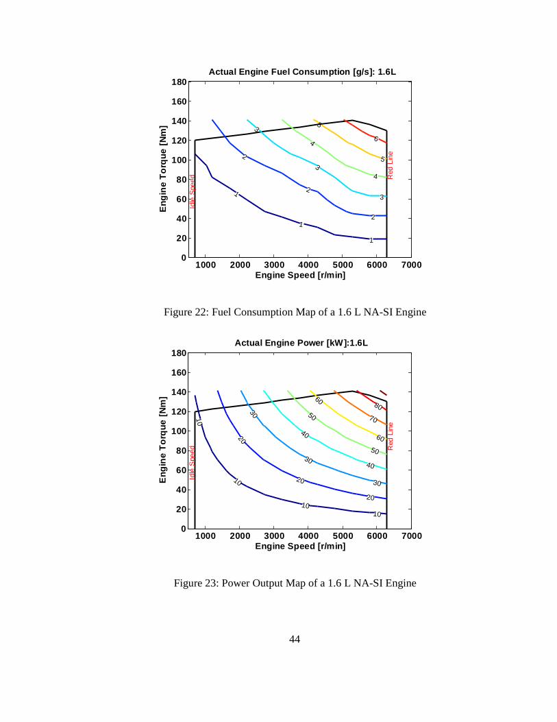
Figure 22: Fuel Consumption Map of a 1.6 L NA-SI Engine

Figure 23: Power Output Map of a 1.6 L NA-SI Engine

1000 2000 3000 4000 5000 6000 70000

20

40

60

80

100

120

140

160

180

Idle

Spe

ed Red

Lin

e

1

1

1

2

2

2

3

3

3

4

4

5

5

6

Engine Speed [r/min]

Eng

ine

Torq

ue [N

m]

Actual Engine Fuel Consumption [g/s]: 1.6L

1000 2000 3000 4000 5000 6000 70000

20

40

60

80

100

120

140

160

180

Idle

Spe

ed Red

Lin

e

10

10

1010

20

20

20

30

30

30

40

40

50

50

60

60

70

80

Engine Speed [r/min]

Eng

ine

Torq

ue [N

m]

Actual Engine Power [kW]:1.6L

44

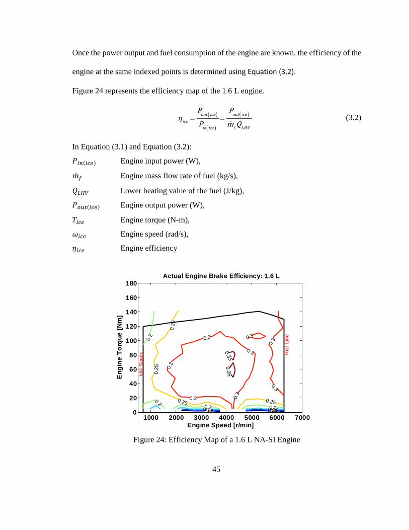
Once the power output and fuel consumption of the engine are known, the efficiency of the

engine at the same indexed points is determined using Equation (3.2).

Figure 24 represents the efficiency map of the 1.6 L engine.

( )

( )

( )η = =

out ice out iceice

f LHVin ice

P P

P m Q (3.2)

In Equation (3.1) and Equation (3.2):

𝑃𝑃𝑖𝑖𝑖𝑖(𝑖𝑖𝑖𝑖𝑖𝑖) Engine input power (W),

�̇�𝑚𝑓𝑓 Engine mass flow rate of fuel (kg/s),

𝑄𝑄𝐿𝐿𝐿𝐿𝐿𝐿 Lower heating value of the fuel (J/kg),

𝑃𝑃𝑜𝑜𝑜𝑜𝑜𝑜(𝑖𝑖𝑖𝑖𝑖𝑖) Engine output power (W),

𝑇𝑇𝑖𝑖𝑖𝑖𝑖𝑖 Engine torque (N-m),

𝜔𝜔𝑖𝑖𝑖𝑖𝑖𝑖 Engine speed (rad/s),

𝜂𝜂𝑖𝑖𝑖𝑖𝑖𝑖 Engine efficiency

Figure 24: Efficiency Map of a 1.6 L NA-SI Engine

1000 2000 3000 4000 5000 6000 70000

20

40

60

80

100

120

140

160

180

Idle

Spe

ed Red

Lin

e

0 05 0 050.1 0.10.15 0.15

0.20.2 0.2

0.2

0.25

0.25

0.25

0.250.3

0.3

0.3

0.3

0.3

0.3

0.3

0.3

0.350.35

Engine Speed [r/min]

Eng

ine

Torq

ue [N

m]

Actual Engine Brake Efficiency: 1.6 L

45

Further the tool converts engine’s torque and speed at every efficiency points to normalized

parameters i.e., engine’s BMEP and mean piston speed respectively. The efficiencies of

the engine at these indexed points are kept constant. Figure 25 shows a map of how the

engine’s efficiency varies with the engine’s BMEP and mean piston speed. The mean

piston speed and the engine’s brake mean effective pressure are calculated using Equation

(3.3) and Equation (3.4) respectively.

=*

30mS NC (3.3)

π=

4100000* d

TBMEPV

(3.4)

In the equations:

Cm Engine mean piston speed (m/s)

S Engine stroke length (m)

N Engine speed (RPM)

BMEP Engine brake mean effective pressure (bar)

T Engine torque (Nm)

Vd Engine’s displacement volume (m3)

46

Figure 25: Normalized Efficiency Map of a NA-SI Engine

The data shown in the efficiency map in Figure 25, with the normalized parameters can be

utilized to scale any engine with a displacement that is within thirty percent range of the

1.6 L engine. As an example the 1.6 L engine has been scaled to another 1.8 L engine, the

specifications for which are described in Table 2.

Table 2: Specifications for the Predicted Engine

Engine Technology Engine Displacement (Vdnew) (L)

Engine Stroke Length (Snew)(mm)

Naturally Aspirated 1.8 88.3

0 5 10 15 200

2

4

6

8

10

12

0 05 0 050.1 0.10.15 0.15

0.2

0.2 0.2

0.2

0.25

0.250.

25

0.25

0.250.3

0.3

0.3

0.3

0.3

0.3

0.30.3

0.3

0.350.35

Mean Piston Speed [m/s]

Eng

ine

BM

EP

[Bar

]

Normalized Engine Brake Efficiency

47

Figure 26: Predicted Efficiency Map of a 1.8L NA-SI Engine

Figure 26 illustrates the brake efficiency of the new NA 1.8 L SI engine. The

normalized terms i.e. the BMEP and mean piston speed of the 1.6 L engine were used in

conjunction with the physical parameters of the 1.8 L engine to determine the new torque

and speed indices for the efficiencies. Equation (3.5) and Equation (3.6) describe the

conversion of engine BMEP to torque and mean piston speed to engine speed respectively.

π=

*10000*4 *

d newnew

BMEP VT (3.5)

=

1*30*

.104719

mnew

new

RPMCN RPMS rad

s

(3.6)

1000 2000 3000 4000 5000 6000 70000

20

40

60

80

100

120

140

160

180

Idle

Spe

ed Red

Lin

e

0 05 0 050.1 0.10.15 0.15

0.20.2 0.2

0.2

0.25

0.25

0.25

0.25

0.250.3

0.3

0.3

0.3

0.3

0.3

0.3

0.3

0.3

0.32

0.32

0.320.320.32

0.32

0.33

0.33

0.33

0.33

0.33

0.34

0.34

0.34

0.350.35

Engine Speed [r/min]

Eng

ine

Torq

ue [N

m]

Predicted Engine Brake Efficiency:1.8L

48

Where, 𝑇𝑇𝑖𝑖𝑖𝑖𝑛𝑛 and 𝑁𝑁𝑖𝑖𝑖𝑖𝑛𝑛 are the torque and speed of the newly scaled engine. The converted

torques and speed at each of the indexed efficiency points are used to determine the engine

power output. Figure 27 illustrates the power output map of the 1.8 L engine.

Figure 27: Predicted Power Map of a 1.8L NA-SI Engine

Utilizing the power output and efficiency data points, the fuel consumption of the 1.8L

engine was determined using Equation (3.7) and Figure 28 illustrates the predicted fuel

consumption map of the 1.8 L engine.

( )

η=

*ice LHVf

out ice

QmP

(3.7)

1000 2000 3000 4000 5000 6000 70000

20

40

60

80

100

120

140

160

180

Idle

Spe

ed Red

Lin

e10

10

1010

20

20

20

2030

30

3040

40

40

50

50

60

60

70

70

80

90

Engine Speed [r/min]

Eng

ine

Torq

ue [N

m]

Predicted Engine Power [kW]:1.8L

49

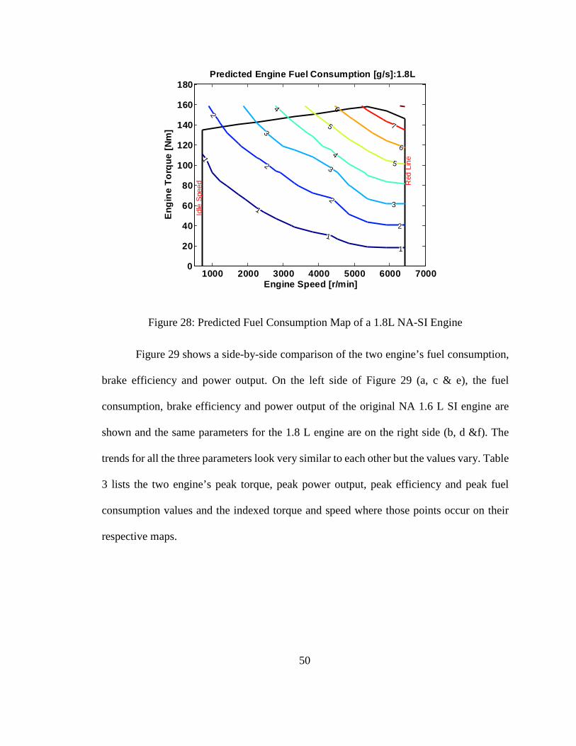
Figure 28: Predicted Fuel Consumption Map of a 1.8L NA-SI Engine

Figure 29 shows a side-by-side comparison of the two engine’s fuel consumption,

brake efficiency and power output. On the left side of Figure 29 (a, c & e), the fuel

consumption, brake efficiency and power output of the original NA 1.6 L SI engine are

shown and the same parameters for the 1.8 L engine are on the right side (b, d &f). The

trends for all the three parameters look very similar to each other but the values vary. Table

3 lists the two engine’s peak torque, peak power output, peak efficiency and peak fuel

consumption values and the indexed torque and speed where those points occur on their

respective maps.

1000 2000 3000 4000 5000 6000 70000

20

40

60

80

100

120

140

160

180

Idle

Spe

ed Red

Lin

e1

1

1

1

2

2

2

2

3

3

3

4

4

5

5

6

6

7

Engine Speed [r/min]

Eng

ine

Torq

ue [N

m]

Predicted Engine Fuel Consumption [g/s]:1.8L

50

(a) (b)

(c) (d)

(e) (f)

Figure 29: Actual 1.6 L and Predicted 1.8 L engine (a-b) Fuel consumption, (c-d) Efficiency and (e-f) Power Output comparison

1000 2000 3000 4000 5000 6000 70000

20

40

60

80

100

120

140

160

180

Idle

Spe

ed Red

Lin

e

1

1

1

2

2

2

3

3

3

4

4

5

5

6

Engine Speed [r/min]

Eng

ine

Torq

ue [N

m]

Actual Engine Fuel Consumption [g/s]: 1.6L

1000 2000 3000 4000 5000 6000 70000

20

40

60

80

100

120

140

160

180

Idle

Spe

ed Red

Lin

e1

1

1

1

2

2

2

2

3

3

3

4

4

5

5

6

6

7

Engine Speed [r/min]

Eng

ine

Torq

ue [N

m]

Predicted Engine Fuel Consumption [g/s]:1.8L

1000 2000 3000 4000 5000 6000 70000

20

40

60

80

100

120

140

160

180

Idle

Spe

ed Red

Lin

e

0 05 0 050.1 0.10.15 0.15

0.20.2 0.2

0.2

0.25

0.25

0.25

0.250.3

0.3

0.3

0.3

0.3

0.3

0.3

0.3

0.350.35

Engine Speed [r/min]

Eng

ine

Torq

ue [N

m]

Actual Engine Brake Efficiency: 1.6 L

1000 2000 3000 4000 5000 6000 70000

20

40

60

80

100

120

140

160

180

Idle

Spe

ed Red

Lin

e

0 05 0 050.1 0.10.15 0.15

0.20.2 0.2

0.2

0.25

0.250.

25

0.25

0.250.3

0.3

0.3

0.3

0.3

0.3

0.3

0.3

0.3

0.32

0.32

0.32

0.320.32

0.32

0.33

0.33

0.33

0.33

0.33

0.34

0.34

0.34

0.350.35

Engine Speed [r/min]

Eng

ine

Torq

ue [N

m]

Predicted Engine Brake Efficiency:1.8L

1000 2000 3000 4000 5000 6000 70000

20

40

60

80

100

120

140

160

180

Idle

Spe

ed Red

Lin

e

10

10

1010

20

20

20

30

30

30

40

40

50

50

60

60

70

80

Engine Speed [r/min]

Eng

ine

Torq

ue [N

m]

Actual Engine Power [kW]:1.6L

1000 2000 3000 4000 5000 6000 70000

20

40

60

80

100

120

140

160

180

Idle

Spe

ed Red

Lin

e10

10

1010

20

20

20

20

30

30

30

40

40

40

50

50

60

60

70

70

80

90

Engine Speed [r/min]

Eng

ine

Torq

ue [N

m]

Predicted Engine Power [kW]:1.8L

51

Table 3: Original vs. Scaled Engine Parameters Comparison

NA 1.6 L SI engine NA 1.8 L SI engine (predicted)

Torque (Nm) Speed (RPM) Torque (Nm)

Speed (RPM)

Peak Torque (Nm) 140.5 140.5 5282 158 158 5384

Peak Power Output (kW) 85 129.3 6300 97.8 145.4 6421

Peak efficiency 35.89 58.8 4264 35.89 66.1 4345.7

Peak Fuel Consumption (g/s) 6.5 129.3 6300 7.45 145.4 6421

Looking at Table 3 and Figure 29 it can be seen that the peak power and peak fuel

consumption of the both the engines occur at the same respective indexed torque and speed.

The peak fuel consumption and peak power output value and also the corresponding

torque-speed indices where these occur are different for both the engines. The 1.8 L engine

has a higher power output and consumes more fuel at its peak points than the 1.6 L engine,

proving the tool is scaling the engine in a correct fashion. The maximum torque of the 1.8

L is higher than the original 1.6 L engine and occurs at a faster speed as well. Peak brake

efficiencies of the two engines is the same due to the constant efficiency assumption of the

tool, while the torque-speed indices for the two engines where the peak efficiency occurs

are different. The 1.8 L engine reaches at its peak efficiency at a higher torque and speed

as compared to the 1.6 L engine.

52

3.3 Electric Machine Scaling

Just like the engine-scaling tool the electric machine (EM) scaling tool was

developed within MATLAB as well. The tool allows the user to generate efficiency and

power output data of an EM of desired size given the efficiency data of an already existing

EM (of different size) belonging to the same category. Using the power output and

efficiency data, the user could also get the power consumption map of the EM. The same

category restriction means if the user wants to generate data for a certain type of EM (DC,

IM, brush-less PM motor etc.) the tool will require the efficiency data for that same type

of already existing engine. This requirement of the tool has been explained in Section 2.3.2

of this thesis-any change in the EM technology affects the EM’s torque-speed

characteristics significantly. The scaling method adopted by the EM scaling tool for this

project is very similar to the Willans line model, which has been explained in Section

2.4.1.4. The difference between the approach adopted by this project and the Willans line

model is that this tool assumes the efficiencies of EMs with similar technologies to be the

same. Due to this assumption the tool developed can scale EMs that are within a certain

percent size range of the baseline EM for which the data is available. The maximum percent

difference between the baseline EM and the to-be scaled EM for accurate results is

unknown. But it is known that the accuracy of the predicted data decreases as the size

difference between the baseline EM and the required EM increases. The step-by-step

scaling of a brush-less PM motor with a 1.4 L rotor by volume to a brush-less PM motor

with a 2.1 L rotor by volume and the comparison between the 2 EMs is illustrated further

in this section.

53

As mentioned earlier, the EM scaling tool requires the energy conversion efficiency

data of same type already existing EM. Table 4 shows the technological aspect and the

physical parameters of the existing EM, Parker-Hannifin’s GVM210-100-TP, the

efficiency and performance data for which was provide to the EcoCAR 2 team by Parker-

Hannifin. Parker-Hannifin evaluated the parameters within a FEA study, which was further

validated by them experimentally.

Table 4: Specifications for the Existing EM

EM Technology Rotor Stack Length (l) (mm)

Rotor Radius (r) (mm)

Brush-less PM motor 100 66.75

Further the physical parameters provided were used to determine the volume of the EM’s

rotor using the Equation (3.8) and found to be 1,369,980 mm3.

π= 2rV r l (3.8)

Figure 30 shows how the energy conversion efficiency of the EM with a 1.4 L rotor varies

with respect to torque and speed. As explained earlier in Section 2.4.1.3 the positive torque

region of Figure 30 illustrates when the motor operates during vehicle propulsion

(electrical to mechanical) and the negative torque region represents when the motor is

taking advantage of the regenerative braking (mechanical to electrical). At each indexed

point where the efficiency data was available, the power of the EM was determined using

Equation (3.9) and the corresponding power map is shown in Figure 31.

( ) ω= *em ememP T (3.9)

54

Figure 30: Energy Conversion Efficiency for Existing Brushless PM Motor

Figure 31: Power Map for Existing Brushless PM Motor

0 2000 4000 6000 8000-300

-200

-100

0

100

200

300

0.7

0.7

0.7

0.7

0.7

0.70.

75

0.75

0.75

0.75

0.75

0.75

0.8

0.8

0.8

0.8

0.8

0.8

0.8

0.85

0.85

0.85

0.85

0.85

0.85

0.85

0.850.85 0.85

0.87

0.87

0.87

0.87

0.87

0.87

0.87

0.870.870.87 0.87

0.89

0.89

0.89

0.89

0.890.89

0.89

0.890.890.89 0.89 0.89

0.91

0.91

0.91

0.91

0.91 0.91

0.91

0.910.910.910.91 0.91 0.91

0.920.92

0.92

0.92 0.92 0.920.920.920.92

0.920.92

0.92

0.930.93

0.93

0.93 0.93 0.93

0.930.930.93

0.930.93

0.93

0.94

0.94

0.94

0.94 0.94

0.940.940.94

0.940.94

0.95

0.95

Speed [RPM]

Torq

ue [N

m]

Efficiency

0 2000 4000 6000 8000-300

-200

-100

0

100

200

300

-165-150-135-120

-105

-105

-90

-90-75

-75

-60

-60

-45

-45-45

-30

-30-30

-15

-15-150

0 0 0

15

1515 15

30

3030

45

4545

60

6060

75

75

90

90

105

105120135150165

Speed [RPM]

Torq

ue [N

m]

Power Map [kW]

55

The tool also converts the EM’s torque and speed at every efficiency point to normalized

parameters i.e., EM’s air gap shear stress and mean rotor speed respectively. The

efficiencies of the EM at these indexed points are kept the same. Figure 32 shows a map

of how the EM’s efficiency varies with the EM’s air gap shear stress and mean rotor speed.

The EM’s air gap shear stress and mean rotor speed are calculated using Equation (3.10)

and Equation (3.11) respectively.

( ) = 2*me emr

TPV

(3.10)

( )

=

0.104719 / ( * *

1 m em

radsC m s r N RPM

RPM (3.11)

Figure 32: Normalized Efficiency Map of a Brushless PM Motor

0 10 20 30 40 50 60 70-8

-6

-4

-2

0

2

4

6

8 x 104

0.7

0.70.7

0.7

0.7

0.7

0.7

0.75

0.75

0.75

0.75

0.75

0.75

0.75

0.8

0.8

0.8

0.8

0.8

0.8

0.8

0.85

0.85

0.85

0.85

0.85

0.85

0.85

0.850.85 0.85

0.87

0.87

0.87

0.87

0.87

0.87

0.87

0.870.870.87 0.87

0.89

0.89

0.89

0.89

0.890.89

0.89

0.890.890.89 0.89 0.89

0.91

0.910.91

0.91

0.91 0.91

0.91

0.910.910.91 0.91 0.91

0.92

0.92

0.92

0.92 0.92 0.92

0.920.920.92

0.920.92

0.92

0.93

0.93

0.93

0.93 0.93 0.93

0.930.930.93

0.93

0.93

0.93

0.940.94

0.94 0.94 0.94

0.940.940.94

0.94

0.94

0.95

0.95

Speed [m/s]

P me [P

a]

Efficiency [%]

56

The data shown in the efficiency map shown in Figure 32 with the normalized parameters

can be utilized to scale any brushless PM motor data. As an example, the EM with the 1.4

L rotor has been scaled to another EM with a 2.1 L rotor, the specifications for which are

described in Table 5.

Table 5: Specifications of the Predicted EM

EM Technology Rotor Stack Length (l) (mm)

Rotor Radius (r) (mm)

Brush-less PM motor 150 66.75

Figure 33: Predicted energy conversion efficiency map for brushless PM motor

Figure 33 illustrates the efficiency of the new brushless PM motor. The normalized

terms i.e., the air gap shear stress and the mean rotor speed obtained from 1.4 L rotor EM

were used in conjunction with the physical parameters of the 2.1 L rotor EM to determine

0 2000 4000 6000 8000-400

-300

-200

-100

0

100

200

300

400

0.7

0.7

0.7

0.7

0.7

0.7

0.75

0.75

0.75

0.75

0.75

0.75

0.8

0.8

0.8

0.8

0.8

0.8

0.8

0.85

0.85

0.85

0.85

0.85

0.85

0.85

0.850.85 0.85

0.87

0.87

0.87

0.87

0.87

0.87

0.87

0.870.870.87 0.87

0.89

0.89

0.89

0.89

0.890.89

0.89

0.890.890.89 0.89 0.89

0.91

0.91

0.91

0.91

0.91 0.91

0.91

0.910.910.910.91 0.91 0.91

0.920.92

0.92

0.92 0.92 0.92

0.920.920.92

0.920.92

0.92

0.930.93

0.93

0.93 0.93 0.93

0.930.930.93

0.930.93

0.93

0.94

0.94

0.94

0.94 0.94

0.940.940.94

0.940.94

0.95

0.95

Speed [RPM]

Torq

ue [N

m]

Efficiency

57

the new torque and speed indices for the energy conversion efficiencies for the 2.1 L rotor

motor. Equation (3.12) and Equation (3.13) describe the conversion of EM’s air gap shear

stress to torque and EM’s mean piston speed to EM speed respectively.

( )= *2*new r newme emT P V (3.12)

( ) =

1*

.104719

m emnew

new

C RPMN RPM

r rads

(3.13)

Where, 𝑇𝑇𝑖𝑖𝑖𝑖𝑛𝑛 and 𝑁𝑁𝑖𝑖𝑖𝑖𝑛𝑛 are the torque and speed of the newly scaled EM. The converted

torques and speeds at each of the indexed efficiency points are multiplied together to

determine the EM power. Figure 34 illustrates the power map of the brushless PM motor

with a 2.1 L rotor.

Figure 34: Predicted Power Map for Brushless PM Motor

0 2000 4000 6000 8000-400

-300

-200

-100

0

100

200

300

400

-240-225-210-195-180

-165-150

-150

-135

-135

-120

-120

-105

-105

-90

-90

-75

-75-75

-60

-60-60

-45

-45-45

-30

-30 -30

-15

-15-15 -15

0

0 0 0

15

1515 15

30

30 30

45

4545

60

6060

75

7575

90

9090

105

105

120

120

135

135

150

150

165

165180195210

225240255

Speed [RPM]

Torq

ue [N

m]

Power Map [kW]

58

Figure 35 shows a side-by-side comparison of the two EM’s energy conversion efficiency

and power map. On the left side of Figure 35 (a & c), the energy conversion efficiency and

power map of the original brushless PM motor with a 1.4 L rotor are shown and the same

parameters for the 2.1 L rotor motor are on the right side (b & d). The trends for the two

parameters look very similar to each other but the values vary. Table 6 lists the two EM’s

peak torque, peak power output, peak efficiency and stall continuous torque values and the

indexed torque and speed where those points occur on their respective maps. Looking at

Table 6 and Figure 35 it can be seen that the motor with 2.1 L rotor has a higher power

output, higher peak and stall continuous torque but the same peak speed when compared

to the EM with 1.4L L rotor, proving the tool is scaling the EM’s in a correct fashion. The

same speed is due to the no change in the radius of the predicted motor’s rotor. Peak energy

conversion efficiencies of the two EMs is the same due to the constant efficiency

assumption of the tool, while the torques of the torque-speed indices for the two EMs where

the peak efficiency occurs are different and the speeds are the same. The EM with 2.1 L

rotor engine reaches at its peak efficiency at a higher torque as compared to the EM with a

1.4 L rotor but both the indices have common speed of 6600 RPM, this could be also due

to the reason that the no change in the radius of the predicted motor’s rotor.

59

(a) (b)

(c) (d)

Figure 35: Actual 1.4 L and Predicted 2.1 L Rotor Volume EM’s (a-b) Energy Conversion Efficiency, (c-d) Power Map Comparison

Table 6: Original vs. Scaled EMs’ Parameters Comparison

Brushless PM motor (1.4 L rotor) Brushless PM motor (2.1 L rotor)

Torque (Nm) Speed (RPM) Torque (Nm)

Speed (RPM)

Peak Torque (Nm) 180 180 0-4000 270 270 0-4000

Peak Power Output (kW) 75 180-95 4000-8000 115 270-143 4000-8000

Peak efficiency 95 60 6600 95 90.5 4345.7

Peak Stall Continuous Torque (Nm) 100 100 - 152 145.4 -

0 2000 4000 6000 8000-300

-200

-100

0

100

200

300

0.7

0.7

0.7

0.7

0.7

0.7

0.75

0.75

0.75

0.75

0.75

0.75

0.8

0.8

0.8

0.8

0.8

0.8

0.8

0.85

0.85

0.85

0.85

0.85

0.85

0.85

0.850.85 0.850.8

7

0.87

0.87

0.87

0.87

0.87

0.87

0.870.870.87 0.87

0.89

0.89

0.89

0.89

0.890.89

0.89

0.890.890.89 0.89 0.89

0.91

0.91

0.91

0.91

0.91 0.91

0.91

0.910.910.910.91 0.91 0.91

0.920.92

0.92

0.92 0.92 0.920.920.920.92

0.920.92

0.92

0.930.93

0.93

0.93 0.93 0.93

0.930.930.93

0.930.93

0.93

0.94

0.94

0.94

0.94 0.94

0.940.940.94

0.940.94

0.95

0.95

Speed [RPM]

Torq

ue [N

m]

Efficiency

0 2000 4000 6000 8000-400

-300

-200

-100

0

100

200

300

400

0.7

0.7

0.7

0.7

0.7

0.7

0.75

0.75

0.75

0.75

0.75

0.75

0.8

0.8

0.8

0.8

0.8

0.8

0.8

0.85

0.85

0.85

0.85

0.85

0.85

0.85

0.850.85 0.85

0.87

0.87

0.87

0.87

0.87

0.87

0.87

0.870.870.87 0.87

0.89

0.89

0.89

0.89

0.890.89

0.89

0.890.890.89 0.89 0.89

0.91

0.91

0.91

0.91

0.91 0.91

0.91

0.910.910.910.91 0.91 0.91

0.920.92

0.92

0.92 0.92 0.92

0.920.920.92

0.920.92

0.92

0.930.93

0.93

0.93 0.93 0.93

0.930.930.93

0.930.93

0.93

0.94

0.94

0.94

0.94 0.94

0.940.940.94

0.940.94

0.95

0.95

Speed [RPM]

Torq

ue [N

m]

Efficiency

0 2000 4000 6000 8000-300

-200

-100

0

100

200

300

-165-150-135-120

-105

-105

-90

-90-75

-75

-60

-60

-45

-45-45

-30

-30-30

-15

-15-150

0 0 0

15

1515 15

30

3030

45

4545

60

6060

75

75

90

90

105

105120135150165

Speed [RPM]

Torq

ue [N

m]

Power Map [kW]

0 2000 4000 6000 8000-400

-300

-200

-100

0

100

200

300

400

-240-225-210-195-180

-165-150

-150

-135

-135

-120

-120

-105

-105

-90

-90

-75

-75-75

-60

-60-60

-45

-45-45

-30

-30 -30

-15

-15-15 -15

0

0 0 0

15

1515 15

30

30 30

45

4545

60

6060

75

7575

90

9090

105

105

120

120

135

135

150

150

165

165180195210

225240255

Speed [RPM]

Torq

ue [N

m]

Power Map [kW]

60

CHAPTER 4: SCALING VALIDATION

4.1 Introduction

The methods utilized by the developed tools to scale engine and electric machine

data and the results obtained from these tools, which are described in Chapter 2:, needed

to be validated. This had to be done so as to be sure that the EcoCAR 3 team can use the

tools developed in this project to scale different components and use the scaled data within

EcoSIM to get accurate results. The statistical analysis done to compare how close the

scaled data is to the real data for both the kinds of energy converters is explained in this

chapter.

4.2 Engine Scaling

To validate the engine scaling method adopted by this project, two comparisons are

done. To make comparisons, multiple sets of different engine data are required. The fuel

consumption data for existing engines available through the PSAT were: 1.6 L NA-SI

engine and two 1.8 L NA-SI engines ((1) & (2)). This project scaled another 1.8 L NA-SI

engine, from the 1.6 L engine, using the tool developed in this project as shown in 3.2. The

scaled 1.8 L engine had the same physical parameters (displacement volume and stroke

length) as the already existing 1.8 L NA-SI engine (1). The fuel consumption and efficiency

data of the two existing 1.8 L NA-SI engines ((1) & (2)) are compared against each other.

Secondly, the predicted fuel consumption and efficiency data of the scaled 1.8 L engine

are compared against the fuel consumption and efficiency data of the actual 1.8 L engine

61

(1), both of which have the same physical parameters. Figure 36 shows all the data

available and the dotted lines around the boxes show the comparisons done for this project.

Figure 36: Engine Comparisons

4.2.1 Actual vs. Actual Engines’ Comparison

As mentioned earlier, the two 1.8 L NA-SI engines ((1) & (2)) are compared first.

Figure 37 shows a side-by-side comparison of the fuel consumption and brake efficiency

of the two actual 1.8 L NA-SI engines ((1) & (2)). On the left side of Figure 37 (a & c), the

fuel consumption and brake efficiency of 1.8 L engine (1) are shown and the same

parameters for the 1.8 L engine (2) are on the right side (b & d). Table 7 lists the two

engines’ peak torque, peak power output, peak efficiency, and peak fuel consumption

values and the indexed torque and speed where those points occur on their respective maps.

62

(a) (b)

(c) (d)

Figure 37: Actual Engines (1&2) (a&b) Fuel Consumption and (c&d) Efficiency Comparison

Table 7: Actual 1.8 L NA-SI Engines’ Parameters Comparison

NA 1.8 L SI engine (1) NA 1.8 L SI engine (2)

Torque (Nm) Speed (RPM) Torque (Nm)

Speed (RPM)

Peak Torque (Nm) 162 162 4290 174 174 4000

Peak Power Output (kW) 90 155 5600 99 158 6000

Peak efficiency 33.94 108.5 3855 35.4 144.38 3500

Peak Fuel Consumption (g/s) 7.5 155 5600 7.4 158 6000

1000 2000 3000 4000 5000 6000 70000

20

40

60

80

100

120

140

160

180

Idle

Spe

ed Red

Lin

e

1

1

1

2

2

2

3

3

3

4

4

5

5

6

7

Engine Speed [r/min]

Eng

ine

Torq

ue [N

m]

Actual Engine Fuel Consumption [g/s]:1.8L

1000 2000 3000 4000 5000 6000 70000

20

40

60

80

100

120

140

160

180

Idle

Spe

ed Red

Lin

e

1

1

1

1

2

2

23

3

34

4

5

56

7

Engine Speed [r/min]

Eng

ine

Torq

ue [N

m]

Engine Fuel Consumption [g/s]

1000 2000 3000 4000 5000 6000 70000

20

40

60

80

100

120

140

160

180

Idle

Spe

ed Red

Lin

e

0.05 0.050.075 0.0750.1 0.1 0.10.125 0.1250.15

0.15 0.15

0.1750.175

0.20.2

0.2

0.22

5

0.2250.225

0.25

0.250.25

0.25

0.275

0.275

0.2750.275

0.27

50.

275

0.3 0.3

0.3

0.3

0.3

0.30.325

0.325

0.325

Engine Speed [r/min]

Eng

ine

Torq

ue [N

m]

Actual Engine Brake Efficiency:1.8L

1000 2000 3000 4000 5000 6000 70000

20

40

60

80

100

120

140

160

180

Idle

Spe

ed Red

Lin

e

0.05 0.05 0.050.1 0.1 0.10.15 0.15 0.15

0.2

0.2 0.20.2

0.25

0.25 0.250.25

0.3

0.3 0.3

0.3

0.35

0.35

0.35

0.35

0.35

0.35

Engine Speed [r/min]

Eng

ine

Torq

ue [N

m]

Engine Brake Efficiency

63

Looking at Table 7 and Figure 37 it can be seen that the peak power and peak fuel

consumption of the both the engines occur at the same indexed torque and speed of the

respective engines. The peak power output value and also the corresponding torque-speed

indices where it occur are different for both the engines but the peak fuel consumption is

about the same. The 1.8 L engine (2) has a higher power output as well as a higher peak

torque but it consumes less fuel at its peak points than the 1.8 L engine (1). Also, engine

(2) has a higher peak efficiency value than engine (1), which occurs at a much higher torque

than engine (1). This difference in performance of the two similar type-same size engines

could be due to the simple fact that the two engines are physically different. Factors such

as differences in intake system design, valve timing, valve size, spark timing, etc. can

contribute to these performance differences. This project is concerned with how close the

fuel consumption and efficiency values of these two engines are at the common torque-

speed indices.

Figure 38: Maximum Torque-Speed Curves of 1.8 L NA-SI Engines (1&2)

1000 2000 3000 4000 5000 6000 70000

20

40

60

80

100

120

140

160

180

Engine Speed [r/min]

Eng

ine

Torq

ue [N

m]

64

Figure 38 shows the maximum torque curves of the two 1.8 L NA-SI engines. The red line

in Figure 38 represents engine (2) and the black line represents engine (1). It can be seen

that the region within the black lines contributes to most of the common region between

the two engines. Hence, the fuel consumption and efficiency data for engine (2) was

interpolated at the torque-speed indices of engine (1). Next, the fuel consumption and

efficiency of the two engines at these same torque-speed points were compared.

The percent difference between the fuel consumption and efficiency at each of the

common torque-speed indices was determined using Equation (4.1) and Equation (4.2)

respectively. It would be ideal for most of these points to yield zero as two similar type-

same size engines are expected to consume same fuel and be equally as efficient at the

same operating torque and speed. Due to some of the possible differences mentioned earlier

within these engines this is most likely not possible.

−∆ =

1

1

2actual act

actual

ualm mmm

(4.1)

η ηη

η−

∆ = 1 2

1

actual actual

actual

(4.2)

Figure 39 and Figure 40 represent the error between the fuel consumption and efficiency

of the two similar type-same size engine respectively. The contours in

Figure 39 and Figure 40 represent how much error occurs at the respective torque and speed

while the histograms in the Figures represent the how many points (y-axis) fall into each

interval of the error (x-axis).

65

(a) (b)

Figure 39: 1.8 L Engine (1) vs. 1.8 L Engine(2) Fuel Consumption Comparison (a) Histogram, (b) Contour

(a) (b)

Figure 40: 1.8 L Engine (1) vs. 1.8 L Engine(2) Efficiency Comparison (a) Histogram, (b) Contour

Looking at the both the contours in Figure 39 (b) and Figure 40 (b), it can be noticed that

the very high errors (up to 49% for efficiency and up to 65% for fuel consumption) occurs

in the low torque and high speed regions. The EcoCAR 3 vehicle, or rather any vehicle,

rarely would operate in this low torque-high speed region, which does not make the high

error in that region of the map a concern. Table 8 shows the mean and standard deviation

-1 -0.8 -0.6 -0.4 -0.2 0 0.2 0.40

5

10

15

20

25

30Engine Fuel Consumption Error

Error

Num

ber o

f Poi

nts

1000 2000 3000 4000 5000 6000 70000

20

40

60

80

100

120

140

160

180

Idle

Spe

ed Red

Lin

e

-0.6-0.6 -0.6

-0.6-0.4

-0.4-0.4

-0 4 -0 4 -0.4-0.2

-0.2-0.2

0

0

0

0

0

0

0

0.2 0.2

0.2

0.2

Engine Speed [r/min]

Eng

ine

Torq

ue [N

m]

Engine Fuel Consumption Error

-0.4 -0.2 0 0.2 0.4 0.60

5

10

15

20Engine Brake Efficiency Error

Error

Num

ber o

f Poi

nts

1000 2000 3000 4000 5000 6000 70000

20

40

60

80

100

120

140

160

180

Idle

Spe

ed Red

Lin

e

-0.3

-0.3

-0.2

-0.2

-0.2

-0.2

-0.1

-0.1

-0.1

-0.1

0 0

0

0

0

0.10.1

0.1

0 1 0 1

0.1

0.20.2

0.2

0.2 0 2

0.30.3

0.30.3 0.40.4

0.40.4

Engine Speed [r/min]

Eng

ine

Torq

ue [N

m]

Engine Brake Efficiency Error

66

of all the fuel consumption and efficiency error points. Data shown in Table 8 represents

that the means of both the fuel consumption and efficiency errors are less than 5 percent

but, the standard deviations are on the higher side of 27 and 20 percent respectively.

Table 8: 1.8 L Engine (1) and 1.8 L Engine (2) Error Statistics

Fuel Consumption Error Efficiency Error

Mean -0.05 -0.012

Standard Deviation (±) .27 .20

4.2.2 Actual vs. Predicted Engines’ Comparison

Moving forward, the predicted fuel consumption and efficiency data of the scaled

1.8 L engine is compared against the fuel consumption and efficiency data of the actual 1.8

L engine (1), the side by side comparison of which is shown in Figure 41. On the left side

of Figure 41 (a & c), the fuel consumption and brake efficiency of 1.8 L engine (1) are

shown and the same parameters for the predicted 1.8 L engine are on the right side (b &d).

Table 9 lists the two engine’s peak torque, peak power output, peak efficiency, and peak

fuel consumption values and the indexed torque and speed where those points occur on

their respective maps. Looking at Figure 41 and Table 9 it can be seen that the peak power

and peak fuel consumption of both the engines occur at the same indexed torque and speed

of the respective engines. The peak power output value and also the corresponding torque-

speed indices where it occurs are different for both the engines but the peak fuel

consumption is about the same.

67

(a) (b)

(c) (d)

Figure 41: Actual vs. Predicted Engine’s (a&b) Fuel Consumption and (c&d) Efficiency Comparison

Table 9: Actual vs. Predicted 1.8 L NA-SI Engines’ Parameter Comparison

NA 1.8 L SI engine (1) NA 1.8 L SI engine (predicted)

Torque (Nm) Speed (RPM) Torque (Nm)

Speed (RPM)

Peak Torque (Nm) 162 162 4290 158 158 5384

Peak Power Output (kW) 90 155 5600 97.8 145.4 6421

Peak efficiency 33.94 108.5 3855 35.89 66.1 4345.7

Peak Fuel Consumption (g/s) 7.5 155 5600 7.45 145.4 6421

1000 2000 3000 4000 5000 6000 70000

20

40

60

80

100

120

140

160

180

Idle

Spe

ed Red

Lin

e

1

1

1

2

2

2

3

3

3

4

4

5

5

6

7

Engine Speed [r/min]

Eng

ine

Torq

ue [N

m]

Actual Engine Fuel Consumption [g/s]:1.8L

1000 2000 3000 4000 5000 6000 70000

20

40

60

80

100

120

140

160

180

Idle

Spe

ed Red

Lin

e1

1

1

1

2

2

2

2

3

3

3

4

4

5

5

6

6

7

Engine Speed [r/min]

Eng

ine

Torq

ue [N

m]

Predicted Engine Fuel Consumption [g/s]:1.8L

1000 2000 3000 4000 5000 6000 70000

20

40

60

80

100

120

140

160

180

Idle

Spe

ed Red

Lin

e

0.05 0.050.075 0.0750.1 0.1 0.10.125 0.1250.15

0.15 0.15

0.1750.175

0.20.2

0.2

0.22

5

0.2250.225

0.25

0.250.25

0.25

0.275

0.275

0.2750.275

0.27

50.

275

0.3 0.3

0.3

0.3

0.3

0.30.325

0.325

0.325

Engine Speed [r/min]

Eng

ine

Torq

ue [N

m]

Actual Engine Brake Efficiency:1.8L

1000 2000 3000 4000 5000 6000 70000

20

40

60

80

100

120

140

160

180

Idle

Spe

ed Red

Lin

e

0.05 0 05 0 050.1 0.1 0.10.15 0.15 0.15

0.2

0.2 0.2 0.20.

25

0.25

0.250.25

0.25

0.3

0.3

0.3

0.3

0.3

0.30.3

0.3

0.3

0.32

0.32

0.32

0.320.32

0.32

0.33

0.33

0.33

0.33

0.33

0.34

0.34

0.34

0.350.35

Engine Speed [r/min]

Eng

ine

Torq

ue [N

m]

Predicted Engine Brake Efficiency:1.8L

68

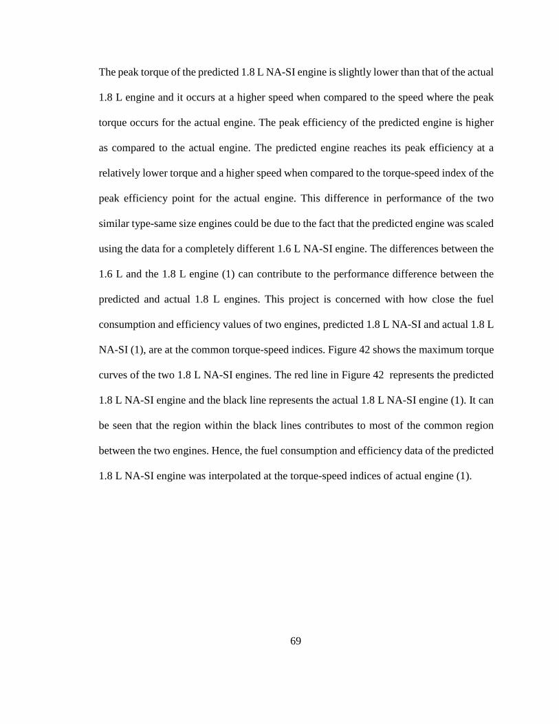
The peak torque of the predicted 1.8 L NA-SI engine is slightly lower than that of the actual

1.8 L engine and it occurs at a higher speed when compared to the speed where the peak

torque occurs for the actual engine. The peak efficiency of the predicted engine is higher

as compared to the actual engine. The predicted engine reaches its peak efficiency at a

relatively lower torque and a higher speed when compared to the torque-speed index of the

peak efficiency point for the actual engine. This difference in performance of the two

similar type-same size engines could be due to the fact that the predicted engine was scaled

using the data for a completely different 1.6 L NA-SI engine. The differences between the

1.6 L and the 1.8 L engine (1) can contribute to the performance difference between the

predicted and actual 1.8 L engines. This project is concerned with how close the fuel

consumption and efficiency values of two engines, predicted 1.8 L NA-SI and actual 1.8 L

NA-SI (1), are at the common torque-speed indices. Figure 42 shows the maximum torque

curves of the two 1.8 L NA-SI engines. The red line in Figure 42 represents the predicted

1.8 L NA-SI engine and the black line represents the actual 1.8 L NA-SI engine (1). It can

be seen that the region within the black lines contributes to most of the common region

between the two engines. Hence, the fuel consumption and efficiency data of the predicted

1.8 L NA-SI engine was interpolated at the torque-speed indices of actual engine (1).

69

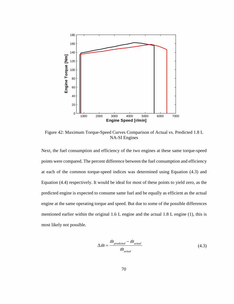
Figure 42: Maximum Torque-Speed Curves Comparison of Actual vs. Predicted 1.8 L NA-SI Engines

Next, the fuel consumption and efficiency of the two engines at these same torque-speed

points were compared. The percent difference between the fuel consumption and efficiency

at each of the common torque-speed indices was determined using Equation (4.3) and

Equation (4.4) respectively. It would be ideal for most of these points to yield zero, as the

predicted engine is expected to consume same fuel and be equally as efficient as the actual

engine at the same operating torque and speed. But due to some of the possible differences

mentioned earlier within the original 1.6 L engine and the actual 1.8 L engine (1), this is

most likely not possible.

−∆ =

predicted actual

actual

m mm

m (4.3)

1000 2000 3000 4000 5000 6000 70000

20

40

60

80

100

120

140

160

180

Engine Speed [r/min]

Eng

ine

Torq

ue [N

m]

70

η ηη

η−

∆ = predicted actual

actual (4.4)

Figure 43 and Figure 44 represent the error between the fuel consumption and efficiency

of the two similar type-same size engine. The contours in Figure 39 and Figure 40 represent

how much error occurs at the respective torque and speed, while the histograms in the

figures represent the how many points (y-axis) fall into each interval of the error (x-axis).

Table 10 shows the mean and standard deviation of all the fuel consumption and efficiency

error points. Looking at the both the contours in Figure 43 (b) and Figure 44 (b), it can be

noticed that the very high errors (up to 67% for efficiency and up to 65% for fuel

consumption) occurs in the low torque and high speed regions. As mentioned earlier,

because a vehicle rarely would operate in this low torque-high speed region, high error in

this region of the map is not of a concern. Data shown in Table 10 represents that the means

of both the fuel consumption and efficiency errors are less than 9 percent but, the standard

deviation are on the higher side of 17 and 20 percent respectively.

Finally, a comparison between the fuel consumption and efficiency error data,

represented in 4.2.1 and 4.2.2 of actual vs. actual and actual vs. predicted engines’

comparison is done. To contrast the difference the histograms of the fuel consumption and

efficiency error data for both the comparisons done in this section are placed side by side

as represented in Figure 45. On the left side of Figure 45 (a & c), the histograms for engine

efficiency error and fuel consumption error obtained from predicted vs. actual engines’

comparison are shown and the histograms for the same parameters for the actual vs. actual

71

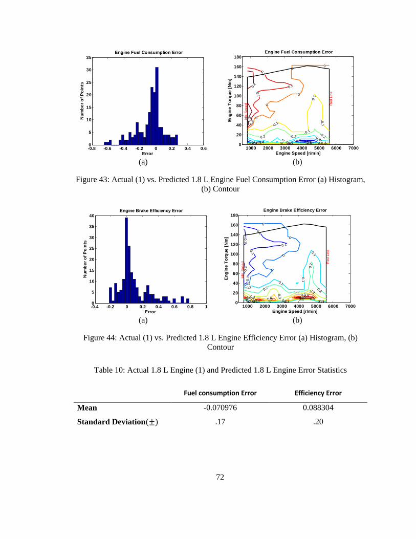
(a) (b)

Figure 43: Actual (1) vs. Predicted 1.8 L Engine Fuel Consumption Error (a) Histogram, (b) Contour

(a) (b)

Figure 44: Actual (1) vs. Predicted 1.8 L Engine Efficiency Error (a) Histogram, (b) Contour

Table 10: Actual 1.8 L Engine (1) and Predicted 1.8 L Engine Error Statistics

Fuel consumption Error Efficiency Error

Mean -0.070976 0.088304

Standard Deviation(±) .17 .20

-0.8 -0.6 -0.4 -0.2 0 0.2 0.4 0.60

5

10

15

20

25

30

35Engine Fuel Consumption Error

Error

Num

ber o

f Poi

nts

1000 2000 3000 4000 5000 6000 70000

20

40

60

80

100

120

140

160

180

Idle

Spe

ed Red

Lin

e

-0.6-0.5-0.4 -0.4 -0.4

-0.4-0.3

-0.3-0.3 -0.3-0

.3

-0.2 -0.2-0.2

-0.2 -0.2

-0.1

-0.1

-0.1

-0.1

-0.1 -0 1

0

0

0

0

0

0 0 0

0.1

0.1

0.1

0.1

0.2

0.2

Engine Speed [r/min]

Eng

ine

Torq

ue [N

m]

Engine Fuel Consumption Error

-0.4 -0.2 0 0.2 0.4 0.6 0.8 10

5

10

15

20

25

30

35

40Engine Brake Efficiency Error

Error

Num

ber o

f Poi

nts

1000 2000 3000 4000 5000 6000 70000

20

40

60

80

100

120

140

160

180

Idle

Spe

ed Red

Lin

e

-0.2

-0.2

-0.1

-0.1

-0.1

-0.1

0

0

0

0

00.1

0.1

0.1

0.1

0 1 0 1 0.1

0.20.2

0.2

0.2

0.2 0.2 0.20.3

0.3

0.3

0.3

0.3 0.30.4 0.4

0.4 0.40.4

0.5 0.5 0.50.5

0.50.6

0.60.7

Engine Speed [r/min]

Eng

ine

Torq

ue [N

m]

Engine Brake Efficiency Error

72

engines’ comparison are on the right side (b & d). Table 11 represents the means and

standard deviations of both the fuel consumption and efficiency errors of both the

comparisons.

Looking at Figure 45 it can be seen that the errors (fuel consumption and efficiency)

obtained when the two actual engines were compared (b & d) are much more dispersed

about the zero error as compared to the errors obtained from the predicted vs. actual

engines’ comparison. This could be the reason that the means of the errors for actual vs.

actual comparison are lower than the means of the errors obtained from predicted vs. actual

comparison, as can be seen in Table 11. The standard deviation for the errors obtained from

prediction vs. actual comparison are lower for the fuel consumption and same for the

efficiency as compared to the standard deviation for the errors obtained from actual vs.

actual comparison. The mean and the standard deviation values of the error obtained from

the 2 comparisons show that the engine scaling tool is scaling the engines accurately and

can be used by the EcoCAR 3 team.

More simply put, the scaled version of the 1.6 L to 1.8 L engine is just as similar as

one 1.8 L engine is to another 1.8 L engine. Given the goals of the high-level vehicle

design tasks that this scaling tools will be used for, this accuracy is sufficient.

73

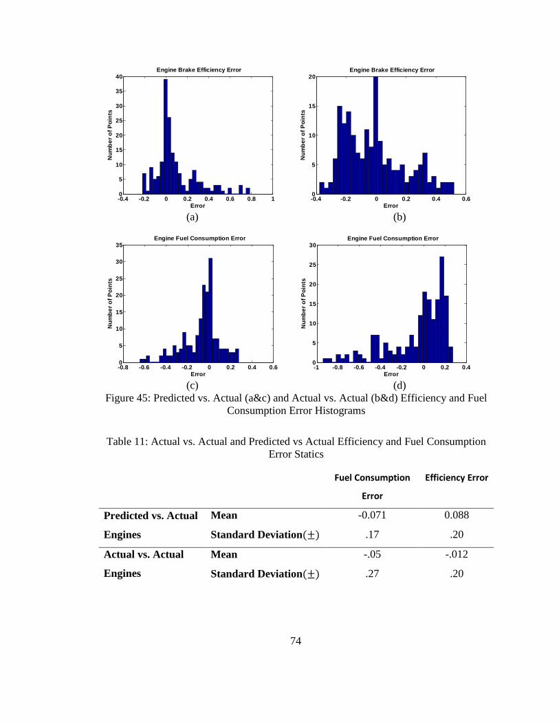
(a) (b)

(c) (d)

Figure 45: Predicted vs. Actual (a&c) and Actual vs. Actual (b&d) Efficiency and Fuel Consumption Error Histograms

Table 11: Actual vs. Actual and Predicted vs Actual Efficiency and Fuel Consumption Error Statics

Fuel Consumption

Error

Efficiency Error

Predicted vs. Actual

Engines

Mean -0.071 0.088

Standard Deviation(±) .17 .20

Actual vs. Actual

Engines

Mean -.05 -.012

Standard Deviation(±) .27 .20

-0.4 -0.2 0 0.2 0.4 0.6 0.8 10

5

10

15

20

25

30

35

40Engine Brake Efficiency Error

Error

Num

ber o

f Poi

nts

-0.4 -0.2 0 0.2 0.4 0.60

5

10

15

20Engine Brake Efficiency Error

Error

Num

ber o

f Poi

nts

-0.8 -0.6 -0.4 -0.2 0 0.2 0.4 0.60

5

10

15

20

25

30

35Engine Fuel Consumption Error

Error

Num

ber o

f Poi

nts

-1 -0.8 -0.6 -0.4 -0.2 0 0.2 0.40

5

10

15

20

25

30Engine Fuel Consumption Error

Error

Num

ber o

f Poi

nts

74

4.3 Electric Machine Scaling

Unlike the engine scaling validation, to validate the EM scaling method adopted by

this project, only one comparisons is done. This is due to the reason that not enough data

was available to make the second comparison. The energy conversion data for existing

brushless PM motors available to the EcoCAR 2 team through Parker-Hannifin were: the

GVM210-100, which has a rotor of 100 mm stack length and the GVM210-150, which has

a rotor of 150mm stack length, both with a common radius rotor. The rotor volumes for

GVM210-100 and GVM210-150 are 1.4 L and 2.1 L respectively. This project scaled

another 2.1 L PM motor, from the 1.4 L rotor EM, using the tool developed in this project

as shown in Chapter 2:. The scaled 2.1 L rotor EM had the same physical parameters (rotor

volume and rotor radius) as the already existing brushless PM motor with a 2.1 rotor. The

predicted energy conversion efficiency data of the scaled EM with 2.1 L rotor is compared

against the energy conversion efficiency data of the actual PM motor with 2.1 L rotor, both

of which have the same physical parameters. Figure 36 shows all the data available and the

dotted boxes around the boxes show the comparisons done for this project.

Figure 46: Electric Machine Comparisons

75

4.3.1 Actual vs. Predicted EM Comparison

The predicted energy conversion efficiency data of the scaled EM with a 2.1 L EM

is compared against the energy conversion efficiency data of the actual EM with a 2.1 L

EM, and the side by side comparison can be seen in Figure 47. On the left side of Figure

47 (a), energy conversion efficiency of the actual EM is shown and the efficiency map for

the predicted EM is on the right side (b). Table 12 lists the two EM’s peak torque, peak

power output, peak efficiency, and stall continuous torque values as well as the indexed

torque and speed where those points occur on their respective maps. Looking at Table 12

and Figure 47 it can be seen that the predicted motor with 2.1 L rotor has a lower power

output, higher peak, and stall continuous torque but the same peak speed when compared

to the actual EM with 2.1 L rotor. The same peak speed for both the EMs could be due to

the same radius of the predicted and the actual motors’ rotors. Peak energy conversion

efficiencies of the two EMs is about the same but the corresponding torque-speed indices

where it occurs are different for both the EMs. The actual EM reaches its peak efficiency

at a higher torque and speed as compared to the predicted EM. The base speed, the speed

that separates the constant torque and constant power region, of the two EM’s is also

different. The predicted motor has a base speed value of 4000 RPM compared to 5000

RPM of the actual EM. This difference in performance of the two similar type-same size

EMs could be due to the differences between the original actual EM (brushless PM motor

with a 1.4 L rotor), used to scale the predicted 2.1 L EM, and the actual EM with the 2.1 L

rotor. Physical differences between the two motors or in the inverter calibration explain

76

these differences. This project is concerned with how close the energy conversion

efficiency values of these two EMs are at the common torque-speed indices.

(a) (b)

Figure 47: Actual (a) vs. Predicted (b) EM’s Energy Conversion Efficiency Comparison

Table 12: Actual vs. Predicted PM Motors with 2.1 L Rotors’ Parameter Comparison

Actual brushless PM motor

(2.1 L rotor) Predicted brushless PM motor

(2.1 L rotor)

Torque (Nm) Speed (RPM) Torque (Nm)

Speed (RPM)

Peak Torque (Nm) 260 260 0-5000 270 270 0-4000

Peak Power Output (kW) 135 260-156 5000-8000 115 270-143 4000-

8000

Peak efficiency 94.1 86 7650 95 90.5 4345.7

Peak Stall Continuous Torque (Nm) 152 152 - 152 145.4 -

Figure 48 shows the maximum torque curves of the two brushless PM motors each with a

2.1 L rotor. The red line in Figure 42 represents the predicted EM’s maximum torque and

the black line represents the actual EM’s maximum torque. It can be seen that the region

within the red lines contributes to most of the common region between the two EM’s

0 2000 4000 6000 8000-400

-300

-200

-100

0

100

200

300

4000.

7

0.7

0.7

0.7

0.7

0.7

0.75

0.75

0.75

0.75

0.75

0.75

0.8

0.8

0.8

0.8

0.8

0.8

0.8

0.85

0.85

0.85

0.85

0.85

0.85

0.85

0.850.85 0.85

0.87

0.87

0.87

0.87

0.87

0.87

0.87

0.870.870.87 0.87

0.89

0.89

0.89

0.89

0.890.89

0.89

0.890.890.89 0.89 0.89

0.91

0.91

0.91

0.91

0.91 0.91

0.91

0.910.910.910.91 0.91 0.91

0.920.92

0.92

0.92 0.92 0.92

0.920.920.92

0.920.92

0.92

0.930.93

0.93

0.93 0.93 0.93

0.930.930.93

0.930.93

0.93

0.94

0.94

0.94

0.94 0.94

0.940.940.94

0.940.94

0.95

0.95

Speed [RPM]

Torq

ue [N

m]

Efficiency

0 2000 4000 6000 8000-300

-200

-100

0

100

200

300

0.7

0.7

0.7

0.7

0.7

0.7

0.7

0.75

0.750.75

0.75

0.75

0.75

0.75

0.8

0.8

0.8

0.8

0.8

0.8

0.8

0.8

0.850.85

0.85

0.850.85

0.85

0.85

0.850.850.85

0.870.87

0.87

0.87

0.87

0.87

0.87

0.870.870.87 0.87

0.890.89

0.89

0.89

0.89

0.89

0.89

0.890.890.89 0.89 0.89

0.910.91

0.91

0.91 0.91 0.91

0.910.910.91

0.91

0.91 0.91

0.920.92

0.92

0.92 0.92 0.92

0.920.920.92

0.92

0.92 0.92

0.93

0.93

0.93 0.93 0.93

0.930.930.93

0.930.93

0.94

0.94

Speed [RPM]

Torq

ue [N

m]

Efficiency

77

operating regions. Hence, the energy conversion efficiency data of the actual PM motor

with a 2.1 L rotor was interpolated at the torque-speed indices of the predicted EM.

Figure 48: Maximum Torque-Speed Curves Comparison of Actual vs. Predicted EMs with 2.1 L Rotors

Moving further, the energy conversion efficiency of the two EMs at these same

torque-speed points were compared. The percent difference between efficiency at each of

the common torque-speed indices was determined using Equation (4.5). It would be ideal

for most of these points to yield zero, as the predicted EM is expected be equally as efficient

as the actual EM, with the same physical parameters, at the same operating torque and

speed points. But due to some of the possible differences mentioned earlier between the

original EM with a 1.4 L rotor and the actual EM with 2.1 L rotor this is most likely not

possible.

0 1000 2000 3000 4000 5000 6000 7000 8000 9000-300

-200

-100

0

100

200

300

Speed [RPM]

Torq

ue [N

m]

78

η ηη

η−

∆ = predicted actual

actual (4.5)

Figure 49: Actual vs. Predicted EMs with 2.1 L EMs’ Fuel Efficiency Error (a) Histogram, (b) Contour

Figure 49 represents the percent difference between the efficiencies of the two (predicted

vs. actual) similar type-same size EMs. The contour in and Figure 49 (b) represent how

much percent-error occurs at the respective torque and speed, while the histograms in the

figure represent the how many points (y-axis) fall into each interval of the error (x-axis).

Table 13 shows the mean and standard deviation of all the efficiency error points seen in

Figure 49.

Table 13: Actual and Predicted EMs with 2.1 L Rotor Efficiency Error Statistics

Efficiency Error

Mean -.0484

Standard Deviation(±) .08

-0.8 -0.6 -0.4 -0.2 0 0.20

500

1000

1500

2000

2500Efficiency Error

Error

Num

ber o

f Poi

nts

0 2000 4000 6000 8000-300

-200

-100

0

100

200

300

-025

-0.2

5

-0.2

5

-0.25

-024

-0.2

4

-0.2

4

-0.24

-023

-0.2

3

-0.2

3

-0.23

-022

-0.2

2

-0.2

2

-0.22

-021

-0.2

1

-0.2

1

-0.21

-02

-0.2

-0.2

-0.2

-019

-0.1

9

-0.1

9

-0.19

-018

-0.1

8

-0.1

8

-0.18

-017

-0.1

7

-0.1

7

-0.17

-0.16

-0.1

6

-0.1

6

-0.16

-015

-0.1

5-0

.15

-0.15-0

14

-0.1

4-0

.14

-0.14-0

13

-0.1

3

-0.13

-0.1

3

-0.13

-0.13

-012

-0.1

2

-0.12

-0.1

2

-0.12

-0.12

-011

-0.1

1

-0.11

-0.1

1

-0.11

-0.11

-01

-0.1

-0.1

-0.1

-0.1

-0.1

009 -0.

09

-0.09

-0.0

9 -0.09

-0.09

008 -0.

08

-0.08

-0.0

8

-0.08

-0.08

007 -0.07

-0.07

-0.0

7

-0.07

-0.070

06

-0.06

-0.06

-0.0

6

-0.06

-0.060

05

-0.05

-0.0

5

-0.0

5

-0.05

-0.05

004

-0.0

4

-0.0

4

-0.04

-0.04

-0.04

-0.04

003

-0.0

3

-0.03

-0.03

-0.03

-0.03

-0.03

-0.03

002

-0.0

2

-0.02

-0.02

-0.02

-0.02

-0.02

-0.02

-0.02-0.02

001

-0.0

1

-0.01

-0.01

-0.01

-0.01

-0.01

-0.01

-0.01

-0.01

00

0

0

0

0

0

Speed [RPM]

Torq

ue [N

m]

Efficiency Error

79

Looking at the contour in Figure 49 (b), it can be noticed that low error occurs in the entire

map. The highest error noticed are at the low speeds (under 400 RPM) and of the highest

one being 17%. The error in this region of the map is not of a huge concern. Data shown

in Table 13 represents that the mean efficiency errors are less than 5 percent and the

standard deviation are 8 percent, which are statistically acceptable numbers. The mean and

the standard deviation values obtain shows that the EM scaling tool is scaling the EMs

accurately and can be used by the EcoCAR 3 team.

80

CHAPTER 5: CONCLUSION AND FUTURE WORK

The tools developed and validated for this project are capable of scaling engine and

electric machine data with the desired accuracy. The engine scaling tool scales the fuel

consumption data of a baseline engine to a different size engine, belonging to the same

category. The EM scaling tool scales the power (consumption and output) of a baseline

EM to a different size EM, belonging to the same category. Currently, the EcoCAR 3 team

is using both the tools for HEV architecture design for the Chevrolet Camaro, which the

team will be receiving in December 2015.

For further advancement of the tool, developed in this project, different engines and

electric machines with various technologies can be scaled and the accuracy for scaling the

different technologies will have to be examined. If the tools scale the performance aspects

of the engine and EM with different engine and EM technology respectively, in an

acceptable fashion, a library of engines and EMs could be further developed. This would

help the EcoCAR team test any energy converter of different technology and size within

EcoSIM and help the team understand how performance of an HEV varies with more

degrees of freedom.

81

CHAPTER 6: BIBLIOGRAPHY

1. Global Industry Analysts, I. Stringent Regulations for Curbing Greenhouse Gas

Emissions Drives Demand for Emission Control Catalysts. 2013; Available

from: http://www.prweb.com/releases/emission_control_catalyst/autocatalysts_m

arket/prweb11342846.htm.

2. Quality, E.O.o.T.a.A., EPA and NHTSA Set Standards to Reduce Greenhouse

Gases and Improve Fuel Economy for Model Years 2017-2025 Cars and Light

Trucks. August 2012(EPA-420-F-12-05): p. 1-10.

3. Research consortium of the Indiana, M.a.O.L.M.I.O., Driving Workforce Change:

Regional Impact and Implications of Auto Industry Transformation to a Green

Economy. 2013. p. 7-12.

4. Bovee, K., Design of the Architecture and Supervisory Control Strategy for a

Parallel-Series Plug-in

Hybrid Electric Vehicle, in Mechanical Engineering. 2012, The Ohio State University.

5. Chan, C.C., The State of the Art of Electric, Hybrid, and Fuel Cell Vehicles.

Proceedings of the IEEE, 2007. 95(4): p. 704-718.

6. Chan, C.C., A. Bouscayrol, and K. Chen, Electric, Hybrid, and Fuel-Cell

Vehicles: Architectures and Modeling. Vehicular Technology, IEEE Transactions

on, 2010. 59(2): p. 589-598.

7. Tate, E.D., M.O. Harpster, and P.J. Savagian, The Electrification of the

Automobile: From Conventional Hybrid, to Plug-in Hybrids, to Extended-Range

82

Electric Vehicles. SAE Int. J. Passeng. Cars - Electron. Electr. Syst., 2008. 1(1):

p. 156-166.

8. Zeman, J., et al., Modeling and Optimization of Plug-In Hybrid Electric Vehicle

Fuel Economy. 2012, SAE International.

9. Ehsani, M., G. Yimin, and J.M. Miller, Hybrid Electric Vehicles: Architecture

and Motor Drives. Proceedings of the IEEE, 2007. 95(4): p. 719-728.

10. Energy, U.S.D.o., U.S. HEV Sales by Model. April 2014: Alternative Fuels Data

Center.

11. Rizzoni, G., L. Guzzella, and B.M. Baumann, Unified modeling of hybrid electric

vehicle drivetrains. Mechatronics, IEEE/ASME Transactions on, 1999. 4(3): p.

246-257.

12. Heywood, J.B., Internal Combustion Engine Fundamentals. 1988, New York:

McGraw-Hill.

13. Woldring, D., T. Landenfeld, and M.J. Christie, DI Boost: Application of a High

Performance Gasoline Direct Injection Concept. 2007, SAE International.

14. Ricardo, A Study of Potential Effectiveness of Carbon Dioxide Reducing Vehicle

Technologies. 2008, U.S. Environmental Protection Agency.

15. Zeraoulia, M., M.E.H. Benbouzid, and D. Diallo, Electric Motor Drive Selection

Issues for HEV Propulsion Systems: A Comparative Study. Vehicular

Technology, IEEE Transactions on, 2006. 55(6): p. 1756-1764.

83

16. Momoh, O.D. and M.O. Omoigui. An overview of hybrid electric vehicle

technology. in Vehicle Power and Propulsion Conference, 2009. VPPC '09. IEEE.

2009.

17. Rahman, Z., M. Ehsani, and K.L. Butler, An Investigation of Electric Motor Drive

Characteristics for EV and HEV Propulsion Systems. 2000, SAE International.

18. Gao, D.W., C. Mi, and A. Emadi, Modeling and Simulation of Electric and

Hybrid Vehicles. Proceedings of the IEEE, 2007. 95(4): p. 729-745.

19. D. Assanis, G.D., R. Fellini, Z. Filipi, J. Liedtke, N. Michelena, and D.R. P.

Papalambros, D. Rosenbaum, A. Sales, M. Sasena, An Optimization Approach to

Hybrid Electric Propulsion

System Design. 1999.

20. Pries, J. and H. Hofmann, Magnetic and thermal scaling of electric machines.

International Journal of Vehicle Design, 2013. 61(1): p. 219-232.

84