09/02/2014 02:4 PM48-56_Wilm_Duff y_TP_Sept_2014_Final.indd 48

48 WILMOTT magazine

Modeling Volatility and Valuing Derivatives Under AnchoringPaul WilmottWilmott Associates, e-mail: paul@wilmott.com Alan L. LewisOptionCity.netDaniel J. Duff yDataism Education BV

AbstractWe develop a complete-markets model with volatility smiles, tractability, and intui-tive appeal as an anchoring or habit-formation model. Like traditional stochastic volatility models, it is invariant to a multiplicative scaling of the stock price levels. The anchoring effect is that the volatility depends on the relative value of the current stock price compared to its past history, with an exponential weighting.

Keywordsanchoring, behavioral finance, skew, volatility modeling

1 In troductionIn the subject of quantitative finance there are few clues as to how to model the vari-ables from first principles; how shares, commodities, interest rates, credit risk, and other instruments ought to behave. In the language of stochastic calculus this means that the functional forms of the drift and volatility in any stochastic differential equa-tion are almost arbitrary. Take interest rates for example, what we want of our model is that rates should stay positive (even this is open to question), and neither blow up nor get absorbed. Apart from that, virtually any interest rate model is acceptable. Thus, there is rarely any peg on which to hang our modeling hat, so to speak.

There is one exception to this observation. And that exception is that there is a class of financial instruments that ought to be modeled by a process that has certain lognormal or geometric characteristics. With shares and exchange rates we are not concerned about the price level per se, rather we care about its new level compared with a previous one. It is the return that matters. Clearly this is different from inter-est rates or credit risk, where the level makes a big difference to our perception of the instrument. If we have $1000 to spend, we are not concerned about the share price, we just have to buy more or fewer shares.

This suggests that a good model for a share price S would be the stochastic differ-ential equation dS = mSdt + sSdX with s being perhaps time dependent, but certainly

not being stock-price dependent. This model has the scaling property that if we multiply S by any constant then dS is increased by the same factor and so the return dS/S remains unchanged. Immediately this means that models such as CEV and local volatility, where the volatility depends on the level of S, are, according to our one modeling clue, unacceptable.

Rather than simply dismiss models such as CEV and local volatility, we should ask why they are popular. The answer is that they can give theoretical option values that more closely match those option values seen in the market, in particular in terms of implied volatility skews and smiles. Whether these skews and smiles ought to be an output of a theoretical model, via a process such as calibration, is open to question (Wilmott, 2009). Nevertheless it is common experience, regardless of option values and purely in terms of the behavior of a stock, that if a stock falls significantly from a previous high then its volatility does seem to increase. And this does point at a vola-tility that depends on the stock level S.

Is there any way that we can reconcile these two apparently conflicting require-ments? Can we have a volatility that depends on S in a model that still has our scaling requirement? The answer is yes.1

1.1 AnchoringAcc ording to Wikipedia, anchoring is a cognitive bias that describes the common human tendency to rely too heavily on one trait or piece of information when mak-ing decisions. In the present context we use the word to refer to the natural tendency to compare the current level of a stock to some historical level or average. Of course, we may be misusing the word since there may be no bias at all, such a tendency might be perfectly rational. Yet it does fly in the face of almost all quantitative models of financial instruments.

In models of financial instruments it is extremely common, almost universal in fact, that information from the past is given less weight than ‘information’ from the future via option values, and implied volatilities. Note the use of inverted com-mas around the second ‘information.’ Obviously no one has a crystal ball. But there seems to be a preference for using quantitative numbers that anticipate what might happen in the future rather than learning from the past. These models even have a Copyright © 2014 by Paul Wilmott, Alan L. Lewis, and Daniel J. Duffy

09/02/2014 02:4 PM48-56_Wilm_Duff y_TP_Sept_2014_Final.indd 49

^

TECHNICAL PAPER

WILMOTT magazine 49

There may possibly be a minimum of s(x) if mid-values of x are thought of as being more stable than extreme values. (And this in turn may be seen in a resulting theoretical smile.)

We shall do most of the analytical development for general s(x) and then use a simple sigmoidal function when we discuss explicit examples.

2.4 Qualitative observation on share pri ces generallyFigure 1 shows two lines, one being the logarithm of Standard and Poor’s 500 index (SPX) from 1950 until March 2012, detrended, and the second being the inverse of the index, also detrended and shifted vertically. Essentially the latter is just the mirror image of the former. If we were dealing with simple, lognormal random walks then the choppy (that is Brownian Motion) nature of these two lines would be qualitatively similar. But there is one aspect of the real financial time series that is different from its mirror image: the artificial data, the mirror image, has peaks and troughs like a sea wave, the peaks being pointy and the troughs being rounded. With the real data this picture is upside down. The real data has pointed troughs and rounded crests. This is suggestive of higher volatility for lower relative share prices; relative since we have detrended the series in this picture. Again, this is consistent with our model.

3 Option valuation equationSince dA= 𝜆(S −A) dt (4)

the equation governing the value of anything but strongly path-dependent options is obviously2

Vt +12𝜎2

( SA

)S2VSS + rSVS − rV + 𝜆(S −A)VA = 0. (5)

This will have the usual final condition, at time t = T the expiration, representing the payoff. The direction of convection makes boundary conditions in A unnecessary.

4 Observations on xBy examining the sto chastic differential equation for x in isolation we can tell a great deal about the behavior of this model, and get some clues as to how to approach the determination of a functional form for s and for determining a value for l.

mathematical name, Markov. Yet share prices are governed by human actions and emotions (perhaps not at the millisecond time scale!) and those humans do draw on the past for clues to the future.

2 The modelW e are going to work with a model that has a memory. Let us introduce a new vari-able, A, representing averaging or, in the language of behavioral finance, anchoring (to an historical level) (see Tversky and Kahneman, 1974):

A = 𝜆∫t

∞e−𝜆(t−𝜏 )S(𝜏 ) d𝜏 . (1)

Note that this is just about the simplest memory function that has tractable properties.We now work with a volatility function s(x), a function to be determined, where

𝜉 = SA. (2)

Of course, if you multiply S everywhere by a constant then the variable x is unchanged. Thus the model has our scaling requirement.

Our model is thus

dS = 𝜇S dt+ 𝜎(𝜉 )S dX. (3)

Such a volatility function can be made consistent with the previously mentioned observation that volatility increases when prices are low, but crucially this means low relative to some historical average, not simply low in an absolute sense since that would be contrary to our scaling requirement.

Note this is not the only memory function that has the required property; anything of the form

f(∫

t

−∞g(S(t)S(𝜏 )

, t, 𝜏)

d𝜏)

would also be acceptable, but a general functional would be just too cumbersome for practical use.

We now explain the parameters in equations (1), (2), and (3).

2.1 mIn principle, we can similarly model m as a functional. This could give extremely rich dynamics to the S process. However, provided the standard technical requirements are met this is irrelevant for the valuation of derivatives, since our model is clearly complete and so allows dynamic hedging and thus risk-neutral valuation. When we come to determine the parameters in our model from historical time series (not  calibration), we will see whether the simplest m being a constant is sufficient to represent the statistics of the underlying.

2.2 lThe parameter l is a measure of the extent of memory, the larger it is the shorter the span of memory. We would guess that in the financial markets (relevant) human memory would be measured in months or a small number of years, not in weeks or decades. And by ‘memory’ here we really mean that part of a time series that is deemed relevant to the stock’s current performance, that is allows for ‘forgiveness’ as it were.

2.3 sFor a simple stock we would expect the sigma function to be larger for small values of x than for large values of x. (And this may result in a theoretical negative skew.) The function s(x), being a power of x, might be appealing since it mimics the CEV model (although ours is more sensible, having the desirable scaling property). We will discuss this case later, where we will see that it results in undesirable properties for x.

Figure 1: The time series for detrended log SPX from 1950 until March 2012.

09/02/2014 02:4 PM48-56_Wilm_Duff y_TP_Sept_2014_Final.indd 50

50 WILMOTT magazine

From Equations (1), (2), and (3) we have

d𝜉 = (𝜇 + 𝜆 − 𝜆𝜉 ) 𝜉 dt+ 𝜎(𝜉 )𝜉 dX.

We shall find it very useful to work with the Fokker–Planck Equation to relate the density function for x to the volatility function s(x). In the steady state (assuming it exists) we can relate these via the ordinary differential equation

12d2

d𝜉 2(𝜎(𝜉 )2𝜉 2P∞(𝜉 )

)= d

d𝜉(D(𝜉 )𝜉P∞(𝜉 )

), (6)

with P∞(x) being the steady-state distribution and D(x) = m + l – lx. Given any two out of the three functions s(x), m, and P∞(x), we can use this equation to determine the third. That is, assuming the model is correct.

From historical data for S, and hence for A, assuming that we know l, we can determine both s(x) and P∞(x). (The former by differencing the x time series as explained in Chapter 36 of Wilmott, 2006 and the latter by looking at the distribution of the time series data, as explained in the same chapter. These ideas were first intro-duced in Apabhai et al., 1995.) And since we are assuming m to be a constant, again easily determined from the time series if it assumed constant, Equation (6) can be used to check whether the model is internally consistent and robust.

5 Determining s(x) from the time seriesAs already mentioned, w e take daily prices for the Standard and Poor’s 500 index from 1950 until March 2012. First we estimate m, assuming it to be constant. This is not done in a particularly sophisticated way, just treating the asset price as the con-stant volatility model. It is found to be 0.0835. Next we wish to analyze the data for x. Choose a l that seems plausible – we shall shortly be performing an optimization that properly determines its value – and calculate a time series for A, using Equation (4) and a starting guess for A. Thus we have a time series for x. See Figure 2.

Difference this to get a time series dx, which is virtually equivalent to a time series for s(x)x dX since the time between data points is so small. From this we can estimate the function s(x) as explained in Wilmott (2006). The results are shown in Figure 3. (Note that this shows the s(x) after the (still to be described) optimization has been done, so in effect this is our model.)

This already shows the realistic, and expected, behavior in which the volatility is large for smaller x. Because we wish to manipulate this function we need to first fit a relatively simple function to it. We chose the sigmoidal function

a + b − a1 + e−c(ln (𝜉)−d)

.

The reason for this choice is the behavior for small and large x, where it asymptotes to two different volatility values. Figure 4 shows the original data and the fitted curve. (Again, this fitted curve is the one that is optimal as discussed shortly.)

6 Determining P¥(x) from the time seriesBy finding the probability density fu nction for the data in Figure 1, we find the func-tion P∞(x). See Figure 5. However, from equation (6) we have a relationship between the s(x) we have just found and the P∞(x) we have also just found. So we could for example take the found s(x) and use it to determine P∞(x). By integrating (6) we have

P∞(𝜉 ) =1

𝜉 2𝜎2exp

(2∫

𝜉𝜇 + 𝜆 − 𝜆s

s𝜎(s)2ds +C

). (7)

0.6

0.8

1

1.2

1.4

1.6

0

0.2

0.4

4/12/1949 12/27/20147/24/19982/18/19829/15/1965

S/I

Figure 2: The time series for x, SPX from 1950 until March 2012.

0.3

0.4

0.5

0.6

0.7

0.8

0

0.1

0.2

0 0.5 1 1.5 2ξ

sigmasigma (from dX)

Figure 3: s(x) from time series data.

0.4

0.5

0.6

0.7

0.8

0

0.1

0.2

0.3

0 0.5 1 1.5 2ξ

sigma

sigma (from dX)

Sigmoidal function

Figure 4: A sigmoidal function fitted to the data.

2

3

4

5

6

From empirical data

0

1

0

ξ

21.6 1.81.41.210.6 0.80.40.2

Probability Density Function, steady state

Figure 5: The steady-state PDF for x from time series data.

09/02/2014 02:4 PM48-56_Wilm_Duff y_TP_Sept_2014_Final.indd 51

^

TECHNICAL PAPER

WILMOTT magazine 51

This can be done numerically. The constant of integration C is chosen to ensure that the integral of the PDF over zero to infinity is one.3

Let us recap. We have picked a plausible value for l, which is by no means necessarily correct. This gives us a time series for x and hence a (fitted sigmoidal) function for s(x) and a steady-state PDF. The latter two are also related via equa-tion (7). There are five parameters in our model, l and four (a, b, c, d) for the sig-moidal s(x) function. We also have the parameter m estimated directly from the S time series.

7 The optimizationWe choose l and a, b, c, d to minimize a combined, weighted error by finding t he best fits for both:

1. the sigmoidal function to the empirical s function and 2. the steady-state PDF obtained from integrating the sigmoidal function to the

empirical mean and standard deviation of the steady-state distribution.

The results of the best-fit sigmoidal function have already been shown in Figure 4. The best-fit steady-state PDF is shown in Figure 6.

The best-fit parameters are

a = 0.60, b = 0.12, c = 10.82, d = −0.27 and 𝜆 = 0.90.

The last of these confirms a typical memory of the order of 1 year, as anticipated.

7.1 A note on the goodness of fitWe can fit the s function as accurately as we like, by choosing suitab ly flexible func-tions with sufficient degrees of freedom. But from that function follows the steady-state distribution P∞. There is no guarantee that this distribution should be anywhere near matching the empirically calculated distribution given that we have allowed no freedom whatsoever in the parameter m. Had we given ourselves the freedom to choose m to be a function of x or something even more general, then such a good fit would probably have been possible. But this was not guaranteed with the simple choice of m as a constant, and especially not with m being the constant given directly by the time series data. Considering this, the match of the two functions to the data is remarkable.

As a test of the robustness of the model we input different values for m and per-formed the same optimization. The fits were in no case anywhere near as impressive as when we used the historical value for m.

8 Numerical results for option valuesWe report results from two numerical solvers for the option valuation P DE. Both use Mathematica’s NDSolve.4 The state space for (S, A) is the (unbounded) positive first quadrant. For the first solver, we map this to the unit square (X, Y ) using the trans-formations X = S/(S + S0) and Y = A/(A + A0), where (S0, A0) are the initial ‘hot spot’ values. With that, let V(S,A,t) = Ke–rt h(X,Y,t), where t = T – t and K is the option strike price. Then equation (5) becomes ht = AhXX + BhX + ChY, with new (variable) PDE coefficients that are straightforward to develop. As noted earlier, boundary con-ditions are unnecessary at Y = 0 and Y = 1. Even if you are not a Mathematica user, our solver call for a put option should be fairly readable. It simply repeats the PDE, sets the initial/boundary conditions, and then specifies the method:

NDSolve[{D[h[X,Y,t],t] == A[X,Y] D[h[X,Y,t],{X,2}]+ B[X,Y] D[h[X,Y,t],X] + C[X,Y] D[h[X,Y,t],Y],h[X,Y,0] == Max[1-(S0/K)X/(1-X),0],h[Xmin,Y,t] == 1,h[Xmax,Y,t] == 0}, h, {X,Xmin,Xmax},{Y,Ymin,Ymax},{t,T,T},Method->{"MethodOfLines","SpatialDiscretization"->{"TensorProductGrid","Coordinates"->{xgrid,ygrid}}}]

The (X, Y ) spatial grid here is a uniform discretization in both directions: {i/N, j/N}, (i,j = 1,2,…, N–1), N an integer. Table 1 shows results on the implied volatility surface for various strikes with S0 = A0 = 100. The associated put option values and parameter set are found in Table 2. Note that the parameter set is different from the earlier example. The results are based on spatial grids of size 250 × 250, except for T = 100, which uses a mesh of size 200 × 200. Entries for T = 0 come from a separate theoretical analysis of the model’s asymptotics, as discussed below.

As a second test of the numerical results we discuss how to approximate the solution of the PDE (5) using the finite difference method (FDM) and subsequent

Table 1: Anchoring model: Black–Scholes implied volatility (%)

T K=60 K=80 K=100 K=120 K=1400 29.46 21.17 17.13 15.99 15.610.25 29.03 21.15 17.18 16.07 15.761 27.78 21.07 17.50 16.29 15.783 25.68 20.91 18.15 16.85 16.2210 24.04 21.62 19.92 18.77 17.97100 25.60 25.16 24.82 24.54 24.31

2

3

4

5

6

From empirical data

Probability Density Function, steady state

From differential equation

0

1

ξ

0 21.6 1.81.41.210.6 0.80.40.2

Figure 6: Best fit integrated steady-state PDF and empirical PDF.

Table 2: European-style option prices for Table 1 (p=put, c=call)

T K=60 K=80 K=100 K=120 K=1400.25 p 0.0004298 0.04264 2.832 18.593 38.296

c 40.731 21.017 4.049 0.0540 0.000039771 p 0.1700 0.8486 4.681 16.280 33.551

c 43.039 24.674 9.463 2.019 0.24603 p 0.9670 2.379 6.035 13.695 25.444

c 49.169 33.315 19.706 10.099 4.58310 p 1.928 3.534 5.988 9.558 14.397

c 65.171 54.524 44.725 36.043 28.629100 p 0.05594 0.08064 0.1073 0.1358 0.1658

c 99.609 99.485 99.363 99.242 99.123

Parameter set: a = 0.6, b = 0.15, c = 10, d = –0.3, r = 0.049, l = 0.5.

09/02/2014 02:4 PM48-56_Wilm_Duff y_TP_Sept_2014_Final.indd 52

52 WILMOTT magazine

implementation in C++. The PDE (5) is defined on the positive quarter-plane in S and A. In order to reduce it to a problem on a bounded domain, we can choose between the popular domain truncation and domain transformation techniques. We choose the latter approach, as already introduced in this section. We then transform equation (5) in the variables (S, A) to a convection–diffusion–reaction PDE in the variables (X, Y). In other words, we solve a transformed PDE on the unit square. In order to specify the full problem we define an initial condition (in this case the pay-off function) and boundary conditions. For the X (transformed underlying) vari-able we prescribe well-known boundary conditions for call and put options while no boundary conditions are needed for the transformed anchoring variable Y, as already mentioned.

In order to approximate the solution of the transformed PDE we have chosen to use the Alternating Direction Explicit (ADE) method (for the original source see Saul’yev, 1964 and for applications to computational finance see Duffy, 2009). There are two main ADE variants: first, the original Saul’yev scheme that is unconditionally stable and explicit and second, the Barakat–Clark (1966) scheme that is also uncon-ditionally stable and explicit but more accurate than the Saul’yev scheme. The main advantages of the ADE method are: it is fast, easy to program, and can be applied to a wide range of linear and nonlinear time-dependent PDEs (some examples are discussed in Pealat and Duffy, 2011, and Duffy and Germani, 2013). When applied to the problems in the current work we found excellent agreement between the results produced by ADE and those produced by Mathematica. We note that ADE uses a constant mesh size in time while NDSolve uses adaptive time-stepping.

We discuss the accuracy and performance of the Saul’yev scheme, in particular as applied to put option pricing and results in Table 2. This scheme has a truncation error and we note the presence of the inconsistent term

(Δth

)2

that affects accuracy, where Δt is the step-size in time and h is the step-size in space. We can thus take a large number of steps in order to reproduce the results in Table 2. In general, we can get two-digit accuracy behind the decimal point using 200 mesh points in each direction, for example. We can improve the accuracy by using the Barakat–Clark scheme that has a truncation error O(Δt2,h2) (note that there is no inconsistent term in this case). This scheme is discussed in Duffy (2009).

In order to compute the implied volatility values in Table 1 we use the Black–Scholes formula for calls and puts using the option values that we found using ADE. There are many methods to solve this nonlinear equation and in this case we used the fixed-point method in combination with Aitken’s delta-squared process to accelerate convergence. It is worth noting that the fixed-point method converges for any ini-tial guess because the corresponding iteration function is a contraction (Haaser and Sullivan, 1991). This is in contrast to the Newton–Raphson and bisection methods (for example), where it can sometimes be an issue to find good starting values for these iterative methods.

Finally, the ADE method is very efficient and does not need matrix solvers. In fact, most of the computational overhead lies in computing the sigmoidal function that we introduced in Section 5. This involves calling the exponential and logarithm functions, which are computationally expensive. We can then consider faster approximations to these functions or pre-computing lookup tables of the sigmoidal function. For an introduction to the finite difference method in finance, see Duffy (2006).

9 Dimensional reduc tion: pricing by Fourier transform

We introduce an alternative which reduces the PDE problem from two spatial fac-tors to one factor. Apart from its application to general time numerics, we need this development for our discussion of model asymptotics.

Consider general bivariate stochastic volatility models of the form

dS = (r − q)S dt + ��(y)S dW(1)

dy= b(y)dt + a(y)dW(2) ,

where dW(1) dW(2) = r(y)dt. For example, the Heston model and many others fit, with ��(y) =

√y , so that y is the variance rate. Our anchoring model fits with y = x = S/A,

s(y) = s(x), and r = 1, a degeneracy which is not a problem. Note that s(·) is a general function, while s(·) is the sigmoidal function. For simplicity, assume y is positive.

In traditional stochastic volatility models, for example (Heston, etc.), St transfor-mations do not affect yt, and one has scaling: invariance under St → kSt. Under the anchoring model, you need to transform the entire historical series: {St} → {kSt}. This is translational invariance for {xt} = {log St}. Under both types of scaling one has this key property: the marginal characteristic function Φ = E

[eiz(xt−x0 )|x0, y0] is condi-

tionally independent of x0, the conditioning being on y0.5 Thus, Φ = Φ (t, y0, z). This leads to the Fourier pricing formula for call options:

C(T , S0, y0;K) = S0 e−qT −Ke−rT ∫ℑz∈(0,1)

e−izmH (T, y0, z)z2 − iz

dz2𝜋

. (8)

Here, m ≡ log{S0e–qt/Ke–rt} is a natural measure of ‘moneyness’ and H(T, y0, z) ≡ eiz(r–q)T Φ (T, y0, –z). The integral notation means: integrate along a line parallel to the real z-axis, such that the imaginary part ℑz ∈ (0, 1). We had some discretion about where to integrate. We chose ℑz ∈ (0, 1) because that condition coincides with a strip of analyticity of the integrand whenever the process has both a bounded norm and a bounded expected stock price.6 It has been shown in Lewis (2000) that H(t, y, z) is a solution to the PDE problem

H𝜏= 1

2a2(y)Hyy + [b(y) − iz𝜌(y)�� (y)a(y)]Hy − c(z)��2 (y)H , (9)

where c(z) = (z2 – iz)/2. The solution we want has the initial condition H(0, y; z) =1. For our anchoring model (and many others), no boundary conditions are needed at y = 0 or y = ∞. For anchoring, H = H (t, x; z) and (9) becomes

H𝜏 =12𝜎2(𝜉 ) 𝜉 2H𝜉𝜉 + [(𝜆 + r− 𝜆 𝜉 )− iz𝜎2 (𝜉 )] 𝜉H𝜉 − c(z)𝜎2 (𝜉 )H . (10)

Figure 7: Anchoring model implied volatility vs. strike and maturity. The strikes range from 60 to 140, and the times range from 0 to 3 years. The numerical method uses equation (8) with a numerical PDE solver to obtain the integrand.

09/02/2014 02:4 PM48-56_Wilm_Duff y_TP_Sept_2014_Final.indd 53

^

TECHNICAL PAPER

WILMOTT magazine 53

As promised, we have achieved a dimensional reduction – at the expense of requiring complex numbers and an integration. The recipe here: write a one-dimensional solv-er for (10) and feed the solutions to (8), integrating along z = i/2 + u, u Î (0, ∞). This Fourier method is used to produce the implied volatility surface shown in Figure 7.

One check: consider the case where the sigmoidal function is degenerate, so that 𝜎2(𝜉 ) = 𝜎2

0 , a constant. Then, the solution to (10), subject to H(0, x; z) = 1, is H (𝜏 ,𝜉 ;z) = e−c(z)𝜎20 𝜏 . Note that this has no x-dependence. As shown in Appendix 2.1 of Lewis (2000), and as expected, (8) then yields the Black–Scholes formula with volatility s0.

Finally note that, unlike ‘traditional’ stochastic volatility models, the interest rate r appears in the ‘volatility’ SDE and consequently in the fundamental PDE (10). This has the consequence that the BS implied volatility takes on an additional dependence on r that cannot be absorbed into the moneyness variable m above. This nuance is discussed further below.

10 Model asymptoticsSome natural questions are: how does the mo del behave for large and small l, recall-ing that l sets the time scale for which history matters? In addition: how does the implied volatility surface behave for large and small T, where T is the time to an option maturity? Asymptotics help clarify the mathematical behavior of the model, which generally requires a numerical solution. Asymptotics may help create rela-tively faster calibrations, using them (when appropriate) as a substitute for our PDE solvers.

10.1 The implied volatility smile as T → 0Option prices equal their payoff function at T = 0. What is interesting is that, for any diffusion model (like ours), there is a nontrivial limit as T → 0 for the Black–Scholes (BS) implied volatility, call it Σ. Recall the Black–Scholes formula for a call option on a non-dividend-paying stock:

cBS(T , S0,K, 𝜎) = S0Φ(d1) −Ke−rTΦ(d2), with well-known d1, 2. Consider any (time-homogeneous Markov) n-dimensional diffusion model for a call option price. The model has stochastic factors x = (S, Y) with x an n -vector and Y an (n – 1)-vector. (In our anchoring model, n = 2 and Y = A or, Y = x take your pick.) Let C(T, S0, Y0; K) denote that general model option price, at time t = 0, for option maturity T and strike K. Then, Σ is defined by equating the model price to the BS price:

C(T , S0,Y0;K) = cBS(T ,S0,K, Σ). (11)

Of course, for this to work, we must allow Σ = Σ (T, K, S0, Y0). Remarkably, the complicated nonlinear inversion associated with (11), in general diffusion models, admits an (asymptotic) expansion of the form

Σ = Σ(0) + TΣ(1) + T2Σ(2) + · · · , as T → 0. (12)

So, for the limiting expiration smile, we have Σ(0) (K, S0, Y0) in general and Σ(0) (K, S0, A0) for our particular model here. Notice that in Table 1, we show entries for T = 0. They were obtained from the following formula:

Σ(0)(K, S0,A0) =log S0∕K

∫ S0∕A0K∕A0

dxx𝜎(x)

, (13)

where we recall that s(x) is our sigmoidal function. At K = S0, an application of l’Hospital’s rule is implied, which yields the asymptotic at-the-money implied volatil-ity s (S0/A0). [For Tables 1 and 2, S0 = A0 and s(1) ≈ 0.171342.] If s(x) = s0, a constant,

then (3) (with m = r) is the Black–Scholes SDE. Reassuringly, in that case, (13) cor-rectly regenerates Σ(0) = s0.

Figure 8 shows a plot of the formula in (13) for the parameter set of Table 2. In the sigmoidal function, a = 0.60, which is the maximum ‘local’ volatility; this is also seen in the figure to be the maximum implied volatility, as one would expect. Similarly, b = 0.15 in the minimum local and implied volatility.

At-the-money relationship. In practice, as T grows small, liquidity in options becomes concentrated near-the-money. By taking successive K-derivatives of equa-tion (13), and then setting K = S0, one can derive the following at-the-money rela-tions. To this end, abbreviating Σ(K) ≡ Σ(0)(K, S0, A0) and with x0 = S0/A0, we find

Σ(S0) = 𝜎(𝜉0),

S0Σ′(S0) =12𝜉0 𝜎

′(𝜉0),

S20 Σ′′(S0) =

13𝜉 20 𝜎

′′(𝜉0) −32𝜉0𝜎

′(𝜉0) −76𝜉 20

[𝜎 ′(𝜉0)]2

𝜎(𝜉0).

Derivation. Briefly, here is how (13) is obtained. We start with call option values in general n-dimensional models:

C(T , S0,Y0;K) = e−rT ∫ max(ST −K, 0)q(T , S0,Y0;ST )dST ,

where q is the transition density for a particle starting at x0 = (S0, Y0) to arrive at ST with any value of YT. Now, the asymptotic smile is obtained by taking two K-derivatives of both sides of (11) and comparing them as T → 0. First suppose the underlying n-factor diffusion has variance–covariance matrix a(x) = {aij(x)}. Denote the inverse of this matrix by g(x), so g(x) = a–1(x).

First, two K derivatives of the right-hand-side. Since the BS formula is based on the lognormal density, one has

𝜕2cBS𝜕K2 (T , S0,K, Σ) ≈ exp

{−(logS0∕K)2

2 (Σ(0))2 T

}.

(14)

(Note: all “≈” denote leading behaviors as T → 0, up to ignorable factors.)Now the left-hand-side. From Breeden–Litzenberger’s (1978) relation and a clas-

sic argument due to Varadhan (1967):

𝜕2C𝜕K2 (T ,S0,Y0;K) = e−rT q(T , S0, Y0;K) ≈ exp

{−d2(S0 ,Y0;K)2T

}, (15)

20 40 60 80 100 120 140K

0.1

0.2

0.3

0.4

0.5

σimp(K)

Figure 8: Asymptotic T → 0 implied volatility vs. strike. The figure shows a plot of the formula in equation (13) for the parameter set of Table 2.

09/02/2014 02:4 PM48-56_Wilm_Duff y_TP_Sept_2014_Final.indd 54

54 WILMOTT magazine

whered2(S0, Y0;K) ≡ min

x(0)=(S0 ,Y0)x(1)=(K,free)

∫1

0gij (x(s)) x

i(s) xj (s) ds.

In the integral shown for d2, the ‘min’ is a functional minimization over all parame-terized path functions {x(s): 0 ≤ s ≤ 1} subject to the endpoint conditions shown. The scalers xi are simply the components of x, x i(s) = dxi/ds, and there is an implied sum-mation over repeated indices. With that notation, d(S0,Y0; K) has a fascinating inter-pretation. It is the minimum geodesic distance in the (S, Y ) space from (S0, Y0) to the (hyperplane) S = K. The geodesics are those found by treating g = a–1 as a metric and doing deterministic (that is, non-stochastic) path calculations. Comparing the right-hand sides of (14) and (15) yields a general result for the asymptotic smile:

Σ(0)(K, S0,Y0) =||||

log S0∕Kd(S0,Y0;K)

|||| . (16)

Thus it comes down to calculating geodesic distance functions d(x, A), where x is again an n -dimensional point and A is any set in the factor variable space that does not contain x. There are a variety of ways to do this. One of the most straightforward ways is to solve the Eikonal equation,7 namely

aij(x)𝜕d𝜕xi

𝜕d𝜕xj

= 1,

subject to the boundary condition that d(x, A) vanishes when x touches A. For example, start with n = 1 and local volatility evolutions dSt = ��(St)StdWt . A drift may be present, but it plays no role in the limiting smile, so we ignore it. Then, a(S) = ��(S)2S2 and d = d(S; K ). Thus the Eikonal problem is easy: solve S2��(S)2(dS)

2 = 1, subject to d(S = K ) = 0. This has the solution

d(S;K) = ∫S

K

duu ��(u)

. (17)

Now our problem is a two-factor problem, dSt = s(St/At)StdWt, but the second factor At has an SDE with a drift but no Brownian term. Given that degeneracy, one would guess that local volatility formula (17) applies with ��(S) = 𝜎(S∕A0) . We recall that s(·) is the sigmoidal function. That is,

d(S0,A0;K) = ∫S0

K

duu 𝜎(u∕A0)

= ∫S0∕A0

K∕A0

dxx𝜎(x)

.

Applying (16), this last relation yields our formula (13). Our guess can be justified by setting up the full problem in two-dimensional (S, x) space, which is governed by a bivariate SDE with two (perfectly correlated) Brownian noise terms. Then, one shows that the putative solution for the distance function (but written in terms of S and x) satisfies the corresponding two-dimensional Eikonal equation. It is tedious, but straightforward, and a good exercise for the ambitious reader.

Further reading. The geodesic connection is developed in Varadhan (1967). See Lewis (2007) for a more elaborate but heuristic derivation of (16) and further referenc-es. See also the chapter on ‘Advanced smile asymptotics’ in Lewis (2014, forthcoming).

10.2 The implied volatility smile as T → ¥ The method is to develop the large-T behavior of the Fourier solution representation (8) and especially the behavior of the ‘fundam ental transform’ H(T, x0;z) in this limit. This method was developed in detail in Lewis (2000), so we will be brief.

In a nutshell, in general models, the implied volatility surface flattens at large matu-rity T. The flattening is to a common value independent of the moneyness and initial factors. In our case, the initial factors are (S0, x0). One has to be careful about what is held fixed as T → ∞. The natural thing is to fix the moneyness m = log {S0e–qT/Ke–rT },

and that is assumed throughout our discussion.8 With that, one can develop the simple relation for the ultimate implied variance

Vimp∞ = lim

T→∞Vimp(T ,m, 𝜉0) = 8 Λ0(y∗). (18)

Then, 𝜎 imp∞ =

√Vimp

∞ . In (18), Λ0(y) is the principal (i.e., smallest) eigenvalue associated with the (negative of the) spatial differential operator of (10), fixing z = iy (0 < y < 1). This leads to the eigenvalue problem u0(𝜉 ) = Λ0 u0(𝜉 ) , suppressing the dependence on the fixed y. The function space for u0 is: smooth enough functions with certain boundary behaviors. Then, y* is a stationary point; i.e., Λ0(y*) is the larg-est of such principal eigenvalues along the line segment y ∈ (0,1). For the parameter set of Table 2, but with r = 0, Figure 9 shows Λ0(y) and the associated eigenfunction at y =y*, the maximum point.

From (18), and the parameter set of Table 2, except for various interest rates r, Table 3 shows computed values of 𝜎 imp

∞ . To check the results (see Tables 3 and 4), the full time-dependent problem has also been solved with T = 1000. This was done by using the Fourier transform method, solving (10) for H(T, x; z) in Mathematica with NDSolve. For the finite-T solver call, no boundary conditions were taken at x = 0 and a zero x-derivative was taken at a cutoff xmax= 2. One can see that the finite maturity results are consistent with asymptotic values.

If one carried out this same exercise in, say, the Heston (1993) stochastic volatility model, all the values in Table 3 for 𝜎 imp

∞ would be the same. This is because the ultimate implied volatility flattens to a value that depends on the parameters in the volatility process, which does not contain r. Here, as noted earlier, such r-dependence is present.

Figure 9: ‘Large T asymptotics’ is an eigenvalue problem. As explained in the text, the asymptotic implied volatility as T → ∞ is associated with an eigen-value problem Lu0(x) = Ù0u0 (x), where Ù0 = Ù0(y *). For the parameter set of Table 2, but with r = 0, the figure shows Ù0(y) and the associated eigenfunc-tion at y = y*, the maximum point.

0.3 0.4 0.5 0.6 0.7y

0.00500.00550.00600.00650.0070

Λ(y) u0(ξ )

1 2 3 4ξ

0.60.70.80.91.0

Table 3: Black–Scholes implied volatilities (%): large T and T → ∞

T r = 0 r = 0.02 r = 0.04 r = 0.06 r = 0.08 r = 0.101000 23.58 21.61 19.94 18.56 17.50 16.71∞ 23.61 21.68 20.00 18.62 17.54 16.74

Table 4: Option prices corresponding to the T = 1000 entry in Table 3

r = 0 r = 0.02 r = 0.04 r = 0.06 r = 0.08 r = 0.1099.981 99.937 99.838 99.664 99.434 99.176

Parameter set: a = 0.6, b = 0.15, c = 10, d = –0.3, l = 0.5. For each r, the strike was set to the forward at-the-money value: K = S0erT.

09/02/2014 02:4 PM48-56_Wilm_Duff y_TP_Sept_2014_Final.indd 55

^

TECHNICAL PAPER

WILMOTT magazine 55

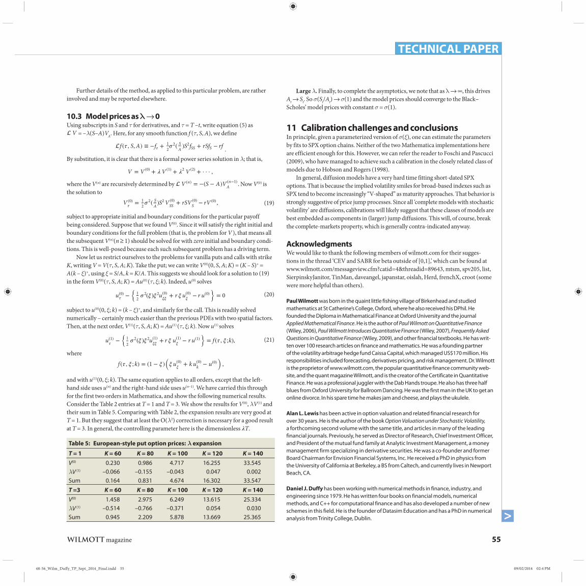
Table 5: European-style put option prices: l expansion

T = 1 K = 60 K = 80 K = 100 K = 120 K = 140V(0) 0.230 0.986 4.717 16.255 33.545lV (1) –0.066 –0.155 –0.043 0.047 0.002Sum 0.164 0.831 4.674 16.302 33.547

T =3 K = 60 K = 80 K = 100 K = 120 K = 140V(0) 1.458 2.975 6.249 13.615 25.334lV (1) –0.514 –0.766 –0.371 0.054 0.030Sum 0.945 2.209 5.878 13.669 25.365

Further details of the method, as applied to this particular problem, are rather involved and may be reported elsewhere.

10.3 Model prices as l → 0Using subscripts in S and t for derivatives, and t = T –t, write equation (5) as V  = –l(S–A)VA. Here, for any smooth function f (t, S, A), we define

f (𝜏 , S,A) ≡ −f𝜏 +12𝜎2( S

A)S2fSS + rSfS − rf .

By substitution, it is clear that there is a formal p ower series solution in l; that is,

V = V (0) + 𝜆V (1) + 𝜆2 V (2) + · · · ,

where the V(n) are recursively determined by V (n) = −(S − A)V (n−1)A . Now V(0) is

the solution to

V (0)𝜏

= 12𝜎2( S

A)S2V (0)

SS + rSV (0)S − rV (0) , (19)

subject to appropriate initial and boundary conditions for the particular payoff being considered. Suppose that we found V(0). Since it will satisfy the right initial and boundary conditions for the full problem (that is, the problem for V ), that means all the subsequent V(n)(n ≥ 1) should be solved for with zero initial and boundary condi-tions. This is well-posed because each such subsequent problem has a driving term.

Now let us restrict ourselves to the problems for vanilla puts and calls with strike K, writing V = V(t, S, A; K). Take the put; we can write V(0)(0, S, A; K) = (K – S)+ = A(k – x)+, using x = S/A, k = K/A. This suggests we should look for a solution to (19) in the form V(0)(t, S, A; K) = Au(0) (t, x; k). Indeed, u(0) solves

u(0)𝜏

−{

12𝜎2(𝜉 )𝜉 2u(0)

𝜉𝜉+ r 𝜉 u(0)

𝜉− r u(0)

}= 0 (20)

subject to u(0)(0, x; k) = (k – x)+, and similarly for the call. This is readily solved numerically – certainly much easier than the previous PDEs with two spatial factors. Then, at the next order, V(1)(t, S, A; K) = Au(1) (t, x; k). Now u(1) solves

u(1)𝜏

−{

12𝜎2(𝜉 )𝜉 2u(1)

𝜉𝜉+ r 𝜉 u(1)

𝜉− r u(1)

}= f (𝜏 , 𝜉 ;k), (21)

where

f (𝜏 , 𝜉 ;k) = (1 − 𝜉 )(𝜉 u(0)

𝜉+ k u(0)k − u(0)

),

and with u(1)(0, x; k). The same equation applies to all orders, except that the left-hand side uses u(n) and the right-hand side uses u(n–1). We have carried this through for the first two orders in Mathematica, and show the following numerical results. Consider the Table 2 entries at T = 1 and T = 3. We show the results for V(0), lV(1) and their sum in Table 5. Comparing with Table 2, the expansion results are very good at T = 1. But they suggest that at least the O(l2) correction is necessary for a good result at T = 3. In general, the controlling parameter here is the dimensionless �T.

Large l. Finally, to complete the asymptotics, we note that as l → ∞, this drives At → St. So s(St/At) → s(1) and the model prices should converge to the Black–Scholes’ model prices with constant s = s(1).

11 Calibration challenges and conclusionsIn principle, given a parameterized version of s(x), one can estimate the parameters by fits to SPX option chains. Neither of the two Mathematica implementations here are efficient enough for this. However , we can refer the reader to Foschi and Pascucci (2009), who have managed to achieve such a calibration in the closely related class of models due to Hobson and Rogers (1998).

In general, diffusion models have a very hard time fitting short-dated SPX options. That is because the implied volatility smiles for broad-based indexes such as SPX tend to become increasingly “V-shaped” as maturity approaches. That behavior is strongly suggestive of price jump processes. Since all ‘complete models with stochastic volatility’ are diffusions, calibrations will likely suggest that these classes of models are best embedded as components in (larger) jump diffusions. This will, of course, break the complete-markets property, which is generally contra-indicated anyway.

AcknowledgmentsWe would like to thank the following members of wilmott.com for their sugges-tions in the thread ‘CEV and SABR for beta outside of [0,1],’ which can be found at www.wilmott.com/messageview.cfm?catid=4&threadid=89643, mtsm, spv205, list, SierpinskyJanitor, TinMan, daveangel, japanstar, oislah, Herd, frenchX, croot (some were more helpful than others).

Paul Wilmott was born in the quaint little fishing village of Birkenhead and studied mathematics at St Catherine’s College, Oxford, where he also received his DPhil. He founded the Diploma in Mathematical Finance at Oxford University and the journal Applied Mathematical Finance. He is the author of Paul Wilmott on Quantitative Finance (Wiley, 2006), Paul Wilmott Introduces Quantitative Finance (Wiley, 2007), Frequently Asked Questions in Quantitative Finance (Wiley, 2009), and other financial textbooks. He has writ-ten over 100 research articles on finance and mathematics. He was a founding partner of the volatility arbitrage hedge fund Caissa Capital, which managed US$170 million. His responsibilities included forecasting, derivatives pricing, and risk management. Dr. Wilmott is the proprietor of www.wilmott.com, the popular quantitative finance community web-site, and the quant magazine Wilmott, and is the creator of the Certificate in Quantitative Finance. He was a professional juggler with the Dab Hands troupe. He also has three half blues from Oxford University for Ballroom Dancing. He was the first man in the UK to get an online divorce. In his spare time he makes jam and cheese, and plays the ukulele.

Alan L. Lewis has been active in option valuation and related financial research for over 30 years. He is the author of the book Option Valuation under Stochastic Volatility, a forthcoming second volume with the same title, and articles in many of the leading financial journals. Previously, he served as Director of Research, Chief Investment Officer, and President of the mutual fund family at Analytic Investment Management, a money management firm specializing in derivative securities. He was a co-founder and former Board Chairman for Envision Financial Systems, Inc. He received a PhD in physics from the University of California at Berkeley, a BS from Caltech, and currently lives in Newport Beach, CA.

Daniel J. Duffy has been working with numerical methods in finance, industry, and engineering since 1979. He has written four books on financial models, numerical methods, and C++ for computational finance and has also developed a number of new schemes in this field. He is the founder of Datasim Education and has a PhD in numerical analysis from Trinity College, Dublin.

09/02/2014 02:4 PM48-56_Wilm_Duff y_TP_Sept_2014_Final.indd 56

56 WILMOTT magazine

W

ENDNOTES 1. Our model is ‘complete with stochastic volatility,‘ in the sense of Hobson and Rogers (1998), and has similar features.2. We generally denote partial derivatives with a subscript, except where clarity suggests a more explicit notation.3. Not every choice for s(x) admits a stationary density, and a stationary density is not always needed. When s(0) < ∞, as is true for our sigmoidal parameterization, it is easy to see that

This leads to the x -stationarity condition: m + l > s(0)2/2. When s(0) < ∞, but the sta-tionary condition is violated, x -mass simply accumulates closer and closer to the natu-ral boundary x = 0 (similar to GBM). For some applications, say stocks with bankruptcy risk, unbounded s(·) may be desirable. Then, P∞(x) develops a Dirac mass at x = 0 and the existence of a stationary density in x becomes irrelevant. Finally, nothing much interesting happens for large x: for integrability there, it is sufficient that l > 0 and s(∞) < ∞. The latter condition is uncontroversial for most equities, as this is the regime of large S relative to history.4. The standard NDSolve algorithm is a ‘method of lines.’ Basically: apply a spatial PDE discretization, which converts the PDE into an ODE system. The latter is then solved by an adaptive time-stepping routine. There are many details.5. Such processes are sometimes termed Markov Additive Processes, or MAPs, in the applied probability literature.6. Those are very weak conditions. Our anchoring model, with a sigmoidal function bounded away from 0 and infinity, should be both norm-preserving and martingale-preserving – although we do not prove it.7. Sometimes called the Hamilton–Jacobi equation.8. Suppose S0 is fixed and we increase T. Note that fixing the moneyness is not the same as fixing the strike K, except when q = r.

REFERENCESApabhai, M.Z., Choe, K., Khennach, F., and Wilmott, P. (1995). Spot-on modelling. Risk magazine, December.

Barakat, H.Z. and Clark, J.A. (1966). On the solution of diffusion equations by numerical methods. Journal of Heat Transfer 88, 421–427.Breeden, D. and Litzenberger, R. (1978). Prices of state-contingent claims implicit in option prices. The Journal of Business 51(4), 621–651.Duffy, D.J. (2006). Finite Difference Methods in Financial Engineering. Wiley: Chichester, UK.Duffy, D.J. (2009). Unconditionally stable and second-order accurate explicit finite dif-ference schemes using domain transformations, Part I. One-factor equity problems. DOI: 10.2139/ssrn.1552926.Duffy, D.J. and Germani, A. (2013). C# for Financial Markets. Wiley: Chichester, UK.Foschi, P. and Pascucci, A. (2009). Calibration of a path-dependent volatility model: Empirical tests. Computational Statistics and Data Analysis 53(6), 2219–2235.Haaser, N.B. and Sullivan, J.A. (1991). Real Analysis. Dover Publications: New York.Heston, S. (1993). A closed-form solution for options with stochastic volatility with applications to bond and currency options. Review of Financial Studies 6(2), 327–343.Hobson, D.G. and Rogers, L.C.G. (1998). Complete models with stochastic volatility. Mathematical Finance 8(1), 27–48.Lewis, A. (2000). Option Valuation under Stochastic Volatility: With Mathematica Code. Finance Press: Newport Beach, CA.Lewis, A. (2007). Geometries and smile asymptotics for a class of stochastic volatility models. www.optioncity.net/publications.htm.Lewis, A. (2014). Option Valuation under Stochastic Volatility II: With Mathematica Code. Finance Press: Newport Beach, CA (forthcoming).Pealat, G. and Duffy, D.J. (2011). The alternating direction explicit (ADE) method for one factor problems. Wilmott magazine, July, 54–60.Saul’yev, V.K. (1964). Integration of Equations of Parabolic Type by the Method of Nets. Pergamon Press: Oxford, UK.Tversky, A. and Kahneman, D. (1974). Judgment under uncertainty: Heuristics and biases. Science 185, 1124–1130.Varadhan, S.R.S. (1967). On the behavior of the fundamental solution of the heat equation with variable coefficients; Diffusion processes in a small time interval. Communications on Pure and Applied Mathematics 20, 431–455; 659–685.Wilmott, P. (2006). Paul Wilmott on Quantitative Finance, 2nd edn. Wiley: Chichester, UK.Wilmott, P. (2009). Where quants go wrong: A dozen basic lessons in commonsense for quants and risk managers and the traders who rely on them. Wilmott Journal 1(1), 1–22.