Article

Localization Framework for Real-Time UAVAutonomous Landing: An On-Ground DeployedVisual Approach

Weiwei Kong 1,2, Tianjiang Hu 1,*, Daibing Zhang 1, Lincheng Shen 1 and Jianwei Zhang 3

1 College of Mechatronics and Automation, National University of Defense Technology,Changsha 410073, China; kongww.nudt@gmail.com (W.K.); swimsword@163.com (D.Z.);lcshen@nudt.edu.cn (L.S.)

2 Naval Academy of Armament, Beijing 100161, China3 Institute of Technical Aspects of Multimodal Systems (TAMS), Department of Computer Science,

University of Hamburg, 22527 Hamburg, Germany; zhang@informatik.uni-hamburg.de* Correspondence: t.j.hu@nudt.edu.cn

Academic Editors: Felipe Gonzalez Toro and Antonios TsourdosReceived: 31 March 2017; Accepted: 9 June 2017; Published: 19 June 2017

Abstract: One of the greatest challenges for fixed-wing unmanned aircraft vehicles (UAVs) is safelanding. Hereafter, an on-ground deployed visual approach is developed in this paper. This approachis definitely suitable for landing within the global navigation satellite system (GNSS)-deniedenvironments. As for applications, the deployed guidance system makes full use of the groundcomputing resource and feedbacks the aircraft’s real-time localization to its on-board autopilot.Under such circumstances, a separate long baseline stereo architecture is proposed to possessan extendable baseline and wide-angle field of view (FOV) against the traditional fixed baselineschemes. Furthermore, accuracy evaluation of the new type of architecture is conducted by theoreticalmodeling and computational analysis. Dataset-driven experimental results demonstrate the feasibilityand effectiveness of the developed approach.

Keywords: UAV; stereo vision; localization

1. Introduction

Over the past few decades, the application of unmanned aircraft has increased enormously in bothcivil and military scenarios. Although aerial robots have successfully been implemented in severalapplications, there are still new research directions related to them. Floreano [1] and Kumar et al. [2]outlined the opportunities and challenges of this developing field, from the model design to high-levelperception capability. All of these issues are concentrating on improving the degree of autonomy,which supports that UAVs continue to be used in novel and surprising ways. No matter whetherfixed-wing or rotor-way platforms, a standard fully-unmanned autonomous system (UAS) involvesperforms takeoffs, waypoint flight and landings. Among them, the landing maneuver is the mostdelicate and critical phase of UAV flights. Two technical reports [3] argued that nearly 70% of mishapsof Pioneer UAVs were encountered during the landing process caused by human factors. Therefore,a proper assist system is needed to enhance the reliability of the landing task. Generally, two maincapabilities of the system are required. The first one is localization and navigation of UAVs, and thesecond one is generating the appropriate guidance command to guide UAVs for a safe landing.

For manned aircraft, the traditional landing system uses a radio beam directed upward fromthe ground [4,5]. By measuring the angular deviation from the beam through onboard equipment,the pilot knows the perpendicular displacement of the aircraft in the vertical channel. For the azimuth

Sensors 2017, 17, 1437; doi:10.3390/s17061437 www.mdpi.com/journal/sensors

Sensors 2017, 17, 1437 2 of 17

information, additional equipment is required. However, due to the size, weight and power (SWaP)constraints, it is impossible to equip these instruments in UAV. Thanks to the GNSS technology, we haveseen many successful practical applications of autonomous UAVs in outdoor environments such astransportation, aerial photography and intelligent farming. Unfortunately, in some circumstances,such as urban or low altitude operations, the GNSS receiver antenna is prone to lose line-of-sightwith satellites, making GNSS unable to deliver high quality position information [6]. Therefore,autonomous landing in an unknown or global navigation satellite system (GNSS)-denied environmentis still an open problem.

The visual-based approach is an obvious way to achieve the autonomous landing by estimatingflight speed and distance to the landing area, in a moment-to-moment fashion. Generally, two types ofvisual methods can be considered. The first category is the vision-based onboard system, which hasbeen widely studied. The other is to guide the aircraft using a ground-based camera system. Once theaircraft is detected by the camera during the landing process, its characteristics, such as type, location,heading and velocity, can be derived by the guidance system. Based on this information, the UAVcould align itself carefully towards the landing area and adapt its velocity and acceleration to achievesafe landing. In summary, two key elements of the landing problem are detecting the UAV and itsmotion, calculating the location of the UAV relative to the landing field.

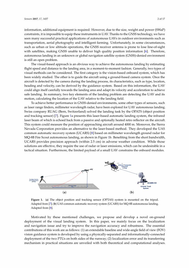
To achieve better performance in GNSS-denied environments, some other types of sensors, suchas laser range finders, millimeter wavelength radar, have been explored for UAV autonomous landing.Swiss company RUAG (Bern, Switzerland) solved the landing task by the OPATS (object positionand tracking sensor) [7]. Figure 1a presents this laser-based automatic landing system, the infraredlaser beam of which is echoed back from a passive and optionally heated retro reflector on the aircraft.This system could measure the position of approaching aircraft around 4000 m. Moreover, the SierraNevada Corporation provides an alternative to the laser-based method. They developed the UAScommon automatic recovery system (UCARS) [8] based on millimeter wavelength ground radar forMQ-8B Fire Scout autonomous landing, as shown in Figure 1b. Benefiting from the short bandwidth,UCARS provides precision approach (within 2.5 cm) in adverse weather condition. While thosesolutions are effective, they require the use of radar or laser emissions, which can be undesirable in atactical situation. Furthermore, the limited payload of a small UAV constrains the onboard modules.

The Object Positionand Tracking Sensor

(OPTAS)

Detection Range4 km

(a)

Ground Track System

UCARS-V2

Airborne TransponderSubsystem

(1.8 kg)

(b)

Figure 1. (a) The object position and tracking sensor (OPTAS) system is mounted on the tripod.Adapted from [7]; (b) UAS common automatic recovery system (UCARS) for MQ-8B autonomous landing.Adapted from [8].

Motivated by these mentioned challenges, we propose and develop a novel on-grounddeployment of the visual landing system. In this paper, we mainly focus on the localizationand navigation issue and try to improve the navigation accuracy and robustness. The essentialcontributions of this work are as follows: (1) an extendable baseline and wide-angle field of view (FOV)vision guidance system is developed by using a physically-separated and informationally-connecteddeployment of the two PTUs on both sides of the runway; (2) localization error and its transferringmechanism in practical situations are unveiled with both theoretical and computational analyses.

Sensors 2017, 17, 1437 3 of 17

In particular, the developed approach is experimentally validated with fair accuracy and betterperformance in timeliness, as well as practicality against the previous works.

The remainder of this paper is organized as follows. Section 2 briefly reviews the related works.In Section 3, the architecture of the on-ground deployed stereo system is proposed and designed.Section 4 conducts the accuracy evaluation, and its transferring mechanism is conducted throughtheoretical and computational analysis. Dataset-driven validation is followed in Section 5. Finally,concluding remarks are presented in Section 6.

2. Related Works

While several techniques have been applied for onboard vision-based control of UAVs, fewhave shown landing of a fixed-wing guiding by a ground-based system. In 2006, Wang [9] proposeda system using a step motor controlling a web camera to track and guide a micro-aircraft. This camerarotation platform expands the recognition area from 60 cm × 60 cm–140 cm × 140 cm, but the range ofthe recognition is only 1 m. This configuration cannot be used to determine the position of a fixed-wingin the field.

At Chiba University [10], a ground-based Bumblebee stereo vision system was used to calculatethe 3D position of a quadrotor at the altitude of 6 m. The Bumblebee has a 15.7-cm baseline with a66◦ horizontal field of view. The sensor was mounted on a tripod with the height of 45 cm, and thedrawback of this system is the limited baseline leading to a narrow field of view (FOV).

To increase the camera FOV, multi-camera systems are considered attractive. This kind of systemcould solve the common vision problems and track objects to compute their 3D locations. In addition,Martinez [11] introduced a trinocular on-ground system, which is composed of three or more camerasfor extracting key features of the UAV to obtain robust 3D position estimation. The lenses of theFireWire cameras are 3.4 mm and capture images of a 320× 240 size at 30 fps. They employed thecontinuously-adaptive mean shift (CamShift) algorithm to track the four cooperation markers withindependent color, which were distributed on the bottom of the helicopter. The precision of thissystem in the vertical and horizontal direction is around 5 cm and in depth estimation is 10 cm with a3-m recognition range. The maximum range for depth estimation is still not sufficient for fixed-wingUAV. Additionally, another drawback of the multi-camera system is the calibration process, whoseparameters are nontrivial to obtain.

A state-of-the-art study from Guan et al. [12] proposed a multi-camera network with laserrangefinders to estimate an aircraft’s motion. This system is composed of two sets of measurementunits that are installed on both sides of the runway. Each unit has three high-speed cameras withdifferent focal lengths and FOV to captures the target in the near-filed (20 m–100 m), middle-field(100 m–500 m) and far-field (500 m–1000 m), respectively. A series of field experiments shows thatthe RMS error of the distance is 1.32 m. Due to the configuration of the system, they have to apply aoctocopter UAV equipped with a prism to calibrate the whole measurement system.

Except the camera-based ground navigation system, the ultra-wide band (UWB) positioningnetwork is also discussed in the community. Kim and Choi [13] deployed the passive UWB anchors bythe runway, which listen for the UWB signals emitted from the UAV. The ground system computesthe position of the target based on the geometry of the UWB anchors and sends it back to the UAVthrough the aviation communication channel. There are a total of 240 anchor possible locations, asshown in Figure 2b, distributed at each side of the runway, and the longitudinal range is up to 300 mwith a positioning accuracy of 40 cm.

Sensors 2017, 17, 1437 4 of 17

C1C3

C5

C7 C2C4

C8

C6

LeftSystem

RightSystem

Processor

(a)

40

-40 40

0

5

10

15

Up(m)

Lateral(m)

Longitudinal(m)

-200

20

0-20-40 20

RunwayAnchor

Array

Anchor Array

Anchor Array

Anchor Array

(b)

Figure 2. (a) Architecture of the multi-camera network. (b) In the longitudinal direction, there are20 anchors separated by 3 m. In the vertical direction, the anchors are either located on the ground orat the 10-m height antennas. The red points show the 240 possible anchor locations.

Our group first developed the traditional stereo ground-based system with infrared cameras [14],while this system has limited detection distance. For short-baseline configuration, cameras weresetup on one PTU, and the system should be mounted on the center line of the runway. However,the short-baseline limits the maximum range for UAV depth estimation. To enhance the operatingcapability, we conducted the triangular geometry localization method for the PTU-based system [15].As shown in Figure 3, we fixed the cameras with separate PTUs on the both sides of the runway.Therefore, the landing aircraft can be locked by our system around 1 km. According to the previouswork, the localization accuracy largely depends on the aircraft detection precision in the cameraimage plane. Therefore, we implemented the Chan–Vese method [16] and the saliency-inspiredmethod [17] to detect and track the vehicle more accurately; however, these approaches are not suitablefor real-time requirements.

Radio Link

Right Vision Unit

Left Vision Unit

Pan/Tilt Angle and Image FrameBase Line

GroundStation

Pan/Tilt Angle and Image Frame

PTU Control

Command

PTU Control

Command

Router

Ground Stereo Vision System

UAV SystemIR Camera

VisibleLight

Camera

PTU

Desired Touchdown Point

3 ~ 7°

Figure 3. Architecture of the ground stereo vision system.

Sensors 2017, 17, 1437 5 of 17

For more information, we also reviewed various vision-based landing approaches performedon different platforms [18], and Gautam provides another general review of the autonomous landingtechniques for UAVs [19].

3. System Architecture and Deployment

In this section, we introduce the theoretical model for the ground-to-air visual system. We firstrecap the traditional stereo vision model, which has a limited baseline, restraining the detectiondistance. To enlarge the system working boundary, we setup the camera and other sensor modules onthe two separated PTUs and then calculate the target according to the image information and rotationangle from PTU. Each vision unit works independently and transfers the results of image processingand PTU status to the navigation computer, which calculates the estimated relative position of theUAV. The architecture of the ground stereo vision system is shown in Figure 3.

3.1. Fundamental Principles of Ground-Based Stereo Systems

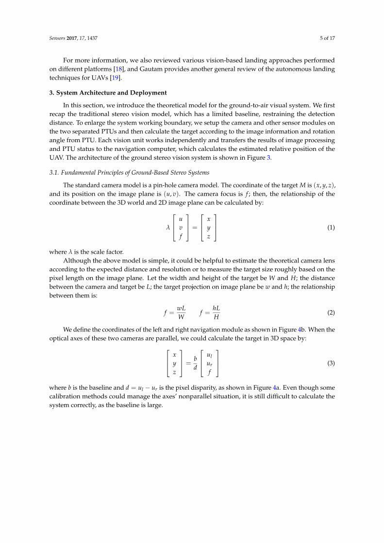
The standard camera model is a pin-hole camera model. The coordinate of the target M is (x, y, z),and its position on the image plane is (u, v). The camera focus is f ; then, the relationship of thecoordinate between the 3D world and 2D image plane can be calculated by:

λ

uvf

=

xyz

(1)

where λ is the scale factor.Although the above model is simple, it could be helpful to estimate the theoretical camera lens

according to the expected distance and resolution or to measure the target size roughly based on thepixel length on the image plane. Let the width and height of the target be W and H; the distancebetween the camera and target be L; the target projection on image plane be w and h; the relationshipbetween them is:

f =wLW

f =hLH

(2)

We define the coordinates of the left and right navigation module as shown in Figure 4b. When theoptical axes of these two cameras are parallel, we could calculate the target in 3D space by: x

yz

=bd

ulur

f

(3)

where b is the baseline and d = ul − ur is the pixel disparity, as shown in Figure 4a. Even though somecalibration methods could manage the axes’ nonparallel situation, it is still difficult to calculate thesystem correctly, as the baseline is large.

Sensors 2017, 17, 1437 6 of 17

𝒃𝒃

UAV

c ,O ci

,O ck

𝑓𝑓

lr

( ,0, )b f(0,0, )f

( , )l lu v ( , )r ru v

Left Image Plane Right Image Plane

Left CameraRight Camera

𝑓𝑓

)𝑴𝑴(𝒙𝒙,𝒚𝒚, 𝒛𝒛

(a)

𝑿𝑿

𝒁𝒁

𝑭𝑭𝒍𝒍 𝑭𝑭𝒓𝒓

𝒀𝒀

𝝍𝝍𝒍𝒍

𝝓𝝓𝒍𝒍

𝝍𝝍𝒓𝒓𝝓𝝓𝒓𝒓

𝑨𝑨

𝑵𝑵

𝑴𝑴

𝑭𝑭

𝑭𝑭𝒍𝒍𝒛𝒛

Left Vision Unit Right Vision Unit

𝑭𝑭𝒍𝒍𝒍𝒍

𝑭𝑭𝒍𝒍𝒚𝒚

𝑭𝑭𝒓𝒓𝒍𝒍

𝑭𝑭𝒓𝒓𝒚𝒚

𝑭𝑭𝒓𝒓𝒛𝒛

(b)

Figure 4. (a) Theoretical stereo vision model; (b) theoretical optical model. The target M is projected atthe center of the optical axis.

3.2. Separated Long Baseline Deployment

In order to detect the target at long distance, a large baseline, more than 5 m, is required.Benefiting the camera assembled on the PTU separately, we could switch the baseline freely accordingto the expected detection distance and target size.

In this paper, we assumed that the world coordinate system (X, Y, Z) is located on the origin ofthe left vision unit, the rotation center of the PTU. For the sake of simplicity, the camera is installed onthe PTU in the way that the axes of the camera frame are parallel to those of the PTU frame. The originsof these two frames are close. Therefore, it can be assumed that the camera frame coincides withthe body frame. Figure 4b reveals the theoretical model for visual measurement. After installingthe right camera system on the X-axis, the left and right optical center can be expressed as Ol andOr, respectively. Then, the baseline of the optical system is OlOr, whose distance is D. Consideringthe center of mass of the UAV as a point M, Ol M and Or M illustrate the connections between theeach optical center and the UAV. In addition, φl , φr, ψl , ψr denote the tilt and pan angle on both sides.Therefore, we define φl = 0, φr = 0, ψl = 0 and ψr = 0, as the PTU is set to the initial state, i.e., theoptical axis parallel to the runway; the measurement of the counterclockwise direction is positive.

Since the point M does not coincide with the principle point, which is the center of the image plane,the pixel deviation compensation in the longitudinal and horizontal direction should be considered.As shown in Figure 5, we calculate pixel deviation compensation on the left side by:

ψcl = arctan(u− u0)du

f

φcl = arctan(v− v0) cos ψcldv

f

(4)

where the optical point is o(uo, vo), du and dv are the pixel length of the u- and v-axis in image planeand f is the focus. The current PTU rotation angle can be directly obtained through the serial portsduring the experiments. Let φpl and ψpl be the left pan and tilt angle separately. Then, the total panand tilt angle on the left side can be detailed as:{

φl = φcl + φpl

ψl = ψcr + ψpr(5)

Sensors 2017, 17, 1437 7 of 17

𝒖𝒖

Image Plane

𝑓𝑓𝑥𝑥

𝒇𝒇𝒚𝒚

𝒇𝒇𝒛𝒛

𝐹𝐹

𝑴𝑴(𝒖𝒖,𝒗𝒗)

𝝍𝝍𝒄𝒄𝒄𝒄

𝜶𝜶𝑭𝑭𝑭𝑭𝑭𝑭/𝟐𝟐

𝝓𝝓𝒄𝒄𝒄𝒄 𝒄𝒄

𝒇𝒇

𝒘𝒘𝒖𝒖/𝟐𝟐

𝒘𝒘𝒗𝒗/𝟐𝟐

𝑢𝑢0, 𝑣𝑣0

𝒗𝒗

𝑴𝑴(𝒙𝒙,𝒚𝒚, 𝒛𝒛)

UAV

c,O ci

,O ck

,O cj

Figure 5. The geometry of one PTUwith respect to the optical center and the image plane.

For the other side, we could also calculate the angle in the same way.The world coordinates of point M is (xM, yM, zM) ∈ R3. Point N is the vertical projection of point

M on the XOY plane, and NA is perpendicular to the X-axis. If we define NA = h, the followingnavigation parameters can be obtained:

xM = h tan ψl =D tan ψl

tan ψl − tan ψr

yM = h =D

tan ψl − tan ψr

zM =h tan φlcos ψl

=D tan φl

cos ψl(tan ψl − tan ψr)

(6)

Furthermore, errors in the internal and external camera calibration parameters marginally affectsome of the estimates: the x-position and z-position, in particular.

4. Accuracy Evaluation of the On-Ground Stereo System

4.1. Theoretical Modeling

We are now in the position to analyze the error related to the PTU rotation angle. The discussionwas first presented in our previous works [15]. According to Equation (6), the partial derivatives ofeach equation with respect to the pan angle and the tilt angle are denoted in the following way,

∂xM∂ψl

=D tan ψr

cos2 ψl(tan ψl − tan ψr)2

∂xM∂ψr

=D tan ψl

cos2 ψr(tan ψl − tan ψr)2

(7)

Sensors 2017, 17, 1437 8 of 17

∂yM∂ψl

=D

cos2 ψl(tan ψl − tan ψr)2

∂yM∂ψr

=D

cos2 ψr(tan ψl − tan ψr)2

(8)

∂zM∂φl

=D

cos ψl cos2 φl(tan ψl − tan ψr)

∂zM∂ψl

=D tan φl(cos ψl + sin ψl tan ψr)

cos2 ψr(tan ψl − tan ψr)2

∂zM∂ψr

=D tan φl

cos ψl cos2 ψr(tan ψl − tan ψr)2

(9)

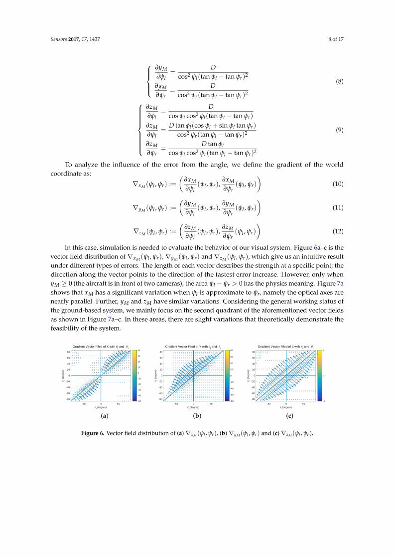
To analyze the influence of the error from the angle, we define the gradient of the worldcoordinate as:

∇xM (ψl , ψr) :=(

∂xM∂ψl

(ψl , ψr),∂xM∂ψr

(ψl , ψr)

)(10)

∇yM (ψl , ψr) :=(

∂yM∂ψl

(ψl , ψr),∂yM∂ψr

(ψl , ψr)

)(11)

∇zM (ψl , ψr) :=(

∂zM∂ψl

(ψl , ψr),∂zM∂ψr

(ψl , ψr)

)(12)

In this case, simulation is needed to evaluate the behavior of our visual system. Figure 6a–c is thevector field distribution of∇xM (ψl , ψr),∇yM (ψl , ψr) and∇zM (ψl , ψr), which give us an intuitive resultunder different types of errors. The length of each vector describes the strength at a specific point; thedirection along the vector points to the direction of the fastest error increase. However, only whenyM ≥ 0 (the aircraft is in front of two cameras), the area ψl − ψr > 0 has the physics meaning. Figure 7ashows that xM has a significant variation when ψl is approximate to ψr, namely the optical axes arenearly parallel. Further, yM and zM have similar variations. Considering the general working status ofthe ground-based system, we mainly focus on the second quadrant of the aforementioned vector fieldsas shown in Figure 7a–c. In these areas, there are slight variations that theoretically demonstrate thefeasibility of the system.

-50 0 503

l (degree)

-80

-60

-40

-20

0

20

40

60

80

3r (

degr

ee)

Gradient Vector Filed of X with 3l and 3

r

-50

-40

-30

-20

-10

0

10

20

30

40

(a)

-50 0 503

l (degree)

-80

-60

-40

-20

0

20

40

60

80

3r (

degr

ee)

Gradient Vector Filed of Y with 3l and 3

r

-80

-60

-40

-20

0

20

40

60

80

(b)

-50 0 503

l (degree)

-80

-60

-40

-20

0

20

40

60

80

3r (

degr

ee)

Gradient Vector Filed of Z with 3l and 3

r

-5

0

5

(c)

Figure 6. Vector field distribution of (a) ∇xM (ψl , ψr), (b) ∇yM (ψl , ψr) and (c) ∇zM (ψl , ψr).

Sensors 2017, 17, 1437 9 of 17

-35 -30 -25 -20 -15 -10 -53

l (degree)

5

10

15

20

25

30

35

3r (

degr

ee)

Gradient Vector Filed of X with 3l and 3

r in Second Quadrant

-9

-8

-7

-6

-5

-4

-3

-2

-1

(a)

-35 -30 -25 -20 -15 -10 -53

l (degree)

5

10

15

20

25

30

35

3r (

degr

ee)

Gradient Vector Filed of Z with 3l and 3

r in Second Quadrant

0.5

1

1.5

2

2.5

3

(b)

-35 -30 -25 -20 -15 -10 -53

l (degree)

5

10

15

20

25

30

35

3r (

degr

ee)

Gradient Vector Filed of X with 3l and 3

r in Second Quadrant

-9

-8

-7

-6

-5

-4

-3

-2

-1

(c)

-6040

-50

-40

30 0

-30Y

-20

Gradient of Y with 3l and 3

r in Second Quadrant

-10

3r (degree)

20

-10

3l (degree)

0

-2010 -30

0 -40

-55

-50

-45

-40

-35

-30

-25

-20

-15

-10

(d)

040

1

30 0

2Z

Gradient of Z with 3l and 3

r in Second Quadrant

-10

3

3r (degree)

20

3l (degree)

4

-2010 -30

0 -40

0.5

1

1.5

2

2.5

3

(e)

-1040

-8

-6

30 0

X

-4

Gradient of X with 3l and 3

r in Second Quadrant

-10

3r (degree)

-2

20

3l (degree)

0

-2010 -30

0 -40-9

-8

-7

-6

-5

-4

-3

-2

-1

(f)

Figure 7. (a–c) Vector field distribution of ∇xM (ψl , ψr), ∇yM (ψl , ψr), and ∇zM (ψl , ψr) in the secondquadrant; (d–f) gradient of X, Y, Z with θl and θr in the second quadrant.

4.2. Computational Analysis

In theory, Ol M and Or M should intersect perfectly at one point all of the time, as shown inFigure 4b. Due to the inevitable errors from PTU rotation and tracking algorithms, we estimate theintersecting point by combing the vertical line of two different planes in space.

(1) We set (xol , yol , zol) = (0, 0, 0), and (xor, yor, zor) = (D, 0, 0) is the optical center of each camera.Assuming that al 6= 0, bl 6= 0, cl 6= 0 and ar 6= 0, br 6= 0, cr 6= 0, we obtain the parametric equations oflines Ol M and Or M:

x− xolal

=y− yol

bl=

z− zolcl

= tl ,

x− xor

ar=

y− yor

br=

z− zor

cr= tr,

(13)

al = cos φl sin ψlbl = cos φl cos ψlcl = sin φl

ar = cos φr sin ψr

br = cos φr cos ψr

cr = sin φr

(14)

where tl , tr are the parameters for the line Ol M and Or M separately. Therefore, any point (x, y, z) oneach line is usually written parametrically as a function of tl and tr:

xl = altl + xolyl = bltl + yolzl = cltl + zol

xr = arlr + xor

yr = brtr + yor

zr = crtr + zor

(15)

(2) In our situation, Ol M and Or M are skew lines, such that these two lines are no parallel and donot intersect in 3D. Generally, the shortest distance between the two skew lines lies along the line that

Sensors 2017, 17, 1437 10 of 17

is perpendicular to both of them. By defining the intersection points of the shortest segment line foreach line by (xlp, ylp, zlp) and (xrp, yrp, zrp), we get the parametric equations:

xlp = altl + xolylp = bltl + yolzlp = cltl + zol

xrp = arlr + xor

yrp = brtr + yor

zrp = crtr + zor

(16)

(3) Knowing the position of the intersection points on each line, the distance is calculated by thesquare Euclidean norm:

J = ‖(xlp, ylp, zlp)− (xrp, yrp, zrp)‖22 (17)

(4) By deriving the function J, we achieved the minimum distance when ∂J∂tl

= 0 and ∂J∂tr

= 0.Then, the above functions derive the following equation:[

a2l + b2

l + c2l −(alar + blbr + clcr)

−(alar + blbr + clcr) a2l + b2

l + c2l

] [tltr

]

= (xol − xor)

[−alar

]+ (yol − yor)

[−blbr

]+ (zol − zor)

[−clcr

].

We could define the matrix on the left side as:

H =

[a2

l + b2l + c2

l −(alar + blbr + clcr)

−(alar + blbr + clcr) a2l + b2

l + c2l

](18)

Considering that there is a uniqueness vertical line, so det H 6= 0, and the position of the targetpoint Min the world coordinate is:xM

yMzM

= w

xlpylpzlp

+ (1− w)

xrp

yrp

zrp

, w ∈ [0, 1]. (19)

where w is weight, and the other parameters are:

xlp = al Dal(a2

l + b2l + c2

l )− ar(al ar + blbr + clcr)

(albr − bl ar)2 + (blcr − clbr)2 + (alcr − cl ar)2

ylp = bl Dal(a2

l + b2l + c2

l )− ar(al ar + blbr + clcr)

(albr − bl ar)2 + (blcr − clbr)2 + (alcr − cl ar)2

zlp = cl Dal(a2

l + b2l + c2

l )− ar(al ar + blbr + clcr)

(albr − bl ar)2 + (blcr − clbr)2 + (alcr − cl ar)2

(20)

and:

xrp = D

[ar

al(al ar + blbr + clcr)− ar(a2l + b2

l + c2l )

(albr − bl ar)2 + (blcr − clbr)2 + (alcr − cl ar)2 + 1

]

yrp = brDal(al ar + blbr + clcr)− ar(a2

l + b2l + c2

l )

(albr − bl ar)2 + (blcr − clbr)2 + (alcr − cl ar)2

zrp = crDal(al ar + blbr + clcr)− ar(a2

l + b2l + c2

l )

(albr − bl ar)2 + (blcr − clbr)2 + (alcr − cl ar)2

(21)

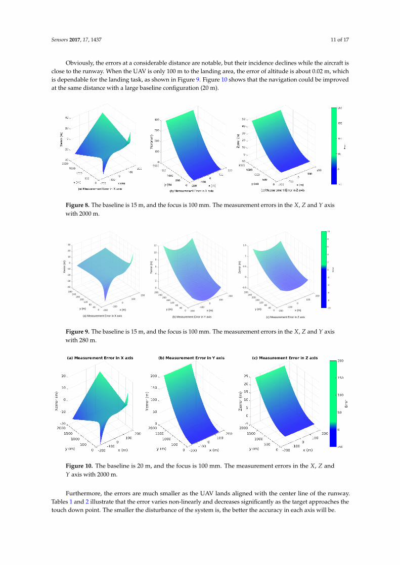
The angle between the UAV landing trajectory and the runway area is usually between 3◦ and7◦. By considering 1 mrad normal distributed disturbance (the accuracy of the PTU is 0.006◦), Figure 8illustrates measurement errors of xM, yM and zM in the case of different points (x, y) ∈ S, whereS = {(x, y)| − 50 ≤ x ≤ 50, 20 ≤ y ≤ 1000}.

Sensors 2017, 17, 1437 11 of 17

Obviously, the errors at a considerable distance are notable, but their incidence declines while the aircraft isclose to the runway. When the UAV is only 100 m to the landing area, the error of altitude is about 0.02 m, whichis dependable for the landing task, as shown in Figure 9. Figure 10 shows that the navigation could be improvedat the same distance with a large baseline configuration (20 m).

Figure 8. The baseline is 15 m, and the focus is 100 mm. The measurement errors in the X, Z and Y axiswith 2000 m.

-40

-30

280

-20

240

-10

200

0

Xer

ror

(m)

200

10

100

y (m)

160

20

x (m)

120

30

080

-100400 -200

(b) Measurement Error in Y axis

0

2

280

4

240 200

6

Yer

ror

(m)

200

8

100

y (m)

160

10

x (m)

120

12

080

-100400 -200

(c) Measurement Error in Z axis

-0.5

280

0

240 200

0.5

Zer

ror

(m)

200100

1

y (m)

160

x (m)

120

1.5

080

-100400 -200

-10

-8

-6

-4

-2

0

2

4

6

8

10

Err

or

(a) Measurement Error in X axis

Figure 9. The baseline is 15 m, and the focus is 100 mm. The measurement errors in the X, Z and Y axiswith 280 m.

Figure 10. The baseline is 20 m, and the focus is 100 mm. The measurement errors in the X, Z andY axis with 2000 m.

Furthermore, the errors are much smaller as the UAV lands aligned with the center line of the runway.Tables 1 and 2 illustrate that the error varies non-linearly and decreases significantly as the target approaches thetouch down point. The smaller the disturbance of the system is, the better the accuracy in each axis will be.

Sensors 2017, 17, 1437 12 of 17

Table 1. Errors when the center extraction of the aircraft with 1-pixel disturbance, f = 100 mm andD = 10 m.

Error (m)/Distance (m) 4000 3000 2000 1000 500 200 100 50

Xerror −1.44 −1.16 −0.63 −0.65 −0.25 −0.10 −0.05 −0.05Yerror 1141.92 692.31 333.44 195.65 23.82 3.92 1.00 0.25Zerror 133.42 82.62 39.24 22.70 2.43 0.28 0.03 −0.02

Table 2. Errors when the center extraction of the aircraft with 5-pixel disturbance, f = 100 mm andD = 10 m.

Error (m)/Distance (m) 4000 3000 2000 1000 500 200 100 50

Xerror −3.33 −3.00 −2.53 −2.14 −1.02 −0.46 −0.23 −0.13Yerror 2663.28 1800.31 1000.11 642.87 100.23 18.19 4.17 1.23Zerror 320.66 214.93 117.73 74.57 10.24 1.32 0.09 −0.07

Different from the traditional binocular vision system, the optical axes of each vision unit are not parallelduring the operation, and there is an initial offset between the camera optical center and the rotation axes ofPTU. Therefore, the traditional checkerboard pattern calibration method is not sufficient and convenient to obtainthe stereo system parameters for our large baseline system. To solve the calibration issue, we firstly chose theintrinsic camera model, which includes the principal point displacement, optical distortions, skew angle, etc.Each camera should be calibrated separately by the classical black-white chessboard method with the help of thecalibration module from OpenCV. Secondly, we setup the setting points with the help of the differential GlobalPositioning System (DGPS) module and calibrate the system based on the PTU rotation angle, coordinates and theground-truth position of the setting points.

4.3. Rotation Compensation

According to the above discussion, the 3D location estimation depends largely on the precision of the targetcenter position in the image plane. Our previous work [16,17,20] introduced saliency-inspired and the Chan–Vesemodel method to track the UAV during the landing progress. Both of these approaches predict and extract thecenter of the UAV position without considering the PTU rotation. However, in the practical situation, the PTUmight jump suddenly due to the disturbance of the control signal and the unexpected maneuver of the UAV.We define the target center position as (xt, yt) in the image frame, which can be predicted iteratively by:

xt = fxt−1 − f ψ

xt−1ψ− φyt−1 + f(22)

yt = fyt−1 − f φ

xt−1ψ− φyt−1 + f(23)

where ψ and φ are the PTU rotation angles and f is the camera focal length. The precision of the bounding boxprediction (BBP) could be improved by the PTU rotation compensation.

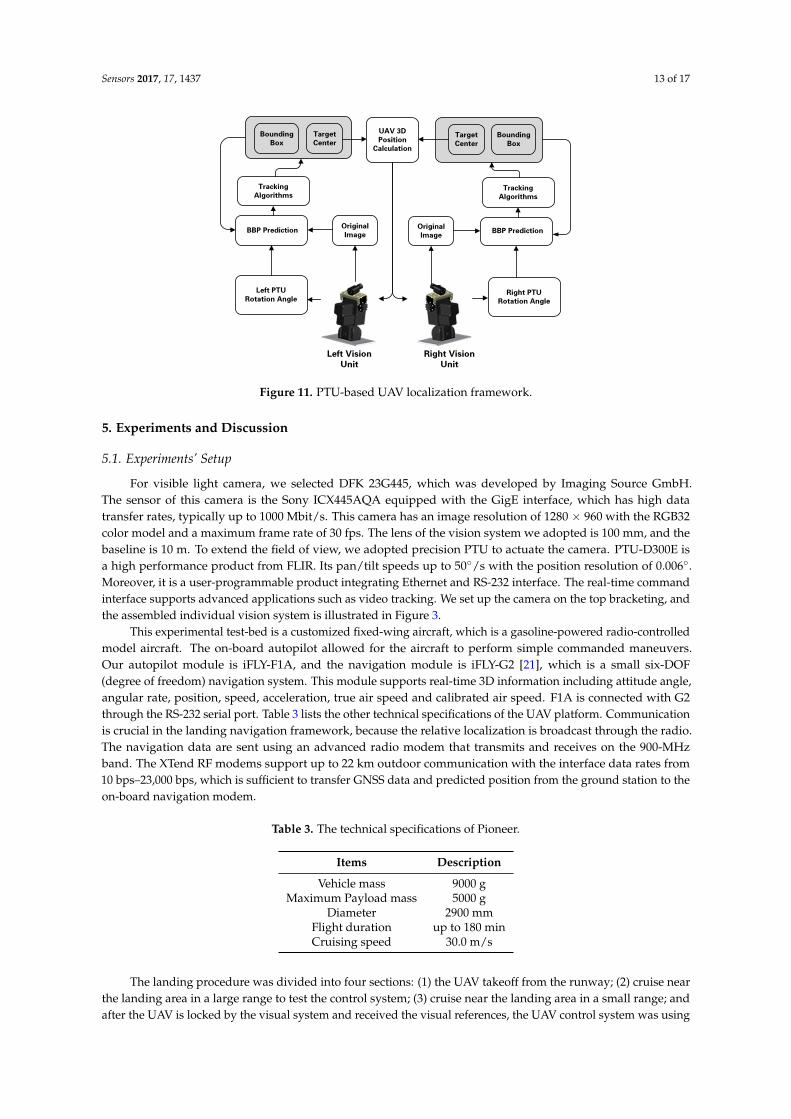
4.4. Localization Framework

In the ensemble configuration, we separate the vehicle guidance and control into an inner loop and an outerloop, because it is a much simpler and well-tested design approach. As the inner loop controller already exists inthe autopilot, we developed an efficient and robust outer navigation loop, which manages the visual informationwith the on-board sensors. Figure 11 presents the separated long baseline stereo localization frame.

Sensors 2017, 17, 1437 13 of 17

OriginalImage

TargetCenter

BoundingBox

Left PTURotation Angle

UAV 3DPosition

Calculation

OriginalImage

Right PTURotation Angle

Left VisionUnit

Right VisionUnit

TargetCenter

BoundingBox

BBP Prediction BBP Prediction

Tracking Algorithms

Tracking Algorithms

Figure 11. PTU-based UAV localization framework.

5. Experiments and Discussion

5.1. Experiments’ Setup

For visible light camera, we selected DFK 23G445, which was developed by Imaging Source GmbH.The sensor of this camera is the Sony ICX445AQA equipped with the GigE interface, which has high datatransfer rates, typically up to 1000 Mbit/s. This camera has an image resolution of 1280 × 960 with the RGB32color model and a maximum frame rate of 30 fps. The lens of the vision system we adopted is 100 mm, and thebaseline is 10 m. To extend the field of view, we adopted precision PTU to actuate the camera. PTU-D300E isa high performance product from FLIR. Its pan/tilt speeds up to 50◦/s with the position resolution of 0.006◦.Moreover, it is a user-programmable product integrating Ethernet and RS-232 interface. The real-time commandinterface supports advanced applications such as video tracking. We set up the camera on the top bracketing, andthe assembled individual vision system is illustrated in Figure 3.

This experimental test-bed is a customized fixed-wing aircraft, which is a gasoline-powered radio-controlledmodel aircraft. The on-board autopilot allowed for the aircraft to perform simple commanded maneuvers.Our autopilot module is iFLY-F1A, and the navigation module is iFLY-G2 [21], which is a small six-DOF(degree of freedom) navigation system. This module supports real-time 3D information including attitude angle,angular rate, position, speed, acceleration, true air speed and calibrated air speed. F1A is connected with G2through the RS-232 serial port. Table 3 lists the other technical specifications of the UAV platform. Communicationis crucial in the landing navigation framework, because the relative localization is broadcast through the radio.The navigation data are sent using an advanced radio modem that transmits and receives on the 900-MHzband. The XTend RF modems support up to 22 km outdoor communication with the interface data rates from10 bps–23,000 bps, which is sufficient to transfer GNSS data and predicted position from the ground station to theon-board navigation modem.

Table 3. The technical specifications of Pioneer.

Items Description

Vehicle mass 9000 gMaximum Payload mass 5000 g

Diameter 2900 mmFlight duration up to 180 minCruising speed 30.0 m/s

The landing procedure was divided into four sections: (1) the UAV takeoff from the runway; (2) cruise nearthe landing area in a large range to test the control system; (3) cruise near the landing area in a small range; andafter the UAV is locked by the visual system and received the visual references, the UAV control system was using

Sensors 2017, 17, 1437 14 of 17

vision-based localization data, and the GPS data was only recorded as the benchmark; (4) safely landing back onthe runway.

5.2. Results and Discussion

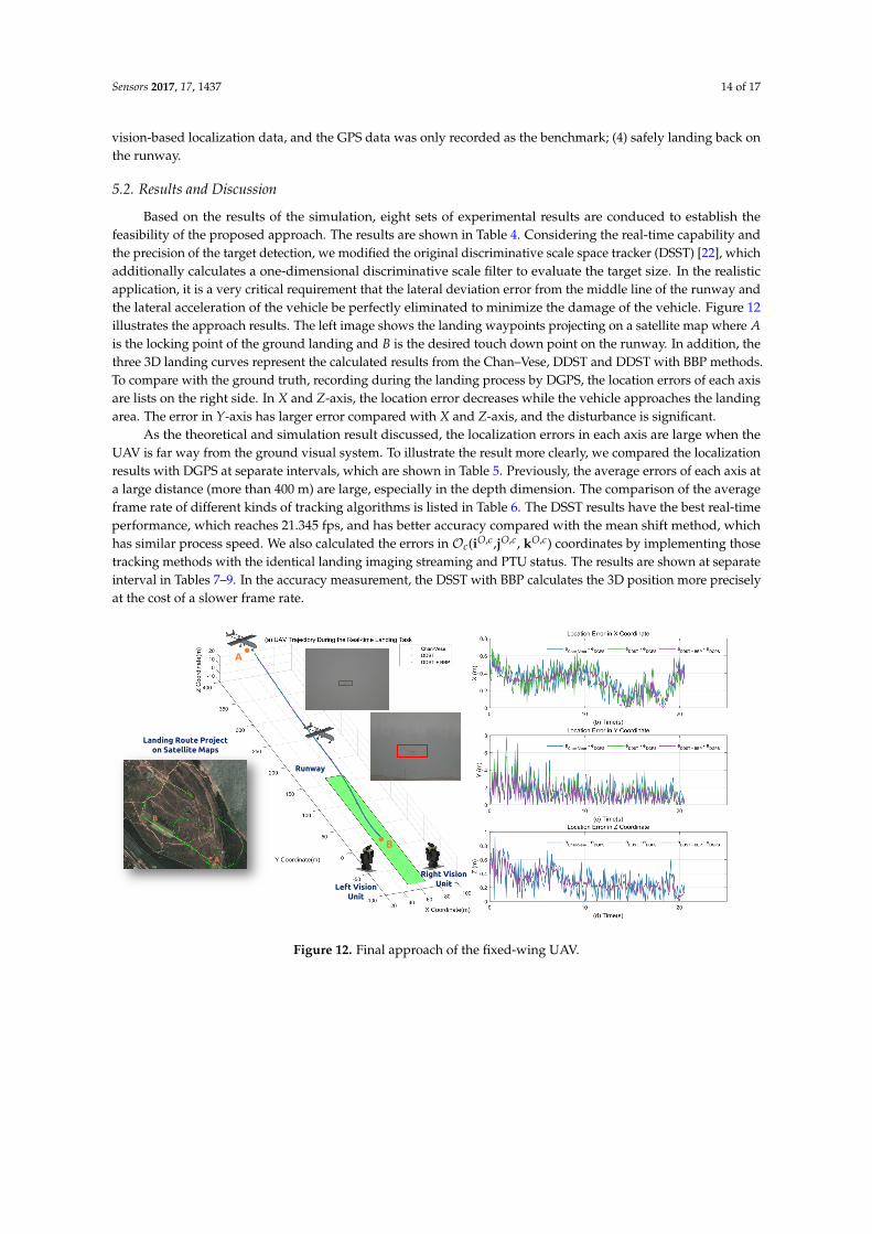
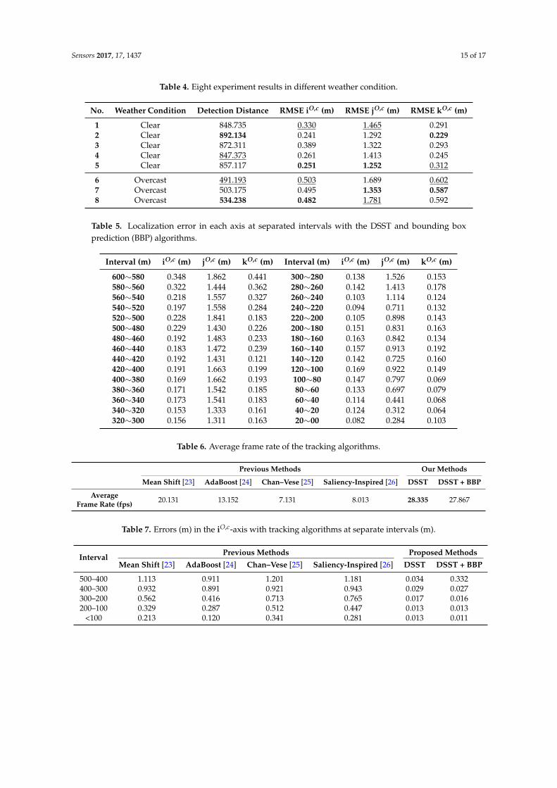
Based on the results of the simulation, eight sets of experimental results are conduced to establish thefeasibility of the proposed approach. The results are shown in Table 4. Considering the real-time capability andthe precision of the target detection, we modified the original discriminative scale space tracker (DSST) [22], whichadditionally calculates a one-dimensional discriminative scale filter to evaluate the target size. In the realisticapplication, it is a very critical requirement that the lateral deviation error from the middle line of the runway andthe lateral acceleration of the vehicle be perfectly eliminated to minimize the damage of the vehicle. Figure 12illustrates the approach results. The left image shows the landing waypoints projecting on a satellite map where Ais the locking point of the ground landing and B is the desired touch down point on the runway. In addition, thethree 3D landing curves represent the calculated results from the Chan–Vese, DDST and DDST with BBP methods.To compare with the ground truth, recording during the landing process by DGPS, the location errors of each axisare lists on the right side. In X and Z-axis, the location error decreases while the vehicle approaches the landingarea. The error in Y-axis has larger error compared with X and Z-axis, and the disturbance is significant.

As the theoretical and simulation result discussed, the localization errors in each axis are large when theUAV is far way from the ground visual system. To illustrate the result more clearly, we compared the localizationresults with DGPS at separate intervals, which are shown in Table 5. Previously, the average errors of each axis ata large distance (more than 400 m) are large, especially in the depth dimension. The comparison of the averageframe rate of different kinds of tracking algorithms is listed in Table 6. The DSST results have the best real-timeperformance, which reaches 21.345 fps, and has better accuracy compared with the mean shift method, whichhas similar process speed. We also calculated the errors in Oc(iO,c,jO,c, kO,c) coordinates by implementing thosetracking methods with the identical landing imaging streaming and PTU status. The results are shown at separateinterval in Tables 7–9. In the accuracy measurement, the DSST with BBP calculates the 3D position more preciselyat the cost of a slower frame rate.

B

A

Runway

Left VisionUnit

Right VisionUnit

B

A

Landing Route Projecton Satellite Maps

Figure 12. Final approach of the fixed-wing UAV.

Sensors 2017, 17, 1437 15 of 17

Table 4. Eight experiment results in different weather condition.

No. Weather Condition Detection Distance RMSE iO,c (m) RMSE jO,c (m) RMSE kO,c (m)

1 Clear 848.735 0.330 1.465 0.2912 Clear 892.134 0.241 1.292 0.2293 Clear 872.311 0.389 1.322 0.2934 Clear 847.373 0.261 1.413 0.2455 Clear 857.117 0.251 1.252 0.312

6 Overcast 491.193 0.503 1.689 0.6027 Overcast 503.175 0.495 1.353 0.5878 Overcast 534.238 0.482 1.781 0.592

Table 5. Localization error in each axis at separated intervals with the DSST and bounding boxprediction (BBP) algorithms.

Interval (m) iO,c (m) jO,c (m) kO,c (m) Interval (m) iO,c (m) jO,c (m) kO,c (m)

600∼580 0.348 1.862 0.441 300∼280 0.138 1.526 0.153580∼560 0.322 1.444 0.362 280∼260 0.142 1.413 0.178560∼540 0.218 1.557 0.327 260∼240 0.103 1.114 0.124540∼520 0.197 1.558 0.284 240∼220 0.094 0.711 0.132520∼500 0.228 1.841 0.183 220∼200 0.105 0.898 0.143500∼480 0.229 1.430 0.226 200∼180 0.151 0.831 0.163480∼460 0.192 1.483 0.233 180∼160 0.163 0.842 0.134460∼440 0.183 1.472 0.239 160∼140 0.157 0.913 0.192440∼420 0.192 1.431 0.121 140∼120 0.142 0.725 0.160420∼400 0.191 1.663 0.199 120∼100 0.169 0.922 0.149400∼380 0.169 1.662 0.193 100∼80 0.147 0.797 0.069380∼360 0.171 1.542 0.185 80∼60 0.133 0.697 0.079360∼340 0.173 1.541 0.183 60∼40 0.114 0.441 0.068340∼320 0.153 1.333 0.161 40∼20 0.124 0.312 0.064320∼300 0.156 1.311 0.163 20∼00 0.082 0.284 0.103

Table 6. Average frame rate of the tracking algorithms.

Previous Methods Our Methods

Mean Shift [23] AdaBoost [24] Chan–Vese [25] Saliency-Inspired [26] DSST DSST + BBP

AverageFrame Rate (fps) 20.131 13.152 7.131 8.013 28.335 27.867

Table 7. Errors (m) in the iO,c-axis with tracking algorithms at separate intervals (m).

Interval Previous Methods Proposed MethodsMean Shift [23] AdaBoost [24] Chan–Vese [25] Saliency-Inspired [26] DSST DSST + BBP

500–400 1.113 0.911 1.201 1.181 0.034 0.332400–300 0.932 0.891 0.921 0.943 0.029 0.027300–200 0.562 0.416 0.713 0.765 0.017 0.016200–100 0.329 0.287 0.512 0.447 0.013 0.013

<100 0.213 0.120 0.341 0.281 0.013 0.011

Sensors 2017, 17, 1437 16 of 17

Table 8. Errors (m) in the jO,c-axis with tracking algorithms at separate intervals (m).

Interval Previous Methods Proposed MethodsMean Shift [23] AdaBoost [24] Chan–Vese [25] Saliency-Inspired [26] DSST DSST + BBP

500–400 11.923 6.238 3.661 3.231 2.218 1.761400–300 7.317 5.721 2.887 2.902 1.876 1.632300–200 5.365 2.576 1.799 1.767 1.703 1.371200–100 3.897 1.739 1.310 1.134 0.981 1.131

<100 1.762 0.780 0.737 0.692 0.763 0.541

Table 9. Errors (m) in the kO,c-axis with tracking algorithms at separate intervals (m).

Interval Previous Methods Proposed MethodsMean Shift [23] AdaBoost [24] Chan–Vese [25] Saliency-Inspired [26] DSST DSST + BBP

500–400 1.231 1.087 1.387 1.299 0.487 0.484400–300 0.976 0.901 0.762 0.876 0.370 0.325300–200 0.812 0.557 0.337 0.612 0.459 0.313200–100 0.438 0.312 0.489 0.532 0.141 0.179

<100 0.301 0.211 0.401 0.321 0.102 0.103

6. Concluding Remarks

This paper presents a complete localization framework of the ground-based stereo guidance system.This system could be used to pilot the UAV for landing autonomously and safely in the GNSS-denied scenario.Compared with the onboard solutions and other state-of-the-art ground-based approaches, this ground-basedsystem profited enormously from the computation capacity and flexible configuration with the baseline andsensors. The separate deployed configurations did not improve the detection distance, which was discussed inour previous works [15]; however, they enhance the maximum range for depth estimation. Although the systemhas some pitfalls, such as the low accuracy at a long distance in the depth axis and not supporting the attitudemeasurement, this low-cost system could be arranged quickly for any proposed environment. Additional futurework will focus on estimate errors over time and investigate methods to improve inevitable error propagationthrough the inclusion of additional sensors, such as GNSS and on-board sensors.

Acknowledgments: The work is supported by Major Application Basic Research Project of NUDT with GrantedNo. ZDYYJCYJ20140601. The authors would like to thank Dianle Zhou and Zhiwei Zhong for their contributionon the experimental prototype development. Tengxiang Li, Dou Hu, Shao Hua and Yexun Xi made a greatcontribution on the practical experiment configuration.

Author Contributions: W.K. proposed and designed the ground-based navigation system architecture. W.K.and T.H. implemented the vision algorithms to test the capability of the system. D.Z., L.S., and J.Z. participatedin the development of the guidance system and conceive the experiments. All authors read and approved thefinal manuscript.

Conflicts of Interest: The authors declare no conflict of interest.The authors declare no conflict of interest.The founding sponsors had no role in the design of the study; in the collection, analyses, or interpretation of data;in the writing of the manuscript, and in the decision to publish the results.

References

1. Floreano, D.; Wood, R.J. Science, technology and the future of small autonomous drones. Nature 2015,521, 460–466.

2. Kushleyev, A.; Mellinger, D.; Powers, C.; Kumar, V. Towards a swarm of agile micro quadrotors. Auton. Robot.2013, 35, 287–300.

3. Manning, S.D.; Rash, C.E.; LeDuc, P.A.; Noback, R.K.; McKeon, J. The Role of Human Causal Factors in USArmy Unmanned Aerial Vehicle Accidents; Army Aeromedical Research Lab: Fort Rucker, AL, USA, 2004.

4. McLean, D. Automatic Flight Control Systems; Prentice Hall: Englewood Cliffs, NJ, USA, 1990; p. 6065. Stevens, B.L.; Lewis, F.L. Aircraft Control and Simulation; John Wiley & Sons: Hoboken, NJ, USA, 2003.6. Farrell, J.; Barth, M.; Galijan, R.; Sinko, J. GPS/INS Based Lateral and Longitudinal Control Demonstration:

Final Report; California Partners for Advanced Transit and Highways (PATH): Richmond, CA, USA, 1998.

Sensors 2017, 17, 1437 17 of 17

7. RUAG. Available online: https://www.ruag.com/de/node/307 (accessed on 8 June 2017).8. Northrop Grumman. MQ-8B Fire Scout Vertical Takeoff and Landing Tactical Unmanned Aerial Vehicle System;

Northrop Grumman: Falls Church, VA, USA.9. Wang, W.; Song, G.; Nonami, K.; Hirata, M.; Miyazawa, O. Autonomous Control for Micro-Flying Robot

and Small Wireless Helicopter X.R.B. In Proceedings of the 2006 IEEE/RSJ International Conference onIntelligent Robots and Systems, Beijing, China, 9–15 October 2006; pp. 2906–2911.

10. Pebrianti, D.; Kendoul, F.; Azrad, S.; Wang, W.; Nonami, K. Autonomous hovering and landing ofa quad-rotor micro aerial vehicle by means of on ground stereo vision system. J. Syst. Des. Dyn. 2010,4, 269–284.

11. Martinez, C.; Campoy, P.; Mondragon, I.; Olivares-Mendez, M.A. Trinocular ground system to control UAVs.In Proceedings of the 2009 IEEE/RSJ International Conference on Intelligent Robots and Systems, St. Louis,MO, USA, 10–15 October 2009; pp. 3361–3367.

12. Guan, B.; Sun, X.; Shang, Y.; Zhang, X.; Hofer, M. Multi-camera networks for motion parameter estimationof an aircraft. Int. J. Adv. Robot. Syst. 2017, 14, doi:10.1177/1729881417692312.

13. Kim, E.; Choi, D. A UWB positioning network enabling unmanned aircraft systems auto land.Aerosp. Sci. Technol. 2016, 58, 418–426.

14. Kong, W.; Zhang, D.; Wang, X.; Xian, Z.; Zhang, J. Autonomous landing of an UAV with a ground-basedactuated infrared stereo vision system. In Proceedings of the 2013 IEEE/RSJ International Conference onIntelligent Robots and Systems, Tokyo, Japan, 3–7 November 2013; pp. 2963–2970.

15. Kong, W.; Zhou, D.; Zhang, Y.; Zhang, D.; Wang, X.; Zhao, B.; Yan, C.; Shen, L.; Zhang, J. A ground-basedoptical system for autonomous landing of a fixed wing UAV. In Proceedings of the 2014 IEEE/RSJInternational Conference on Intelligent Robots and Systems, Chicago, IL, USA, 14–18 September 2014;pp. 4797–4804.

16. Tang, D.; Hu, T.; Shen, L.; Zhang, D.; Kong, W.; Low, K.H. Ground Stereo Vision-based Navigation forAutonomous Take-off and Landing of UAVs: A Chan-Vese Model Approach. Int. J. Adv. Robot. Syst. 2016,13, doi:10.5772/62027.

17. Ma, Z.; Hu, T.; Shen, L. Stereo vision guiding for the autonomous landing of fixed-wing UAVs:A saliency-inspired approach. Int. J. Adv. Robot. Syst. 2016, 13, 43.

18. Kong, W.; Zhou, D.; Zhang, D.; Zhang, J. Vision-based autonomous landing system for unmannedaerial vehicle: A survey. In Proceedings of the 2014 International Conference on Multisensor Fusionand Information Integration for Intelligent Systems (MFI), Beijing, China, 28–29 September 2014; pp. 1–8.

19. Gautam, A.; Sujit, P.; Saripalli, S. A survey of autonomous landing techniques for UAVs. In Proceedings of the2014 International Conference on Unmanned Aircraft Systems (ICUAS), Orlando, FL, USA, 27–30 May 2014;pp. 1210–1218.

20. Hu, T.; Zhao, B.; Tang, D.; Zhang, D.; Kong, W.; Shen, L. ROS-based ground stereo vision detection:Implementation and experiments. Robot. Biomim. 2016, 3, 14.

21. Beijing Universal Pioneering Technology Co., Ltd. iFLYUAS; Beijing Universal Pioneering Technology Co., Ltd.:Beijing, China, 2016.

22. Danelljan, M.; Häger, G.; Khan, F.; Felsberg, M. Accurate scale estimation for robust visual tracking. In BritishMachine Vision Conference, Nottingham, 1–5 September 2014; BMVA Press: Durham, UK, 2014.

23. Oza, N.C. Online bagging and boosting. In Proceedings of the 2005 IEEE International Conference onSystems, Man and Cybernetics, Waikoloa, HI, USA, 10–12 October 2005; Volume 3, pp. 2340–2345.

24. Bradski, G.R. Real time face and object tracking as a component of a perceptual user interface.In Proceedings of the IEEE Workshop on Applications of Computer Vision (WACV’98), Princeton, NJ,USA, 19–21 October 1998; pp. 214–219.

25. Chan, T.F.; Sandberg, B.Y.; Vese, L.A. Active contours without edges for vector-valued images. J. Vis.Commun. Image Represent. 2000, 11, 130–141.

26. Itti, L.; Koch, C.; Niebur, E. A model of saliency-based visual attention for rapid scene analysis. IEEE Trans.Pattern Anal. Mach. Intell. 1998, 20, 1254–1259.

c© 2017 by the authors. Licensee MDPI, Basel, Switzerland. This article is an open accessarticle distributed under the terms and conditions of the Creative Commons Attribution(CC BY) license (http://creativecommons.org/licenses/by/4.0/).