Estimation of Flaring
59
Guide Estimation of Flaring and Venting Volumes from Upstream Oil and Gas Facilities May 2002 2002-0009
Transcript of Estimation of Flaring
8/3/2019 Estimation of Flaring
http://slidepdf.com/reader/full/estimation-of-flaring 1/59
Guide
Estimation of Flaring and
Venting Volumes from UpstreamOil and Gas Facilities
May 2002
2002-0009
8/3/2019 Estimation of Flaring
http://slidepdf.com/reader/full/estimation-of-flaring 2/59
Disclaimer
This publication was prepared for the Canadian Association of PetroleumProducers (CAPP) by Clearstone Engineering Ltd. While it is believed that theinformation contained herein is reliable under the conditions and subject to thelimitations set out, CAPP and Clearstone Engineering do not guarantee itsaccuracy. The use of this report or any information contained will be at the user’ssole risk, regardless of any fault or negligence of Clearstone Engineering Ltd.,CAPP or its co-funders.
Review by July, 2005
2100, 350 – 7th Ave. S.W.Calgary, AlbertaCanada T2P 3N9Tel (403) 267-1100Fax (403) 261-4622
230, 1801 Hollis StreetHalifax, Nova ScotiaCanada B3J 3N4Tel (902) 420-9084Fax (902) 491-2980
905, 235 Water StreetSt. John’s, NewfoundlandCanada A1C 1B6Tel (709) 724-4200Fax (709) 724-4225
Email: [email protected] Website: www.capp.ca
The Canadian Association of Petroleum Producers (CAPP) represents 140
companies that explore for, develop and produce natural gas, natural gas liquids,
crude oil, oil sands, and elemental sulphur throughout Canada. CAPP member
companies produce over 97 per cent of Canada’s natural gas and crude oil. CAPP
also has 125 associate members that provide a wide range of services that support
the upstream crude oil and natural gas industry. Together, these members andassociate members are an important part of a $52-billion-a-year national industry
that affects the livelihoods of more than half a million Canadians.

8/3/2019 Estimation of Flaring
http://slidepdf.com/reader/full/estimation-of-flaring 3/59Page 3
May 2002 Estimation of Flaring and Venting Volumes
from Upstream Oil and Gas Facilities
Overview
This handbook is presented to assist oil and gas production companies in
quantifying volumes of natural gas vented and flared at typical upstream oil and
gas facilities.
The following have been identified as continuous sources of vented and flared gas:
Continuous Sources
Casing Gas Vents,•Associated/Solution Gas,•Venting from Glycol Dehydrators,•Production Storage Tanks, and•Pneumatic Devices.•
The following have been identified as intermittent venting/flaring sources.
Intermittent Sources
Well Blowdowns,•Accidental Releases,•Pressure Relief/Pressure Safety Valves, and•Facility Blowdowns.•
The focus of this document is to provide methodologies and example calculations
for estimating volumes of gas released from each of the sources listed above. For
each source a variety of estimation methods are presented ranging from simple
emission factors to complex process simulation. This is not, however, anexhaustive compendium of all possible estimation methods.
In most cases, the simple methods should be adequate. Occasionally, the more
complex methods may be appropriate. The intent is simply to present some of the
valid alternatives rather than to prescribe measurement methods. Companies
should choose the approaches best suited to their particular situations, and the
relative importance of the given sources.
8/3/2019 Estimation of Flaring
http://slidepdf.com/reader/full/estimation-of-flaring 4/59Page 4
May 2002 Estimation of Flaring and Venting Volumes
from Upstream Oil and Gas Facilities
Contents
1 Introduction 1-1
2 Source Characterization 2-1
2.1 Wells 2-1
2.2 Oil Production Facilities 2-1
2.3 Gas Production Facilities 2-2
2.4 Gas Processing Plants 2-3
2.5 Relative Magnitude of Flaring/Venting Volumes 2-3
3 Assessment Procedures 3-1
3.1 Continuous Sources 3-1
3.1.1 Casing Gas Vents 3-1
3.1.2 Associated/Solution Gas 3-33.1.3 Venting from Glycol Dehydrators 3-9
3.1.4 Production Storage Tanks 3-10
3.1.5 Pneumatic Devices 3-17
3.2 Intermittent Sources 3-19
3.2.1 Well Blowdowns 3-19
3.2.2 Accidental Releases 3-23
3.2.3 Pressure Relief/Pressure Safety Valves 3-26
3.2.4 Facility Blowdowns 3-27
Figures
Figure 3-1 Process Diagram Showing the Information Requirements for Estimating
Flashing Losses From Oil Storage Tanks Using E&P Tank 3-14
Figure 3-2 Schematic Diagram Showing Information Requirements for Estimating
Flashing Losses From Oil Storage Tanks Using a Process Simulator 3-14
Tables
Table 1-1 Summary of EUB ID 94-01 Measurement Criteria 1-1
Table 2-1 Summary of Potential Flare and Vent Gas Sources 2-3
Table 2-2 Summary of Flare and Vent Volumes for 2000 2-4
Table 3-1 Summary of Possible Casing Gas Measurement Methods 3-2
Table 3-2 Summary of Range of Data Used to Develop Each of the Correlations 3-4
Table 3-3 A List of Several Commercially-Available Process Simulation Packages 3-6
Table 3-4 Average Vent Rates for Pneumatic Devices Based on Data Collected in
8/3/2019 Estimation of Flaring
http://slidepdf.com/reader/full/estimation-of-flaring 5/59Page 5
May 2002 Estimation of Flaring and Venting Volumes
from Upstream Oil and Gas Facilities
Alberta 3-18
Table 3-5 Typical Number of Pneumatic Devices at Various Types of Upstream Oil
and Gas Facilities 3-18
Table 3-6 Summary of Typical Vent Rates From Pneumatic Instruments at Various
Facility Types. 3-19
Table 3-7 Summary of Cross-Sectional Areas for Typical Pipe Sizes 3-22Table 3-8 Volume Occupied by a One-Metre Length of Various Standard Pipe Sizes 3-28
Table 3-9 Correlation Coefficients for Estimating Compressibility Factors for Typical
Gas Plant Inlet Gas. 3-31

8/3/2019 Estimation of Flaring
http://slidepdf.com/reader/full/estimation-of-flaring 6/59
May 2002 Estimation of Flaring and Venting Volumes Page 6
from Upstream Oil and Gas Facilities
Introduction1
In June 1999 the Alberta Energy and Utilities Board released Guide 60: Upstream
Petroleum Industry Flaring Requirements. The guide (G-60) outlines the
requirements and expectations of oil and gas operators with regard to flaring. The
following is a brief summary of the G-60 requirements:
A firm provincial solution gas volume reduction schedule. A 15 percent•reduction from 1996 levels by the end of 2000 and a 25 percent reduction by
the end of 2001.
New performance requirements for all flares.•Evaluation of all solution gas flares using a flaring management decision tree•by December 31, 2002 and all other flares by December 31, 2004.
As part of these general requirements, all operators are expected to ensure that
flared and vented gas volumes from all operations are accurately reported on the
appropriate production accounting reports (i.e., S-Reports).
As per EUB ID 94-01, the EUB has established maximum uncertainty limits for
different streams. The requirements for gas measurement are outlined below:
Table 1-1 Summary of EUB ID 94-01 Measurement Criteria
EUB ID 94-01 Summary
BatteryType Gas Rate Gas Type Uncertainty
Allowed (%)
oil >0.5 e3m3 /day battery sales 3
oil >0.5 e3m3 /day battery flare 5
oil <0.5 e3m3 /day battery stream 20
oil >16.9 e3m3 /day well 3
oil <0.5 e3m3 /day
&
>16.9 e3m3 /day
well 5
oil <0.5 e3m3 /day well 20
gas any battery 3
gas >16.9 e3m3 /day well 3
gas < 16.9 e3m3 /day well 5
Notwithstanding the above uncertainty limits, the EUB requires operators to report
gas flared or vented to the nearest 0.1 e3 m3 per month (at standard conditions of
101.325 kPa and 15ºC). The requirement to report all vented or flared gas
includes volumes from routine operations, emergency conditions, and the
8/3/2019 Estimation of Flaring
http://slidepdf.com/reader/full/estimation-of-flaring 7/59
May 2002 Estimation of Flaring and Venting Volumes Page 7
from Upstream Oil and Gas Facilities
depressurization of pipeline, compression and processing systems. Note that the
EUB intends to release an update to ID 94-01 in 2002 to address measurement
accuracy issues.
As per Guide 60 Section 10.1.1, the following streams should generally be
metered:Acid gas flared1)
Make-up gas for acid gas flaring2)
Routine flares in conventional oil and gas facilities where average annual3)
volumes exceed 0.5 e3m3/day
Heavy oil or bitumen solution gas where the average annual volume exceeds4)
2.0 e3m3/day.
Where operators can show these flows can be accurately estimated the EUB may
accept estimated measurements. It is preferred that other flared and vented gas be
metered with appropriate measurement equipment. However, where it is not
practicable to meter the vented or flared gas, accurate estimates of the gas volumesare acceptable to the EUB. If volume estimation methods are used, operators
must be able to demonstrate that a reliable and accurate flare or vent gas
estimating-and-reporting system is in place and that it is consistently used.
The intention of this document is to provide guidance to CAPP members that
require assistance with estimation of flared and vented gas volumes. This guide
does not provide an exhaustive compendium of flared and vented gas volume
estimation methods. Therefore, operators may choose alternate estimation
methods. The methods presented for each source are described in the order of
increasing sophistication and accuracy. Operators should select the most
appropriate methodology considering the magnitude of the volume being
estimated. In general, the simplest method will suffice.
Section 2 provides an overview of the sources of vented and flared gas volumes at
upstream oil and gas facilities. Each of the sources is described in Section 3 along
with suggested estimation methods and sample calculations.

8/3/2019 Estimation of Flaring
http://slidepdf.com/reader/full/estimation-of-flaring 8/59
May 2002 Estimation of Flaring and Venting Volumes Page 8
from Upstream Oil and Gas Facilities
Source Characterization2
The upstream oil and gas industry comprises all infrastructure used to find,
produce, process/treat and transport natural gas, liquified petroleum gas,
condensate, crude oil, heavy oil and crude bitumen to market. The industry may
be divided into several sectors depending on the types of activities that areperformed:
wells,•oil production facilities,•gas production facilities, and•gas processing plants.•
Each of these sectors may have several potential sources of vented or flared gas
that must be reported to EUB as part of the production accounting process. The
following sections provide a brief description of each of the sectors. The potential
sources of flared/vented gas for each sector are presented in Table 1.
Wells2.1
A well site is a surface facility that is used to produce oil and gas from a
hydrocarbon reservoir. It consists of the wellhead and may or may not have
metering facilities and some production equipment (e.g., pumpjack, compressor,
line heater, dehydrator, storage tank, etc).
Oil Production Facilities2.2
A battery is a production unit where the effluent from a well(s) is separated into itsconstituent phases (oil, gas and water) for metering and appropriate disposition.
The oil is pumped into a nearby crude oil pipeline, or is shipped by truck to a
location where this may be done. A treater is used to remove any emulsified water
from the oil before it is put in the crude oil pipeline. The gas is either flared,
reinjected, or compressed into a nearby gas gathering system, depending on the
type of oil recovery scheme and the economics of the situation. The last two
options would require that compression and, possibly, dehydration facilities be
installed. The water is reinjected as part of an enhanced recovery scheme, or is
shipped to a nearby disposal well.
A single-well production unit is the simplest type of oil battery. Typically, each isinspected once per day; otherwise, it is unattended. At a minimum, it is equipped
with separation, metering, storage, loading and flaring facilities. Depending on the
amount and nature of the production, it may also comprise selected treatment,
pumping and compression facilities.
A satellite battery is an intermediate production facility. It is located between a
group of wells and a central battery, and, usually, it is inspected once per day.

8/3/2019 Estimation of Flaring
http://slidepdf.com/reader/full/estimation-of-flaring 9/59
May 2002 Estimation of Flaring and Venting Volumes Page 9
from Upstream Oil and Gas Facilities
There are two separators and associated sets of metering equipment at each
satellite battery. One train is used to compile proration data on the commingled
effluent from all but one of the group of wells. The other is used to test the
remaining well. A regular test is performed on each of the wells.
After separation and measurement, the production is often recombined into asingle flow line for shipment to the central battery. Sometimes, however, each
phase is transported in a separate pipeline. In this case a dehydrator may be
required for the gas pipeline. Typically, there are no storage nor treatment facilities
at satellite batteries, and no gas is flared. Consequently, the only source of vented
gas is the use of fuel gas to operate instrument controllers.
A central battery is the same as a single-well battery except that it receives
production from more than one well and is usually much larger. Often, it is
manned continuously during the day.
Gas Production Facilities2.3
The surface pressure, flowing temperature and composition of natural gas at a well
have a strong influence on the equipment required to handle and transmit the well
effluent to a gas processing plant. These factors are also critical to the formation of
hydrates in the production tubing, vessels, piping and pipeline. The types of
gathering systems may be categorized as low pressure, heated and dehydrated
systems.
There is a substantial network of low pressure pipelines used to gather production
from shallow gas wells. These systems are often operated at very low pressures
(e.g., less than 525 kPa).
Heated gathering systems guard against the formation of hydrates by maintaining
the gas temperature above some critical value. This critical value is dependent on
the composition and pressure of the gas. Consequently, this value varies from one
system to the next.
Dehydrated gathering systems prevent the formation of hydrates by removing
water vapour from the process gas. There are several different dehydration
technologies that are used: absorption using diethylene or triethylene glycol;
adsorption using solid desiccants such as activated alumina, gels, or molecular
sieve; and the chem-sorption process using calcium chloride. The glycol-basedabsorption process is the most widely used.
A gas battery is a production unit that is used when gas processing is not required.
Only compression and simple treating (e.g., dehydration and/or non-regenerative
sweetening with less than 0.1 tonnes/day total Sulphur) may be needed to upgrade
gas to market specifications. Typically, this type of gas comes from low-pressure,
shallow gas wells. It is characterized by low concentrations of non-methane

8/3/2019 Estimation of Flaring
http://slidepdf.com/reader/full/estimation-of-flaring 10/59
May 2002 Estimation of Flaring and Venting Volumes Page 10
from Upstream Oil and Gas Facilities
hydrocarbons and is called "dry gas."
The basic functions of a gas battery are to separate the effluent from one or more
gas wells into gas and water, measure the flow rate of each of these phases from
each well, and provide any gas treating and compression that may be required.
The water is disposed of and the gas is sent to market.
Gas Processing Plants2.4
A gas processing plant is a facility for extracting condensable hydrocarbons from
natural gas, and for upgrading the quality of the gas to market specifications (i.e.,
removing contaminants such as H2O, H2S and CO2). Some compression may also
be required. Each facility may comprise a variety of treatment and extraction
processes, and for each of these there is often a range of technologies that may be
used.
There are several types of gas processing facilities: sweet plants, sour plants thatflare their waste gas, sour plants that extract elemental sulphur from their waste
gas, sour plants that inject the acid gas into a subsurface formation and straddle
plants. The first four types are fed by gathering systems and prepare natural gas
for transmission to market. The last type is located on major gas transmission lines
and is used to extract residual ethane and heavier hydrocarbons from the natural
gas.
Relative Magnitude of Flaring/Venting Volumes2.5
To determine where estimation efforts should be focused it is important to
understand where each emission source may be found and the relative magnitudeof each source. Table 2-1 provides a summary of potential sources of
flared/vented gas for each sector of the upstream oil and gas industry.
Table 2-1 Summary of Potential Flare and Vent Gas Sources by Sector
Flared/Vented Gas Source Wells Oil
Production
Gas
Production
Gas
Processing
Continuous Sources
Casing Gas Venting P
Solution Gas P P P P
Glycol Dehydrator Off-Gas P P P
SCVF’s P
Gas Migration P
Production Storage Tanks P P P P
8/3/2019 Estimation of Flaring
http://slidepdf.com/reader/full/estimation-of-flaring 11/59
May 2002 Estimation of Flaring and Venting Volumes Page 11
from Upstream Oil and Gas Facilities
Pneumatic Devices (i.e., controllers,chemical injection pumps)
P P P P
Intermittent Sources
Well Blowouts P
Well BlowdownsP
Pipeline Ruptures P P P P
Pressure Relief/Pressure SafetyValves
P P P
Blowdowns of Process Vessels andPiping / Upsets
P P P
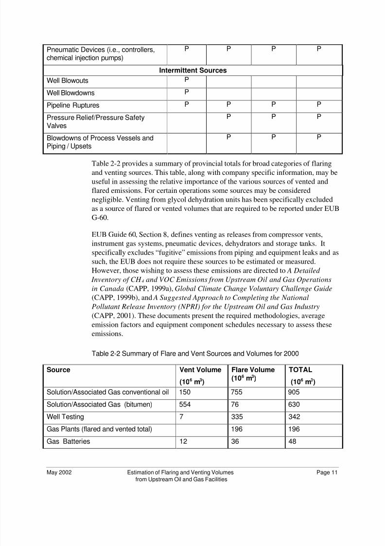
Table 2-2 provides a summary of provincial totals for broad categories of flaring
and venting sources. This table, along with company specific information, may be
useful in assessing the relative importance of the various sources of vented and
flared emissions. For certain operations some sources may be considerednegligible. Venting from glycol dehydration units has been specifically excluded
as a source of flared or vented volumes that are required to be reported under EUB
G-60.
EUB Guide 60, Section 8, defines venting as releases from compressor vents,
instrument gas systems, pneumatic devices, dehydrators and storage tanks. It
specifically excludes “fugitive” emissions from piping and equipment leaks and as
such, the EUB does not require these sources to be estimated or measured.
However, those wishing to assess these emissions are directed to A Detailed
Inventory of CH 4 and VOC Emissions from Upstream Oil and Gas Operations
in Canada (CAPP, 1999a), Global Climate Change Voluntary Challenge Guide (CAPP, 1999b), and A Suggested Approach to Completing the National
Pollutant Release Inventory (NPRI) for the Upstream Oil and Gas Industry
(CAPP, 2001). These documents present the required methodologies, average
emission factors and equipment component schedules necessary to assess these
emissions.
Table 2-2 Summary of Flare and Vent Sources and Volumes for 2000
Source Vent Volume
(106
m3
)
Flare Volume
(106 m3)
TOTAL
(106
m3
)Solution/Associated Gas conventional oil 150 755 905
Solution/Associated Gas (bitumen) 554 76 630
Well Testing 7 335 342
Gas Plants (flared and vented total) 196 196
Gas Batteries 12 36 48
8/3/2019 Estimation of Flaring
http://slidepdf.com/reader/full/estimation-of-flaring 12/59
May 2002 Estimation of Flaring and Venting Volumes Page 12
from Upstream Oil and Gas Facilities
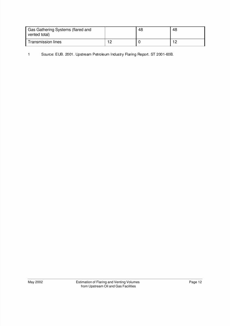
Gas Gathering Systems (flared andvented total)
48 48
Transmission lines 12 0 12
1 Source: EUB. 2001. Upstream Petroleum Industry Flaring Report. ST 2001-60B.
8/3/2019 Estimation of Flaring
http://slidepdf.com/reader/full/estimation-of-flaring 13/59Page 13
May 2002 Estimation of Flaring and Venting Volumes
from Upstream Oil and Gas Facilities
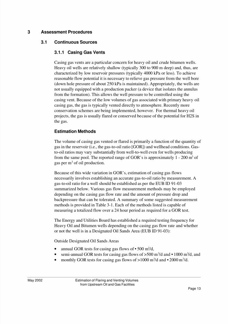
Assessment Procedures3
Continuous Sources3.1
Casing Gas Vents3.1.1
Casing gas vents are a particular concern for heavy oil and crude bitumen wells.
Heavy oil wells are relatively shallow (typically 300 to 900 m deep) and, thus, are
characterized by low reservoir pressures (typically 4000 kPa or less). To achieve
reasonable flow potential it is necessary to relieve gas pressure from the well bore
(down hole pressure of about 250 kPa is maintained). Appropriately, the wells are
not usually equipped with a production packer (a device that isolates the annulus
from the formation). This allows the well pressure to be controlled using the
casing vent. Because of the low volumes of gas associated with primary heavy oil
casing gas, the gas is typically vented directly to atmosphere. Recently more
conservation schemes are being implemented, however. For thermal heavy oil
projects, the gas is usually flared or conserved because of the potential for H2S in
the gas.
Estimation Methods
The volume of casing gas vented or flared is primarily a function of the quantity of
gas in the reservoir (i.e., the gas-to-oil ratio [GOR]) and wellhead conditions. Gas-
to-oil ratios may vary substantially from well-to-well even for wells producing
from the same pool. The reported range of GOR’s is approximately 1 - 200 m3 of
gas per m3 of oil production.
Because of this wide variation in GOR’s, estimation of casing gas flows
necessarily involves establishing an accurate gas-to-oil ratio by measurement. A
gas-to-oil ratio for a well should be established as per the EUB ID 91-03
summarized below. Various gas flow measurement methods may be employed
depending on the casing gas flow rate and the amount of pressure drop and
backpressure that can be tolerated. A summary of some suggested measurement
methods is provided in Table 3-1. Each of the methods listed is capable of
measuring a totalized flow over a 24 hour period as required for a GOR test.
The Energy and Utilities Board has established a required testing frequency for
Heavy Oil and Bitumen wells depending on the casing gas flow rate and whetheror not the well is in a Designated Oil Sands Area (EUB ID 91-03):
Outside Designated Oil Sands Areas
annual GOR tests for casing gas flows of • 500 m3 /d,•semi-annual GOR tests for casing gas flows of >500 m3 /d and • 1000 m3 /d, and•monthly GOR tests for casing gas flows of >1000 m3 /d and • 2000 m3 /d.•
8/3/2019 Estimation of Flaring
http://slidepdf.com/reader/full/estimation-of-flaring 14/59Page 14
May 2002 Estimation of Flaring and Venting Volumes
from Upstream Oil and Gas Facilities
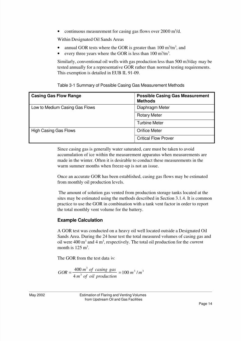
continuous measurement for casing gas flows over 2000 m3 /d.•
Within Designated Oil Sands Areas
annual GOR tests where the GOR is greater than 100 m3 /m3, and•every three years where the GOR is less than 100 m3 /m3.•
Similarly, conventional oil wells with gas production less than 500 m3/day may betested annually for a representative GOR rather than normal testing requirements.
This exemption is detailed in EUB IL 91-09.
Table 3-1 Summary of Possible Casing Gas Measurement Methods
Casing Gas Flow Range Possible Casing Gas Measurement
Methods
Low to Medium Casing Gas Flows Diaphragm Meter
Rotary Meter
Turbine Meter
High Casing Gas Flows Orifice Meter
Critical Flow Prover
Since casing gas is generally water saturated, care must be taken to avoid
accumulation of ice within the measurement apparatus when measurements are
made in the winter. Often it is desirable to conduct these measurements in the
warm summer months when freeze-up is not an issue.
Once an accurate GOR has been established, casing gas flows may be estimated
from monthly oil production levels.
The amount of solution gas vented from production storage tanks located at the
sites may be estimated using the methods described in Section 3.1.4. It is common
practice to use the GOR in combination with a tank vent factor in order to report
the total monthly vent volume for the battery.
Example Calculation
A GOR test was conducted on a heavy oil well located outside a Designated Oil
Sands Area. During the 24 hour test the total measured volumes of casing gas and
oil were 400 m3 and 4 m3, respectively. The total oil production for the current
month is 125 m3.
The GOR from the test data is:
33
3
3
/ 1004
400mm
productionoilof m
gasingcasof mGOR ==

8/3/2019 Estimation of Flaring
http://slidepdf.com/reader/full/estimation-of-flaring 15/59Page 15
May 2002 Estimation of Flaring and Venting Volumes
from Upstream Oil and Gas Facilities
The estimated casing gas vent rate for the current month is then:
V=GOR production
V=100M 3 /m3 125m3
V= 12.5 X 10³ m3
Note: Since the measured daily casing gas flow rate is • 500 m3 /d, annual GORtests are required.
Associated/Solution Gas3.1.2
At oil production facilities a certain quantity of natural gas is produced along with
the hydrocarbon liquids. The quantity of gas produced is dependent, primarily, on
the conditions in the reservoir. The bulk of the produced gas is separated from the
liquids and metered at the inlet separator. This is frequently referred to as free or
associated gas. A certain amount of gas remains in solution with the produced
liquids and is subsequently released as the hydrocarbons are further processed.
This gas may be vented, flared or conserved depending on the quantity of gas,
regulatory requirements and the economics of the situation.
This section provides methodologies to estimate volumes of solution gas released,
and subsequently vented or flared, from emulsion treaters and gas boots. The free
or associated gas volume is metered so an estimation of this volume is not
required. Solution gas emissions from storage tanks are addressed in Section 3.1.4.
Estimation Methods
The basic strategy for estimating solution gas emissions from emulsion treaters
and gas boots is to collect sufficient process data to enable simulation of the
associated process units. Actual flow measurements and sampling need only be
performed when insufficient data are available for this purpose. There are a variety
of simulation methods available to estimate solution gas emissions. Some of the
more common methods are (in the order of increasing sophistication and
accuracy):
EUB rule-of-thumb,•Standing correlation,•Vasquez and Beggs correlation, and•rigorous modeling using a process simulator.•
In the sections that follow each of these methods is described along with some of
their strengths and limitations.
EUB Rule-of-Thumb
The rule-of-thumb is a simple correlation which relates the solution gas volume to
the oil production volume and the amount of pressure drop between the last
8/3/2019 Estimation of Flaring
http://slidepdf.com/reader/full/estimation-of-flaring 16/59Page 16
May 2002 Estimation of Flaring and Venting Volumes
from Upstream Oil and Gas Facilities
upstream vessel and the current vessel (EUB).
PV V OS ∆⋅⋅= 0257.0
Where
V S = volume of solution gas released (m3),
V O = oil production volume (m3), and
∆P = pressure drop (kPa).
The correlation is recommended for use in estimating solution gas volumes from
stock tanks but should also be acceptable in estimating the volumes of solution
gas emitted from treaters and gas boots.
The rule-of-thumb tends to yield conservative (i.e., high) solution gas volumes and
is recommended for facilities with low oil volumes, established pools, mature
pools with declining GOR’s and some heavy oil production facilities (EUB).
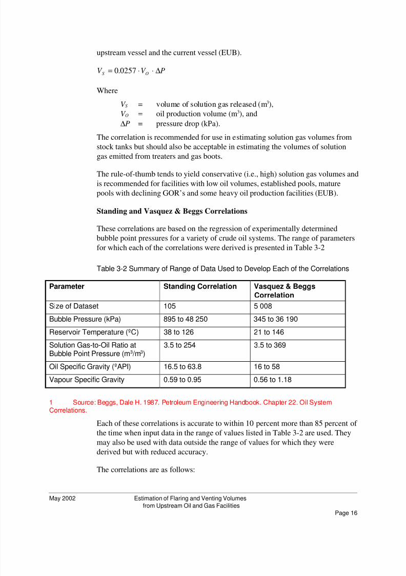
Standing and Vasquez & Beggs Correlations
These correlations are based on the regression of experimentally determined
bubble point pressures for a variety of crude oil systems. The range of parameters
for which each of the correlations were derived is presented in Table 3-2
Table 3-2 Summary of Range of Data Used to Develop Each of the Correlations
Parameter Standing Correlation Vasquez & Beggs
Correlation
Size of Dataset 105 5 008
Bubble Pressure (kPa) 895 to 48 250 345 to 36 190
Reservoir Temperature (ºC) 38 to 126 21 to 146
Solution Gas-to-Oil Ratio atBubble Point Pressure (m3 /m3)
3.5 to 254 3.5 to 369
Oil Specific Gravity (ºAPI) 16.5 to 63.8 16 to 58
Vapour Specific Gravity 0.59 to 0.95 0.56 to 1.18
1 Source: Beggs, Dale H. 1987. Petroleum Engineering Handbook. Chapter 22. Oil SystemCorrelations.
Each of these correlations is accurate to within 10 percent more than 85 percent of
the time when input data in the range of values listed in Table 3-2 are used. They
may also be used with data outside the range of values for which they were
derived but with reduced accuracy.
The correlations are as follows:
8/3/2019 Estimation of Flaring
http://slidepdf.com/reader/full/estimation-of-flaring 17/59Page 17
May 2002 Estimation of Flaring and Venting Volumes
from Upstream Oil and Gas Facilities
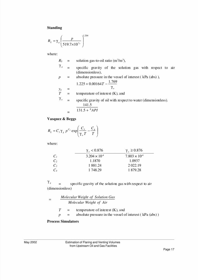
Standing
204.1
107.519
×=
g ygS
p R γ
where:
RS = solution gas-to-oil ratio (m3 /m3),
gγ = specific gravity of the solution gas with respect to air
(dimensionless),
p = absolute pressure in the vessel of interest ( kPa (abs) ),
yg = o
T γ
769.100164.0225.1 −+
T = temperature of interest (K), and
oγ = specific gravity of oil with respect to water (dimensionless).
= API o+5.131
5.141
Vasquez & Beggs
−=
T
C
T
C pC R
o
C
gS43
1 exp2
γ γ
where:
876.0<oγ 876.0≥oγ
C 1 3.204 × 10⁻⁴ 7.803 × 10⁻⁴
C 2 1.1870 1.0937
C 3 1 881.24 2 022.19
C 4 1 748.29 1 879.28
gγ = specific gravity of the solution gas with respect to air
(dimensionless)
Air of Weight Molecular
GasSolutionof Weight Molecular =
T = temperature of interest (K), and
p = absolute pressure in the vessel of interest ( kPa (abs) )
Process Simulators

8/3/2019 Estimation of Flaring
http://slidepdf.com/reader/full/estimation-of-flaring 18/59Page 18
May 2002 Estimation of Flaring and Venting Volumes
from Upstream Oil and Gas Facilities
Simulation of the process units may be performed with any one of a number of
commercially available process simulators. Table 3-3 provides a list of some
commercially available simulators and their suppliers.
The process data that are normally available at a facility and that may be useful in
simulating emulsion treaters and gas boots include:
composition of the inlet gas (on a dry basis),•composition of the final stabilized oil/condensate product from the stock •tanks,
gas flow rate off the inlet separator,•oil and water production rates to the stock tanks, and•operating temperatures and pressures of the various process vessels at the•facility.
The inlet production for the facility may be closely approximated by combining
the gas stream from the inlet separator with the stabilized hydrocarbon andproduced water streams at the inlet temperature and pressure. Having defined the
inlet production and knowing the operating temperature and pressure of the
downstream vessels, it is a simple matter to simulate the amount of gas vented or
flared from each of the process vessels.
If the composition and/or flow rate of the bulk process stream are not known at a
particular point, it is usually necessary to simulate all process units between the
inlet separator and the target unit.
Table 3-3 List of Commercially Available Process Simulation Packages
Package Vendor
Alpha Sim Alpha Sim Technology
5870 Hwy. 6 North, Suite 303
Houston, TX 77084
USA
ASPEN PLUS Aspen Technology Inc.
Ten Canal Park
Cambridge, Mass 02141-2200
USACHEMCAD III Chem Stations
2901 Wilcrest Drive, Suite 305
Houston, TX 77081
USA
8/3/2019 Estimation of Flaring
http://slidepdf.com/reader/full/estimation-of-flaring 19/59Page 19
May 2002 Estimation of Flaring and Venting Volumes
from Upstream Oil and Gas Facilities
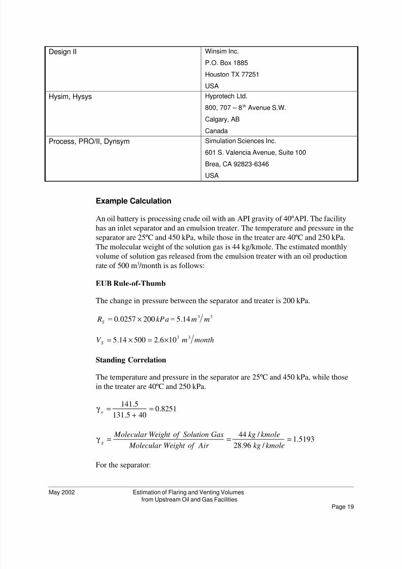
Design II Winsim Inc.
P.O. Box 1885
Houston TX 77251
USA
Hysim, Hysys Hyprotech Ltd.800, 707 – 8th Avenue S.W.
Calgary, AB
Canada
Process, PRO/II, Dynsym Simulation Sciences Inc.
601 S. Valencia Avenue, Suite 100
Brea, CA 92823-6346
USA
Example Calculation
An oil battery is processing crude oil with an API gravity of 40ºAPI. The facility
has an inlet separator and an emulsion treater. The temperature and pressure in the
separator are 25ºC and 450 kPa, while those in the treater are 40ºC and 250 kPa.
The molecular weight of the solution gas is 44 kg/kmole. The estimated monthly
volume of solution gas released from the emulsion treater with an oil production
rate of 500 m3 /month is as follows:
EUB Rule-of-Thumb
The change in pressure between the separator and treater is 200 kPa.
3314.52000257.0 mmkPa RS =×=
monthmV S33
106.250014.5 ×=×=
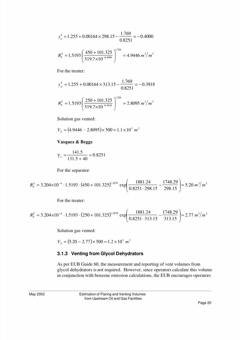
Standing Correlation
The temperature and pressure in the separator are 25ºC and 450 kPa, while those
in the treater are 40ºC and 250 kPa.
8251.0405.131
5.141 =+
=o
γ
5193.1 / 96.28
/ 44 ===kmolekg
kmolekg
Air of Weight Molecular
GasSolutionof Weight Molecular g
γ
For the separator:
8/3/2019 Estimation of Flaring
http://slidepdf.com/reader/full/estimation-of-flaring 20/59Page 20
May 2002 Estimation of Flaring and Venting Volumes
from Upstream Oil and Gas Facilities
4000.08251.0
769.115.29800164.0255.1 −=−×+=S
g y
33
204.1
4000.09446.4
107.519
325.1014505193.1 mm R
S
S =
×
+= −
For the treater:
3918.08251.0
769.115.31300164.0255.1 −=−×+=T
g y
33
204.1
3918.08095.2
107.519
325.1012505193.1 mm R
T
S =
×+
= −
Solution gas vented:
( ) 33101.15008095.29446.4 mV S ×=×−=
Vasquez & Beggs
8251.0405.131
5.141=
+=o
γ
For the separator:
( ) 331870.14 20.515.298
29.1748
15.2988251.0
24.1881exp325.1014505193.110204.3 mm R S
S =
−
⋅+⋅⋅×= −
For the treater:
( ) 331870.14 77.215.313
29.1748
15.3138251.0
24.1881exp325.1012505193.110204.3 mm RT
S =
−
⋅+⋅⋅×= −
Solution gas vented:
( ) 33102.150077.220.5 mV S ×=×−=
Venting from Glycol Dehydrators3.1.3
As per EUB Guide 60, the measurement and reporting of vent volumes from
glycol dehydrators is not required. However, since operators calculate this volume
in conjunction with benzene emission calculations, the EUB encourages operators
8/3/2019 Estimation of Flaring
http://slidepdf.com/reader/full/estimation-of-flaring 21/59Page 21
May 2002 Estimation of Flaring and Venting Volumes
from Upstream Oil and Gas Facilities
to report this volume. Glycol dehydration is a continuous liquid desiccant process
in which water or water vapour is removed from hydrocarbon streams by selective
absorption and the glycol is regenerated or reconcentrated by thermal desorption.
The use of triethylene glycol (TEG) is standard for dehydration of natural gas.
The primary causes of venting from a glycol dehydrator are secondaryabsorption/desorption by the TEG, entrainment of some gas from the contactor in
the rich TEG, and use of stripping gas in the reboiler.
Estimation Methods
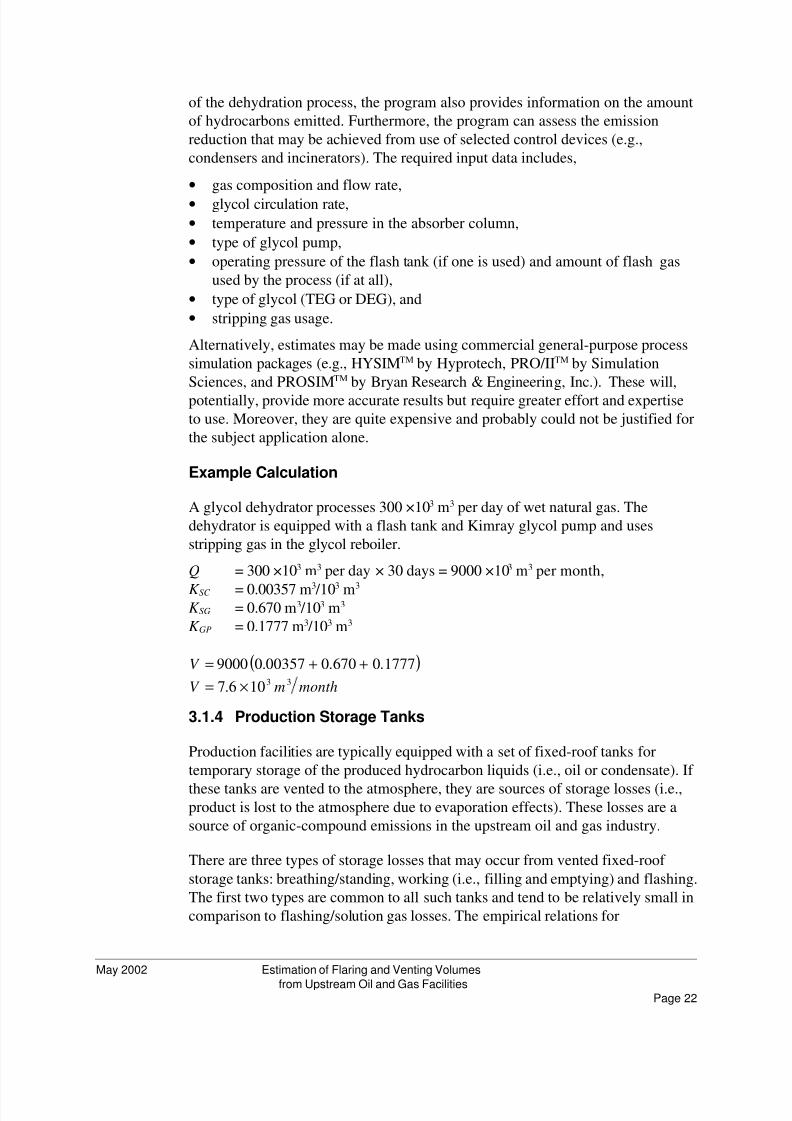
The simplest, but least accurate, method of estimating the quantity of natural gas
vented from the glycol regenerator still column is to use average emission factors.
These factors yield relatively accurate results on average. However, if the
dehydrator operating conditions differ significantly from the average then the
estimated vented volume will not reflect this. The volume of gas vented from a
glycol dehydrator still column may be estimated using the following relation:
( )GPSGSC K K K QV ++⋅=
where:
Q = gas throughput (103 m3),
K SC = still column off-gas factor (m3 /103 m3),
= 0.00357 if there is a flash tank,
= 0.1751 if there is no flash tank,
K SG = stripping gas factor (m3 /103 m3),
= 0.670 if stripping gas is used,= 0.000 if stripping gas is not used, and
K GP = Kimray pump factor (m3 /103 m3),
= 0.1777
The presented factors were derived by modeling typical glycol dehydration units
at gas production and processing facilities in the U.S. (Meyers, 1996).
Note that if an electric glycol pump is used, then the glycol pump factor is zero.
Similarly, if a gas driven glycol pump is used then the vent gas rate for the pump
should be estimated using the methods described in Section 3.1.5.
Perhaps the most convenient method of estimating methane emissions from aglycol dehydrator is to use the simulation program GRI-GLYCalc developed for,
and available at a nominal cost from, GTI (Thompson et al., 1994). GRI-GLYCalc
is primarily presented as a tool for estimating the amount benzene, toluene,
ethylbenzene and xylene (BTEX) emitted by a glycol dehydrator (significant
amounts of this material may be preferentially absorbed by the glycol and released
off the flash tank and still column). However, in performing a rigorous simulation
8/3/2019 Estimation of Flaring
http://slidepdf.com/reader/full/estimation-of-flaring 22/59Page 22
May 2002 Estimation of Flaring and Venting Volumes
from Upstream Oil and Gas Facilities
of the dehydration process, the program also provides information on the amount
of hydrocarbons emitted. Furthermore, the program can assess the emission
reduction that may be achieved from use of selected control devices (e.g.,
condensers and incinerators). The required input data includes,
gas composition and flow rate,•glycol circulation rate,•temperature and pressure in the absorber column,•type of glycol pump,•operating pressure of the flash tank (if one is used) and amount of flash gas•used by the process (if at all),
type of glycol (TEG or DEG), and•stripping gas usage.•
Alternatively, estimates may be made using commercial general-purpose process
simulation packages (e.g., HYSIMTM by Hyprotech, PRO/IITM by Simulation
Sciences, and PROSIMTM by Bryan Research & Engineering, Inc.). These will,
potentially, provide more accurate results but require greater effort and expertise
to use. Moreover, they are quite expensive and probably could not be justified for
the subject application alone.
Example Calculation
A glycol dehydrator processes 300 ×103 m3 per day of wet natural gas. The
dehydrator is equipped with a flash tank and Kimray glycol pump and uses
stripping gas in the glycol reboiler.
Q = 300 ×103 m3 per day × 30 days = 9000 ×103 m3 per month,
K SC = 0.00357 m3 /103 m3 K SG = 0.670 m3 /103 m3
K GP = 0.1777 m3 /103 m3
( )1777.0670.000357.09000 ++=V
monthmV 33106.7 ×=
Production Storage Tanks3.1.4
Production facilities are typically equipped with a set of fixed-roof tanks for
temporary storage of the produced hydrocarbon liquids (i.e., oil or condensate). If
these tanks are vented to the atmosphere, they are sources of storage losses (i.e.,product is lost to the atmosphere due to evaporation effects). These losses are a
source of organic-compound emissions in the upstream oil and gas industry.
There are three types of storage losses that may occur from vented fixed-roof
storage tanks: breathing/standing, working (i.e., filling and emptying) and flashing.
The first two types are common to all such tanks and tend to be relatively small in
comparison to flashing/solution gas losses. The empirical relations for
8/3/2019 Estimation of Flaring
http://slidepdf.com/reader/full/estimation-of-flaring 23/59Page 23
May 2002 Estimation of Flaring and Venting Volumes
from Upstream Oil and Gas Facilities
breathing/standing and working losses are well documented in the literature (API,
1991). Except in extraordinary circumstances, only flashing losses need to be
accounted for. As such, the focus of this section is flashing losses, which occur
when products with vapour pressures above atmospheric pressure are produced
into the tanks, as is the case at many oil and gas production facilities.
Estimation Methods
Produced hydrocarbon liquids at production facilities often contain a certain
amount of gas in solution; the amount is determined by the temperature and
pressure in the first vessel upstream of the stock tanks where the oil is in contact
with a hydrocarbon gas or vapour phase. When the product enters the tank, the
solution gas flashes/boils off causing a higher degree of saturation in the vapour
space than would be expected based on the vapour pressure of the weathered
product already in the tank.
If this process is examined in terms of vapour pressures, the produced liquid hasan initial value approximately equal to the operating pressure of the first upstream
vessel. When the product is placed in the stock tank its vapour pressure decreases
rapidly towards local barometric pressure, and then more slowly as the rate of
evaporation stabilizes. A weathered crude oil will typically have a vapour pressure
of 35 to 45 kPa at stock tank conditions.
The material that flashes from the product in going to a "stable" state is referred to
as solution gas. There are several approaches for estimating flashing losses from
storage tanks. These methods include the use of emission factors, estimation with
empirical correlations, and rigorous thermodynamic calculations using a process
simulator. The applicability of each of these methods is dependent upon thespecific conditions that exist at the production site.
As an alternative to estimation of emissions, solution gas emitted from the
production tank vent may be measured. To be useful, 24 hour test (similar to what
is required for GOR tests) must be conducted whereby both the solution gas and
oil production to the tank are measured. In practice, accurate measurement of
solution gas vented from a typical storage tank is difficult. Tanks commonly vent
gas not only from the central vent but also from the thief hatch and tank gauge
well. Sealing these openings to ensure that all gas exits through the flow meter is
difficult as the solution gas is typically saturated with condensable hydrocarbons
and water. As well, care must be taken not to overpressure the tank.
Empirical Correlations
The empirical correlations presented previously for estimating associated/solution
gas emissions may be used to estimate solution gas emissions from production
storage tanks. The correlations are:
8/3/2019 Estimation of Flaring
http://slidepdf.com/reader/full/estimation-of-flaring 24/59Page 24
May 2002 Estimation of Flaring and Venting Volumes
from Upstream Oil and Gas Facilities
EUB Rule-of-Thumb,•Standing Correlation, and•Vasquez & Beggs Correlation.•
Refer to Section 3.1.2 for a description of each of these correlations.
Rigorous Thermodynamic Simulations
The use of a process simulator potentially provides the most accurate estimate of
flashing/solution gas losses from production storage tanks. Analyses of both the
hydrocarbon liquid and solution gas streams as well as process temperatures and
pressures are generally required before a solution gas emission estimate can be
calculated. While, use of a process simulator requires substantially more effort
than correlations presented in Section 3.1.4.1.2, there may be circumstances where
it is the preferred method because the correlations or emission factors do not yield
acceptable results.
Estimation of solution gas emissions with a process simulator relies on the ability
to predict the liquid composition at the last vessel upstream of the storage tanks
using an equation of state. Flash calculations are then performed to determine the
quantity and composition of vapour released when the product is brought to stock
tank conditions. General process simulators such as Hysys, Prosim, Aspen, etc.
(see Table 6) are appropriate tools for estimating flashing losses. Alternately, a
more specialized package, E&P Tank (DB Robinson, 1997), may be used. An
added advantage of E&P Tank is that standing, working and flashing losses may
all be estimated using the same package.
E&P Tanks
E&P Tank is a software simulation package for estimating emissions from
hydrocarbon production tanks. The program was prepared by D.B. Robinson
Research Limited for American Petroleum Institute and Gas Research Institute
and is available from API. The model estimates production tank flashing losses
using thermodynamic principles and simulates working and standing losses by
one of several methods.
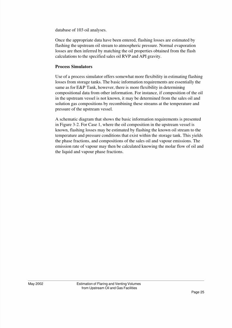
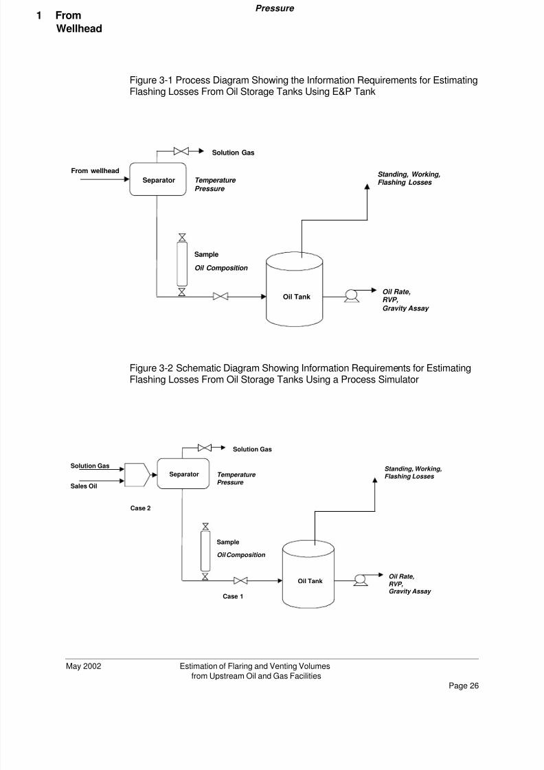
The storage tank to be simulated may be represented as shown in Figure 3-1. The
minimum information requirements for flashing loss calculations are:
upstream vessel temperature and pressure,•upstream vessel oil composition (at the temperature and pressure of the•upstream vessel) – a C1 to C10+ hydrocarbon analysis is required,
atmospheric pressure (or the pressure inside the storage tank),•RVP (Reid vapour pressure) of the sales oil, and•API gravity of the sales oil.•
If oil composition is not known, the program contains a fluid composition
8/3/2019 Estimation of Flaring
http://slidepdf.com/reader/full/estimation-of-flaring 25/59Page 25
May 2002 Estimation of Flaring and Venting Volumes
from Upstream Oil and Gas Facilities
database of 103 oil analyses.
Once the appropriate data have been entered, flashing losses are estimated by
flashing the upstream oil stream to atmospheric pressure. Normal evaporation
losses are then inferred by matching the oil properties obtained from the flash
calculations to the specified sales oil RVP and API gravity.
Process Simulators
Use of a process simulator offers somewhat more flexibility in estimating flashing
losses from storage tanks. The basic information requirements are essentially the
same as for E&P Tank, however, there is more flexibility in determining
compositional data from other information. For instance, if composition of the oil
in the upstream vessel is not known, it may be determined from the sales oil and
solution gas compositions by recombining these streams at the temperature and
pressure of the upstream vessel.
A schematic diagram that shows the basic information requirements is presented
in Figure 3-2. For Case 1, where the oil composition in the upstream vessel is
known, flashing losses may be estimated by flashing the known oil stream to the
temperature and pressure conditions that exist within the storage tank. This yields
the phase fractions, and compositions of the sales oil and vapour emissions. The
emission rate of vapour may then be calculated knowing the molar flow of oil and
the liquid and vapour phase fractions.
8/3/2019 Estimation of Flaring
http://slidepdf.com/reader/full/estimation-of-flaring 26/59Page 26
From wellhead
Separator
Solution Gas
Temperature
Pressure
Sample
Oil Composition
Oil TankOil Rate,RVP,
Gravity Assay
Standing, Working,Flashing Losses
Solution Gas
Separator
Solution Gas
Temperature
Pressure
Sample
Oil Composition
Oil TankOil Rate,
RVP,Gravity Assay
Standing, Working,Flashing Losses
Sales Oil
Case 2
Case 1
May 2002 Estimation of Flaring and Venting Volumes
from Upstream Oil and Gas Facilities
Figure 3-1 Process Diagram Showing the Information Requirements for EstimatingFlashing Losses From Oil Storage Tanks Using E&P Tank
Figure 3-2 Schematic Diagram Showing Information Requirements for EstimatingFlashing Losses From Oil Storage Tanks Using a Process Simulator
Pressure From1
Wellhead
8/3/2019 Estimation of Flaring
http://slidepdf.com/reader/full/estimation-of-flaring 27/59Page 27
May 2002 Estimation of Flaring and Venting Volumes
from Upstream Oil and Gas Facilities
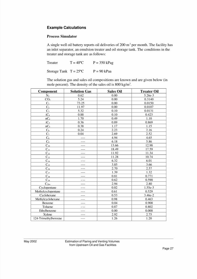
Example Calculations
Process Simulator
A single well oil battery reports oil deliveries of 200 m 3 per month. The facility has
an inlet separator, an emulsion treater and oil storage tank. The conditions in thetreater and storage tank are as follows:
Treater T = 40ºC P = 350 kPag
Storage Tank T = 25ºC P = 90 kPaa
The solution gas and sales oil compositions are known and are given below (in
mole percent). The density of the sales oil is 800 kg/m3.
Component Solution Gas Sales Oil Treater OilN2 0.62 0.00 5.26e-3
CO2 5.24 0.00 0.3140
C1 73.25 0.00 0.0150C2 11.97 0.00 0.0107
C3 5.32 0.10 0.0131iC4 0.88 0.10 0.423nC4 1.70 0.49 1.10
iC5 0.36 0.89 0.869nC5 0.38 1.17 1.15
C6 0.24 2.23 2.16C7 0.04 2.69 2.52
C8 ---- 4.94 4.65C9 ---- 6.18 5.86
C10 ---- 13.66 12.98C11 ---- 18.49 17.59C12 ---- 11.92 11.34
C13 ---- 11.28 10.74C14 ---- 6.32 6.01
C15 ---- 3.85 3.66C16 ---- 2.70 2.57
C17 ---- 1.39 1.32C18 ---- 0.81 0.771C19 ---- 0.62 0.590
C20+ ---- 2.94 2.80Cyclopentane ---- 0.02 1.55e-3
Methylcyclopentane ---- 0.61 0.529
Cyclohexane ---- 0.53 3.46e-2Methylcyclohexane ---- 0.98 0.463
Benzene ---- 0.04 0.900Toluene ---- 0.87 0.802
Ethylbenzene ---- 0.00 0.000Xylene ---- 2.92 2.75
124-Trimethylbenzene ---- 1.26 1.20
8/3/2019 Estimation of Flaring
http://slidepdf.com/reader/full/estimation-of-flaring 28/59Page 28
May 2002 Estimation of Flaring and Venting Volumes
from Upstream Oil and Gas Facilities
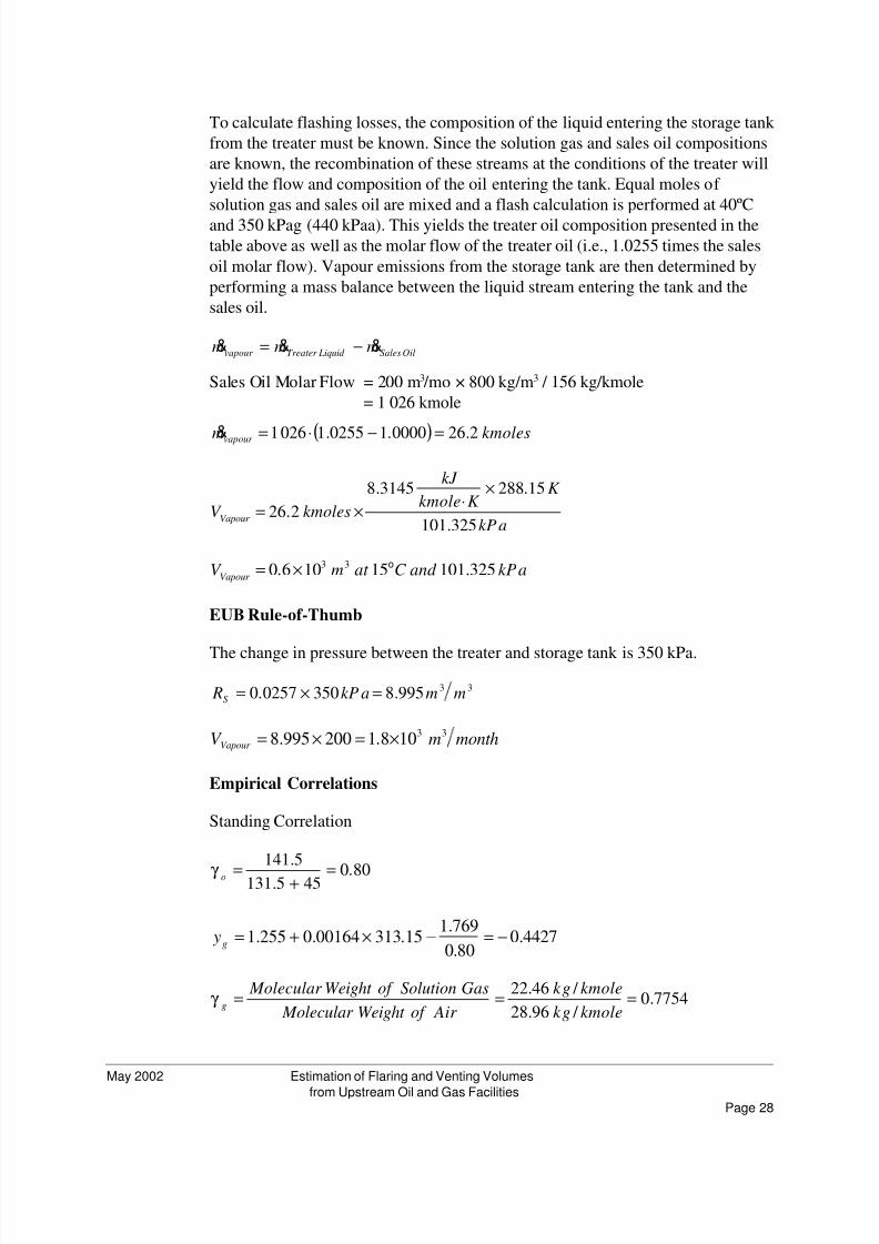
To calculate flashing losses, the composition of the liquid entering the storage tank
from the treater must be known. Since the solution gas and sales oil compositions
are known, the recombination of these streams at the conditions of the treater will
yield the flow and composition of the oil entering the tank. Equal moles of
solution gas and sales oil are mixed and a flash calculation is performed at 40ºC
and 350 kPag (440 kPaa). This yields the treater oil composition presented in the
table above as well as the molar flow of the treater oil (i.e., 1.0255 times the sales
oil molar flow). Vapour emissions from the storage tank are then determined by
performing a mass balance between the liquid stream entering the tank and the
sales oil.
OilSales Liquid Treater vapour mmm &&& −=
Sales Oil Molar Flow = 200 m3 /mo × 800 kg/m3 / 156 kg/kmole
= 1 026 kmole
( ) kmolesmvapour 2.260000.10255.10261 =−⋅=&
kPa
K K kmole
kJ
kmolesV Vapour
325.101
15.2883145.8
2.26
×⋅×=
kPaand C at mV Vapour
325.10115106.0 33 o×=
EUB Rule-of-Thumb
The change in pressure between the treater and storage tank is 350 kPa.
33995.83500257.0 mmkPa RS =×=
monthmV Vapour
33108.1200995.8 ×=×=
Empirical Correlations
Standing Correlation
80.0455.131
5.141
=+=oγ
4427.080.0
769.115.31300164.0255.1 −=−×+=
g y
7754.0 / 96.28
/ 46.22 ===kmolekg
kmolekg
Air of Weight Molecular
GasSolutionof Weight Molecular g
γ
8/3/2019 Estimation of Flaring
http://slidepdf.com/reader/full/estimation-of-flaring 29/59Page 29
May 2002 Estimation of Flaring and Venting Volumes
from Upstream Oil and Gas Facilities
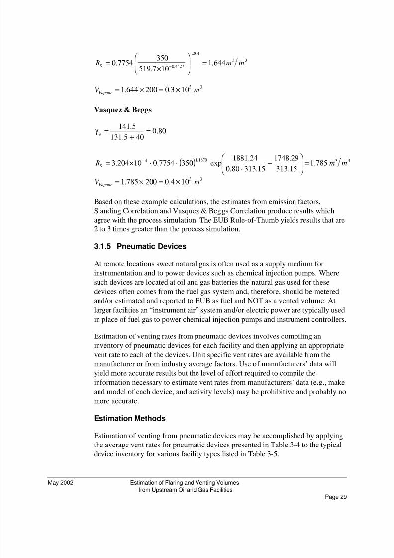
33
204.1
4427.0644.1
107.519
3507754.0 mm RS =
×
= −
33103.0200644.1 mV Vapour ×=×=
Vasquez & Beggs
80.0405.131
5.141 =+
=o
γ
( ) 331870.14 785.115.313
29.1748
15.31380.0
24.1881exp3507754.010204.3 mm RS =
−
⋅⋅⋅×= −
33104.0200785.1 mV Vapour ×=×=
Based on these example calculations, the estimates from emission factors,
Standing Correlation and Vasquez & Beggs Correlation produce results which
agree with the process simulation. The EUB Rule-of-Thumb yields results that are
2 to 3 times greater than the process simulation.
Pneumatic Devices3.1.5
At remote locations sweet natural gas is often used as a supply medium for
instrumentation and to power devices such as chemical injection pumps. Where
such devices are located at oil and gas batteries the natural gas used for these
devices often comes from the fuel gas system and, therefore, should be meteredand/or estimated and reported to EUB as fuel and NOT as a vented volume. At
larger facilities an “instrument air” system and/or electric power are typically used
in place of fuel gas to power chemical injection pumps and instrument controllers.
Estimation of venting rates from pneumatic devices involves compiling an
inventory of pneumatic devices for each facility and then applying an appropriate
vent rate to each of the devices. Unit specific vent rates are available from the
manufacturer or from industry average factors. Use of manufacturers’ data will
yield more accurate results but the level of effort required to compile the
information necessary to estimate vent rates from manufacturers’ data (e.g., make
and model of each device, and activity levels) may be prohibitive and probably nomore accurate.
Estimation Methods
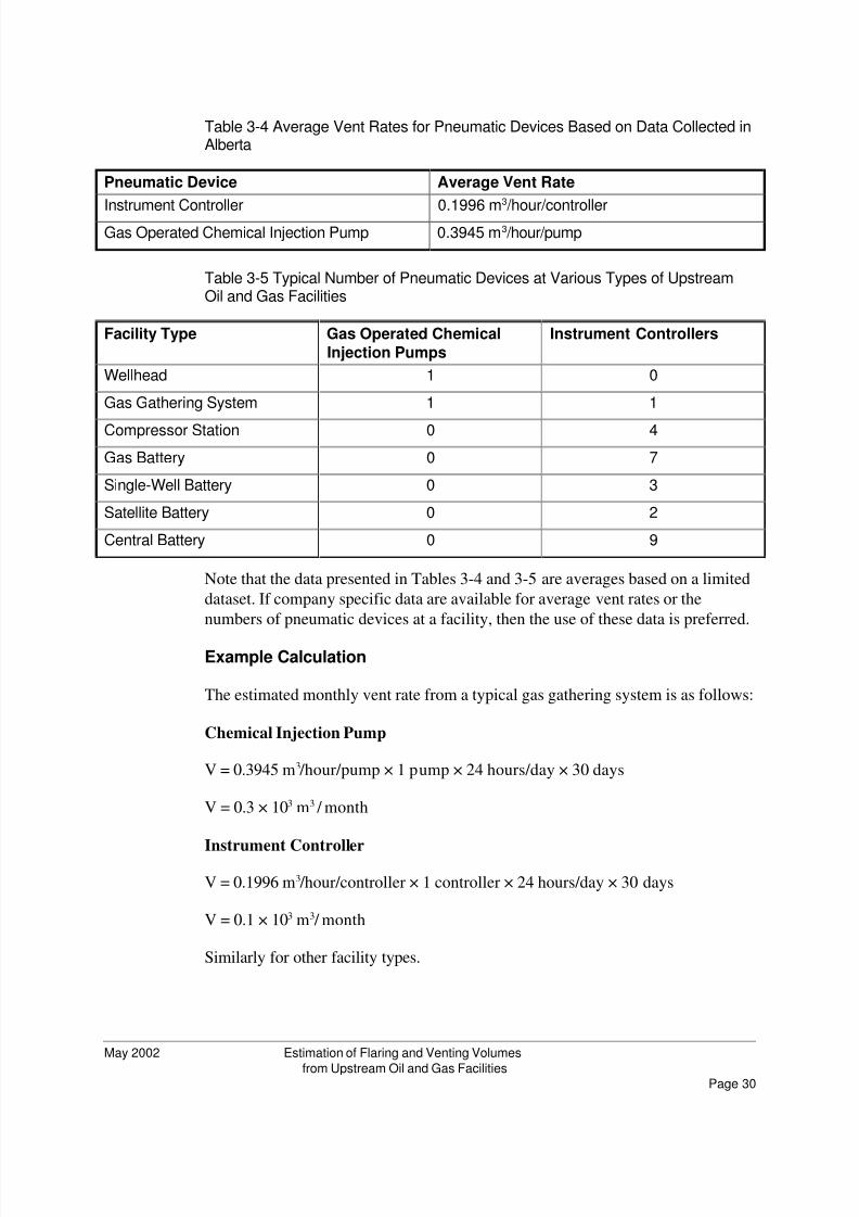
Estimation of venting from pneumatic devices may be accomplished by applying
the average vent rates for pneumatic devices presented in Table 3-4 to the typical
device inventory for various facility types listed in Table 3-5.
8/3/2019 Estimation of Flaring
http://slidepdf.com/reader/full/estimation-of-flaring 30/59Page 30
May 2002 Estimation of Flaring and Venting Volumes
from Upstream Oil and Gas Facilities
Table 3-4 Average Vent Rates for Pneumatic Devices Based on Data Collected inAlberta
Pneumatic Device Average Vent Rate
Instrument Controller 0.1996 m
3
/hour/controllerGas Operated Chemical Injection Pump 0.3945 m3 /hour/pump
Table 3-5 Typical Number of Pneumatic Devices at Various Types of UpstreamOil and Gas Facilities
Facility Type Gas Operated Chemical
Injection Pumps
Instrument Controllers
Wellhead 1 0
Gas Gathering System 1 1
Compressor Station 0 4
Gas Battery 0 7
Single-Well Battery 0 3
Satellite Battery 0 2
Central Battery 0 9
Note that the data presented in Tables 3-4 and 3-5 are averages based on a limited
dataset. If company specific data are available for average vent rates or the
numbers of pneumatic devices at a facility, then the use of these data is preferred.
Example Calculation
The estimated monthly vent rate from a typical gas gathering system is as follows:
Chemical Injection Pump
V = 0.3945 m3 /hour/pump × 1 pump × 24 hours/day × 30 days
V = 0.3 × 10³ m3 / month
Instrument Controller
V = 0.1996 m3 /hour/controller × 1 controller × 24 hours/day × 30 days
V = 0.1 × 10³ m3 / month
Similarly for other facility types.
8/3/2019 Estimation of Flaring
http://slidepdf.com/reader/full/estimation-of-flaring 31/59Page 31
May 2002 Estimation of Flaring and Venting Volumes
from Upstream Oil and Gas Facilities
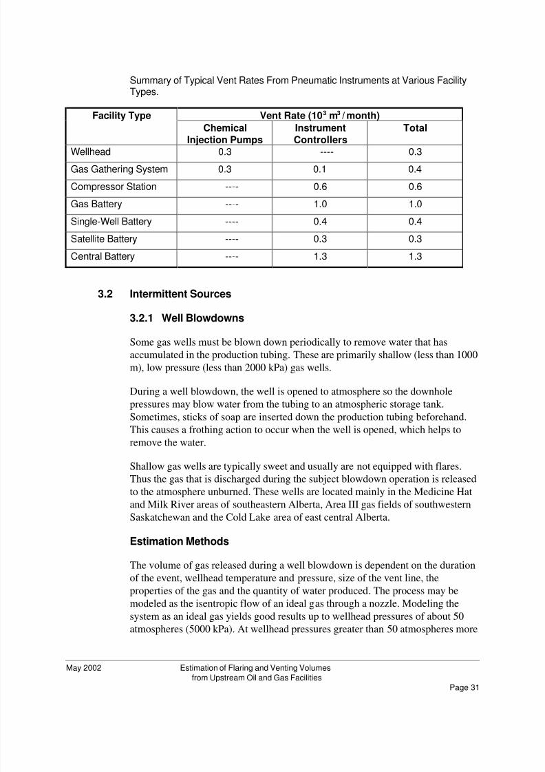
Summary of Typical Vent Rates From Pneumatic Instruments at Various FacilityTypes.
Facility Type Vent Rate (103 m3 / month)
Chemical
Injection Pumps
Instrument
Controllers
Total
Wellhead 0.3 ---- 0.3
Gas Gathering System 0.3 0.1 0.4
Compressor Station ---- 0.6 0.6
Gas Battery ---- 1.0 1.0
Single-Well Battery ---- 0.4 0.4
Satellite Battery ---- 0.3 0.3
Central Battery ---- 1.3 1.3
Intermittent Sources3.2
Well Blowdowns3.2.1
Some gas wells must be blown down periodically to remove water that has
accumulated in the production tubing. These are primarily shallow (less than 1000
m), low pressure (less than 2000 kPa) gas wells.
During a well blowdown, the well is opened to atmosphere so the downhole
pressures may blow water from the tubing to an atmospheric storage tank.Sometimes, sticks of soap are inserted down the production tubing beforehand.
This causes a frothing action to occur when the well is opened, which helps to
remove the water.
Shallow gas wells are typically sweet and usually are not equipped with flares.
Thus the gas that is discharged during the subject blowdown operation is released
to the atmosphere unburned. These wells are located mainly in the Medicine Hat
and Milk River areas of southeastern Alberta, Area III gas fields of southwestern
Saskatchewan and the Cold Lake area of east central Alberta.
Estimation Methods
The volume of gas released during a well blowdown is dependent on the duration
of the event, wellhead temperature and pressure, size of the vent line, the
properties of the gas and the quantity of water produced. The process may be
modeled as the isentropic flow of an ideal gas through a nozzle. Modeling the
system as an ideal gas yields good results up to wellhead pressures of about 50
atmospheres (5000 kPa). At wellhead pressures greater than 50 atmospheres more
8/3/2019 Estimation of Flaring
http://slidepdf.com/reader/full/estimation-of-flaring 32/59Page 32
May 2002 Estimation of Flaring and Venting Volumes
from Upstream Oil and Gas Facilities
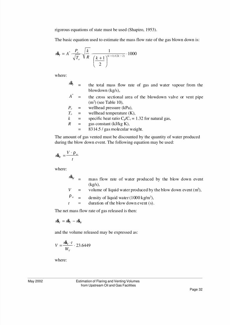
rigorous equations of state must be used (Shapiro, 1953).
The basic equation used to estimate the mass flow rate of the gas blown down is:
1000
2
1
1
)22 /()1(
* ⋅
+⋅⋅⋅=
−+ k k o
o
T
k R
k
T
P Am&
where:
T m& = the total mass flow rate of gas and water vapour from the
blowdown (kg/s),* A = the cross sectional area of the blowdown valve or vent pipe
(m2) (see Table 10),
Po = wellhead pressure (kPa),
T o = wellhead temperature (K),k = specific heat ratio Cp /Cv = 1.32 for natural gas,
R = gas constant (kJ/kg K),
= 8314.5 / gas molecular weight.
The amount of gas vented must be discounted by the quantity of water produced
during the blow down event. The following equation may be used:
t
V m w
W
ρ⋅=&
where:W m&
= mass flow rate of water produced by the blow down event
(kg/s),
V = volume of liquid water produced by the blow down event (m3),
wρ= density of liquid water (1000 kg/m3),
t = duration of the blow down event (s).
The net mass flow rate of gas released is then:
W T V mmm &&& −=
and the volume released may be expressed as:
6449.23⋅⋅
=V
V
W
t mV
&
where:
8/3/2019 Estimation of Flaring
http://slidepdf.com/reader/full/estimation-of-flaring 33/59Page 33
May 2002 Estimation of Flaring and Venting Volumes
from Upstream Oil and Gas Facilities
V = volume of gas released (m3),
W V = molecular weight of the vapour released (kg/kmole), and
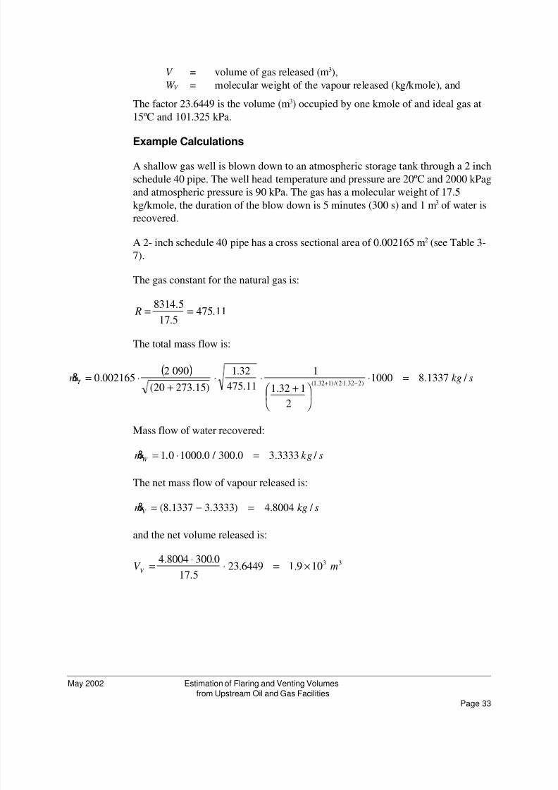
The factor 23.6449 is the volume (m3) occupied by one kmole of and ideal gas at
15ºC and 101.325 kPa.
Example Calculations
A shallow gas well is blown down to an atmospheric storage tank through a 2 inch
schedule 40 pipe. The well head temperature and pressure are 20ºC and 2000 kPag
and atmospheric pressure is 90 kPa. The gas has a molecular weight of 17.5
kg/kmole, the duration of the blow down is 5 minutes (300 s) and 1 m3 of water is
recovered.
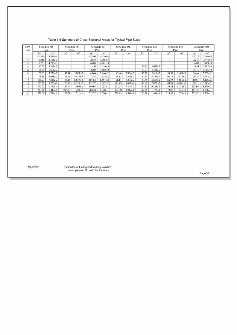
A 2- inch schedule 40 pipe has a cross sectional area of 0.002165 m2 (see Table 3-
7).
The gas constant for the natural gas is:
11.4755.17
5.8314== R
The total mass flow is:
( )skgmT / 1337.81000
2
132.1
1
11.475
32.1
)15.27320(
0902002165.0
)232.12 /()132.1(=⋅
+
⋅⋅+
⋅= −⋅+&
Mass flow of water recovered:
skgmW / 3333.30.300 / 0.10000.1 =⋅=&
The net mass flow of vapour released is:
skgmV / 8004.4)3333.31337.8( =−=&
and the net volume released is:
33109.16449.235.17
0.3008004.4mV
V ×=⋅⋅=
8/3/2019 Estimation of Flaring
http://slidepdf.com/reader/full/estimation-of-flaring 34/59
Page 34
May 2002 Estimation of Flaring and Venting Volumes
from Upstream Oil and Gas Facilities
Table 3-6 Summary of Cross-Sectional Areas for Typical Pipe Sizes
NPSSize
Schedule 40Pipe
Schedule 60Pipe
Schedule 80Pipe
Schedule 100Pipe
Schedule 120Pipe
Schedule 140Pipe
Schedule 160Pipe
in2 m2 in2 m2 in2 m2 in2 m2 in2 m2 in2 m2 in2 m2
1 0.8640 5.574e-4 0.7190 4.639e-4 0.5217 3.366e-4
2 3.355 2.165e-3 2.953 1.905e-3 2.241 1.446e-3
3 7.393 4.770e-3 6.605 4.261e-3 5.408 3.489e-3
4 12.73 8.213e-3 11.50 7.419e-3 10.31 6.652e-3 9.28 5.987e-3
6 28.89 1.864e-2 26.07 1.682e-2 23.77 1.534e-2 21.15 1.365e-2
8 50.03 3.228e-2 47.94 3.093e-2 45.66 2.946e-2 43.46 2.804e-2 40.59 2.619e-2 38.50 2.484e-2 36.46 2.352e-2
10 78.86 5.088e-2 74.66 4.817e-2 71.84 4.635e-2 68.13 4.395e-2 64.53 4.163e-2 60.13 3.879e-2 56.75 3.661e-2
12 111.93 7.221e-2 106.16 6.849e-2 101.64 6.557e-2 96.14 6.203e-2 90.76 5.855e-2 86.59 5.586e-2 80.53 5.195e-2
14 135.28 8.728e-2 128.96 8.320e-2 122.72 7.917e-2 115.49 7.451e-2 109.62 7.072e-2 103.87 6.701e-2 98.31 6.343e-2
16 176.72 1.140e-1 169.44 1.093e-1 160.92 1.038e-1 152.58 9.844e-2 144.50 9.323e-2 135.28 8.728e-2 128.96 8.320e-2
18 223.68 1.443e-1 213.83 1.380e-1 204.24 1.318e-1 193.30 1.247e-1 182.66 1.178e-1 173.80 1.121e-1 163.72 1.056e-1
20 278.00 1.794e-1 265.21 1.711e-1 252.72 1.630e-1 238.83 1.541e-1 226.98 1.464e-1 213.82 1.379e-1 202.67 1.308e-1
8/3/2019 Estimation of Flaring
http://slidepdf.com/reader/full/estimation-of-flaring 35/59Page 35
May 2002 Estimation of Flaring and Venting Volumes
from Upstream Oil and Gas Facilities
Accidental Releases3.2.2
Accidental releases are releases that occur as a result of accidents, human error
and extraordinary equipment failures. These releases are not part of normal
operational or maintenance activities and exclude such releases as, for example,
relief valve emissions.
The most significant types of natural gas emissions in this category are those from
pipeline ruptures, well blowouts, surface casing vent blows and gas migration to
the surface. For certain types of sources, such as surface casing vent blows and
gas migration around the outside of the casing, measurement of the vented gas is
preferred.
Estimation Methods
Each of the types of accidental losses is delineated below, along with some
methods to estimate the emissions.
Pipeline Ruptures
A pipeline rupture may be approximated using the estimation methods described
in the well blowdown and pressure vessel blowdown sections (Sections 3.2.1 and
3.2.4, respectively). The rupture is essentially a blowdown from an infinite
reservoir from the time of the rupture until the isolation valves on the pipeline are
closed. After that point it is simply the blowdown of a section of pipe from some
initial pressure to atmospheric pressure.
Well Blowouts
A well blowout is an uncontrolled release of natural gas caused by a catastrophic
failure of some part of a wellhead. A blowout may be a complex system to model,
therefore, it is preferred to estimate the volume of gas released from a blowdown
based on gas well deliverability tests or absolute open flow potential (AOFP) tests.
These tests are described in detail in EUB Guide 40 (Pressure and Deliverability
Testing Oil and Gas Wells).
Surface-Casing Vent Flows
The surface casing is a steel liner used to protect the integrity of the well bore asthe hole is being drilled and to prevent contamination of any aquifers that may be
a source of potable water. It is installed during the initial stages of the drilling
program and is cemented in place by pumping cement down the centre of the pipe
and forcing it to return up around the outside wall. The depth to which the surface
casing extends is determined by regulations and the geological conditions at the
site (surface casing may not be required on some shallow wells). When the well is
8/3/2019 Estimation of Flaring
http://slidepdf.com/reader/full/estimation-of-flaring 36/59Page 36
May 2002 Estimation of Flaring and Venting Volumes
from Upstream Oil and Gas Facilities
completed, the production casing is run down the centre of the surface casing and
cemented in place in a similar manner. The surface casing vent valve is left open to
allow for constant monitoring of the annular space between the production casing
and the surface casing. In this manner, any gas or other fluids that may flow out
from the surrounding formation or up from below can flow into the casing
annulus rather than migrate up around the outside of the surface casing andpossibly contaminate aquifers above.
If a vent blow occurs, the exact cause of the flow may be difficult to determine
and the required repairs are often costly. The fluid emitted from a vent blow may
consist of gas, oil, fresh water, salt water or drilling mud. Some vent blows
eventually die out. In some cases the vent flow is produced, in others either it is
vented/flared or the vent is blocked-in and pressure is allowed to build-up in the
casing. One piece of information that can be useful in determining the nature of
the vent flow is the surface casing vent shut-in pressure. By closing the surface
casing vent valve and monitoring the shut-in pressure using a suitably accurate
gauge, this can be easily determined.
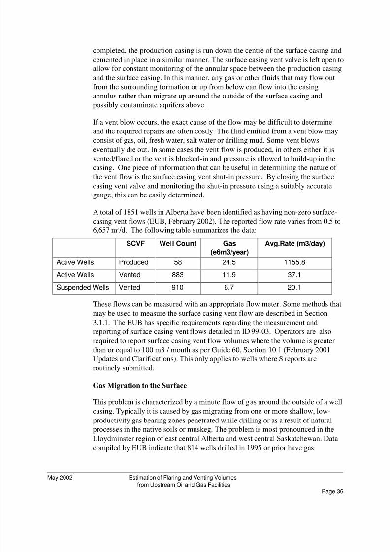
A total of 1851 wells in Alberta have been identified as having non-zero surface-
casing vent flows (EUB, February 2002). The reported flow rate varies from 0.5 to
6,657 m3 /d. The following table summarizes the data:
SCVF Well Count Gas
(e6m3/year)
Avg.Rate (m3/day)
Active Wells Produced 58 24.5 1155.8
Active Wells Vented 883 11.9 37.1
Suspended Wells Vented 910 6.7 20.1
These flows can be measured with an appropriate flow meter. Some methods that
may be used to measure the surface casing vent flow are described in Section
3.1.1. The EUB has specific requirements regarding the measurement and
reporting of surface casing vent flows detailed in ID 99-03. Operators are also
required to report surface casing vent flow volumes where the volume is greater
than or equal to 100 m3 / month as per Guide 60, Section 10.1 (February 2001
Updates and Clarifications). This only applies to wells where S reports are
routinely submitted.
Gas Migration to the Surface
This problem is characterized by a minute flow of gas around the outside of a well
casing. Typically it is caused by gas migrating from one or more shallow, low-
productivity gas bearing zones penetrated while drilling or as a result of natural
processes in the native soils or muskeg. The problem is most pronounced in the
Lloydminster region of east central Alberta and west central Saskatchewan. Data
compiled by EUB indicate that 814 wells drilled in 1995 or prior have gas
8/3/2019 Estimation of Flaring
http://slidepdf.com/reader/full/estimation-of-flaring 37/59Page 37
May 2002 Estimation of Flaring and Venting Volumes
from Upstream Oil and Gas Facilities
migration problems.
Estimation of the volume of vented gas requires measurement of the hydrocarbon
flux rate in the region of the wellhead. One method of making these
measurements is through the use of an isolation flux chamber. Tests of this nature
have been conducted by Husky Oil Operations (Erno and Schmitz, 1996 andSchmitz et al., 1996). Based on the data presented in these papers, the average
vent rate for wells with gas migration problems is 3.85 m3 /d per well. As with
surface casing vent flows, the EUB has mandated specific requirements for testing
and reporting gas migration in EUB ID 99-03. Operators are required to report gas
migration volumes if greater than or equal to 100 m3/month as per Guide 60,
Section 10.2 (February 2001 Updates and Clarifications). As with surface casing
vent flows, this only applies to wells where S Reports are routinely submitted.
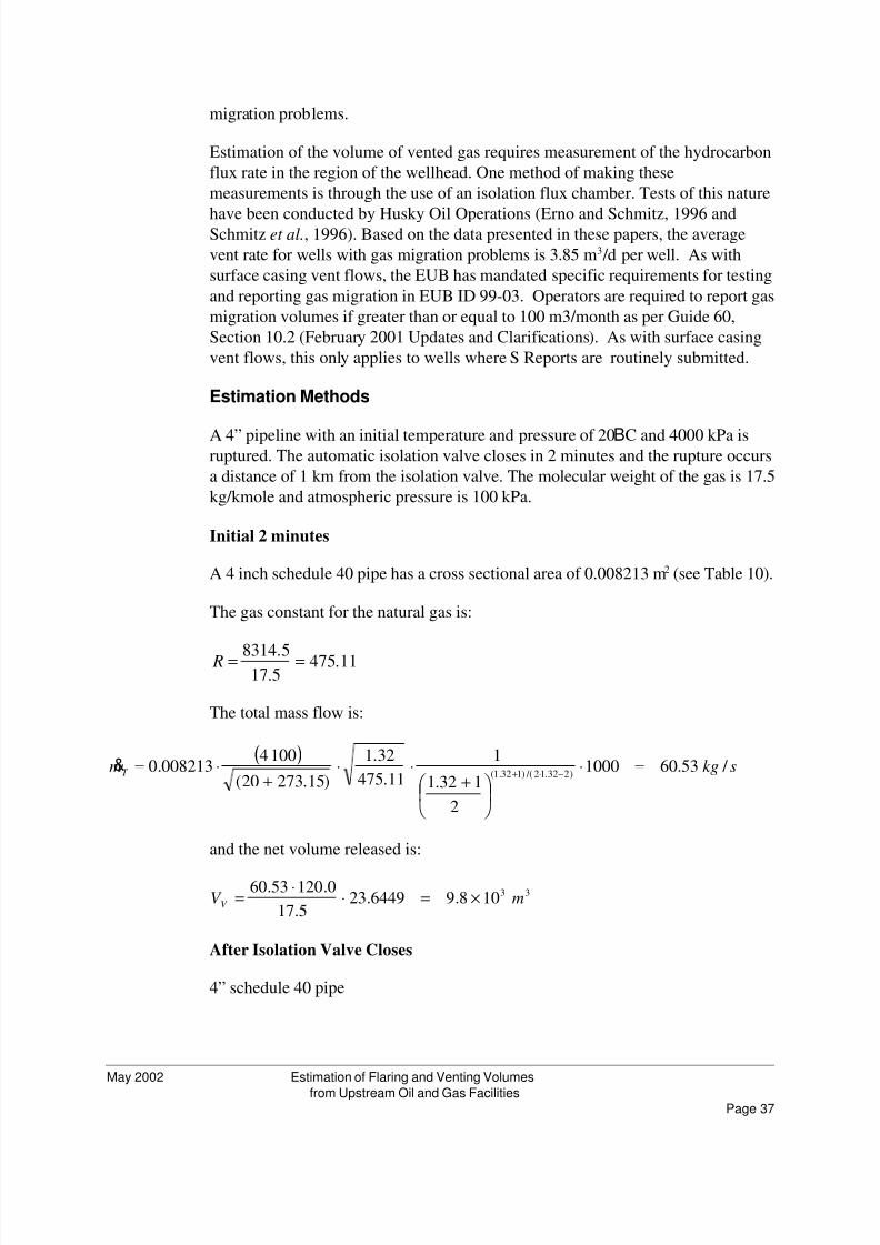
Estimation Methods
A 4” pipeline with an initial temperature and pressure of 20BC and 4000 kPa isruptured. The automatic isolation valve closes in 2 minutes and the rupture occurs
a distance of 1 km from the isolation valve. The molecular weight of the gas is 17.5
kg/kmole and atmospheric pressure is 100 kPa.
Initial 2 minutes
A 4 inch schedule 40 pipe has a cross sectional area of 0.008213 m2 (see Table 10).
The gas constant for the natural gas is:
11.4755.175.8314 == R
The total mass flow is:
( )skgmT / 53.601000
2
132.1
1
11.475
32.1
)15.27320(
1004008213.0
)232.12 /()132.1(=⋅
+
⋅⋅+
⋅= −⋅+&
and the net volume released is:
33108.96449.235.17
0.12053.60mV V ×=⋅
⋅=
After Isolation Valve Closes
4” schedule 40 pipe
8/3/2019 Estimation of Flaring
http://slidepdf.com/reader/full/estimation-of-flaring 38/59Page 38
May 2002 Estimation of Flaring and Venting Volumes
from Upstream Oil and Gas Facilities
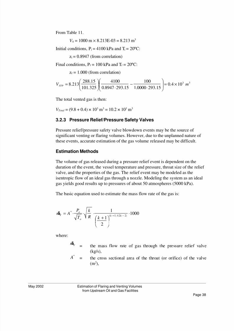
From Table 11.
V A = 1000 m × 8.213E-03 = 8.213 m3
Initial conditions, Pi = 4100 kPa and Ti = 20°C:
zi = 0.8947 (from correlation)Final conditions, Pf = 100 kPa and Tf = 20°C:
zf = 1.000 (from correlation)
33104.015.2930000.1
100
15.2938947.0
4100
325.101
15.288213.8 mV STP ×=
⋅
−⋅
=
The total vented gas is then:
V Total = (9.8 + 0.4) × 103 m3 = 10.2 × 10³ m3
Pressure Relief/Pressure Safety Valves3.2.3
Pressure relief/pressure safety valve blowdown events may be the source of
significant venting or flaring volumes. However, due to the unplanned nature of
these events, accurate estimation of the gas volume released may be difficult.
Estimation Methods
The volume of gas released during a pressure relief event is dependent on the
duration of the event, the vessel temperature and pressure, throat size of the relief
valve, and the properties of the gas. The relief event may be modeled as theisentropic flow of an ideal gas through a nozzle. Modeling the system as an ideal
gas yields good results up to pressures of about 50 atmospheres (5000 kPa).
The basic equation used to estimate the mass flow rate of the gas is:
1000
2
1
1)22 /()1(
* ⋅
+⋅⋅⋅= −+ k k
o
o
V
k R
k
T
P Am&
where:
V m&= the mass flow rate of gas through the pressure relief valve
(kg/s),* A = the cross sectional area of the throat (or orifice) of the valve
(m2),

8/3/2019 Estimation of Flaring
http://slidepdf.com/reader/full/estimation-of-flaring 39/59Page 39
May 2002 Estimation of Flaring and Venting Volumes
from Upstream Oil and Gas Facilities
oP = pressure relief valve set point (kPa),
T o = vessel temperature (K),
k = specific heat ratio Cp /Cv = 1.32 for natural gas, and
R = gas constant (kJ/kg K),
= 8314.5 / gas molecular weight.
The volume released may be expressed as:
6449.23⋅⋅
=V
V
W
t mV
&
where:
V = volume of gas released (m3),
W V = molecular weight of the vapour released (kg/kmole), and
The factor 23.6449 is the volume (m3) occupied by one kmole of and ideal gas at
15ºC and 101.325 kPa.
The orifice cross-sectional area is dependent on the valve size, the inlet and back
pressures, and inlet temperature. Therefore, there is no simple relationship
between the size of the pressure relief valve and the orifice cross-sectional area
and the orifice area must be determined from manufacturers’ data for each
individual application.
Example Calculation
A vessel has a 3 inch pressure relief valve (throat area = 0.00477 m 2) set at 3000
kPag. An overpressure event causes the valve to open for a duration of 1 minute(60 seconds). The molecular weight of the gas in the vessel is 17.5 kg/kmole, the
vessel temperature is 50ºC and atmospheric pressure is 100 kPa.
The gas constant for the natural gas is:
11.4755.17
5.8314== R
The mass flow rate through the pressure relief valve is:
( )skgmV / 3167.251000
2
132.1
1
11.475
32.1
)15.27350(
100300477.0
)232.12 /()132.1(=⋅
+
⋅⋅+
⋅= −⋅+&
The volume of gas released is:
8/3/2019 Estimation of Flaring
http://slidepdf.com/reader/full/estimation-of-flaring 40/59Page 40
May 2002 Estimation of Flaring and Venting Volumes
from Upstream Oil and Gas Facilities
33101.26449.235.17
0.603167.25mV
V ×=⋅
⋅=
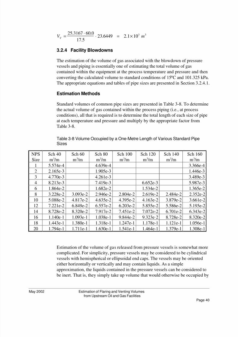
Facility Blowdowns3.2.4
The estimation of the volume of gas associated with the blowdown of pressurevessels and piping is essentially one of estimating the total volume of gas
contained within the equipment at the process temperature and pressure and then
converting the calculated volume to standard conditions of 15°C and 101.325 kPa.
The appropriate equations and tables of pipe sizes are presented in Section 3.2.4.1.
Estimation Methods
Standard volumes of common pipe sizes are presented in Table 3-8. To determine
the actual volume of gas contained within the process piping (i.e., at process
conditions), all that is required is to determine the total length of each size of pipe
at each temperature and pressure and multiply by the appropriate factor from
Table 3-8.
Table 3-8 Volume Occupied by a One-Metre Length of Various Standard PipeSizes
NPS
Size
Sch 40
m3 /m
Sch 60
m3 /m
Sch 80
m3 /m
Sch 100
m3 /m
Sch 120
m3 /m
Sch 140
m3 /m
Sch 160
m3 /m
1 5.574e-4 4.639e-4 3.366e-4
2 2.165e-3 1.905e-3 1.446e-3
3 4.770e-3 4.261e-3 3.489e-34 8.213e-3 7.419e-3 6.652e-3 5.987e-3
6 1.864e-2 1.682e-2 1.534e-2 1.365e-2
8 3.228e-2 3.093e-2 2.946e-2 2.804e-2 2.619e-2 2.484e-2 2.352e-2
10 5.088e-2 4.817e-2 4.635e-2 4.395e-2 4.163e-2 3.879e-2 3.661e-2
12 7.221e-2 6.849e-2 6.557e-2 6.203e-2 5.855e-2 5.586e-2 5.195e-2
14 8.728e-2 8.320e-2 7.917e-2 7.451e-2 7.072e-2 6.701e-2 6.343e-2
16 1.140e-1 1.093e-1 1.038e-1 9.844e-2 9.323e-2 8.728e-2 8.320e-2
18 1.443e-1 1.380e-1 1.318e-1 1.247e-1 1.178e-1 1.121e-1 1.056e-1
20 1.794e-1 1.711e-1 1.630e-1 1.541e-1 1.464e-1 1.379e-1 1.308e-1
Estimation of the volume of gas released from pressure vessels is somewhat more
complicated. For simplicity, pressure vessels may be considered to be cylindrical
vessels with hemispherical or ellipsoidal end caps. The vessels may be oriented
either horizontally or vertically and may contain liquids. As a simple
approximation, the liquids contained in the pressure vessels can be considered to
be inert. That is, they simply take up volume that would otherwise be occupied by
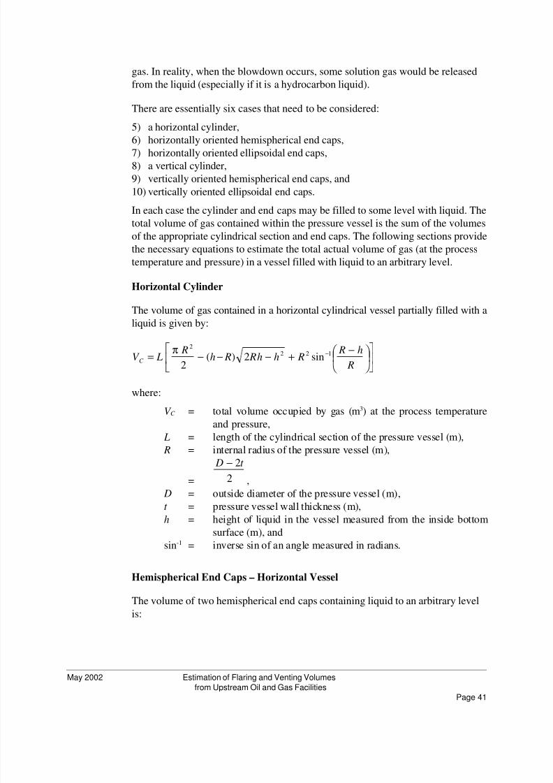
8/3/2019 Estimation of Flaring
http://slidepdf.com/reader/full/estimation-of-flaring 41/59Page 41
May 2002 Estimation of Flaring and Venting Volumes
from Upstream Oil and Gas Facilities
gas. In reality, when the blowdown occurs, some solution gas would be released
from the liquid (especially if it is a hydrocarbon liquid).
There are essentially six cases that need to be considered:
a horizontal cylinder,5)
horizontally oriented hemispherical end caps,6)horizontally oriented ellipsoidal end caps,7)
a vertical cylinder,8)
vertically oriented hemispherical end caps, and9)
vertically oriented ellipsoidal end caps.10)
In each case the cylinder and end caps may be filled to some level with liquid. The
total volume of gas contained within the pressure vessel is the sum of the volumes
of the appropriate cylindrical section and end caps. The following sections provide
the necessary equations to estimate the total actual volume of gas (at the process
temperature and pressure) in a vessel filled with liquid to an arbitrary level.
Horizontal Cylinder
The volume of gas contained in a horizontal cylindrical vessel partially filled with a
liquid is given by:
−
+−−−= −
R
h R Rhh R Rh
R LV C
1222
sin2)(2
π
where:
V C = total volume occupied by gas (m3) at the process temperatureand pressure,
L = length of the cylindrical section of the pressure vessel (m),
R = internal radius of the pressure vessel (m),
= 2
2t D −
,
D = outside diameter of the pressure vessel (m),
t = pressure vessel wall thickness (m),
h = height of liquid in the vessel measured from the inside bottom
surface (m), and
sin-1
= inverse sin of an angle measured in radians.
Hemispherical End Caps – Horizontal Vessel
The volume of two hemispherical end caps containing liquid to an arbitrary level
is:
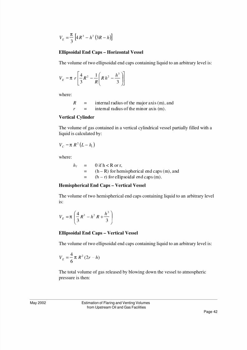
8/3/2019 Estimation of Flaring
http://slidepdf.com/reader/full/estimation-of-flaring 42/59Page 42
May 2002 Estimation of Flaring and Venting Volumes
from Upstream Oil and Gas Facilities
( )[ ]h Rh RV E
−−= 343
23π
Ellipsoidal End Caps – Horizontal Vessel
The volume of two ellipsoidal end caps containing liquid to an arbitrary level is:
−−=
3
1
3
4 322 h
h R R
Rr V E
π
where:
R = internal radius of the major axis (m), and
r = internal radius of the minor axis (m).
Vertical Cylinder
The volume of gas contained in a vertical cylindrical vessel partially filled with a
liquid is calculated by:
( )1
2 h L RV C −=π
where:
h1 = 0 if h < R or r,
= (h – R) for hemispherical end caps (m), and
= (h – r) for ellipsoidal end caps (m).
Hemispherical End Caps – Vertical Vessel
The volume of two hemispherical end caps containing liquid to an arbitrary level
is:
+−=
33
4 323 h Rh RV E π
Ellipsoidal End Caps – Vertical Vessel
The volume of two ellipsoidal end caps containing liquid to an arbitrary level is:
)2(6
4 2 hr RV E
−= π
The total volume of gas released by blowing down the vessel to atmospheric
pressure is then:
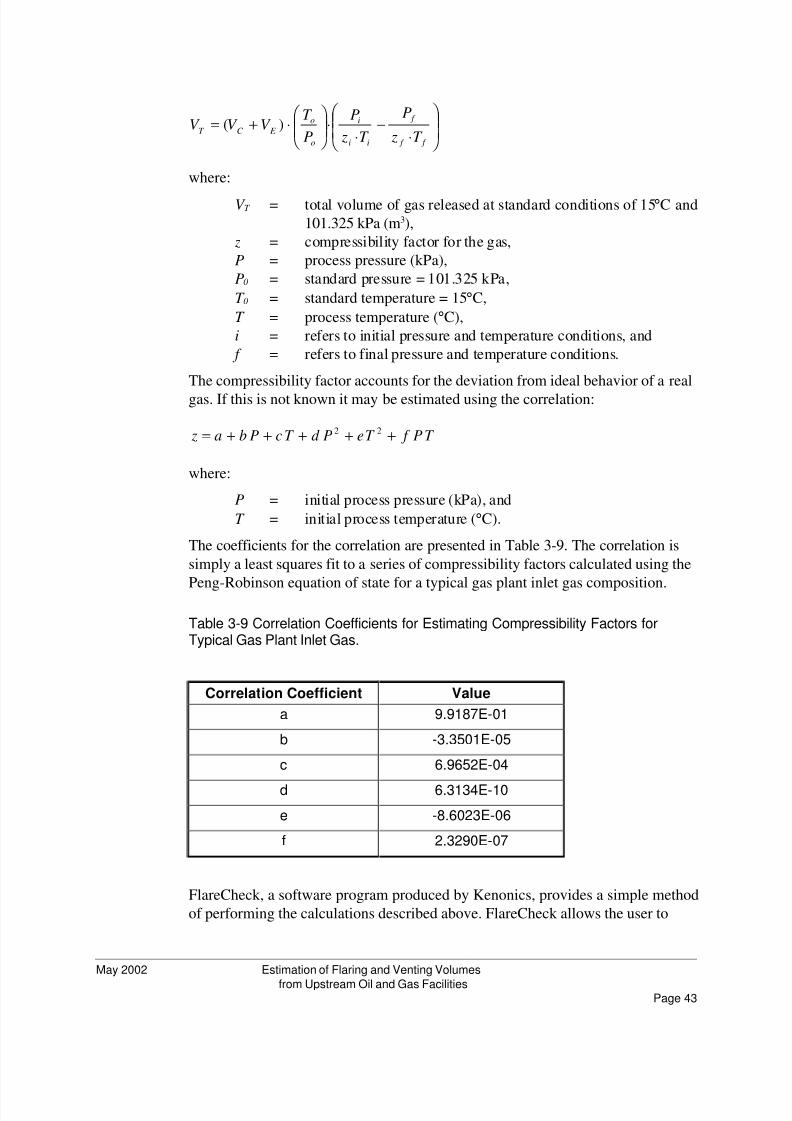
8/3/2019 Estimation of Flaring
http://slidepdf.com/reader/full/estimation-of-flaring 43/59Page 43
May 2002 Estimation of Flaring and Venting Volumes
from Upstream Oil and Gas Facilities
⋅−
⋅⋅
⋅+=
f f
f
ii
i
o
o
E C T T z
P
T z
P
P
T V V V )(
where:
V T = total volume of gas released at standard conditions of 15°C and
101.325 kPa (m3),
z = compressibility factor for the gas,
P = process pressure (kPa),
P0 = standard pressure = 101.325 kPa,
T 0 = standard temperature = 15°C,
T = process temperature (°C),
i = refers to initial pressure and temperature conditions, and
f = refers to final pressure and temperature conditions.
The compressibility factor accounts for the deviation from ideal behavior of a real
gas. If this is not known it may be estimated using the correlation:
T P f T ePd T cPba z +++++= 22
where:
P = initial process pressure (kPa), and
T = initial process temperature (°C).
The coefficients for the correlation are presented in Table 3-9. The correlation is
simply a least squares fit to a series of compressibility factors calculated using the
Peng-Robinson equation of state for a typical gas plant inlet gas composition.
Table 3-9 Correlation Coefficients for Estimating Compressibility Factors forTypical Gas Plant Inlet Gas.
Correlation Coefficient Value
a 9.9187E-01
b -3.3501E-05
c 6.9652E-04
d 6.3134E-10
e -8.6023E-06
f 2.3290E-07
FlareCheck, a software program produced by Kenonics, provides a simple method
of performing the calculations described above. FlareCheck allows the user to
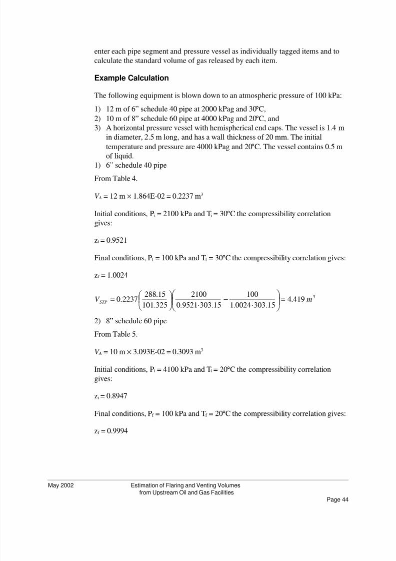
8/3/2019 Estimation of Flaring
http://slidepdf.com/reader/full/estimation-of-flaring 44/59Page 44
May 2002 Estimation of Flaring and Venting Volumes
from Upstream Oil and Gas Facilities
enter each pipe segment and pressure vessel as individually tagged items and to
calculate the standard volume of gas released by each item.
Example Calculation
The following equipment is blown down to an atmospheric pressure of 100 kPa:12 m of 6” schedule 40 pipe at 2000 kPag and 30°C,1)
10 m of 8” schedule 60 pipe at 4000 kPag and 20°C, and2)
A horizontal pressure vessel with hemispherical end caps. The vessel is 1.4 m3)
in diameter, 2.5 m long, and has a wall thickness of 20 mm. The initial
temperature and pressure are 4000 kPag and 20°C. The vessel contains 0.5 m
of liquid.
6” schedule 40 pipe1)
From Table 4.
V A = 12 m × 1.864E-02 = 0.2237 m3
Initial conditions, Pi = 2100 kPa and Ti = 30°C the compressibility correlation
gives:
zi = 0.9521
Final conditions, Pf = 100 kPa and Tf = 30°C the compressibility correlation gives:
zf = 1.0024
3419.415.3030024.1
10015.3039521.0
2100325.10115.2882237.0 mV STP =
⋅−
⋅
=
8” schedule 60 pipe2)
From Table 5.
V A = 10 m × 3.093E-02 = 0.3093 m3
Initial conditions, Pi = 4100 kPa and Ti = 20°C the compressibility correlation
gives:
zi = 0.8947
Final conditions, Pf = 100 kPa and Tf = 20°C the compressibility correlation gives:
zf = 0.9994
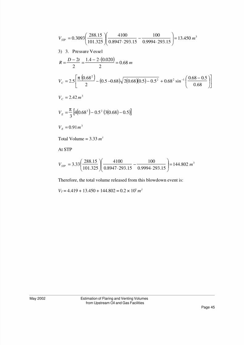
8/3/2019 Estimation of Flaring
http://slidepdf.com/reader/full/estimation-of-flaring 45/59Page 45
May 2002 Estimation of Flaring and Venting Volumes
from Upstream Oil and Gas Facilities
3450.1315.2939994.0
100
15.2938947.0
4100
325.101
15.2883093.0 mV STP =
⋅
−⋅
=
3. Pressure Vessel3)
( ) mt D R 68.02
020.024.122 =⋅−=−=
( )( ) ( )( )
−
+−−−= −
68.0
5.068.0sin68.05.05.068.0268.05.0
2
68.05.2 122
2π
C V
342.2 mV C =
( ) ( )( )[ ]5.068.035.068.043
23 −−=π
E V
391.0 mV E =
Total Volume = 3.33 m3
At STP
3802.14415.2939994.0
100
15.2938947.0
4100
325.101
15.28833.3 mV STP =
⋅
−⋅
=
Therefore, the total volume released from this blowdown event is:
V T = 4.419 + 13.450 + 144.802 = 0.2 × 10³ m3

8/3/2019 Estimation of Flaring
http://slidepdf.com/reader/full/estimation-of-flaring 46/59
GlossaryAppendix A
8/3/2019 Estimation of Flaring
http://slidepdf.com/reader/full/estimation-of-flaring 47/59Page A-47
May 2002 Estimation of Flaring and Venting Volumes
from Upstream Oil and Gas Facilities
Associated Gas
A certain quantity of natural gas often accompanies the production of oil from an
underground reservoir. This free gas is usually separated from the oil stream at a
battery and may be vented, flared or conserved. EUB production accounting rules
require that the quantity of gas be metered at the separator and reported on the
appropriate production accounting forms.
Casing Gas
Gas released from the casing of some heavy oil wells to maintain reasonable flow
potential from the well. Down-hole pressures are typically maintained at about 250
kPa by opening the vent valve on the casing. Casing gas may be vented to the
atmosphere, collected and flared or incinerated or conserved and used as fuel or
further processed.
Central Battery
A central battery is similar to a single-well battery except that it receives
production from more than one well and is usually much larger. It is generally
equipped with separation, metering, storage, loading, treatment, pumping,
compression and flaring facilities. Often, it is manned continuously during the
day.
Emulsion Treater
A process by whicg an oil-water emulsion is separated into its constituent phases
(i.e., oil and water) primarily by the addition of heat. The reduction in pressure
from the separator and the addition of heat tends to drive solution gas from the
produced oil.
Evaporation Losses
Losses of stable (i.e., not boiling or flashing) hydrocarbon product from
production storage tanks due to diurnal (i.e., daily) atmospheric temperature and
pressure changes and liquid level changes within the tank.
Flared Emissions
Waste gas that is combusted as an open flame at the exit of a flare stack. The
flame is maintained by the use of a pilot or electronic igniter. Flares have
destruction efficiencies ranging from <70 percent to >98 percent depending on
design, composition and heating value of the waste gas, exit velocities and local
wind conditions.Flashing Losses
Losses from hydrocarbon storage tanks resulting from directing a hydrocarbon
liquid stream from a vessel, where it has been in contact with hydrocarbon gas at
an elevated pressure, into an atmospheric storage tank. The solution gas absorbed
in the oil quickly flashes/boils off resulting in increased emissions from the tank.
8/3/2019 Estimation of Flaring
http://slidepdf.com/reader/full/estimation-of-flaring 48/59Page A-48
May 2002 Estimation of Flaring and Venting Volumes
from Upstream Oil and Gas Facilities
Gas Battery
The simplest type of gas production facility. It is usually equipped with separation,
metering, dehydration and compression facilities.
Gas Boot
Production facilities equipped with a vapour recovery system on the storage tanks
often have a gas boot as the final vessel prior to the storage tanks. The purpose of
the gas boot is to reduce the pressure of the hydrocarbon liquid stream to as close
to atmospheric as possible prior to entering the atmospheric tanks. Gas boots may
be operated at temperatures and pressures in the region of 25°C and 25 kPag.
Gas Gathering System
A network of pipelines designed to transport gas from the field to a gas processing
plant or to market. Gas gathering systems generally fall into one of three
categories depending on the type of equipment installed for hydrate control: lowpressure, heated or dehydrated.
Gas Processing Plant
A facility for extracting condensable hydrocarbons from natural gas, and for
upgrading the quality of the gas to market specifications (i.e., removing
contaminants such as H2O, H2S and CO2). Some compression may also be
required. Each facility may comprise a variety of treatment and extraction
processes, and for each of these there is often a range of technologies that may be
used.
Pressure-Relief ValvesPressure relief or safety valves are used to protect process piping and vessels from
being accidentally over-pressured. They are spring loaded so that they are fully
closed when the upstream pressure is below the set point, and only open when the
set point is exceeded. Relief valves open in proportion to the amount of
overpressure to provide modulated venting. Safety valves pop to a full-open
positions on activation.
When relief or safety valves reseat after having been activated, they often leak
because the original tight seat is not regained either due to damage of the seating
surface or a build-up of foreign material on the seat plug. As a result, they are
often responsible for fugitive emissions. Another problem develops if theoperating pressure is too close to the set pressure, causing the valve to "simmer"
or "pop" at the set pressure.
Gas that leaks from a pressure-relief valve may be detected at the end of the vent
pipe (or horn). Additionally, there normally is a monitoring port located on the
bottom of the horn near the valve.
Satellite Battery
8/3/2019 Estimation of Flaring
http://slidepdf.com/reader/full/estimation-of-flaring 49/59Page A-49
May 2002 Estimation of Flaring and Venting Volumes
from Upstream Oil and Gas Facilities
An intermediate production facility located between a group of wells and a central
battery. There are two separators and associated sets of metering equipment at
each satellite battery. One train is used to compile proration data on the
commingled effluent from all but one of the group of wells. The other is used to
test the remaining well. A regular test is performed on each of the wells.
Single-Well Battery
The simplest type of oil battery. It is equipped with separation, metering, storage,
loading and flaring facilities. Depending on the amount and nature of the
production, it may also comprise selected treatment, pumping and compression
facilities.
Solution Gas
Refers to gas absorbed in a liquid hydrocarbon stream at an elevated pressure.
When the pressure is reduced as a result of processing the hydrocarbons, a new
thermodynamic equilibrium is achieved and some solution gas may be desorbed
from the liquid stream.
Standard Reference Conditions
Most equipment manufacturers reference flow, concentration and equipment
performance data at ISO standard conditions of 15°C, 101.325 kPa, sea level and
0.0 percent relative humidity.
Total Hydrocarbons
All compounds containing at least one hydrogen atom and one carbon atom, with
the exception of carbonates and bicarbonates.
Total OrganicCompounds (TOC)TOC comprises all VOCs plus all non-reactive organic compounds (i.e., methane,
ethane, methylene chloride, methyl chloroform, many fluorocarbons, and certain
classes of per fluorocarbons).
Vented Emissions
Vented emissions are releases to the atmosphere by design or operational practice,
and may occur on either a continuous or intermittent basis. The most common
causes or sources of these emissions are gas operated devices that use natural gas
as the supply medium (e.g., compressor start motors, chemical injection and
odourization pumps, instrument control loops, valve actuators, and some types of
glycol circulation pumps), equipment blowdowns and purging activities, andventing of still-column off-gas by glycol dehydrators.
Volatile Organic ompounds (VOC)
Any compound of carbon, excluding carbon monoxide, and carbon dioxide,
which participates in atmospheric chemical reactions. This excludes methane,
ethane, methylene chloride, methyl chloroform, many fluorocarbons, and certain
classes of per fluorocarbons.
8/3/2019 Estimation of Flaring
http://slidepdf.com/reader/full/estimation-of-flaring 50/59Page A-50
May 2002 Estimation of Flaring and Venting Volumes
from Upstream Oil and Gas Facilities
Well
A surface facility that is used to produce oil and gas from a hydrocarbon reservoir.
It consists of the wellhead and may or may not have metering facilities and some
production equipment (e.g., pumpjack compressor, line heater, dehydrator,
storage tank, etc).

8/3/2019 Estimation of Flaring
http://slidepdf.com/reader/full/estimation-of-flaring 51/59
AcronymsAppendix B

8/3/2019 Estimation of Flaring
http://slidepdf.com/reader/full/estimation-of-flaring 52/59Page B-52
May 2002 Estimation of Flaring and Venting Volumes
from Upstream Oil and Gas Facilities
AOFP - Absolute Open Flow Potential
API - American Petroleum Institute
BTEX - Benzene, Toluene, Ethyl benzene and Xylene (mixed isomers)
CAPP - Canadian Association of Petroleum Producers
DEG - Diethylene Glycol
EC - Environment CanadaEPA - Environmental Protection Agency
EUB - Energy and Utilities Board (Alberta)
GOR - Gas-to-Oil Ratio
GRI - Gas Research Institute (now GTI)
GTI - Gas Technology International
NPS - Nominal Pipe Size
ppb - Parts Per Billion
ppm - Parts Per Million
PRV - Pressure Relief Valve
PSV - Pressure Safety Valve
STP - Standard Temperature and Pressure (i.e., 15°C and 101.325 kPa)
TEG - Triethylene Glycol
THC - Total Hydrocarbons
TOC - Total Organic Compounds
U.S. EPA - U.S. Environmental Protection Agency
VOC - Volatile Organic Compound

8/3/2019 Estimation of Flaring
http://slidepdf.com/reader/full/estimation-of-flaring 53/59
Conversion FactorsAppendix C
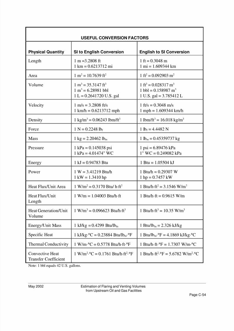
8/3/2019 Estimation of Flaring
http://slidepdf.com/reader/full/estimation-of-flaring 54/59Page C-54
May 2002 Estimation of Flaring and Venting Volumes
from Upstream Oil and Gas Facilities
USEFUL CONVERSION FACTORS
Physical Quantity SI to English Conversion English to SI Conversion
Length 1 m =3.2808 ft
1 km = 0.6213712 mi
1 ft = 0.3048 m
1 mi = 1.609344 km
Area 1 m2 = 10.7639 ft2 1 ft2 = 0.092903 m2
Volume 1 m3 = 35.3147 ft3
1 m3 = 6.28981 bbl
1 L = 0.2641720 U.S. gal
1 ft3 = 0.028317 m3
1 bbl = 0.158987 m3
1 U.S. gal = 3.785412 L
Velocity 1 m/s = 3.2808 ft/s
1 km/h = 0.6213712 mph
1 ft/s = 0.3048 m/s
1 mph = 1.609344 km/h
Density 1 kg/m3 = 0.06243 lbm/ft3 1 lbm/ft3 = 16.018 kg/m3
Force 1 N = 0.2248 lbf 1 lbf = 4.4482 N
Mass 1 kg = 2.20462 lbm 1 lbm = 0.45359737 kg
Pressure 1 kPa = 0.145038 psi
1 kPa = 4.01474" WC
1 psi = 6.89476 kPa
1" WC = 0.249082 kPa
Energy 1 kJ = 0.94783 Btu 1 Btu = 1.05504 kJ
Power 1 W = 3.41219 Btu/h1 kW = 1.3410 hp 1 Btu/h = 0.29307 W1 hp = 0.7457 kW
Heat Flux/Unit Area 1 W/m2 = 0.3170 Btu/ h·ft2 1 Btu/h·ft2 = 3.1546 W/m2
Heat Flux/Unit
Length
1 W/m = 1.04003 Btu/h·ft 1 Btu/h·ft = 0.9615 W/m
Heat Generation/Unit
Volume
1 W/m3 = 0.096623 Btu/h·ft3 1 Btu/h·ft3 = 10.35 W/m3
Energy/Unit Mass 1 kJ/kg = 0.4299 Btu/lbm 1 Btu/lbm = 2.326 kJ/kg
Specific Heat 1 kJ/kg·°C = 0.23884 Btu/lbm·°F 1 Btu/lbm·°F = 4.1869 kJ/kg·°C
Thermal Conductivity 1 W/m·°C = 0.5778 Btu/h·ft·°F 1 Btu/h·ft·°F = 1.7307 W/m·°C
Convective Heat
Transfer Coefficient1 W/m2·°C = 0.1761 Btu/h·ft2·°F 1 Btu/h·ft2·°F = 5.6782 W/m2·°C
Note: 1 bbl equals 42 U.S. gallons.

8/3/2019 Estimation of Flaring
http://slidepdf.com/reader/full/estimation-of-flaring 55/59
ReferencesAppendix D
8/3/2019 Estimation of Flaring
http://slidepdf.com/reader/full/estimation-of-flaring 56/59Page D-56
May 2002 Estimation of Flaring and Venting Volumes
from Upstream Oil and Gas Facilities
API (American Petroleum Institute). 1991. Evaporation Loss from Fixed-roof
Tanks. Washington, D.C. API Bulletin No. 2518. Second Edition. 39 pp.
API. 1997. Production Tank Emissions Model (E&P TANK Version 1.0).
Software Number 4660.
Beggs, Dale H. 1987. Petroleum Engineering Handbook. Chapter 22. Oil System
Correlations.
CAPP (Canadian Association of Petroleum Producers). 2001. A Suggested
Approach to Completing the National Pollutant Release Inventory (NPRI)
for the Upstream Oil and Gas Industry. Prep. by Clearstone Engineering.
Calgary, AB.
CAPP. 1999a. A Detailed Inventory of CH4 and VOC Emissions From Upstream
Oil and Gas Operations in Canada. Prep. by Clearstone Engineering.
Report No. 1999-0010. Calgary, AB.
CAPP. 1999b. Global Climate Change Voluntary Challenge Guide. Prep. by Altus
Environmental Engineering Ltd. Report No.1999-0007. Calgary, AB.
CAPP (Canadian Association of Petroleum Producers). 1992. A Detailed
Inventory of CH4 and VOC Emissions From Upstream Oil and Gas
Operations in Alberta: Volume 3 – Results of the Field Validation
Program. Prep. by Clearstone Engineering. Calgary, AB.
DB Robinson Research Ltd. 1997. E&P TANK Version 1.0. A Program for
Estimating Emissions from Hydrocarbon Production Tanks. Availablefrom American Petroleum Institute (API).
Erno, B. and R. Schmitz. 1996. Measurements of Soil Gas Migration Around Oil
and Gas Wells in the Lloydminster Area. The Journal of Canadian
Petroleum Technology. Volume 35. No. 7.
EUB. Undated. Correcting Produced Gas Volumes to Include Unmetered Solution
Gas. Calgary, AB.
EUB. 2001. Upstream Petroleum Industry Flaring Report. For the Year Ending
December 31, 2000. ST2001-60B. July 2001. Calgary, AB.
EUB. 1999. Guide 60. Upstream Petroleum Industry Flaring Requirements. July
1999. Calgary, AB.
EUB. 1999. Guide 40. Pressure and Deliverability Testing Oil and Gas Wells –
Minimum Requirements and Recommended Practices. Calgary, AB.

8/3/2019 Estimation of Flaring
http://slidepdf.com/reader/full/estimation-of-flaring 57/59Page D-57
May 2002 Estimation of Flaring and Venting Volumes
from Upstream Oil and Gas Facilities
EUB. 1997. Surface Casing Vent Blow File. Database. Calgary, AB.
EUB. 1994. ID 94-01 – Measurement of Oil, Gas and Water Production. January
1994. Calgary, AB.
EUB. 1991. IL 91-09 – Exemption From Gas Measurement Crude Oil / BitumenWells. July 1991. Calgary, AB.
EUB. 1991. ID 91-03 – Heavy Oil / Oil Sands Operations. March 1991. Calgary,
AB.
Meyers, Duane. 1996. Methane Emissions from the Natural Gas Industry. Volume
14: Glycol Dehydrators. Prep. By Radian International LLC. For GRI and
EPA. Report No. EPA-600/R-96-080n. Research Triangle Park. NC.
Picard, D.J., and S.K. Sarkar. 1993. A Technical and Cost Evaluation of Options
for Reducing Methane and VOC Emissions from Upstream Oil and GasOperations. A report prepared by Clearstone Engineering Ltd. and Fluor
Daniel Canada, Inc. for Canadian Association of Petroleum Producers.
Calgary, Alberta.
Schmitz, R.A., T.E. Cook, G.M.J. Ericson, M.M. Klebek, R.S. Robinson, and D.R.
Van Stempvoort. 1996. A Risk Based Management Approach to the
Problem of Gas Migration. Presented at the Society of Petroleum
Engineers International Conference on Health, Safety & Environment.
New Orleans, LA. June 9-12 1996.
Shapiro, Ascher H. 1953. The Dynamics and Thermodynamics of CompressibleFluid Flow. John Wiley & Sons. Toronto.
Thompson, P.A., A.P. Espenscheid, C.A. Berry, and D.B. Myers. 1994. Technical
Reference Manual for GRI-GLYCalc: A Program for Estimating Emissions
From Glycol Dehydration of Natural Gas. Version 2.0. Prep. by Radian
Corporation for Gas Research Institute. Chicago, IL. 101 pp.
Ullman, P.M., M.J. Zelensky, W.A. Murray, and D.S. Chadder. 1987. Air Quality
Impact Assessment: Phase 4 Air Quality Study - Lindbergh Oil Sands
Sector. Prep. by Environmental Management Associates for Lindbergh
Environmental Study Group. Calgary, Alberta.

8/3/2019 Estimation of Flaring
http://slidepdf.com/reader/full/estimation-of-flaring 58/59
BibliographyAppendix E

8/3/2019 Estimation of Flaring
http://slidepdf.com/reader/full/estimation-of-flaring 59/59
CAPP. 2000. A Suggested Approach to Completing the National Pollutant Release
Inventory (NPRI) for the Upstream Oil and Gas Industry. Prep. by
Clearstone Engineering Ltd. Calgary, AB.
DB Robinson Research Ltd. 1997. E&P TANK Version 1.0. A Program for
Estimating Emissions from Hydrocarbon Production Tanks. Availablefrom American Petroleum Institute (API).
Gas Technology Canada (now GTI Canada). 1998. Handbook for Estimating
Methane Emissions from Canadian Natural Gas Systems. Prep. by
Clearstone Engineering Ltd., Enerco Engineering Ltd. and Radian
International. Guelph, ON.
GRI GlyCalc. 1994. A program for estimating emissions from the reboiler still
column of glycol dehydration units. Available from GRI.
Kenonic Controls. 1999. FlareCheck. A program for estimating vessel,compressor, pipeline, and well blowdowns, venting from storage tanks,
and gas released through pressure relief valves and regulating valves.
Available from Kenonic Controls (www.kenonic.com).
U.S. EPA Tanks 4.0. 1999. A program for estimating normal evaporation losses
(i.e., standing and breathing losses) from production storage tanks.
Available from U.S. EPA (www.epa.gov/ttn/chief ).