DOCUMENT

Spectral Line Catalogue from Herschel-HIFISpectral Scans:

Explanatory Supplement

Prepared by David Teyssier (ESAC), Lisa Benamati (IRAP)Reference HERSCHEL-HSC-DOC-2196Issue 1Revision Release 1.0Date of Issue 2017-12-21Status For releaseDocument Type Release NoteDistribution HSC

ESA UNCLASSIFIED - Releasable to the public

ESA UNCLASSIFIED - Releasable to the public HERSCHEL-HSC-DOC-2196

Document approval

Prepared by: D. Teyssier, L. Benamati Date: 2017-12-21

Approved by: Date:

Change log

Version Date Change Author0.1 2017-06-16 First draft of document David Teyssier, Lisa Benamati1.0 2017-12-21 Final document issue David Teyssier, Lisa Benamati

2

ESA UNCLASSIFIED - Releasable to the public HERSCHEL-HSC-DOC-2196

1 IntroductionThe Heterodyne Instrument for the Far-Infrared (HIFI, (7)) was the high-resolution spectrometeron-board Herschel, offering a continuous spectral coverage in the ranges [480–1270] and [1430–1910] GHz with a resolving power in excess of 107. One of the richest output of the HIFIscientific database lies in the hundreds of spectral line surveys it conducted using its SpectralScan observing mode. Overall, HIFI collected around 500 observations in this mode, over abouta hundred of different lines-of-sight, in partial or full spectral coverage.

A dedicated effort was conducted in order to extract and identify as many spectral lines as pos-sible from these observations, using baseline-corrected versions of the Spectral Scan productsspecially curated as Highly-Processed Data Products (HPDP, (17)). The approach is based onan automatic spectral feature detection algorithm, coupled to a spectroscopy data-base used toassign the most likely species and transition to any detection. The process used a combinationof tools specially coded in HIPE1, and functionalities offered in CASSIS2.

This document describes the method used to generate and validate the Spectral Line Catalogueobtained from these observations. The Catalogue is made available through the Herschel ScienceArchive as a Highly-Processed Data Product, and we provide here further information about thecontent of this data-set.

2 Cautionary notesThe primary goal of this work is to provide a list of spectral features present in the HIFI spectralscans, and offer a best-guess of which line and transition that each correspond to. The complete-ness of the catalogue is limited by the data noise (as is explained in the following section, a SNRthreshold of 5 was applied to the selection of spectral line feature), as well as the complexity ofthe line profiles (intrinsic to the source, or altered by possible OFF position contamination). Ontop of that, not all spectral lines could be assigned to a specific transition (so-called U-lines), andsome could actually correspond to multiple solutions (so-called blended lines). The U-lines arenot provided as output of this study (see also Sect. 8).

Although all integrity checks show a high level of reliability in both line detection and transitionassignment (see Sect. 7), special care should be taken when using lines with low intensity (typ-ically below some hundreds of mK) and/or signal-to-noise ratio, in particular when those linesare stamped as blends. Finally, the fitted line intensities should be used with precaution whenthe line profiles deviate from a simple Gaussian, or when the spectral line density is particularlyhigh (which will manifest also in the line blends) – see also Sect. 5.2 for additional warning flagsprovided with the catalogue.

1https://www.cosmos.esa.int/web/herschel/hipe-download2http://cassis.irap.omp.eu

3

ESA UNCLASSIFIED - Releasable to the public HERSCHEL-HSC-DOC-2196

3 The HIFI Spectral Scans

3.1 Archive content and science readinessWe consider here the ∼500 Spectral Scan observations obtained in standard observing mode (incontrast with those performed in the so-called engineering mode) with one of the three possiblereferencing schemes for this mode (namely Double Beam Switching, Load Chop and FrequencySwitching). Of those, we ignored the 18 Spectral Scan observations stamped as non-public, asthey usually made use of non-standard observing modes or instrument configuration settings.The standard product generation pipeline provides calibrated deconvolved spectra in each polar-isation for each observation, and takes care of masking all spurious spectral features still presentin the Level 2 products (see e.g. the HIFI Product Explained document, or the Spectral Scancookbook). What the automatic pipeline does not cover, though, is the treatment of any residualbaseline distortion resulting from an imperfect bandpass calibration (e.g. standing waves, seeSection 5.3 of the HIFI Handbook for further details).

3.2 Baseline-corrected Spectral Scans and considered sampleIn order to circumvent those residual artefacts, baseline-corrected spectra have been generatedby the Herschel Science Centre (HSC) in the form of Highly Processed Data Products3 (17).Due to the semi-automatic approach used in this process, there are some limitations to the typeof observations that can be accurately treated by this method. In particular, its result is relativelypoor in case of relatively line-rich spectra, or complex, broad, line profiles. This is particularlytrue for observations towards sources such as Orion KL (e.g. (5)), the SgB2 lines-of-sight (e.g.(4), (18)), η Carina (e.g.(10)) or line rich evolved stars like IRC+10216 (e.g. (3)), VY CMa(e.g. (1)) or OH231.8+4.2 (e.g. (2)). When applied to these complicated sources, the baselinecorrection usually results in erroneous line intensities and/or profiles, which we decided wouldnot qualify as HPDP.

As a consequence, about 1/3 of all observed Spectral Scans was discarded from this exercise,and it was therefore decided that the same crtierion should apply to the sample eventually usedto generate the Spectral Line Catalogue described in this document. Table 7 gives an inventory ofthe omitted observations, together with references to past or future work expected to provide theinformation missing from the baseline-corrected data-set provided by the HSC. The expectationis that those products (both baseline corrected and Spectral Line Catalogue) should eventuallybecome available as User-Provided Data Products4.

Exceptionally, however, Spectral Line Catalogues were generated for sources where the baselinecorrection was not considered accurate enough to release the corrected data themselves, butwhere, however, the line detection and species identification would make sense. For those, noinformation about line intensity or line width is provided. They are listed in Table 8. Thisapproach is also followed for some particular cases of the catalogue generation where input datahave been smoothed for dedicated purpose (see Section 4.2.2).

3http://archives.esac.esa.int/hsa/legacy/HPDP/HIFI/HIFI_spectral_scans/4https://www.cosmos.esa.int/web/herschel/user-provided-data-products

4

ESA UNCLASSIFIED - Releasable to the public HERSCHEL-HSC-DOC-2196

Figure 1: Illustration of a baseline-corrected HPDP for obsid 1342192328. The upper panelshows the products from the standard pipeline generation (black) with the removed baseline inred. The middle panel (blue spectra) shows the resulting baseline-corrected spectra. Finally,the lower panel shows the removed baseline. Note that the removed baseline contains both theintrinsic source continuum and the residual baseline artefacts.

5

ESA UNCLASSIFIED - Releasable to the public HERSCHEL-HSC-DOC-2196

In total, the catalogue generation considered an input of 339 baseline-corrected spectral scans.Table 6 summarises the sources they correspond to, and the spectral coverages offered by theassociated observations.

4 Generation of the Spectral Line Catalogue

4.1 MethodThe input to the catalogue generation is in fact based on the merging of the two polarisationspectra provided for each of the baseline-corrected Spectral Scans. In all but two cases (obsid1342181163, where the H spectrum is plagued with artefacts that we could not clean effectively,and obsid 1342253144 where only the V channel was selected by the observer), both H and Vpolarisations are averaged. Note that there are known reasons for the H and V spectra to displayslightly discrepant information, both on line and continuum (see e.g. Section 5.8.4 of the HIFIhandbook).

Based on these input files, the catalogue generation essentially relies on a dedicated task de-veloped within HIPE and called identifyLines – a general description of the task and itsparameters is given in the correspond HIPE manual page5. The task works in two steps:

◦ First, the spectral feature detection is performed, based on an automatic line masking func-tionality provided in the HIPE software (so-called smoothBaseline, see the task descriptionin HIPE manual6). The main parameters for this stage of the processing are (i) the numberof segments to split the input spectrum into in order to speed up the process, (ii) the spec-tral smoothing factor, usually used to lower the noise rms, (iii) the best-guess line widthfor emission and absorption lines respectively, (iv) the signal-to-noise (SNR) threshold fora feature to qualify as a robust detection. Detected lines are then fit with a Gaussian lineprofile and the outcome is stored in the table. For absorption lines, the resulting line willappear with negative intensity because the input spectrum has had its baseline subtracted(Section 3.2).

◦ The second step consists of assigning the most likely species and transition to each of thedetections resulting from the first step. For this a line list template is used. Section 4.3describes how this template was built. Because this line list template provides line fre-quencies in the Local Standard of Rest (LSR), a fundamental step in the assignment is theassessment of the systemic velocity of the studied target in the LSR, called thereafter vLSR.We explain in Section 4.3.2 how this latter was figured out for each observation.

4.2 Line detectionThe HIPE task identifyLines was used systematically on all 339 baseline-correctedpolarisation-averaged spectra described in Section 3.2. We used the following parameters as

5http://herschel.esac.esa.int/hcss-doc-15.0/load/hifi_um/html/hdrg_lineid.html6http://herschel.esac.esa.int/hcss-doc-15.0/load/hcss_urm/html/herschel.ia.toolbox.

spectrum.standingwaves.SmoothBaselineTask.html

6

ESA UNCLASSIFIED - Releasable to the public HERSCHEL-HSC-DOC-2196

default:

◦ nbOfSplit = 4 (i.e. split the spectrum in four equal ranges to speed up the process)

◦ smoothBox = 7 (i.e. smooth the spectra with a 7 channel box to lower the rms and increasethe line detectability)

◦ fwhmAbsorption = 1 km/s (best-guess line width for absorption lines – note that this num-ber had to be increased for some obsids exhibiting broader absorption lines).

◦ fwhmEmission = 4 km/s (best-guess line width for emission lines – note that this numberhad to be increased for some obsids exhibiting broader emission lines).

◦ snrType = ”Intensity” (parameter used to compute the signal to noise ratio – the alternativeis Flux)

◦ minSNR = 5 (value of the minimum signal to noise ratio – all lines detected with a valuesmaller than that are rejected)

The decision on the SNR threshold is based on an exploratory study of the outcome of the lineidentification for various values of the SNR. The threshold of 5 was found to be a good trade-off

between limiting to the maximum the number of false positives (which would show up at toolow SNR) while still allowing recognition of lines appearing as an unequivocal detection. Therewere, however, still some false positive resulting from the chosen threshold, and a dedicatedcleaning exercise was then performed as a subsequent step.

4.2.1 Line parameters

Each detected spectral feature is then fitted by a model consisting of a Gaussian sitting on topof a first order polynomial continuum. The fitted parameters and their uncertainties are thentabulated in the line identification table (see Section 5.1). It should be noted that Gaussian fitsare performed irrespective of the exact line profile, and as such there is no additional informationabout the existence of e.g. outflows or peculiar line profiles (e.g. top hat in AGB stars). Thisalso means that the derived line parameters (width, centroid, integrated intensities) might not befully representative of the values applying to the more complex line profiles.

4.2.2 Smoothed and un-smoothed input data

Because the initial spectral feature detection step relies on an automatic line mask generation,there can be particular cases where the line profile of a given feature makes it difficult for thealgorithm to yield a detection. This will generally happen with relatively broad lines, lines inabsorption, or complex profile such as P-Cygni ones, or their look-alike that arise in case ofsevere OFF position contamination (see also (16)). In these cases, the task was shown to do abetter job when the input spectra was smoothed in frequency.

The positive consequence of this alternative process is that not only complex profiles would endup being detected and then fed to the line identification step, but also weaker lines initially buriedinto the noise at native resolution would be picked up by the detection step, and also make it intothe catalogue table. On the downside, however, the smoothing needed to achieve such result issometimes relatively large compared to the intrinsic line widths and, as a consequence, the fitted

7

ESA UNCLASSIFIED - Releasable to the public HERSCHEL-HSC-DOC-2196

line parameters of the severely broadened line profiles would no longer be representative of thereal line characteristics. Also, for very crowded spectra, significant smoothing will blend lineslocated close to each other, potentially precluding to detect them as they would no longer bespectrally resolved.

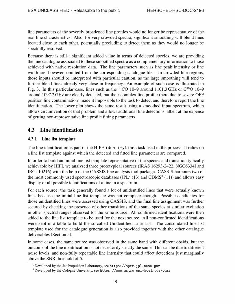
Because there is still a significant added value in terms of detected species, we are providingthe line catalogue associated to these smoothed spectra as a complementary information to thoseachieved with native resolution data. The line parameters such as line peak intensity or linewidth are, however, omitted from the corresponding catalogue files. In crowded line regions,those inputs should be interpreted with particular caution, as the large smoothing will tend tofurther blend lines already very close in frequency. An example of such case is illustrated inFig. 3. In this particular case, lines such as the 13CO 10–9 around 1101.3 GHz or C18O 10–9around 1097.2 GHz are clearly detected, but their complex line profile (here due to severe OFFposition line contamination) made it impossible to the task to detect and therefore report the lineidentification. The lower plot shows the same result using a smoothed input spectrum, whichallows circumvention of that problem and allows additional line detections, albeit at the expenseof getting non-representative line profile fitting parameters.

4.3 Line identification4.3.1 Line list template

The line identification is part of the HIPE identifyLines task used in the process. It relies ona line list template against which the detected and fitted line parameters are compared.

In order to build an initial line list template representative of the species and transition typicallyachievable by HIFI, we analysed three prototypical sources (IRAS 16293-2422, NGC6334I andIRC+10216) with the help of the CASSIS line analysis tool package. CASSIS harbours two ofthe most commonly used spectroscopic databases (JPL7 (13) and CDMS8 (11)) and allows easydisplay of all possible identifications of a line in a spectrum.

For each source, the task generally found a lot of unidentified lines that were actually knownlines because the initial line list template was not complete enough. Possible candidates forthose unidentified lines were assessed using CASSIS, and the final line assignment was furthersecured by checking the presence of other transitions of the same species at similar excitationin other spectral ranges observed for the same source. All confirmed identifications were thenadded to the line list template to be used for the next source. All non-confirmed identificationswere kept in a table to build the so-called Unidentified Line List. The consolidated line listtemplate used for the catalogue generation is also provided together with the other cataloguedeliverables (Section 5).

In some cases, the same source was observed in the same band with different obsids, but theoutcome of the line identification is not necessarily strictly the same. This can be due to differentnoise levels, and non-fully repeatable line intensity that could affect detections just marginallyabove the SNR threshold of 5.

7Developed by the Jet Propulsion Laboratory, see https://spec.jpl.nasa.gov8Developed by the Cologne University, see https://www.astro.uni-koeln.de/cdms

8

ESA UNCLASSIFIED - Releasable to the public HERSCHEL-HSC-DOC-2196

4.3.2 Source velocity

The HIFI pipeline provided spectral with a frequency scale calibrated in the LSR. As such, alllines appear shifted by the source systemic velocities with respect to the LSR. This velocityhence needs to be provided to the line identification task in order to related directly the fitted linecentroid to that of the LSR line frequencies tabulated in the spectroscopic database, and thereforein the line list template.

In order to determine the best guess value of the source systemic velocity, we relied primarily onthe detection of the 12CO (5-4) line (or the 13CO (5-4) line if the profile of the 12CO line was toocomplex) in band 1a. When those were not observed or non-detected, our first backup was to tryand recognise the H12CO+ (7-6) or H12CN (7-6) lines present in band 1b. When even this wasnot possible, we then tried to rely on higher transitions of the same molecules which could havebeen detected in other bands. When none of this was available, we finally relied on velocitiesreported in the literature. This initial centroid value is tabulated as v0 in Table 9.

Once the line catalogues were generated for each observation, we computed for each source themean vLSR value and its uncertainty as the respective median and the standard deviation of all vLSR

derived from an identified line in this source. The presence of high values of the vLSR uncertaintyfor some sources is due to their complex nature and structure. Indeed, some sources are knownto harbour maser lines emission, outflows, or broad emission lines. Table 9 summarises all thesenumbers, together with other statistical figures applying to the sources covered by the catalogue(e.g. line width). When only one line was identified, the vLSR is given without any uncertainty.

4.3.3 Blended Entries

When several entries from the line list template match the fitted position of a given spectralfeature, multiple entries are populated into the catalogue table. Those entries will share all of theline fitting parameters and the only difference will be in the species/transition names, as well asthe rest frequency. Those multiple entries should be interpreted as alternative line identificationand the final decision on which of those it is most likely is left to the user.

4.3.4 Unidentified Lines

It is sometimes the case that a spectral feature considered as a genuine detection does not resultin any line identification, most likely due to the incompleteness of the template line list. Suchfeatures are then considered Unidentified Lines, or U-lines. The tables of U-lines are also oneof the outputs of the whole process, however, they are not delivered in the present data-set. Thisis essentially due to a lack of resources in order to perform a dedicated validation of the corre-sponding entries, in particular to discard any false positive left-over. Those may be consideredin a subsequent release of the Spectral Line Catalogue (Section 8).

9

ESA UNCLASSIFIED - Releasable to the public HERSCHEL-HSC-DOC-2196

5 Spectral Line Catalogue ContentThe delivered Spectral Line Catalogue corresponds to the successful line detection and line iden-tification achieved on a total of 278 observations. As explained in Section 4.2.2, however, someline identifications could only be performed once the data were spectrally smoothed. As such,the full catalogue will contain multiple inputs for a given observation, with the following break-down:

◦ There are 270 observations that lead to a Spectral Line Catalogue of at least one entry whenusing the native resolution Spectral Scan data. In those, 13 observations correspond toSpectral Scan data where only sub-optimal baseline correction could be achieved (Table 8,see also Section 3.2).

◦ There are 76 observations for which complementary catalogues are provided based onsmoothed Spectral Scan data. Only 8 of those observations have no counterpart in the listof the 270 observations above, because they lead to at least one line detection only whenthe input data were smoothed.

The above material is provided in the form of tables of the detected and identified lines, to-gether with postcards aimed at illustrating the content of the tables. For each observation ID, thefollowing files are provided:

◦ at most two line lists are provided in the form of FITS files: one resulting from the spec-trum at native resolution, and, when applicable, one resulting from the spectrum smoothedto a certain resolution (see Section 4.2.2). In the latter case, no information is providedabout the line flux and width, as well as the fitted continuum level. The naming conven-tion used for those tables is <obsid> HIFI LineCatalogue <method>.fits.gz, whereobsid is the observation ID and method is either “native” or “smoothed” depending onthe spectral resolution used. Note that no particular naming convention is used to dis-criminate the 13 observations listed in Table 8. However, as for the smoothed spectracatalogues, no information is provided about the line flux, width and continuum level dueto the sub-optimal baseline correction used for those data.

◦ one, so-called prime postcard, is provided for both native and smoothed res-olution catalogues where applicable. On top of this, for crowded and/orlarge spectral coverage observations, zoomed postcards are provided innarrower chunks of spectral range. The respective file names for thoseare <obsid> HIFI LineCatalogue postcard PRIME <method>.png and<obsid> HIFI LineCatalogue postcard ZOOM <nb> <method>.png where nb

is just a running number for the various zoomed postcards generated for a given obsid.

◦ the line list template used by the identifyLines task to assign transitions to detection,and described in Section 4.3.1 is also made available9. Note that this list differs from thetwo default lists provided in the HIPE software distribution10.

9http://archives.esac.esa.int/hsa/legacy/HPDP/HIFI/HIFI_line_catalogue/

LineListTemplate.txt10http://herschel.esac.esa.int/hcss-doc-15.0/load/hifi_um/html/Hifi.Um.Sec.

LinesCatalog.html

10

ESA UNCLASSIFIED - Releasable to the public HERSCHEL-HSC-DOC-2196

◦ finally, the full catalogues for the respective native and smoothed resolutions areprovided as a concatenation of all entries from all considered obsids. Those fullcatalogues are named HIFI Spectral Line Catalogue Native Full.fits.gz andHIFI Spectral Line Catalogue Smoothed Full.fits.gz.

Although the above files will be provided by the Herschel Science Archive11, they can alsobe fetched from a dedicated legacy repository: http://archives.esac.esa.int/hsa/legacy/HPDP/HIFI/HIFI_spectral_line_catalogue/. In this repository, the above fileswill be organised in separate folders TablesNative, TablesSmoothed, PostcardsNative,PostcardsSmoothed and FullCatalogues. Within each postcard directories, sub-directoriesseparate the PRIME ones from those dedicated to zoomed ranges. On top of that, bundles of allfiles applying to one given obsid can be retrieved in the directory CataloguesPerObsid underthe names <obsid> HIFI LineCatalogue.tar.gz. The total size of the HPDP is 56 Mb.

5.1 Description of the Table DatasetsThe catalogues come in the form of table data-sets saved as FITS files. Their header contentis described in Table 1. Apart from some general meta-data about the observation itself, theheader also features some specific flags providing information of interest to the user. Those aredescribed in the next section. The table content in itself consists of one row per identified spectralfeature, and provides a mixture of information on the detected species and transition, as well ason the line characteristics. The latter are based on a Gaussian fit of the detected spectral feature.Table 2 gives the details about the columns present in the data-set.

Header Parameter Descriptionobsid Observation IDsourceId Name of the sourcelongitude Right Ascension of the source in degreeslatitude Declination of the source in degreescoordinateSystem Name of reference frame for ephemeris datasmoothingWidth Size of smoothing box (in channels) when applicablemanualMaskMin n Lower limit of manual line mask #n (optional)manualMaskMax n Upper limit of manual line mask #n (optional)localStandardOfRest Local standard of resttype Herschel product typecreator Name of the S/W that produced the productcreationDate Creation date of this productdescription Product description (here ’Herschel Spectral Line List Product’)instrument Instrument attached to this productmodelName Model name attached to this productstartDate Start date of this productendDate End date of this productformatVersion Version of product formatauthor Author of the product

11http://archives.esac.esa.int/hsa/whsa/

11

ESA UNCLASSIFIED - Releasable to the public HERSCHEL-HSC-DOC-2196

profile Line extraction methodfluxUnit Unit of the fluxesbackgroundType Type of background determinationreferences References, e.g. Herschel observations/productsexplanatoryTest Additional commentsctype1 Wavelength typecunit1 Unit of wavelength axisfwhmEmission Full Width at Half Maximum used to fit emission lines (km/s)fwhmAbsorption Full Width at Half Maximum used to fit absorption lines (km/s)

Table 1: List of Line Catalogue FITS header parameters.

Column Name Descriptionobsid Observation IDname Source Name (as given by proposer)ra Right Ascension (Eq. 2000.0) of the targetdec Declination (Eq. 2000.0) of the targetobservingMode HIFI Observing mode name (here ’HifiSScan’)spectrograph Name of spectrometer backend. Save for a handful of exceptions,

it will always be ”WBS-HV” as both polarisations should have beenaveraged to form the input spectrum

spectralResolution Spectral resolution of input spectrum (MHz). For the default LineCatalogue, this corresponds to the native resolution (around 1 MHz),while for smoothed tables, it indicates the resulting spectral bin sizeafter smoothing

database Data-base from which the line spectroscopy parameters are taken (JPLor CDMS)

species Name of the molecular or atomic speciestransition Name of the transitionrestFrequency Frequency of the line transition in the LSR (GHz)eup Upper energy level Eup of the line (K)aij Einstein coefficient Ai,j (1/s)position Fitted position of the line centroid (GHz)stdPosition Standard deviation error on the above fitted position (GHz)sideBand Name of the sideband frequency scale (here ”SSB”, i.e. Single Side-

band)v0 Position of the velocity centroid (km/s)stdV0 Standard deviation error on the fitted centroid (km/s)width† Line width of the Gaussian line fit (km/s).stdWidth† Standard deviation error on the fitted line width (km/s).flux† Integrated intensity of the fitted line (K.km/s). Note that this num-

ber is negative in case of absorption lines because the spectra used toperform the fit have been baseline-subtracted.

stdFlux† Standard deviation error on the integrated intensity (K.km/s).

12

ESA UNCLASSIFIED - Releasable to the public HERSCHEL-HSC-DOC-2196

background† Continuum level estimated within the frequency interval used for thefit (K). Because the input spectra have had their baseline subtracted,this level is essentially zero.

stdBackground† Standard deviation error on the above continuum level (K).rms RMS noise level of the spectra estimated from the spectrum on two

windows of 50 MHz on either side of the line profile (K)signalToNoiseRatio Fitted line peak signal-to-noise ratioevidence Provides a quality measure of the Gaussian fit (based on a Bayesian

statistics fitter)peakPosition Frequency position of the fitted line peak (GHz)lowerFrequencyFitWindow Lower frequency of the interval used to perform the Gaussian fit

(GHz)upperFrequencyFitWindow Higher frequency of the interval used to perform the Gaussian fit

(GHz)

Table 2: Description of the Line Catalogue table columns. †Parameter not provided in the case ofsmoothed tables (Section 4.2.2) or set to zero for obsids listed in Table 8 (see also Section 3.2).

5.2 FlagsA collection of flags have been used in order to pass on additional information to the users of theSpectral Line Catalogue. They are most often warnings about peculiarities either in the baseline-corrected data used as input, or in the table content. Table 3 lists all possible flags in the data-set,and their meaning.

Flag name DescriptionresolutionFlag Set to either ”native” or ”smoothed”, it indicates whether the catalogue was

generated with the native spectral resolution data, or with smoothed inputdata. When smoothing was applied, the value of the smoothing width isgiven given in the header as smoothingWidth

highLineDensityFlag Warns against spectra were the average line density is above 1 line/GHz.This can be indicative of less accurate line fit parameters due to sub-optimalbaseline correction

baselineCorrectionFlag Warns against possible sub-optimal baseline correction that could lead toless accurate line fit parameters

absLineFlag Indicates that absorption lines are reported in catalogue. Line fit parametersfor those should be treated with care as the automatic line masking on suchlines can sometimes be sub-optimal

manualBaselineMasking When set to true is indicates that additional line masks where added by theinstrument experts in order to generate the baseline-corrected input data. Inthose cases, the masks are given in the header. Otherwise set to false (fullyautomated baseline correction)

blendedFlag Indicates if the catalogue contains blended lines

13

ESA UNCLASSIFIED - Releasable to the public HERSCHEL-HSC-DOC-2196

v0Flag This flag will provide warning and information about table entries for whichthe fitted line centroid deviate noticeably from the mean centroid computedover the whole table. When such entries were not removed from the table,it is most likely because the line identification is considered reliable, but theline centroid fit got altered for a particular reason. The flag provides furtherhints as to why it could have been the case.

fswFlag Indicates that the input data were obtained in Frequency Switching mode.Such spectra may suffer from residual spectral ghosts

freqGroupingFlag Indicates that the input data were obtained with the frequency groupingoption. Such spectra may suffer from residual baseline artefacts, potentiallyaffecting the line detection

brightLineFlag Indicates that spectral ghosts due to bright lines are present in the standardpipeline products, and that dedicated bright line flags were involved in thegeneration of the baseline-corrected spectra used to build the catalogue

offContaminationFlag Indicate that some lines are affected by OFF position contamination. Thiswill lead to either missed line detection, or inaccurate line flux computationfrom the line fitting

Table 3: List of possible flags added in the FITS file headers.

14

ESA UNCLASSIFIED - Releasable to the public HERSCHEL-HSC-DOC-2196

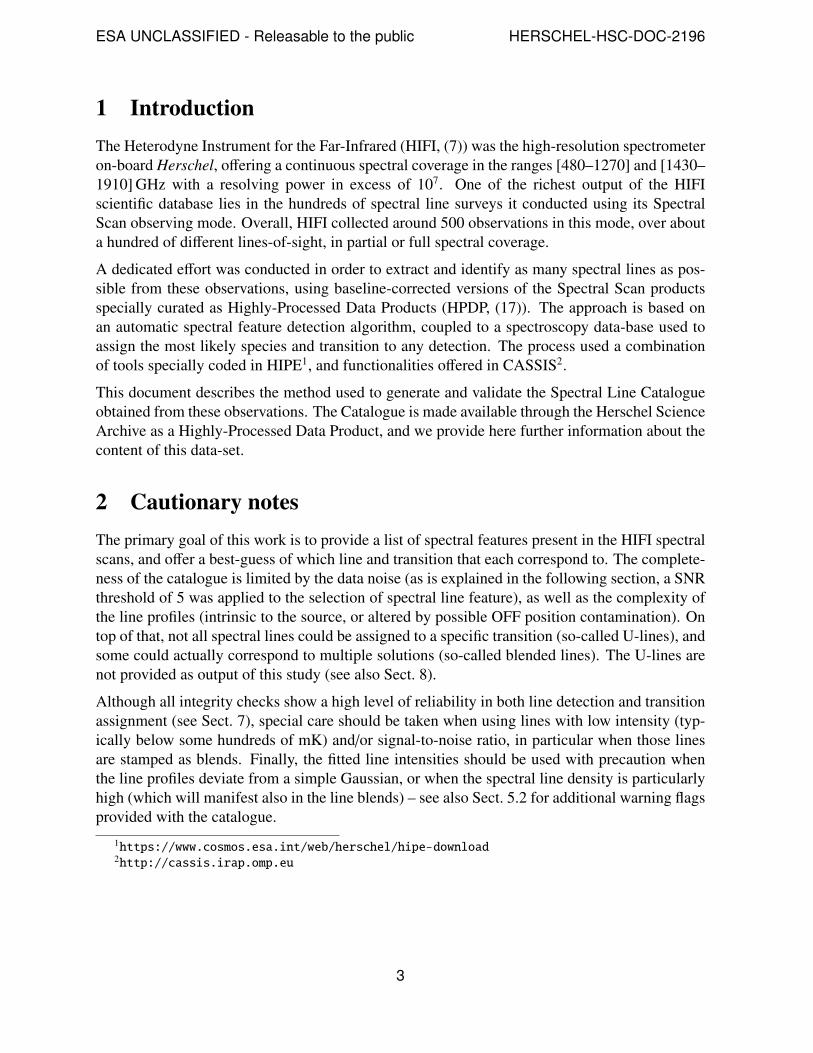
Figure 2: Illustration of a postcard for the Line Catalogue tables associated with obsid1342192328. In this particular case, both a catalogue originating from native and smoothedresolution spectra have been generated, and respective postcards are being produced. As inmost cases, there are slightly more line being detected/identified in catalogue formed from thesmoothed data.

15

ESA UNCLASSIFIED - Releasable to the public HERSCHEL-HSC-DOC-2196

Figure 3: Illustration of a postcard for the Line Catalogue tables associated with obsid1342206120 (Orion-South), where complex line profiles preclude the detection of certain (highSNR) species at native resolution (up), while they are picked up in the smoothed data. See textfor further details.

16

ESA UNCLASSIFIED - Releasable to the public HERSCHEL-HSC-DOC-2196

6 Line Catalogue StatisticsWe provide here some top-level statistics and associated plots about the content of the HIFISpectral Line Catalogue. The numbers below correspond to the native resolution catalogue. Thenumbers for the smoothed catalogue are smaller, simply because fewer observations have beenconsidered in this sub-sample.

◦ the catalogue contemplates 74 individual sources

◦ when combining those, a total of 101 unique species have been identified

◦ the combined catalogue contains 7594 entries in total, spanning 3065 unique transitions.

◦ there are, however, 1751 entries corresponding to blended identification, i.e. entries thatshare the same fitted parameters as another entry in the same source.

Figure 4 illustrates the distribution of detection per species for both the native and smoothedresolution catalogues. This simply indicates the number of occurrence of a given species de-tection, when accumulating all the relevant transitions. Note surprisingly, the most frequentlyreported molecules (methanol, C17O) are those with a very large number of transition degener-acy, or having hyperfine structure. One should bear in mind that a large fraction of the latter areoften tabulated as blends. A more detailed statistical analysis of the catalogue will be presentedin Caux et al. (in preparation).

17

ESA UNCLASSIFIED - Releasable to the public HERSCHEL-HSC-DOC-2196

Figure 4: Cumulative number of detection for a given species in the combined catalogues at na-tive (upper plot) and smoothed (lower plot) resolution. The line index is just an arbitrary codingfor each species present in the catalogue (here ordered in increasing number of occurrence.

18

ESA UNCLASSIFIED - Releasable to the public HERSCHEL-HSC-DOC-2196

7 Validation of the catalogue

7.1 Consistency checks and removal of false positiveIn order to check the validity of a given line identification, we considered all the observationsavailable for a given source. We first checked the likeliness of a given molecular transitionby confirming the presence of other transitions in the same source at other frequencies. UsingCASSIS we then checked the likeliness of a given transition by comparing our findings with thatof an LTE model for that given molecule and source. We had a fairly conservative approachand decided to discard line transitions that would not fit the LTE model properly. This wasparticularly important for lines exhibiting intensities just marginally above the SNR threshold of5. In addition, we eyeballed all absorption line identifications and checked in particular thosewith upper energy levels in excess of 200 K. Finally, we checked for any significant outliersin fitted systemic velocities. We compared each velocity to the mean velocity and its standarddeviation within a given obsid, and flagged those deviating from the mean by more than fivetimes the standard deviation. When the discrepancy could be explained by peculiar line profiles(which in practice imply an improper fit of the real source velocity through the Gaussian fit), aflag was added to the data FITS header (see also Section 5.2).

The above checks lead to the removal of several dozens of false positives. We also noted thepresence of obvious false negatives, where strong lines would be missed by the algorithm. Themajority of those cases correspond to lines exhibiting complex profiles (see e.g. Fig. 3), whichcould be circumvented to some extent by generating an alternative catalogue, making use ofsmoothed data.

7.2 Comparison to published dataWe also compared the output of our Line Catalogue to that published in the literature for theobservations towards Orion South. The HIFI spectral survey and a line catalogue was publishedby Tahani et al. 2016 (15). This line-of-sight has the advantage of providing a relatively line richspectrum, which is very adequate to check the ability of our catalogue to detect a large varietyof species and transitions. The line lists reported by Tahani were kindly provided to us by theauthor in electronic form and a direct comparison could be made. Their line identification allowstransitions up to Eup=1500 K, and let the line velocity be at ± 1.5 km/s from an assumed systemicvelocity of 7 km/s. Tahani et al. reported two line lists:

◦ a list of line detections with SNR above 3 (thereafter called ”3-sigma” line list): this listis limited to the species name (i.e. no transition is given), the frequency (which we inter-preted as the rest frequency of the transition) and the antenna temperature. The compari-son is here based matches between the species name, and the proximity of rest frequencies(within 10 MHz)

◦ a list of line detections with SNR above 5 (thereafter called ”5-sigma” line list): this listprovides both species and detailed transition names, as well line peak intensity, integratedintensity, and line width. The comparison is here based on the matches between the uniquecombination of species and transition name

19

ESA UNCLASSIFIED - Releasable to the public HERSCHEL-HSC-DOC-2196

No. of entries No. of unique species No. of unique transitions No. of blended entriesNative resolution HIFI spectral line catalogue (14 obsids)

551 47 506 189Smoothed resolution HIFI spectral line catalogue (4 obsids)

27 13 27 2Tahani et al. 5-sigma line list

404 40 388 16Tahani et al. 3-sigma line list

724 53 707 17

Table 4: Statistics of the native and smoothed resolution catalogue entries for Orion South. Thefact that the total number of entries is larger than the number of unique transitions is related tothe fact that the HIFI Spectral Scans of different bands can overlap in sky frequency, leading tothe possible register of the same line multiple times. Smoothed catalogue tables were producedfor four Orion South observations, summing up 13 uniques species, 12 of which were alreadydetected in the native resolution catalogue. The only new species introduced by the smoothedcatalogue is HF.

Comparison Species unique to Species unique to Species unique tocatalogue HIFI line catalogue Tahani’s 5-sigma Tahani’s 3-sigma

HIFI line catalogue – C+, 13CS SiO, SH+, CO+, NH2

C13S, HC18O+, C+

H332 S , p-H18

2 O, p-NH3

Tahani’s 5-sigma HF, C33S, OCS – CH3OCH3, HC18O+

SO+, CH3OCH3b HCS+, HC15N

H2CNH, C2H5OHb SiO, SH +, o-H182 O

13CH3OH, HC15N, HCS+b CO+, NH2, H332 S

p-NH3, p-H182 O, HF

Tahani’s 3-sigma C33S, OCS NA –SO+, H2CNH

C2H5OHb, o-H182 O

13CH3OH

Table 5: List of species unique to a given catalogue compared to others. For species uniquelyfound in the HIFI line catalogue, we indicate when they correspond to a blended assignment withsuperscript b.

Table 4 summarises the statistics of the HIFI catalogue content for the Orion South observations,as well as those corresponding to the comparison catalogues from Tahani. Overall, some speciesappear to be missing in both catalogues (Table 5) – a noticeable no-match in the HIFI catalogueis the C+ line, which is clearly detected, but was not picked by the automatic algorithm dueto a complex line profile created by strong OFF position contamination (Tahani’s observations

20

ESA UNCLASSIFIED - Releasable to the public HERSCHEL-HSC-DOC-2196

were corrected from this artefact as part of their data processing). Not surprisingly, the numberof matches increases when comparing the HIFI catalogue to Tahani’s 3-sigma list (Sect. 7.2.1)instead of the 5-sigma one (Sect. 7.2.2) – see also Fig. 7. It is also evident from a study of theno-matches that they lie mostly at the faint intensity end (Fig. 6), where the SNR is probably justmarginally above 3, and not necessarily the same in both studies. In terms of line parameters,those derived for the matched transitions show good agreement between the two catalogues(Fig. 5).

In summary, the comparison of our catalogue content with that published by Tahani confirms thelarge completeness level achieved by the automatic line detection and assignment engine, butalso that the technique reaches its limitation when approaching SNR levels in the range 3 to 5,or line intensities under 0.1 K, as is evidenced by the match scores obtained for the respectiveline lists reported by Tahani. Finally, the vast majority of no-matches do apply to lines attributedto blends, which therefore correspond to alternative line assignments of a same spectral feature.By definition those must be used with special care and the choice of the most likely species andtransition is left to the appreciation of the user.

The following sections provide further details about how our catalogue for HIFI observationsmade on Orion South match Tahani’s two line lists.

7.2.1 Comparison with the 5-sigma line list

As described in Table 4, the total number of unique species when combining the native andsmoothed catalogues amount to 48, while this number is 40 for the 5-sigma catalogue of Tahani.There are 38 species in common, meaning that 2 species are uniquely found in Tahani’s 5-sgimaline list, and 10 uniquely found in the HIFI line catalogue (see Table 5 for details).

HIFI catalogue vs Tahani 5-sigma

Out of the 506 unique transitions reported in the HIFI line catalogue, 373 have at least one matchwith the 5-sigma table (352 transitions have a unique match in the 5-sigma line list), of which 47are actually reported as blends. Regarding the non-matched transitions, we note that 3/4 of thoseactually correspond to blended lines which share their fitted frequencies with other transitionsfeatured as a match. As such, in the end a total of 56 transitions from the HIFI catalogue doesnot have any counterpart in Tahani’s 5-sigma line list. It is, however, interesting to note that amatch for almost each of those is found when extending the comparison to the 3-sigma line list(Fig. 7, and Section 7.2.2).

Fig. 5 illustrates how the line parameters of matched transitions compare between the two cata-logues. The agreement is relatively good, with some outliers, especially in the fitted line width,which are mostly due to sub-optimal Gaussian fitting of non-Gaussian profiles. Lines identifiedas blend also show larger discrepancies. It is also interesting to note that the tabulated rest fre-quencies shows a bi-modal distribution, with the strongest component exhibiting a shift of about+0.5 km/s in Tahani’s tables. The exact reason for this is unclear. Finally, a comparison betweenthe fitted line centroid frequency and the rest frequency of the associated transition consistentlypeaks around 7 km/s, corresponding to the systemic velocity of the Orion South line-of-sight.

Tahani 5-sigma vs HIFI catalogue

21

ESA UNCLASSIFIED - Releasable to the public HERSCHEL-HSC-DOC-2196

When checking Tahani’s 5-sigma line list with the HIFI catalogue, we note that 66 out of the388 unique transitions from the Tahani 5-sigma line list has no match within the HIFI catalogue.Fig. 6 illustrates the line intensity distribution of the respective matches and no-matches transi-tions for this cross-check. The typical noise level in the Orion South spectral scans is of order0.05 K, implying a 5-sigma detection level around 0.25 K. This is consistent with the locationof the bulk of the matches for the respective line lists, as well as with the line peak intensitylocus of the transition between matches and no-matches. As such, most non-matched lines lieat the faint end, where the SNR might be just too low for an automatic detection algorithm towork as efficiently as the more dedicated effort conducted in Tahani’s study. There are someisolated exceptions at high intensity, but these are typically bright lines affected by strong OFFcontamination (e.g. C+) where the line profile prevented achievement of a proper line detection.

7.2.2 Comparison with the 3-sigma line list

Again, the total number of unique species when combining the native and smoothed cataloguesamount to 48, while this number is 53 for the 3-sigma line list of Tahani. There are 42 speciesin common, meaning that 11 species are uniquely found in Tahani’s 5-sigma catalogue, and 6uniquely found in the HIFI line catalogue (see Table 5 for details).

HIFI catalogue vs Tahani 3-sigma

As indicated above, the comparison with this second line list cannot make use of the transitioninformation, as this latter is not provided in Tahani’s list. To circumvent that, matches wereconsidered positive in case the rest frequencies were within 10 MHz of each others, and thespecies names would match. This time, only 9 transitions have no counter-part in the 3-sigmacatalogue, while all blended lines having no direct match actually share their fitted frequencywith that of a matched transition. This means that the vast majority of the non-blended no-matches with the 5-sigma line list could be matched in the 3-sigma line list. Fig. 7 illustrates the(HIFI catalogue) peak temperature locus of those complementary matches (cyan histograms onthe right panel), compared with those that were still missing in the 5-sigma list (red histogramson the left panel). Not surprisingly, those lie at the faint intensity end, also confirming that mostof the remaining no-matches with the 3-sigma line list belong to the weakest intensity bin ofthese diagrams.

Tahani 3-sigma vs HIFI catalogue

This time, the number of entries from the 3-sigma line list with no counterpart in the HIFIcatalogue amounts to 330 transitions, which is not surprising given the different SNR thresholdused in the respective studies. Fig 7.2.1 (right panel) confirms that a large fraction of those areindeed below the detection threshold (5σ ' 0.25 K) applied to the HIFI catalogue.

22

ESA UNCLASSIFIED - Releasable to the public HERSCHEL-HSC-DOC-2196

Figure 5: Comparison of the fitted line parameters for matches between the HIFI catalogue andTahani’s 5-sigma line list. Upper panels: from left to right, top to bottom: scatter plots of the linepeak intensities, line integrated fluxes, line Full Width at Half Maximum, Line centroid (in theLSR), differences between rest frequencies, and differences between rest and fitted frequencies.Lower panels: same as above displayed as histograms of the line parameter ratios.

23

ESA UNCLASSIFIED - Releasable to the public HERSCHEL-HSC-DOC-2196

Figure 6: Line intensity distribution of the transitions from the Tahani line lists (5-sigma on theleft, 3-sigma on the right) that have a match in the HIFI catalogue (blue) and those that do nothave a match in the HIFI catalogue (red).

Figure 7: Histograms of the HIFI catalogue fitted peak temperatures of non-blended transitions.Left: For lines matched (blue) and un-matched (red) with the 5-sigma line list (blue). Right:For lines matched in both the 5-sigma and 3-sigma line lists (black) and for line matched in the3-sigma line list, but un-matched in the 5-sigma line list (cyan). All histograms use a 0.1K bin.

24

ESA UNCLASSIFIED - Releasable to the public HERSCHEL-HSC-DOC-2196

8 Possible improvementsAs indicated in Section 4.3.4, the list of U-lines resulting from the line identification exercisewill not be part of the present release. Once the necessary checks of the corresponding entrieshave been performed, the idea is to make those tables available as an additional component of thedelivery. On top of this, additional work is needed in order to assign line identification to highsignal-to-noise spectral features clearly missed by the algorithm. This concerns essentially lineswith a complex profile (broad lines, P-Cygni profiles, strong contamination by OFF position,absorption lines, etc) where a proper detection could be not performed. Finally, the combinationof the two previous items should lead to the enhancement of the line template list, to increase thelist of possible transitions present in the HIFI spectral scans.

References[1] Alcolea, J., Bujarrabal, V., Planesas, P. et al., 2013, A&A 559, A93

[2] Sanchez-Contreras, C., Velilla Prieto, L., Agundez, M. et al., 2015, A&A 577, A52

[3] Cernicharo, J.; Waters R., Decin L. et al., 2010, A&A, 521, L8

[4] Comito C., Schilke, P., Rolffs, R. et al., 2010, A&A 521, L38

[5] Crockett, N.; Bergin, E., Neill, J. et al., 2014, ApJ, 787, 112

[6] Crockett, N.; Bergin, E., Neill, J. et al., 2015, ApJ, 806, 239

[7] de Graauw, T., Helmich, F. P., Phillips, T. G et al., 2010, A&A, 518, L6

[8] Goldsmith P., Liseau R., Bell T., et al., 2011, ApJ 737, 96

[9] Hartogh, P., Jarchow, C., Lellouch, E. et al., 2010, A&A 521, L49

[10] Morris P., Gull, T., Hillier, D. et al., 2017, ApJ, 842, 79

[11] Muller, H., Thorwirth, S., Roth, D. et al., 2001, A&A 370, L49

[12] Neill J., Bergin E., Lis, D. et al., 2014, ApJ, 789, 8

[13] Pickett, H., 1991, J. Molec. Spectroscopy, 148, 371

[14] Shipman R., Beaulieu S., Teyssier, D. et al., 2017, A&A 608, A49

[15] Tahani K., Plume R., Bergin E.A etl al., 2016, ApJ 232, 12

[16] Teyssier, D., 2016, HIFI Reference Position Spectra Data Products: Release notes,HERSCHEL-HSC-DOC-2111.

[17] Teyssier, D., 2017, HIFI Spectral Scans Highly-Processed Data Products: Release Notes,HERSCHEL-HSC-DOC-2198.

[18] Zernickel, A., Schilke, P., Schmiedeke, A. et al., 2012, A&A 546, A87

25

ESA UNCLASSIFIED - Releasable to the public HERSCHEL-HSC-DOC-2196

9 Appendix

26

ESA UNCLASSIFIED - Releasable to the public HERSCHEL-HSC-DOC-2196

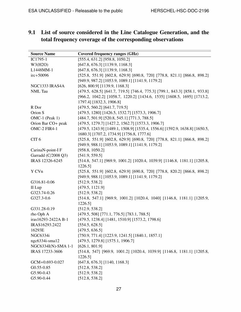
9.1 List of source considered in the Line Catalogue Generation, and thetotal frequency coverage of the corresponding observations

Source Name Covered frequency ranges (GHz)IC1795-1 [555.4, 631.2] [958.8, 1050.2]W3(H2O) [647.8, 676.3] [1139.9, 1168.3]L1448MM-1 [647.8, 676.3] [1139.9, 1168.3]irc+50096 [525.8, 551.9] [602.8, 629.9] [690.8, 720] [778.8, 821.1] [866.8, 898.2]

[949.9, 987.2] [1053.9, 1089.1] [1141.9, 1179.2]NGC1333 IRAS4A [626, 800.9] [1139.9, 1168.3]NML Tau [479.5, 628.5] [641.7, 719.5] [746.4, 775.3] [799.1, 843.3] [858.1, 933.8]

[966.2, 1042.2] [1058.7, 1220.2] [1434.6, 1535] [1608.5, 1695] [1713.2,1797.4] [1832.3, 1906.8]

R Dor [479.5, 560.2] [641.7, 719.5]Orion S [479.5, 1280] [1426.5, 1532.7] [1573.3, 1906.7]OMC-1 (Peak 1) [484.7, 501.9] [520.8, 545.1] [771.3, 788.5]Orion Bar CO+ peak [479.5, 1279.7] [1427.2, 1562.7] [1573.3, 1906.7]OMC-2 FIR4-1 [479.5, 1243.9] [1489.1, 1508.9] [1535.4, 1556.6] [1592.9, 1638.8] [1650.5,

1680.3] [1707.2, 1734.9] [1756.8, 1777.6]CIT 6 [525.8, 551.9] [602.8, 629.9] [690.8, 720] [778.8, 821.1] [866.8, 898.2]

[949.9, 988.1] [1053.9, 1089.1] [1141.9, 1179.2]CarinaN-point-I F [958.8, 1050.2]Garradd (C/2008 Q3) [541.9, 559.5]IRAS 12326-6245 [514.8, 547.1] [969.9, 1001.2] [1020.4, 1039.9] [1146.8, 1181.1] [1205.8,

1226.5]Y CVn [525.8, 551.9] [602.8, 629.9] [690.8, 720] [778.8, 820.2] [866.8, 898.2]

[949.9, 988.1] [1053.9, 1089.1] [1141.9, 1179.2]G316.81-0.06 [512.9, 538.2]II Lup [479.5, 1121.9]G323.74-0.26 [512.9, 538.2]G327.3-0.6 [514.8, 547.1] [969.9, 1001.2] [1020.4, 1040] [1146.8, 1181.1] [1205.9,

1226.5]G331.28-0.19 [512.9, 538.2]rho Oph A [479.5, 508] [771.1, 776.5] [783.1, 788.5]iras16293-2422A B-1 [479.5, 1238.4] [1481, 1510.9] [1573.2, 1798.6]IRAS16293.2422 [554.5, 628.5]16293E [479.5, 636.5]NGC6334i [750.9, 771.4] [1223.9, 1241.5] [1840.1, 1857.1]ngc6334i-sma12 [479.5, 1279.8] [1575.1, 1906.7]NGC6334I(N)-SMA 1-1 [626.1, 801.9]IRAS 17233-3606 [514.8, 547] [969.9, 1001.2] [1020.4, 1039.9] [1146.8, 1181.1] [1205.8,

1226.5]GCM+0.693-0.027 [647.8, 676.3] [1140, 1168.3]G0.55-0.85 [512.8, 538.2]G5.90-0.43 [512.9, 538.2]G5.90-0.44 [512.8, 538.2]

27

ESA UNCLASSIFIED - Releasable to the public HERSCHEL-HSC-DOC-2196

G8.14+0.23 [512.8, 538.2]G9.62+0.19 [512.8, 538.2]G8.67-0.36 [512.8, 538.2]G10.47+0.03 [514.8, 547] [969.9, 1001.2] [1020.4, 1039.9] [1146.8, 1181.1] [1205.8,

1226.5]G10.30-0.15 [512.8, 538.2]G10.34-0.14 [512.8, 538.2]G10.32-0.16 [512.8, 538.2]G10.6-0.4 (W31 C) [750.9, 771.4] [877.9, 956.1] [1108, 1232.3] [1232.5, 1238.2] [1645.1,

1678.9] [1840.1, 1857.1]GAL 12.21-0.10 [647.7, 676.3] [1139.8, 1168.3]GAL 012.91-00.2 6 [647.7, 676.3] [1139.8, 1168.3]GAL 19.61-0.23 [647.8, 676.3] [1139.8, 1168.3]G23.44-0.18 [512.8, 538.2]G24.79+0.08 [512.8, 538.2]G25.83-0.18 [512.8, 538.2]GAL 31.41+0.31 [647.8, 676.3] [1139.8, 1168.3]GAL 034.3+00.2 [647.7, 676.3] [1139.8, 1168.3]W49N [968.7, 986.9]w51-e1/e2 [1573.3, 1702.7]AFGL2591 [479.5, 1238.4]GAL79.29+00.46 [555.4, 636.0]W75N [647.8, 676.3] [1139.9, 1168.3]DR21 [968.7, 986.9] [1059.9, 1120.8] [1823.1, 1844.9]LDN1157-B1 [479.5, 1178.1] [1191.9, 1228.1] [1595.1, 1674.9]V Cyg [525.8, 551.9] [602.8, 629.9] [690.8, 720] [778.8, 821.1] [866.8, 898.2]

[949.9, 988.1] [1053.9, 1089.1] [1141.9, 1179.2]NGC7023 [521.8, 568.4] [572.2, 580.4] [1050.6, 1121.2]NGC7027 [509.5, 545.1] [556.4, 591.2] [602.8, 635.7] [670.3, 722.2] [765.5, 800.9]

[807, 850.1] [869.4, 900.1] [913.1, 944.1] [961.5, 996.4] [1022.8, 1056.5][1227.1, 1279.9] [1459.6, 1510.9] [1577, 1605] [1633.1, 1662.9] [1713.1,1739]

S CEP [525.8, 551.9] [602.8, 629.9] [690.8, 720] [778.8, 821.1] [866.8, 898.2][949.9, 988.1] [1053.9, 1089.1] [1141.9, 1179.2]

NGC7538 IRS1 [1058.7, 1116]CRL3068 [525.8, 551.9] [602.8, 629.9] [690.8, 720] [778.8, 821.1] [821.1, 866.8]

[866.8, 898.2] [949.9, 987.4] [1141.9, 1179.2]

Table 6: Frequency range of available HIFI Spectral Surveys.

28

ESA UNCLASSIFIED - Releasable to the public HERSCHEL-HSC-DOC-2196

9.2 List of observations discarded for the generation of baseline-correctedSpectral Scan and Spectral Line Catalogues

Source Observation ID Reference for supplemen-tary material

Orion KL

1342190871, 1342190872, 1342191504,1342191592, 1342191601, 1342191649,1342191725, 1342191727, 1342191728,1342191755, 1342192220, 1342192329,1342192562, 1342192563, 1342194176,1342194178, 1342194540, 1342194732,1342205334, 1342216387, 1342266895,1342192673, 1342192674, 1342194733

(5), (6), HEXOS UPDP12

SgrB2(M)

1342191482, 1342191565, 1342191680,1342192546, 1342204723, 1342204739,1342205848, 1342206455, 1342206640,1342215935, 1342216702, 1342218200,1342243701, 1342243702, 1342251112,1342192656, 1342206501, 1342266904

(4), HEXOS UPDP12

SgrB2(N)

1342204692, 1342204703, 1342204731,1342204812, 1342204829, 1342205491,1342205855, 1342206364, 1342206370,1342218198, 1342266903, 1342206498,1342206643, 1342215934, 1342216701

(12), HEXOS UPDP12

SgrB2(S) 1342190897, 1342191483, 1342191740,1342190899, 1342190900, 1342191684

HEXOS UPDP12

SgrA*

1342230279, 1342230394, 1342239594,1342239609, 1342243685, 1342243700,1342243707, 1342251185, 1342230396,1342243697, 1342243705, 1342251446,1342252173, 1342253143, 1342253145,1342266608

Goicoechea et al. in prep.

IRC+10216

1342196414, 1342196423, 1342196473,1342196475, 1342196483, 1342196514,1342196516, 1342196518, 1342196541,1342196543, 1342196566, 1342196574,1342196590, 1342210102, 1342210742,1342210754, 1342221429

(3) and upcoming UPDP

12http://archives.esac.esa.int/hsa/legacy/UPDP/HEXOS_HIFI/ReleaseNote/hexos_release_

note.pdf and http://archives.esac.esa.int/hsa/legacy/UPDP/HEXOS_HIFI/Data/

29

ESA UNCLASSIFIED - Releasable to the public HERSCHEL-HSC-DOC-2196

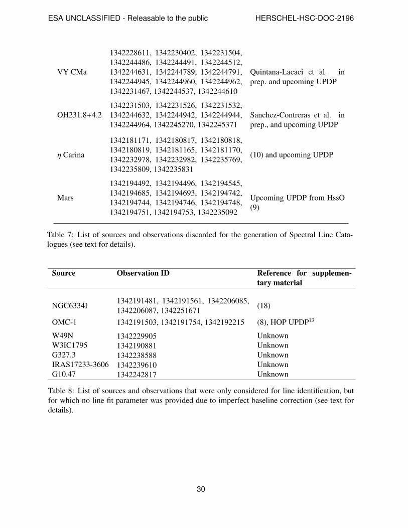
VY CMa

1342228611, 1342230402, 1342231504,1342244486, 1342244491, 1342244512,1342244631, 1342244789, 1342244791,1342244945, 1342244960, 1342244962,1342231467, 1342244537, 1342244610

Quintana-Lacaci et al. inprep. and upcoming UPDP

OH231.8+4.21342231503, 1342231526, 1342231532,1342244632, 1342244942, 1342244944,1342244964, 1342245270, 1342245371

Sanchez-Contreras et al. inprep., and upcoming UPDP

η Carina

1342181171, 1342180817, 1342180818,1342180819, 1342181165, 1342181170,1342232978, 1342232982, 1342235769,1342235809, 1342235831

(10) and upcoming UPDP

Mars

1342194492, 1342194496, 1342194545,1342194685, 1342194693, 1342194742,1342194744, 1342194746, 1342194748,1342194751, 1342194753, 1342235092

Upcoming UPDP from HssO(9)

Table 7: List of sources and observations discarded for the generation of Spectral Line Cata-logues (see text for details).

Source Observation ID Reference for supplemen-tary material

NGC6334I 1342191481, 1342191561, 1342206085,1342206087, 1342251671

(18)

OMC-1 1342191503, 1342191754, 1342192215 (8), HOP UPDP13

W49N 1342229905 UnknownW3IC1795 1342190881 UnknownG327.3 1342238588 UnknownIRAS17233-3606 1342239610 UnknownG10.47 1342242817 Unknown

Table 8: List of sources and observations that were only considered for line identification, butfor which no line fit parameter was provided due to imperfect baseline correction (see text fordetails).

30

ESA UNCLASSIFIED - Releasable to the public HERSCHEL-HSC-DOC-2196

9.3 Line parameters derived for all individual sources in the Line Cata-logue

31

ESA UNCLASSIFIED - Releasable to the public HERSCHEL-HSC-DOC-2196

Tabl

e9:

Var

ious

line

para

met

ers

deriv

edfo

ral

lind

ivid

uals

ourc

esin

the

Lin

eC

atal

ogue

.”N

/A”

indi

cate

sei

ther

that

nost

anda

rdde

viat

ion

valu

eco

uld

bede

rived

ason

lyon

etr

ansi

tion

was

repo

rted

inth

eso

urce

,or

that

the

sour

ceco

rres

pond

sto

one

ofth

ose

iden

tified

asno

tpro

vidi

ngac

cura

tefit

ted

line

flux

and

wid

th(T

able

8).

HSA

Sour

ceN

ame

RA

Dec

v 0M

edia

nv L

SR

σv L

SR

Med

ian

FWH

Mσ

FWH

MM

inFW

HM

Max

FWH

MN

bSp

ecie

sN

bTr

ansi

tions

Tota

lGH

zhh

:mm

:ss

deg:

mm

:ss

km/s

km/s

km/s

km/s

km/s

km/s

km/s

obse

rved

obse

rved

cove

red

IC17

95-1

a02

2543

.72

6206

11.4

8-3

8.90

-38.

441.

774.

433.

814.

1918

.64

935

167

W3(

H2O

)02

274.

3961

5223

.8-4

6.90

-46.

571.

315.

841.

953.

4219

.48

1897

57L

1448

MM

-1a

0325

38.8

330

445.

116.

005.

251.

541.

686.

401.

4012

.63

33

57ir

c+50

096

0326

29.4

547

3149

.17

-15.

60-1

5.29

N/A

15.7

8N

/AN

/AN

/A1

126

6N

GC

1333

IRA

S4A

a03

2910

.36

3113

31.9

87.

106.

953.

122.

3412

.56

1.85

27.2

45

520

3N

ML

Taub

0353

28.8

411

2422

.33

35.8

034

.91

0.94

21.0

16.

701.

9126

.55

1034

959

RD

or04

3645

.58

-62

0437

.35

6.00

7.66

0.56

6.64

1.02

5.01

9.22

1026

158

Ori

onS

0535

13.4

4-0

524

6.81

6.90

6.80

0.86

4.64

2.39

1.76

22.3

947

506

1240

OM

C-1

(Pea

k1)

a05

3513

.78

-05

228.

369.

608.

915.

32N

/AN

/AN

/AN

/A39

301

58O

rion

Bar

CO

+pe

ak05

3520

.73

-05

2512

.92

10.5

010

.58

0.33

2.15

0.92

1.29

10.0

129

171

1269

MW

Z90

OM

C-2

FIR

4-1

0535

27.1

3-0

509

51.3

811

.90

11.9

21.

134.

652.

961.

4520

.62

3243

093

0C

IT6a

1016

2.28

3034

19.0

1-1

.30

-1.2

22.

2518

.62

1.50

17.5

821

.91

510

267

Car

inaN

-poi

nt-I

F10

4335

.08

-59

345.

75-1

2.00

-11.

53N

/A4.

89N

/AN

/AN

/A1

191

Gar

radd

(C/2

008

Q3)

1233

48.3

7-0

553

36.4

60.

000.

03N

/A1.

22N

/AN

/AN

/A1

118

IRA

S12

326-

6245

1235

35.0

-63

0232

.16

-39.

60-3

9.58

2.14

5.84

3.71

3.05

29.7

333

181

138

YC

Vna

1245

7.84

4526

25.1

122

.30

22.4

22.

1112

.56

1.90

7.89

12.5

62

826

6G

316.

81-0

.06

1445

26.7

7-5

949

14.8

6-3

9.30

-39.

380.

574.

590.

723.

655.

564

925

IIL

up15

235.

12-5

125

58.8

1-1

4.70

-14.

343.

1125

.44

4.20

18.9

643

.16

1233

642

G32

3.74

-0.2

615

3145

.77

-56

3049

.63

-49.

60-5

0.37

0.37

5.48

1.29

4.63

8.21

57

25G

327.

3-0.

6b15

537.

85-5

437

6.58

-44.

20-4

4.29

2.62

N/A

N/A

N/A

N/A

5030

713

8G

331.

28-0

.19

1611

26.9

1-5

141

56.7

7-8

7.70

-87.

740.

956.

572.

914.

4316

.12

815

25rh

oO

phA

1626

27.7

5-2

423

55.8

63.

803.

610.

200.

960.

680.

963.

124

1839

iras

1629

3-24

22A

B-1

1632

22.6

5-2

428

33.1

23.

903.

910.

724.

812.

440.

8118

.29

4437

810

14IR

AS1

6293

-242

216

3222

.73

-24

2833

.56

4.10

3.89

1.70

4.50

3.48

2.49

16.2

719

5674

1629

3E16

3228

.47

-24

293.

143.

704.

020.

901.

290.

711.

274.

3510

2415

7N

GC

6334

I17

2053

.23

-35

4659

.14

-7.8

0-8

.23

1.47

N/A

N/A

N/A

N/A

1059

55ng

c633

4i-s

ma1

2a17

2053

.47

-35

4659

.6-7

.80

-7.9

41.

85N

/AN

/AN

/AN

/A71

2838

1132

NG

C63

34I(

N)-

SMA

1-1a

1720

55.1

8-3

545

3.9

-4.0

0-3

.95

0.67

5.06

3.08

2.49

22.2

016

108

176

IRA

S17

233-

3606

a17

2642

.51

-36

0917

.91

-2.9

0-3

.29

2.12

N/A

N/A

N/A

N/A

4323

913

8G

CM

+0.

693-

0.02

717

4721

.87

-28

2126

.69

69.8

069

.29

1.89

18.2

03.

9015

.18

24.9

77

857

G0.

55-0

.85

1750

14.5

3-2

854

30.3

416

.80

16.9

11.

186.

271.

203.

199.

8513

5125

G5.

90-0

.43

1800

40.9

2-2

404

20.1

56.

506.

640.

524.

550.

843.

886.

426

1025

G5.

90-0

.44

1800

43.9

-24

0446

.67

9.00

8.85

0.78

7.04

2.93

2.73

10.4

23

625

G8.

14+

0.23

1803

0.82

-21

489.

6920

.00

20.3

11.

334.

962.

114.

8310

.63

37

25G

9.62

+0.

1918

0614

.81

-20

3136

.77

4.42

4.23

1.48

5.92

1.90

4.29

12.9

514

3925

G8.

67-0

.36

1806

18.9

7-2

137

32.1

734

.85

34.9

10.

324.

101.

973.

189.

628

1025

G10

.47+

0.03

1808

38.2

3-1

951

50.1

966

.50

66.4

31.

71N

/AN

/AN

/AN

/A21

112

138

G10

.30-

0.15

1808

55.5

1-2

005

57.8

113

.40

13.2

10.

645.

871.

223.

507.

445

1025

G10

.34-

0.14

1808

60.0

-20

0335

.24

12.5

012

.81

0.64

4.29

4.61

2.85

12.6

33

425

G10

.32-

0.16

1809

1.5

-20

057.

5112

.40

12.5

60.

694.

411.

133.

475.

843

525

G10

.6-0

.4a

1810

28.7

1-1

955

50.7

9-2

.40

-3.0

71.

896.

952.

685.

5513

.29

817

279

GA

L12

.21-

0.10

1812

39.7

6-1

824

21.1

923

.90

24.4

90.

707.

101.

065.

7611

.35

923

57G

AL

012.

91-0

0.26

1814

39.0

-17

523.

1838

.00

37.6

30.

805.

411.

543.

7112

.53

1038

57G

AL

19.6

1-0.

2318

2738

.03

-11

5642

.47

41.1

041

.66

1.83

9.14

3.39

4.81

20.0

714

4657

G23

.44-

0.18

1834

39.1

-08

3132

.710

1.40

101.

840.

469.

933.

847.

2112

.65

22

25G

24.7

9+0.

0818

3612

.33

-07

1210

.78

111.

0711

0.97

1.11

7.02

2.06

4.14

12.6

410

2425

G25

.83-

0.18

1839

3.57

-06

2410

.35

93.8

093

.70

0.33

11.0

95.

397.

2814

.90

22

25G

AL

31.4

1+0.

3118

4734

.58

-01

1243

.07

96.9

096

.88

0.73

6.58

1.22

4.07

11.0

415

5957

GA

L03

4.3+

00.2

1853

18.5

0114

56.7

658

.50

58.5

61.

286.

272.

103.

5815

.47

2817

057

W49

Na

1910

13.2

209

0612

.04

8.00

10.2

011

.10

N/A

N/A

N/A

N/A

610

18w

51-e

1/e2

b19

2343

.76

1430

28.4

458

.44

58.7

4N

/A20

.13

N/A

N/A

N/A

11

129

AFG

L25

9120

2924

.82

4011

20.0

6-5

.50

-5.5

30.

903.

562.

162.

2816

.85

2816

675

9G

al79

.29+

00.4

620

3142

.04

4021

59.1

20.

800.

90N

/A1.

98N

/AN

/AN

/A1

181

W75

N20

3835

.92

4237

22.5

89.

409.

690.

886.

402.

124.

0315

.68

1361

57D

R21

a20

391.

0942

2249

.12

-2.6

0-2

.77

0.36

10.0

13.

465.

5715

.05

44

101

LD

N11

57-B

1a20

3910

.18

6801

9.68

-0.0

50.

271.

615.

662.

783.

2014

.65

1444

815

VC

Yg

2041

18.2

348

0828

.714

.00

14.3

20.

4413

.61

2.20

10.3

418

.13

49

267

NG

C70

23(H

2)a

2101

32.2

968

1027

.14

2.30

2.36

0.27

1.14

0.49

0.86

2.90

727

125

NG

C70

27a

2107

1.6

4214

10.4

130

.20

27.7

14.

4126

.18

6.06

19.6

336

.87

37

552

SC

EP

2135

13.2

478

3728

.78

-13.

20-1

3.94

0.53

23.5

80.

5623

.18

23.9

81

226

7N

GC

7538

IRS1

2314

16.5

161

288.

78-5

8.20

-57.

671.

034.

301.

112.

997.

717

757

CR

L30

6823

1912

.38

1711

35.7

5-3

0.60

-30.

680.

6015

.27

1.39

13.8

417

.84

36

277

aSo

urce

with

outfl

ows

bSo

urce

with

mas

ers

32