→ Herschel data for absolute beginners Herschel Science Centre (ESAC)
16
→ Herschel data for absolute beginners Herschel Science Centre (ESAC)
-
Upload
gloria-thomas -
Category
Documents
-
view
225 -
download
0
Transcript of → Herschel data for absolute beginners Herschel Science Centre (ESAC)
→
Herschel data for absolute beginners
Herschel Science Centre (ESAC)
2
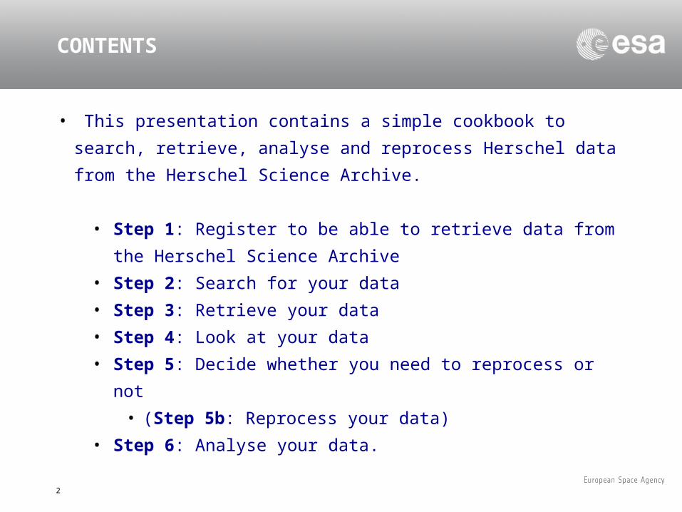
• This presentation contains a simple cookbook to search,
retrieve, analyse and reprocess Herschel data from the
Herschel Science Archive.
• Step 1: Register to be able to retrieve data from the
Herschel Science Archive
• Step 2: Search for your data
• Step 3: Retrieve your data
• Step 4: Look at your data
• Step 5: Decide whether you need to reprocess or not
• (Step 5b: Reprocess your data)
• Step 6: Analyse your data.
CONTENTS
3
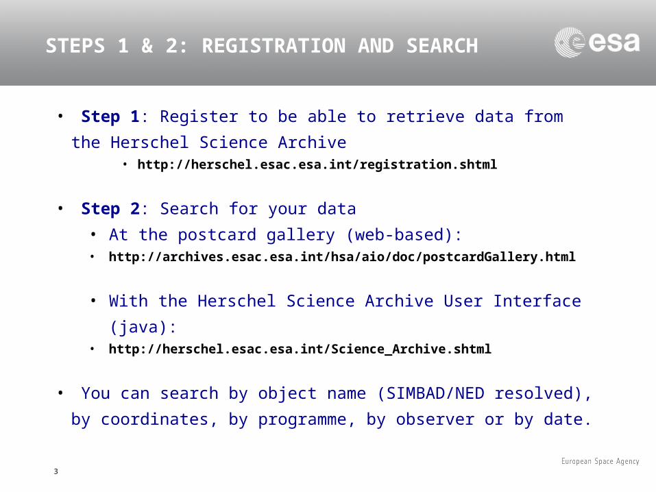
• Step 1: Register to be able to retrieve data from the Herschel
Science Archive• http://herschel.esac.esa.int/registration.shtml
• Step 2: Search for your data
• At the postcard gallery (web-based):• http://archives.esac.esa.int/hsa/aio/doc/postcardGallery.html
• With the Herschel Science Archive User Interface (java):• http://herschel.esac.esa.int/Science_Archive.shtml
• You can search by object name (SIMBAD/NED resolved), by
coordinates, by programme, by observer or by date.
STEPS 1 & 2: REGISTRATION AND SEARCH
4
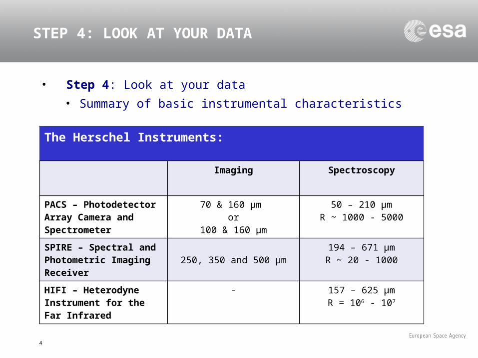
• Step 4: Look at your data
• Summary of basic instrumental characteristics
STEP 4: LOOK AT YOUR DATA
The Herschel Instruments:
Imaging Spectroscopy
PACS – Photodetector Array Camera and Spectrometer
70 & 160 μm or
100 & 160 μm
50 – 210 μmR ~ 1000 - 5000
SPIRE – Spectral and Photometric Imaging Receiver
250, 350 and 500 μm194 – 671 μmR ~ 20 - 1000
HIFI – Heterodyne Instrument for the Far Infrared
- 157 – 625 μmR = 106 - 107
5
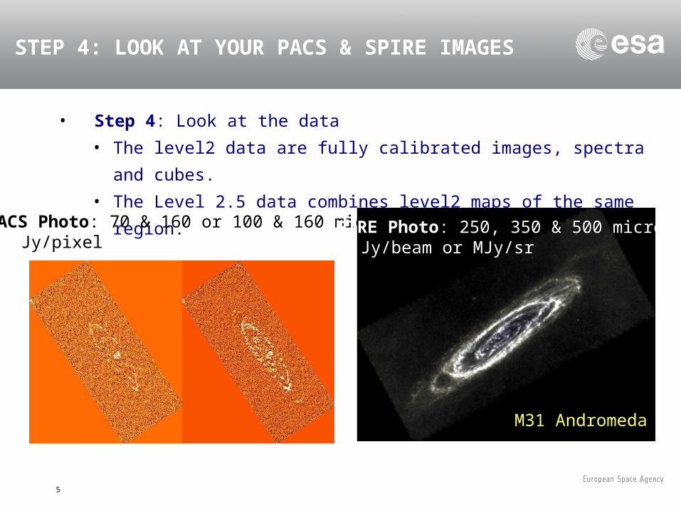
• Step 4: Look at the data
• The level2 data are fully calibrated images, spectra and cubes.
• The Level 2.5 data combines level2 maps of the same region.
STEP 4: LOOK AT YOUR PACS & SPIRE IMAGES
PACS Photo: 70 & 160 or 100 & 160 micronJy/pixel
SPIRE Photo: 250, 350 & 500 micronsJy/beam or MJy/sr
M31 Andromeda
6
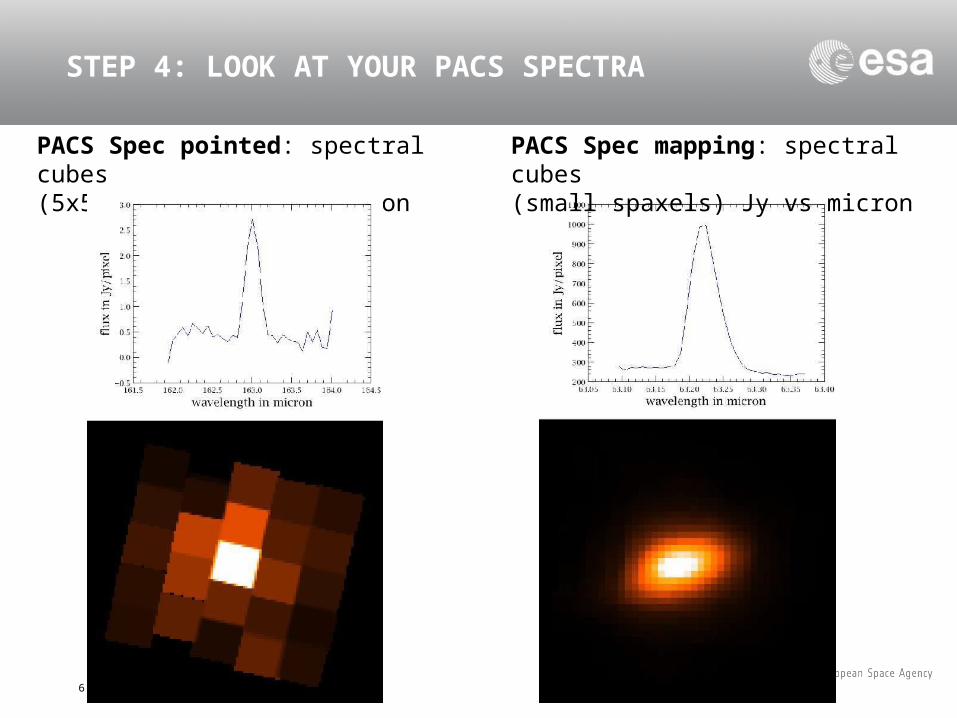
STEP 4: LOOK AT YOUR PACS SPECTRA
PACS Spec pointed: spectral cubes (5x5 spaxels) Jy vs micron
PACS Spec mapping: spectral cubes (small spaxels) Jy vs micron
7
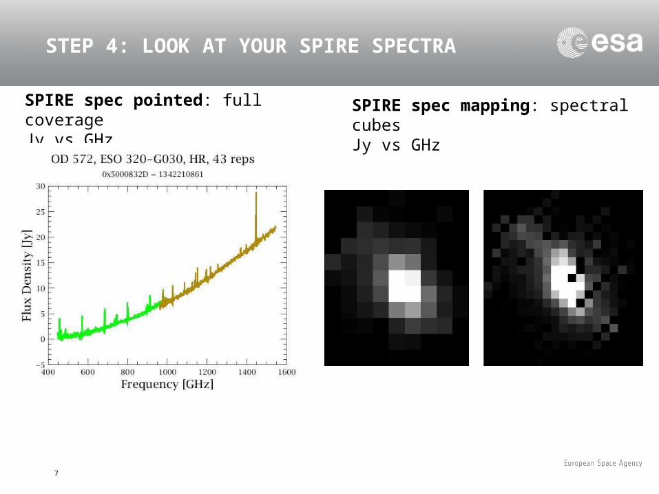
STEP 4: LOOK AT YOUR SPIRE SPECTRA
SPIRE spec pointed: full coverageJy vs GHz
SPIRE spec mapping: spectral cubesJy vs GHz
8
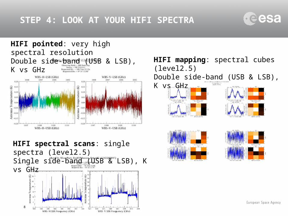
STEP 4: LOOK AT YOUR HIFI SPECTRA
HIFI pointed: very high spectral resolutionDouble side-band (USB & LSB), K vs GHz
HIFI mapping: spectral cubes (level2.5)Double side-band (USB & LSB), K vs GHz
HIFI spectral scans: single spectra (level2.5)Single side-band (USB & LSB), K vs GHz
9
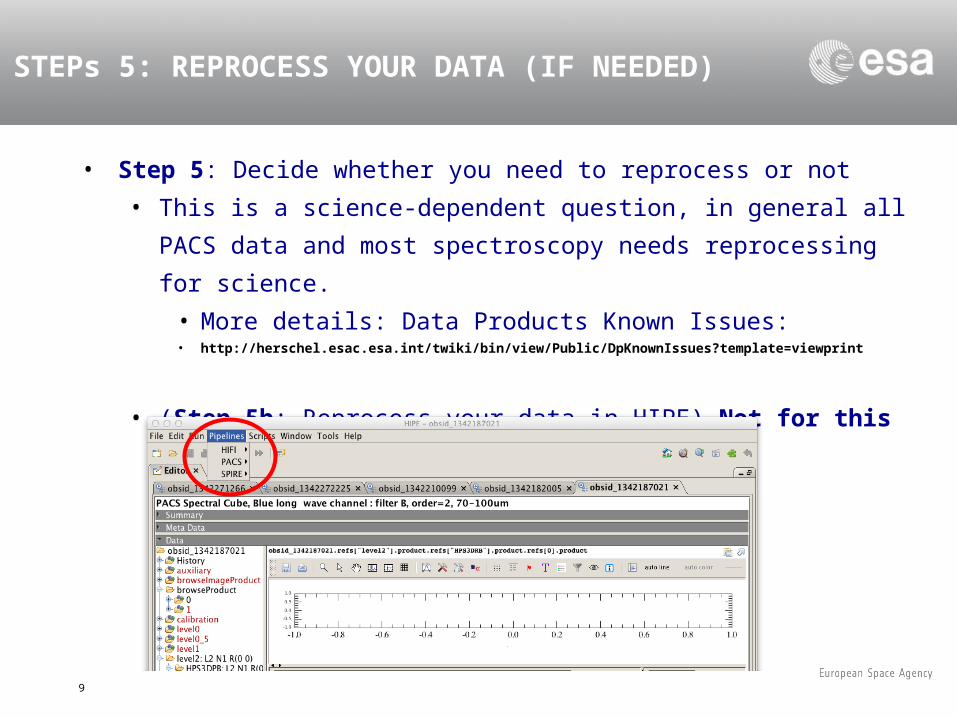
• Step 5: Decide whether you need to reprocess or not
• This is a science-dependent question, in general all PACS data
and most spectroscopy needs reprocessing for science.
• More details: Data Products Known Issues:• http://herschel.esac.esa.int/twiki/bin/view/Public/DpKnownIssues?template=viewprint
• (Step 5b: Reprocess your data in HIPE) Not for this demo
STEPs 5: REPROCESS YOUR DATA (IF NEEDED)
10
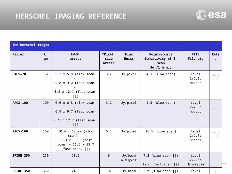
The Herschel Images
Filter λ μm
FWHM arcsec
“Pixel” size
arcsec
FluxUnits
Point-source Sensitivity mini-
scan5σ /1 h mJy
FITSFilename
Refs.
PACS–70 70 5.2 x 5.8 (slow scan) – 5.8 x 9.0 (fast scan) –
5.8 x 12.1 (fast scan, ||)
3.2 Jy/pixel 4.7 (slow scan) Level 2/2.5: hppppb
1, 2, 3
PACS-100 100 6.6 x 6.8 (slow scan) – 6.9 x 9.7 (fast scan) –
6.9 x 12.7 (fast scan, ||)
3.2 Jy/pixel 5.5 (slow scan) Level 2/2.5: hppppb
1, 2, 3
PACS-160 160 10.4 x 12.02 (slow scan) - 11.3 x 13.3 (fast scan) – 11.6 x 15.7 (fast scan, ||)
6.4 Jy/pixel 10.5 (slow scan) Level 2/2.5: hppppr
1, 2, 3
SPIRE-250 250 18.2 6 Jy/beam& MJy/sr
7.3 (slow scan ||) – 12.6 (fast scan ||)
Level 2/2.5: Hspirepsw
4
SPIRE-350 350 24.9 10 Jy/beam& MJy/sr
6.0 (slow scan ||) – 10.5 (fast scan ||)
Level 2/2.5: hspirepmw
4
SPIRE-500 500 36.3 14 Jy/beam& Mjy/sr
8.7 (slow scan ||) – 15.0 (fast scan ||)
Level 2/2.5: Hspireplw
4
HERSCHEL IMAGING REFERENCE
11
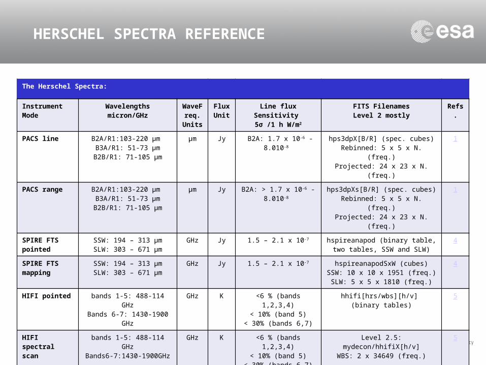
The Herschel Spectra:
Instrument Mode
Wavelengthsmicron/GHz
WaveFreq.Units
Flux Unit
Line flux Sensitivity 5σ /1 h W/m2
FITS FilenamesLevel 2 mostly
Refs.
PACS line B2A/R1:103-220 μm B3A/R1: 51-73 μm
B2B/R1: 71-105 μm
μm Jy B2A: 1.7 x 10⁻⁶ - 8.010-8
hps3dpX[B/R] (spec. cubes)Rebinned: 5 x 5 x N. (freq.)
Projected: 24 x 23 x N. (freq.)
1
PACS range B2A/R1:103-220 μm B3A/R1: 51-73 μm
B2B/R1: 71-105 μm
μm Jy B2A: > 1.7 x 10⁻⁶ - 8.010-8
hps3dpXs[B/R] (spec. cubes)Rebinned: 5 x 5 x N. (freq.)
Projected: 24 x 23 x N. (freq.)
1
SPIRE FTS pointed
SSW: 194 – 313 μmSLW: 303 – 671 μm
GHz Jy 1.5 – 2.1 x 10⁻⁷ hspireanapod (binary table, two tables, SSW and SLW)
4
SPIRE FTS mapping
SSW: 194 – 313 μmSLW: 303 – 671 μm
GHz Jy 1.5 – 2.1 x 10⁻⁷ hspireanapodSxW (cubes)SSW: 10 x 10 x 1951 (freq.)
SLW: 5 x 5 x 1810 (freq.)
4
HIFI pointed bands 1-5: 488-114 GHzBands 6-7: 1430-1900
GHz
GHz K <6 % (bands 1,2,3,4)< 10% (band 5)
< 30% (bands 6,7)
hhifi[hrs/wbs][h/v] (binary tables)
5
HIFI spectral scan
bands 1-5: 488-114 GHzBands6-7:1430-1900GHz
GHz K <6 % (bands 1,2,3,4)< 10% (band 5)
< 30% (bands 6,7)
Level 2.5: mydecon/hhifiX[h/v]WBS: 2 x 34649 (freq.)
5
HIFI mapping bands 1-5: 488-114 GHzBands6-7:1430-1900GHz
GHz K <6 % (bands 1,2,3,4)< 10% (band 5)
< 30% (bands 6,7)
Level 2.5: hhifiX[h/v] [lsb/usb] HRS: 5 x 29 x 3826 (cubes)WBS: 5 x 29 x 1128 (cubes)
5
HERSCHEL SPECTRA REFERENCE
12
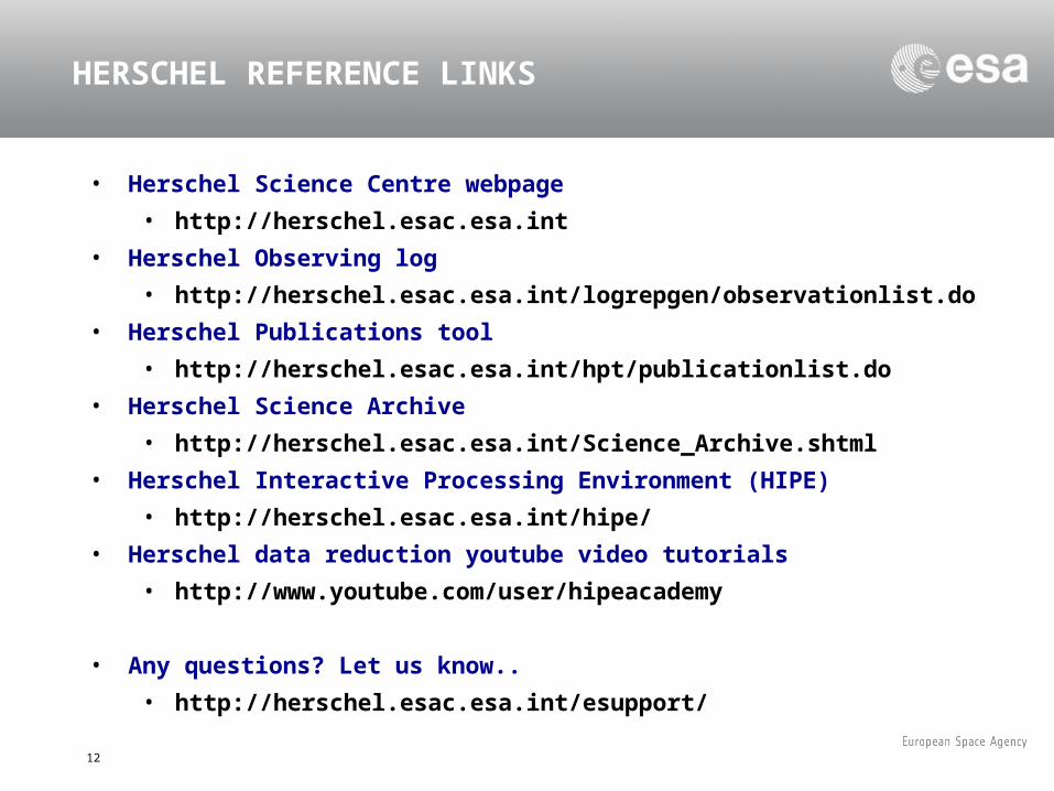
HERSCHEL REFERENCE LINKS
• Herschel Science Centre webpage
• http://herschel.esac.esa.int
• Herschel Observing log
• http://herschel.esac.esa.int/logrepgen/observationlist.do
• Herschel Publications tool
• http://herschel.esac.esa.int/hpt/publicationlist.do
• Herschel Science Archive
• http://herschel.esac.esa.int/Science_Archive.shtml
• Herschel Interactive Processing Environment (HIPE)
• http://herschel.esac.esa.int/hipe/
• Herschel data reduction youtube video tutorials
• http://www.youtube.com/user/hipeacademy
• Any questions? Let us know..
• http://herschel.esac.esa.int/esupport/
13
Thank youAny questions?
14
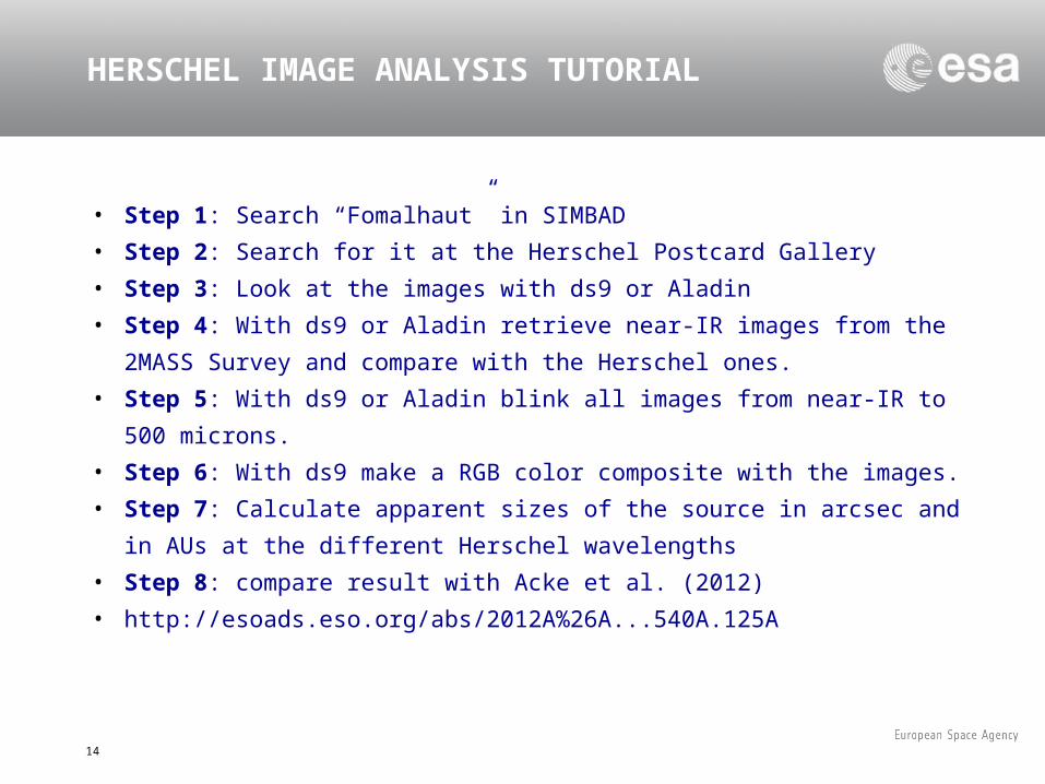
• Step 1: Search “Fomalhaut” in SIMBAD
• Step 2: Search for it at the Herschel Postcard Gallery
• Step 3: Look at the images with ds9 or Aladin
• Step 4: With ds9 or Aladin retrieve near-IR images from the 2MASS Survey
and compare with the Herschel ones.
• Step 5: With ds9 or Aladin blink all images from near-IR to 500 microns.
• Step 6: With ds9 make a RGB color composite with the images.
• Step 7: Calculate apparent sizes of the source in arcsec and in AUs at the
different Herschel wavelengths
• Step 8: compare result with Acke et al. (2012)
• http://esoads.eso.org/abs/2012A%26A...540A.125A
HERSCHEL IMAGE ANALYSIS TUTORIAL

15
• From parallax to parsec:
• Distance(parsec) = 1./AngularSize(arcsec)
• From angular size to physical size
• Distance (AU) = Distance (parcsec) * AngularSize (arcsec)
HERSCHEL IMAGE ANALYSIS TUTORIAL
16
• Feedback forum:
• http://mmi-forum.wikispaces.com/home
ABOUT THE MULTIMISSION INTERFACE