HIFI Observers' Manualherschel.esac.esa.int/Docs/HIFI/pdf/hifi_om.pdf · HIFI Observers' Manual...
117
HIFI Observers' Manual Update for Start of OT2 Call for Proposals HERSCHEL-HSC-DOC-0784, version 2.4 1-June-2011
Transcript of HIFI Observers' Manualherschel.esac.esa.int/Docs/HIFI/pdf/hifi_om.pdf · HIFI Observers' Manual...
HIFI Observers' Manual
Update for Start of OT2 Call for Proposals
HERSCHEL-HSC-DOC-0784, version 2.41-June-2011
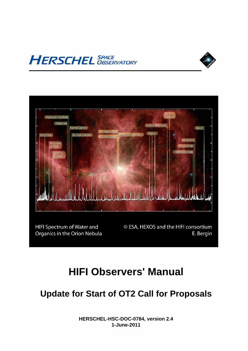
Cover image: A single sideband spectrum covering the whole of one subbandof HIFI towards the Orion nebula, superimposed on a Spitzer Space Telescope
colour composite of the region from IRAC and MIPS images (Credit: NASA).
HIFI Observers' Manual:
Update for Start of OT2 Call for Proposals
Published version 2.4, 1-June-2011Copyright © 2011
Revision History
Revision version 2.4 APM, DT
Update for changes made for the OT2 call including in-flight calibration information updates.
Revision version 2.3 APM, DT
Update for changes made for the GT2 call including HSpot 5.3 updates.
Revision version 2.2 APM, DT
Update for changes made for the GT2 call
Revision version 2.1 APM, DT
Update for changes made starting OT1 observations
Revision version 2.0 APM, DT
Update for initial Open Time call (OT1)
Revision version 1.1 APM, DT
Update for initial Open Time Key Projects
Revision version 1.0 APM, DT
Initial version
iv
Table of Contents1. The HIFI Instrument Observer's Manual ........................................................................ 1
1.1. Purpose of this Document ................................................................................ 11.2. Preparing HIFI for Operations ........................................................................... 11.3. Acknowledgements ......................................................................................... 2
2. HIFI Instrument Description ........................................................................................ 32.1. Instrument and Concept ................................................................................... 3
2.1.1. What is HIFI? ...................................................................................... 32.1.2. How Does HIFI Work? ......................................................................... 3
2.2. Instrument Configuration .................................................................................. 52.3. HIFI Focal Plane Unit ..................................................................................... 6
2.3.1. The Common Optics Assembly ............................................................... 72.3.2. The Beam Combiner Assembly (Diplexer Unit) ......................................... 82.3.3. HIFI Mixers ........................................................................................ 92.3.4. The Focal Plane Chopper ..................................................................... 102.3.5. The Calibration Source Assembly .......................................................... 11
2.4. The HIFI Signal Chain ................................................................................... 112.5. HIFI Spectrometers ....................................................................................... 12
2.5.1. The Wide Band Spectrometer (WBS) ..................................................... 122.5.2. The High Resolution Spectrometer (HRS) ............................................... 13
3. HIFI Scientific Capabilities and Performance ................................................................ 153.1. What Science Is Possible With HIFI? ............................................................... 15
3.1.1. HIFI's Scientific Objectives .................................................................. 153.2. Primary Instrument Characteristics ................................................................... 163.3. General Instrument Description ........................................................................ 173.4. Available Spectrometer Setups ....................................................................... 18
3.4.1. Wide Band Spectrometers (WBSs) ......................................................... 183.4.2. High Resolution Spectrometers (HRSs) ................................................... 18
3.5. Mixer Performance ........................................................................................ 193.5.1. System Temperatures ........................................................................... 193.5.2. Tuning Ranges ................................................................................... 203.5.3. Sensitivity Variations Across the IF Band ................................................ 233.5.4. Overall Noise Performance ................................................................... 243.5.5. Mixer Stabilities ................................................................................. 25
4. Observing with HIFI ................................................................................................ 274.1. Introduction .................................................................................................. 274.2. The HIFI Observing Modes ............................................................................ 27
4.2.1. Modes of the Single Point AOT I .......................................................... 284.2.2. Modes of the Mapping AOT II .............................................................. 364.2.3. Modes of the Spectral Scan AOT III ...................................................... 41
4.3. Standing Wave Residuals after Calibration (Pipeline Level 2) ................................ 444.3.1. Bands 1-5 (SIS mixers) ........................................................................ 444.3.2. Position Switch, Frequency Switch and Load Chop modes .......................... 46
4.4. Bands 6-7 (HEB mixers) ................................................................................ 474.4.1. DBS Modes ....................................................................................... 474.4.2. Position Switch, Frequency Switch and Load Chop Modes .......................... 48
4.5. "Grouping" or "Clustering" of Observations ....................................................... 484.6. Solar System Target Modes ............................................................................ 48
5. HIFI Calibration ...................................................................................................... 495.1. Introduction: ................................................................................................. 495.2. The Intensity Calibration of HIFI ..................................................................... 49
5.2.1. Context ............................................................................................. 495.3. The HIFI Calibration Scheme .......................................................................... 49
5.3.1. Internal Load Calibrations .................................................................... 495.3.2. OFF calibration .................................................................................. 515.3.3. Differencing observations: .................................................................... 52
HIFI Observers' Manual
v
5.3.4. Non-linearity: ..................................................................................... 525.3.5. Blank-sky contribution: ........................................................................ 525.3.6. Conversion between Antenna Temperature and Janskys: ............................. 52
5.4. The Frequency Calibration of HIFI: .................................................................. 525.4.1. Context: ............................................................................................ 535.4.2. Frequency accuracy: ............................................................................ 535.4.3. Determination of Frequency Calibration: ................................................. 535.4.4. Frequency resolution: .......................................................................... 535.4.5. Frequency and Velocity Verifications ..................................................... 545.4.6. Spurious Responses in HIFI .................................................................. 55
5.5. The Spatial Response Calibration of HIFI: ......................................................... 595.5.1. Context: ............................................................................................ 595.5.2. Beam Characteristics ........................................................................... 605.5.3. Chopper Calibration ............................................................................ 68
5.6. Mixer Side-band Ratio ................................................................................... 695.6.1. IF Spectrum Repeatability (Sideband Line Ratios) ..................................... 695.6.2. Summary Sideband Ratio Information .................................................... 715.6.3. Intrinsic sideband ratio IF dependence .................................................... 72
5.7. Summary: overall calibration of HIFI and error budget: ........................................ 735.7.1. Strategy summary: .............................................................................. 735.7.2. Error budget ...................................................................................... 73
6. Using HSpot to Create HIFI Observations ................................................................... 746.1. Overview .................................................................................................... 746.2. HSpot Components for Setting Up a HIFI Observation ......................................... 74
6.2.1. Working with A HIFI Pointed or Mapping Observation Template ................. 746.2.2. HIFI Spectral Scan AOT ...................................................................... 82
6.3. Example HIFI Single Point Observation Setups .................................................. 856.3.1. Example 1: Observing the [CII] line using Frequency Switch in a photodis-sociation region ........................................................................................... 866.3.2. Example 2: A Dual Beam Switch (DBS) mode AGB Observation ................. 92
6.4. Example Setup of a HIFI Mapping AOR ........................................................... 976.4.1. Example 3: Scan Mapping of the Spectral Lines CO(7-6) and CI(2-1) in theCentre of M51 . .......................................................................................... 97
6.5. Example Setup of a HIFI Spectral Scan Observation .......................................... 1016.5.1. Example 4: Spectral Survey of a Hot Core. ............................................ 101
7. Pipeline and Data Products Description ..................................................................... 1047.1. Data to be Passed on to the User .................................................................... 1047.2. Additional Observatory Meta Data .................................................................. 1047.3. Example HIFI data products .......................................................................... 104
7.3.1. Level 0 products ............................................................................... 1047.3.2. Level 1 products ............................................................................... 105
7.4. Pipeline Processing ...................................................................................... 1067.4.1. WBS Pipeline Processing Steps ........................................................... 1067.4.2. HRS Pipeline Processing Steps ............................................................ 107
7.5. Deconvolution Processing of Spectral Scan Data ............................................... 1077.5.1. Solving the Deconvolution Problem ...................................................... 108
8. References: ........................................................................................................... 110A. Change Log ......................................................................................................... 111
A.1. ................................................................................................................ 111
1
Chapter 1. The HIFI InstrumentObserver's Manual1.1. Purpose of this Document
The HIFI (Heterodyne Instrument for the Far Infrared) observer's manual is intended to assist in usingthe HIFI instrument on board ESA's Herschel Space Observatory. Documents on the detailed docu-ments on design and operations are available from the Herschel Science Centre (HSC) and the HIFIInstrument Control Centre at SRON, Groningen, The Netherlands (HIFI ICC -- who are responsiblefor the safety and calibration of HIFI during operations).
Help and information on HIFI can be obtained by contacting the Herschel Science Centre at the fol-lowing web address:
http://herschel.esac.esa.int
Follow the link on the page to the "Helpdesk" for problem enquiries.
This document contains overview information on instrument concept and design, its scientific perfor-mance and calibration. It also contains all user-relevant information on observing modes and Astro-nomical Observing Templates (AOTs) Examples of AOTs for HIFI are presented with their usage.
HIFI data from the Herschel Space Observatory are automatically processed at the HSC after the datais received from the spacecraft. The standard processing - pipeline - is described here together witha description of the data products. Both the raw and pipeline processed data are made available tothe user.
Finally, a brief mention is made of software tools that have been more specifically provided for thekinds of sophisticated analysis that is likely to be needed for HIFI data reduction. These will avail-able to the user through the Herschel Common Science System, which will be made available by theHerschel Science Centre. It should be noted that all pipeline software modules are available to usersvia installation of the Herschel Common Science System. Reprocessing of data can therefore be per-formed with pipeline, or adapted pipeline, scripts by users on their own workstations.
1.2. Preparing HIFI for OperationsIn August 2009, a sequence of events triggered by a corruption of on-board memory lead to the lossof the prime side electronics chain of HIFI. Since then, a significant effort has been made that hasenabled a full recovery of the instrument using its redundant side electronics.
The special circumstances of HIFI's switch to redundant side operations, and resuming with a com-pressed Performance Verification phase and accelerated Observing Mode release, has involved thesupport of many others, together with the HIFI Calibration Scientists and Instrument Engineers. Thisincludes KP team apprentices who have been variously present at the HIFI ICC in the Fall of 2009and during the performance verification phase starting end-January 2010, and also the HIFI softwaredevelopment team who have been available at all times. AOT test planning has been done in consul-tation with the KP PIs coordinated by X. Tielens, Instrument P.I. F. Helmich, Project Manager P.Roelfsema, and with the Mission Scientist J. Cernicharo. These persons should be acknowledged, ashaving directly supported the flight qualification of HIFI as a science instrument.
AOT/Uplink Engineering Team: P. Morris (Caltech), M. Olberg (SRON/Chalmers), V. Ossenkopf(U. Köln), C. Risacher (SRON), D. Teyssier (HSC/ESA).
Instrument Engineers and System Architects: P. Dieleman (SRON), K. Edwards (SRON), W. Jelle-ma (SRON), A. de Jonge (SRON), W. Laauwen (SRON), J. Pearson (JPL).
The HIFI Instrument Observer's Manual
2
HIFI Calibration Scientists: I. Avruch (Kapteyn/SRON), A. Boogert (Caltech), C. Borys (Caltech),J. Braine (U. Bordeaux), F. Herpin (U. Bordeaux), R. Higgins (U. Maynooth), S. Lord (Caltech), A.Marston (HSC/ESA) C. McCoey (U. Waterloo), R. Moreno (Obs. Paris), M. Rengel (MPS)
HIFI Software Development Team: R. Assendorp (SRON), B. Delforge (SRON), A. Hoac (Cal-tech), D. Kester (SRON), A. Lorenzani (Obs. Acetri), M. Melchior (U. Appl. Sci. NW Switzerland),W. Salomons (SRON), B. Thomas (SRON), E. Sanchez (CSIC), R. Shipman (SRON), Y. Poelman(SRON), J. Xie (Caltech), P. Zaal (SRON)
HIFI KP student/postdoc visitors: E. DeBeck (U. Leuven), T. Bell (Caltech), N. Crockett (U. Michi-gan), P. Bjerkeli (Chalmers), P. Hily-Blant (Obs. Grenoble), M. Kama (U. Amsterdam), T. Kaminski(CAMK), B. Larsson (Obs. Stockholm), B. Lefloch (Obs. Grenoble), R. Lombaert (U. Leuven), M.de Luca (Obs. Paris), Z. Makai (U. Köln), M. Marseille (SRON), Z. Nagy (Kapteyn), Y. Okada (U.Köln), S. Pacheco (Obs. Grenoble), D. Rabois (U. Toulouse), Frank Schlöder (U. Köln), S. Wang (U.Michigan), M. van der Wiel (Kapteyn/SRON), M. Yabaki (U. Köln), U. Yildiz (U. Leiden)
HIFI KP PI Representatives to the ICC/AOT Team: E. Caux (U. Toulouse), E. van Dishoek (U.Leiden), M. Gerin (Obs. Grenoble)
1.3. AcknowledgementsThe HIFI instrument is the result of many years of work by a large group of dedicated people. It istheir efforts that have made it possible to create such a powerful heterodyne instrument for use in theHerschel Space Observatory. We would first like to acknowledge their work.
The manual itself included help and inputs from a number of people. Particular help and contributionsto this manual have come from the calibration group and recent in-orbit calibration updates they haveprovided. In particular, the following people have made significant contributions
• Anthony Marston (ESAC, editor), 1 June 2011.
• David Teyssier (ESAC)
• Christophe Risacher (SRON)
• Patrick Morris (NHSC)
• Michael Olberg (Onsala)
• Volker Ossenkopf (U. Köln)
3
Chapter 2. HIFI InstrumentDescription2.1. Instrument and Concept2.1.1. What is HIFI?
HIFI is the Heterodyne Instrument for the Far Infrared. It is designed to provide spectroscopy at high tovery high resolution over a frequency range of approximately 480-1250 and 1410-1910 GHz (625-240and 213-157 microns). This frequency range is covered by 7 "mixer" bands, with dual horizontal andvertical polarizations, which can be used one pair at a time (see Table 3.1 for detailed specification).
The mixers act as detectors that feed either, or both, the two spectrometers on HIFI. An instantaneousfrequency coverage of 2.4GHz is provided with the high frequency band 6 and 7 mixers, while forbands 1 to 5 a frequency range of 4GHz is covered. The data is obtained as dual sideband data whichmeans that each channel of the spectrometers reacts to two frequencies (separated by 4.8 to 16 GHz)of radiation at the same time (see Section 2.1.2 and Section 3.1). For many situations, this overlap-ping of frequencies is not a major problem and science signals are clearly distinguishable. However,particularly for complex sources containing a high density of emission/absorption lines, this can leadto problems with data interpretation. Deconvolution is therefore necessary for the data to create sin-gle sideband data. This is especially important for spectral scans covering large frequency ranges onsources with many lines (see Chapter 6).
There are four spectrometers on board HIFI, two Wide-Band Acousto-Optical Spectrometers (WBS)and two High Resolution Autocorrelation Spectrometers (HRS). One of each spectrometer type isavailable for each polarization. They can be used either individually or in parallel. The Wide-BandSpectrometers cover the full intermediate frequency bandwidth of 2.4GHz in the highest frequencybands (bands 6 and 7) and 4GHz in all other bands. The High Resolution Spectrometers have variableresolution with subbands sampling up to half the 4GHz intermediate frequency range. Subbands havethe flexibility of being placed anywhere within the 4GHz range.
2.1.2. How Does HIFI Work?Sub-mm continuum radiation is best detected with bolometers, which act like thermometers, measur-ing the heat coming in and translating it to integrated intensities. Line radiation is much more difficultto detect. There are no amplifiers available to amplify the weak sky signals at sub-millimeter wave-lengths. For lower frequencies there are, however, good amplifiers available, which can be small, lowin energy consumption and weight. These are thus very suitable for a space observatory.
2.1.2.1. The Mixers
The solution is thus to bring the signal down in frequency, without losing its information content. Thisis accomplished, through heterodyne techniques in which the sky signal is mixed with another signal(Local Oscillator) very close to the frequency of interest. In performing such mixing of signals, theresulting signal is of much lower frequency, while still having all the spectral detail of the originalsky-signal. Modern mixing devices such as SIS (semiconductor-insulator-semiconductor) mixers orhot electron bolometer (HEB) mixers, not only perform the mixing but can also amplify the signal,making them eminently suitable for instruments like HIFI.
Mixing: The mixers used by HIFI are at superconducting temperatures (the HEBs are on the borderof normal and superconducting). They are non-linear devices in that the current out is not directlyproportional to the voltage across them -- in fact their current-voltage curves have similarities to thoseof diodes. This allows amplification of the mixed signals of the incoming radiation and an on-boardlocal oscillator. In particular, the "beat" frequency ( | fs - fLO | ) between each of the incoming sourcefrequencies, fs, and the single Local Oscillator frequency, fLO.
HIFI Instrument Description
4
Intermediate Frequency: The "beat" frequencies produce the so-called Intermediate Frequency (IF) ofthe instrument. Further amplification is made of these intermediate frequencies and, for HIFI, filteringallows the detection of IFs of 4 to 8GHz which is done in the HIFI spectrometers.
2.1.2.2. Double Sideband Data
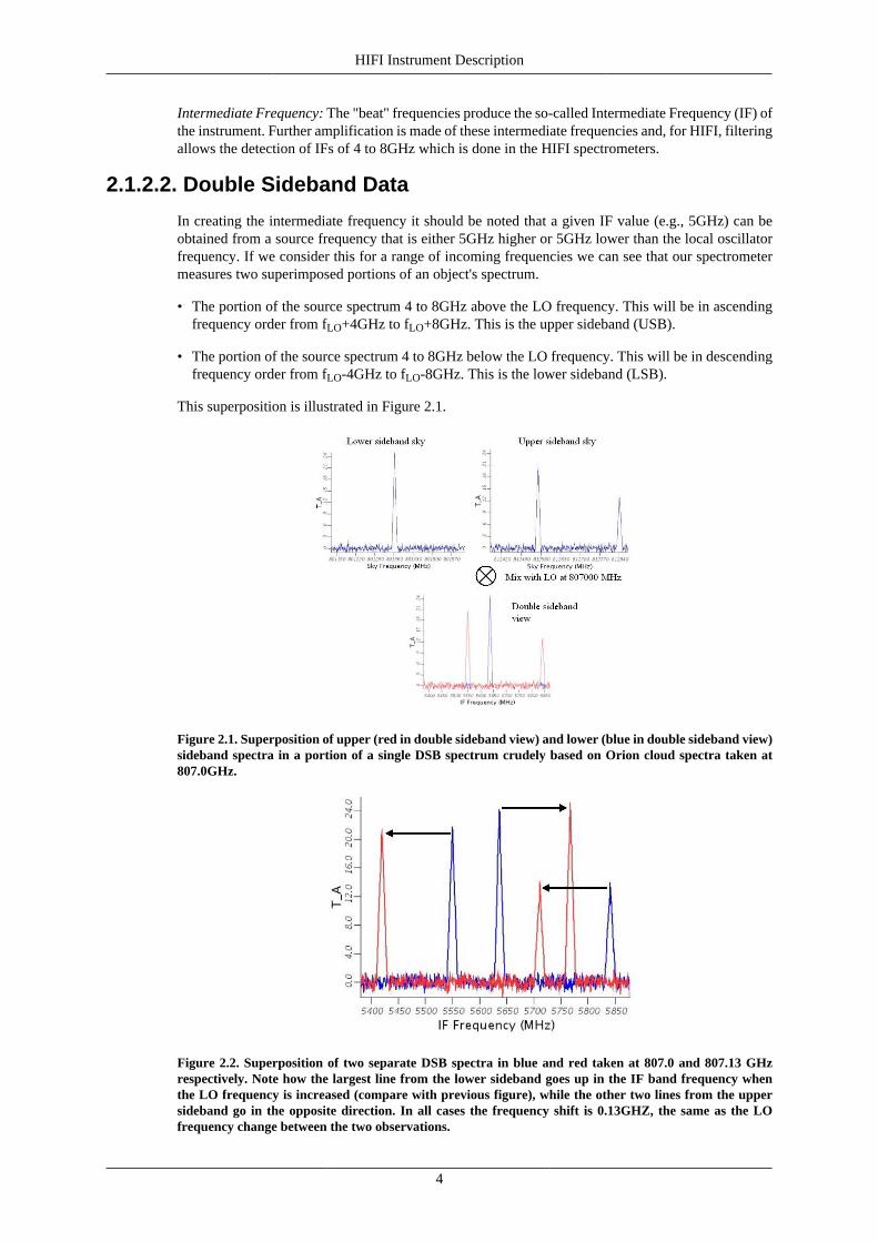
In creating the intermediate frequency it should be noted that a given IF value (e.g., 5GHz) can beobtained from a source frequency that is either 5GHz higher or 5GHz lower than the local oscillatorfrequency. If we consider this for a range of incoming frequencies we can see that our spectrometermeasures two superimposed portions of an object's spectrum.
• The portion of the source spectrum 4 to 8GHz above the LO frequency. This will be in ascendingfrequency order from fLO+4GHz to fLO+8GHz. This is the upper sideband (USB).
• The portion of the source spectrum 4 to 8GHz below the LO frequency. This will be in descendingfrequency order from fLO-4GHz to fLO-8GHz. This is the lower sideband (LSB).
This superposition is illustrated in Figure 2.1.
Figure 2.1. Superposition of upper (red in double sideband view) and lower (blue in double sideband view)sideband spectra in a portion of a single DSB spectrum crudely based on Orion cloud spectra taken at807.0GHz.
Figure 2.2. Superposition of two separate DSB spectra in blue and red taken at 807.0 and 807.13 GHzrespectively. Note how the largest line from the lower sideband goes up in the IF band frequency whenthe LO frequency is increased (compare with previous figure), while the other two lines from the uppersideband go in the opposite direction. In all cases the frequency shift is 0.13GHZ, the same as the LOfrequency change between the two observations.
HIFI Instrument Description
5
2.1.2.3. Consequences of Double Sideband (DSB) Data
For a number of regions where a single strong line of known frequency is the subject of study, knowingwhether it is in the upper or lower sideband frequency range is easy to determine - and so it is easyto assign the correct frequency to the spectrum scale.
Small LO shifts: However, for cases where it is not known a priori which spectral lines are in whichsideband the simplest way to determine this is by shifting the LO frequency. An increase in LO fre-quency will lead to USB features moving to lower IF frequencies and LSB features moving to higher IFfrequencies (see Figure 2.2). It then becomes clear which sideband (and frequency) the features are in.
Deconvolution: Even the above technique becomes impossible for regions where there is a high den-sity of spectral features. In such cases, the chances become quite high that USB features and LSBfeatures will overlap. And the shifting of the LO may only lead to other feature overlaps. For this casedeconvolution techniques have been devised (see Chapter 7). These allow large regions of frequencyspace to be sampled by many positionings of the LO frequency. A reconstruction of the spectrum(single sideband, SSB) can then be made.
2.1.2.4. The HIFI Flux Units: Antenna Temperature
Sub-mm astronomy derives many of its units from radio astronomy. The standard unit for measuringthe power received is antenna temperature, TA, which is defined by:
kTA = power received per unit frequency
If the intensity is constant across the whole beam then the antenna temperature is equivalent to thebrightness temperature (the temperature a blackbody needs to be in order to see the observed intensityat a given frequency).
This is a particularly convenient scale to use since flux calibration is made by comparison of the sourcemeasurement with measurements of hot and cold blackbody loads internal to HIFI.
However, sources do not usually fill any of the HIFI beams and a correction, usually in the form of anaperture efficiency, is needed. For more details on the calibration procedure see Chapter 5.
The main noise contribution for measurements is from to the instrument itself. This noise level isreferred to as the system temperature, Tsys
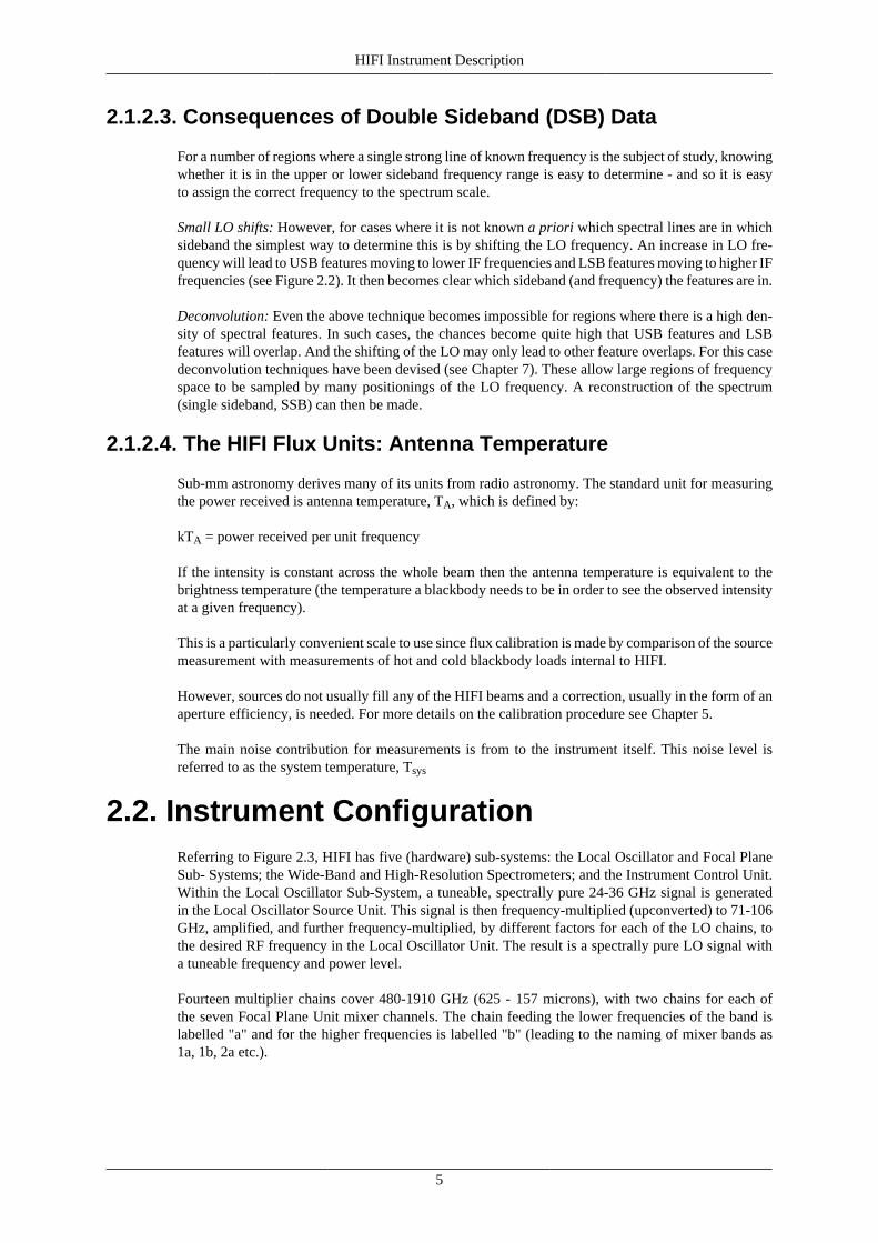
2.2. Instrument ConfigurationReferring to Figure 2.3, HIFI has five (hardware) sub-systems: the Local Oscillator and Focal PlaneSub- Systems; the Wide-Band and High-Resolution Spectrometers; and the Instrument Control Unit.Within the Local Oscillator Sub-System, a tuneable, spectrally pure 24-36 GHz signal is generatedin the Local Oscillator Source Unit. This signal is then frequency-multiplied (upconverted) to 71-106GHz, amplified, and further frequency-multiplied, by different factors for each of the LO chains, tothe desired RF frequency in the Local Oscillator Unit. The result is a spectrally pure LO signal witha tuneable frequency and power level.
Fourteen multiplier chains cover 480-1910 GHz (625 - 157 microns), with two chains for each ofthe seven Focal Plane Unit mixer channels. The chain feeding the lower frequencies of the band islabelled "a" and for the higher frequencies is labelled "b" (leading to the naming of mixer bands as1a, 1b, 2a etc.).
HIFI Instrument Description
6
Figure 2.3. General HIFI component diagram.
The local oscillator beams are fed into the Focal Plane Unit through 7 windows in the Herschel cryostat.Within the Focal Plane Unit, the astronomical signal from the telescope is split into 7 beams. Each ofthese signal beams is combined with its corresponding LO beam, and then split into 2 linearly polarizedbeams that are focused into 2 mixer units. Each mixer unit generates an intermediate frequency (IF)signal that is amplified prior to leaving the Focal Plane Unit.
The IF output signals from the Focal Plane Unit can be coupled into two IF spectrometers: the Wide-Band Spectrometer, a four-channel (subband) acousto-optical spectrometer (AOS) that samples the4-8 GHz band at 1 MHz resolution; and the High-Resolution Spectrometer, a high-speed digital auto-correlator (ACS) that samples narrower portions of the IF band at resolutions up to 140 kHz.
Each of the spectrometers includes a warm control electronics unit. These four control units are, inturn, commanded by a single Instrument Control Unit (ICU), which also interfaces with the satellite'scommand and control system.
2.3. HIFI Focal Plane UnitThe HIFI Focal Plane Sub-System consists of three hardware units: the Focal Plane Unit (FPU, see[1]), which is located on the optical bench in the Herschel cryostat and depicted in Figure 2.4 andFigure 2.5; the Up-converter and 3-dB Coupler (described in Section 2.4) are contained in the satellite'sservice module -- see the Observatory handbook for details on the service module; and the Focal PlaneControl Unit (FCU), also contained in the satellite's service module). Additionally, the critical signalchain elements that together define the instrument's sensitivity (the mixers, isolators in bands 1 to 5,and amplifiers, plus the IF up-converter used in Bands 6 and 7) together form the HIFI Signal Chain.
HIFI Instrument Description
7
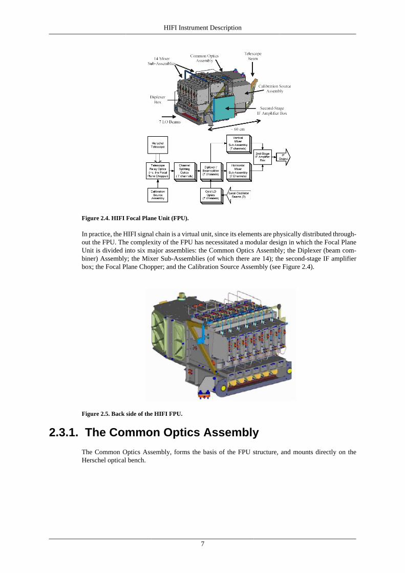
Figure 2.4. HIFI Focal Plane Unit (FPU).
In practice, the HIFI signal chain is a virtual unit, since its elements are physically distributed through-out the FPU. The complexity of the FPU has necessitated a modular design in which the Focal PlaneUnit is divided into six major assemblies: the Common Optics Assembly; the Diplexer (beam com-biner) Assembly; the Mixer Sub-Assemblies (of which there are 14); the second-stage IF amplifierbox; the Focal Plane Chopper; and the Calibration Source Assembly (see Figure 2.4).
Figure 2.5. Back side of the HIFI FPU.
2.3.1. The Common Optics Assembly
The Common Optics Assembly, forms the basis of the FPU structure, and mounts directly on theHerschel optical bench.
HIFI Instrument Description
8
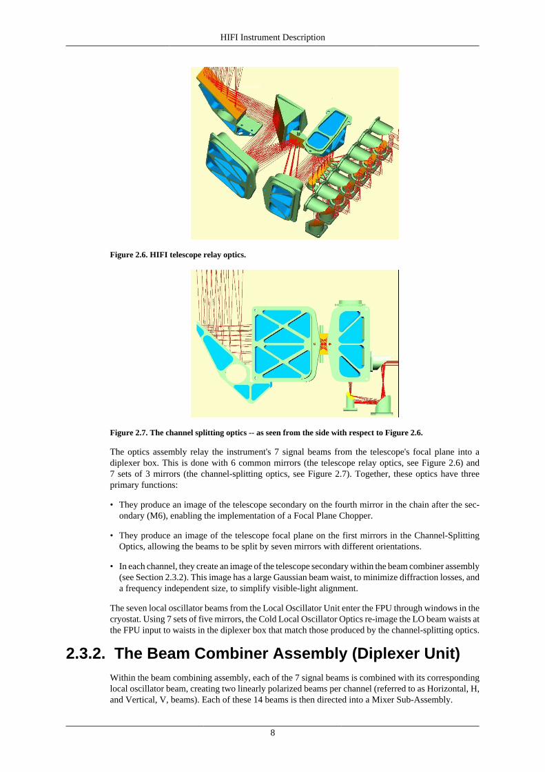
Figure 2.6. HIFI telescope relay optics.
Figure 2.7. The channel splitting optics -- as seen from the side with respect to Figure 2.6.
The optics assembly relay the instrument's 7 signal beams from the telescope's focal plane into adiplexer box. This is done with 6 common mirrors (the telescope relay optics, see Figure 2.6) and7 sets of 3 mirrors (the channel-splitting optics, see Figure 2.7). Together, these optics have threeprimary functions:
• They produce an image of the telescope secondary on the fourth mirror in the chain after the sec-ondary (M6), enabling the implementation of a Focal Plane Chopper.
• They produce an image of the telescope focal plane on the first mirrors in the Channel-SplittingOptics, allowing the beams to be split by seven mirrors with different orientations.
• In each channel, they create an image of the telescope secondary within the beam combiner assembly(see Section 2.3.2). This image has a large Gaussian beam waist, to minimize diffraction losses, anda frequency independent size, to simplify visible-light alignment.
The seven local oscillator beams from the Local Oscillator Unit enter the FPU through windows in thecryostat. Using 7 sets of five mirrors, the Cold Local Oscillator Optics re-image the LO beam waists atthe FPU input to waists in the diplexer box that match those produced by the channel-splitting optics.
2.3.2. The Beam Combiner Assembly (Diplexer Unit)Within the beam combining assembly, each of the 7 signal beams is combined with its correspondinglocal oscillator beam, creating two linearly polarized beams per channel (referred to as Horizontal, H,and Vertical, V, beams). Each of these 14 beams is then directed into a Mixer Sub-Assembly.
HIFI Instrument Description
9
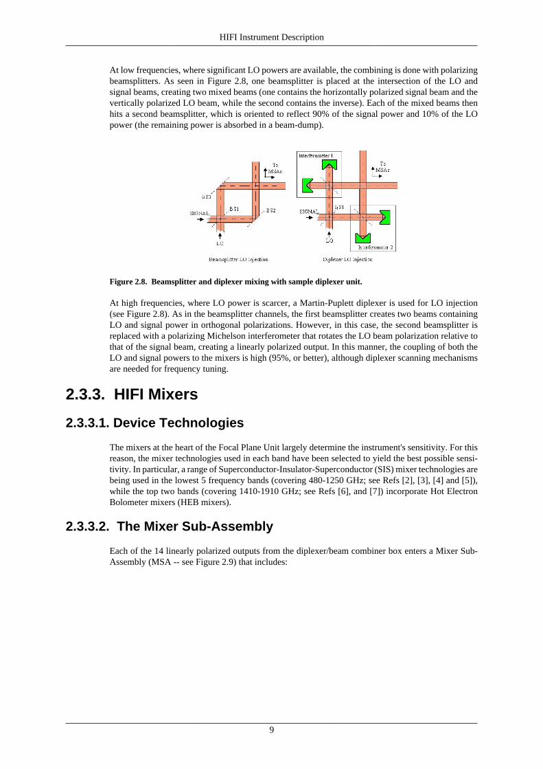
At low frequencies, where significant LO powers are available, the combining is done with polarizingbeamsplitters. As seen in Figure 2.8, one beamsplitter is placed at the intersection of the LO andsignal beams, creating two mixed beams (one contains the horizontally polarized signal beam and thevertically polarized LO beam, while the second contains the inverse). Each of the mixed beams thenhits a second beamsplitter, which is oriented to reflect 90% of the signal power and 10% of the LOpower (the remaining power is absorbed in a beam-dump).
Figure 2.8. Beamsplitter and diplexer mixing with sample diplexer unit.
At high frequencies, where LO power is scarcer, a Martin-Puplett diplexer is used for LO injection(see Figure 2.8). As in the beamsplitter channels, the first beamsplitter creates two beams containingLO and signal power in orthogonal polarizations. However, in this case, the second beamsplitter isreplaced with a polarizing Michelson interferometer that rotates the LO beam polarization relative tothat of the signal beam, creating a linearly polarized output. In this manner, the coupling of both theLO and signal powers to the mixers is high (95%, or better), although diplexer scanning mechanismsare needed for frequency tuning.
2.3.3. HIFI Mixers
2.3.3.1. Device Technologies
The mixers at the heart of the Focal Plane Unit largely determine the instrument's sensitivity. For thisreason, the mixer technologies used in each band have been selected to yield the best possible sensi-tivity. In particular, a range of Superconductor-Insulator-Superconductor (SIS) mixer technologies arebeing used in the lowest 5 frequency bands (covering 480-1250 GHz; see Refs [2], [3], [4] and [5]),while the top two bands (covering 1410-1910 GHz; see Refs [6], and [7]) incorporate Hot ElectronBolometer mixers (HEB mixers).
2.3.3.2. The Mixer Sub-Assembly
Each of the 14 linearly polarized outputs from the diplexer/beam combiner box enters a Mixer Sub-Assembly (MSA -- see Figure 2.9) that includes:
HIFI Instrument Description
10
Figure 2.9. A HIFI mixer sub-assembly.
• a set of three mirrors that focus the optical beam into the mixer;
• a mixer unit where the incoming signal and LO signal are combined;
• a low-noise IF amplifier (plus two IF isolators - for bands 1 to 5 - that suppress reflections in thecable between the mixer and the amplifier);
• low-frequency filtering for the mixers DC bias lines; and
• a mechanical structure that thermally isolates the mixer unit (at 2 K) from the FPU structure (at10 K).
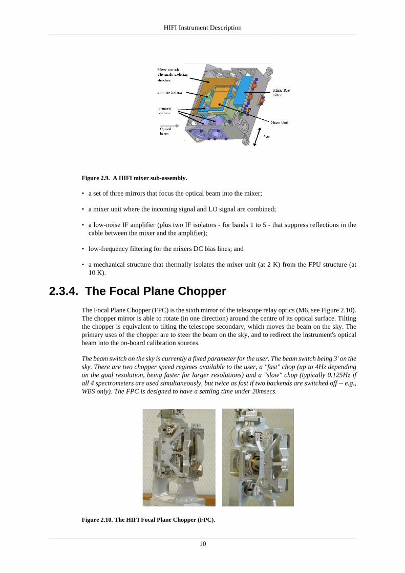
2.3.4. The Focal Plane ChopperThe Focal Plane Chopper (FPC) is the sixth mirror of the telescope relay optics (M6, see Figure 2.10).The chopper mirror is able to rotate (in one direction) around the centre of its optical surface. Tiltingthe chopper is equivalent to tilting the telescope secondary, which moves the beam on the sky. Theprimary uses of the chopper are to steer the beam on the sky, and to redirect the instrument's opticalbeam into the on-board calibration sources.
The beam switch on the sky is currently a fixed parameter for the user. The beam switch being 3' on thesky. There are two chopper speed regimes available to the user, a "fast" chop (up to 4Hz dependingon the goal resolution, being faster for larger resolutions) and a "slow" chop (typically 0.125Hz ifall 4 spectrometers are used simultaneously, but twice as fast if two backends are switched off -- e.g.,WBS only). The FPC is designed to have a settling time under 20msecs.
Figure 2.10. The HIFI Focal Plane Chopper (FPC).
HIFI Instrument Description
11
2.3.5. The Calibration Source AssemblyMounted on the side of the Common Optics Assembly, the Calibration Source Assembly includes twoblackbody signal loads that are used to calibrate the instrument's sensitivity (the first is an absorberat the FPU temperature around 10K, while the second is a lightweight blackbody cavity that can beheated to 100K), plus mirrors that focus the FPU's optical beam into the loads. Temperature sensorsare available to read out the actual temperature of both calibration loads. The HIFI optical beam issteered towards the calibration sources by the use of extreme positions of the Focal Plane Chopper.
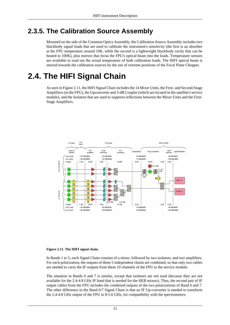
2.4. The HIFI Signal ChainAs seen in Figure 2.11, the HIFI Signal Chain includes the 14 Mixer Units, the First- and Second-StageAmplifiers (in the FPU), the Upconverter and 3-dB Coupler (which are located in the satellite's servicemodule), and the Isolators that are used to suppress reflections between the Mixer Units and the First-Stage Amplifiers.
Figure 2.11. The HIFI signal chain.
In Bands 1 to 5, each Signal Chain consists of a mixer, followed by two isolators, and two amplifiers.For each polarization, the outputs of these 5 independent chains are combined, so that only two cablesare needed to carry the IF outputs from these 10 channels of the FPU to the service module.
The situation in Bands 6 and 7 is similar, except that isolators are not used (because they are notavailable for the 2.4-4.8 GHz IF band that is needed for the HEB mixers). Thus, the second pair of IFoutput cables from the FPU includes the combined outputs of the two polarizations of Band 6 and 7.The other difference in the Band 6/7 Signal Chain is that an IF Up-converter is needed to transformthe 2.4-4.8 GHz output of the FPU to 8-5.6 GHz, for compatibility with the spectrometers.
HIFI Instrument Description
12
Within the "IF Up-converter" (in the service module), a 3-dB Coupler is also used to combine theBands 1-5 and 6-7 outputs, so that each "polarization" of the Wide-Band and High-Resolution Spec-trometers is connected to all 7 bands by a single input cable (although a signal is only received fromthe active band).
2.5. HIFI SpectrometersThe HIFI instrument provides an IF bandwidth of 4GHz in all bands except for band 6 and band 7(1408-1908GHz) where only 2.4GHz bandwidth is available. To sample this bandwidth, HIFI has4 spectrometers. A Wide Band Spectrometer (WBS) and High Resolution Spectrometer (HRS) areavailable for each of the polarizations. All spectrometers can be used in parallel, although at fast datarates it is necessary to reduce how much is readout and stored since, at the highest data rates, thespectrometers provide data at a rate that is higher than the bandwidth available to HIFI on board thespacecraft.
The WBS is an Acousto-Optical Spectrometer (AOS) able to cover the full IF range available (4GHz)at a single resolution (1.1MHz). The HRS is an Auto-Correlator System (ACS) with several possibleresolutions from 0.125 to 1.00MHz but with a variable bandwidth that can cover only portions ofthe available IF range. The HRS can be split up to allow the sampling of more than one part of theavailable IF range.
In the following two subsections, we describe the main workings of the two spectrometer types avail-able to HIFI.
2.5.1. The Wide Band Spectrometer (WBS)The WBS is based on two (vertical and horizontal polarization) four channel Acousto-Optical Spec-trometers (AOS; see [8]) and includes IF processing and data acquisition. To cover the 2 x 4-8 GHz (2x 2.4-4.8GHz for bands 6 and 7) input signals from the FPU, two complete spectrometers (horizontal+ vertical polarization) are used. For redundancy reasons both spectrometers are fully independent.
Each spectrometer receives a pre-amplified and filtered IF-signal (4-8 GHz). After further amplifica-tion in the WBS electronics, the signal is split into four channels which provide the input frequencybands for the WBS optics (4 x 1.55-2.65 GHz; IF1 to IF4). The signal is further amplified and equalised(using variable attenuators), to compensate for non-uniform gain of the system, before being sent totwo Bragg cells in the optics module of the WBS.
The other necessary input is to provide a frequency reference signal for the frequency calibrationof WBS spectra. This is done using a 10 MHz reference signal from the Local Oscillator SourceUnit (LSU), is fed into the WBS to provide a "comb" signal. The comb signal in the WBS, withregular stable 100 MHz line spacing, can be connected for frequency calibration purposes or it canbe disabled to provide a zero level measurement of the AOSs. The zero allows allows more precisesystem temperature measurements to be made.
In the optics section of the WBS, the pre-processed IF-signal from the mixers is analysed using theacousto-optic technique. The IF-signal is fed into a Bragg cell via a transducer. The IF-signal thengenerates an acoustic wave pattern in the Bragg cell crystal. A laser beam which enters the Bragg cellis diffracted according to the acoustic wave pattern in the Bragg cell crystal. The diffracted laser lightis afterwards detected by four linear CCDs with 2048 pixels each and each covering approximately1GHz bandwidth. Four vertically aligned Bragg cells and CCD chains are necessary to cover the full4 GHz IF bandwidth of HIFI.
The WBE electronic section has 4 analogue line receivers for the 4 CCD video signals. These signalsare fed to 14 Bit analogue to digital converter with a conversion speed corresponding to less than 3ms. The relatively high number of ADC-Bit is meant to keep differential non-linearity effects to a verylow level. Overall non-linearity in the WBS is very low, less than 1%..
Continuous data taking is possible without dead time during data transfer, as long as the integrationtime is above 1 sec -- which is true for all standard operating modes of HIFI.
HIFI Instrument Description
13
Every 10 ms the collected photoelectrons in the CCD photodiodes are shifted into a register andclocked out serially. After integration completion, the data can be transferred while a new integrationis started. Data is transmitted to the Instrument Control Unit (ICU) with 16 or 24 Bits through a serialinterface with 250 kHz clock rate which is synchronous with the CCD read-out clock. Housekeepingdata is provided through the same interface. A second serial interface is used for the command inter-face.
2.5.2. The High Resolution Spectrometer (HRS)With the HRS, high resolution spectra are available from any part of the input IF bandwidth (4GHz, or2.4GHz in band 6 or 7). The HRS is an Auto-Correlator Spectrometer (ACS) that can process simulta-neously the 2 signals coming from each polarization of the FPU. It is composed of two identical units:HRS-H and HRS-V. Each of which includes an IF processor, a Digital Autocorrelator Spectrometer(ACS) and associated digital electronics, plus a DC/DC converter (not discussed here). The HRS pro-vides capability to analyse 4 subbands per polarization, placed anywhere in the 2.4 or 4 GHz inputbands coming from the Focal Plane Unit (FPU). The two units of the HRS can be used to processthe same 4 sub-band frequency ranges in each of the two polarizations provided by the FPU, therebyreducing the integration time and providing redundancy. Both units of the HRS operate at the sametime and it is possible to look at either IF with each of the HRS spectrometers.
2.5.2.1. Overview of the HRS Subsystem
In each HRS unit the ACS processes the signals coming from its associated IF (see [9]). Each 230MHz band width input is digitized by a 2 bit / 3 level analogue to digital converter clocked at 490MHz. The digital signals are analysed with a total of 4080 autocorrelation channels. It is possible toconfigure the HRS to provide 4 standard modes of operation as given in Table 3.2. For example, inits nominal resolution the HRS proves two sub-band spectra each of which have a bandwidth of 230MHz, each of which is covered by 2040 channels and has a spectral resolution of 250kHz.
It is possible to set each sub-band frequency independently anywhere in the 4 GHz IF band range.
Two buffers are used, with selection synchronised with the chopper position by the ICU. The HRShas a maximum chopping frequency of 5 Hz. The data can be accumulated in each buffer up to amaximum of 1.95 seconds. The data readout duration is about 42 ms. Data can be read out from onebuffer while data accumulation occurs on the other.
2.5.2.2. Modes of HRS Operation -- Wide Band Mode
In the wide band mode all 4080 correlation channels of the ACS are used to analyse the 8 input signals.As the input signals are adjacent two by two, 4 sub-bands of each of 460 MHz bandwidth can beanalysed in this mode. The four sub-bands can be independently placed anywhere in the IF bandwidthrange. It is possible to analyse almost the whole 4 GHz input IF bandwidth by selecting the samepolarization in the two HRS units and by setting the lose to have adjacent sub-bands.
In this mode, with a Hanning windowing of the correlation function, the spectral resolution is 1000kHz. The total band-width per HRS unit is 2 GHz.
In each correlator ASIC one channel is dedicated to compute the analogue signal offset.
2.5.2.3. Modes of HRS Operation -- Low Resolution Mode
In the low resolution mode the 4080 correlation channels are used to analyse 4 of the 8 input signalsof 230 MHz band width each. The four sub-bands can be independently placed anywhere in the IFbandwidth.
In this mode, with a Hanning windowing of the correlation function, the spectral resolution is 500kHz. The total band-width per HRS unit is 1 GHz.
In each correlator ASIC one channel is dedicated to compute the analogue signal offset.
HIFI Instrument Description
14
2.5.2.4. Modes of HRS Operation -- Nominal Resolution Mode
In the nominal resolution mode the 4080 correlation channels are used to analyse 2 of the 8 inputsignals of 230 MHz band width each. The two sub-bands can be independently placed anywhere inthe IF bandwidth range.
In this mode, with a Hanning windowing of the correlation function, the spectral resolution is 250kHz. The total band-width per HRS unit is 460 MHz.
In each correlator ASIC one channel is dedicated to compute the analogue signal offset.
2.5.2.5. Modes of HRS Operation -- High Resolution Mode
In the high resolution mode the 4080 correlation channels are used to analyse 1 of the 8 input signalsof 230 MHz band width each. The sub-band can be placed anywhere in the IF bandwidth range.
In this mode, with a Hanning windowing of the correlation function, the spectral resolution is 125kHz. The total band-width per HRS unit is 230 MHz.
In each correlator ASIC one channel is dedicated to compute the analogue signal offset.
15
Chapter 3. HIFI Scientific Capabilitiesand Performance
The HIFI instrument has been designed to provide very high spectral resolution across a large rangeof far-infrared and sub-millimetre wavelengths. A large fraction of the frequency range covered bythe instrument can not be observed from the ground.
In this chapter we discuss the range of science capabilities of the instrument.
3.1. What Science Is Possible With HIFI?HIFI's very high spectral resolution coupled with its ability to observe thousands of molecular, atomicand ionic lines at sub-millimeter wavelengths make it the instrument of choice to address many ofthe key questions in modern astrophysics related to the cyclic interaction of stars and the interstellarmedium. A wide range of chemical and dynamical studies are possible using HIFI. However, theoriginal set of science objectives for the instrument are given in the following section.
3.1.1. HIFI's Scientific Objectives
At the outset of the mission, the major scientific objectives of the HIFI instrument are:
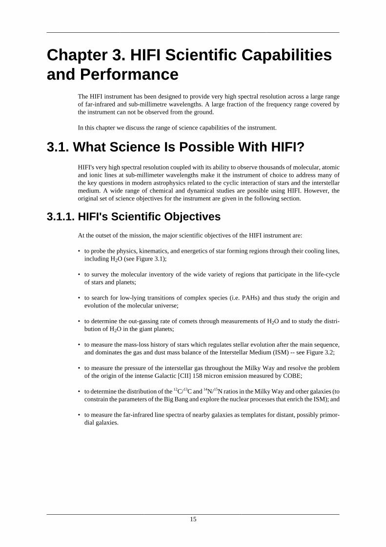
• to probe the physics, kinematics, and energetics of star forming regions through their cooling lines,including H2O (see Figure 3.1);
• to survey the molecular inventory of the wide variety of regions that participate in the life-cycleof stars and planets;
• to search for low-lying transitions of complex species (i.e. PAHs) and thus study the origin andevolution of the molecular universe;
• to determine the out-gassing rate of comets through measurements of H2O and to study the distri-bution of H2O in the giant planets;
• to measure the mass-loss history of stars which regulates stellar evolution after the main sequence,and dominates the gas and dust mass balance of the Interstellar Medium (ISM) -- see Figure 3.2;
• to measure the pressure of the interstellar gas throughout the Milky Way and resolve the problemof the origin of the intense Galactic [CII] 158 micron emission measured by COBE;
• to determine the distribution of the 12C/13C and 14N/15N ratios in the Milky Way and other galaxies (toconstrain the parameters of the Big Bang and explore the nuclear processes that enrich the ISM); and
• to measure the far-infrared line spectra of nearby galaxies as templates for distant, possibly primor-dial galaxies.
HIFI Scientific Capabilities and Performance
16
Figure 3.1. One of HIFI's first spectra. The 557 GHz water line as seen in Comet Garradd
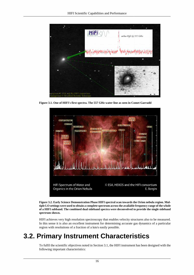
Figure 3.2. Early Science Demonstration Phase HIFI spectral scan towards the Orion nebula region. Mul-tiple LO settings were used to obtain a complete spectrum across the available frequency range of the wholeof a HIFI subband. The combined dual sideband spectra were deconvolved to provide the single sidebandspectrum shown.
HIFI achieves very high resolution spectroscopy that enables velocity structures also to be measured.In this sense it is also an excellent instrument for determining accurate gas dynamics of a particularregion with resolutions of a fraction of a km/s easily possible.
3.2. Primary Instrument CharacteristicsTo fulfil the scientific objectives noted in Section 3.1, the HIFI instrument has been designed with thefollowing important characteristics:
HIFI Scientific Capabilities and Performance
17
• complete coverage of 480-1250 and 1410-1910 GHz (625-240 and 213-157 microns), to allowmultiples lines of important molecules, such as H2O, to be sampled, and to allow broad, unbiasedspectral surveys;
• a resolving power of up to 107, corresponding to a velocity resolution up to 0.03 km/s (requiringa narrow local oscillator line-width and an Intermediate Frequency (IF) spectrometer -- measuringthe frequency difference between signal and local oscillator signals -- with a resolution of up to125 kHz);
• a receiver sensitivity of 3-4 times the quantum limit, to make maximum use of the limited satellitelifetime (requiring low-noise mixers and IF amplifiers);
• a large instantaneous band-width (4 GHz in each sideband) to increase spectral survey speeds, tominimize the risk of spectral coverage gaps, and to observe broad features (requiring mixers, am-plifiers, and a spectrometer with 4 GHz of IF bandwidth);
• dual-polarization operation to make maximum use of the energy collected by the HIFI optical beam;and
• at least 10% calibration accuracy (with a goal of 3%)
NOTES:
1. The time needed to observe a weak spectral line scales inversely with the square of the receivernoise temperature.
2. The bandwidth is only 2.4 GHz in Bands 6 and 7 (due to a bandwidth limitation in the state-of-the-art HEB mixers that are used at these high frequencies).
3. For bands 5, 6 and 7, the receiver temperatures are rather 10-20 times the quantum limit.
3.3. General Instrument DescriptionThe HIFI instrument provides continuous frequency coverage over the range 480-1250 GHz (625-240microns) in five bands with approximately equal tuning range. An additional pair of bands providecoverage of the frequency range 1410-1910 GHz (213-157 microns). The instrument operates at onlyone local oscillator frequency at a time.
In all mixer bands two independent mixers receive both horizontal and vertical polarizations of theastronomical signal, although in some cases reduced bandwidth or use of a single polarization is re-quired to stay within the data rate available to the instrument.
The user has the choice of using only a single polarization if he/she chooses.
The first 5 mixer bands use SIS (superconductor-insulator-superconductor) mixers; bands 6 and 7, useHot-Electron Bolometers (HEBs).
The instantaneous bandwidth of the instrument will be 4 GHz. The frequency coverage of the instru-ment is summarised in Table 3.1.
HIFI Scientific Capabilities and Performance
18
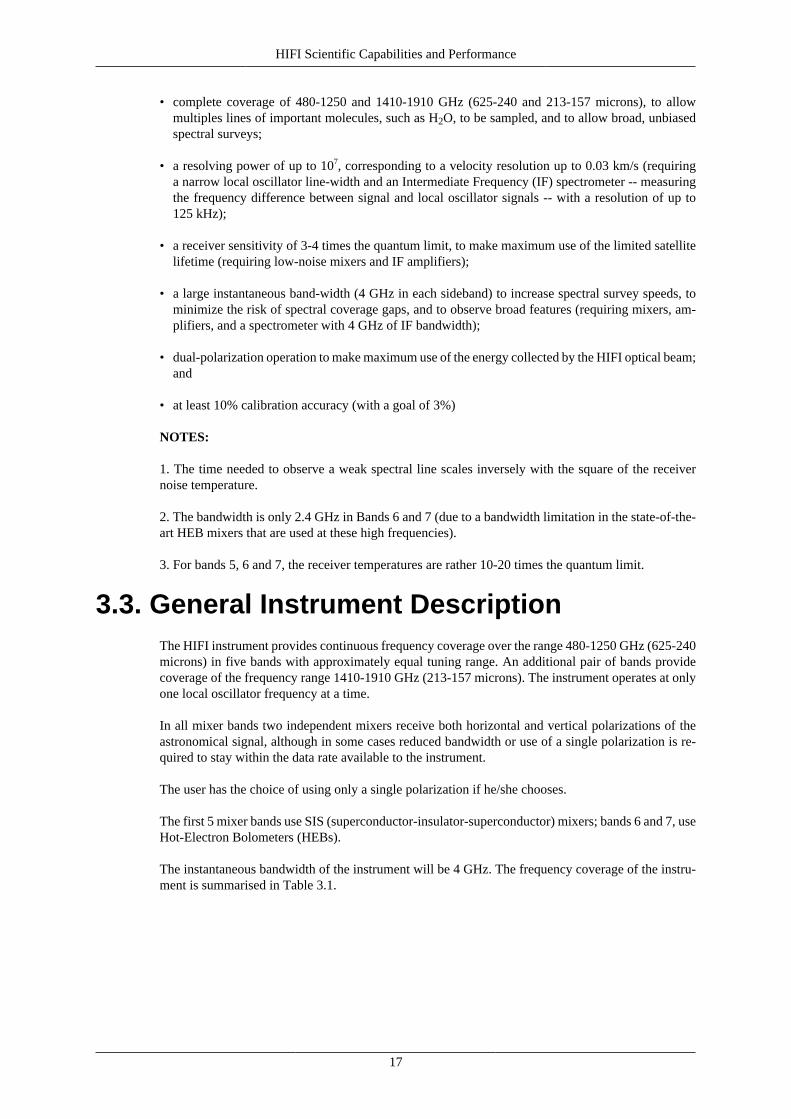
Table 3.1. HIFI frequency coverage and band allocation. Note that the values presented are Local Oscillatorfrequencies. Each band is further split in two ("a" and "b") due to the use of two Local Oscillator chainsfor the lower and upper portions of the frequency range for each band. A further 8GHz is available at eachend of the frequency range due to the frequency placement of the upper and lower sidebands in HIFI inbands 1 to 5. This is only a further 4.8GHz in bands 6 and 7.
Band Mixer typeLO Lowerfreq.
LO Upperfreq.
Beam Size(HPBW)
IF Bandwidth
1 SIS 488.1 GHz 628.4 GHz 39" 4.0 GHz
2 SIS 642.1 GHz 793.9 GHz 30" 4.0 GHz
3 SIS 807.1 GHz 952.9 GHz 25" 4.0 GHz
4 SIS 957.2 GHz 1113.8 GHz 21" 4.0 GHz
5 SIS 1116.2 GHz 1271.8 GHz 19" 4.0 GHz
6 + 7 HEB 1430.2 GHz 1901.8 GHz 13" 2.4 GHz
3.4. Available Spectrometer SetupsHIFI has four spectrometers, one Wide Band Spectrometer (WBS) and one High Resolution Spec-trometer (HRS) per polarization. These may all be used simultaneously. When all spectrometers arein use frame times are 4 seconds each. Shorter frame times are possible when only one type of spec-trometer is used (1 or 2 seconds).
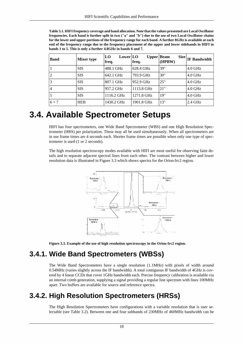
The high resolution spectroscopy modes available with HIFI are most useful for observing faint de-tails and to separate adjacent spectral lines from each other. The contrast between higher and lowerresolution data is illustrated in Figure 3.3 which shows spectra for the Orion-Irc2 region.
Figure 3.3. Example of the use of high resolution spectroscopy in the Orion-Irc2 region.
3.4.1. Wide Band Spectrometers (WBSs)The Wide Band Spectrometers have a single resolution (1.1MHz) with pixels of width around0.54MHz (varies slightly across the IF bandwidth). A total contiguous IF bandwidth of 4GHz is cov-ered by 4 linear CCDs that cover 1GHz bandwidth each. Precise frequency calibration is available viaan internal comb generation, supplying a signal providing a regular line spectrum with lines 100MHzapart. Two buffers are available for source and reference spectra.
3.4.2. High Resolution Spectrometers (HRSs)The High Resolution Spectrometers have configurations with a variable resolution that is user se-lectable (see Table 3.2). Between one and four subbands of 230MHz of 460MHz bandwidth can be
HIFI Scientific Capabilities and Performance
19
centred anywhere within the 4GHz intermediate frequency range made available to the spectrometers.Frequency calibration comes from the internal local oscillator frequency settings for the spectrometer.Two buffers are available for source and reference spectra.
Table 3.2. List of HRS configurations available in each polarization
Mode
Number ofbands per po-larization xbandwidth
Number oflags
Number of off-set channels
Spectral reso-lution (kHz) -Hanning typeapodisation-.
Channel spac-ing (kHz)
High resolution 1 x 230MHz 1 x 4080 16 125 64
Nominal reso-lution
2 x 230MHz 2 x 2040 16 250 125
Low resolution 4 x 230MHz 4 x 10²⁰ 16 500 250
Wide resolu-tion (band)
4 x 460MHz(x2)
4 x 510 (x2) 16 1000 500
3.5. Mixer PerformanceFurther information beyond what is provided here can be found on the Herschel Science Center's web-site for the AO release http://herschel.esac.esa.int/AOTsReleaseStatus.shtml. Please see this area formore detailed information and any updates on HIFI instrument performance and AOTs. The calibra-tion pages will contain up to date calibration information including system temperature vs IF for alltuned LO frequencies (also see Section 3.5.2).
3.5.1. System Temperatures
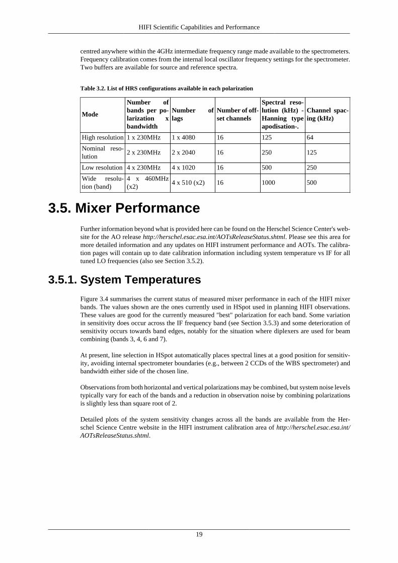
Figure 3.4 summarises the current status of measured mixer performance in each of the HIFI mixerbands. The values shown are the ones currently used in HSpot used in planning HIFI observations.These values are good for the currently measured "best" polarization for each band. Some variationin sensitivity does occur across the IF frequency band (see Section 3.5.3) and some deterioration ofsensitivity occurs towards band edges, notably for the situation where diplexers are used for beamcombining (bands 3, 4, 6 and 7).
At present, line selection in HSpot automatically places spectral lines at a good position for sensitiv-ity, avoiding internal spectrometer boundaries (e.g., between 2 CCDs of the WBS spectrometer) andbandwidth either side of the chosen line.
Observations from both horizontal and vertical polarizations may be combined, but system noise levelstypically vary for each of the bands and a reduction in observation noise by combining polarizationsis slightly less than square root of 2.
Detailed plots of the system sensitivity changes across all the bands are available from the Her-schel Science Centre website in the HIFI instrument calibration area of http://herschel.esac.esa.int/AOTsReleaseStatus.shtml.
HIFI Scientific Capabilities and Performance
20
Figure 3.4. Double sideband system system temperatures of HIFI mixers (bands 1 to 5 are SIS mixers, bands6 and 7 are HEB mixers), as used in HSpot. System temperatures are based on in-flight measurementsusing the internal calibrators of HIFI together with the H and V polarizations of the WBS spectrometer.The institutions that created the different mixer subbands are indicated.
3.5.2. Tuning RangesIn addition to certain known impure frequencies (see Section 5.4.6), the various HIFI LO chains havefrequency ranges in which they cannot provide enough output power in order to sufficiently pump themixers. The receiver noise temperature is very high in these ranges. Unlike the purity issues, however,there is little improvement to be expected on the short term so these areas must be considered asregions of low performance, over the spectral coverage currently achievable by HIFI.
While the border between sensitive and non-sensitive ranges is not abrupt and the noise degradationis often gradual, the band edges are defined and set in HSpot to avoid frequencies where the mixersare not even marginally pumped. Between the formal (HSpot) band limits, Users are able to recognizeLO frequencies which offer lower performances from the output of time estimation in HSpot: at therequested LO frequency (Point and Map AOTs), the noise temperature is quoted in the Message win-dow. The effect of higher noise temperature is to increase the observing time at a fixed noise goal(entered by the User), or conversely to reduce the S/N ratio at a fixed observing time goal. It is alwaysworthwhile for the User to attempt to find a setting which minimizes the noise, where some flexibilityis allowed in the IF placement of the spectral line(s) of interest.
Note that system temperatures have been measured to a granularity of ~2 GHz, and therefore onlysignificant differences may be noticed when changing the LO frequency that switches the target line(s)from one image band to the other.
Figure 3.4 illustrates the overall distribution of the receiver noise temperatures as measured in flight.All temperatures are the median DSB receiver temperatures over the full WBS bandwidth, in K. Fre-quencies are in GHz. There are two types of poor sensitivity ranges:
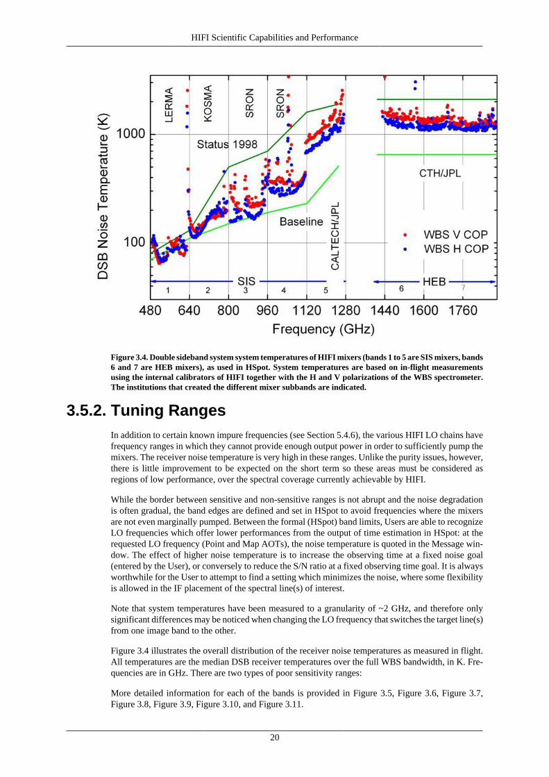
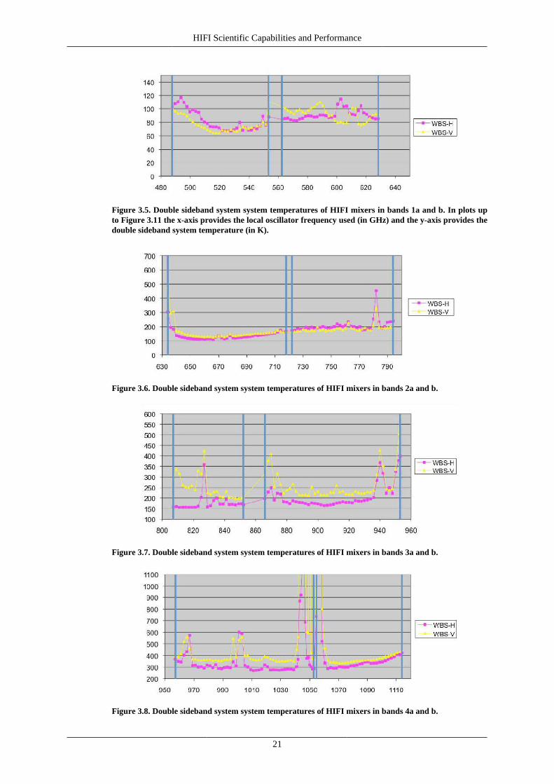
More detailed information for each of the bands is provided in Figure 3.5, Figure 3.6, Figure 3.7,Figure 3.8, Figure 3.9, Figure 3.10, and Figure 3.11.
HIFI Scientific Capabilities and Performance
21
Figure 3.5. Double sideband system system temperatures of HIFI mixers in bands 1a and b. In plots upto Figure 3.11 the x-axis provides the local oscillator frequency used (in GHz) and the y-axis provides thedouble sideband system temperature (in K).
Figure 3.6. Double sideband system system temperatures of HIFI mixers in bands 2a and b.
Figure 3.7. Double sideband system system temperatures of HIFI mixers in bands 3a and b.
Figure 3.8. Double sideband system system temperatures of HIFI mixers in bands 4a and b.
HIFI Scientific Capabilities and Performance
22
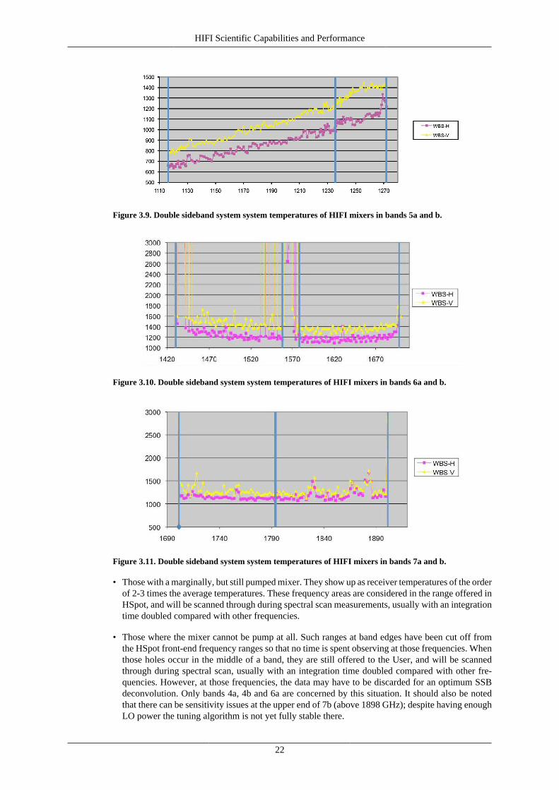
Figure 3.9. Double sideband system system temperatures of HIFI mixers in bands 5a and b.
Figure 3.10. Double sideband system system temperatures of HIFI mixers in bands 6a and b.
Figure 3.11. Double sideband system system temperatures of HIFI mixers in bands 7a and b.
• Those with a marginally, but still pumped mixer. They show up as receiver temperatures of the orderof 2-3 times the average temperatures. These frequency areas are considered in the range offered inHSpot, and will be scanned through during spectral scan measurements, usually with an integrationtime doubled compared with other frequencies.
• Those where the mixer cannot be pump at all. Such ranges at band edges have been cut off fromthe HSpot front-end frequency ranges so that no time is spent observing at those frequencies. Whenthose holes occur in the middle of a band, they are still offered to the User, and will be scannedthrough during spectral scan, usually with an integration time doubled compared with other fre-quencies. However, at those frequencies, the data may have to be discarded for an optimum SSBdeconvolution. Only bands 4a, 4b and 6a are concerned by this situation. It should also be notedthat there can be sensitivity issues at the upper end of 7b (above 1898 GHz); despite having enoughLO power the tuning algorithm is not yet fully stable there.
HIFI Scientific Capabilities and Performance
23
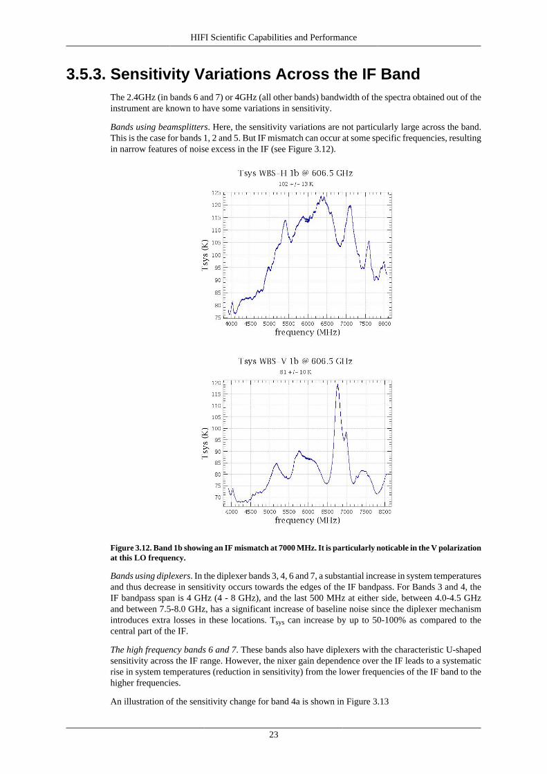
3.5.3. Sensitivity Variations Across the IF BandThe 2.4GHz (in bands 6 and 7) or 4GHz (all other bands) bandwidth of the spectra obtained out of theinstrument are known to have some variations in sensitivity.
Bands using beamsplitters. Here, the sensitivity variations are not particularly large across the band.This is the case for bands 1, 2 and 5. But IF mismatch can occur at some specific frequencies, resultingin narrow features of noise excess in the IF (see Figure 3.12).
Figure 3.12. Band 1b showing an IF mismatch at 7000 MHz. It is particularly noticable in the V polarizationat this LO frequency.
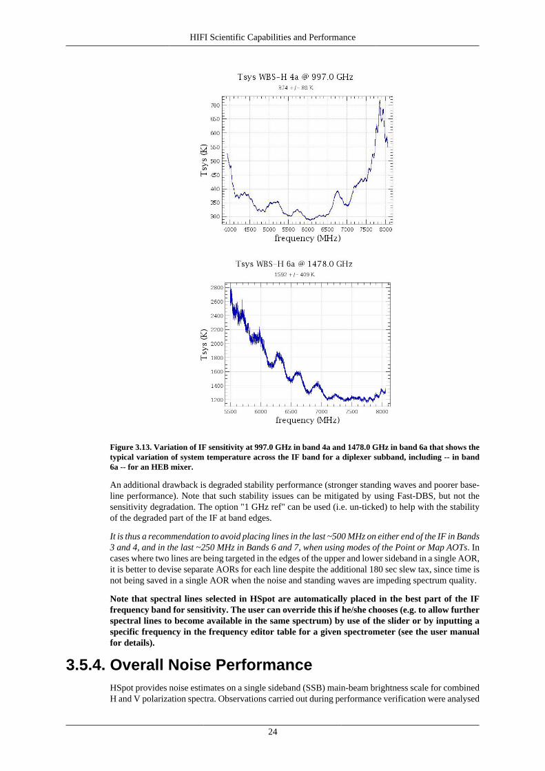
Bands using diplexers. In the diplexer bands 3, 4, 6 and 7, a substantial increase in system temperaturesand thus decrease in sensitivity occurs towards the edges of the IF bandpass. For Bands 3 and 4, theIF bandpass span is 4 GHz (4 - 8 GHz), and the last 500 MHz at either side, between 4.0-4.5 GHzand between 7.5-8.0 GHz, has a significant increase of baseline noise since the diplexer mechanismintroduces extra losses in these locations. Tsys can increase by up to 50-100% as compared to thecentral part of the IF.
The high frequency bands 6 and 7. These bands also have diplexers with the characteristic U-shapedsensitivity across the IF range. However, the nixer gain dependence over the IF leads to a systematicrise in system temperatures (reduction in sensitivity) from the lower frequencies of the IF band to thehigher frequencies.
An illustration of the sensitivity change for band 4a is shown in Figure 3.13
HIFI Scientific Capabilities and Performance
24
Figure 3.13. Variation of IF sensitivity at 997.0 GHz in band 4a and 1478.0 GHz in band 6a that shows thetypical variation of system temperature across the IF band for a diplexer subband, including -- in band6a -- for an HEB mixer.
An additional drawback is degraded stability performance (stronger standing waves and poorer base-line performance). Note that such stability issues can be mitigated by using Fast-DBS, but not thesensitivity degradation. The option "1 GHz ref" can be used (i.e. un-ticked) to help with the stabilityof the degraded part of the IF at band edges.
It is thus a recommendation to avoid placing lines in the last ~500 MHz on either end of the IF in Bands3 and 4, and in the last ~250 MHz in Bands 6 and 7, when using modes of the Point or Map AOTs. Incases where two lines are being targeted in the edges of the upper and lower sideband in a single AOR,it is better to devise separate AORs for each line despite the additional 180 sec slew tax, since time isnot being saved in a single AOR when the noise and standing waves are impeding spectrum quality.
Note that spectral lines selected in HSpot are automatically placed in the best part of the IFfrequency band for sensitivity. The user can override this if he/she chooses (e.g. to allow furtherspectral lines to become available in the same spectrum) by use of the slider or by inputting aspecific frequency in the frequency editor table for a given spectrometer (see the user manualfor details).
3.5.4. Overall Noise PerformanceHSpot provides noise estimates on a single sideband (SSB) main-beam brightness scale for combinedH and V polarization spectra. Observations carried out during performance verification were analysed
HIFI Scientific Capabilities and Performance
25
in order to verify these predictions, which drive observing time at goal and maximum spectral reso-lutions entered in HSpot by the User. The 1 GHz reference option has almost always been used inthe noise predictions, which means that the baseline in only one WBS sub-band is considered for sta-bility instead of the full IF, to take standing waves within that 1 GHz window into account. This isrecommended for most observing situations except, when lines are very broad (such as from externalgalaxies or fast outflows).
Noise estimates from HSpot 5.0 have been found to be consistent with those actually observed usingthe various HIFI observing modes.
3.5.4.1. Noise Performance in Spectral Scans
The noise in the Spectral Scans when measured before sideband deconvolution scales with [2 x redun-dancy]-1/2, to the single sideband (SSB) noise when the gains are equal (0.5). When the gains deviatefrom this value, the deconvolution algorithm should model these as well and the same scaling shouldapply. So far there are no indications of a departure away from 0.5.
Analysis of the Spectral Scans taken during performance verification indicate that the deconvolvedSSB root mean square (RMS) noise values are found to be in good agreement, but also sometimes1.5 to 2 times higher than the HSpot predictions in Bands 1-5. Very preliminary deconvolution resultsindicate that the HEB Bands 6 & 7 suggest an even higher SSB RMS noise - between 2-3 times morethan currently predicted by HSpot. Further work is ongoing and updates will be provided to users asresults are obtained.
Observers should keep in mind that the production of good SSB spectra is highly dependent on theremoval all artefacts: standing waves, spurs, and the removal of all continuum baselines (linear or non-linear) prior to performing the deconvolution reduction step.
Note: When using the DBS reference mode of the spectral scan in bands 6 and 7 users should use thefast DBS mode rather than normal (slow) chop speed mode.
3.5.5. Mixer Stabilities
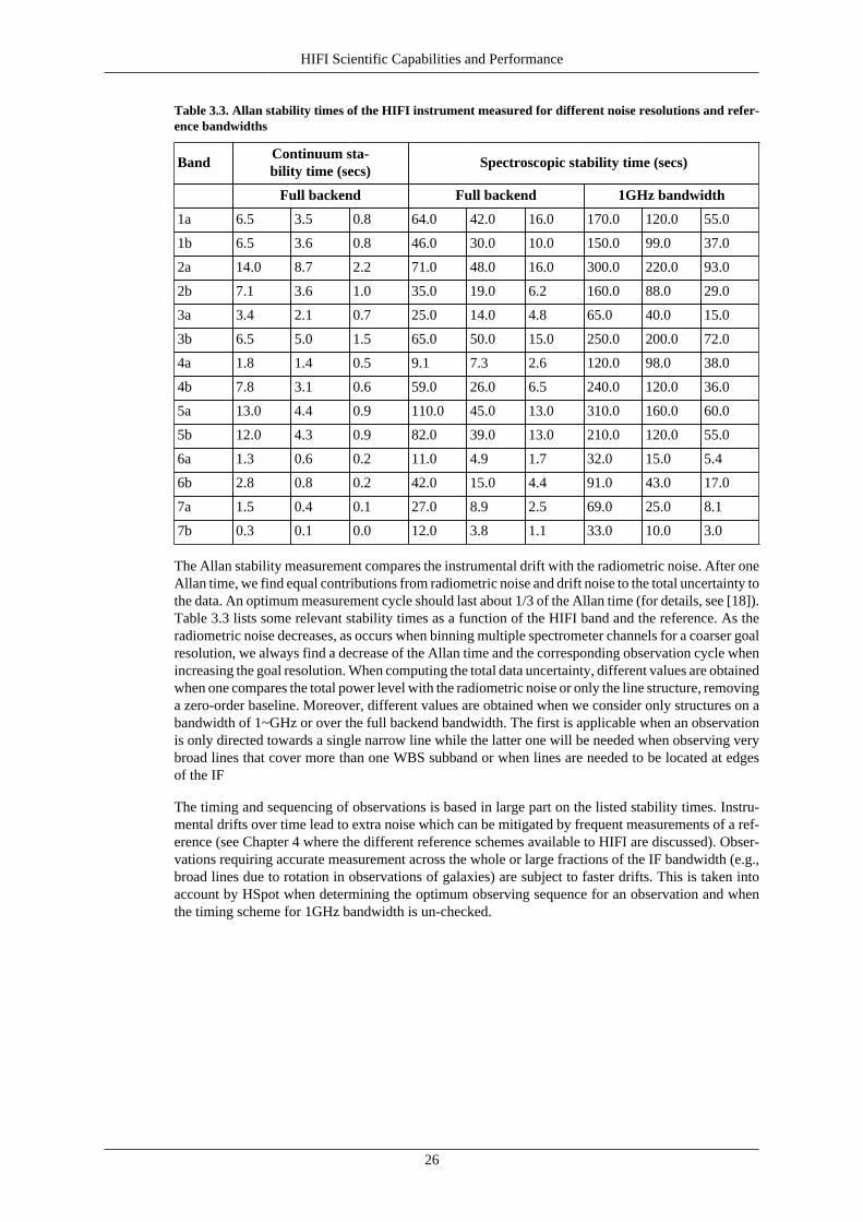
Stability measurements have been made at several frequencies for each of the subbands in flight.Results are now incorporated into the observing sequences produced by HSpot (see Table 3.3).
HIFI Scientific Capabilities and Performance
26
Table 3.3. Allan stability times of the HIFI instrument measured for different noise resolutions and refer-ence bandwidths
BandContinuum sta-bility time (secs)
Spectroscopic stability time (secs)
Full backend Full backend 1GHz bandwidth
1a 6.5 3.5 0.8 64.0 42.0 16.0 170.0 120.0 55.0
1b 6.5 3.6 0.8 46.0 30.0 10.0 150.0 99.0 37.0
2a 14.0 8.7 2.2 71.0 48.0 16.0 300.0 220.0 93.0
2b 7.1 3.6 1.0 35.0 19.0 6.2 160.0 88.0 29.0
3a 3.4 2.1 0.7 25.0 14.0 4.8 65.0 40.0 15.0
3b 6.5 5.0 1.5 65.0 50.0 15.0 250.0 200.0 72.0
4a 1.8 1.4 0.5 9.1 7.3 2.6 120.0 98.0 38.0
4b 7.8 3.1 0.6 59.0 26.0 6.5 240.0 120.0 36.0
5a 13.0 4.4 0.9 110.0 45.0 13.0 310.0 160.0 60.0
5b 12.0 4.3 0.9 82.0 39.0 13.0 210.0 120.0 55.0
6a 1.3 0.6 0.2 11.0 4.9 1.7 32.0 15.0 5.4
6b 2.8 0.8 0.2 42.0 15.0 4.4 91.0 43.0 17.0
7a 1.5 0.4 0.1 27.0 8.9 2.5 69.0 25.0 8.1
7b 0.3 0.1 0.0 12.0 3.8 1.1 33.0 10.0 3.0
The Allan stability measurement compares the instrumental drift with the radiometric noise. After oneAllan time, we find equal contributions from radiometric noise and drift noise to the total uncertainty tothe data. An optimum measurement cycle should last about 1/3 of the Allan time (for details, see [18]).Table 3.3 lists some relevant stability times as a function of the HIFI band and the reference. As theradiometric noise decreases, as occurs when binning multiple spectrometer channels for a coarser goalresolution, we always find a decrease of the Allan time and the corresponding observation cycle whenincreasing the goal resolution. When computing the total data uncertainty, different values are obtainedwhen one compares the total power level with the radiometric noise or only the line structure, removinga zero-order baseline. Moreover, different values are obtained when we consider only structures on abandwidth of 1~GHz or over the full backend bandwidth. The first is applicable when an observationis only directed towards a single narrow line while the latter one will be needed when observing verybroad lines that cover more than one WBS subband or when lines are needed to be located at edgesof the IF
The timing and sequencing of observations is based in large part on the listed stability times. Instru-mental drifts over time lead to extra noise which can be mitigated by frequent measurements of a ref-erence (see Chapter 4 where the different reference schemes available to HIFI are discussed). Obser-vations requiring accurate measurement across the whole or large fractions of the IF bandwidth (e.g.,broad lines due to rotation in observations of galaxies) are subject to faster drifts. This is taken intoaccount by HSpot when determining the optimum observing sequence for an observation and whenthe timing scheme for 1GHz bandwidth is un-checked.
27
Chapter 4. Observing with HIFI
4.1. IntroductionFor HIFI, three Astronomical Observing Templates (AOTs) are available:
• AOT I: Single Point, for observing science targets at one position on the sky;
• AOT II: Mapping, for covering extended regions;
• AOT III: Spectral Scanning, for surveying a single position on the sky over a continuous rangeof frequencies selected within the same LO band by the user.
Each AOT can be used in a variety of different modes of operation, providing the widest range ofoptions for performing spectroscopic science observations in different astronomical that HIFI andthe Observatory will allow, in terms of reference measurements and calibration. In other words, thethree AOTs come with Observing Modes where the user may select from different calibration modes,choosing the mode best suited to the observing situation and science goals.
The Observing Modes are available to the user through the HSpot observation planning tool availablein the Herschel Proposal Handling System.
The Observing Modes are described in the following sections, with typical usage examples and limi-tations, and steps for creating Astronomical Observing Requests (AORs) in HSpot, which representreal observations.
Regardless of mode, however, users of HIFI should be aware of the following general condition:
• Only one LO band is planned to be operated at any one time, meaning that observationsrequiring frequencies in different LO bands will always require separate AORs. AORs makinguse of the same LO band can be scheduled together (e.g., via chaining), but the same schedulingrestrictions that apply to different instruments will also apply to AORs requiring differing LO bands.For instance, it is currently not be possible to group or concatenate different instruments or, in HIFI'scase, different LO bands together, under most circumstances.
• Source integration times will be optimised according to the user's observing time goal or noise levelgoal. Providing user input is discussed in Chapter 6, where specific examples for setting up HIFIobservations are given using the HSpot tool.
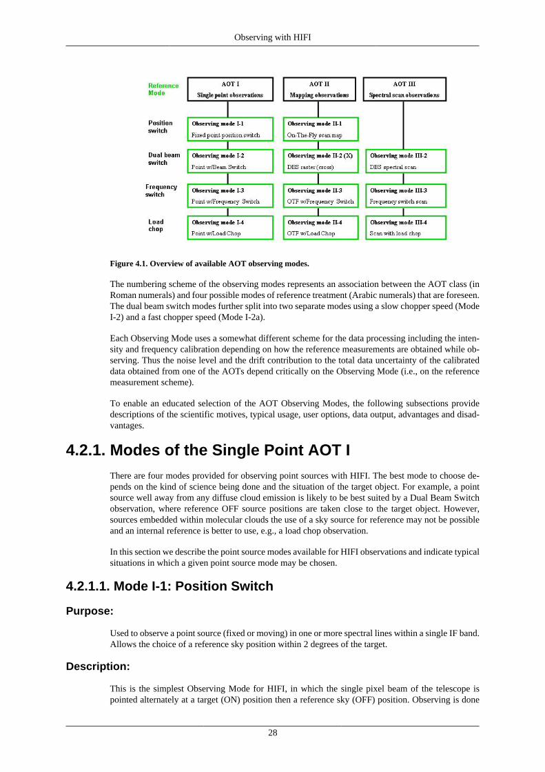
4.2. The HIFI Observing ModesObservations created in one of the three AOTs will be performed in a number of different ObservingModes, which differ mainly in the selection of the reference measurements during the course of ob-serving. All observations consist of source measurements, reference measurements and a set of cali-bration measurements that will be used to fully calibrate the spectra in both frequency and intensity.Observing mode design is intended to supply an optimum balance between observing efficiency andself-contained calibrations timed by instrumental performance and stability metrics. The currently de-signed Observing Modes and their relation to the AOTs is given in the following chart (Figure 4.1):
Observing with HIFI
28
Figure 4.1. Overview of available AOT observing modes.
The numbering scheme of the observing modes represents an association between the AOT class (inRoman numerals) and four possible modes of reference treatment (Arabic numerals) that are foreseen.The dual beam switch modes further split into two separate modes using a slow chopper speed (ModeI-2) and a fast chopper speed (Mode I-2a).
Each Observing Mode uses a somewhat different scheme for the data processing including the inten-sity and frequency calibration depending on how the reference measurements are obtained while ob-serving. Thus the noise level and the drift contribution to the total data uncertainty of the calibrateddata obtained from one of the AOTs depend critically on the Observing Mode (i.e., on the referencemeasurement scheme).
To enable an educated selection of the AOT Observing Modes, the following subsections providedescriptions of the scientific motives, typical usage, user options, data output, advantages and disad-vantages.
4.2.1. Modes of the Single Point AOT IThere are four modes provided for observing point sources with HIFI. The best mode to choose de-pends on the kind of science being done and the situation of the target object. For example, a pointsource well away from any diffuse cloud emission is likely to be best suited by a Dual Beam Switchobservation, where reference OFF source positions are taken close to the target object. However,sources embedded within molecular clouds the use of a sky source for reference may not be possibleand an internal reference is better to use, e.g., a load chop observation.
In this section we describe the point source modes available for HIFI observations and indicate typicalsituations in which a given point source mode may be chosen.
4.2.1.1. Mode I-1: Position Switch
Purpose:
Used to observe a point source (fixed or moving) in one or more spectral lines within a single IF band.Allows the choice of a reference sky position within 2 degrees of the target.
Description:
This is the simplest Observing Mode for HIFI, in which the single pixel beam of the telescope ispointed alternately at a target (ON) position then a reference sky (OFF) position. Observing is done
Observing with HIFI
29
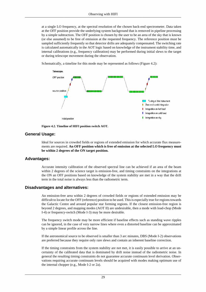
at a single LO frequency, at the spectral resolution of the chosen back-end spectrometer. Data takenat the OFF position provide the underlying system background that is removed in pipeline processingby a simple subtraction. The OFF position is chosen by the user to be an area of the sky that is known(or else assumed) to be free of emission at the requested frequency. The reference position must besampled sufficiently frequently so that detector drifts are adequately compensated. The switching rateis calculated automatically in the AOT logic based on knowledge of the instrument stability time, andinternal calibrations (e.g., frequency calibration) may be performed during initial slews to the targetor during telescope movement during the observation.
Schematically, a timeline for this mode may be represented as follows (Figure 4.2):
Figure 4.2. Timeline of HIFI position switch AOT.
General Usage:
Ideal for sources in crowded fields or regions of extended emission for which accurate flux measure-ments are required. An OFF position which is free of emission at the selected LO frequency mustbe within 2 degrees of the ON target position.
Advantages:
Accurate intensity calibration of the observed spectral line can be achieved if an area of the beamwithin 2 degrees of the science target is emission-free, and timing constraints on the integrations atthe ON an OFF positions based on knowledge of the system stability are met in a way that the driftterm in the total noise is always less than the radiometric term.
Disadvantages and alternatives:
An emission-free area within 2 degrees of crowded fields or regions of extended emission may bedifficult to locate for the OFF (reference) position to be used. This is especially true for regions towardsthe Galactic Centre and around popular star forming regions. If the closest emission-free region isbeyond 2 degrees, and mapping modes (AOT II) are undesirable, then a mode with load-chop (ModeI-4) or frequency-switch (Mode I-3) may be more desirable.
The frequency switch mode may be more efficient if baseline effects such as standing wave ripplescan be ignored, in the case of very narrow lines where even a distorted baseline can be approximatedby a simple linear profile across the line.
If the astronomical source to be observed is smaller than 3 arc minutes, DBS (Mode I-2) observationsare preferred because they require only rare slews and contain an inherent baseline correction.
If the timing constraints from the system stability are not met, it is easily possible to arrive at an un-certainty of the calibrated data that is dominated by drift noise instead of the radiometric noise. Ingeneral the resulting timing constraints do not guarantee accurate continuum level derivation. Obser-vations requiring accurate continuum levels should be acquired with modes making optimum use ofthe internal chopper (e.g., Mode I-2 or 2a).
Observing with HIFI
30
User Inputs:
Target (ON) and reference (OFF) positions, LO band and frequency, minimum and maximum goalfrequency resolution of the calibrated data, spectrometer usage, and total observing time or noise goalat the lowest goal at the goal resolution.
Data Calibration:
The final spectra are based on the differences between neighbouring ON target and OFF referenceposition measurements. Co-addition of (ON - OFF) provide the final 1D spectrum.
A zeroth order baseline may occassionally need to be subtracted when using this mode.
No explicit standing wave correction is needed.
Instrument tuning, frequency calibration, and measurements of the internal hot and cold loads will bedone during initial slew, and may be done during slews between ON and OFF positions dependingon slew length and rate.
The transformation into a brightness temperature scale is performed by dividing the difference mea-surement by the results from the load calibration measurements and multiplying by the correspondingdifference in the Rayleigh-Jeans temperatures of the hot and cold loads for the given LO band (loadsare measured during each observation).
The final translation into a beam temperature relies on the beam efficiency, as measured at the primarycalibration sources.
4.2.1.2. Mode I-2: Dual Beam Switch (DBS)
Purpose:
Used to observe a point source (fixed or moving) in one or more spectral lines or continuum withina single IF band. Uses chopper to view fixed sky positions for reference, 3' either side of the targetposition.
Description:
In this mode an internal mirror is used to provide the motion to a reference OFF position on the sky. Thereference OFF position is currently set to be 3 arc minutes from the ON target position, and isnot adjustable by the user. Moving the internal mirror changes the light path for the incoming waves,subjecting the measurements to the possibility of residual standing waves, so moving the telescopein such a way that the source appears in both chop positions is expected to completely eliminate theimpact of standing wave differences in the two light paths.
The low dead time in moving a small distance with the telescope and in the internal chopper motionmakes this mode more efficient than position switching (Mode I- 1). A diagram showing the telescopeand chopper positions is shown in Figure 4.3:
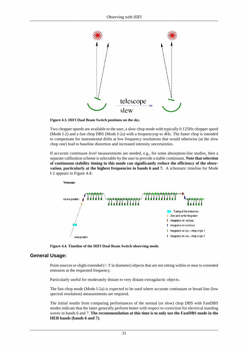
Observing with HIFI
31
Figure 4.3. HIFI Dual Beam Switch positions on the sky.
Two chopper speeds are available to the user, a slow chop mode with typically 0.125Hz chopper speed(Mode I-2) and a fast chop DBS (Mode I-2a) with a frequencyup to 4Hz. The faster chop is intendedto compensate for instrumental drifts at low frequency resolutions that would otherwise (at the slowchop rate) lead to baseline distortion and increased intensity uncertainties.
If accurate continuum level measurements are needed, e.g., for some absorption-line studies, then aseparate calibration scheme is selectable by the user to provide a stable continuum. Note that selectionof continuum stability timing in this mode can significantly reduce the efficiency of the obser-vation, particularly at the highest frequencies in bands 6 and 7. A schematic timeline for ModeI-2 appears in Figure 4.4:
Figure 4.4. Timeline of the HIFI Dual Beam Switch observing mode.
General Usage:
Point sources or slight extended (< 3' in diameter) objects that are not sitting within or near to extendedemission at the requested frequency.
Particularly useful for moderately distant to very distant extragalactic objects.
The fast chop mode (Mode I-2a) is expected to be used where accurate continuum or broad line (lowspectral resolution) measurements are required.
The initial results from comparing performances of the normal (or slow) chop DBS with FastDBSmodes indicate that the latter generally perform better with respect to correction for electrical standingwaves in bands 6 and 7. The recommendation at this time is to only use the FastDBS mode in theHEB bands (bands 6 and 7).
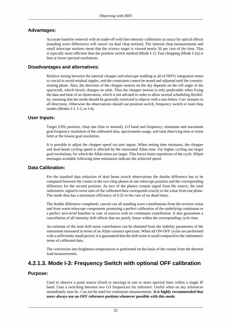
Observing with HIFI
32
Advantages:
Accurate baseline removal with no trade-off with line intensity calibration accuracy by optical effects(standing wave differences will cancel via dual chop motion). The internal chop measurements andsmall telescope motions mean that the science target is viewed nearly 50 per cent of the time. Thisis typically more efficient than the position switch method (Mode I-1). Fast chopping (Mode I-2a) isbest at lower spectral resolutions.
Disadvantages and alternatives:
Relative timing between the internal chopper and telescope nodding at all of HIFI's integration timesis crucial to avoid residual ripples, and the constraints cannot be tested and adjusted until the commis-sioning phase. Also, the direction of the chopper motion on the sky depends on the roll angle of thespacecraft, which slowly changes on orbit. Thus the chopper motion is only predictable when fixingthe data and time of an observation, which is not advised in order to allow normal scheduling flexibil-ity, meaning that the mode should be generally restricted to objects with a size below 3 arc minutes inall directions. Otherwise the observations should use position switch, frequency switch or load chopmodes (Modes I-1, I-3, or I-4).
User Inputs:
Target (ON) position, chop rate (fast or normal), LO band and frequency, minimum and maximumgoal frequency resolution of the calibrated data, spectrometer usage, and total observing time or noiselimit at the lowest goal resolution.
It is possible to adjust the chopper speed via user inputs. When setting time estimates, the chopperand dual-beam cycling speed is affected by the associated Allan time. For higher cycling use largergoal resolutions, for which the Allan times are larger. This forces faster repetitions of the cycle. HSpotmessages available following time estimation indicate the achieved speed.
Data Calibration:
For the standard data reduction of dual beam switch observations the double difference has to becomputed between the counts in the two chop phases at one telescope position and the correspondingdifference for the second position. As two of the phases contain signal from the source, the totalradiometric signal to noise ratio of the calibrated data corresponds exactly to the value from one phase.The mode thus has a maximum efficiency of 0.25 in the case of no dead times.
The double difference completely cancels out all standing wave contributions from the receiver noiseand from warm telescope components promising a perfect calibration of the underlying continuum ora perfect zero-level baseline in case of sources with no continuum contribution. It also guarantees acancellation of all intensity drift effects that are purely linear within the corresponding cycle time.
An estimate of the total drift noise contribution can be obtained from the stability parameters of theinstrument measured in terms of an Allan variance spectrum. When all ON-OFF cycles are performedwith a sufficiently small period, it is guaranteed that the drift noise is small compared to the radiometricnoise of calibrated data.
The conversion into brightness temperatures is performed on the basis of the counts from the thermalload measurements.
4.2.1.3. Mode I-3: Frequency Switch with optional OFF calibration
Purpose:
Used to observe a point source (fixed or moving) in one or more spectral lines within a single IFband. Uses a switching between two LO frequencies for reference. Useful when no sky referencesimmediately near by. Can not be used for continuum measurements. It is highly recommended thatusers always use an OFF reference position whenever possible with this mode.
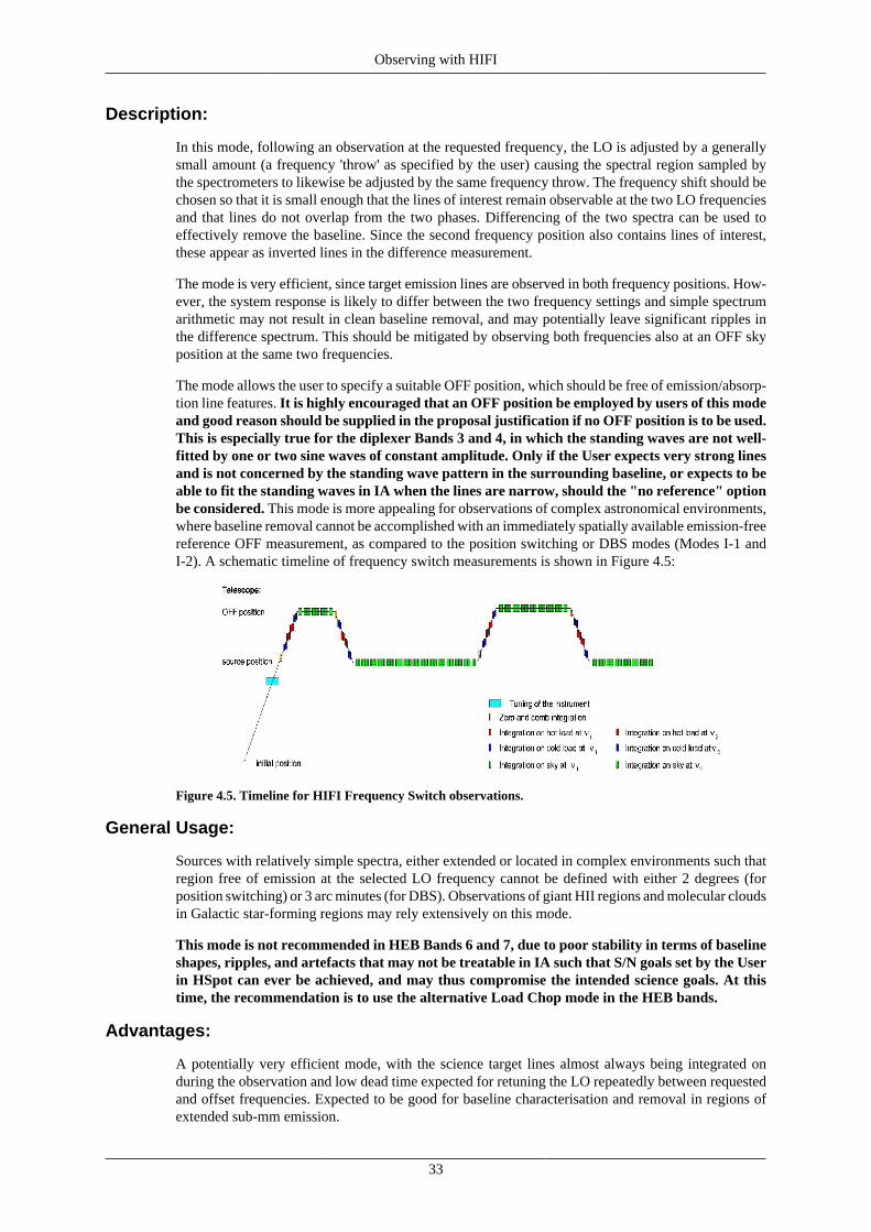
Observing with HIFI
33
Description:
In this mode, following an observation at the requested frequency, the LO is adjusted by a generallysmall amount (a frequency 'throw' as specified by the user) causing the spectral region sampled bythe spectrometers to likewise be adjusted by the same frequency throw. The frequency shift should bechosen so that it is small enough that the lines of interest remain observable at the two LO frequenciesand that lines do not overlap from the two phases. Differencing of the two spectra can be used toeffectively remove the baseline. Since the second frequency position also contains lines of interest,these appear as inverted lines in the difference measurement.
The mode is very efficient, since target emission lines are observed in both frequency positions. How-ever, the system response is likely to differ between the two frequency settings and simple spectrumarithmetic may not result in clean baseline removal, and may potentially leave significant ripples inthe difference spectrum. This should be mitigated by observing both frequencies also at an OFF skyposition at the same two frequencies.
The mode allows the user to specify a suitable OFF position, which should be free of emission/absorp-tion line features. It is highly encouraged that an OFF position be employed by users of this modeand good reason should be supplied in the proposal justification if no OFF position is to be used.This is especially true for the diplexer Bands 3 and 4, in which the standing waves are not well-fitted by one or two sine waves of constant amplitude. Only if the User expects very strong linesand is not concerned by the standing wave pattern in the surrounding baseline, or expects to beable to fit the standing waves in IA when the lines are narrow, should the "no reference" optionbe considered. This mode is more appealing for observations of complex astronomical environments,where baseline removal cannot be accomplished with an immediately spatially available emission-freereference OFF measurement, as compared to the position switching or DBS modes (Modes I-1 andI-2). A schematic timeline of frequency switch measurements is shown in Figure 4.5:
Figure 4.5. Timeline for HIFI Frequency Switch observations.
General Usage:
Sources with relatively simple spectra, either extended or located in complex environments such thatregion free of emission at the selected LO frequency cannot be defined with either 2 degrees (forposition switching) or 3 arc minutes (for DBS). Observations of giant HII regions and molecular cloudsin Galactic star-forming regions may rely extensively on this mode.
This mode is not recommended in HEB Bands 6 and 7, due to poor stability in terms of baselineshapes, ripples, and artefacts that may not be treatable in IA such that S/N goals set by the Userin HSpot can ever be achieved, and may thus compromise the intended science goals. At thistime, the recommendation is to use the alternative Load Chop mode in the HEB bands.
Advantages:
A potentially very efficient mode, with the science target lines almost always being integrated onduring the observation and low dead time expected for retuning the LO repeatedly between requestedand offset frequencies. Expected to be good for baseline characterisation and removal in regions ofextended sub-mm emission.
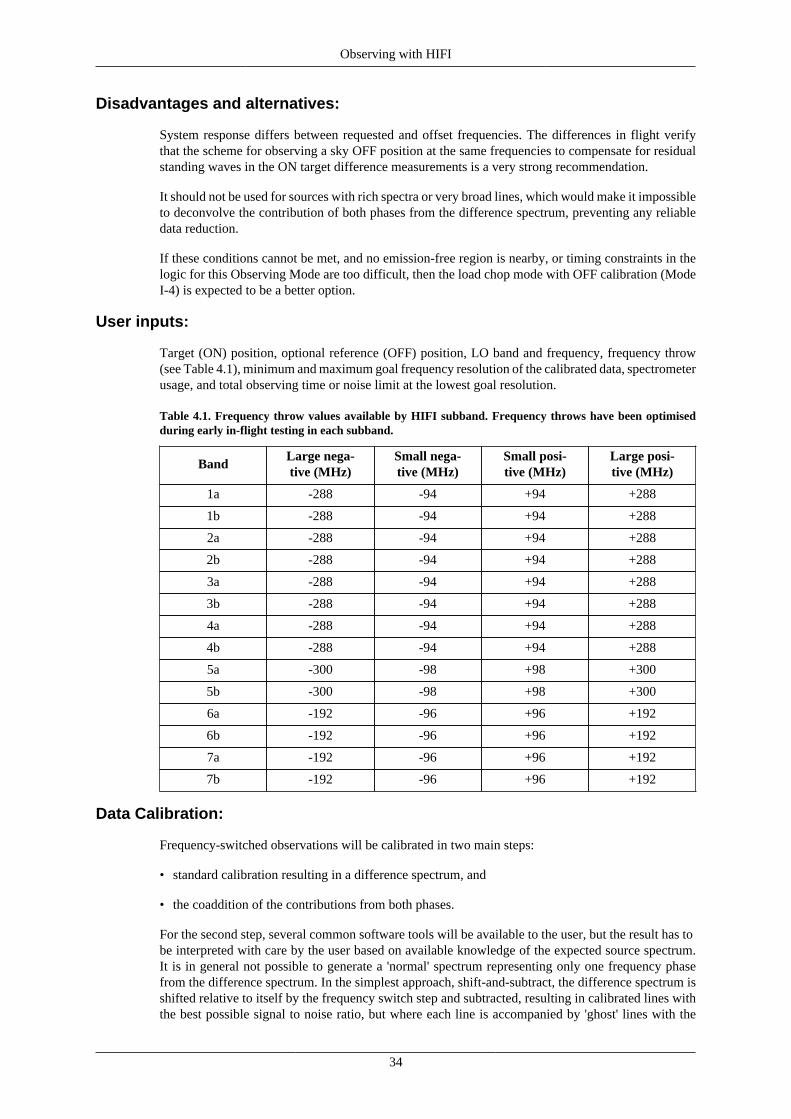
Observing with HIFI
34
Disadvantages and alternatives:
System response differs between requested and offset frequencies. The differences in flight verifythat the scheme for observing a sky OFF position at the same frequencies to compensate for residualstanding waves in the ON target difference measurements is a very strong recommendation.
It should not be used for sources with rich spectra or very broad lines, which would make it impossibleto deconvolve the contribution of both phases from the difference spectrum, preventing any reliabledata reduction.
If these conditions cannot be met, and no emission-free region is nearby, or timing constraints in thelogic for this Observing Mode are too difficult, then the load chop mode with OFF calibration (ModeI-4) is expected to be a better option.
User inputs:
Target (ON) position, optional reference (OFF) position, LO band and frequency, frequency throw(see Table 4.1), minimum and maximum goal frequency resolution of the calibrated data, spectrometerusage, and total observing time or noise limit at the lowest goal resolution.
Table 4.1. Frequency throw values available by HIFI subband. Frequency throws have been optimisedduring early in-flight testing in each subband.
BandLarge nega-tive (MHz)
Small nega-tive (MHz)
Small posi-tive (MHz)
Large posi-tive (MHz)
1a -288 -94 +94 +288
1b -288 -94 +94 +288
2a -288 -94 +94 +288
2b -288 -94 +94 +288
3a -288 -94 +94 +288
3b -288 -94 +94 +288
4a -288 -94 +94 +288
4b -288 -94 +94 +288
5a -300 -98 +98 +300
5b -300 -98 +98 +300
6a -192 -96 +96 +192
6b -192 -96 +96 +192
7a -192 -96 +96 +192
7b -192 -96 +96 +192
Data Calibration:
Frequency-switched observations will be calibrated in two main steps:
• standard calibration resulting in a difference spectrum, and
• the coaddition of the contributions from both phases.
For the second step, several common software tools will be available to the user, but the result has tobe interpreted with care by the user based on available knowledge of the expected source spectrum.It is in general not possible to generate a 'normal' spectrum representing only one frequency phasefrom the difference spectrum. In the simplest approach, shift-and-subtract, the difference spectrum isshifted relative to itself by the frequency switch step and subtracted, resulting in calibrated lines withthe best possible signal to noise ratio, but where each line is accompanied by 'ghost' lines with the
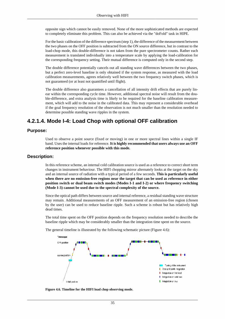
Observing with HIFI
35
opposite sign which cannot be easily removed. None of the more sophisticated methods are expectedto completely eliminate this problem. This can also be achieved via the "doFold" task in HIPE.
For the basic calibration of the difference spectrum (step 1), the difference of the measurement betweenthe two phases on the OFF position is subtracted from the ON source difference, but in contrast to theload-chop mode, this double-difference is not taken from the pure spectrometer counts. Rather eachmeasurement is translated individually into a temperature scale by applying the load-calibration forthe corresponding frequency setting. Their mutual difference is computed only in the second step.
The double difference potentially cancels out all standing wave differences between the two phases,but a perfect zero-level baseline is only obtained if the system response, as measured with the loadcalibration measurements, agrees relatively well between the two frequency switch phases, which isnot guaranteed (or at least not quantified until flight).
The double difference also guarantees a cancellation of all intensity drift effects that are purely lin-ear within the corresponding cycle time. However, additional spectral noise will result from the dou-ble-difference, and extra analysis time is likely to be required for the baseline calibration measure-ment, which will add to the noise in the calibrated data. This may represent a considerable overheadif the goal frequency resolution of the observation is not much smaller than the resolution needed todetermine possible standing wave ripples in the system.
4.2.1.4. Mode I-4: Load Chop with optional OFF calibration
Purpose:
Used to observe a point source (fixed or moving) in one or more spectral lines within a single IFband. Uses the internal loads for reference. It is highly recommended that users always use an OFFreference position whenever possible with this mode.
Description:
In this reference scheme, an internal cold calibration source is used as a reference to correct short termchanges in instrument behaviour. The HIFI chopping mirror alternately looks at the target on the skyand an internal source of radiation with a typical period of a few seconds. This is particularly usefulwhen there are no emission-free regions near the target that can be used as reference in eitherposition switch or dual beam switch modes (Modes I-1 and I-2) or where frequency switching(Mode I-3) cannot be used due to the spectral complexity of the source.
Since the optical path differs between source and internal reference, a residual standing wave structuremay remain. Additional measurements of an OFF measurement of an emission-free region (chosenby the user) can be used to reduce baseline ripple. Such a scheme is robust but has relatively highdead times.
The total time spent on the OFF position depends on the frequency resolution needed to describe thebaseline ripple which may be considerably smaller than the integration time spent on the source.
The general timeline is illustrated by the following schematic picture (Figure 4.6):
Figure 4.6. Timeline for the HIFI load chop observing mode.
Observing with HIFI
36
General Usage:
Sources with a high density of emission/absorption lines that lie within extended emitting regions. Likethe Frequency Switch mode, Load Chop is recommended to be used only with the sky referenceoption to obtain a spectrum at a User-selected line-free region (within 2 degrees of the science target)for standing wave correction in the pipeline. This applies most strongly to Bands 3, 4, 6, and 7, and/or in cases where lines may be too broad for interactive ripple fitting.
Advantages:
This is an efficient mode for measurements of sources in extended emission regions. With OFF refer-ence, the mode can be used as a fall-back for observations that would normally use a position switchbut where the distance to the OFF position would require a slew time comparable to the total on sourceintegration time. With use of an OFF position, in principle, all pointed observations could be donewith this robust mode, at the expense of higher dead times.
Disadvantages and alternatives:
Generally inefficient with typically 1/3 to 1/4 of the total time spent on the actual science target (timeon the OFF position is less than that on the target). However, this is a mode which attempts to providerobust calibration of data for the most spatially and spectrally complex targets in single pointing modes,and therefore no further alternatives are offered.
User inputs:
Target (ON) position, optional reference (OFF) position, LO band and frequency, minimum and max-imum goal frequency resolution of the calibrated data, spectrometer usage, and total observing timeor noise limit at the lowest goal resolution.
Data calibration:
The observing mode of load-chop observations with an OFF calibration is extremely robust with re-spect to calibration uncertainties, because it uses a double difference to determine the flux from theastronomical source relative to the flux from the sky on the OFF position. The double difference com-pletely cancels out all uncertainties in standing wave contributions from the receiver noise and fromwarm telescope components, promising a perfect calibration of the underlying continuum or a perfectzero-level baseline in case of sources with no continuum contribution.
The mode also guarantees a cancellation of all intensity drift effects that are purely linear within thecorresponding cycle time.
This robustness is, however, obtained at the cost of an increased spectral noise produced by the dou-ble-difference. If the period of standing waves in the system is equal to or less than the desired fre-quency resolution of the observations, the observing time has to be doubled to obtain the same sig-nal-to-noise ratio as compared to observations without baseline calibration. Many observations will,however, require a frequency resolution that is finer than the standing wave ripple so that the overheadfrom the baseline calibration is smaller.
If the user chooses to opt out of the OFF reference measurement, then a residual baseline (includingripple) is likely to remain and may require removal interactively by the user.
4.2.2. Modes of the Mapping AOT IIThere are four mapping modes available to HIFI. The "On-the-Fly" observing mode takes data con-tinuously as a source is scanned and can use a frequency switch reference, a load chop reference or asky reference, while a dual beam switch (DBS) raster map takes data at set points on a user-definedgrid. A variant of the DBS raster map, a small 5-point raster cross map was originally made availablebut has now been discontinued.
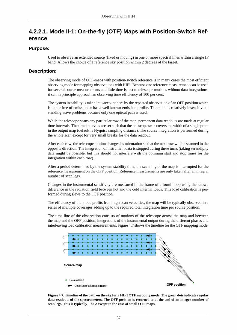
Observing with HIFI
37
4.2.2.1. Mode II-1: On-the-fly (OTF) Maps with Position-Switch Ref-erence
Purpose:
Used to observe an extended source (fixed or moving) in one or more spectral lines within a single IFband. Allows the choice of a reference sky position within 2 degrees of the target.
Description:
The observing mode of OTF-maps with position-switch reference is in many cases the most efficientobserving mode for mapping observations with HIFI. Because one reference measurement can be usedfor several source measurements and little time is lost to telescope motions without data integrations,it can in principle approach an observing time efficiency of 100 per cent.
The system instability is taken into account here by the repeated observation of an OFF position whichis either free of emission or has a well known emission profile. The mode is relatively insensitive tostanding wave problems because only one optical path is used.
While the telescope scans any particular row of the map, permanent data readouts are made at regulartime intervals. The time intervals are set such that the telescope scan covers the width of a single pointin the output map (default is Nyquist sampling distance). The source integration is performed duringthe whole scan except for very small breaks for the data readout.
After each row, the telescope motion changes its orientation so that the next row will be scanned in theopposite direction. The integration of instrument data is stopped during these turns (taking serendipitydata might be possible, but this should not interfere with the optimum start and stop times for theintegration within each row).
After a period determined by the system stability time, the scanning of the map is interrupted for thereference measurement on the OFF position. Reference measurements are only taken after an integralnumber of scan legs.
Changes in the instrumental sensitivity are measured in the frame of a fourth loop using the knowndifference in the radiation field between hot and the cold internal loads. This load calibration is per-formed during slews to the OFF position.
The efficiency of the mode profits from high scan velocities, the map will be typically observed in aseries of multiple coverages adding up to the required total integration time per source position.
The time line of the observation consists of motions of the telescope across the map and betweenthe map and the OFF position, integrations of the instrumental output during the different phases andinterleaving load calibration measurements. Figure 4.7 shows the timeline for the OTF mapping mode.
Figure 4.7. Timeline of the path on the sky for a HIFI OTF mapping mode. The green dots indicate regulardata readouts of the spectrometers. The OFF position is returned to at the end of an integer number ofscan legs. This is typically 1 or 2 except in the case of small OTF maps.
Observing with HIFI
38
In the example shown in Figure 4.7, the OFF position is visited three times within one coverage ofthe whole map, after every two scanned lines. It is planned to always complete full scan lines beforean OFF observation. A series of subsequent coverages will be performed with one extra OFF mea-surement at the end of the observation guaranteeing a complete enclosing of the source observationsby OFF observations. The green dots symbolise the points where the spectrometers are read out. Theintegration starts as soon as the telescope enters the blue area of the map. Note the change of thescanning direction after each row.
For situations where an emission-free OFF position is not immediately available, the OTF scan withload chop (scanning and comparing to frequent load measurements) or frequency switch (similarly,scanning and switching frequency) may preferably be used. This is particularly useful for mappingusing bands 6 and 7, where the short stability times mean that significant drifts can occur during amap scan leg. Continuous reference to the internal load during a scan leg (for example) can helpmitigate against such drifts and the increased associated with the drifts
Advantages:
On-the-Fly scanning should be considered the standard mode for astronomical mapping with HIFI. Itprovides the most efficient mapping scheme for HIFI. Load chop and frequency switch versions canbe useful in complex regions and when stability times are short (e.g., in the HEB bands, 6 and 7).
Disadvantages and Alternatives:
Its use is problematic if no nearby position can be defined for an OFF position which is free of emission.In this case it is often still possible and efficient to use an auxiliary nearby OFF position, the emissionof which is determined by a separate position-switch observation.
However, if the closest emission-free region is too distant from the area to be mapped, OTF modeswith frequency switch can be more efficient. The same holds in all cases where the scientific aimof the observation does not require an accurate treatment of baseline effects, ignoring standing waveripples or other baseline distortions. This will be the case for observations of very narrow lines whereeven a distorted baseline can be approximated by a simple linear profile across the line. In such casesOTF maps with frequency switch can be more efficient, but not good for broader lines, where the loadchop version of OTF is better.
It will not be possible to determine the continuum level from OTF maps. If continuum mapping (fora small region) is required then the DBS raster map should be used.
User inputs:
The user has the possibilities of rectangular map sizes, scan length (X) and cross-scan map size (Y).The cross-step can be set at Nyquist sampling or one of a number of set cross-step sizes (in arc seconds).The user is also asked for the position of an OFF reference source, which is mandatory.
Data calibration:
The reference for each scan map point is based on a combination of prior and following OFF positionmeasurements. Because of instrumental limitations with respect to data rates, the speed of the tele-scope motion, and the gain instabilities, it will not be possible to obtain an accurate determination ofthe continuum level from observations in OTF-maps with position switch reference. The subtractionof a zeroth order baseline should always be expected although the baseline itself does not need to becalibrated as the same optical path is used for source and reference. Observations aiming at a determi-nation of the continuum level have to rely on modes using the internal chopper such as the raster scan.
4.2.2.2. Mode II-2: Raster Maps with Dual Beam Switch
Purpose:
Used to observe a small an extended source (fixed or moving) in one or more spectral lines or con-tinuum within a single IF band. Uses the fixed 3' sky reference positions either side of each rasterposition which limits the effectively useful size of a raster.
Observing with HIFI
39
Description:
In this mode, a grid of positions are each measured using a dual beam switch method. The mode worksfor each grid position in the same way as for the point source dual beam switch mode (see Mode I-2).
The beam switch samples sky at 3 arc minutes either side of each grid position, with a telescopemovement occurring between changes to the beam switch either side of the grid position. With thissetup, large maps would find the beam chopping into the field of view, so this is not a good mode fordoing large extended emission region mapping.
Advantages:
It is a good mode for situations where fast (chopping) references are needed, as may be the casefor band 6 and 7 measurements, or where continuum measurements are required for small extendedsources or point sources. In these cases, scanning measurements may take too long allowing driftsto occur.
Disadvantages and Alternatives:
Not as efficient as OTF mapping and, with a beam switch of only 3 arc minutes, this is not a goodmode to use for large-scale maps.
Limited to 32x32 raster points in a single observation.
User inputs:
The user has the possibilities of rectangular map sizes, scan length (X) and cross-scan map size (Y).The cross-step can be set at Nyquist sampling or one of a number of set cross-step sizes (in arc seconds).Continuum timing (for accurate baseline measurements) and fast chopping are selectable.
Data calibration:
Each raster map position can be calibrated in the same way as single point dual beamswitch data (seeSection 4.2.1.2).
4.2.2.3. Mode II-2X: Cross Map with Dual Beam Switch (currentlyunavailable)
Purpose:
Used to observe spectral lines or continuum in a point source for which the most accurate flux is neededbut for which the position or pointing inaccuracy could cause significant error in the measurement.Uses sky references 3' either side of the target. Note that this mode is currently unavailable pendinga fix to its commanding -- it has had few science observation requests in the Key Project calls.
Description:
In this mode, a cross grid of set positions forming a 5-point cross are each measured using the dualbeam switch method. The separation of the cross positions is selectable as "pointing jitter" (to representthe possible worst-case pointing error of the observatory, currently set at 3"), "Nyquist" (for Nyquistsampling of the beam size for the chosen frequency), and "10", "20" or "40" arcseconds. The modeworks for each grid position in the same way as for the point source dual beam switch mode (seeMode I-2).
The beam switch samples sky at 3 arc minutes either side of each grid position, with a telescopemovement occurring between changes to the beam switch either side of the grid position.
Advantages:
Can improve the accuracy of flux measurements for point sources for any cases where the pointingerror or known position is large compared to the beam size.
Observing with HIFI
40
Provides basic flux and spatial information on small extended sources.
Disadvantages and Alternatives:
Can not be used for large maps and not a good means for obtaining accurate total flux information forextended sources. For accurate pointing and for objects with well known positions, some time is lostsince the telescope beam is slightly offset from the target position for each of the cross positions.
User inputs:
Continuum timing (for accurate baseline measurements) and fast chopping are also selectable.
Data calibration:
Each cross map position can be calibrated in the same way as single point dual beamswitch data (seeSection 4.2.1.2).
4.2.2.4. Mode II-3: OTF Maps with Frequency Switch
Description:
In this mode, a scan map is made across a source, during which frequency switching is introduced..The mode works for each scan map position in the same way as for the point source frequency switchmode (see Mode I-3).
Advantages:
It is a good mode for situations where fast (chopping) references are needed, as may be the case forband 6 and 7 measurements. An efficient mode for mapping of extended line emission regions sincetelescope slews to an OFF position are not necessary and the target grid positions are always beingmeasured (at slightly offset frequencies). Particularly useful for mapping large regions of line emissionwhere a DBS measurement (see Mode II-2) would have "contaminating" emission in the referencebeams.
Disadvantages and Alternatives:
The scheme has similar disadvantages to the single point frequency switch mode (see Section 4.2.1.3).System response will almost certainly be different at the requested and offset frequencies in a waywhich cannot be calculated from laboratory measurements. This may lead to residual standing waves.
User inputs:
The user has the possibilities of rectangular map sizes, scan length (X) and cross-scan map size (Y).The cross-step can be set at Nyquist sampling or one of a number of set cross-step sizes (in arc seconds).The frequency throw is selectable by the user.
Data calibration:
Each OTF map position can be calibrated in the same way as single point frequency switch data (seeSection 4.2.1.3).
4.2.2.5. Mode II-4: OTF Maps with Load Chop
Description:
In this mode, a scan map is made across a source, during which chopping against internal loads alsotakes place. The mode works for each scan map position in the same way as for the point source loadchop mode (see Mode I-4).
Observing with HIFI
41
Advantages:
It is a good mode for situations where fast (chopping) references are needed, as may be the case forband 6 and 7 measurements and for when frequency switching is made difficult by the density ofspectral lines or the expected existence of broad lines. It is an efficient mode for mapping of extendedline emission regions since telescope slews to an OFF position are not necessary and the target gridpositions are always being measured (at slightly offset frequencies). Particularly useful for mappinglarge regions of line emission where a DBS measurement (see Mode II-2) would have "contaminating"emission in the reference beams.
Disadvantages and Alternatives:
The scheme has similar disadvantages to the single point load chop mode (see Section 4.2.1.3). Thechanging light path between observing loads as opposed to the sky can lead to residual standing waves.
User inputs:
The user has the possibilities of rectangular map sizes, scan length (X) and cross-scan map size (Y).The cross-step can be set at Nyquist sampling or one of a number of set cross-step sizes (in arc seconds).
Data calibration:
Each OTF map position can be calibrated in the same way as single point load chop data (see Sec-tion 4.2.1.4).
4.2.3. Modes of the Spectral Scan AOT IIISpectral scans consist of a series of observations of a fixed single target at several frequencies usingthe WBS as main backend. After data processing, the result of such an observation will be a continuoussingle-sideband (SSB) spectrum for the selected position covering the selected frequency range. TheLO tuning will be advanced in small steps across a single LO band. From a data analysis standpoint,the reduction to a SSB spectrum is most reliable when the number of frequency settings within theinstantaneous bandwidth of the instrument is high, i.e. the frequency coverage is redundant. This mustbe balanced with the loss of observing efficiency imposed by the dead times associated with retuning toeach new LO frequency. For most sources, a reliable reduction of the line spectrum requires at least 5frequency settings within the IF bandwidth, i.e. a redundancy of 4. The spacings between the differentLO frequencies have to contain a small random component to prevent harmonics which could occurin the reduction of the multiple double-sideband measurements to a single sideband (SSB) spectrumin a deconvolution process.
This mode can use either a frequency switch (FS) or dual beam switch (DBS) reference frame tocompensate for instrumental drifts.
4.2.3.1. Mode III-2: Dual Beam Switch Spectral Scan
Purpose:
Used to observe a point source (fixed or moving) over a large frequency range (> 20GHz) by the useof multiple LO frequency settings during the observation. Uses the dual beam switch sky referencingscheme, sky positions 3' either side of the target.
Description:
The use of DBS reference inherits all the advantages and restrictions from the single point dual beamswitch observing mode (Mode I-2). The combination of telescope and chopper motions follows thesame scheme and timing constraints as Mode I-2. This implies also that this spectral scan mode canonly be applied to astronomical sources that are smaller than the chop angle of 3 arc minutes. Each LO
Observing with HIFI
42
frequency is separately calibrated against the internal hot/cold loads of the instrument. Extra observingtime is spent at LO frequencies where the system temperature is significantly degraded with respectto the rest of the LO subband being used.
The user may choose to do all or part of a spectral range within a given band.
NOTE: it is advised that the fast DBS chopping mode be used in association with bands 6 or 7 spectralscans.
Advantages:
Fast chop and continuum timing options allow for continuum measurements which are not possiblewith the frequency switch version of the spectral scan. Thus also the most useful for measuring ab-sorption line strengths.
Disadvantages and Alternatives:
The scheme has similar restrictions to other dual beam switch (DBS) measurements. For extendedsources the chopped beam is likely to land in an emission region. Fast chop is required when the sta-bility (Allan) times at the goal resolution of the system are less than 2 seconds. This reduces observingefficiency.
User inputs:
The user has choice of frequency range within the mixer band frequency range chosen (partial or fullband). The user can choose a redundancy of between 2 and 12. Higher values increase the fidelity ofthe final single sideband spectrum expected from the data reduction of the mode but also make themode less efficient. Fast chop and continuum timing for the DBS mode used are also available options.
Data calibration:
Data reduction consists of two parts: the calibration of the double sideband spectrum (see Sec-tion 4.2.1.2) and the deconvolution of the set of double sideband spectra into a single sideband spec-trum. The calibration of the double sideband spectrum is identical to the calibration in the single pointwith dual beam switch (see Section 4.2.1.2) applied for spectra taken at each LO setting
Sideband deconvolution is provided via a data software task provided within the HIPE software envi-ronment and takes place after each double sideband spectrum has been processed. More informationon the sideband deconvolution software are noted in Chapter 6.
No "ghost lines", symptoms of instabilities or insufficient sampling, have been found in any spectralsurvey so far. When spectral artefacts and bad baselines are removed completely from the input priorto using the deconvolution algorithm in post-processing, the deconvolution yields flat baselines withneither ringing, nor any added repetitive noise structures.
4.2.3.2. Mode III-3: Frequency Switch Spectral Scan
Purpose:
Used to observe a point source (fixed or moving) over a large frequency range (typically > 20GHz) bythe use of multiple LO frequency settings during the observation. But can also be used to get smallerranges where the different LO settings allow the distinguishing of spectral features into upper andlower sidebands. Uses frequency switching for reference.
Description:
This mode behaves in a similar fashion to the DBS version of mode III-2. The reference used is froma nearby frequency, using a small step frequency away from each of the main steps that are taken
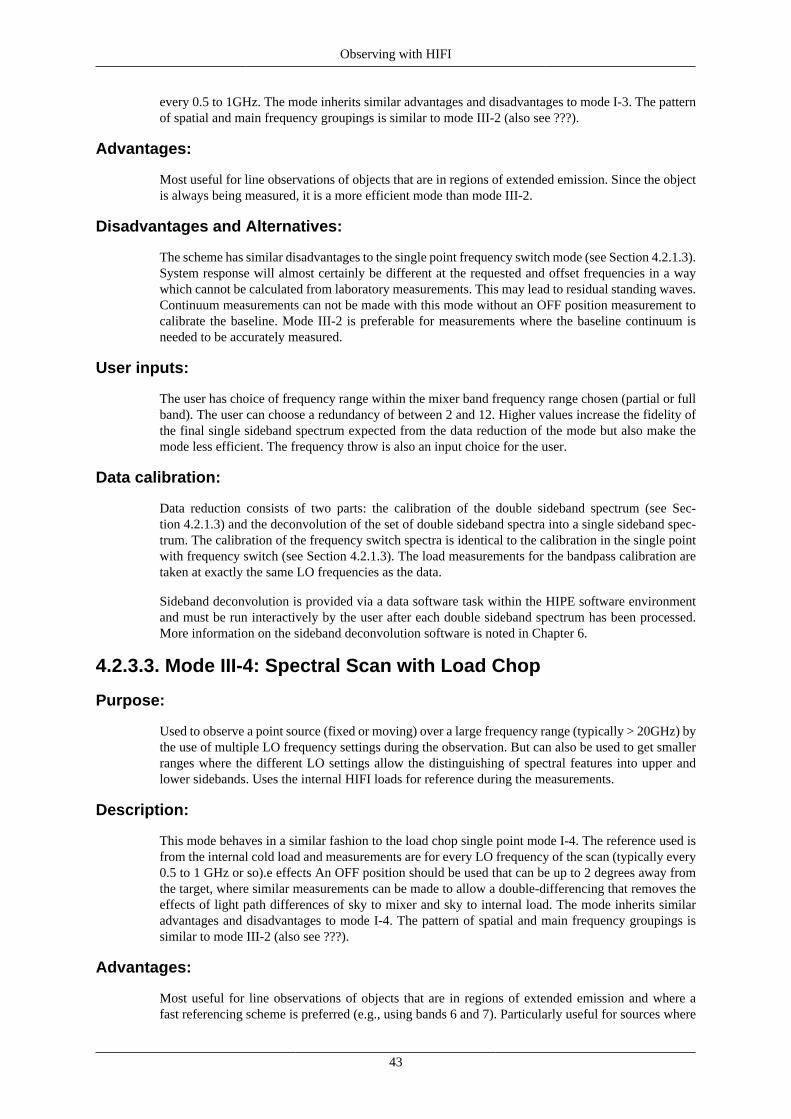
Observing with HIFI
43
every 0.5 to 1GHz. The mode inherits similar advantages and disadvantages to mode I-3. The patternof spatial and main frequency groupings is similar to mode III-2 (also see ???).
Advantages:
Most useful for line observations of objects that are in regions of extended emission. Since the objectis always being measured, it is a more efficient mode than mode III-2.
Disadvantages and Alternatives:
The scheme has similar disadvantages to the single point frequency switch mode (see Section 4.2.1.3).System response will almost certainly be different at the requested and offset frequencies in a waywhich cannot be calculated from laboratory measurements. This may lead to residual standing waves.Continuum measurements can not be made with this mode without an OFF position measurement tocalibrate the baseline. Mode III-2 is preferable for measurements where the baseline continuum isneeded to be accurately measured.
User inputs:
The user has choice of frequency range within the mixer band frequency range chosen (partial or fullband). The user can choose a redundancy of between 2 and 12. Higher values increase the fidelity ofthe final single sideband spectrum expected from the data reduction of the mode but also make themode less efficient. The frequency throw is also an input choice for the user.
Data calibration:
Data reduction consists of two parts: the calibration of the double sideband spectrum (see Sec-tion 4.2.1.3) and the deconvolution of the set of double sideband spectra into a single sideband spec-trum. The calibration of the frequency switch spectra is identical to the calibration in the single pointwith frequency switch (see Section 4.2.1.3). The load measurements for the bandpass calibration aretaken at exactly the same LO frequencies as the data.
Sideband deconvolution is provided via a data software task within the HIPE software environmentand must be run interactively by the user after each double sideband spectrum has been processed.More information on the sideband deconvolution software is noted in Chapter 6.
4.2.3.3. Mode III-4: Spectral Scan with Load Chop
Purpose:
Used to observe a point source (fixed or moving) over a large frequency range (typically > 20GHz) bythe use of multiple LO frequency settings during the observation. But can also be used to get smallerranges where the different LO settings allow the distinguishing of spectral features into upper andlower sidebands. Uses the internal HIFI loads for reference during the measurements.
Description:
This mode behaves in a similar fashion to the load chop single point mode I-4. The reference used isfrom the internal cold load and measurements are for every LO frequency of the scan (typically every0.5 to 1 GHz or so).e effects An OFF position should be used that can be up to 2 degrees away fromthe target, where similar measurements can be made to allow a double-differencing that removes theeffects of light path differences of sky to mixer and sky to internal load. The mode inherits similaradvantages and disadvantages to mode I-4. The pattern of spatial and main frequency groupings issimilar to mode III-2 (also see ???).
Advantages:
Most useful for line observations of objects that are in regions of extended emission and where afast referencing scheme is preferred (e.g., using bands 6 and 7). Particularly useful for sources where
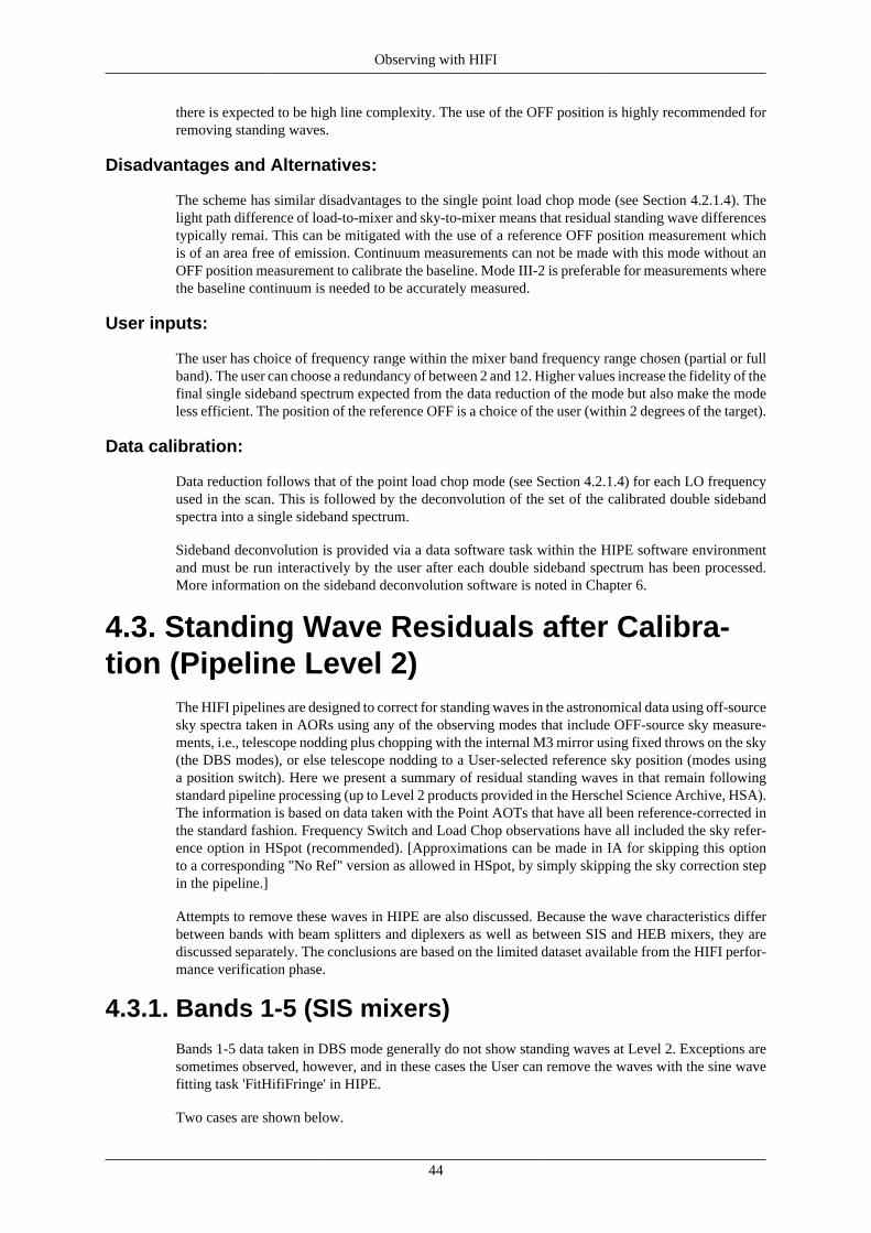
Observing with HIFI
44
there is expected to be high line complexity. The use of the OFF position is highly recommended forremoving standing waves.
Disadvantages and Alternatives:
The scheme has similar disadvantages to the single point load chop mode (see Section 4.2.1.4). Thelight path difference of load-to-mixer and sky-to-mixer means that residual standing wave differencestypically remai. This can be mitigated with the use of a reference OFF position measurement whichis of an area free of emission. Continuum measurements can not be made with this mode without anOFF position measurement to calibrate the baseline. Mode III-2 is preferable for measurements wherethe baseline continuum is needed to be accurately measured.
User inputs:
The user has choice of frequency range within the mixer band frequency range chosen (partial or fullband). The user can choose a redundancy of between 2 and 12. Higher values increase the fidelity of thefinal single sideband spectrum expected from the data reduction of the mode but also make the modeless efficient. The position of the reference OFF is a choice of the user (within 2 degrees of the target).
Data calibration:
Data reduction follows that of the point load chop mode (see Section 4.2.1.4) for each LO frequencyused in the scan. This is followed by the deconvolution of the set of the calibrated double sidebandspectra into a single sideband spectrum.
Sideband deconvolution is provided via a data software task within the HIPE software environmentand must be run interactively by the user after each double sideband spectrum has been processed.More information on the sideband deconvolution software is noted in Chapter 6.
4.3. Standing Wave Residuals after Calibra-tion (Pipeline Level 2)
The HIFI pipelines are designed to correct for standing waves in the astronomical data using off-sourcesky spectra taken in AORs using any of the observing modes that include OFF-source sky measure-ments, i.e., telescope nodding plus chopping with the internal M3 mirror using fixed throws on the sky(the DBS modes), or else telescope nodding to a User-selected reference sky position (modes usinga position switch). Here we present a summary of residual standing waves in that remain followingstandard pipeline processing (up to Level 2 products provided in the Herschel Science Archive, HSA).The information is based on data taken with the Point AOTs that have all been reference-corrected inthe standard fashion. Frequency Switch and Load Chop observations have all included the sky refer-ence option in HSpot (recommended). [Approximations can be made in IA for skipping this optionto a corresponding "No Ref" version as allowed in HSpot, by simply skipping the sky correction stepin the pipeline.]
Attempts to remove these waves in HIPE are also discussed. Because the wave characteristics differbetween bands with beam splitters and diplexers as well as between SIS and HEB mixers, they arediscussed separately. The conclusions are based on the limited dataset available from the HIFI perfor-mance verification phase.
4.3.1. Bands 1-5 (SIS mixers)Bands 1-5 data taken in DBS mode generally do not show standing waves at Level 2. Exceptions aresometimes observed, however, and in these cases the User can remove the waves with the sine wavefitting task 'FitHifiFringe' in HIPE.
Two cases are shown below.
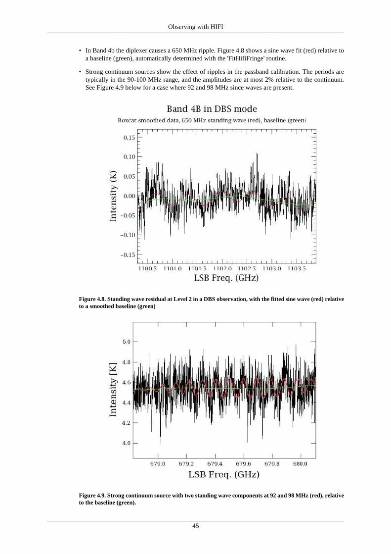
Observing with HIFI
45
• In Band 4b the diplexer causes a 650 MHz ripple. Figure 4.8 shows a sine wave fit (red) relative toa baseline (green), automatically determined with the 'FitHifiFringe' routine.
• Strong continuum sources show the effect of ripples in the passband calibration. The periods aretypically in the 90-100 MHz range, and the amplitudes are at most 2% relative to the continuum.See Figure 4.9 below for a case where 92 and 98 MHz since waves are present.
Figure 4.8. Standing wave residual at Level 2 in a DBS observation, with the fitted sine wave (red) relativeto a smoothed baseline (green)
Figure 4.9. Strong continuum source with two standing wave components at 92 and 98 MHz (red), relativeto the baseline (green).
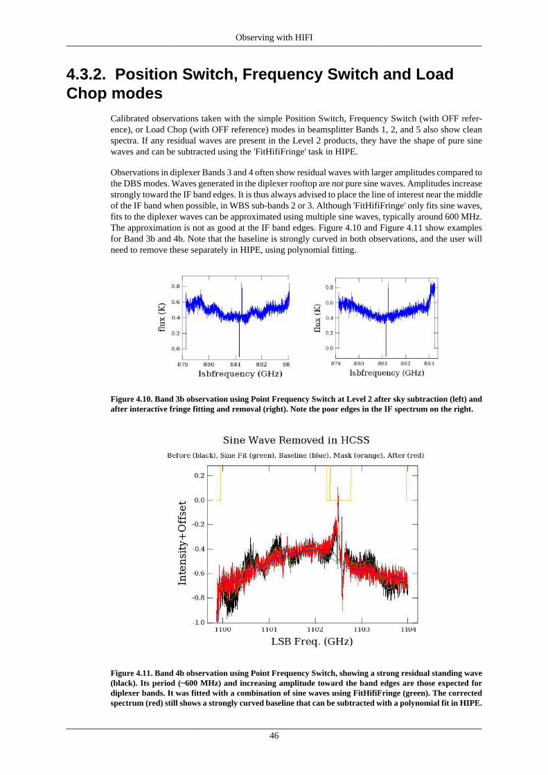
Observing with HIFI
46
4.3.2. Position Switch, Frequency Switch and LoadChop modes
Calibrated observations taken with the simple Position Switch, Frequency Switch (with OFF refer-ence), or Load Chop (with OFF reference) modes in beamsplitter Bands 1, 2, and 5 also show cleanspectra. If any residual waves are present in the Level 2 products, they have the shape of pure sinewaves and can be subtracted using the 'FitHifiFringe' task in HIPE.
Observations in diplexer Bands 3 and 4 often show residual waves with larger amplitudes compared tothe DBS modes. Waves generated in the diplexer rooftop are not pure sine waves. Amplitudes increasestrongly toward the IF band edges. It is thus always advised to place the line of interest near the middleof the IF band when possible, in WBS sub-bands 2 or 3. Although 'FitHifiFringe' only fits sine waves,fits to the diplexer waves can be approximated using multiple sine waves, typically around 600 MHz.The approximation is not as good at the IF band edges. Figure 4.10 and Figure 4.11 show examplesfor Band 3b and 4b. Note that the baseline is strongly curved in both observations, and the user willneed to remove these separately in HIPE, using polynomial fitting.
Figure 4.10. Band 3b observation using Point Frequency Switch at Level 2 after sky subtraction (left) andafter interactive fringe fitting and removal (right). Note the poor edges in the IF spectrum on the right.
Figure 4.11. Band 4b observation using Point Frequency Switch, showing a strong residual standing wave(black). Its period (~600 MHz) and increasing amplitude toward the band edges are those expected fordiplexer bands. It was fitted with a combination of sine waves using FitHifiFringe (green). The correctedspectrum (red) still shows a strongly curved baseline that can be subtracted with a polynomial fit in HIPE.
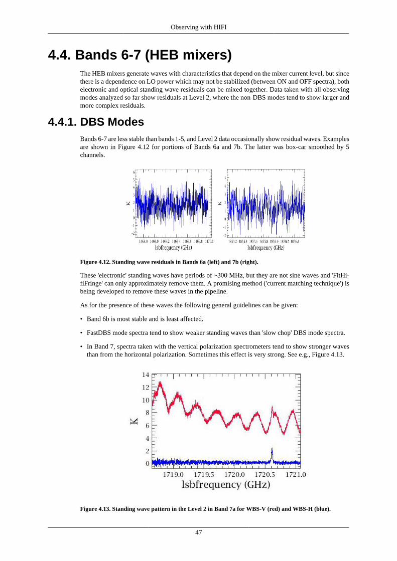
Observing with HIFI
47
4.4. Bands 6-7 (HEB mixers)The HEB mixers generate waves with characteristics that depend on the mixer current level, but sincethere is a dependence on LO power which may not be stabilized (between ON and OFF spectra), bothelectronic and optical standing wave residuals can be mixed together. Data taken with all observingmodes analyzed so far show residuals at Level 2, where the non-DBS modes tend to show larger andmore complex residuals.
4.4.1. DBS ModesBands 6-7 are less stable than bands 1-5, and Level 2 data occasionally show residual waves. Examplesare shown in Figure 4.12 for portions of Bands 6a and 7b. The latter was box-car smoothed by 5channels.
Figure 4.12. Standing wave residuals in Bands 6a (left) and 7b (right).
These 'electronic' standing waves have periods of ~300 MHz, but they are not sine waves and 'FitHi-fiFringe' can only approximately remove them. A promising method ('current matching technique') isbeing developed to remove these waves in the pipeline.
As for the presence of these waves the following general guidelines can be given:
• Band 6b is most stable and is least affected.
• FastDBS mode spectra tend to show weaker standing waves than 'slow chop' DBS mode spectra.
• In Band 7, spectra taken with the vertical polarization spectrometers tend to show stronger wavesthan from the horizontal polarization. Sometimes this effect is very strong. See e.g., Figure 4.13.
Figure 4.13. Standing wave pattern in the Level 2 in Band 7a for WBS-V (red) and WBS-H (blue).
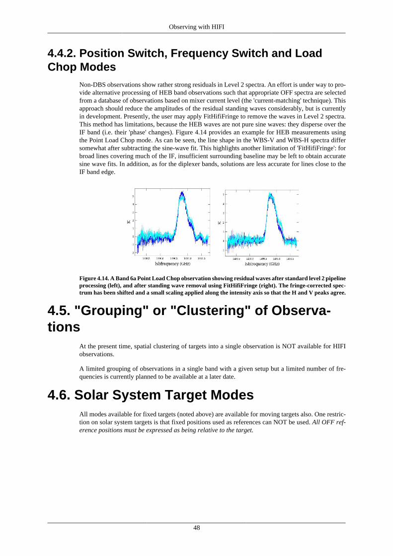
Observing with HIFI
48
4.4.2. Position Switch, Frequency Switch and LoadChop Modes
Non-DBS observations show rather strong residuals in Level 2 spectra. An effort is under way to pro-vide alternative processing of HEB band observations such that appropriate OFF spectra are selectedfrom a database of observations based on mixer current level (the 'current-matching' technique). Thisapproach should reduce the amplitudes of the residual standing waves considerably, but is currentlyin development. Presently, the user may apply FitHifiFringe to remove the waves in Level 2 spectra.This method has limitations, because the HEB waves are not pure sine waves: they disperse over theIF band (i.e. their 'phase' changes). Figure 4.14 provides an example for HEB measurements usingthe Point Load Chop mode. As can be seen, the line shape in the WBS-V and WBS-H spectra differsomewhat after subtracting the sine-wave fit. This highlights another limitation of 'FitHifiFringe': forbroad lines covering much of the IF, insufficient surrounding baseline may be left to obtain accuratesine wave fits. In addition, as for the diplexer bands, solutions are less accurate for lines close to theIF band edge.
Figure 4.14. A Band 6a Point Load Chop observation showing residual waves after standard level 2 pipelineprocessing (left), and after standing wave removal using FitHifiFringe (right). The fringe-corrected spec-trum has been shifted and a small scaling applied along the intensity axis so that the H and V peaks agree.
4.5. "Grouping" or "Clustering" of Observa-tions
At the present time, spatial clustering of targets into a single observation is NOT available for HIFIobservations.
A limited grouping of observations in a single band with a given setup but a limited number of fre-quencies is currently planned to be available at a later date.
4.6. Solar System Target ModesAll modes available for fixed targets (noted above) are available for moving targets also. One restric-tion on solar system targets is that fixed positions used as references can NOT be used. All OFF ref-erence positions must be expressed as being relative to the target.
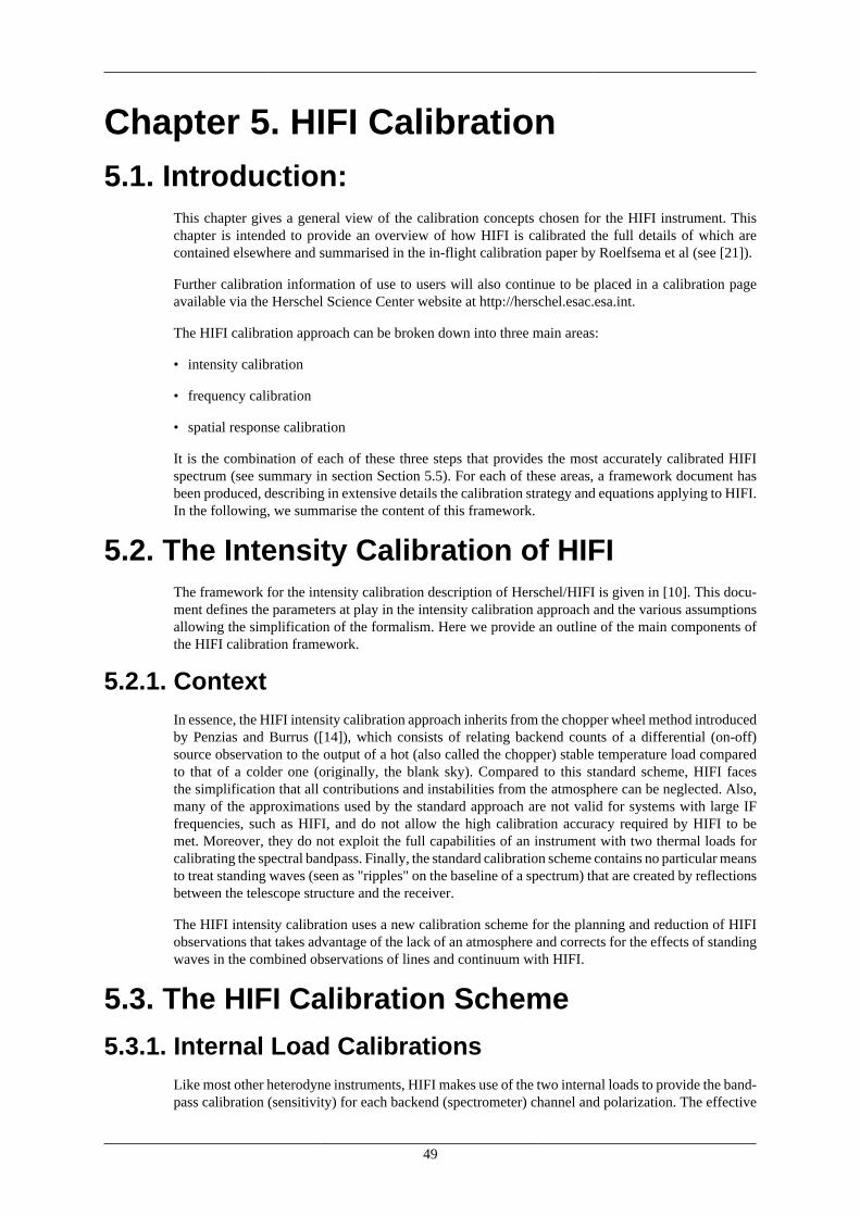
49
Chapter 5. HIFI Calibration5.1. Introduction:
This chapter gives a general view of the calibration concepts chosen for the HIFI instrument. Thischapter is intended to provide an overview of how HIFI is calibrated the full details of which arecontained elsewhere and summarised in the in-flight calibration paper by Roelfsema et al (see [21]).
Further calibration information of use to users will also continue to be placed in a calibration pageavailable via the Herschel Science Center website at http://herschel.esac.esa.int.
The HIFI calibration approach can be broken down into three main areas:
• intensity calibration
• frequency calibration
• spatial response calibration
It is the combination of each of these three steps that provides the most accurately calibrated HIFIspectrum (see summary in section Section 5.5). For each of these areas, a framework document hasbeen produced, describing in extensive details the calibration strategy and equations applying to HIFI.In the following, we summarise the content of this framework.
5.2. The Intensity Calibration of HIFIThe framework for the intensity calibration description of Herschel/HIFI is given in [10]. This docu-ment defines the parameters at play in the intensity calibration approach and the various assumptionsallowing the simplification of the formalism. Here we provide an outline of the main components ofthe HIFI calibration framework.
5.2.1. ContextIn essence, the HIFI intensity calibration approach inherits from the chopper wheel method introducedby Penzias and Burrus ([14]), which consists of relating backend counts of a differential (on-off)source observation to the output of a hot (also called the chopper) stable temperature load comparedto that of a colder one (originally, the blank sky). Compared to this standard scheme, HIFI facesthe simplification that all contributions and instabilities from the atmosphere can be neglected. Also,many of the approximations used by the standard approach are not valid for systems with large IFfrequencies, such as HIFI, and do not allow the high calibration accuracy required by HIFI to bemet. Moreover, they do not exploit the full capabilities of an instrument with two thermal loads forcalibrating the spectral bandpass. Finally, the standard calibration scheme contains no particular meansto treat standing waves (seen as "ripples" on the baseline of a spectrum) that are created by reflectionsbetween the telescope structure and the receiver.
The HIFI intensity calibration uses a new calibration scheme for the planning and reduction of HIFIobservations that takes advantage of the lack of an atmosphere and corrects for the effects of standingwaves in the combined observations of lines and continuum with HIFI.
5.3. The HIFI Calibration Scheme
5.3.1. Internal Load CalibrationsLike most other heterodyne instruments, HIFI makes use of the two internal loads to provide the band-pass calibration (sensitivity) for each backend (spectrometer) channel and polarization. The effective
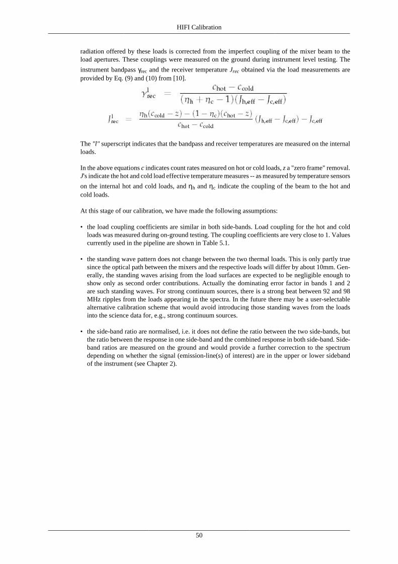
HIFI Calibration
50
radiation offered by these loads is corrected from the imperfect coupling of the mixer beam to theload apertures. These couplings were measured on the ground during instrument level testing. The
instrument bandpass γrec and the receiver temperature Jrec obtained via the load measurements areprovided by Eq. (9) and (10) from [10].
The "l" superscript indicates that the bandpass and receiver temperatures are measured on the internalloads.
In the above equations c indicates count rates measured on hot or cold loads, z a "zero frame" removal.J's indicate the hot and cold load effective temperature measures -- as measured by temperature sensors
on the internal hot and cold loads, and ηh and ηc indicate the coupling of the beam to the hot andcold loads.
At this stage of our calibration, we have made the following assumptions:
• the load coupling coefficients are similar in both side-bands. Load coupling for the hot and coldloads was measured during on-ground testing. The coupling coefficients are very close to 1. Valuescurrently used in the pipeline are shown in Table 5.1.
• the standing wave pattern does not change between the two thermal loads. This is only partly truesince the optical path between the mixers and the respective loads will differ by about 10mm. Gen-erally, the standing waves arising from the load surfaces are expected to be negligible enough toshow only as second order contributions. Actually the dominating error factor in bands 1 and 2are such standing waves. For strong continuum sources, there is a strong beat between 92 and 98MHz ripples from the loads appearing in the spectra. In the future there may be a user-selectablealternative calibration scheme that would avoid introducing those standing waves from the loadsinto the science data for, e.g., strong continuum sources.
• the side-band ratio are normalised, i.e. it does not define the ratio between the two side-bands, butthe ratio between the response in one side-band and the combined response in both side-band. Side-band ratios are measured on the ground and would provide a further correction to the spectrumdepending on whether the signal (emission-line(s) of interest) are in the upper or lower sidebandof the instrument (see Chapter 2).
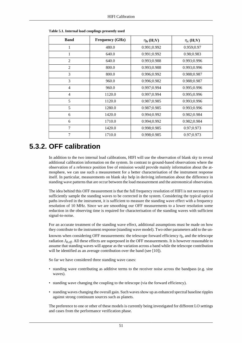
HIFI Calibration
51
Table 5.1. Internal load couplings presently used
Band Frequency (GHz) ηh (H;V) ηc (H;V)
1 480.0 0.991;0.992 0.959;0.97
1 640.0 0.991;0.992 0.98;0.983
2 640.0 0.993;0.988 0.993;0.996
2 800.0 0.993;0.988 0.993;0.996
3 800.0 0.996;0.992 0.988;0.987
3 960.0 0.996;0.982 0.988;0.987
4 960.0 0.997;0.994 0.995;0.996
4 1120.0 0.997;0.994 0.995;0.996
5 1120.0 0.987;0.985 0.993;0.996
5 1280.0 0.987;0.985 0.993;0.996
6 1420.0 0.994;0.992 0.982;0.984
6 1710.0 0.994;0.992 0.982;0.984
7 1420.0 0.998;0.985 0.97;0.973
7 1710.0 0.998;0.985 0.97;0.973
5.3.2. OFF calibrationIn addition to the two internal load calibrations, HIFI will use the observation of blank sky to revealadditional calibration information on the system. In contrast to ground-based observations where theobservation of a reference position free of emission would provide mainly information about the at-mosphere, we can use such a measurement for a better characterisation of the instrument responseitself. In particular, measurements on blank sky help in deriving information about the difference instanding wave patterns that are occur between the load measurement and the astronomical observation.
The idea behind this OFF measurement is that the full frequency resolution of HIFI is not necessary tosufficiently sample the standing waves to be corrected in the system. Considering the typical opticalpaths involved in the instrument, it is sufficient to measure the standing wave effect with a frequencyresolution of 10 MHz. Since we are smoothing our OFF measurements to a lower resolution somereduction in the observing time is required for characterisation of the standing waves with sufficientsignal-to-noise.
For an accurate treatment of the standing wave effect, additional assumptions must be made on howthey contribute to the instrument response (standing wave model). Two other parameters add to the un-
knowns when considering OFF measurements: the telescope forward efficiency ηl, and the telescoperadiation JR,eff. All these effects are superposed in the OFF measurements. It is however reasonable toassume that standing waves will appear as the variation across a band while the telescope contributionwill be identified as an average contribution over the band (see [10]).
So far we have considered three standing wave cases:
• standing wave contributing as additive terms to the receiver noise across the bandpass (e.g. sinewaves).
• standing wave changing the coupling to the telescope (via the forward efficiency).
• standing waves changing the overall gain. Such waves show up as enhanced spectral baseline ripplesagainst strong continuum sources such as planets.
The preference to one or other of these models is currently being investigated for different LO settingsand cases from the performance verification phase.
HIFI Calibration
52
5.3.3. Differencing observations:To correct for instrument drift effects, the astronomical observations will use a differencing schemewhere the astronomical source and a reference are observed in an alternating sequence. HIFI usesfour basic approaches: total power (also called Position Switch), sky chop (also called Double BeamSwitch), load chop and frequency switch (see chapter on observing modes). Reference [10] gives someexamples of the equations obtained in various differencing schemes, and depending on the standingwave model approach. In particular, it shows how both line and continuum contributions to the signalcan be separately treated. The continuum term only contains the radiation from the source and theblank sky in its surrounding. The continuum radiation seen from the warm telescope structure cancelsout in all equations by means of the OFF calibration.
In essence, the OFF calibration combined to the differencing approach always provides a double dif-ference. The double difference corrects for the standing waves in the baselines but from the pointof view of observational noise, ON and OFF measurements are equivalent. Thus the use of an OFFcalibration may be less efficient that total power measurements. This is depending on the system sta-bility, which could offer the possibility to use one OFF calibration measurement for a series of sourcemeasurement.
5.3.4. Non-linearity:In all equations and references mentioned above, it has been assumed that the instrument response toany radiation field is linear. Deviations from a linear behaviour are expected mainly in the IF branchincluding the spectrometers. However from ground-based measurements, it was concluded that thesedeviations are not significant (1% or less), and can in any case be measured and corrected in the dataprocessing.
5.3.5. Blank-sky contribution:The main contribution from the blank sky comes from the dust emission in the Milky Way, which isthe brightest extended source of radiation in the considered wavelength region. For a typical GalacticOFF position 4-5 degrees from the Galactic plane at 500 GHz, the continuum intensity correspondsto 10-3 K, and thus is far from having any noticeable influence. In sky regions closer to the Galacticplane, the continuum intensity increases but remains insignificant. Only in the direction of the Galacticcentre the continuum emission becomes no longer negligible. These numbers are based on the workof Schlegel et al. ([15]) who obtained the spatial distribution of the dusty density and temperaturecombining IRAS and DIRBE data.
5.3.6. Conversion between Antenna Temperature andJanskys:
The HIFI calibrated product, as obtained from the pipeline, is provided in antenna temperature (TA).To convert this to a source flux in Janskys requires some knowledge of the beam at the frequencyused. HIFI beam information is discussed in Section 5.5.2. The formula for conversion is:
S/TA = 326.9/ηA Jy/K
The value of ηA for each subband is listed in Table 5.5.
5.4. The Frequency Calibration of HIFI:The framework for the frequency calibration description of Herschel/HIFI is given in [11]. This doc-ument presents the terminology related to this topic, and recalls the principles and parameters to con-sider for the HIFI frequency calibration. Some of these parameters have already been introduced inthe spectrometer description sections (see Chapter 2).
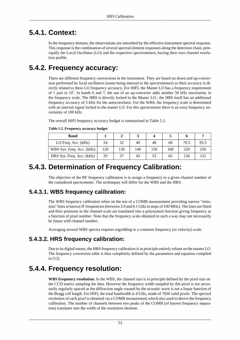
HIFI Calibration
53
5.4.1. Context:In the frequency domain, the observations are smoothed by the effective instrument spectral response.This response is the combination of several spectral element responses along the detection chain, prin-cipally the Local Oscillator (LO) and the respective spectrometers, having their own channel resolu-tion profile.
5.4.2. Frequency accuracy:There are different frequency conversions in the instrument. They are based on down and up-conver-sion performed by local oscillators (some being internal to the spectrometers) so their accuracy is di-rectly related to these LO frequency accuracy. For HIFI, the Master LO has a frequency requirementof 1 part in 107. In bands 6 and 7, the use of an up-converter adds another 50 kHz uncertainty inthe frequency scale. The HRS is directly locked to the Master LO ; the HRS itself has an additionalfrequency accuracy of 5 kHz for the autocorrelator. For the WBS, the frequency scale is determinedwith an internal signal locked to the master LO. For this spectrometer there is an extra frequency un-certainty of 100 kHz.
The overall HIFI frequency accuracy budget is summarised in Table 5.2.
Table 5.2. Frequency accuracy budget
Band 1 2 3 4 5 6 7
LO Freq. Acc. (kHz) 24 32 40 48 60 70.5 95.5
WBS Sys. Freq. Acc. (kHz) 120 130 140 150 160 220 250
HRS Sys. Freq. Acc. (kHz) 29 37 45 53 65 126 151
5.4.3. Determination of Frequency Calibration:The objective of the RF frequency calibration is to assign a frequency to a given channel number ofthe considered spectrometer. The techniques will differ for the WBS and the HRS:
5.4.3.1. WBS frequency calibration:
The WBS frequency calibration relies on the use of a COMB measurement providing narrow "emis-sion" lines at known IF frequencies (between 3.9 and 8.1 GHz in steps of 100 MHz). The lines are fittedand their positions in the channel scale are translated into a polynomial function giving frequency asa function of pixel number. Note that the frequency scale obtained in such a way may not necessarilybe linear with channel number.
Averaging several WBS spectra requires regridding to a common frequency (or velocity) scale.
5.4.3.2. HRS frequency calibration:
Due to its digital nature, the HRS frequency calibration is in principle entirely reliant on the master LO.The frequency conversion table is thus completely defined by the parameters and equation compiledin [12].
5.4.4. Frequency resolution:WBS frequency resolution: In the WBS, the channel size is in principle defined by the pixel size onthe CCD matrix sampling the data. However the frequency width sampled by this pixel is not neces-sarily regularly spaced as the diffraction angle created by the acoustic wave is not a linear function ofthe Bragg cell length. For HIFI, the total bandwidth is 4 GHz, made of 7650 valid pixels. The spectralresolution of each pixel is obtained via a COMB measurement which also used to derive the frequencycalibration. The number of channels between two peaks of the COMB (of known frequency separa-tion) translates into the width of the resolution element.
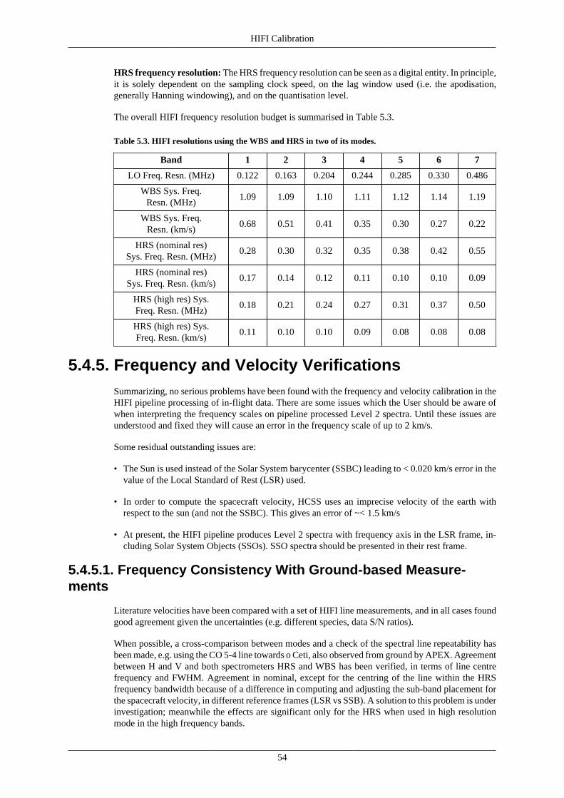
HIFI Calibration
54
HRS frequency resolution: The HRS frequency resolution can be seen as a digital entity. In principle,it is solely dependent on the sampling clock speed, on the lag window used (i.e. the apodisation,generally Hanning windowing), and on the quantisation level.
The overall HIFI frequency resolution budget is summarised in Table 5.3.
Table 5.3. HIFI resolutions using the WBS and HRS in two of its modes.
Band 1 2 3 4 5 6 7
LO Freq. Resn. (MHz) 0.122 0.163 0.204 0.244 0.285 0.330 0.486
WBS Sys. Freq.Resn. (MHz)
1.09 1.09 1.10 1.11 1.12 1.14 1.19
WBS Sys. Freq.Resn. (km/s)
0.68 0.51 0.41 0.35 0.30 0.27 0.22
HRS (nominal res)Sys. Freq. Resn. (MHz)
0.28 0.30 0.32 0.35 0.38 0.42 0.55
HRS (nominal res)Sys. Freq. Resn. (km/s)
0.17 0.14 0.12 0.11 0.10 0.10 0.09
HRS (high res) Sys.Freq. Resn. (MHz)
0.18 0.21 0.24 0.27 0.31 0.37 0.50
HRS (high res) Sys.Freq. Resn. (km/s)
0.11 0.10 0.10 0.09 0.08 0.08 0.08
5.4.5. Frequency and Velocity VerificationsSummarizing, no serious problems have been found with the frequency and velocity calibration in theHIFI pipeline processing of in-flight data. There are some issues which the User should be aware ofwhen interpreting the frequency scales on pipeline processed Level 2 spectra. Until these issues areunderstood and fixed they will cause an error in the frequency scale of up to 2 km/s.
Some residual outstanding issues are:
• The Sun is used instead of the Solar System barycenter (SSBC) leading to < 0.020 km/s error in thevalue of the Local Standard of Rest (LSR) used.
• In order to compute the spacecraft velocity, HCSS uses an imprecise velocity of the earth withrespect to the sun (and not the SSBC). This gives an error of ~< 1.5 km/s
• At present, the HIFI pipeline produces Level 2 spectra with frequency axis in the LSR frame, in-cluding Solar System Objects (SSOs). SSO spectra should be presented in their rest frame.
5.4.5.1. Frequency Consistency With Ground-based Measure-ments
Literature velocities have been compared with a set of HIFI line measurements, and in all cases foundgood agreement given the uncertainties (e.g. different species, data S/N ratios).
When possible, a cross-comparison between modes and a check of the spectral line repeatability hasbeen made, e.g. using the CO 5-4 line towards o Ceti, also observed from ground by APEX. Agreementbetween H and V and both spectrometers HRS and WBS has been verified, in terms of line centrefrequency and FWHM. Agreement in nominal, except for the centring of the line within the HRSfrequency bandwidth because of a difference in computing and adjusting the sub-band placement forthe spacecraft velocity, in different reference frames (LSR vs SSB). A solution to this problem is underinvestigation; meanwhile the effects are significant only for the HRS when used in high resolutionmode in the high frequency bands.
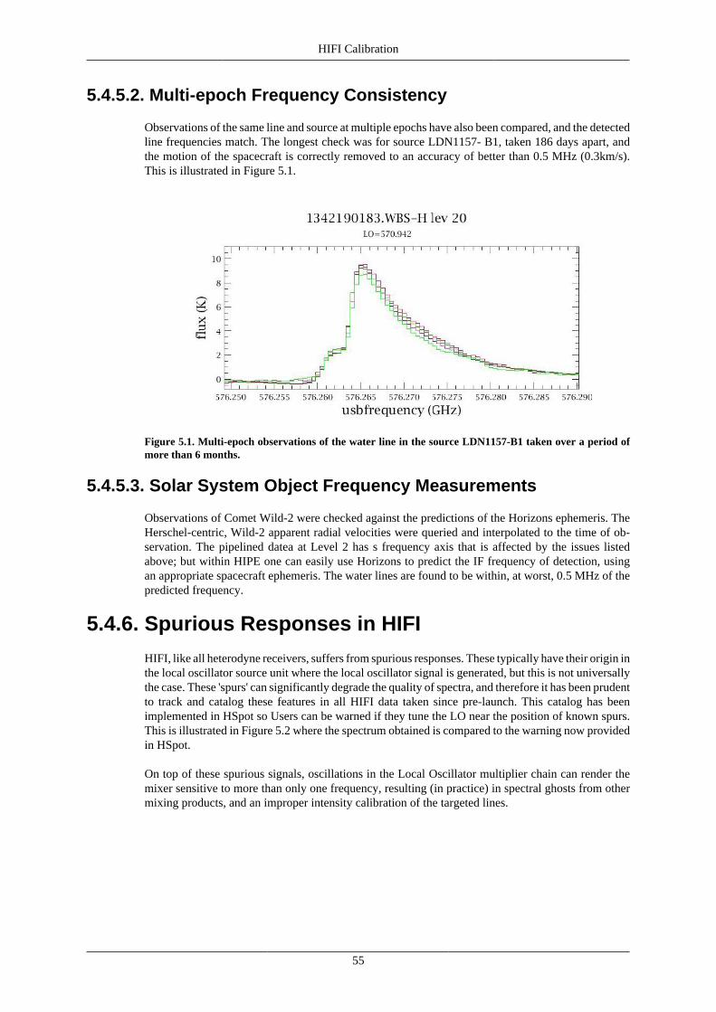
HIFI Calibration
55
5.4.5.2. Multi-epoch Frequency Consistency
Observations of the same line and source at multiple epochs have also been compared, and the detectedline frequencies match. The longest check was for source LDN1157- B1, taken 186 days apart, andthe motion of the spacecraft is correctly removed to an accuracy of better than 0.5 MHz (0.3km/s).This is illustrated in Figure 5.1.
Figure 5.1. Multi-epoch observations of the water line in the source LDN1157-B1 taken over a period ofmore than 6 months.
5.4.5.3. Solar System Object Frequency Measurements
Observations of Comet Wild-2 were checked against the predictions of the Horizons ephemeris. TheHerschel-centric, Wild-2 apparent radial velocities were queried and interpolated to the time of ob-servation. The pipelined datea at Level 2 has s frequency axis that is affected by the issues listedabove; but within HIPE one can easily use Horizons to predict the IF frequency of detection, usingan appropriate spacecraft ephemeris. The water lines are found to be within, at worst, 0.5 MHz of thepredicted frequency.
5.4.6. Spurious Responses in HIFI
HIFI, like all heterodyne receivers, suffers from spurious responses. These typically have their origin inthe local oscillator source unit where the local oscillator signal is generated, but this is not universallythe case. These 'spurs' can significantly degrade the quality of spectra, and therefore it has been prudentto track and catalog these features in all HIFI data taken since pre-launch. This catalog has beenimplemented in HSpot so Users can be warned if they tune the LO near the position of known spurs.This is illustrated in Figure 5.2 where the spectrum obtained is compared to the warning now providedin HSpot.
On top of these spurious signals, oscillations in the Local Oscillator multiplier chain can render themixer sensitive to more than only one frequency, resulting (in practice) in spectral ghosts from othermixing products, and an improper intensity calibration of the targeted lines.
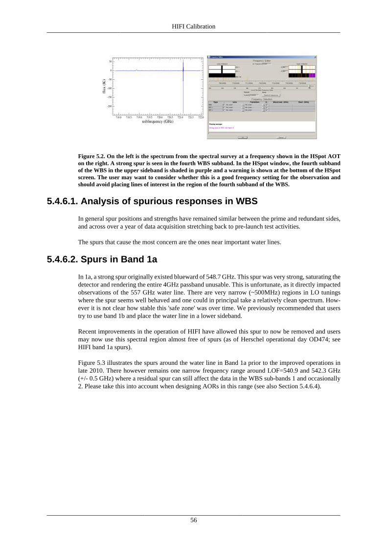
HIFI Calibration
56
Figure 5.2. On the left is the spectrum from the spectral survey at a frequency shown in the HSpot AOTon the right. A strong spur is seen in the fourth WBS subband. In the HSpot window, the fourth subbandof the WBS in the upper sideband is shaded in purple and a warning is shown at the bottom of the HSpotscreen. The user may want to consider whether this is a good frequency setting for the observation andshould avoid placing lines of interest in the region of the fourth subband of the WBS.
5.4.6.1. Analysis of spurious responses in WBS
In general spur positions and strengths have remained similar between the prime and redundant sides,and across over a year of data acquisition stretching back to pre-launch test activities.
The spurs that cause the most concern are the ones near important water lines.
5.4.6.2. Spurs in Band 1a
In 1a, a strong spur originally existed blueward of 548.7 GHz. This spur was very strong, saturating thedetector and rendering the entire 4GHz passband unusable. This is unfortunate, as it directly impactedobservations of the 557 GHz water line. There are very narrow (~500MHz) regions in LO tuningswhere the spur seems well behaved and one could in principal take a relatively clean spectrum. How-ever it is not clear how stable this 'safe zone' was over time. We previously recommended that userstry to use band 1b and place the water line in a lower sideband.
Recent improvements in the operation of HIFI have allowed this spur to now be removed and usersmay now use this spectral region almost free of spurs (as of Herschel operational day OD474; seeHIFI band 1a spurs).
Figure 5.3 illustrates the spurs around the water line in Band 1a prior to the improved operations inlate 2010. There however remains one narrow frequency range around LOF=540.9 and 542.3 GHz(+/- 0.5 GHz) where a residual spur can still affect the data in the WBS sub-bands 1 and occasionally2. Please take this into account when designing AORs in this range (see also Section 5.4.6.4).
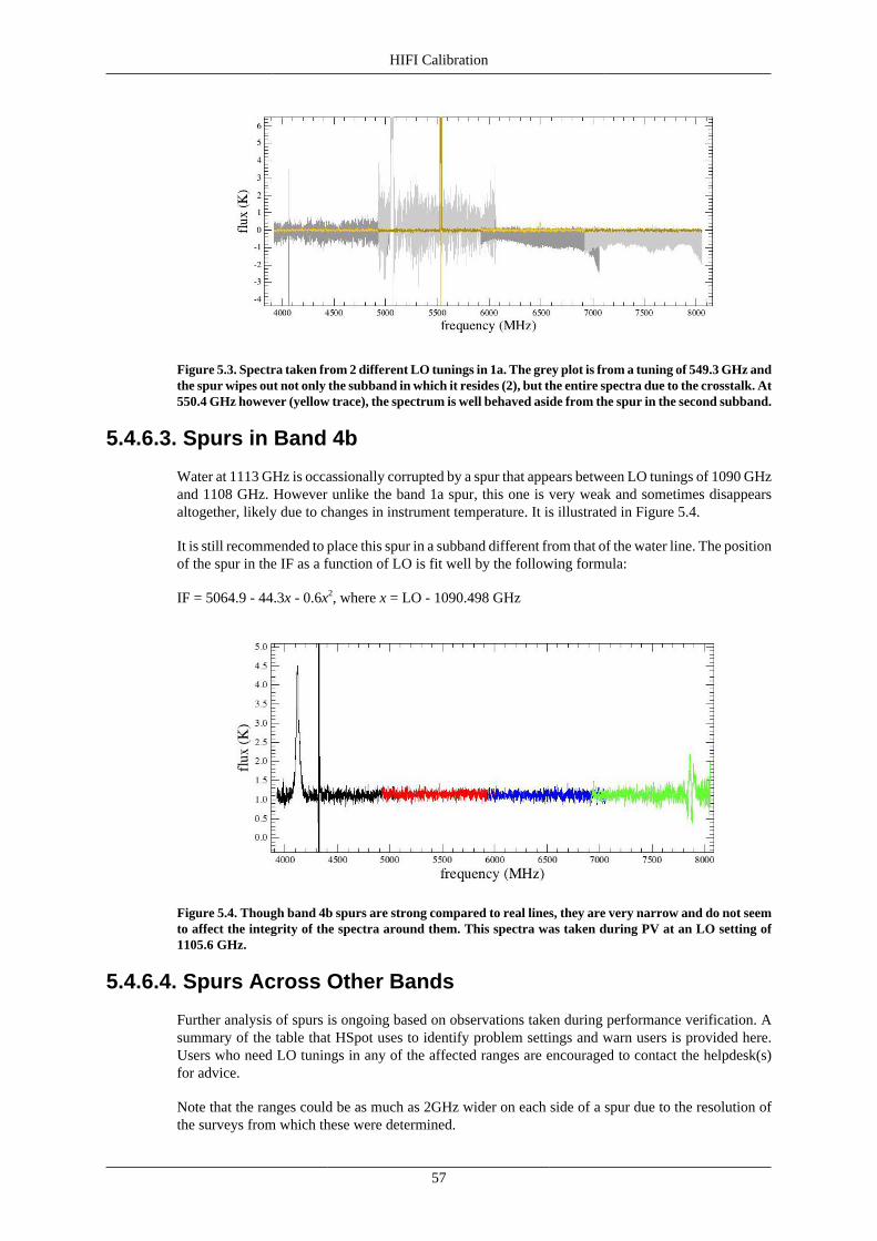
HIFI Calibration
57
Figure 5.3. Spectra taken from 2 different LO tunings in 1a. The grey plot is from a tuning of 549.3 GHz andthe spur wipes out not only the subband in which it resides (2), but the entire spectra due to the crosstalk. At550.4 GHz however (yellow trace), the spectrum is well behaved aside from the spur in the second subband.
5.4.6.3. Spurs in Band 4b
Water at 1113 GHz is occassionally corrupted by a spur that appears between LO tunings of 1090 GHzand 1108 GHz. However unlike the band 1a spur, this one is very weak and sometimes disappearsaltogether, likely due to changes in instrument temperature. It is illustrated in Figure 5.4.
It is still recommended to place this spur in a subband different from that of the water line. The positionof the spur in the IF as a function of LO is fit well by the following formula:
IF = 5064.9 - 44.3x - 0.6x2, where x = LO - 1090.498 GHz
Figure 5.4. Though band 4b spurs are strong compared to real lines, they are very narrow and do not seemto affect the integrity of the spectra around them. This spectra was taken during PV at an LO setting of1105.6 GHz.
5.4.6.4. Spurs Across Other Bands
Further analysis of spurs is ongoing based on observations taken during performance verification. Asummary of the table that HSpot uses to identify problem settings and warn users is provided here.Users who need LO tunings in any of the affected ranges are encouraged to contact the helpdesk(s)for advice.
Note that the ranges could be as much as 2GHz wider on each side of a spur due to the resolution ofthe surveys from which these were determined.
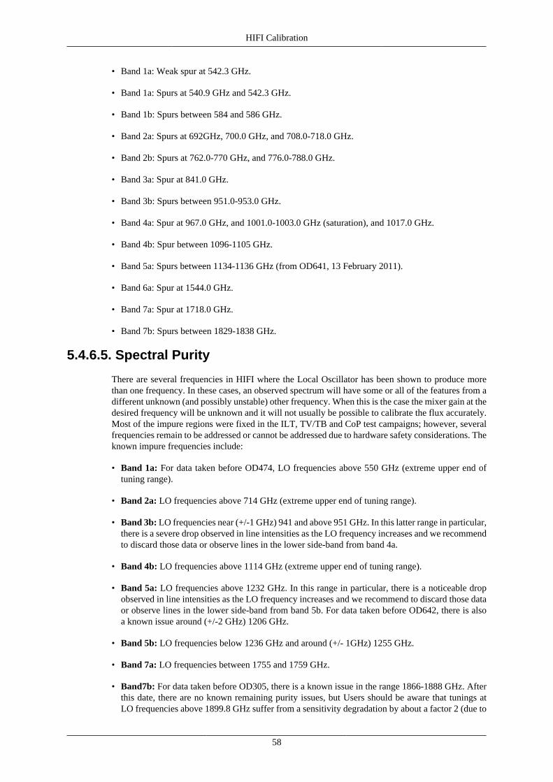
HIFI Calibration
58
• Band 1a: Weak spur at 542.3 GHz.
• Band 1a: Spurs at 540.9 GHz and 542.3 GHz.
• Band 1b: Spurs between 584 and 586 GHz.
• Band 2a: Spurs at 692GHz, 700.0 GHz, and 708.0-718.0 GHz.
• Band 2b: Spurs at 762.0-770 GHz, and 776.0-788.0 GHz.
• Band 3a: Spur at 841.0 GHz.
• Band 3b: Spurs between 951.0-953.0 GHz.
• Band 4a: Spur at 967.0 GHz, and 1001.0-1003.0 GHz (saturation), and 1017.0 GHz.
• Band 4b: Spur between 1096-1105 GHz.
• Band 5a: Spurs between 1134-1136 GHz (from OD641, 13 February 2011).
• Band 6a: Spur at 1544.0 GHz.
• Band 7a: Spur at 1718.0 GHz.
• Band 7b: Spurs between 1829-1838 GHz.
5.4.6.5. Spectral Purity
There are several frequencies in HIFI where the Local Oscillator has been shown to produce morethan one frequency. In these cases, an observed spectrum will have some or all of the features from adifferent unknown (and possibly unstable) other frequency. When this is the case the mixer gain at thedesired frequency will be unknown and it will not usually be possible to calibrate the flux accurately.Most of the impure regions were fixed in the ILT, TV/TB and CoP test campaigns; however, severalfrequencies remain to be addressed or cannot be addressed due to hardware safety considerations. Theknown impure frequencies include:
• Band 1a: For data taken before OD474, LO frequencies above 550 GHz (extreme upper end oftuning range).
• Band 2a: LO frequencies above 714 GHz (extreme upper end of tuning range).
• Band 3b: LO frequencies near (+/-1 GHz) 941 and above 951 GHz. In this latter range in particular,there is a severe drop observed in line intensities as the LO frequency increases and we recommendto discard those data or observe lines in the lower side-band from band 4a.
• Band 4b: LO frequencies above 1114 GHz (extreme upper end of tuning range).
• Band 5a: LO frequencies above 1232 GHz. In this range in particular, there is a noticeable dropobserved in line intensities as the LO frequency increases and we recommend to discard those dataor observe lines in the lower side-band from band 5b. For data taken before OD642, there is alsoa known issue around (+/-2 GHz) 1206 GHz.
• Band 5b: LO frequencies below 1236 GHz and around (+/- 1GHz) 1255 GHz.
• Band 7a: LO frequencies between 1755 and 1759 GHz.
• Band7b: For data taken before OD305, there is a known issue in the range 1866-1888 GHz. Afterthis date, there are no known remaining purity issues, but Users should be aware that tunings atLO frequencies above 1899.8 GHz suffer from a sensitivity degradation by about a factor 2 (due to
HIFI Calibration
59
unavoidable mixer over-pumping). For most sources, this should be far enough for tunings targetingthe [CII] line, where robust tuning is now achieved in most cases. Users should however be awarethat the tuning success in the upper end of band 7b can be influenced by the chain thermalizationhistory, and the exact targeted LO frequency. So there could still be observations that will not benefitfrom the best sensitivity, usually rendering the scientific data very difficult to exploit.
The scheduling implications are summarized as follows:
• Spectral Scans in Bands 3b, 4b and 5a may be carried out as is, and users should inspect and possiblydiscard the spectra taken at the unruly LO frequencies. This will imply some noise degradation afterthe spectrum deconvolution.
• For Spectral Scans in Band 7a, the User is advised to split the frequency coverage into at least twoAORs which avoid the impure areas. As a consequence there will be a slight penalty due to the slewtime tax charged at each AOR, and the (temporary) degradation of the achieved noise at the edgesof the deconvolved spectra due to a coarser redundancy. Once the LO purity has been satisfactorilyestablished, the excluded regions can be scanned if needed. Presently this means that LO tuningsonly over the following ranges are advised: Band 7a: [1701.2 - 1755] and [1759 - 1793.8] GHz .[Note: Several SDP and PSP1 AORs in Band 7a were carried out over these impure ranges, priorto this information being available].
• For observations in Band 7b requesting LO frequencies > 1899.8 GHz, there are currently noscheduling restrictions, but Users must be aware of the lower performances that can result from thetuning issues described above.
• For single frequencies (in AORs using the Point and Map AOTs) whenever possible, the main linesof interest should be moved into the image bands if the new LO frequency falls in an area notaffected by purity issues. Otherwise, it is probably wise to put the observations on hold until thechain is fixed in the targeted frequency area. [Note: this will not have been possible for the veryearly SDP and PSP1 AORs which were scheduled before this information was available].
5.4.6.6. Spurious response in the HRS
Spurs in WBS do not correspond to spurs in HRS. While the investigation of HRS spurs has not yetbeen as detailed as in WBS, it is already clear that the spur in band 1a for instance does not impact theHRS at all. Because spurs are found generally in spectral surveys, and since spectral surveys generallydo not have HRS data, a full catalog of HRS spurs has been slower to generate.
5.4.6.7. Treating Spurs in Software
Spurs are automatically flagged during pipeline processing, and ignored in subsequent processing. Formoderate spurs, this is generally sufficient. Strong spurs however, which corrupt entire subbands orspectra, require an extra step of cleaning.
This is easy to do in software, and we have had excellent success in cleaning up spectral scans foruse by the deconvolution routine.
5.5. The Spatial Response Calibration of HIFI:The framework for the spatial response description of Herschel/HIFI is given in [11]. This documentpresents the terminology related to the topic, and estimates the telescope efficiencies and observationsneeded to assess some of the spatial response parameters.
5.5.1. Context:The intensity calibration approach described in the previous section, involving the measurement ofthe instrument bandpass on hot and cold internal loads, this translates the backend counts to so-called
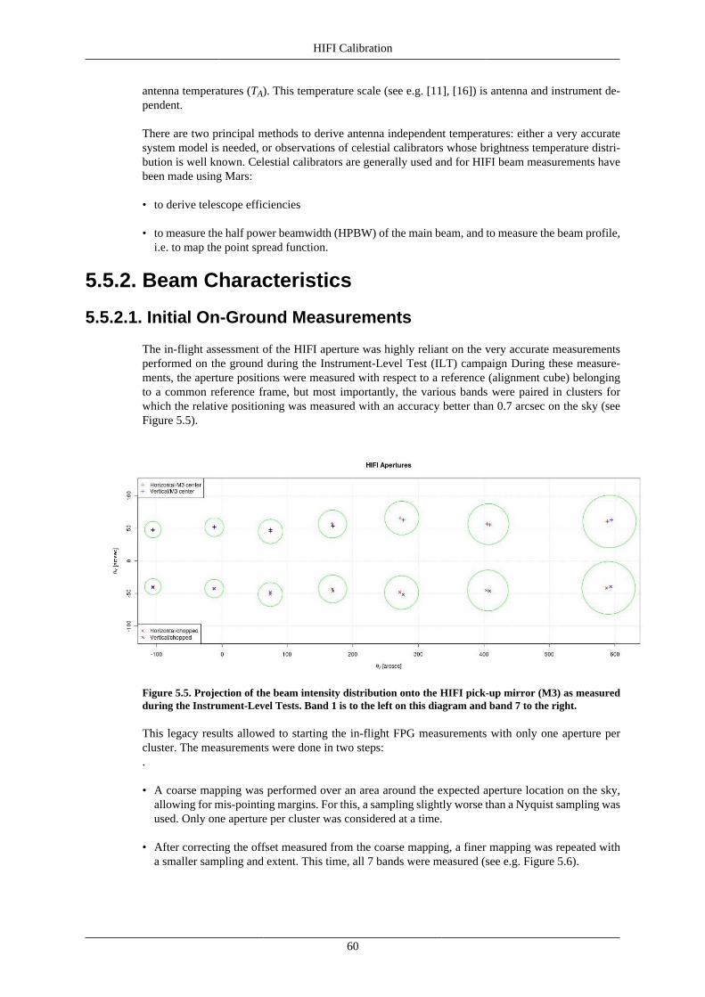
HIFI Calibration
60
antenna temperatures (TA). This temperature scale (see e.g. [11], [16]) is antenna and instrument de-pendent.
There are two principal methods to derive antenna independent temperatures: either a very accuratesystem model is needed, or observations of celestial calibrators whose brightness temperature distri-bution is well known. Celestial calibrators are generally used and for HIFI beam measurements havebeen made using Mars:
• to derive telescope efficiencies
• to measure the half power beamwidth (HPBW) of the main beam, and to measure the beam profile,i.e. to map the point spread function.
5.5.2. Beam Characteristics
5.5.2.1. Initial On-Ground Measurements
The in-flight assessment of the HIFI aperture was highly reliant on the very accurate measurementsperformed on the ground during the Instrument-Level Test (ILT) campaign During these measure-ments, the aperture positions were measured with respect to a reference (alignment cube) belongingto a common reference frame, but most importantly, the various bands were paired in clusters forwhich the relative positioning was measured with an accuracy better than 0.7 arcsec on the sky (seeFigure 5.5).
Figure 5.5. Projection of the beam intensity distribution onto the HIFI pick-up mirror (M3) as measuredduring the Instrument-Level Tests. Band 1 is to the left on this diagram and band 7 to the right.
This legacy results allowed to starting the in-flight FPG measurements with only one aperture percluster. The measurements were done in two steps:.
• A coarse mapping was performed over an area around the expected aperture location on the sky,allowing for mis-pointing margins. For this, a sampling slightly worse than a Nyquist sampling wasused. Only one aperture per cluster was considered at a time.
• After correcting the offset measured from the coarse mapping, a finer mapping was repeated witha smaller sampling and extent. This time, all 7 bands were measured (see e.g. Figure 5.6).
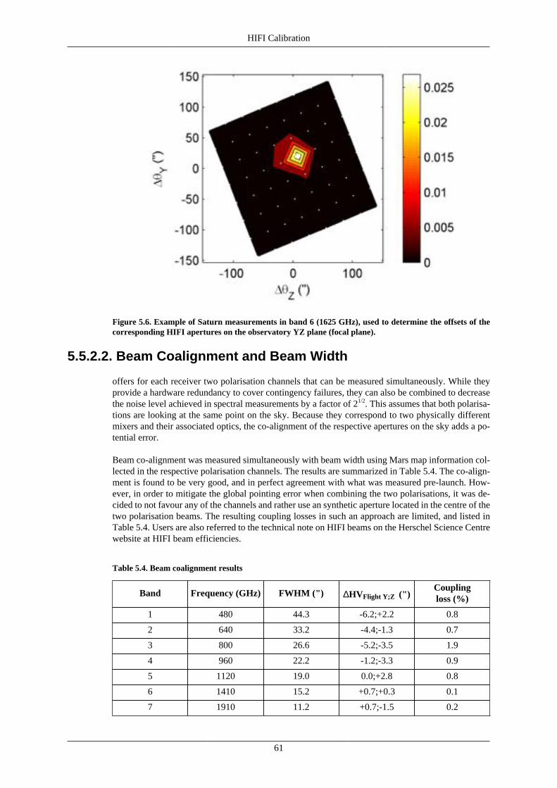
HIFI Calibration
61
Figure 5.6. Example of Saturn measurements in band 6 (1625 GHz), used to determine the offsets of thecorresponding HIFI apertures on the observatory YZ plane (focal plane).
5.5.2.2. Beam Coalignment and Beam Width
offers for each receiver two polarisation channels that can be measured simultaneously. While theyprovide a hardware redundancy to cover contingency failures, they can also be combined to decreasethe noise level achieved in spectral measurements by a factor of 21/2. This assumes that both polarisa-tions are looking at the same point on the sky. Because they correspond to two physically differentmixers and their associated optics, the co-alignment of the respective apertures on the sky adds a po-tential error.
Beam co-alignment was measured simultaneously with beam width using Mars map information col-lected in the respective polarisation channels. The results are summarized in Table 5.4. The co-align-ment is found to be very good, and in perfect agreement with what was measured pre-launch. How-ever, in order to mitigate the global pointing error when combining the two polarisations, it was de-cided to not favour any of the channels and rather use an synthetic aperture located in the centre of thetwo polarisation beams. The resulting coupling losses in such an approach are limited, and listed inTable 5.4. Users are also referred to the technical note on HIFI beams on the Herschel Science Centrewebsite at HIFI beam efficiencies.
Table 5.4. Beam coalignment results
Band Frequency (GHz) FWHM (") ∆HVFlight Y;Z (")Couplingloss (%)
1 480 44.3 -6.2;+2.2 0.8
2 640 33.2 -4.4;-1.3 0.7
3 800 26.6 -5.2;-3.5 1.9
4 960 22.2 -1.2;-3.3 0.9
5 1120 19.0 0.0;+2.8 0.8
6 1410 15.2 +0.7;+0.3 0.1
7 1910 11.2 +0.7;-1.5 0.2
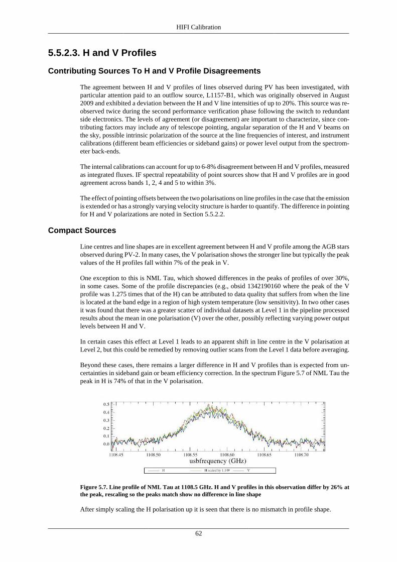
HIFI Calibration
62
5.5.2.3. H and V Profiles
Contributing Sources To H and V Profile Disagreements
The agreement between H and V profiles of lines observed during PV has been investigated, withparticular attention paid to an outflow source, L1157-B1, which was originally observed in August2009 and exhibited a deviation between the H and V line intensities of up to 20%. This source was re-observed twice during the second performance verification phase following the switch to redundantside electronics. The levels of agreement (or disagreement) are important to characterize, since con-tributing factors may include any of telescope pointing, angular separation of the H and V beams onthe sky, possible intrinsic polarization of the source at the line frequencies of interest, and instrumentcalibrations (different beam efficiencies or sideband gains) or power level output from the spectrom-eter back-ends.
The internal calibrations can account for up to 6-8% disagreement between H and V profiles, measuredas integrated fluxes. IF spectral repeatability of point sources show that H and V profiles are in goodagreement across bands 1, 2, 4 and 5 to within 3%.
The effect of pointing offsets between the two polarisations on line profiles in the case that the emissionis extended or has a strongly varying velocity structure is harder to quantify. The difference in pointingfor H and V polarizations are noted in Section 5.5.2.2.
Compact Sources
Line centres and line shapes are in excellent agreement between H and V profile among the AGB starsobserved during PV-2. In many cases, the V polarisation shows the stronger line but typically the peakvalues of the H profiles fall within 7% of the peak in V.
One exception to this is NML Tau, which showed differences in the peaks of profiles of over 30%,in some cases. Some of the profile discrepancies (e.g., obsid 1342190160 where the peak of the Vprofile was 1.275 times that of the H) can be attributed to data quality that suffers from when the lineis located at the band edge in a region of high system temperature (low sensitivity). In two other casesit was found that there was a greater scatter of individual datasets at Level 1 in the pipeline processedresults about the mean in one polarisation (V) over the other, possibly reflecting varying power outputlevels between H and V.
In certain cases this effect at Level 1 leads to an apparent shift in line centre in the V polarisation atLevel 2, but this could be remedied by removing outlier scans from the Level 1 data before averaging.
Beyond these cases, there remains a larger difference in H and V profiles than is expected from un-certainties in sideband gain or beam efficiency correction. In the spectrum Figure 5.7 of NML Tau thepeak in H is 74% of that in the V polarisation.
Figure 5.7. Line profile of NML Tau at 1108.5 GHz. H and V profiles in this observation differ by 26% atthe peak, rescaling so the peaks match show no difference in line shape
After simply scaling the H polarisation up it is seen that there is no mismatch in profile shape.
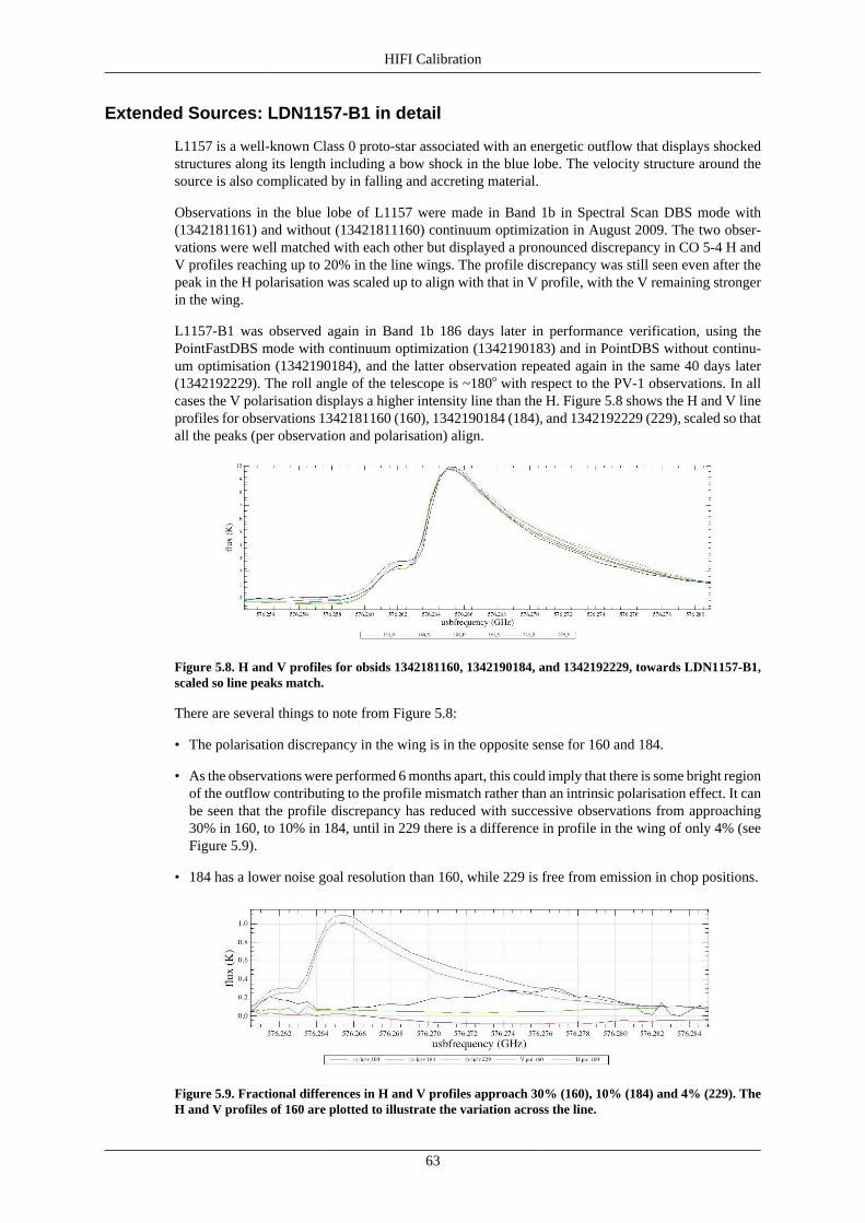
HIFI Calibration
63
Extended Sources: LDN1157-B1 in detail
L1157 is a well-known Class 0 proto-star associated with an energetic outflow that displays shockedstructures along its length including a bow shock in the blue lobe. The velocity structure around thesource is also complicated by in falling and accreting material.
Observations in the blue lobe of L1157 were made in Band 1b in Spectral Scan DBS mode with(1342181161) and without (13421811160) continuum optimization in August 2009. The two obser-vations were well matched with each other but displayed a pronounced discrepancy in CO 5-4 H andV profiles reaching up to 20% in the line wings. The profile discrepancy was still seen even after thepeak in the H polarisation was scaled up to align with that in V profile, with the V remaining strongerin the wing.
L1157-B1 was observed again in Band 1b 186 days later in performance verification, using thePointFastDBS mode with continuum optimization (1342190183) and in PointDBS without continu-um optimisation (1342190184), and the latter observation repeated again in the same 40 days later(1342192229). The roll angle of the telescope is ~180o with respect to the PV-1 observations. In allcases the V polarisation displays a higher intensity line than the H. Figure 5.8 shows the H and V lineprofiles for observations 1342181160 (160), 1342190184 (184), and 1342192229 (229), scaled so thatall the peaks (per observation and polarisation) align.
Figure 5.8. H and V profiles for obsids 1342181160, 1342190184, and 1342192229, towards LDN1157-B1,scaled so line peaks match.
There are several things to note from Figure 5.8:
• The polarisation discrepancy in the wing is in the opposite sense for 160 and 184.
• As the observations were performed 6 months apart, this could imply that there is some bright regionof the outflow contributing to the profile mismatch rather than an intrinsic polarisation effect. It canbe seen that the profile discrepancy has reduced with successive observations from approaching30% in 160, to 10% in 184, until in 229 there is a difference in profile in the wing of only 4% (seeFigure 5.9).
• 184 has a lower noise goal resolution than 160, while 229 is free from emission in chop positions.
Figure 5.9. Fractional differences in H and V profiles approach 30% (160), 10% (184) and 4% (229). TheH and V profiles of 160 are plotted to illustrate the variation across the line.
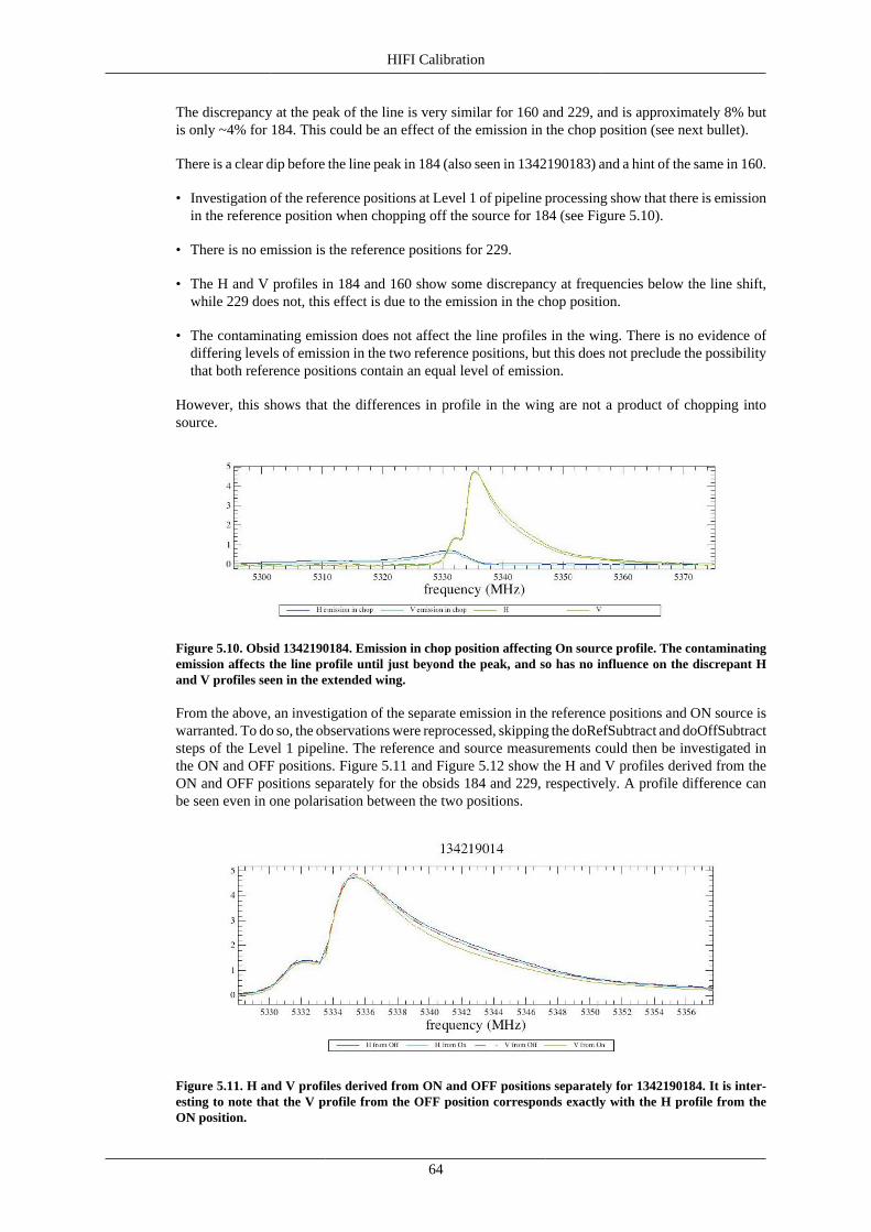
HIFI Calibration
64
The discrepancy at the peak of the line is very similar for 160 and 229, and is approximately 8% butis only ~4% for 184. This could be an effect of the emission in the chop position (see next bullet).
There is a clear dip before the line peak in 184 (also seen in 1342190183) and a hint of the same in 160.
• Investigation of the reference positions at Level 1 of pipeline processing show that there is emissionin the reference position when chopping off the source for 184 (see Figure 5.10).
• There is no emission is the reference positions for 229.
• The H and V profiles in 184 and 160 show some discrepancy at frequencies below the line shift,while 229 does not, this effect is due to the emission in the chop position.
• The contaminating emission does not affect the line profiles in the wing. There is no evidence ofdiffering levels of emission in the two reference positions, but this does not preclude the possibilitythat both reference positions contain an equal level of emission.
However, this shows that the differences in profile in the wing are not a product of chopping intosource.
Figure 5.10. Obsid 1342190184. Emission in chop position affecting On source profile. The contaminatingemission affects the line profile until just beyond the peak, and so has no influence on the discrepant Hand V profiles seen in the extended wing.
From the above, an investigation of the separate emission in the reference positions and ON source iswarranted. To do so, the observations were reprocessed, skipping the doRefSubtract and doOffSubtractsteps of the Level 1 pipeline. The reference and source measurements could then be investigated inthe ON and OFF positions. Figure 5.11 and Figure 5.12 show the H and V profiles derived from theON and OFF positions separately for the obsids 184 and 229, respectively. A profile difference canbe seen even in one polarisation between the two positions.
Figure 5.11. H and V profiles derived from ON and OFF positions separately for 1342190184. It is inter-esting to note that the V profile from the OFF position corresponds exactly with the H profile from theON position.
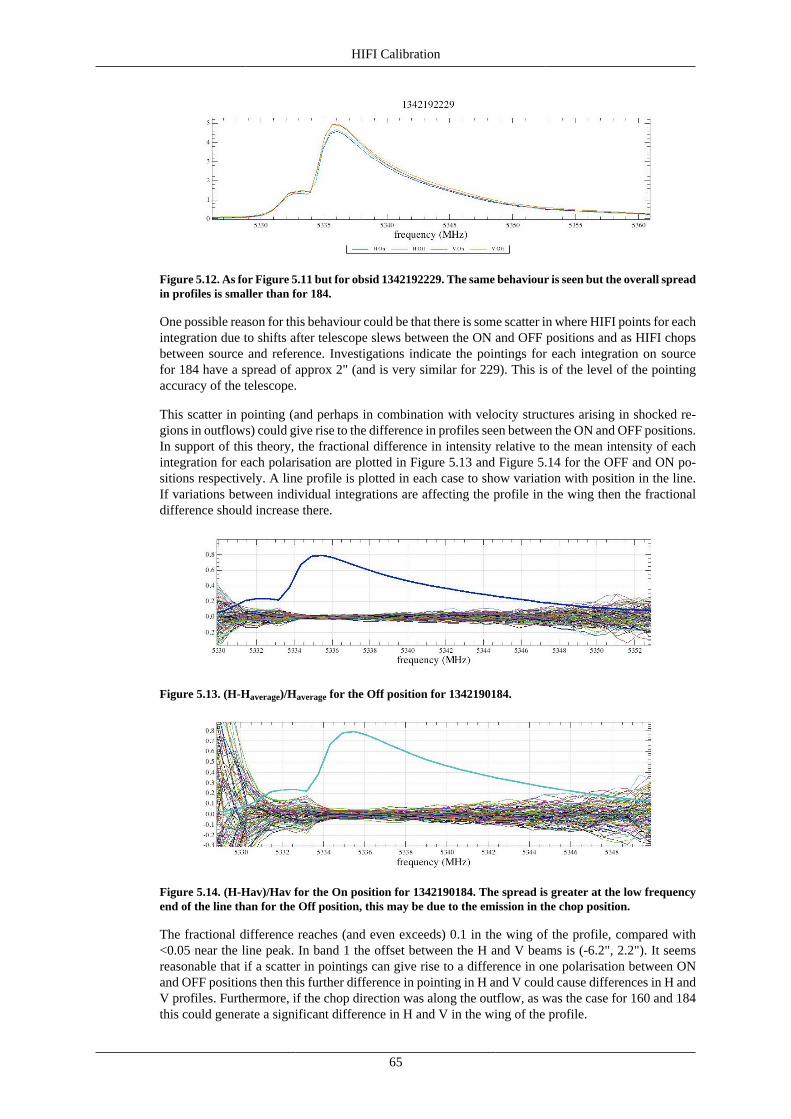
HIFI Calibration
65
Figure 5.12. As for Figure 5.11 but for obsid 1342192229. The same behaviour is seen but the overall spreadin profiles is smaller than for 184.
One possible reason for this behaviour could be that there is some scatter in where HIFI points for eachintegration due to shifts after telescope slews between the ON and OFF positions and as HIFI chopsbetween source and reference. Investigations indicate the pointings for each integration on sourcefor 184 have a spread of approx 2" (and is very similar for 229). This is of the level of the pointingaccuracy of the telescope.
This scatter in pointing (and perhaps in combination with velocity structures arising in shocked re-gions in outflows) could give rise to the difference in profiles seen between the ON and OFF positions.In support of this theory, the fractional difference in intensity relative to the mean intensity of eachintegration for each polarisation are plotted in Figure 5.13 and Figure 5.14 for the OFF and ON po-sitions respectively. A line profile is plotted in each case to show variation with position in the line.If variations between individual integrations are affecting the profile in the wing then the fractionaldifference should increase there.
Figure 5.13. (H-Haverage)/Haverage for the Off position for 1342190184.
Figure 5.14. (H-Hav)/Hav for the On position for 1342190184. The spread is greater at the low frequencyend of the line than for the Off position, this may be due to the emission in the chop position.
The fractional difference reaches (and even exceeds) 0.1 in the wing of the profile, compared with<0.05 near the line peak. In band 1 the offset between the H and V beams is (-6.2", 2.2"). It seemsreasonable that if a scatter in pointings can give rise to a difference in one polarisation between ONand OFF positions then this further difference in pointing in H and V could cause differences in H andV profiles. Furthermore, if the chop direction was along the outflow, as was the case for 160 and 184this could generate a significant difference in H and V in the wing of the profile.
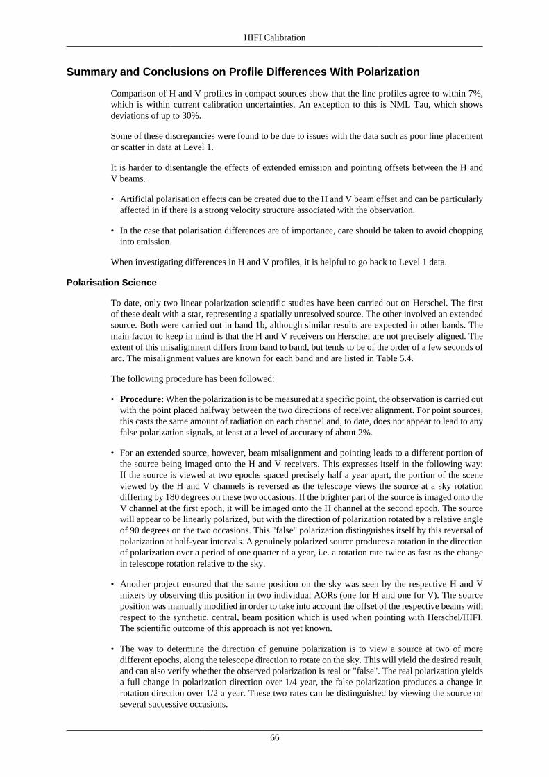
HIFI Calibration
66
Summary and Conclusions on Profile Differences With Polarization
Comparison of H and V profiles in compact sources show that the line profiles agree to within 7%,which is within current calibration uncertainties. An exception to this is NML Tau, which showsdeviations of up to 30%.
Some of these discrepancies were found to be due to issues with the data such as poor line placementor scatter in data at Level 1.
It is harder to disentangle the effects of extended emission and pointing offsets between the H andV beams.
• Artificial polarisation effects can be created due to the H and V beam offset and can be particularlyaffected in if there is a strong velocity structure associated with the observation.
• In the case that polarisation differences are of importance, care should be taken to avoid choppinginto emission.
When investigating differences in H and V profiles, it is helpful to go back to Level 1 data.
Polarisation Science
To date, only two linear polarization scientific studies have been carried out on Herschel. The firstof these dealt with a star, representing a spatially unresolved source. The other involved an extendedsource. Both were carried out in band 1b, although similar results are expected in other bands. Themain factor to keep in mind is that the H and V receivers on Herschel are not precisely aligned. Theextent of this misalignment differs from band to band, but tends to be of the order of a few seconds ofarc. The misalignment values are known for each band and are listed in Table 5.4.
The following procedure has been followed:
• Procedure: When the polarization is to be measured at a specific point, the observation is carried outwith the point placed halfway between the two directions of receiver alignment. For point sources,this casts the same amount of radiation on each channel and, to date, does not appear to lead to anyfalse polarization signals, at least at a level of accuracy of about 2%.
• For an extended source, however, beam misalignment and pointing leads to a different portion ofthe source being imaged onto the H and V receivers. This expresses itself in the following way:If the source is viewed at two epochs spaced precisely half a year apart, the portion of the sceneviewed by the H and V channels is reversed as the telescope views the source at a sky rotationdiffering by 180 degrees on these two occasions. If the brighter part of the source is imaged onto theV channel at the first epoch, it will be imaged onto the H channel at the second epoch. The sourcewill appear to be linearly polarized, but with the direction of polarization rotated by a relative angleof 90 degrees on the two occasions. This "false" polarization distinguishes itself by this reversal ofpolarization at half-year intervals. A genuinely polarized source produces a rotation in the directionof polarization over a period of one quarter of a year, i.e. a rotation rate twice as fast as the changein telescope rotation relative to the sky.
• Another project ensured that the same position on the sky was seen by the respective H and Vmixers by observing this position in two individual AORs (one for H and one for V). The sourceposition was manually modified in order to take into account the offset of the respective beams withrespect to the synthetic, central, beam position which is used when pointing with Herschel/HIFI.The scientific outcome of this approach is not yet known.
• The way to determine the direction of genuine polarization is to view a source at two of moredifferent epochs, along the telescope direction to rotate on the sky. This will yield the desired result,and can also verify whether the observed polarization is real or "false". The real polarization yieldsa full change in polarization direction over 1/4 year, the false polarization produces a change inrotation direction over 1/2 a year. These two rates can be distinguished by viewing the source onseveral successive occasions.
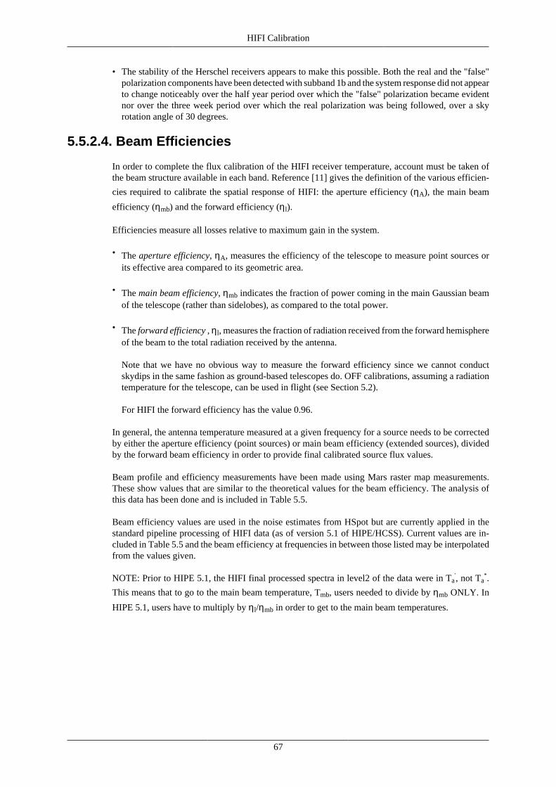
HIFI Calibration
67
• The stability of the Herschel receivers appears to make this possible. Both the real and the "false"polarization components have been detected with subband 1b and the system response did not appearto change noticeably over the half year period over which the "false" polarization became evidentnor over the three week period over which the real polarization was being followed, over a skyrotation angle of 30 degrees.
5.5.2.4. Beam Efficiencies
In order to complete the flux calibration of the HIFI receiver temperature, account must be taken ofthe beam structure available in each band. Reference [11] gives the definition of the various efficien-
cies required to calibrate the spatial response of HIFI: the aperture efficiency (ηA), the main beam
efficiency (ηmb) and the forward efficiency (ηl).
Efficiencies measure all losses relative to maximum gain in the system.
• The aperture efficiency, ηA, measures the efficiency of the telescope to measure point sources orits effective area compared to its geometric area.
• The main beam efficiency, ηmb indicates the fraction of power coming in the main Gaussian beamof the telescope (rather than sidelobes), as compared to the total power.
• The forward efficiency , ηl, measures the fraction of radiation received from the forward hemisphereof the beam to the total radiation received by the antenna.
Note that we have no obvious way to measure the forward efficiency since we cannot conductskydips in the same fashion as ground-based telescopes do. OFF calibrations, assuming a radiationtemperature for the telescope, can be used in flight (see Section 5.2).
For HIFI the forward efficiency has the value 0.96.
In general, the antenna temperature measured at a given frequency for a source needs to be correctedby either the aperture efficiency (point sources) or main beam efficiency (extended sources), dividedby the forward beam efficiency in order to provide final calibrated source flux values.
Beam profile and efficiency measurements have been made using Mars raster map measurements.These show values that are similar to the theoretical values for the beam efficiency. The analysis ofthis data has been done and is included in Table 5.5.
Beam efficiency values are used in the noise estimates from HSpot but are currently applied in thestandard pipeline processing of HIFI data (as of version 5.1 of HIPE/HCSS). Current values are in-cluded in Table 5.5 and the beam efficiency at frequencies in between those listed may be interpolatedfrom the values given.
NOTE: Prior to HIPE 5.1, the HIFI final processed spectra in level2 of the data were in Ta', not Ta
*.
This means that to go to the main beam temperature, Tmb, users needed to divide by ηmb ONLY. In
HIPE 5.1, users have to multiply by ηl/ηmb in order to get to the main beam temperatures.
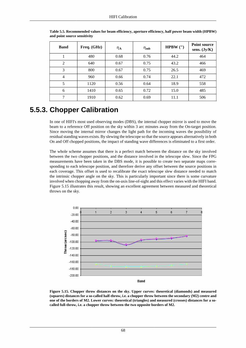
HIFI Calibration
68
Table 5.5. Recommended values for beam efficiency, aperture efficiency, half power beam width (HPBW)and point source sensitivity
Band Freq. (GHz) ηA ηmb HPBW (")Point sourcesens. (Jy/K)
1 480 0.68 0.76 44.2 464
2 640 0.67 0.75 43.2 466
3 800 0.67 0.75 26.5 469
4 960 0.66 0.74 22.1 472
5 1120 0.56 0.64 18.9 558
6 1410 0.65 0.72 15.0 485
7 1910 0.62 0.69 11.1 506
5.5.3. Chopper Calibration
In one of HIFI's most used observing modes (DBS), the internal chopper mirror is used to move thebeam to a reference Off position on the sky within 3 arc minutes away from the On-target position.Since moving the internal mirror changes the light path for the incoming waves the possibility ofresidual standing waves exists. By slewing the telescope so that the source appears alternatively in bothOn and Off chopped positions, the impact of standing wave differences is eliminated to a first order.
The whole scheme assumes that there is a perfect match between the distance on the sky involvedbetween the two chopper positions, and the distance involved in the telescope slew. Since the FPGmeasurements have been taken in the DBS mode, it is possible to create two separate maps corre-sponding to each telescope position, and therefore derive any offset between the source positions ineach coverage. This offset is used to recalibrate the exact telescope slew distance needed to matchthe intrinsic chopper angle on the sky. This is particularly important since there is some curvatureinvolved when chopping away from the on-axis line-of-sight and this effect varies with the HIFI band.Figure 5.15 illustrates this result, showing an excellent agreement between measured and theoreticalthrows on the sky.
Figure 5.15. Chopper throw distances on the sky. Upper curves: theoretical (diamonds) and measured(squares) distances for a so-called half-throw, i.e. a chopper throw between the secondary (M2) centre andone of the borders of M2. Lower curves: theoretical (triangles) and measured (crosses) distances for a so-called full-throw, i.e. a chopper throw between the two opposite borders of M2.
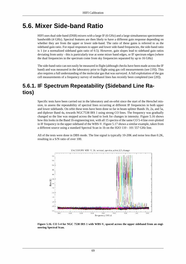
HIFI Calibration
69
5.6. Mixer Side-band RatioHIFI uses dual side-band (DSB) mixers with a large IF (6 GHz) and a large simultaneous spectrometerbandwidth (4 GHz). Spectral features are then likely to have a different gain response depending onwhether they are from the upper or lower side-band. The ratio of these gains is referred to as thesideband gain ratio. For equal responses to upper and lower side-band frequencies, the side-band ratiois 1 (or a normalized sideband gain ratio of 0.5). However, gain slopes lead to sideband gain ratiosdeviating from unity - this is particularly true at some mixer band edges, or IF spectrum edges (wherethe dual frequencies in the spectrum come from sky frequencies separated by up to 16 GHz)
The side-band ratio can not easily be measured in flight (although checks have been made across the IFband) and was measured in the laboratory prior to flight using gas cell measurements (see [19]). Thisalso requires a full understanding of the molecular gas that was surveyed. A full exploitation of the gascell measurements of a frequency survey of methanol lines has recently been completed (see [20]).
5.6.1. IF Spectrum Repeatability (Sideband Line Ra-tios)
Specific tests have been carried out in the laboratory and on-orbit since the start of the Herschel mis-sion, to assess the repeatability of spectral lines occurring at different IF frequencies in both upperand lower sidebands. On orbit these tests have been done so far in beam splitter Bands 1b, 2a, and 5a,and diplexer Band 4a, towards NGC7538 IRS 1 using strong CO lines. The frequency was graduallychanged so the line was stepped across the band to look for changes in intensity. Figure 5.16 showshow this looks in the Band 1b engineering test, with all 15 spectra of the same CO 5-4 line over-plottedin IF frequency in the upper sideband of the WBS-V. Figure 5.17 shows a similar example, taken froma different source using a standard Spectral Scan in 1b on the H2O 110 - 101 557 GHz line.
All of the tests were done in DBS mode. The line signal is typically 10-20K and noise less than 0.2K,resulting in a S/N ratio of over 100.
Figure 5.16. CO 5-4 for NGC 7538 IRS 1 with WBS-V, spaced across the upper sideband from an engi-neering Spectral Scan.
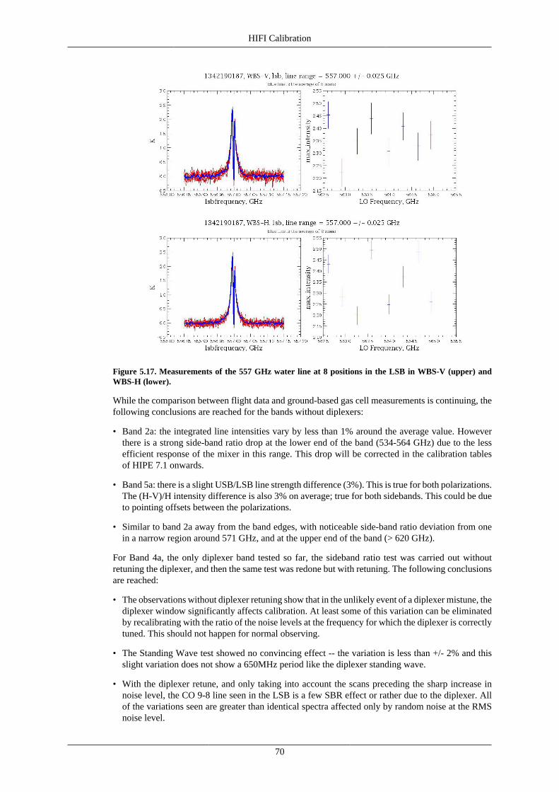
HIFI Calibration
70
Figure 5.17. Measurements of the 557 GHz water line at 8 positions in the LSB in WBS-V (upper) andWBS-H (lower).
While the comparison between flight data and ground-based gas cell measurements is continuing, thefollowing conclusions are reached for the bands without diplexers:
• Band 2a: the integrated line intensities vary by less than 1% around the average value. Howeverthere is a strong side-band ratio drop at the lower end of the band (534-564 GHz) due to the lessefficient response of the mixer in this range. This drop will be corrected in the calibration tablesof HIPE 7.1 onwards.
• Band 5a: there is a slight USB/LSB line strength difference (3%). This is true for both polarizations.The (H-V)/H intensity difference is also 3% on average; true for both sidebands. This could be dueto pointing offsets between the polarizations.
• Similar to band 2a away from the band edges, with noticeable side-band ratio deviation from onein a narrow region around 571 GHz, and at the upper end of the band (> 620 GHz).
For Band 4a, the only diplexer band tested so far, the sideband ratio test was carried out withoutretuning the diplexer, and then the same test was redone but with retuning. The following conclusionsare reached:
• The observations without diplexer retuning show that in the unlikely event of a diplexer mistune, thediplexer window significantly affects calibration. At least some of this variation can be eliminatedby recalibrating with the ratio of the noise levels at the frequency for which the diplexer is correctlytuned. This should not happen for normal observing.
• The Standing Wave test showed no convincing effect -- the variation is less than +/- 2% and thisslight variation does not show a 650MHz period like the diplexer standing wave.
• With the diplexer retune, and only taking into account the scans preceding the sharp increase innoise level, the CO 9-8 line seen in the LSB is a few SBR effect or rather due to the diplexer. Allof the variations seen are greater than identical spectra affected only by random noise at the RMSnoise level.
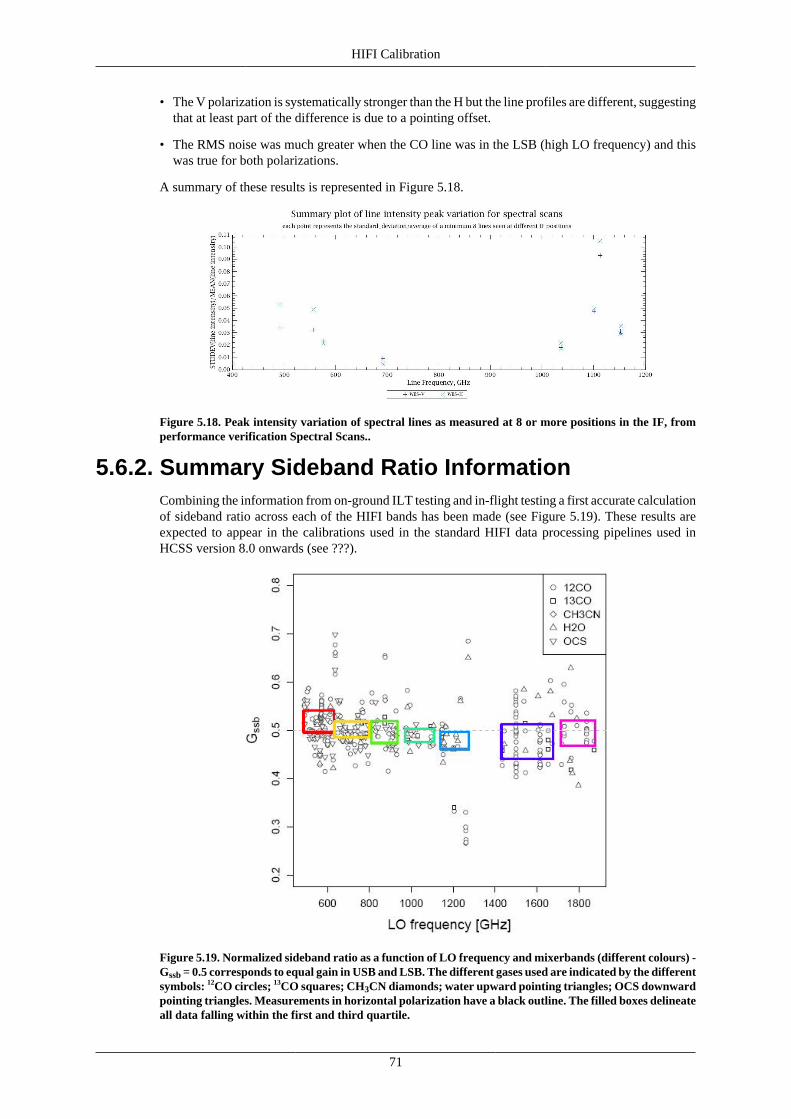
HIFI Calibration
71
• The V polarization is systematically stronger than the H but the line profiles are different, suggestingthat at least part of the difference is due to a pointing offset.
• The RMS noise was much greater when the CO line was in the LSB (high LO frequency) and thiswas true for both polarizations.
A summary of these results is represented in Figure 5.18.
Figure 5.18. Peak intensity variation of spectral lines as measured at 8 or more positions in the IF, fromperformance verification Spectral Scans..
5.6.2. Summary Sideband Ratio InformationCombining the information from on-ground ILT testing and in-flight testing a first accurate calculationof sideband ratio across each of the HIFI bands has been made (see Figure 5.19). These results areexpected to appear in the calibrations used in the standard HIFI data processing pipelines used inHCSS version 8.0 onwards (see ???).
Figure 5.19. Normalized sideband ratio as a function of LO frequency and mixerbands (different colours) -Gssb = 0.5 corresponds to equal gain in USB and LSB. The different gases used are indicated by the differentsymbols: 12CO circles; 13CO squares; CH3CN diamonds; water upward pointing triangles; OCS downwardpointing triangles. Measurements in horizontal polarization have a black outline. The filled boxes delineateall data falling within the first and third quartile.
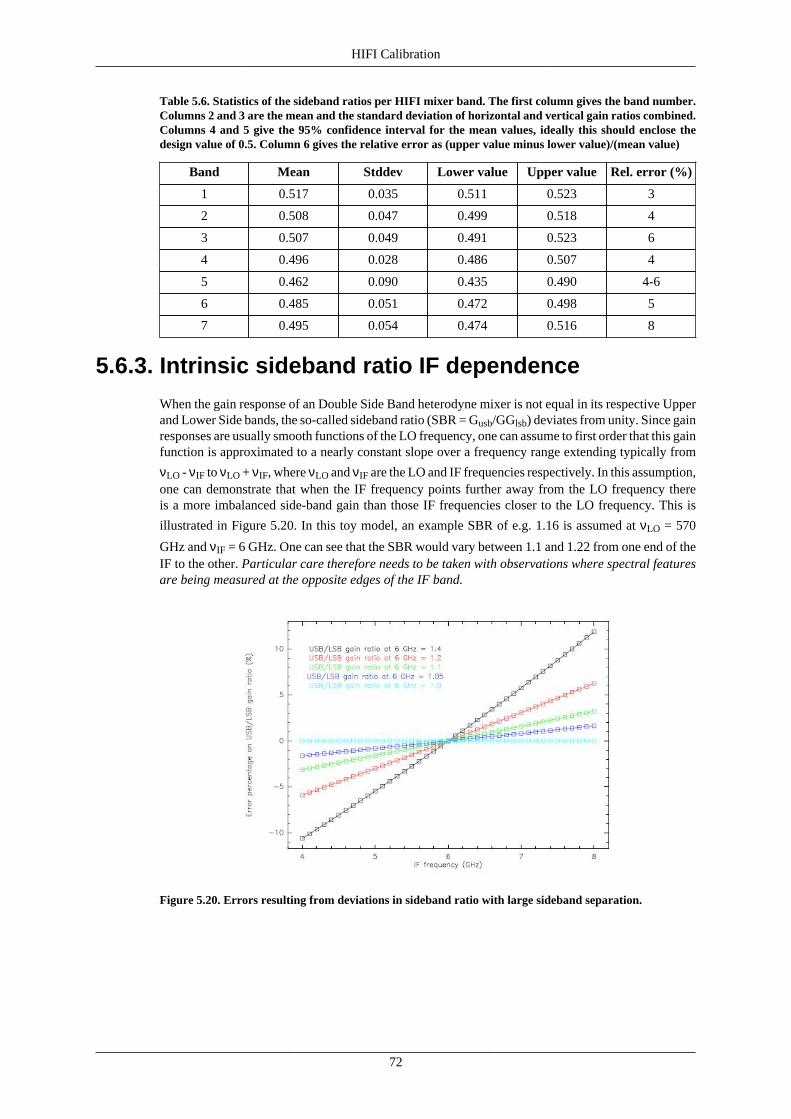
HIFI Calibration
72
Table 5.6. Statistics of the sideband ratios per HIFI mixer band. The first column gives the band number.Columns 2 and 3 are the mean and the standard deviation of horizontal and vertical gain ratios combined.Columns 4 and 5 give the 95% confidence interval for the mean values, ideally this should enclose thedesign value of 0.5. Column 6 gives the relative error as (upper value minus lower value)/(mean value)
Band Mean Stddev Lower value Upper value Rel. error (%)
1 0.517 0.035 0.511 0.523 3
2 0.508 0.047 0.499 0.518 4
3 0.507 0.049 0.491 0.523 6
4 0.496 0.028 0.486 0.507 4
5 0.462 0.090 0.435 0.490 4-6
6 0.485 0.051 0.472 0.498 5
7 0.495 0.054 0.474 0.516 8
5.6.3. Intrinsic sideband ratio IF dependence
When the gain response of an Double Side Band heterodyne mixer is not equal in its respective Upperand Lower Side bands, the so-called sideband ratio (SBR = Gusb/GGlsb) deviates from unity. Since gainresponses are usually smooth functions of the LO frequency, one can assume to first order that this gainfunction is approximated to a nearly constant slope over a frequency range extending typically from
νLO - νIF to νLO + νIF, where νLO and νIF are the LO and IF frequencies respectively. In this assumption,one can demonstrate that when the IF frequency points further away from the LO frequency thereis a more imbalanced side-band gain than those IF frequencies closer to the LO frequency. This is
illustrated in Figure 5.20. In this toy model, an example SBR of e.g. 1.16 is assumed at νLO = 570
GHz and νIF = 6 GHz. One can see that the SBR would vary between 1.1 and 1.22 from one end of theIF to the other. Particular care therefore needs to be taken with observations where spectral featuresare being measured at the opposite edges of the IF band.
Figure 5.20. Errors resulting from deviations in sideband ratio with large sideband separation.
HIFI Calibration
73
5.7. Summary: overall calibration of HIFI anderror budget:
5.7.1. Strategy summary:The absolute intensity calibration is being derived from planetary observations (most especially Mars),via the measurement of the telescope efficiencies. Once the efficiencies are known, and assuming theydo not change significantly with time, internal loads can be used as the day-to-day stable reference forintensity calibration (transfer function). Differencing measurements for calibration sources are doneboth ON source (source-reference) and on an OFF position (off-reference). It is the double differenceof these two modulated spectra that finally offers a correction of the baseline ripples (standing waves).
5.7.2. Error budgetThe error budget indicates the total error for the HIFI calibration. It is dependent on the band (maybethe frequency), on the observing mode and on the source observed. The budget includes both frequencyand intensity calibration. It also takes into account the uncertainty on the telescope pointing and theeffects of optical standing waves (Opt. standing waves) in each of the HIFI bands.
There are two types of error considered:
• Systematic Errors: are described within the calibration framework (e.g. temperature sensor on hotand cold loads). We presume multiple measurements will not improve these errors. There are twoways to combine these error: linearly (pessimistic) or quadratically (uncorrelated errors). The errorbudget for systematic errors are contained in Table 5.7. Note that line non-linearity has been foundto be a negligible error.
• random errors: the normal radiometric errors which are statistical in nature. Multiple observationswill reduce these errors. The cost is time.
Table 5.7. Overall error budget. The following table provides the percentage flux error associated witheach component of the error budget.
Error source Band 1/2 Band 3/4 Band 5 Band 6/7
Sideband ratio 3-4 4-6 4-6 5-8
Hot load coupling <1 <1 <1 <1
Cold load coupling <1 <1 <1 <1
Hot load temperature <1 <1 <1 <1
Cold load temperature <1 <1 <1 <1
Planetary model error1 <3 <3 <3 <3
Beam Efficiency <5 <5 <10 <5
Pointing <1 <2 <2 <4
Opt. standing waves 4 4 3 3
74
Chapter 6. Using HSpot to CreateHIFI Observations
6.1. OverviewWithin HSpot we have four modes of taking point sources (Dual Beam Switch (DBS) -- with fast orslow chop, load chop -- with or without a reference OFF position, frequency switch -- with or withouta reference OFF position, and position switch), three modes of mapping ("On-the-fly" -- or scan --mapping with an OFF or frequency switch reference, and raster mapping using DBS).
Under mapping modes there is also the possibility of a fixed position 5-point cross designed to handlesmall pointing or position inaccuracies to provide accurate flux measuremetns.
There is also a special mode for allowing large spectral coverage in a single observation -- the spectralscan mode, which can use either a dual beam switch or frequency switch reference scheme.
It is also possible to set up the HIFI spectrometers so that multiple resolutions are available coveringseveral spectral lines in a single observation.
In this chapter we provide examples of how to set up some simple, and not so simple, observations thatcover point sources, mapping and spectral scans. The intent of this chapter is to illustrate the generalway in which to formulate HIFI AORs that are suitable for submission to the Herschel Science Centre(HSC) as part of a proposal. Along the way a number of the features of the HSpot observation planningsoftware will be illustrated.
6.2. HSpot Components for Setting Up a HIFIObservation
6.2.1. Working with A HIFI Pointed or Mapping Obser-vation Template
In order to set up an observing request in HSpot, we start by working with an AOT (AstronomicalObserving Template). Such a template leads you through the possible choices for setting up HIFI sothat the final request (an Astronomical Observing Request -- AOR) contains all the necessary infor-mation for the correct frequencies to be measured on the sky by each of the spectrometers (and theirsubbands) that are being used.
There are three types of AOTs.
• HIFI Pointed Observation
• HIFI Mapping Observation
• HIFI Spectral Scan
The HIFI Pointed and Mapping Observation setups have several similarities (except for the observingmode choices) while the spectral scan mode is a special mode that allows for large frequency rangecoverage within a single observation.
To choose one of the three AOTs, go to the "Observation" pulldown menu at the top of the main screenthat appears when HSpot is started up (see Figure 6.1).
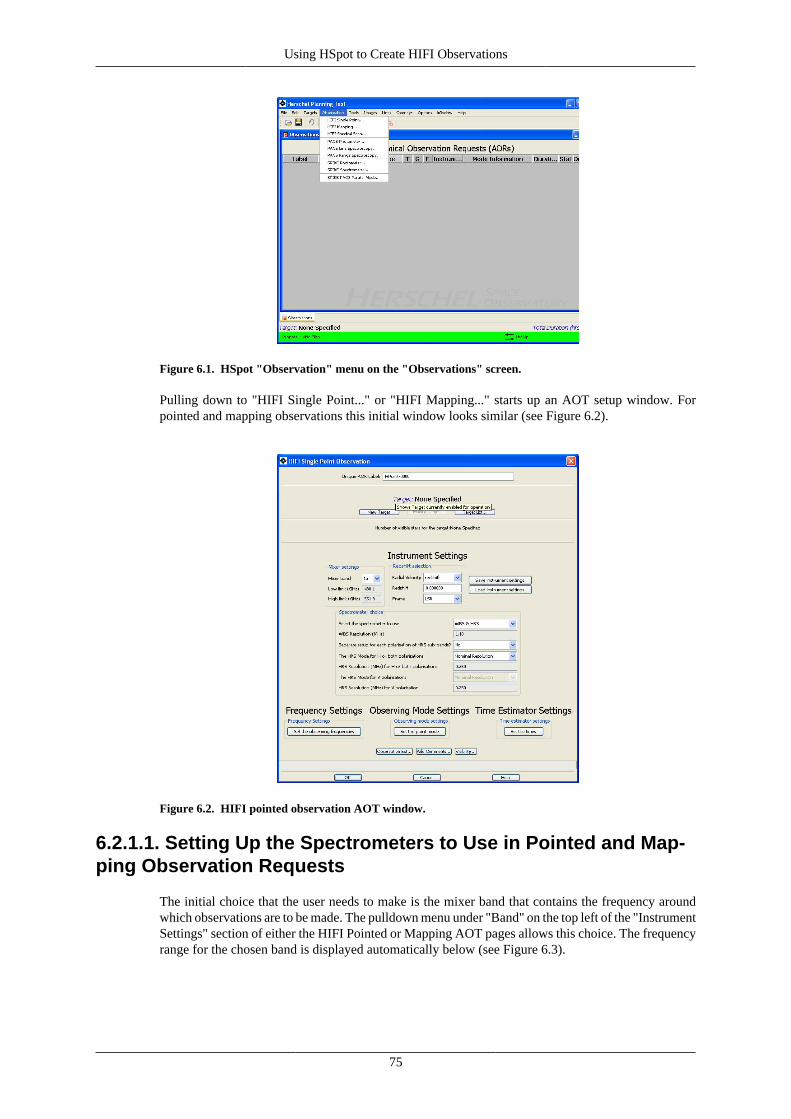
Using HSpot to Create HIFI Observations
75
Figure 6.1. HSpot "Observation" menu on the "Observations" screen.
Pulling down to "HIFI Single Point..." or "HIFI Mapping..." starts up an AOT setup window. Forpointed and mapping observations this initial window looks similar (see Figure 6.2).
Figure 6.2. HIFI pointed observation AOT window.
6.2.1.1. Setting Up the Spectrometers to Use in Pointed and Map-ping Observation Requests
The initial choice that the user needs to make is the mixer band that contains the frequency aroundwhich observations are to be made. The pulldown menu under "Band" on the top left of the "InstrumentSettings" section of either the HIFI Pointed or Mapping AOT pages allows this choice. The frequencyrange for the chosen band is displayed automatically below (see Figure 6.3).
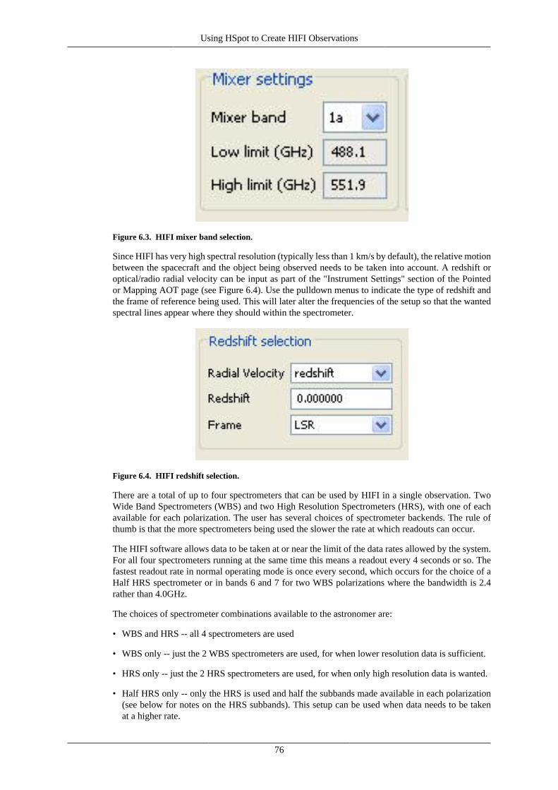
Using HSpot to Create HIFI Observations
76
Figure 6.3. HIFI mixer band selection.
Since HIFI has very high spectral resolution (typically less than 1 km/s by default), the relative motionbetween the spacecraft and the object being observed needs to be taken into account. A redshift oroptical/radio radial velocity can be input as part of the "Instrument Settings" section of the Pointedor Mapping AOT page (see Figure 6.4). Use the pulldown menus to indicate the type of redshift andthe frame of reference being used. This will later alter the frequencies of the setup so that the wantedspectral lines appear where they should within the spectrometer.
Figure 6.4. HIFI redshift selection.
There are a total of up to four spectrometers that can be used by HIFI in a single observation. TwoWide Band Spectrometers (WBS) and two High Resolution Spectrometers (HRS), with one of eachavailable for each polarization. The user has several choices of spectrometer backends. The rule ofthumb is that the more spectrometers being used the slower the rate at which readouts can occur.
The HIFI software allows data to be taken at or near the limit of the data rates allowed by the system.For all four spectrometers running at the same time this means a readout every 4 seconds or so. Thefastest readout rate in normal operating mode is once every second, which occurs for the choice of aHalf HRS spectrometer or in bands 6 and 7 for two WBS polarizations where the bandwidth is 2.4rather than 4.0GHz.
The choices of spectrometer combinations available to the astronomer are:
• WBS and HRS -- all 4 spectrometers are used
• WBS only -- just the 2 WBS spectrometers are used, for when lower resolution data is sufficient.
• HRS only -- just the 2 HRS spectrometers are used, for when only high resolution data is wanted.
• Half HRS only -- only the HRS is used and half the subbands made available in each polarization(see below for notes on the HRS subbands). This setup can be used when data needs to be takenat a higher rate.
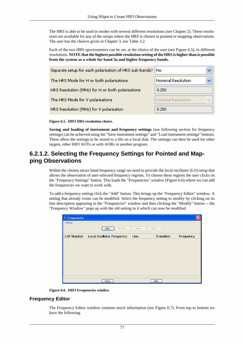
Using HSpot to Create HIFI Observations
77
The HRS is able to be used in modes with several different resolutions (see Chapter 2). These resolu-tions are available for any of the setups where the HRS is chosen in pointed or mapping observations.The user has the choices given in Chapter 3, see Table 3.2.
Each of the two HRS spectrometers can be set, at the choice of the user (see Figure 6.5), to differentresolutions. NOTE that the highest possible resolution setting of the HRS is higher than is possiblefrom the system as a whole for band 3a and higher frequency bands.
Figure 6.5. HIFI HRS resolution choice.
Saving and loading of instrument and frequency settings (see following section for frequencysettings) can be achieved using the "Save instrument settings" and "Load instrument settings" buttons.These allow the settings to be stored to a file on a local disk. The settings can then be used for othertargets, other HIFI AOTs or with AORs in another program.
6.2.1.2. Selecting the Frequency Settings for Pointed and Map-ping Observations
Within the chosen mixer band frequency range we need to provide the local oscillator (LO) setup thatallows the observation of user-selected frequency regions. To choose these regions the user clicks onthe "Frequency Settings" button. This loads the "Frequencies" window (Figure 6.6) where we can addthe frequencies we want to work with.
To add a frequency setting click the "Add" button. This brings up the "Frequency Editor" window. Asetting that already exists can be modified. Select the frequency setting to modify by clicking on itsline description appearing in the "Frequencies" window and then clicking the "Modify" button -- the"Frequency Window" pops up with the old setting in it which can now be modified.
Figure 6.6. HIFI Frequencies window
Frequency Editor
The Frequency Editor window contains much information (see Figure 6.7). From top to bottom wehave the following.
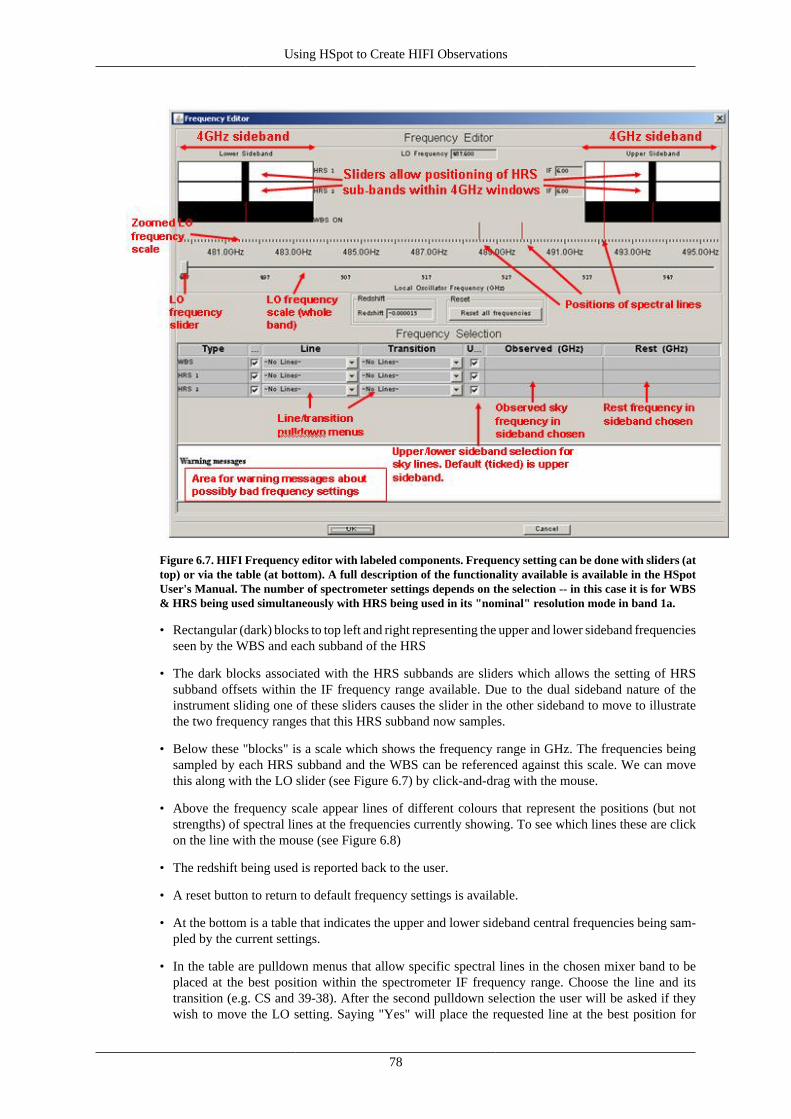
Using HSpot to Create HIFI Observations
78
Figure 6.7. HIFI Frequency editor with labeled components. Frequency setting can be done with sliders (attop) or via the table (at bottom). A full description of the functionality available is available in the HSpotUser's Manual. The number of spectrometer settings depends on the selection -- in this case it is for WBS& HRS being used simultaneously with HRS being used in its "nominal" resolution mode in band 1a.
• Rectangular (dark) blocks to top left and right representing the upper and lower sideband frequenciesseen by the WBS and each subband of the HRS
• The dark blocks associated with the HRS subbands are sliders which allows the setting of HRSsubband offsets within the IF frequency range available. Due to the dual sideband nature of theinstrument sliding one of these sliders causes the slider in the other sideband to move to illustratethe two frequency ranges that this HRS subband now samples.
• Below these "blocks" is a scale which shows the frequency range in GHz. The frequencies beingsampled by each HRS subband and the WBS can be referenced against this scale. We can movethis along with the LO slider (see Figure 6.7) by click-and-drag with the mouse.
• Above the frequency scale appear lines of different colours that represent the positions (but notstrengths) of spectral lines at the frequencies currently showing. To see which lines these are clickon the line with the mouse (see Figure 6.8)
• The redshift being used is reported back to the user.
• A reset button to return to default frequency settings is available.
• At the bottom is a table that indicates the upper and lower sideband central frequencies being sam-pled by the current settings.
• In the table are pulldown menus that allow specific spectral lines in the chosen mixer band to beplaced at the best position within the spectrometer IF frequency range. Choose the line and itstransition (e.g. CS and 39-38). After the second pulldown selection the user will be asked if theywish to move the LO setting. Saying "Yes" will place the requested line at the best position for
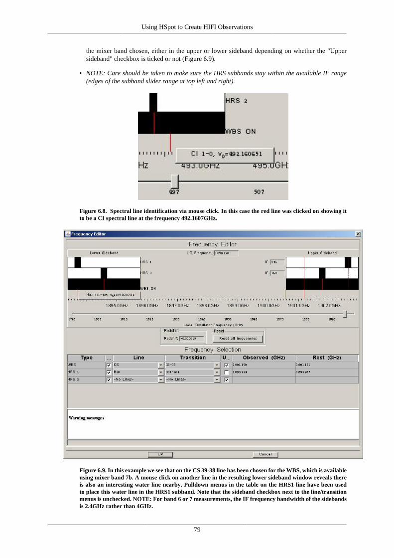
Using HSpot to Create HIFI Observations
79
the mixer band chosen, either in the upper or lower sideband depending on whether the "Uppersideband" checkbox is ticked or not (Figure 6.9).
• NOTE: Care should be taken to make sure the HRS subbands stay within the available IF range(edges of the subband slider range at top left and right).
Figure 6.8. Spectral line identification via mouse click. In this case the red line was clicked on showing itto be a CI spectral line at the frequency 492.1607GHz.
Figure 6.9. In this example we see that on the CS 39-38 line has been chosen for the WBS, which is availableusing mixer band 7b. A mouse click on another line in the resulting lower sideband window reveals thereis also an interesting water line nearby. Pulldown menus in the table on the HRS1 line have been usedto place this water line in the HRS1 subband. Note that the sideband checkbox next to the line/transitionmenus is unchecked. NOTE: For band 6 or 7 measurements, the IF frequency bandwidth of the sidebandsis 2.4GHz rather than 4GHz.
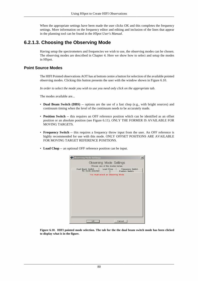
Using HSpot to Create HIFI Observations
80
When the appropriate settings have been made the user clicks OK and this completes the frequencysettings. More information on the frequency editor and editing and inclusion of the lines that appearin the planning tool can be found in the HSpot User's Manual.
6.2.1.3. Choosing the Observing Mode
Having setup the spectrometers and frequencies we wish to use, the observing modes can be chosen.The observing modes are described in Chapter 4. Here we show how to select and setup the modesin HSpot.
Point Source Modes
The HIFI Pointed observations AOT has at bottom centre a button for selection of the available pointedobserving modes. Clicking this button presents the user with the window shown in Figure 6.10.
In order to select the mode you wish to use you need only click on the appropriate tab.
The modes available are...
• Dual Beam Switch (DBS) -- options are the use of a fast chop (e.g., with bright sources) andcontinuum timing when the level of the continuum needs to be accurately made.
• Position Switch -- this requires an OFF reference position which can be identified as an offsetposition or an absolute position (see Figure 6.11). ONLY THE FORMER IS AVAILABLE FORMOVING TARGETS.
• Frequency Switch -- this requires a frequency throw input from the user. An OFF reference ishighly recommended for use with this mode. ONLY OFFSET POSITIONS ARE AVAILABLEFOR MOVING TARGET REFERENCE POSITIONS.
• Load Chop -- an optional OFF reference position can be input.
Figure 6.10. HIFI pointed mode selection. The tab for the the dual beam switch mode has been clickedto display what is in the figure.
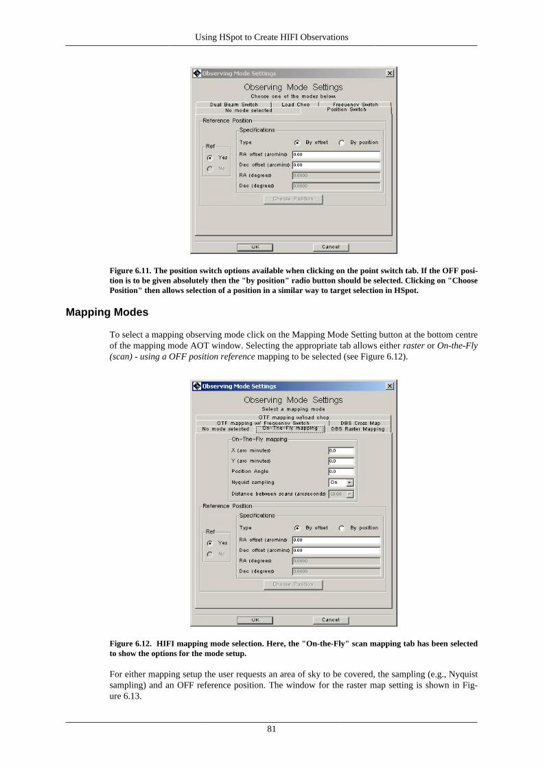
Using HSpot to Create HIFI Observations
81
Figure 6.11. The position switch options available when clicking on the point switch tab. If the OFF posi-tion is to be given absolutely then the "by position" radio button should be selected. Clicking on "ChoosePosition" then allows selection of a position in a similar way to target selection in HSpot.
Mapping Modes
To select a mapping observing mode click on the Mapping Mode Setting button at the bottom centreof the mapping mode AOT window. Selecting the appropriate tab allows either raster or On-the-Fly(scan) - using a OFF position reference mapping to be selected (see Figure 6.12).
Figure 6.12. HIFI mapping mode selection. Here, the "On-the-Fly" scan mapping tab has been selectedto show the options for the mode setup.
For either mapping setup the user requests an area of sky to be covered, the sampling (e.g., Nyquistsampling) and an OFF reference position. The window for the raster map setting is shown in Fig-ure 6.13.
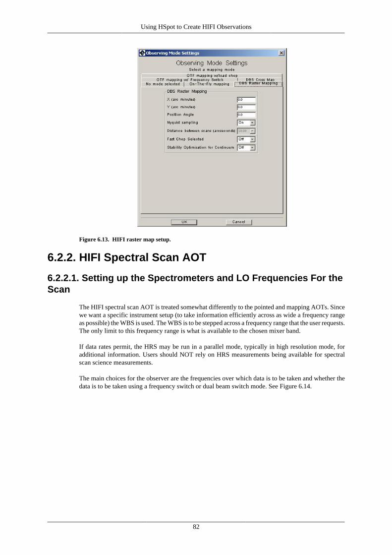
Using HSpot to Create HIFI Observations
82
Figure 6.13. HIFI raster map setup.
6.2.2. HIFI Spectral Scan AOT
6.2.2.1. Setting up the Spectrometers and LO Frequencies For theScan
The HIFI spectral scan AOT is treated somewhat differently to the pointed and mapping AOTs. Sincewe want a specific instrument setup (to take information efficiently across as wide a frequency rangeas possible) the WBS is used. The WBS is to be stepped across a frequency range that the user requests.The only limit to this frequency range is what is available to the chosen mixer band.
If data rates permit, the HRS may be run in a parallel mode, typically in high resolution mode, foradditional information. Users should NOT rely on HRS measurements being available for spectralscan science measurements.
The main choices for the observer are the frequencies over which data is to be taken and whether thedata is to be taken using a frequency switch or dual beam switch mode. See Figure 6.14.
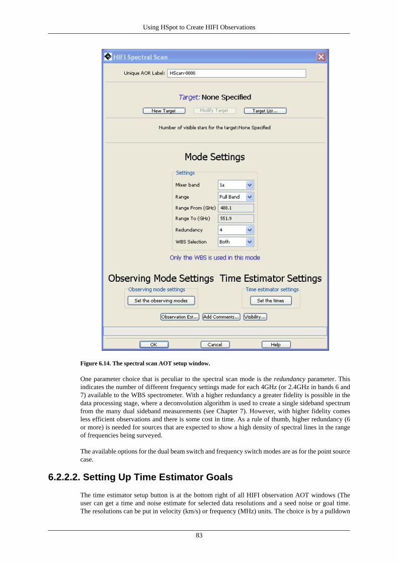
Using HSpot to Create HIFI Observations
83
Figure 6.14. The spectral scan AOT setup window.
One parameter choice that is peculiar to the spectral scan mode is the redundancy parameter. Thisindicates the number of different frequency settings made for each 4GHz (or 2.4GHz in bands 6 and7) available to the WBS spectrometer. With a higher redundancy a greater fidelity is possible in thedata processing stage, where a deconvolution algorithm is used to create a single sideband spectrumfrom the many dual sideband measurements (see Chapter 7). However, with higher fidelity comesless efficient observations and there is some cost in time. As a rule of thumb, higher redundancy (6or more) is needed for sources that are expected to show a high density of spectral lines in the rangeof frequencies being surveyed.
The available options for the dual beam switch and frequency switch modes are as for the point sourcecase.
6.2.2.2. Setting Up Time Estimator Goals
The time estimator setup button is at the bottom right of all HIFI observation AOT windows (Theuser can get a time and noise estimate for selected data resolutions and a seed noise or goal time.The resolutions can be put in velocity (km/s) or frequency (MHz) units. The choice is by a pulldown
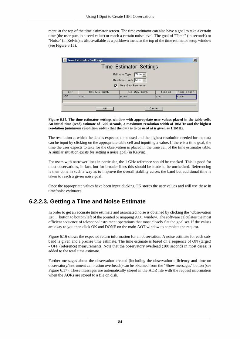
Using HSpot to Create HIFI Observations
84
menu at the top of the time estimator screen. The time estimator can also have a goal to take a certaintime (the user puts in a seed value) or reach a certain noise level. The goal of "Time" (in seconds) or"Noise" (in Kelvin) is also available as a pulldown menu at the top of the time estimator setup window(see Figure 6.15).
Figure 6.15. The time estimator settings window with appropriate user values placed in the table cells.An initial time (seed) estimate of 1200 seconds, a maximum resolution width of 10MHz and the highestresolution (minimum resolution width) that the data is to be used at is given as 1.1MHz.
The resolution at which the data is expected to be used and the highest resolution needed for the datacan be input by clicking on the appropriate table cell and inputting a value. If there is a time goal, thetime the user expects to take for the observation is placed in the time cell of the time estimator table.A similar situation exists for setting a noise goal (in Kelvin).
For users with narrower lines in particular, the 1 GHz reference should be checked. This is good formost observations, in fact, but for broader lines this should be made to be unchecked. Referencingis then done in such a way as to improve the overall stability across the band but additional time istaken to reach a given noise goal.
Once the appropriate values have been input clicking OK stores the user values and will use these intime/noise estimates.
6.2.2.3. Getting a Time and Noise Estimate
In order to get an accurate time estimate and associated noise is obtained by clicking the "ObservationEst..." button to bottom left of the pointed or mapping AOT window. The software calculates the mostefficient sequence of telescope/instrument operations that most closely fits the goal set. If the valuesare okay to you then click OK and DONE on the main AOT window to complete the request.
Figure 6.16 shows the expected return information for an observation. A noise estimate for each sub-band is given and a precise time estimate. The time estimate is based on a sequence of ON (target)- OFF (reference) measurements. Note that the observatory overhead (180 seconds in most cases) isadded to the total time estimate.
Further messages about the observation created (including the observation efficiency and time onobservatory/instrument calibration overheads) can be obtained from the "Show messages" button (seeFigure 6.17). These messages are automatically stored in the AOR file with the request informationwhen the AORs are stored to a file on disk.
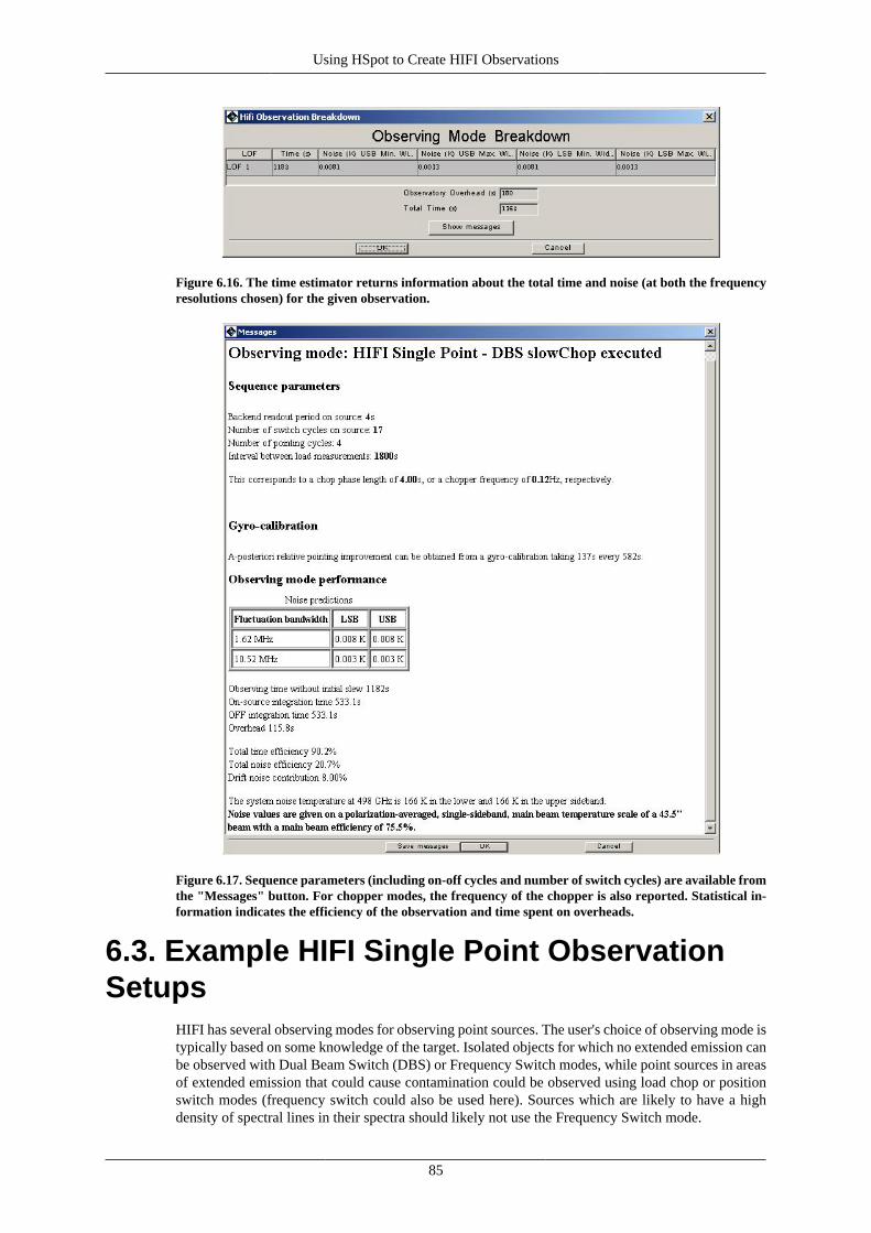
Using HSpot to Create HIFI Observations
85
Figure 6.16. The time estimator returns information about the total time and noise (at both the frequencyresolutions chosen) for the given observation.
Figure 6.17. Sequence parameters (including on-off cycles and number of switch cycles) are available fromthe "Messages" button. For chopper modes, the frequency of the chopper is also reported. Statistical in-formation indicates the efficiency of the observation and time spent on overheads.
6.3. Example HIFI Single Point ObservationSetups
HIFI has several observing modes for observing point sources. The user's choice of observing mode istypically based on some knowledge of the target. Isolated objects for which no extended emission canbe observed with Dual Beam Switch (DBS) or Frequency Switch modes, while point sources in areasof extended emission that could cause contamination could be observed using load chop or positionswitch modes (frequency switch could also be used here). Sources which are likely to have a highdensity of spectral lines in their spectra should likely not use the Frequency Switch mode.
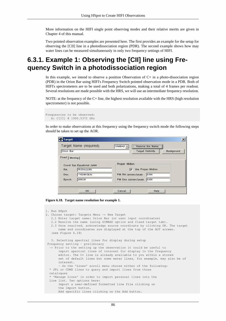
Using HSpot to Create HIFI Observations
86
More information on the HIFI single point observing modes and their relative merits are given inChapter 4 of this manual.
Two pointed observation examples are presented here. The first provides an example for the setup forobserving the [CII] line in a photodissociation region (PDR). The second example shows how maywater lines can be measured simultaneously in only two frequency settings of HIFI.
6.3.1. Example 1: Observing the [CII] line using Fre-quency Switch in a photodissociation region
In this example, we intend to observe a position Observation of C+ in a photo-dissociation region(PDR) in the Orion Bar using HIFI's Frequency Switch pointed observation mode in a PDR. Both ofHIFI's spectrometers are to be used and both polarizations, making a total of 4 frames per readout.Several resolutions are made possible with the HRS, we will use an intermediate frequency resolution.
NOTE: at the frequency of the C+ line, the highest resolution available with the HRS (high resolutionspectrometer) is not possible.
Frequencies to be observed: A: C[II] @ 1900.5372 GHz
In order to make observations at this frequency using the frequency switch mode the following stepsshould be taken to set up the AOR.
Figure 6.18. Target name resolution for example 1.
1. Run HSpot2. Choose target: Targets Menu -> New Target 2.1 Enter target name: Orion Bar (or user input coordinates) 2.2 Resolve the name (using SIMBAD option and fixed target tab). 2.3 Once resolved, acknowledge source coordinate by clicking OK. The target name and coordinates are displayed at the top of the AOT screen. (see Figure 6.18)
3. Selecting spectral lines for display during setup Frequency setting - preliminary -> Prior to the setting up the observation it could be useful to import spectral lines of interest for display in the frequency editor. The C+ line is already available to you within a stored set of default lines but some water lines, for example, may also be of interest. - On the "Lines" scroll menu choose either of the following: * JPL or CDMS lines to query and import lines from those catalogues * "Manage Lines" in order to import personal lines into the line list. Two options here: Import a user-defined formatted line file clicking on the Import button. Add specific lines clicking on the Add button.
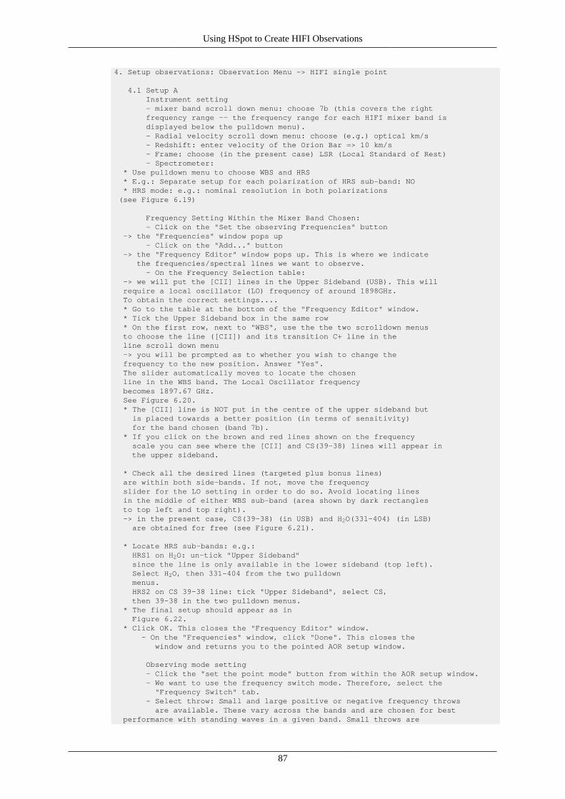
Using HSpot to Create HIFI Observations
87
4. Setup observations: Observation Menu -> HIFI single point
4.1 Setup A Instrument setting - mixer band scroll down menu: choose 7b (this covers the right frequency range -- the frequency range for each HIFI mixer band is displayed below the pulldown menu). - Radial velocity scroll down menu: choose (e.g.) optical km/s - Redshift: enter velocity of the Orion Bar => 10 km/s - Frame: choose (in the present case) LSR (Local Standard of Rest) - Spectrometer: * Use pulldown menu to choose WBS and HRS * E.g.: Separate setup for each polarization of HRS sub-band: NO * HRS mode: e.g.: nominal resolution in both polarizations (see Figure 6.19)
Frequency Setting Within the Mixer Band Chosen: - Click on the "Set the observing Frequencies" button -> the "Frequencies" window pops up - Click on the "Add..." button -> the "Frequency Editor" window pops up. This is where we indicate the frequencies/spectral lines we want to observe. - On the Frequency Selection table: -> we will put the [CII] lines in the Upper Sideband (USB). This will require a local oscillator (LO) frequency of around 1898GHz. To obtain the correct settings.... * Go to the table at the bottom of the "Frequency Editor" window. * Tick the Upper Sideband box in the same row * On the first row, next to "WBS", use the the two scrolldown menus to choose the line ([CII]) and its transition C+ line in the line scroll down menu -> you will be prompted as to whether you wish to change the frequency to the new position. Answer "Yes". The slider automatically moves to locate the chosen line in the WBS band. The Local Oscillator frequency becomes 1897.67 GHz. See Figure 6.20. * The [CII] line is NOT put in the centre of the upper sideband but is placed towards a better position (in terms of sensitivity) for the band chosen (band 7b). * If you click on the brown and red lines shown on the frequency scale you can see where the [CII] and CS(39-38) lines will appear in the upper sideband. * Check all the desired lines (targeted plus bonus lines) are within both side-bands. If not, move the frequency slider for the LO setting in order to do so. Avoid locating lines in the middle of either WBS sub-band (area shown by dark rectangles to top left and top right). -> in the present case, CS(39-38) (in USB) and H2O(331-404) (in LSB) are obtained for free (see Figure 6.21). * Locate HRS sub-bands: e.g.: HRS1 on H2O: un-tick "Upper Sideband" since the line is only available in the lower sideband (top left). Select H2O, then 331-404 from the two pulldown menus. HRS2 on CS 39-38 line: tick "Upper Sideband", select CS, then 39-38 in the two pulldown menus. * The final setup should appear as in Figure 6.22. * Click OK. This closes the "Frequency Editor" window. - On the "Frequencies" window, click "Done". This closes the window and returns you to the pointed AOR setup window.
Observing mode setting - Click the "set the point mode" button from within the AOR setup window. - We want to use the frequency switch mode. Therefore, select the "Frequency Switch" tab. - Select throw: Small and large positive or negative frequency throws are available. These vary across the bands and are chosen for best performance with standing waves in a given band. Small throws are
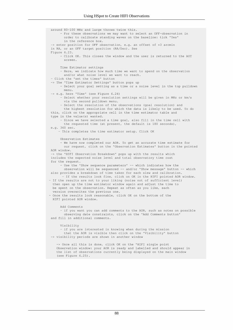
Using HSpot to Create HIFI Observations
88
around 80-100 MHz and large throws twice this. - For these observations we may want to select an OFF-observation in order to calibrate standing waves on the baseline: tick "Yes" in the reference box. -> enter position for OFF observation, e.g. an offset of +3 arcmin in RA, or an OFF target position (RA/Dec). See Figure 6.23. - Click OK. This closes the window and the user is returned to the AOT screen.
Time Estimator settings - Here, we indicate how much time we want to spend on the observation and/or what noise level we want to reach. - Click the "set the times" button -> The "Time Estimator Settings" button pops up - Select your goal setting as a time or a noise level in the top pulldown menu. -> e.g. here "Time" (see Figure 6.24) - Select whether your resolution settings will be given in MHz or km/s via the second pulldown menu. - Select the resolution of the observations (goal resolution) and the highest resolution for which the data is likely to be used. To do this, click on the appropriate cell in the time estimator table and type in the value(s) wanted. - Since we have selected a time goal, also fill in the time cell with the requested time (at present, the default is 180 seconds), e.g. 360 sec. - This completes the time estimator setup. Click OK
Observation Estimates - We have now completed our AOR. To get an accurate time estimate for our request, click on the "Observation Estimates" button in the pointed AOR window. -> the "HIFI Observation Breakdown" pops up with the results which includes the expected noise level and total observatory time cost for the request. - Use the "Show sequence parameters" -- which indicates how the observation will be sequenced -- and/or "Show message" button -- which also provides a breakdown of time taken for each slew and calibration. - If the results look fine, click on OK in the HIFI pointed AOR window. - If the results are not to your liking (noise not of sufficient level) then open up the time estimator window again and adjust the time to be spent on the observation. Repeat as often as you like, each version overwrites the previous one. - Once the results look reasonable, click OK on the bottom of the HIFI pointed AOR window.
Add Comments - if you want you can add comments to the AOR, such as notes on possible observing date constraints, click on the "Add Comments button" and fill in additional comments.
Visibility - if you are interested in knowing when during the mission that the AOR is visible then click on the "Visibility" button -> visibility periods are shown in another window
-> Once all this is done, click OK on the "HIFI single point Observation window: your AOR is ready and labelled and should appear in the list of observations currently being displayed on the main window (see Figure 6.25).
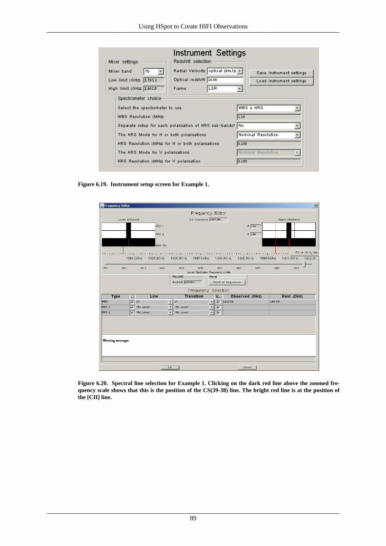
Using HSpot to Create HIFI Observations
89
Figure 6.19. Instrument setup screen for Example 1.
Figure 6.20. Spectral line selection for Example 1. Clicking on the dark red line above the zoomed fre-quency scale shows that this is the position of the CS(39-38) line. The bright red line is at the position ofthe [CII] line.
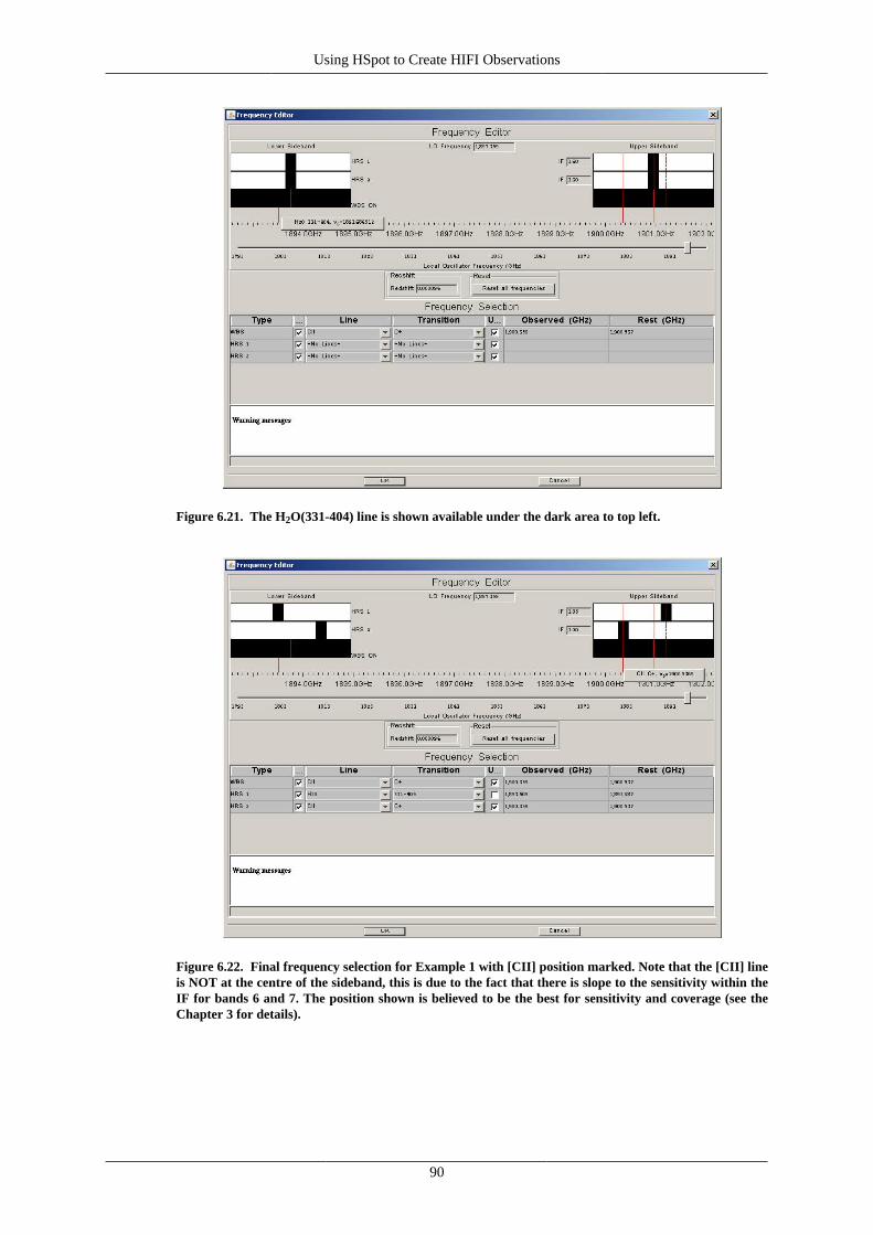
Using HSpot to Create HIFI Observations
90
Figure 6.21. The H2O(331-404) line is shown available under the dark area to top left.
Figure 6.22. Final frequency selection for Example 1 with [CII] position marked. Note that the [CII] lineis NOT at the centre of the sideband, this is due to the fact that there is slope to the sensitivity within theIF for bands 6 and 7. The position shown is believed to be the best for sensitivity and coverage (see theChapter 3 for details).
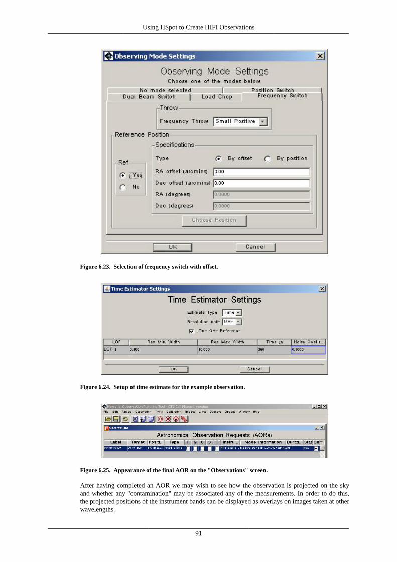
Using HSpot to Create HIFI Observations
91
Figure 6.23. Selection of frequency switch with offset.
Figure 6.24. Setup of time estimate for the example observation.
Figure 6.25. Appearance of the final AOR on the "Observations" screen.
After having completed an AOR we may wish to see how the observation is projected on the skyand whether any "contamination" may be associated any of the measurements. In order to do this,the projected positions of the instrument bands can be displayed as overlays on images taken at otherwavelengths.
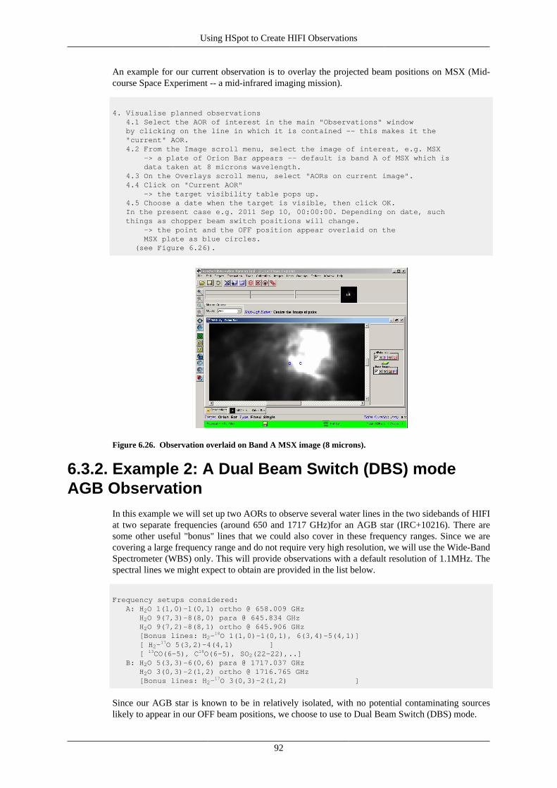
Using HSpot to Create HIFI Observations
92
An example for our current observation is to overlay the projected beam positions on MSX (Mid-course Space Experiment -- a mid-infrared imaging mission).
4. Visualise planned observations 4.1 Select the AOR of interest in the main "Observations" window by clicking on the line in which it is contained -- this makes it the "current" AOR. 4.2 From the Image scroll menu, select the image of interest, e.g. MSX -> a plate of Orion Bar appears -- default is band A of MSX which is data taken at 8 microns wavelength. 4.3 On the Overlays scroll menu, select "AORs on current image". 4.4 Click on "Current AOR" -> the target visibility table pops up. 4.5 Choose a date when the target is visible, then click OK. In the present case e.g. 2011 Sep 10, 00:00:00. Depending on date, such things as chopper beam switch positions will change. -> the point and the OFF position appear overlaid on the MSX plate as blue circles. (see Figure 6.26).
Figure 6.26. Observation overlaid on Band A MSX image (8 microns).
6.3.2. Example 2: A Dual Beam Switch (DBS) modeAGB Observation
In this example we will set up two AORs to observe several water lines in the two sidebands of HIFIat two separate frequencies (around 650 and 1717 GHz)for an AGB star (IRC+10216). There aresome other useful "bonus" lines that we could also cover in these frequency ranges. Since we arecovering a large frequency range and do not require very high resolution, we will use the Wide-BandSpectrometer (WBS) only. This will provide observations with a default resolution of 1.1MHz. Thespectral lines we might expect to obtain are provided in the list below.
Frequency setups considered: A: H2O 1(1,0)-1(0,1) ortho @ 658.009 GHz H2O 9(7,3)-8(8,0) para @ 645.834 GHz H2O 9(7,2)-8(8,1) ortho @ 645.906 GHz [Bonus lines: H2-
18O 1(1,0)-1(0,1), 6(3,4)-5(4,1)] [ H2-
17O 5(3,2)-4(4,1) ] [ 13CO(6-5), C18O(6-5), SO2(22-22),..] B: H2O 5(3,3)-6(0,6) para @ 1717.037 GHz H2O 3(0,3)-2(1,2) ortho @ 1716.765 GHz [Bonus lines: H2-
17O 3(0,3)-2(1,2) ]
Since our AGB star is known to be in relatively isolated, with no potential contaminating sourceslikely to appear in our OFF beam positions, we choose to use to Dual Beam Switch (DBS) mode.
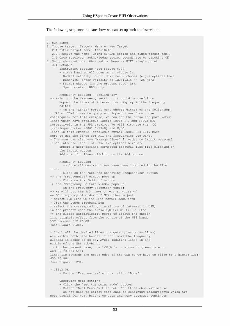
Using HSpot to Create HIFI Observations
93
The following sequence indicates how we can set up such an observation.
1. Run HSpot2. Choose target: Targets Menu -> New Target 2.1 Enter target name: IRC+10216 2.2 Resolve the name (using SIMBAD option and fixed target tab). 2.3 Once resolved, acknowledge source coordinate by clicking OK3. Setup observations: Observation Menu -> HIFI single point 3.1 Setup A Instrument setting (see Figure 6.27) - mixer band scroll down menu: choose 2a - Radial velocity scroll down menu: choose (e.g.) optical km/s - Redshift: enter velocity of IRC+10216 => -26 km/s - Frame: choose (in the present case) LSR - Spectrometer: WBS only
Frequency setting - preliminary -> Prior to the frequency setting, it could be useful to import the lines of interest for display in the frequency editor - On the "Lines" scroll menu choose either of the following: * JPL or CDMS lines to query and import lines from those catalogues. For this example, we can add the ortho and para water lines which have catalogue labels 18005 H2O and 18003 H2O respectively in the JPL catalog. We will also use the 13CO [catalogue number 29001 C-13-0] and H2
18O lines in this example [catalogue number 20003 H20-18]. Make sure to get the lines for ALL the frequencies you want. * The user can also use "Manage Lines" in order to import personal lines into the line list. The two options here are: Import a user-defined formatted spectral line file clicking on the Import button. Add specific lines clicking on the Add button.
Frequency Setting -> Once all desired lines have been imported in the line list: - Click on the "Set the observing Frequencies" button -> the "Frequencies" window pops up - Click on the "Add..." button -> the "Frequency Editor" window pops up - On the Frequency Selection table: -> we will put the H2O lines on either sides of an LO frequency of order 652 GHz, then adjust. * select H2O line in the line scroll down menu * Tick the Upper Sideband box * select the corresponding transition of interest in USB, in the present case the ortho H2O 1(1,0)-1(0,1) line -> the slider automatically moves to locate the chosen line slightly offset from the centre of the WBS band. LOF becomes 652.26 GHz (see Figure 6.28).
* Check all the desired lines (targeted plus bonus lines) are within both side-bands. If not, move the frequency sliders in order to do so. Avoid locating lines in the middle of the WBS sub-band. -> in the present case, the 13CO(6-5) -- shown in green here -- and H2-
18O(634-541) lines lie towards the upper edge of the USB so we have to slide to a higher LOF: 653.45 GHz (see Figure 6.29).
* Click OK - On the "Frequencies" window, click "Done".
Observing mode setting - Click the "set the point mode" button - Select "Dual Beam Switch" tab. For these observations we do not want to select fast chop or continuum measurements which are most useful for very bright objects and very accurate continuum
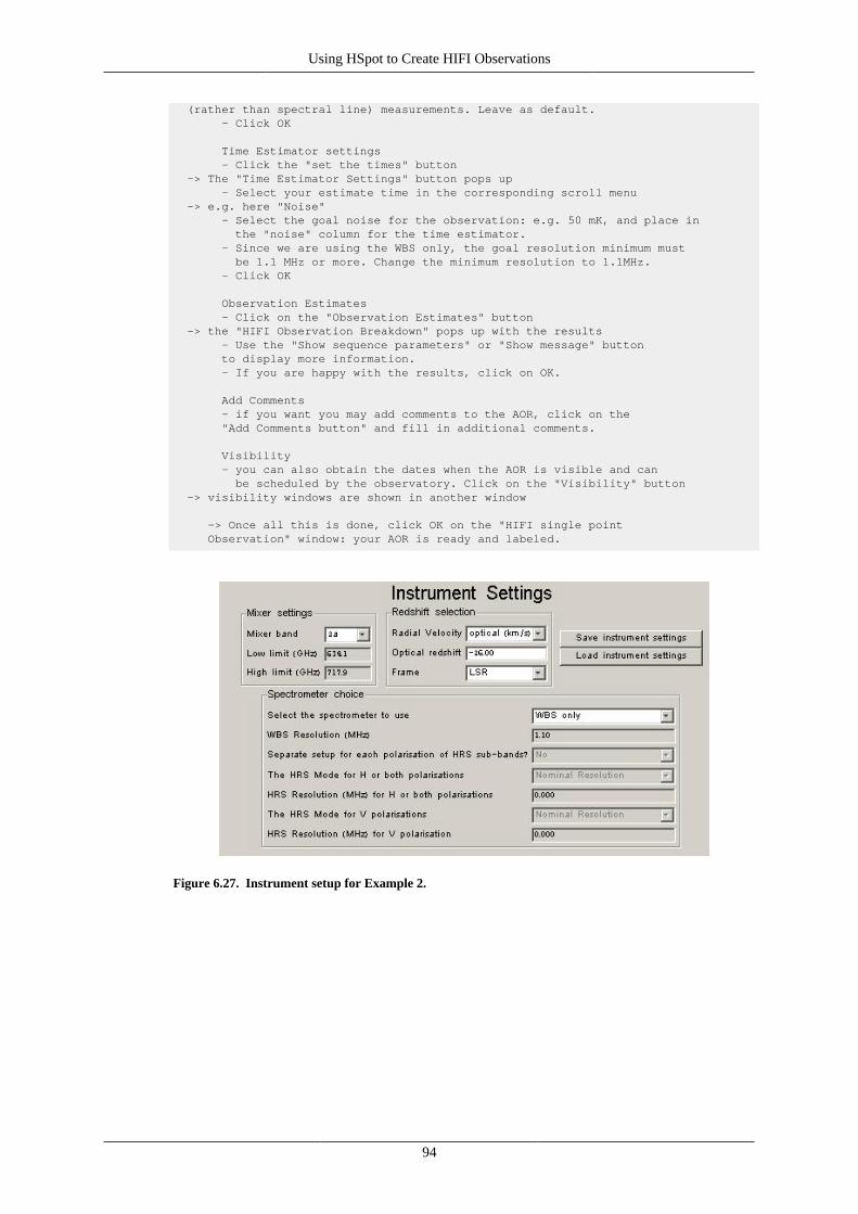
Using HSpot to Create HIFI Observations
94
(rather than spectral line) measurements. Leave as default. - Click OK
Time Estimator settings - Click the "set the times" button -> The "Time Estimator Settings" button pops up - Select your estimate time in the corresponding scroll menu -> e.g. here "Noise" - Select the goal noise for the observation: e.g. 50 mK, and place in the "noise" column for the time estimator. - Since we are using the WBS only, the goal resolution minimum must be 1.1 MHz or more. Change the minimum resolution to 1.1MHz. - Click OK
Observation Estimates - Click on the "Observation Estimates" button -> the "HIFI Observation Breakdown" pops up with the results - Use the "Show sequence parameters" or "Show message" button to display more information. - If you are happy with the results, click on OK.
Add Comments - if you want you may add comments to the AOR, click on the "Add Comments button" and fill in additional comments.
Visibility - you can also obtain the dates when the AOR is visible and can be scheduled by the observatory. Click on the "Visibility" button -> visibility windows are shown in another window
-> Once all this is done, click OK on the "HIFI single point Observation" window: your AOR is ready and labeled.
Figure 6.27. Instrument setup for Example 2.
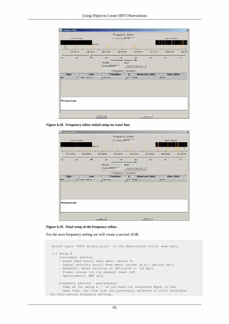
Using HSpot to Create HIFI Observations
95
Figure 6.28. Frequency editor initial setup on water line.
Figure 6.29. Final setup of the frequency editor.
For the next frequency setting we will create a second AOR.
Select again "HIFI Single point" in the Observation scroll down menu.
3.2 Setup B Instrument setting - mixer band scroll down menu: choose 7a - Radial velocity scroll down menu: choose (e.g.) optical km/s - Redshift: enter velocity of IRC+10216 => -26 km/s - Frame: choose (in the present case) LSR - Spectrometer: WBS only
Frequency setting - preliminary - Same as for setup A -- if you have not restarted HSpot in the mean time, the line list you previously selected is still available for this second frequency setting.
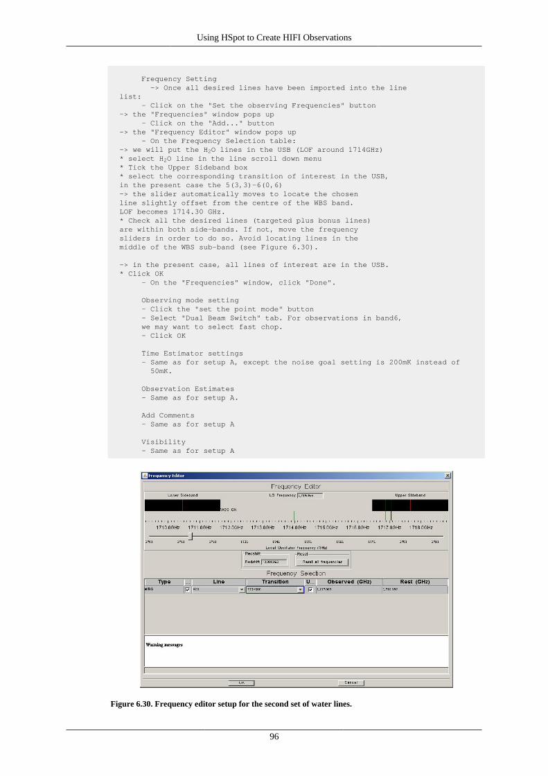
Using HSpot to Create HIFI Observations
96
Frequency Setting -> Once all desired lines have been imported into the line list: - Click on the "Set the observing Frequencies" button -> the "Frequencies" window pops up - Click on the "Add..." button -> the "Frequency Editor" window pops up - On the Frequency Selection table: -> we will put the H2O lines in the USB (LOF around 1714GHz) * select H2O line in the line scroll down menu * Tick the Upper Sideband box * select the corresponding transition of interest in the USB, in the present case the 5(3,3)-6(0,6) -> the slider automatically moves to locate the chosen line slightly offset from the centre of the WBS band. LOF becomes 1714.30 GHz. * Check all the desired lines (targeted plus bonus lines) are within both side-bands. If not, move the frequency sliders in order to do so. Avoid locating lines in the middle of the WBS sub-band (see Figure 6.30).
-> in the present case, all lines of interest are in the USB. * Click OK - On the "Frequencies" window, click "Done".
Observing mode setting - Click the "set the point mode" button - Select "Dual Beam Switch" tab. For observations in band6, we may want to select fast chop. - Click OK
Time Estimator settings - Same as for setup A, except the noise goal setting is 200mK instead of 50mK.
Observation Estimates - Same as for setup A.
Add Comments - Same as for setup A
Visibility - Same as for setup A
Figure 6.30. Frequency editor setup for the second set of water lines.
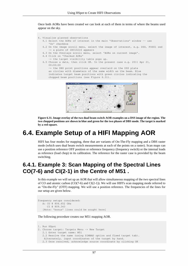
Using HSpot to Create HIFI Observations
97
Once both AORs have been created we can look at each of them in terms of where the beams usedappear on the sky.
4. Visualise planned observations 4.1 Select the AORs of interest in the main "Observations" window -- use "On" checkbox 4.2 On the Image scroll menu, select the image of interest, e.g. DSS, POSS1 red -> a plate of IRC10216 appears 4.3 On the Overlays scroll menu, select "AORs on current image". 4.4 Click on "Checked AORs" -> the target visibility table pops up. 4.5 Choose a date, then click OK. In the present case e.g. 2011 Apr 21, 00:00:00 -> the DBS point positions appear overlaid on the DSS plate as circles with diameters of the same width as the beam. Blue indicates target beam positions with green circles indicating the chopped beam positions (see Figure 6.31).
Figure 6.31. Image overlay of the two dual beam switch AOR examples on a DSS image of the region. Thetwo chopped positions are shown in blue and green for the two phases of DBS mode. The target is markedby a red square.
6.4. Example Setup of a HIFI Mapping AORHIFI has four modes for mapping, three that are variants of On-The-Fly mapping and a DBS rastermode (which uses dual beam switch measurements at each of the points on a raster). Scan maps canuse a position reference OFF position or reference frequency (frequency switch) or the internal loadsas reference (load chop) in its calibration. The reference for the raster case is provided by the beamswitching.
6.4.1. Example 3: Scan Mapping of the Spectral LinesCO(7-6) and CI(2-1) in the Centre of M51 .
In this example we will set up an AOR that will allow simultaneous mapping of the two spectral linesof CO and atomic carbon (CO(7-6) and CI(2-1)). We will use HIFI's scan mapping mode referred toas "On-the-Fly" (OTF) mapping. We will use a position reference. The frequencies of the lines forour setup are given below.
Frequency setups considered: A: CO @ 806.652 GHz CI @ 809.343 [Note: "bonus" lines could be sought here]
The following procedure creates our M51 mapping AOR.
1. Run HSpot2. Choose target: Targets Menu -> New Target 2.1 Enter target name: M51 2.2 Resolve the name (using SIMBAD option and fixed target tab). Alternately, input coordinates of the target by hand. 2.3 Once resolved, acknowledge source coordinate by clicking OK
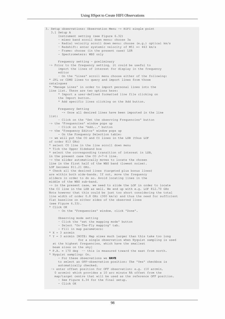
Using HSpot to Create HIFI Observations
98
3. Setup observations: Observation Menu -> HIFI single point 3.1 Setup A Instrument setting (see Figure 6.32) - mixer band scroll down menu: choose 3a - Radial velocity scroll down menu: choose (e.g.) optical km/s - Redshift: enter systemic velocity of M51 => 463 km/s - Frame: choose (in the present case) LSR - Spectrometers: WBS only
Frequency setting - preliminary -> Prior to the frequency setting, it could be useful to import the lines of interest for display in the frequency editor - On the "Lines" scroll menu choose either of the following: * JPL or CDMS lines to query and import lines from those catalogues * "Manage Lines" in order to import personal lines into the line list. There are two options here: * Import a user-defined formatted line file clicking on the Import button. * Add specific lines clicking on the Add button.
Frequency Setting -> Once all desired lines have been imported in the line list: - Click on the "Set the observing Frequencies" button -> the "Frequencies" window pops up - Click on the "Add..." button -> the "Frequency Editor" window pops up - On the Frequency Selection table: -> we will put the CO and CI lines in the LSB (thus LOF of order 813 GHz) * select CO line in the line scroll down menu * Tick the Upper Sideband box * select the corresponding transition of interest in LSB, in the present case the CO J=7-6 line. -> the slider automatically moves to locate the chosen line in the first half of the WBS band (lowest noise). LOF becomes 811.21 GHz. * Check all the desired lines (targeted plus bonus lines) are within both side-bands. If not, move the frequency sliders in order to do so. Avoid locating lines in the middle of the WBS sub-band. -> in the present case, we need to slide the LOF in order to locate the CI line in the LSB as well. We end up with e.g. LOF 812.70 GHz Note however that this could be just too short considering the total line width of order 0.8 GHz (300 km/s) and thus the need for sufficient flat baseline on either sides of the observed lines (see Figure 6.33). * Click OK - On the "Frequencies" window, click "Done".
Observing mode setting - Click the "set the mapping mode" button - Select "On-The-Fly mapping" tab. - Fill in map parameters: * X = 3 arcmin * Y = 3 arcmin [NOTE: Map sizes much larger than this take too long for a single observation when Nyquist sampling is used at the highest frequencies, which have the smallest beam sizes on the sky] * P.A. = 170 deg -- this is measured toward the east from north. * Nyquist sampling: On. - For these observations we HAVE to select an OFF-observation position: The "Yes" checkbox is automatically checked. -> enter offset position for OFF observation: e.g. (10 arcmin, 0 arcmin) which provides a 10 arc minute RA offset from the map/target centre that will be used as the reference OFF position. - See Figure 6.34 for the final setup. - Click OK
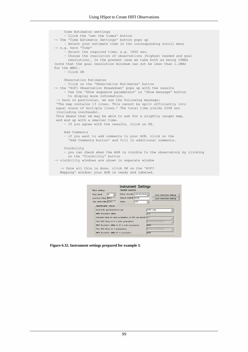
Using HSpot to Create HIFI Observations
99
Time Estimator settings - Click the "set the times" button -> The "Time Estimator Settings" button pops up - Select your estimate time in the corresponding scroll menu -> e.g. here "Time" - Select the required time: e.g. 1800 sec. - Choose the resolution of observations (highest needed and goal resolution). In the present case we take both as being 10MHz (note that the goal resolution minimum can not be less than 1.1MHz for the WBS). - Click OK
Observation Estimates - Click on the "Observation Estimates" button -> the "HIFI Observation Breakdown" pops up with the results - Use the "Show sequence parameters" or "Show message" button to display more information. -> here in particular, we see the following message: "The map contains 13 lines. This cannot be split efficiently into equal scans of multiple lines." The total time yields 2268 sec (including overheads). This means that we may be able to ask for a slightly larger map, and end up with a smaller time. - If you agree with the results, click on OK.
Add Comments - if you want to add comments to your AOR, click on the "Add Comments button" and fill in additional comments.
Visibility - you can check when the AOR is visible to the observatory by clicking on the "Visibility" button -> visibility windows are shown in separate window
-> Once all this is done, click OK on the "HIFI Mapping" window: your AOR is ready and labeled.
Figure 6.32. Instrument settings prepared for example 3.
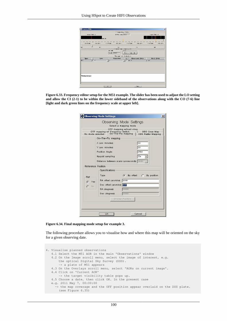
Using HSpot to Create HIFI Observations
100
Figure 6.33. Frequency editor setup for the M51 example. The slider has been used to adjust the LO settingand allow the CI (2-1) to be within the lower sideband of the observations along with the CO (7-6) line[light and dark green lines on the frequency scale at upper left].
Figure 6.34. Final mapping mode setup for example 3.
The following procedure allows you to visualise how and where this map will be oriented on the skyfor a given observing date.
4. Visualise planned observations 4.1 Select the M51 AOR in the main "Observations" window 4.2 On the Image scroll menu, select the image of interest, e.g. the optical Digital Sky Survey (DSS). -> a plate of M51 appears 4.3 On the Overlays scroll menu, select "AORs on current image". 4.4 Click on "Current AOR" -> the target visibility table pops up. 4.5 Choose a date, then click OK. In the present case e.g. 2011 May 7, 00:00:00 -> the map coverage and the OFF position appear overlaid on the DSS plate. (see Figure 6.35)
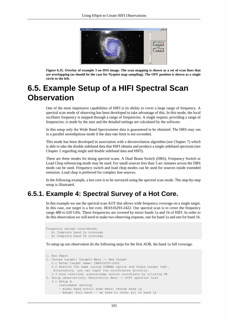
Using HSpot to Create HIFI Observations
101
Figure 6.35. Overlay of example 3 on DSS image. The scan mapping is shown as a set of scan lines thatare overlapping (as should be the case for Nyquist map sampling). The OFF position is shown as a singlecircle to the left.
6.5. Example Setup of a HIFI Spectral ScanObservation
One of the most impressive capabilities of HIFI is its ability to cover a large range of frequency. Aspectral scan mode of observing has been developed to take advantage of this. In this mode, the localoscillator frequency is stepped through a range of frequencies. A single request, providing a range offrequencies, is made by the user and the detailed settings are calculated by the software.
In this setup only the Wide Band Spectrometer data is guaranteed to be obtained. The HRS may runin a parallel serendipitous mode if the data rate limit is not exceeded.
This mode has been developed in association with a deconvolution algorithm (see Chapter 7) whichis able to take the double sideband data that HIFI obtains and produce a single sideband spectrum (seeChapter 2 regarding single and double sideband data and HIFI).
There are three modes for doing spectral scans. A Dual Beam Switch (DBS), Frequency Switch orLoad Chop referencing mode may be used. For small sources less than 3 arc minutes across the DBSmode can be used. Frequency switch and load chop modes can be used for sources inside extendedemission. Load chop is preferred for complex line sources.
In the following example, a hot core is to be surveyed using the spectral scan mode. The step-by-stepsetup is illustrated.
6.5.1. Example 4: Spectral Survey of a Hot Core.In this example we use the spectral scan AOT that allows wide frequency coverage on a single target.In this case, our target is a hot core, IRAS16293-2422. Our spectral scan is to cover the frequencyrange 488 to 620 GHz. These frequencies are covered by mixer bands 1a and 1b of HIFI. In order todo this observation we will need to make two observing requests, one for band 1a and one for band 1b.
Frequency setups considered: A: Complete band 1a coverage B: Complete band 1b coverage
To setup up our observation do the following steps for the first AOR, the band 1a full coverage.
1. Run HSpot2. Choose target: Targets Menu -> New Target 2.1 Enter target name: IRAS16293-2422 2.2 Resolve the name (using SIMBAD option and fixed target tab). Alternately, you can input the coordinates directly. 2.3 Once resolved, acknowledge source coordinate by clicking OK3. Setup observations: Observation Menu -> HIFI spectral scan 3.1 Setup A Instrument setting - mixer band scroll down menu: choose band 1a - Range: full band -- we need to cover all of band 1a
Using HSpot to Create HIFI Observations
102
- Redundancy: 6 -- this indicates how many LO frequency settings there will be within the 4GHz IF frequency range. So a setting of 6 indicates data taken every 750MHz. Higher redundancy produces higher quality results but at the cost of more observing time. - Both WBS polarizations are on -- the default (see Figure 6.36)
Mode setting - We will use the Dual Beam Switch reference mode. - No fast chop, no continuum to be used. Time Estimator settings - Select estimate to be done with a time goal in the corresponding scroll menu -> e.g. here "Time" - Input the required time in the table below: e.g. 3000 sec. For a spectral scan, a single scan can take a lot of observing time. If the input user time is less than than the minimum time possible for the request, then the returned value observation time estimate is the minimum for the input spectral scan settings.
Observation Estimates - Click on the "Observation Estimates" button -> the "HIFI Observation Breakdown" pops up with the results -> we end up here with approximately 7607 seconds for a time estimate, and a noise of 10 mK. - Use the "Show sequence parameters" or "Show message" button to display more information. - If these results are alright then click on OK. If not, then change the instrument settings and/or the time estimator settings appropriately.
Add Comments - the user may add comments to the AOR (e.g., "This AOR forms part of a survey of a hot core from 488 to 620 GHz"). To do this, click on the "Add Comments button" and fill in additional comments text.
Visibility - if you are interested in knowing when the AOR created is visible to the observatory, click on the "Visibility" button -> visibility windows are shown in another window
-> Once all this is done, click OK on the "HIFI single point Observation" window: your AOR is ready and labeled and should appear in the "Observations" window of HSpot.
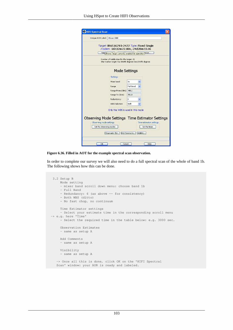
Using HSpot to Create HIFI Observations
103
Figure 6.36. Filled in AOT for the example spectral scan observation.
In order to complete our survey we will also need to do a full spectral scan of the whole of band 1b.The following shows how this can be done.
3.2 Setup B Mode setting - mixer band scroll down menu: choose band 1b - Full Band - Redundancy: 6 (as above -- for consistency) - Both WBS (ditto) - No fast chop, no continuum
Time Estimator settings - Select your estimate time in the corresponding scroll menu -> e.g. here "Time" - Select the required time in the table below: e.g. 3000 sec.
Observation Estimates - same as setup A
Add Comments - same as setup A
Visibility - same as setup A
-> Once all this is done, click OK on the "HIFI Spectral Scan" window: your AOR is ready and labeled.
104
Chapter 7. Pipeline and DataProducts Description7.1. Data to be Passed on to the User
All Herschel instrument data processing pipelines are designed to provide processing up to the point ofinstrument artifact removal (level-1). Immediately available as products from the Herschel pipelinesfor users are level-0 (raw) and level-1 data (processed). All data production and handling is donewithin the Herschel Common Science System (HCSS) environment before placing the full pipelineresults into the Herschel Science Archive (HSA). Further processing of data is possible via the DataProcessing component of the HCSS or via export to other software systems by the user.
We provide here a minimal description of pipelines and data products. Significant documentation onthe pipelines, running pipelines interactively and analysing HIFI data using the HCSS are providedwhen users download the HIPE software system. Substantial documentation is provided within thedownload.
Users are recommended to use the web interface to obtain public data from the HSA to learn aboutthe structure and format of the data provided.
Level-0 data: Raw telemetry data as measured by the instrument, minimally manipulated and put intothe mission data base/archive, often sorted and corrected for small errors. Typically, readings are inbinary units versus detector pixel number.
Level-1 data: Detector readouts calibrated and converted to physical units, as much as possible in-strument and observatory independent. In principle level-1 data processing can be done without hu-man intervention. For HIFI these are individual spectral scans with detector readings as fluxes versuswavelength. Telescope pointings are given in RA and DEC; the conversion from satellite pointingdata to RA and DEC is provided by ESA.
It should be noted that the user can run all the HIFI data pipelines interactively or in batch mode fromhis/her own local computer system using the HCSS. This means that data reprocessing can be doneby the astronomer rather than needing to be requested from the Herschel Science Centre.
7.2. Additional Observatory Meta DataAside from the raw telemetry any HIFI data product will contain appropriate meta data describingthe raw data and adding information not contained in the data themselves. The data descriptive metadata will describe e.g. the number of pixels in a spectrum, units along axes etc. Additional informationwill be items like instrument set up used, integration time, observed source, processing steps appliedto the data.
Any set of HIFI data in the database is linked to other information on the observed object, the observer,the program etc. This information is not stored in the HIFI data proper, but can be found by navigatingthe Observation Context which the standard repository for a complete set of data associaated with anobservation. When exporting HIFI data to e.g. FITS, some relevant information from these associa-tions is also copied into the FITS file.
7.3. Example HIFI data products
7.3.1. Level 0 productsThe HIFI level 0 data frame products contain simple readout counts versus channel (pixel) number.Examples of such products are shown in Figure 7.1 for typical HIFI calibration scans for the zero
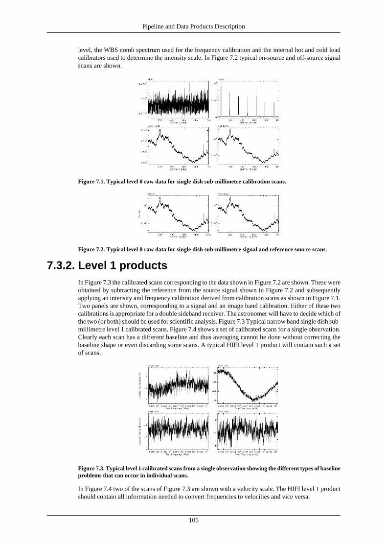
Pipeline and Data Products Description
105
level, the WBS comb spectrum used for the frequency calibration and the internal hot and cold loadcalibrators used to determine the intensity scale. In Figure 7.2 typical on-source and off-source signalscans are shown.
Figure 7.1. Typical level 0 raw data for single dish sub-millimetre calibration scans.
Figure 7.2. Typical level 0 raw data for single dish sub-millimetre signal and reference source scans.
7.3.2. Level 1 productsIn Figure 7.3 the calibrated scans corresponding to the data shown in Figure 7.2 are shown. These wereobtained by subtracting the reference from the source signal shown in Figure 7.2 and subsequentlyapplying an intensity and frequency calibration derived from calibration scans as shown in Figure 7.1.Two panels are shown, corresponding to a signal and an image band calibration. Either of these twocalibrations is appropriate for a double sideband receiver. The astronomer will have to decide which ofthe two (or both) should be used for scientific analysis. Figure 7.3 Typical narrow band single dish sub-millimetre level 1 calibrated scans. Figure 7.4 shows a set of calibrated scans for a single observation.Clearly each scan has a different baseline and thus averaging cannot be done without correcting thebaseline shape or even discarding some scans. A typical HIFI level 1 product will contain such a setof scans.
Figure 7.3. Typical level 1 calibrated scans from a single observation showing the different types of baselineproblems that can occur in individual scans.
In Figure 7.4 two of the scans of Figure 7.3 are shown with a velocity scale. The HIFI level 1 productshould contain all information needed to convert frequencies to velocities and vice versa.
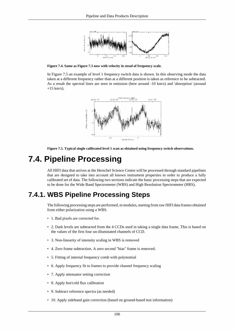
Pipeline and Data Products Description
106
Figure 7.4. Same as Figure 7.3 now with velocity in stead of frequency scale.
In Figure 7.5 an example of level 1 frequency switch data is shown. In this observing mode the datataken at a different frequency rather than at a different position is taken as reference to be subtracted.As a result the spectral lines are seen in emission (here around -10 km/s) and 'absorption' (around+15 km/s).
Figure 7.5. Typical single calibrated level 1 scan as obtained using frequency switch observations.
7.4. Pipeline ProcessingAll HIFI data that arrives at the Herschel Science Centre will be processed through standard pipelinesthat are designed to take into account all known instrument properties in order to produce a fullycalibrated set of data. The following two sections indicate the basic processing steps that are expectedto be done for the Wide Band Spectrometer (WBS) and High Resolution Spectrometer (HRS).
7.4.1. WBS Pipeline Processing StepsThe following processing steps are performed, in modules, starting from raw HIFI data frames obtainedfrom either polarization using a WBS.
• 1. Bad pixels are corrected for.
• 2. Dark levels are subtracted from the 4 CCDs used in taking a single data frame, This is based onthe values of the first four un-illuminated channels of CCD.
• 3. Non-linearity of intensity scaling in WBS is removed
• 4. Zero frame subtraction. A zero second "bias" frame is removed.
• 5. Fitting of internal frequency comb with polynomial
• 6. Apply frequency fit to frames to provide channel frequency scaling
• 7. Apply attenuator setting correction
• 8. Apply hot/cold flux calibration
• 9. Subtract reference spectra (as needed)
• 10. Apply sideband gain correction (based on ground-based test information)
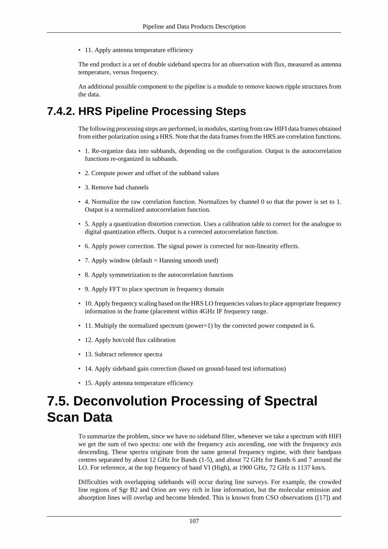
Pipeline and Data Products Description
107
• 11. Apply antenna temperature efficiency
The end product is a set of double sideband spectra for an observation with flux, measured as antennatemperature, versus frequency.
An additional possible component to the pipeline is a module to remove known ripple structures fromthe data.
7.4.2. HRS Pipeline Processing StepsThe following processing steps are performed, in modules, starting from raw HIFI data frames obtainedfrom either polarization using a HRS. Note that the data frames from the HRS are correlation functions.
• 1. Re-organize data into subbands, depending on the configuration. Output is the autocorrelationfunctions re-organized in subbands.
• 2. Compute power and offset of the subband values
• 3. Remove bad channels
• 4. Normalize the raw correlation function. Normalizes by channel 0 so that the power is set to 1.Output is a normalized autocorrelation function.
• 5. Apply a quantization distortion correction. Uses a calibration table to correct for the analogue todigital quantization effects. Output is a corrected autocorrelation function.
• 6. Apply power correction. The signal power is corrected for non-linearity effects.
• 7. Apply window (default = Hanning smooth used)
• 8. Apply symmetrization to the autocorrelation functions
• 9. Apply FFT to place spectrum in frequency domain
• 10. Apply frequency scaling based on the HRS LO frequencies values to place appropriate frequencyinformation in the frame (placement within 4GHz IF frequency range.
• 11. Multiply the normalized spectrum (power=1) by the corrected power computed in 6.
• 12. Apply hot/cold flux calibration
• 13. Subtract reference spectra
• 14. Apply sideband gain correction (based on ground-based test information)
• 15. Apply antenna temperature efficiency
7.5. Deconvolution Processing of SpectralScan Data
To summarize the problem, since we have no sideband filter, whenever we take a spectrum with HIFIwe get the sum of two spectra: one with the frequency axis ascending, one with the frequency axisdescending. These spectra originate from the same general frequency regime, with their bandpasscentres separated by about 12 GHz for Bands (1-5), and about 72 GHz for Bands 6 and 7 around theLO. For reference, at the top frequency of band VI (High), at 1900 GHz, 72 GHz is 1137 km/s.
Difficulties with overlapping sidebands will occur during line surveys. For example, the crowdedline regions of Sgr B2 and Orion are very rich in line information, but the molecular emission andabsorption lines will overlap and become blended. This is known from CSO observations ([17]) and
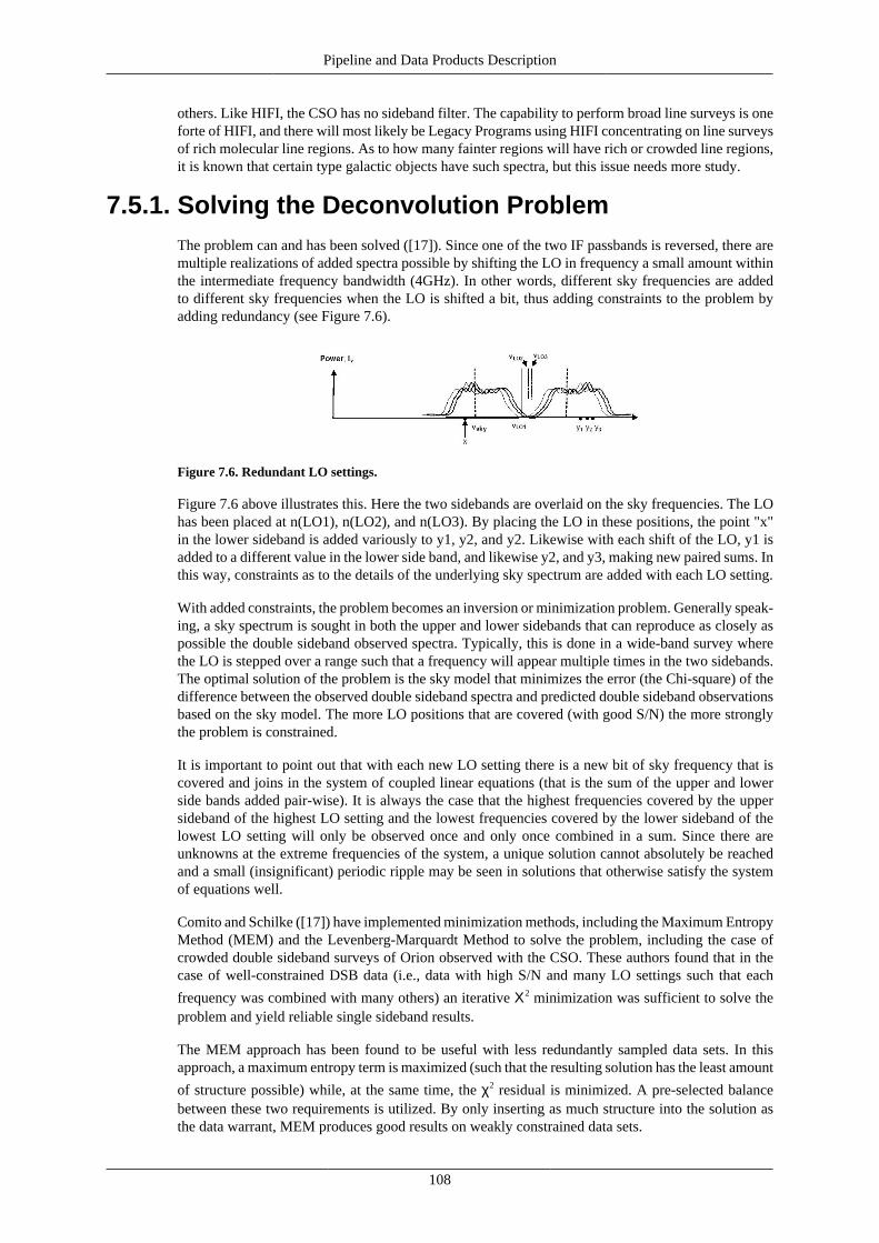
Pipeline and Data Products Description
108
others. Like HIFI, the CSO has no sideband filter. The capability to perform broad line surveys is oneforte of HIFI, and there will most likely be Legacy Programs using HIFI concentrating on line surveysof rich molecular line regions. As to how many fainter regions will have rich or crowded line regions,it is known that certain type galactic objects have such spectra, but this issue needs more study.
7.5.1. Solving the Deconvolution ProblemThe problem can and has been solved ([17]). Since one of the two IF passbands is reversed, there aremultiple realizations of added spectra possible by shifting the LO in frequency a small amount withinthe intermediate frequency bandwidth (4GHz). In other words, different sky frequencies are addedto different sky frequencies when the LO is shifted a bit, thus adding constraints to the problem byadding redundancy (see Figure 7.6).
Figure 7.6. Redundant LO settings.
Figure 7.6 above illustrates this. Here the two sidebands are overlaid on the sky frequencies. The LOhas been placed at n(LO1), n(LO2), and n(LO3). By placing the LO in these positions, the point "x"in the lower sideband is added variously to y1, y2, and y2. Likewise with each shift of the LO, y1 isadded to a different value in the lower side band, and likewise y2, and y3, making new paired sums. Inthis way, constraints as to the details of the underlying sky spectrum are added with each LO setting.
With added constraints, the problem becomes an inversion or minimization problem. Generally speak-ing, a sky spectrum is sought in both the upper and lower sidebands that can reproduce as closely aspossible the double sideband observed spectra. Typically, this is done in a wide-band survey wherethe LO is stepped over a range such that a frequency will appear multiple times in the two sidebands.The optimal solution of the problem is the sky model that minimizes the error (the Chi-square) of thedifference between the observed double sideband spectra and predicted double sideband observationsbased on the sky model. The more LO positions that are covered (with good S/N) the more stronglythe problem is constrained.
It is important to point out that with each new LO setting there is a new bit of sky frequency that iscovered and joins in the system of coupled linear equations (that is the sum of the upper and lowerside bands added pair-wise). It is always the case that the highest frequencies covered by the uppersideband of the highest LO setting and the lowest frequencies covered by the lower sideband of thelowest LO setting will only be observed once and only once combined in a sum. Since there areunknowns at the extreme frequencies of the system, a unique solution cannot absolutely be reachedand a small (insignificant) periodic ripple may be seen in solutions that otherwise satisfy the systemof equations well.
Comito and Schilke ([17]) have implemented minimization methods, including the Maximum EntropyMethod (MEM) and the Levenberg-Marquardt Method to solve the problem, including the case ofcrowded double sideband surveys of Orion observed with the CSO. These authors found that in thecase of well-constrained DSB data (i.e., data with high S/N and many LO settings such that each
frequency was combined with many others) an iterative Χ2 minimization was sufficient to solve theproblem and yield reliable single sideband results.
The MEM approach has been found to be useful with less redundantly sampled data sets. In thisapproach, a maximum entropy term is maximized (such that the resulting solution has the least amount
of structure possible) while, at the same time, the χ2 residual is minimized. A pre-selected balancebetween these two requirements is utilized. By only inserting as much structure into the solution asthe data warrant, MEM produces good results on weakly constrained data sets.
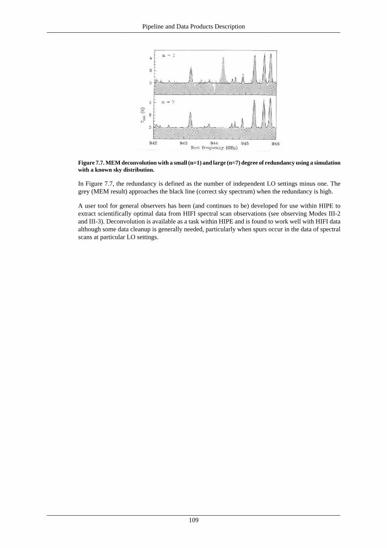
Pipeline and Data Products Description
109
Figure 7.7. MEM deconvolution with a small (n=1) and large (n=7) degree of redundancy using a simulationwith a known sky distribution.
In Figure 7.7, the redundancy is defined as the number of independent LO settings minus one. Thegrey (MEM result) approaches the black line (correct sky spectrum) when the redundancy is high.
A user tool for general observers has been (and continues to be) developed for use within HIPE toextract scientifically optimal data from HIFI spectral scan observations (see observing Modes III-2and III-3). Deconvolution is available as a task within HIPE and is found to work well with HIFI dataalthough some data cleanup is generally needed, particularly when spurs occur in the data of spectralscans at particular LO settings.
110
Chapter 8. References:[1] Jackson, B. D., Wildeman, K. J., and Whyborn, N. D. on behalf of the HIFI Focal Plane Consor-tium, "The HIFI Focal Plane Unit", 2002, Proc. 13th International Symposium on Space TerahertzTechnology, pp. 339-348, 26-28 March 2002, Harvard University, Cambridge, Massachusetts, USA.
[2] Jackson, B. D., de Lange, G., Zijlstra, T., Kroug, M., Kooi, J. W., Stern, J. A. and Klapwijk, T.M., "Low-noise 0.8-0.96- and 0.96-1.12-THz superconductor-insulator-superconductor mixers for theHerschel Space Observatory," 2006, IEEE Trans. on Microwave Theory and Techniques, vol 54, no.2, pp. 547-558
[3] Jackson, B. D., de Lange, G., Zijlstra, T., Kroug, M., Kooi, J. W., Stern, J. A. and Klapwijk, T.M., "Niobium titanium nitride-based superconductor-insulator-superconductor mixers for low-noiseterahertz receivers", 2005, Journal of Applied Physics, vol 97, no. 11, pp. 113904-113912.
[4] Delorme, Y., Salez, M., Lecomt, B., Peron, I., Dauplay, F., Feret, A., Spatazza, J., Krieg, J.-M., andSchuster, K., "Spacequalified SIS mixers for Herschel Space Observatory - HIFI band-1 instrument",2005, 16th Int.Symp.on Space THz Technology, Goteborg, Sweden (May 2-4 2005).
[5] Salez M., Delorme Y., Peron I., Lecomte B., Dauplay F., "A 30% bandwidth tunerless SIS mixerof quantum-limited sensitivity for Herschel/HIFI band 1", 2002, SPIE Proc.Vol.4855, 2002 02
[6] Cherednichenko, S., Kroug, M., Khosropanah, P., Adam, A., Merkel, H., Kollberg, E., Loudkov,D., Voronov, B., Gol'tsman, G., Huebers, H.-W., and Richter, H., "1.6 THz HEB mixer for far infraredspace telescope (Herschel)", 2002, Physica C, vol.372, pp.427-431.
[7] Cherednichenko, S., Drakinskiy, V., and Berg, T., "THz HEB heterodyne receivers for space andground based radio astronomy", 2005, Proc. Europ. Microwave Assoc., vol.1, no.3.
[8] Schieder, R., Siebertz, O., Gal, C., Olbrich, M., Schloeder, F., Bieber, R., Schmuelling, F., Tolls,V., and Horn, J., "Toward Very Large Bandwidth with Acousto-Optical Spectrometers", 2002, SPIE4855, 313-324.
[9] Belgacem, M., Ravera, L., Caux, E., Cais, P., and Cros, A., "The high resolution versatile digitalspectrometer of HIFI HSO", 2003, New Astronomy 9, 43.
[10] Ossenkopf, V., The intensity calibration framework for HIFI, 2003, ALMA Memo 442
[11] Kramer, C., "Spatial Response - Contribution to the framework document of the HIFI/Herschelcalibration group", HIFI/ICC/2003-30, version 1.8 (May 2006).
[12] HIFI ICC, "Frequency Calibration framework document," L3AB/HIFI/CAL/2003-02
[13] HIFI ICC, "HIFI Calibration Plan," LRM-ENS/HIFI/PL/2000-001
[14] Penzias A. A., Burrus C. A., 1973, ARA&A 11, 51.
[15] Schlegel D. J., et al., 1998, ApJ 500, 525
[16] Kutner M. L., Ulich B. L., 1981, ApJ 250, 341
[17] Comito, C., Schilke, P. S., 2002, A&A, 395, 357
[18] Ossenkopf, V., 2008, A&A, 495, 677
[19] Teyssier, D., Whyborn, N. D., Luinge, W. et al, 2008, in: Proceedings of the Nineteenth Interna-tional Symposium on Space Terahertz Technology, held in Groningen, Ed. Wolfgang Wild, p.132.
[20] Higgins, R., 2011, Ph.D. Thesis, NUI Maynooth.
[21] Roelfsema, P. R., et al, 2011, In-orbit Performance of Herschel-HIFI, to appear in A&A.
111
Appendix A. Change LogVersion 2.4 -- 1 June, 2011 (OT2 -- call opening)
• Chapter 5 -- Updated calibration information following lessons learned in flight. Mostly changesassociated with newly obtained sideband ratios and updated error budget.
Version 2.3 -- 31 March, 2011 (GT2 -- call opening update)
• Chapter 5 -- Updated information on spurs and representation in HSpot v5.3.
• Chapter 6 -- Complete update of screenshots and examples using HSpot v5.3.
Version 2.2 -- 20 January, 2011 (GT2 -- call opening)
• Chapter 3 -- Tsys plot updates for bands 4 (correction) and 5.
• Chapter 5 -- spur list updated in section 5.4.6.4.
• Chapter 5 -- additional spectral purity information in section 5.4.6 from original release note.
Version 2.1 -- 15 December, 2010 (AO1 -- start of observations)
• Beam profile updates in Table 5.4
• Beam efficiency measurements based on in-flight experience in Table 5.5
• Chapter 5 -- description of application of efficiencies in HIFI standard pipelines
• Chapter 5 -- updated section on spurs in band 1a, now removed in current HIFI operations
• Chapter 5 -- error budget table(s) updated.
Version 2.0 -- 20 May, 2010 (AO1)
• Substantial changes, mostly based on in-flight experience.
• Chapter 1 -- included some latest results
• Chapters 3 to 5 -- completely updated based on changes to observing modes and calibration infor-mation obtained in-flight.
• Chapter 6 -- changed figures to match changes in HSpot front end. Examples remained substantiallyunaltered.
Version 1.1 -- 14 May, 2007
• Updated sensitivity figure 3.3 in section 3.4.1
Updated section 4.2.2.3 (on cross map) to include the mode changes recently incorporated -- avail-ability of selectable cross step size.
Changed figure 6.2 to new HSpot front end
Updated section 6.2.1.1 to indicate new save and load facilities from instrument and frequencysettings for HIFI
Change Log
112
Updated section 6.2.2.3 to include information on storage of time estimates in AOR files
Changed figures 6.19, 6.27 and 6.32 to show updated front end for HIFI HSpot instrument settings.