Delft University of Technology

Semi-analytical approaches for the prediction of the noise produced by ducted windturbines

Küçükosman, Cansev

DOI10.4233/uuid:b749675c-edb1-4355-ba09-bf46278077d0Publication date2019Document VersionFinal published versionCitation (APA)Küçükosman, C. (2019). Semi-analytical approaches for the prediction of the noise produced by ductedwind turbines. https://doi.org/10.4233/uuid:b749675c-edb1-4355-ba09-bf46278077d0

Important noteTo cite this publication, please use the final published version (if applicable).Please check the document version above.

CopyrightOther than for strictly personal use, it is not permitted to download, forward or distribute the text or part of it, without the consentof the author(s) and/or copyright holder(s), unless the work is under an open content license such as Creative Commons.

Takedown policyPlease contact us and provide details if you believe this document breaches copyrights.We will remove access to the work immediately and investigate your claim.

This work is downloaded from Delft University of Technology.For technical reasons the number of authors shown on this cover page is limited to a maximum of 10.

Propositions

accompanying the dissertation

SEMI-ANALYTICAL APPROACHES FOR THE PREDICTION OF THE NOISE

PRODUCED BY DUCTED WIND TURBINES

by

Yakut Cansev KUcUKOsMAN

1. The acceleration of the flow above the fairing decreases the turbulent intensity,however, in the vicinity of the probe, this advantage is not observed (Chapter 6).

2. Analytical solutions provide insight and a good basis to improve the numericalmodels, but do not always yield a good match with experimental data (Chapter 6).

3. It is hard to obtain a mesh insensitive solution for local variables (Parr I).

4. In terms of accuracy vs computational cost balance, it is reasonable to simplifya 3D problem to a 2D one as long as the three-dimensional effects can be represented through the boundary conditions of the two-dimensional simulations(Chapter 5).

5. Listening to someone does not mean that one understands the situation unlesss/he establishes empathy.

6. Mindfulness is the key to make everyone’s life easier.

7. If we don’t take actions, we are responsible for what is coming next.

8. The essence of being an experimentalist is to acknowledge the fact that an experiment is a losing streak.

9. Life is full of ups and downs if we define it that way but in reality, it is full of opportunities.

10. Learning one’s language does not always give the opportunity to understand thehumour.

These propositions are regarded as opposable and defendable, and have been approvedas such by the promotor prof. dr. D. Casalino.

SEMI-ANALYTICAL APPROACHES FOR THEPREDICTION OF THE NOISE PRODUCED BY DUCTED

WIND TURBINES

SEMI-ANALYTICAL APPROACHES FOR THEPREDICTION OF THE NOISE PRODUCED BY DUCTED

WIND TURBINES

Dissertation

for the purpose of obtaining the degree of doctorat Deift University of Technology

by the authority of the Rector Magnificus prof,dr.ir. T.H.J,J. van der Hagenchair of the Board for Doctorates

to be defended publicly onThursday 21 March 2019 at 10:00 o’clock

by

Yakut Cansev KUçUKOSMAN

Master of Science in Turbulence,École Centrale de Lille, École Nationale Supérieure de Mécanique et d’Aerotechnique,

École Nationale Supérieure d’ingenieurs de Poitiers, Franceborn in Ankara, Turkey

This dissertation has been approved by the promotors.

Composition of the doctoral committee:

Keywords:

chairpersonDeift University of Technology, promotorvon Karman Institute for Fluid Dynamics, Belgium,copromotor

Université de Sherbrooke, CanadaÉcole Centrale de Lyon, FranceDeift University of TechnologySiemens Gamesa Renewable Energy, DenmarkDelft University of Technology, reserve member

von Karman Institute for Fluid Dynamics, Belgium

von KARMAN INSTITUTEFLUID DYNAMICS

MARIE CLJIE

wind turbine noise, semi-analytical models, ducted wind turbines

Printed by: IPSKAMP printing

Cover by: Argun çencen

Copyright © 2019 byY. C. Küçftkosman [ MIX 1Paperfrom I

FSCr.Ipol,sIb. ourceI IFSCC128610J

Rector MagnificusProf. dr. D. CasalinoProf.dr.ir. C. Schram

Independent members:Prof. dr. S. MoreauProf.dr. M. RogerProf.dr. S.J. WatsonDr. ir. S. OerlemansProf.dr. F Scarano

Other members:Dr. I. Christophe

4I I r”cIff Universityof• I L Technology

ISBN 978-94-028-1421-7

CONTENTS

1 Introduction 51.1 Background 51.2 Motivations and objectives 61.3 Thesis outline 7

2 Review of the diffuser-augmented wind turbine and noise mechanism 92.1 Working principle of diffuser-augmented wind turbines 92.2 Review of diffuser-augmented wind turbines 112.3 Wind turbine noise 14

2.3.1 Aerodynamic noise generation in general 152.3.2 Wind turbine aerodynamic noise 152.3.3 Numerical noise prediction approaches 19

I Numerical modelling 23

3 Methodology 253.1 Arniet’s analytical model for trailing edge noise 253.2 The Doppler effect 263.3 Coordinate transformation 273.4 Wall pressure spectrum models 28

3.4.1 Semi-empirical models 293.4.2 The integral model 34

3.5 CouplingwithCFD 353.5.1 RANS approaches for wind turbines 363.5.2 3D and 2D BANS approach for far-field noise of a wind turbine . 37

4 Accuracy and mesh sensitivity of RANS-based trailing-edge noise predictionusing Amiet’s theory for an isolated airfoil 414.1 Numerical simulations 42

4.1.1 Airfoil configurations 424.1.2 Computational setup 43

4.2 Mesh sensitivity 434.2.1 Pressure distribution and boundary layer profiles 434.2.2 Calculation of the global variables 454.2.3 Prediction of the wall-pressure spectra and far-field trailing edge

noise 494.3 Effect of the probe location along the airfoil 564.4 Conclusions 60

V

vi CONTENTS

5 Application to DAWT

5.1 3D Numerical simulation

5.1.1 Computational setup 64

5.1.2 Mesh Sensitivity

5.2 2D isoradial approach

5.2.1 Computational setup

5.2.2 Convergence due to the number of strips

5.2.3 Improving the inflow conditions

5.3 Comparison of the 3D and 2D computations

5.3.1 Inlet velocity profiles

5.3.2 Pressure distribution and boundary layer profiles

5.3.3 Prediction of the wall-pressure spectra and far-field trailing edgenoise 80

5.4 Conclusions 84

II Experimental work 89

6 A remote microphone technique for aeroacoustic measurements in largewind tunnels 91

6.1 Introduction 92

6.2 Microphone fairing 93

6.3 Line-cavity response model

6.3.1 Design of the fairings

6.3.2 Calibration Procedure

6.4 Aerodynamic effects of the fairing on the acoustic measurements

6.4.1 Aerodynamics6.4.2 Acoustic measurements

6.4.3 Application: Contra-rotating rotor measurements

6.5 Conclusions and perspectives

7 An investigation on the effect of the inflow quality

7.1 Introduction

7.2 Experimental setup, acquisition chain, and post-processing

7.2.4 Acquisition chain and post-processing 119

7.3 Power measurements 119

7.4 Acoustic measurements 120

7.5 Conclusions 123

8.1 Summaryandrnainresults

8.2 Future research and possible further improvements

63

64

64

67

67

69

70

74

75

76

94

95

97

98

99

100

107

108

7.2.1 Building and wind turbine models

7.2.2 Wind turbine characterization

7.2.3 Atmospheric boundary layer type

111

111

113

113

115

116

8 Conclusion 129

129

131

A Global boundary layer variables with respect to probe location

B Boundary layer proffles from 3D simulationB.1 Mesh sensitivityB.2 Boundary layer comparison between 2D and 3D simulations.B.3 Global boundary layer variables

C Building Integrated Wind TurbineC.1 Building integrated wind turbine model

C.1.1 Building moduleC.1.2 Duct moduleC.1.3 Wind turbine module

C.2 Power measurementsC.3 Acoustic measurementsReferences

Curriculum Vita 163

CONTENTS vii

133

135135136136

141141141141142142143146

NOMENCLATURE

Acronyms

1/2/3D One/Two/Three Dimensional

a.o.a Angle of Attack

ABL Atmospheric Boundary Layer

AMI Arbitrary Mesh Interface

APG Adverse Pressure Gradient

BATMAN Broadband And Tonal Models for Airfoil Noise

BEM Blade Element Momentum

BJWT Building Integrated Wind Turbines

BPF Blade Passing Frequency

CAD Computer-Aided Design

CFD Computational Fluid Dynamics

CPU Central Processing Unit

CROR Contra-rotating Open Rotor

DAWT Diffuser Augmented Wind Turbine

FPG Favorable Pressure Gradient

FWH Ffowcs Williams and Hawkings

HWA Hot Wire Anemometer

MRF Multiple Reference Frame

PIV Particle Image Velocimetry

PSD Power Spectrum Density

RANS Reynolds Averaged Navier-Stokes

RPM Random Particle-Mesh

RSNM HANS-based Statistical Noise Model

x NOMENCLATURE

SMM Sliding Mesh Method

SNGR Stochastic Noise Generation and Radiation

SPL Sound Pressure Level

SRF Single Reference Frame

SRS Scale-Resolving Simulation

TI. Turbulence Intensity

TKE Turbulent Kinetic Energy

VKI von Karman Institute for Fluid Dynamics

WPS Wall-Pressure Spectrum

ZPG Zero Pressure Gradient

Coefficients

Cf Skin friction coefficient I-I

C, Pressure coefficient L-l

Gpo wer Power coefficient 1-]

Greek Symbols

fJ Clauser’s parameter [-I

A Rotta-Caluser parameter [-I

6 Boundary layer thickness [ml

6* Displacement thickness [ml

A Zagarola-Smits’parameter I-I

e Turbulent dissipation lrn2/s3]

y Specific heat ratio I-I

K von Karman constant I-I

A Eddy size [ml

A Acoustic wavelength [m[

£ Aeroacoustic transfer function I-I

p Dynamic viscosity [Pa

v Kinematic viscosity [rn2/s[

NOMENCLATURE xi

12 Specific turbulence dissipation rate Il/s]

w Angular frequency Il/s]

flrot Angular velocity [rad/sI

cb Wall-pressure PSD dB/Hz

fl Cole’s wake parameter I-]

‘1’ Azimuthal angle Irad]

p Density 1kg/rn3]

Wall shear stress [Pa/rn2]

0 Momentum thickness Im]

e Polar observation angle Irad]

u Friction velocity Im/s]

Roman Symbols

c chord of the blade or airfoil ]mj

co Speed of sound lm/s]

d span [m]

H Shape factor 1-1

J Bessel function 1-]

k Acoustic i,ravenumber lnf 1]

k Turbulent kinetic energy 1rn2/s2]

l Spanwise corre]ation length [ml

M Mach number 1-]

Pr Prandtl number 1-]

q Dynamic pressure [Pal

R Distance between source and observer [ml

Rr Ratio of the outer to inner time scales [ml

Re Reynolds number 1-]

Far-field acoustic PSD [dB/hz]

St Sthrouhal number [-I

xii NOMENCLATURE

U Axial velocity [rn/si

U Convective velocity [rn/si

Ue External velocity [rn/sI

U free-stream velocity [rn/si

B Nurnber of blades I-i

b Corcos constant I-]

p Pressure [Pa]

X, Y, Z Observer coordinate system Irni

x, y, z Source coordinate system [ml

Subscripts

0 Local free-stream value

cc Free-stream value

r,O,z Radial, azimuthal, axial coordinates

x, y, z Streamwise, normal-to-wall and spanwise coordiantes

ABSTRACT

The integration of wind turbines into urban environments is a challenging task due tothe reduced wind speed and high turbulence levels caused by the surface resistance,as well as limited spacing. If a specific building arrangement is explored, an improvement in wind speed can be obtained. This would be especially beneficial for tall buildings where a wind turbine can be placed on the roof, side, or through a duct. However,the main problem associated with the integration of wind turbines is the acoustic annoyance. Therefore, the focus of this thesis is twofold. First, a robust, accurate, andlow computational cost numerical methodology is proposed to predict the trailing edgenoise for a ducted wind turbine. Second, a measurement device is developed to acquirenoise emitted by a rotating machine where the duct surface cannot be altered. An investigation of the incoming flow on the noise emitted by a building-integrated wind turbineis conducted by different aerodynamic roughness lengths.

The far-field trailing-edge noise prediction by the Amiet analytical theory is appliedfor two isolated airfoils, the NACAOO12 at 0° and the DU96-W180 at 4°. The comparison of the wall-pressure spectrum is performed by using the state-of-art semi-empiricalmodels; Goody, Rozenberg, Kamruzzaman, Catlett, Hu & Herr and Lee, and an integralmodel from Panton & Linebarger. A sensitivity analysis of the wall-pressure spectrumand far-field noise prediction based on different mesh resolutions is investigated andthe far-field results are validated with experimental data. Furthermore, another analysisis performed by varying the probe location to quantify the sensitivity of the wall -pressurespectrum obtained by different models as well as the corresponding far-field noise predictions.

The extended variant of Schlinker and Amiet theory is applied to a full scale commercial ducted wind turbine. The three-dimensional Reynolds Averaged Navier-Stokessimulation with a Multiple Reference Frame is performed to obtain the flow field. Thefar-field noise is predicted by a strip theory by neglecting the scattering due to the presence of the diffuser. To reduce the three-dimensional computational cost, a two dimensional isoradial approach is proposed and applied to the same configuration withoutconsidering the flow acceleration due to the diffuser and nacelle. To reproduce the flowacceleration due to the diffuser and nacelle, a two dimensional axisymmetric simulation without the presence of a blade is conducted. Several locations obtained from thissimulation are then imposed as an inlet condition for the two dimensional isoradial approach. A comparison between the three and two dimensional approaches is assessedby the wall-pressure spectrum and the far-field noise prediction obtained upstream anddownstream of the blade.

Experimental considerations regarding a noise measurement technique of a ductedwind turbine and the assessment of the noise emitted by a building-integrated wind turbine in an urban environment are investigated. The former study focuses on a development of a fairing based on a remote microphone technique. The fairing is designed as a

1

2 — ABSTRACT

streamlined proffle to avoid additional disturbances as well as to reduce the turbulencelevel. The microphone is located inside of the fairing and connected to the surroundingswith a pipe-cavity system. The system is modelled analytically and compared with thesystem response function. The investigation of the fairing is performed aerodynamicallyand aeroacoustically with different wind speeds and turbulence levels. Later, this deviceis validated through with a practical application. The latter study investigates the effectof different incoming flows both in magnitude and turbulence intensity on the noiseemission in the case of a building integrated wind turbine placed through a duct. Theacoustic measurements are performed for two different incoming flow speeds and sixdifferent wind directions with nine microphones. Furthermore, the power efficiency ofthe in-duct wind turbine is compared to another wind turbine, which is placed on thetop of a model building.

ABSTRACT

De integratie van windturbines in stedelijke omgeving is een uitdagende taak vanwegede verminderde windsnelheid, de hoge turbulentie veroorzaakt door de bebouwdeomgeving en de beperkte ruimte. Indien een specifieke bouwinrichting wordt onderzocht, kan een verhoging in windsnelheid verkregen worden. Dit zou vooral voordeligzijn voor hoge gebouwen waar een windturbine op het dak, de zijkant of in een openingkan worden geplaatst. Toch is het grootste probleem de akoestische hinder geassocieerdaan de integratie van windturbines. Bijgevolg is de focus van dit proefschrift tweeledig.Eerst wordt er een robuuste, nauwkeurige nurnerieke methodologie voorgesteld metlage rekenkundige kost om het geluid van de vleugelachterrand te voorspellen voor eenwindturbine in een opening. Ten tweede wordt een niet-intrusief meetapparaat ontwikkeld om het uitgezonden geluid afkomstig van de roterende machine op te meten.Een onderzoek van de inkomende vind stroom op het geluid uitgezonden door eengebouw-geIntegreerde windturbine wordt uitgevoerd met verschillende aerodynamische ruwheidslengtes.

De voorspelling van het verre-veld vleugelachterrand geluid door de Amietanalytische theorie wordt toegepast voor twee geIsoleerde schoepen, de NACAOO12 opOXen de DU96-W180 op 4X. De vergelijking van het wand-drukspectrum wordt uitgevoerd met behuip van state-of-art, semi-empirische modellen; Goody, Rozenberg, Kamruzzaman, Catlett, Hu & Herr en Lee, en het volledig model van Panton & Linebarger.Een gevoeligheidsanalyse van het wanddrukspectrum en verre-veld geluidsvoorspellingwordt onderzocht op basis van verschillende grid resoluties en de verre-veld-resultatenworden gevalideerd met experimentele gegevens. Verder wordt nog een analyse uitgevoerd door de locatie van de sonde te variëren om de gevoeligheid van het wanddrukspectrum, verkregen door verschillende modellen, evenals de bijbehorende verre-veld geluidvoorspellingen, te kwantiflceren.

De uitgebreide variant van de Schlinker en Amiet-theorie wordt toegepast op eencommerciële windturbine geplaatst in een opening, en dit op volledige schaal. Dedriedimensionale Reynolds Averaged Navier-Stokes simulatie met een ‘Multiple Reference Frame’ wordt uitgevoerd om het stroomveld te verkrijgen. Ret verre-veld geluidwordt voorspeld door een striptheorie door de verstrooiing vanwege de aanwezigheidvan de diffuser te verwaarlozen. Om de driedimensionale computerkosten te verminderen wordt er een tweedimensionale isoradiale benadering voorgesteld en toegepastop dezelfde configuratie zonder rekening te houden met de stroomversnelling als gevolgvan de diffuser en de nacelle. Om de stroomversnelling door de diffuser en de nacellete reproduceren, wordt een tweedimensionale asymmetrische simulatie zonder schoepuitgevoerd. Verschillende locaties verkregen uit deze simulatie worden dan opgelegdals inlaatvoorwaarde voor de tweedimensionale isoradiale benadering. Een vergelijkingtussen de drie- en tweedimensionale benaderingen wordt uitgevoerd door het wanddrukspectrum en de voorspelling van het verre-veld geluid verkregen stroomopwaarts

3

4 ABSTRACT

en stroomafwaarts van het blad te vergelijken.Experimentele overwegingen met betrekking tot een geluidsmeettechniek van een

windturbine geplaatst in een opening en de beoordeling van het geluid van een gebouwgeIntegreerde windturbine in een stedelijke omgeving worden onderzocht. De vorigestudie richt zich op de ontwikkeling van een kap gebaseerd op een microfoontechniek op afstand. De kap is ontworpen als een gestroomlijnd profiel om extra stormgen te voorkomen en om de turbulentie te verminderen. De microfoon bevindt zichin de kap en is verbonden met de omgeving dankzij een openingholtesysteem. Hetsysteem is analytisch gemodelleerd en vergeleken met de responsfunctie van het systeem. Een aerodynamisch en aeroakoustisch onderzoek van de stroomlijnkap wordtuitgevoerd met verschillende windsnelheden en turbulentieniveaus. Vervolgens wordtdit apparaat gevalideerd dankzij een praktische toepassing, Deze studie onderzoekthet effect van verschillende inkomende vind stromen, zowel in grootte als turbulentieintensiteit, op het uitgezonden geluid in bet geval van een gebouw-geIntegreerde wind-turbine geplaatst in een opening. De akoestische metingen worden uitgevoerd voor tweeverschillende inkomende stroomsnelheden en zes verschillende windrichtingen met negen microfoons. Verder wordt de stroomefficiëntie van de windturbine in de openingvergeleken met een andere windturbine, geplaatst boven op een modelgebouw.

1INTRODUCTION

This chapter is devoted to a brief introduction of the thesis followed by the objectivesand outline.

1.1. BAcKGRouNDThe energy demand due to urbanization and industrialization has raised in recentyears 11091. As stated by the United Nations in 2007 [1371, the energy consumption incities was found to be around 75% which will increase due to migration to the citiesfrom the rural areas in developing countries [11. If the traditional energy production approach remains unchanged, the depletion of fossil fuels will result in a higher cost [1461as well as green-house gas emission causing environmental problems 11061. To overcome these issues, it is necessary to find sustainable and renewable energy solutions forthe future. Since a great amount of energy consumption occurs in a city, it would beeffective and efficient to generate power within them. That will also help to reduce theuse of transmission and distribution infrastructure throughout the generation of powerto the consumer as well as the transmission losses. In recent years, a lot of care has beentaken to investigate and improve the wind energy applications in urban areas as an alternative energy resource.

The assessment of wind energy in urban environments has interesting challengescompared to open terrains. Firstly, the resistance caused by buildings in urban environments reduces the wind speed and produces a higher turbulence level with rapid fluctuations both in magnitude and direction [52, 106, 1Bl. Secondly, the limited space inthe urban environment prevents installation of large wind turbines. Even though the incoming wind speed and turbulent inflow conditions for the urban boundary layer arehighly dependent on the atmospheric conditions, the effect of urban geometry overcomes them, especially over the surface layer, which can be approximated as 10% of thetotal atmospheric boundary layer thickness [183]. Therefore, specific building arrangements can also be used to alter the wind flow within the urban canopy to further improvethe wind energy potential. As can be expected, tall buildings provide better conditions

5

6 1. INTRODUCTION

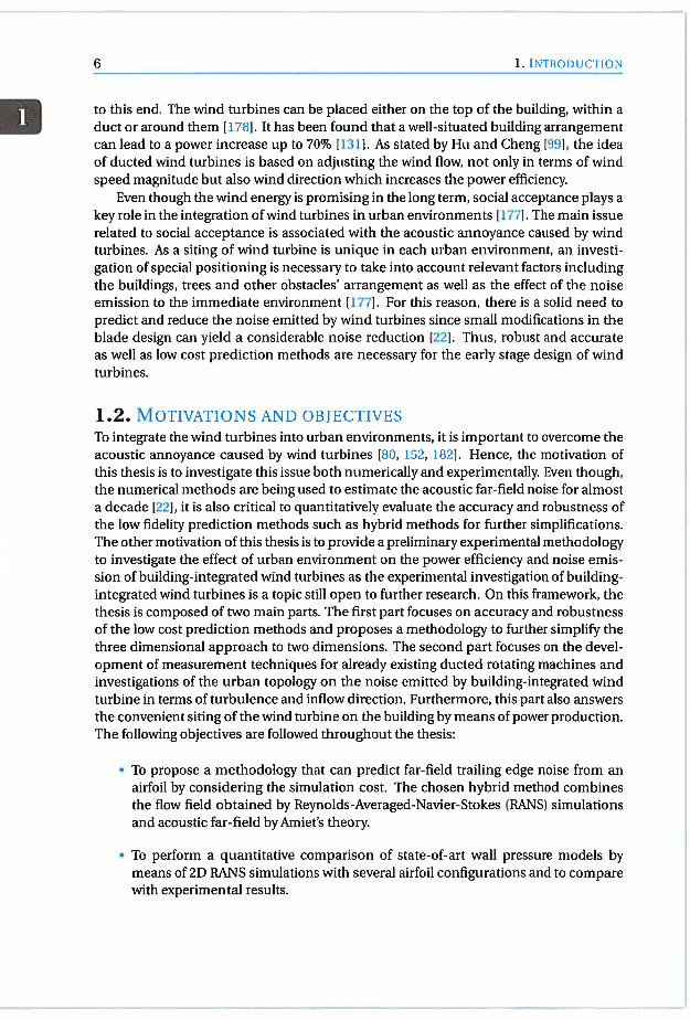
to this end. The wind turbines can be placed either on the top of the building, within aduct or around them [1781. It has been found that a well-situated building arrangementcan lead to a power increase up to 70% [1311. As stated by Ru and Cheng [991, the ideaof ducted wind turbines is based on adjusting the wind flow, not only in terms of windspeed magnitude but also wind direction which increases the power efficiency.

Even though the wind energy is promising in the long term, social acceptance plays akey role in the integration of wind turbines in urban environments [1771. The main issuerelated to social acceptance is associated with the acoustic annoyance caused by windturbines. As a siting of wind turbine is unique in each urban environment, an investigation of special positioning is necessary to take into account relevant factors includingthe buildings, trees and other obstacles’ arrangement as well as the effect of the noiseemission to the immediate environment [1771. For this reason, there is a solid need topredict and reduce the noise emitted by wind turbines since small modifications in theblade design can yield a considerable noise reduction [221. Thus, robust and accurateas well as low cost prediction methods are necessary for the early stage design of windturbines.

1.2. MOTIVATIONS AND OBJECTIVES

To integrate the wind turbines into urban environments, it is important to overcome theacoustic annoyance caused by wind turbines [80, 152, 1821. Hence, the motivation ofthis thesis is to investigate this issue both numerically and experimentally. Even though,the numerical methods are being used to estimate the acoustic far-field noise for almosta decade [22], it is also critical to quantitatively evaluate the accuracy and robustness ofthe low fidelity prediction methods such as hybrid methods for further simplifications.The other motivation of this thesis is to provide a preliminary experimental methodologyto investigate the effect of urban environment on the power efficiency and noise emission of building-integrated wind turbines as the experimental investigation of building-integrated wind turbines is a topic still open to further research. On this framework, thethesis is composed of two main parts. The first part focuses on accuracy and robustnessof the low cost prediction methods and proposes a methodology to further simplify thethree dimensional approach to two dimensions. The second part focuses on the devel-opment of measurement techniques for already existing ducted rotating machines andinvestigations of the urban topology on the noise emitted by building-integrated windturbine in terms of turbulence and inflow direction. Furthermore, this part also answersthe convenient siting of the wind turbine on the building by means of power production.The following objectives are followed throughout the thesis:

• To propose a methodology that can predict far-field trailing edge noise from anairfoil by considering the simulation cost. The chosen hybrid method combinesthe flow field obtained by Reynolds-Averaged-Navier-Stokes (RANS) simulationsand acoustic far-field byAmiet’s theory.

• To perform a quantitative comparison of state-of-art wall pressure models bymeans of 2D HANS simulations with several airfoil configurations and to comparewith experimental results.

1.3. THEsIs OUTLINE 7

To conduct a grid sensitivity analysis for RANS simulations to quantify the robustness and accuracy of the wall-pressure models as well as the far-field noise prediction.

• To extend the existed model for a full scale wind turbine and to propose a furthersimplification of the 3D method to a 2D.

• To develop a measurement device based on a remote microphone technique toacquire the noise emitted by ducted rotating machines.

• To asses the effect of the urban environment on the noise emission by a building-integrated wind turbine.

1.3. THEsIs OUTLINEThe thesis is composed of two main parts that consist of numerical and experimentalconsiderations of ducted wind turbines, defined as Part I and Part II. The introductionis followed by Chapter 2, which presents a review of a diffuser-augmented wind turbineand noise mechanism. After Chapter 2, Part I starts with the numerical methodologyfor both two and three dimensional techniques (Chapter 3). The accuracy and meshsensitivity of HANS based trailing edge predictions using Arniet’s theory is presented inChapter 4. Part I is finalized with Chapter 5, which presents numerical results for a full-scale ducted wind turbine. Part II is focused on experimental considerations of ductedwind turbines, including development of a measurement device based on a remote microphone technique (Chapter 6) and the investigation of inflow conditions on the windturbine efficiency (Chapter 7). Finally, a brief summary of the obtained main resultsalong with the conclusions and the possible future work are presented in Chapter 8.

2REVIEW OF DIFFUSER-AUGMENTED

WIND TURBINE AND NOISE

MECHANISM

In this chapter, the basic working principle of conventional and diffuser-augmentedwind turbine (DAWT) will be explained. Later, the development of ducted wind turbinesas well as the general noise mechanism observed in wind turbines without a duct will beexplained. Finally, the present numerical noise prediction methods will be discussed.

2.1. WORKING PRINCIPLE OF DIFFUSER-AUGMENTED WIND

TURBINES

The wind turbine rotor extracts energy by slowing down passing wind. To obtain a 100%efficient wind turbine, the wind speed downstream the wind turbine has to be zero.However, that would prevent the upstream wind from moving through the turbine whichcauses the turbine stop spinning. According to Betz’s law 1231, the maximum kinetic energy a bare wind turbine can extract is 16/27 0.59 which is known as the Betz limit. Theaxial velocity and pressure distributions on the centreline are shown in Fig. 2.1. It can beobserved that for the maximum operating conditions, the flow velocity upstream of therotor decreases to U, where U is the free-stream velocity, as the cross sectional areaof the stream tube increases. At the downstream side, the cross-sectional area is twicethe disk area which results in the velocity decreasing further down to U.

In order to exceed the Betz limit, the power augmentation can be performed in twoways. The first one is to use a vortex generator to create a low-pressure region to accelerate the flow as shown in Fig. 2.2. The second method is to use an annular lifting devicewhose suction side is pointed inwards to create a lift force which increases the velocityat the centerline as shown in Fig. 2.3.

9

10 2. REvIEw OF THE DIFFUSER-AUGMENTED WIND TURBINE AND NOISE MECHANISM

a)Po

C

_3/91/2VP2 Po

-oDCD

.5C

> Vw3

1— Va,

CD

<2A

Axial Distance

Figure 2.1: Ideal axial pressure, velocity and disk area variations over a bare wind turbine rotor [1841.

vortex generation by a brim —.

throat I

inlet shrotsiN —blade low-presawe region

draws more windwind.

elIe(hub)pressse recovery

byadiffliner

A

Figure 2.2: Flow around a wind turbine with a vortex Figure 2.3: Flow around a wind turbine with a difgenerator 11391. fuser 1881.

2.2. REvIEW OF DIFFUSER-AUGMENTED WIND TURBINES 11

2.2. REvIEw OF DIFFUSER-AUGMENTED WIND TURBINESIn the 1920s, the first development of ducted wind turbines was acknowledged by Betz[24]. He had formulated the correct theory with a restrictive assumption in which heassumed the exit static pressure is equal to the ambient pressure. He concluded thatducted wind turbines were uneconomical for practical applications. In the 1 950s, Sanuki[1631 published the first experimental results for ducted wind turbines and was followedby Iwasaki [107]. They both found an increase in power output compared to bare windturbines. Independently, Lilley et al. [124] demonstrated, based on the momentum andvortex theories for a ducted wind turbine, that the augmented power output was explained by an increase in axial velocity and a decrease of tip losses. In the report, theyproposed the ideal shrouded windmill by considering the cost and stated an increase of65% power output compared to the unshrouded windmill. Moreover, further increase ofthe power output could be achieved by adding an aerodynamic surface at the exit of thediffuser. Earlyinthe 1960s, anlsraeligroup [114,115] achievedapoweraugmentationbya factor of 3.5 with a longer shroud design which was inconvenient for commercial applications due to high cost of the duct length. A shorter duct with the same exit area ratiorequires a rapidly diverging diffuser. As a drawback, this would cause the flow to separate, and hence, a reduction in the performance. To overcome the separation, gurneyflaps were implemented at the duct outlet to reduce the exit pressure. Igra [102, 103, 104]realized that the power augmentation was due to sub-atmospheric pressure at the exit,thereby increasing the mass flow.

At the same time, Foreman [73, 76, 771 was focusing on Diffuser Augmented WindTurbines (DAWTs) to find alternative energy sources due to the oil crisis in 1974. In contrast to other researchers, the attempt was to control the boundary layer to create a jetflow by applying slots. The energized flow entering through the slots helps to delay orprevent flow separation, which allows shorter duct lengths and larger outlet-to-inlet arearatio DAWTs. They also observed that the separation in the diffuser was delayed havingan actual wind turbine within the duct instead of a gauze screen (sometime used to represent the rotor pressure drop) since the swirling flow at the wake of the rotor enhancedmomentum transfer to the boundary layer. Gilbert et al. [77] emphasized that the newgeneration DAWTs could provide twice the power output and be 50% cheaper than aconventional wind turbine with the same diameter and same wind speed.

By consequence of these outcomes, DAWTs became economically attractive. However, despite a strong academic interest [55, 72, 121, 127, 128, 193] the commercial exploitation of DAWTs wasn’t attempted before 1995. Vortec Energy Limited took the initiation on the development of Vortec 7 DAWT. Based on Foreman’s design [149, 1501, aprototype was built with a 17.3 meter height and optimization was performed by CFDwith a comparison of small scale experiments. The power augmentation was expectedto reach about a factor of 9, but the full-scale Vortec 7 achieved only a factor of about 2.4.One of the reasons was that the exit velocity was assumed to be uniform in the calculations. On the contrary, the full-scale model demonstrated high speed regions at the tipand lower at the hub, which reduced the power output [148].

Hansen et al. [90] compared the theoretical expression for the power coefficient as afunction of thrust coefficient with CFD computations of a bare turbine and concludedthat the actuator disk theory was applicable to model the rotor. Moreover, he confirmed

12 2. REvIEW OF THE DIFFUSER-AUGMENTED WIND TURBINE AND NOISE MECHANISM

that the Betz limit can be exceed using a diffuser. However, van Bussel [1911 emphasizedthat the calculation of the power coefficient led to an unrealistic power augmentation.He suggested that the power coefficient must be normalized using the maximum shroudarea, which reduces the power coefficient to below the Betz limit rather than the rotorarea as in a bare wind turbine calculation. Jamieson [1081 reformulated the momentumtheory to define an optimal power extraction, equal to 0.89 of the power available in therotor streamtube far downstream.

Another mechanism so-called “flanged diffuser” has been investigated both experimentally and numerically byAbe et al. [1], Abe and Ohya 121, Ohya et al. [140], and Ohyaand Karasudani 11391. In this concept, a brim was attached to the exit of diffuser, creating a large scale flow separation. As a consequence of the separation, a low-pressurezone occurs which draws more mass through diffuser compared to a diffuser without aflange. The numerical results obtained by a custom turbulence model, developed andtuned for this purpose, showed an accurate prediction of velocity and pressure profilesin comparison with experimental data [1, 21. The experimental prototype of “Wind-Lensstructure” with a length-to-diameter ratio of 1.47 produces 4-5 times more power thana conventional wind turbine 11401. A new design of a compact brimmed diffuser witha length-to-diameter ratio from 0.1 to 0.371 achieved a power output of 2.5 times largerthan a bare diffuser. Several wind turbines have been installed around China to examinethe practical application 11391 (see Fig. 2.4(a-b)) of this design.

Particle Image Velocimetry measurements were performed by Toshimitsu et al. 11891and Kardous et al. 11121 for a diffuser with a flange. Toshimitsu et al. [1891 found that theacceleration of the flow is due to the separation vortices behind the flange which led toa power increase of 2.6 times larger than a bare wind turbine. Similarly, Kardous et al.[112] compared several flange heights without the blade and concluded that the windvelocity increases by about 64% to 81% for a diffuser with a flange and 58% for a diffuserwithout a flange.

A semi-analytical method was developed by Bontempo and Manna 128] and Bontempo et al. [27] to determine an exact solution of an axisymmetric, potential flow usinga Green’s function. The difficulty of this approach is to determine the turbine loadingas a function of a stream function. To overcome this, an iterative approach is applied toobtain the flow-field.

Recently, CFD calculations were performed by Aranake et al. [12, 13] for the sameshrouded wind turbine as 127, 281, in order to compare the predictions of the existinglow-order models. Later, axisymmetric BANS simulations were performed with an actuator disc model. It is found that the Betz limit is exceed by a factor of 1.43 based on themaximum shroud area [111.

The commercial donQi Urban WindmillThas been developed extensively by theDelft University of Technology (see Fig. 2.4(c)) [184, 192]. This diffuser is an annularwing with the suction side pointing inwards which increases the velocity through theduct. The exit plane is equipped with a gurney flap to enhance the mass flow throughthe diffuser. Ten Hoppen [184] focused on the effect of the vortex generators placed atthe diffuser trailing edge both numerically and experimentally. The aim of the vortexgenerator is to increase the power output by promoting the turbulent mixing of the wakeand the free-stream flow which decreases the exit pressure, hence, the mass flow rate. He

2.2. REvIEW OF DIFFUSER-AUGMENTED WIND TURBINES 13

found that the power output increased up to 9% by adding the vortex generator. Later,van Dorst [192] performed an analysis of the rotor design on the existing wind turbineto improve the performance. A RANS simulation where the rotor was modelled as anactuator disc showed a good comparison with experiments [56]. An experimental studywas performed with a porous screen to observe the turbine loading [181]. It is concludedthat the relation between the thrust coefficient of the diffuser and the thrust coefficientof the screen is not linear. Thus, the axial momentum theory is not applicable whenthere is a high loading. The installation of the gurney flaps was found to be effective foraerodynamic performance [57].

There is another application that uses the same methodology. In this case, a horizontal axis wind turbine is placed through a building which acts as a duct. An EU fundedWind Energy in the Built Environment project in the framework of the Non NuclearEnergy Programme discussed several options for Building Integrated Wind Turbines(BIWT). They considered three different configurations: a stand-alone wind turbine, aretro-fitting wind turbine onto existing buildings, and fully integrated turbines into a(new) building [35]. A prototype of the latter, called WEB Concentrator (see Fig. 2.5(a))was designed by performing CFD simulations, wind tunnel testing, and field-testing. It isobserved that the performance was enhanced at low-speed [34]. Mertens 1131] focusedon the retro-fitting and full integration configurations by studying the wind turbine positioning that maximizes the energy output. He found that the most promising confIgurations are when the wind turbine is located on the roof of the building or in a ductplaced through two buildings. Later, Watson et al. [195] performed three dimensionalCFD simulations compared with 1D theory of a ducted wind turbine located on the topof the building. He found that the theory provides good results for a standing duct butshows some discrepancies when the building is present.

There are already existing applications of building-mounted ducted wind turbines.The Bahrain World Trade Center has two towers which are connected by skybridges, eachhas a 225 kW wind turbine with a 29 m diameter (see Fig. 2.5(b)). It was expected todeliver 11% to 15% of the tower energy needs [53]. The Strata Tower in London hosts

(a) 500W Wind-Lens tur- (b) 5kw Wind-Lens turbine (C) donQi Urban Windbine [1391. (compact brimmed) [139]. mill [192].

Figure 2.4: Commercial DAWTs.

14 2. REvIEw OF THE DIFFUSER-AUGMENTED WIND TURBINE AND NOISE MECHANISM

three five-bladed, 9 m diameter wind turbines integrated into the top part of the building(see Fig. 2.5(c)). Each wind turbine is rated at 19 kW and produce approximately 8% ofthe building’s estimated total energy consumption [31.

(a) WEB Concentrator [341. (b) The Bahrain World Trade (c) The Strata Tower [31.Center[53].

Figure 2.5: Existing BIWTs.

Even though in literature extensive studies were performed on the performance ofducted wind turbines, the assessment of noise emission from ducted wind turbineswithin an urban environment, including the effect of aerodynamic roughness on theinflow conditions is still ongoing. It must be noted that aerodynamic roughness variesdepending on the type of terrain and rural structures, which would directly affect theturbulent inflow conditions and the power efficiency. Moreover, similar to the effect ofinflow conditions, the siting of wind turbine also plays an important role on the powerefficiency. Therefore, different siting positions should also be investigated. However, inthe extend of our literature survey, relevant studies are missing in the literature, exceptonly some preliminary experimental [351 and numerical [131, 195], focusing only on thepower efficiency.

2.3. WIND TURBINE NOISE

The noise emitted from wind turbines can be divided into two main mechanisms: noisedue to the machinery and aerodynamic. The former one is due to the noise generatedby the gearbox, generator, cooling fans, and auxiliary equipments such as the oil coolersand hydraulic system for control purposes [151]. However, this noise is less of concerndue to techniques such as anti-vibration mountings or acoustic damping of the components [60]. The aerodynamic noise mechanism is due to the interaction of the blade withthe air which is considered as the dominant noise source of the wind turbine.

2.3. WIND TURBINE NOISE 15

2.3.1.AER0DYNAMIC NOISE GENERATION IN GENERALBefore explaining each mechanism, a brief explanation of aeroacoustic analogies willbe emphasized to ease the understanding of the sound generation by low Mach number flows. The aerodynamically generated sound is expressed by Lighthill [1221 [1231who rearranged the Navier-Stokes equation to obtain a single wave propagation equation in the absence of external forces. He concluded that for free turbulent flows such asjets, the equivalent sound mechanism can be expressed as a quadrupole whose soundintensity scales with the eighth power of the Mach number (M8). Later, Curle [511 extended this analogy for unsteady flows interacting with solid surfaces and expressed thesound generation in terms of quadrupole and dipole sources whose strengths are related to the turbulent stress tensor and unsteady forces exerted on the surface, respectively. At low Mach numbers, the sound intensity scales with the sixth power of the Machnumber for a compact dipole source (M6), thus, making it acoustically efficient than aquadrupole source. Finally, Ffowcs Williams and Hawkings (FW-H) [1971 further generalized the classical analogy by considering moving surfaces and expressed the generatedsound in terms of monopole, dipole and quadrupole sources. Furthermore, this analogyis also suitable for predicting the noise emitted by the rotating machinery [155j. At lowMach number flow applications, it is shown that the quadrupole sources become negligible and the monopole sources appear less effective in acoustic radiation than dipolesources. Accordingly, the unsteady aerodynamic forces on the blade surface is considered to be the main noise source which can be characterize as a dipole [1181.

2.3.2. WIND TURBINE AERODYNAMIC NOISEThis noise generation can be divided into three mechanisms; low frequency noise, turbulent inflow noise and airfoil self-noise.

Lowfrequency noise is the noise emitted by the blade when it encounters a change inwind speed due to the presence of the tower and wind shear. In general, wind turbineshave a cylindrical tower shape which creates a potential field around it if the turbineis upwind. When the tower is placed downwind, the flow cannot follow the curvaturewhich leads to flow separations. Thus, depending on the blade being located upwind ordownwind, it will experience a change in the angle of attack and the pressure distribution along the blade, which causes rapid change in the blade loading at the blade passagefrequencies of the wind turbine. The radiated noise is dependent on the distance and theorientation of the tower and rotor. If the distance between them is larger, the blade willbe less affected, resulting in lower noise levels. This noise is also reduced for upstreamwind turbines compared with downstream ones, because the potential distortion decaysmuch faster with distance than that due to the viscous wake [82]. Furthermore, the typical blade passage frequency is in the range of 1 Hz -20 Hz which is less important sincethis range is below the audible range. However, this low frequency may excite the building structures 1194].

Turbulent inflow noise or leading edge noise occurs when the turbulent eddies insidethe atmospheric boundary layer interacts with the blade, thereby inducing an unsteadylift and noise. Therefore, the noise generation is altered by the turbulent properties and

16 2. REvIEw OF TFIE DIFFUSER-AUGMENTED WIND TURBINE AND NOISE MECHANISM

characteristics of the atmospheric boundary layer. The atmospheric turbulence is generated by two mechanisms; due to interaction of the flow with surface, which is referred toas aerodynamic turbulence, and due to the buoyancy of the air caused by the local heating by the sun which is referred to as thermal turbulence [194]. Additionally, each spatialcomponent of turbulence is generated by different mechanisms. Wind shear drives thelongitudinal component of turbulence, which is in the direction of the mean flow, whilethe vertical component normal to the surface, is affected by both wind shear and buoyancy. The lateral component may be larger than the longitudinal component.

Depending on the size of the eddy compared to the chord of the blade, the mechanism of noise generation is different. At low Mach number, when the eddy size (A) islarger than the chord of the blade (C), the whole blade segment will be affected, thus resulting in an acoustic dipole source where its strength is proportional to the sixth powerof the relative velocity, U6. However, if the eddy size is smaller than the chord of theblade, A/c << 1, the eddy will produce a local fluctuating pressure on the blade and willnot affect the global aerodynamic force on it. Thus, the noise will be radiated at a higherfrequency and the source strength will be proportional to the fifth power of the relativevelocity, U5. A sketch given in Fig. 2.6 explains the mechanism. This noise mechanism isconsidered to be dominant up to 1 kHz and is perceived as a swishing noise, and yet themechanism has not been fully understood [194].

(a) Low frequencies AA — >> cp-values on suction side

Ec

turbulent eddy approaching blade change in total blade loading

(b) High frequencies A

Cdeformation of eddy

-

-- close to leading edge

turbulent eddyapproaching blade change in local blade loading

Figure 2.6: Schematic of the turbulent inflow noise depending on the eddy size 194].

Airfoil self-noise noise Airfoil self-noise is generated by the interaction of an airfoilwith the turbulence that develops within its boundary layer and wake. According toBrooks et al. 1311, this mechanism can be divided to five categories: trailing-edge noise,

2.3. WIND TURBINE NOISE 17

tip noise, laminar-boundary-layer-vortex-shedding noise (laminar boundary layer instability noise), separated / stalled flow noise, and blunt-trailing-edge noise. These areillustrated in Fig 2.7.

waves

(a) Trailing-edge noise. (b) Laminar-boundary-layer-vortex-shedding noise.

(C) Blunt-trailing-edge noise.

Large.scale separation

(d) Separated /stall flow noise.

Iad

Tip voTte

(e) Tip noise.

Figure 2.7: Self-noise mechanism [31].

• Trailing-edge noise is considered as the dominant source for modern wind turbines. The Reynolds number in the outer part of the blade is generally highRe> 106, thus the turbulent boundary layer developing on the blade surface contains wide range of scales. As the turbulent eddies within the boundary layerpasses over the sharp edge, they scatter sound at the trailing-edge to the far-field.

Trailing-edge noise also radiates a swishing noise reported in [17, 58] due to thecombined effects of the directivity and convective amplification due to the rotation of the blades [861. The demonstration of the directivity patterns with respect to the three different wavelength, which are shown in Fig. 2.8, are performed

18 2. REvIEw OF THE DIFFUSER-AUGMENTED WIND TURBINE AND NOISE MECHANISM

by Hansen et a!. [86], by using Amiet’s theory [61. It is observed that when the airfoil chord (c) is much smaller than the acoustic wavelength (A) which means thatthe airfoil is a compact source, the directivity pattern behaves as a dipole. Alternatively, when the airfoil chord is larger than the acoustic wavelength (c>> A), theairfoil acts as a semi-infinite half-plane and the directivity pattern behaves as acardioid shape. When they are of the same order, the acoustic waves generated atthe trailing-edge are also scattered from the leading-edge resulting an upstream-radiating pattern which produces the swishing noise coupled with the rotationof the blades 1861. The perceived noise amplitude will rise when the source approaches to the observer which is found to be the main contribution of the asymmetric radiation pattern for wind turbines [86, 1381.

9090 I’D 60

9020 so — 20 60

I8:0l8o.:J

8:.::

270 _70 270

(a)c/A<<1. (b)c/A.’1. (c)c/A>>1.Figure 2.8: Directivity patterns of trailing-edge noise using the theory of Amiet 161. The origin is at the trailingedge location and the flow is assumed from left to right; c is chord, ,t is wavelength (taken from [86]).

• Laminar-boundary-layer-vortex-shedding noise occurs when the Reynolds num

ber is moderate (10 < Re < 106), the laminar flow region may remain until thetrailing-edge. A laminar separation bubble or separated shear layer might causesmall perturbations in a laminar boundary layer. The instabilities, which are created by the coherently amplified small perturbations roll up into vortical structure, pass the trailing edge and generate the acoustic waves with the edge interaction. The acoustic wave travelling upstream toward the trailing-edge may trigger the laminar-turbulent transition or the boundary layer instabilities known asTollmien-Schlichting waves. The pressure disturbances are created by these wavesand radiate sound as they pass the trailing-edge. When this feedback loop is generated, high levels of tonal noise is radiated. To avoid this noise mechanism, theboundary layer can be tripped.

• Blunt-trailing-edge noise occurs when the turbulent boundary layer passing bythe trailing-edge creates vortex shedding if the airfoil has a sufficient thickness.Therefore, alternating vortices near the wake will create unsteady pressure at thetrailing-edge region, resulting in another dipole source.

• Separated / stalled flow noise occurs when the angle of attack is high enough to

2.3. WiNO TURBINE NOISE 19

separate the flow on the suction side of the airfoil due to the adverse pressure gra-.dient. The separated region of the airfoil consists of large and coherent eddieswhose interaction produces noise at a lower frequency but higher amplitude thantrailing-edge noise [86]. However, this noise mechanism can be avoided by thepitch-control of wind turbines [29].

Tip noise mechanism is related to tip vortex formation which is created by thepressure difference due to the three dimensional effect at the tip of the blade. Theturbulent flow created in this region has a different nature than the one at the trailing edge since the turbulent boundary layer sweeps into the vortex resulting in acomplex three-dimensional flow. Thus, two different sound mechanisms are observed in this case; the turbulence interaction near the tip edge and the turbulencecreated by the trailing edge vortex as it passes [861.

2.3.3. NUMERICAL NOISE PREDICTION APPROACHESTrailing-edge noise prediction approaches can be distinguished along three categories;semi-empirical, direct and hybrid methods. The applicability of the semi-empiricalmodels [311 is limited since the models need to be calibrated against experimental data,which can lead to poor prediction for other airfoil profiles and flow conditions [1341.The direct method based on the conventional Navier-Stokes equations [78, 1611 as wellas the Lattice-Boltzmann method [15, 162], provide accurate and reliable predictionsand are applicable for industrial applications. However, when these high-fidelity methods are utilized as a design and optimization tool, they demand high computationalcost [921. Hybrid methods offer an interesting compromise in terms of accuracy vs. CPUcost, by decoupling the flow and acoustic calculations [153]. Hybrid methods usuallyconsist of the following two steps: first, the unsteady flow field is computed in the region of the source term; secondly, an acoustic analogy is used to compute the acoustic source radiation towards the far-field. In order to further reduce the computationalcost, Reynolds-Averaged Navier-Stokes (RANS) simulations can be preferred over scale-resolved simulations to provide a source model. In that case, complementary stochastic methods are necessary to synthesize the missing unsteady information about theflow. The Stochastic Noise Generation and Radiation (SNGR) [37, 71, 921 and RandomParticle-Mesh (RPM) 1701 were developed to this end. Finally purely statistical methods (not involving any stochastic reconstruction) offer the cheapest solution amongstthe hybrid methods. The BANS-based Statistical Noise Model (RSNM) [59] follows thispath; the acoustic far-field is computed using a semi-infinite half plane Green’s functioncombined with a model for the turbulent velocity cross-spectrum in the vicinity of thetrailing-edge. Alternatively, the wall-pressure based models compute the acoustic farfield using a diffraction analogy technique [401 or Amiet’s theory [5].

Arniet’s theory requires the wall-pressure spectra information which can be obtaineddirectly from Scale-Resolving Simulation (SRS). However, SRS computations require significant computational cost that is unappealing for industrial design and optimizationtools. Kraichnan 11161 was the first to express the wall-pressure fluctuations for a flatplate based on the solution of the Poisson equation. The method expresses the pressure fluctuations in terms of the two-point correlation of the wall normal velocity fluctuations and the mean velocity profile. Following this approach, the TNO model was

20 2. REvIEw OF THE DIFFUSER-AUGMENTED WIND TURBINE ANT) NOISE MECHANISM

developed by Parchen [144], which is based on the turbulent boundary layer and thewall-pressure wavenumber frequency spectrum, where Blake’s equation [251 is used forthe prediction of the wall-pressure wavenumber frequency spectrum. This model wasobserved to yield an under-prediction of the noise level compared to some experimental results [22, 111], even though it shows a correct behavior with respect to incomingvelocity and angle of attack. Lilley and Hodgson [1251 developped an extended version of the Kraichnan [1161 method by considering the pressure gradient in the stream-wise direction with empirically obtained inputs. Later, Panton and Linebarger [1421 expressed these inputs by empirically determined analytical expressions, yet this was insufficient to apply for more complex non-equilibrium turbulent boundary layers. Leeet al. [1201 showed that the Kraichnan model is stifi applicable for more complex flowsby obtaining the input parameters through BANS simulations of the reattachment aftera backward-facing step. Lately, Remmler et al. [1541 applied this technique to zero andadverse pressure gradient flows. Besides simplified theoretical approaches, the development of the semi-empirical relationships has served to describe the pressure fluctuations beneath the boundary layer based on a theoretical basis. These models are derived by fitting the experimental wall-pressure spectra rescaled with the boundary layervariables. From Fig 2.9, four frequency regions are observed when rescaled by different boundary layer variables. Hwang et al. [1011 summarized these regions as the lowfrequency region, the mid-frequency region, the overlap region, and the high frequencyregion. The low frequency region, W8/UT 5, is proportional to w2. The mid-frequencyregion, 5 wô/u 100, has the peak region which occurs around w8/u 50. The universal range or overlap region, 100 W8/UT 0.3(uT8/v) is proportional to w_(07_11).

The high frequency region, 0.3 wv/u varies from w’ to of5 where w is angular frequency, 8 is the boundary thickness, uT is the friction velocity and v is the kinematicviscosity.

I I II I —(0.7-—li) I

6TThI 50

•

-

- Outer Scale - -- J - Univers - iInn Sce\ -

Low Freq. i Overlap High Freq.

WIS/U 5 O)&/Uz 100 Wv/U2 100

Dimensionless frequency

Figure 2.9: Generai spectral characteristics of a turbulent boundary layer wall-pressure spectrum at variousfrequency regions with different scaling parameters 1101].

2.3. WIND TURBINE NOISE 21

The model proposed by Schlinker and Amiet [165] used the external variables to fitthe experimental data obtained from Wfflmarth and Roos [198]. Later, Howe [97) reformulated the wall-pressure model proposed by Chase [41] by re-scaling with the mixedboundary layer variables. The model exhibited better performance by capturing thew1 decay at high frequencies. However, this model does not take into account theReynolds number effects where the overlap region increases at the intermediate frequencies. Moreover, this model does not capture the w5 decay for the highest frequencies.Goody [79] improved this model by adding a term in the denominator which satisfies thedecay for high frequencies. He also added a non-dimensional variable that sets the overlap region depending on the Reynolds number. This model and earlier ones performbetter for simple flows, however, they exhibit significant differences for Adverse Pressure Gradient (APG) and separated flows. Rozenberg et al. [159] developed the Goodymodel for APG flow by introducing two additional parameters which are Coles’ wake,Fl and Clauser’s parameters, f3. Catlett et al. [39] extended the Goody model for APGflows by introducing non-dimensional parameters involving the Reynolds number andthe Clauser’s parameter. Kamruzzaman et al. [110] proposed another model based onthe Goody model by using airfoil measurement data. Hu and Herr [98] claimed that using the shape factor, H = o*/O, where 6 is the displacement and 6 is the momentumthickness, is more suitable for characterizing APG flows. Moreover, they suggested thatthe proper scaling for the spectrum should be the dynamic pressure as a better fittingis observed with their experimental data. Later, Lee and Villaescusa [119] extended theRozenberg model by modifying some of the terms to provide a better universal approach.

In this thesis, several different state-of-the-art wall pressure models, which are beingextensively used in far-field trailing edge noise predictions, are tested and their performances are evaluated by two-dimensional RANS simulations for various grid resolutionswith respect to an experimental data [92]. Furthermore, among these models, three bestperforming models are applied to three-dimensional ducted wind turbine simulations.However, the scattering from the diffuser is not taken into account in the present investigation. Nevertheless, based on two-dimensional simulations, an approach is developed to include the effect of diffuser by modifying the inflow conditions. Finally, theperformance of this approach with respect to three-dimensional full rotor simulation isassessed.

INUMERICAL MODELLING

23

3METHODOLOGY

3.1. AMIET’s ANALYTICAL MODEL FOR TRAILING EDGE NOISEA semi-analytical model is provided by Amiet [8] to compute the broadband trailing-edge noise for an airfoil. Since the model is based on a linearized gust-airfoil response,the airfoil is assumed to have negligible thickness, camber and angle-of-attack (a.o.a).Assuming that the chord is infinite in the upstream direction, the main trailing-edgescattering is obtained as a solution of a Schwartzchild problem [8], which was furtherextended by Roger and Moreau [156] by applying a leading-edge back-scattering correction to account for finite-chord effects. For a large span airfoil and an observer locatedin the midspan plane at the acoustical and geometrical far-field position x = (x, 0, z) fora given angular frequency w, the acoustic power spectrum density (PSD) can be writtenas:

Spp(x,w)(Siner

)2

(kc)2 2 (w) pp(w) (3.1)

s1:xxy

Figure 3.1: Sketch of the observer and source for a flat plate.

25

26 3. MET! IODO LOGY

where k w/co with c0 the speed of sound, er is the polar observation angle, R is thedistance between source and observer as shown in Fig. 3.1, c is the chord length, d isthe span, 1,, is the spanwise correlation length, çb13 is the wall-pressure spectrum, LL +L2 is the aeroacoustic transfer function [156] for the main contribution term fromthe trailing-edge, L1, and the leading edge back-scattering term, £2. The Corcos [49]model is used to compute the spanwise correlation length as:

bU(3.2)

(V

where U is the convection velocity and b is a parameter of the model. As the focus hereis placed on the sensitivity of the wall-pressure spectrum, both the convection velocity and spanwise correlation length are assumed constant. In this instance, the values

= 0.7 and b = 1.47, reported in Ref. [159], respectively, have been adopted. Moreaccurate models accounting for some frequency dependence have been developed, suchas proposed byEfimtsov 169] for the spatial correlation, and Smolyakov 1172] for the convection velocity, but haven’t been considered in this work.

3.2. THE DOPPLER EFFECTThe trailing-edge noise prediction for an isolated airfoil mentioned in the previous section can be extended for wind turbines by dividing the blade into n segments and takinginto account the rotation. Based on the analysis of Lowson [129], Amiet [7] discussedthat a dipole source in a circular motion can be approximated as a rectilinear motionif the angular velocity (Orot) is much smaller than the source frequencies (w). In thiscase, the acceleration of the source in the direction of the observer is negligible. Initially,the analytical formulation was developed by Schlinker and Amiet 1165] for a high-speedlow-solidity helicopter blade and later, extended for low Mach number rotor blades 1133]operating in a medium at rest.

The sound frequency at the observer location, wO is shifted compared to the emittedfrequency from the source, We(’I’) where ‘I’ = flrott is the azimuthal angle. The ratiobetween is known as the Doppler shift and is given by [1331:

—=1+MsinWsinO (3.3)

(00

where M = 2rot r/co is the Mach number of the source relative to the observer, respectively. The observer is placed at the XZ plane with a distance of R0 and an angle of 0 asshown in Fig. 3.2. The far-field noise should be determined by averaging all the possibleazimuthal positions of the blade segments and weighting it with the Doppler factor. Theformulation is given for a rotating machine with B independent blades and low-solidity,thus the blade to blade interaction can be assumed negligible:

B r2r/ \‘

S(X,Y,Z,wo)— J () S’(x,y,z,we)dW (3.4)2m 0 w

where S is the noise emitted from a source located at ‘1’ neglecting the Doppler effectand is thus the same as the isolated airfoil given in Eq. 3.1. The exponent n is defined as1 for instantaneous spectrum and 2 for the time averages spectrum 1170, 171].

3.3. CooitDiNAri TRi\NSFORMATION 27

Y

x

ffbsever

Figure 3,2: Sketch of the observer and source for a rotating machine.

3.3. CooRDINATE TRANSFORMATIONTo calculate the acoustic field of a blade strip by using the isolated airfoil theory, thereference frame has to be attached to the strip. Thus, a coordinate transformation isnecessary from the observer position (X, Y, Z) to the blade strip location (x, y, z) by takinginto account the blade geometry. The same transformation used in [1581 is explained inthe following section and shown in Fig. 3.3.

The source is positioned at S which is the midspan of a blade strip located at r,whose local coordinate system is defined as x, y, z which are chordwise, spanwise andwall-normal components, respectively. The first transformation is applied from the fixedcoordinate system (X, Y, Z) to the angular position of the midspan of the blade strip bykeeping the origin fixed as Z=W. The coordinate system at this region is defined as (U, V,W) where U is the coordinate system that passes through the trailing-edge of the bladestrip midspan. Thus, the transformation can be performed as the following:

U X cos1’ sin’{’ 0 XV =Muvv-.xyz ‘ —sin cos’I 0 YW Z 0 0 1 Z

The second transformation is performed with an angle ‘ to shift the center of rotationto the trailing-edge at the midspan:

u U cosC sine 0 UV “Muvw_tjv V = —sin4’ cos 0 Viv W 0 0 1W

To tale into account the pitch angle /3, another transformation is applied from (u, v,w) to (m, n, p):

rn U 0 — cos /3 — sin /3 it

n = v 1 0 0 vp iv 0 — sin 1 — cos /3 iv

28 3. MEFH0D0L0GY

Y w

_j—,\

Trailing-edgeline

Figure 3.3: Sketch of the transformation matrices.

A final transformation is performed by considering the twist angle from (m, n, p) to(x, y, z):

x m 1 0 0 my = n = 0 cos4 sin4 nz p 0 —sin4 cos4 p

The observer position can be transformed to the blade strip coordinate system defined in Sec. 3.1:

x —r R0sinOy M_uvw 0 +Myz.xyz 0z 0 R0cosO

3.4. WALL PRESSURE SPECTRUM MODELSAmiet’s theory requires the wall-pressure spectrum upstream of the trailing-edge, whichcan be obtained directly from any resolved-scale simulations. However, the computational cost is demanding since a long time signal is needed to have a sufficient conver

3.4. WALL PRESSURE SPECTRUM MODELS 29

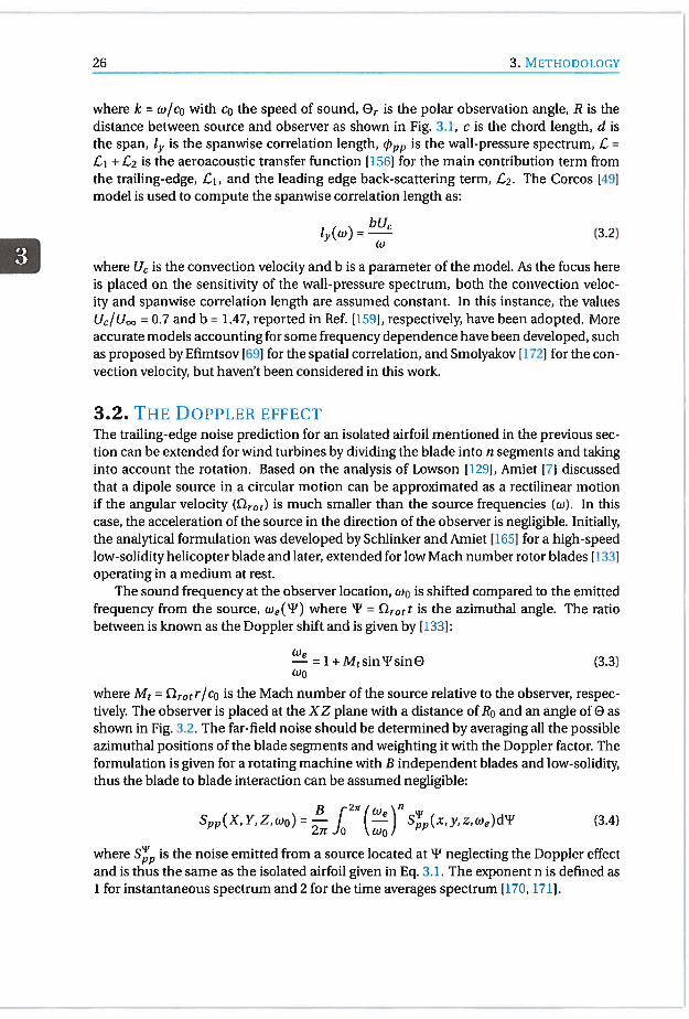
gence for the low frequencies, and also due to the mesh size and numerical schemes thatare required for the high frequencies in particular. Therefore, this section presents models which are governed by the boundary layer profiles that can be obtained from RANSsimulations. The first two approaches are based on fitting the experimental wall pressure spectra rescaled with the boundary layer variables. The last one is based on reconstructing the wall-pressure fluctuations by integrating the Poisson equation for pressure.Semi-empirical wall-pressure spectrum (WPS) models often have the form [39, 98, 1191:

pp a(w*)b

- [j(w*)c+d]e+[fRgw*]

The shape of the spectra is modified through the parameters a—h given in Eq. (3.5). Theoverall amplitude of the spectra is altered by a. The slopes corresponding to differentfrequencies are adjusted by the parameters b, c, e and h. The parameter b determinesthe slope at low frequencies. The overlap region is modified by the parameters b, c and e.The high slope region is adapted by the parameters b and h. The onset of the transitionbetween the overlap and high frequency region is adjusted by the parameters f and gin combination with timescale ratio R. The location of the low-frequency maxima isweakly dependent on the parameter d. Lastly, the parameter i is 1.0 for all except theRozenberg model. For that model, a constant of 4.76 is introduced when the boundarylayer thickness is replaced by the displacement thickness by assuming A 6/6* 8. Thescaling factor for the spectrum is and for the frequency it is w.

In this work six different semi-empirical wall-pressure spectrum models are investigated: Goody, Rozenberg, Catlett, Kamruzzaman, Hu & Herr and Lee. The parametersand the scaling factors are summarized in Table 3.1 excepted for the Lee model that is anextension of the Rozenberg model. In the following section, the governing variables andthe spectral behavior of each model are discussed.

3.4.1. SEMI-EMPIRICAL MODELSGoody model

The Goody model extends the overlap region by introducing the timescale ratio, RT,which accounts for Reynolds number effects for Zero Pressure Gradient (ZPG) boundarylayers. The wall-pressure spectrum is scaled by mixed variables: 6 is the boundary layerthickness, Ue is the velocity at the edge of the boundary layer, and is the wall shearstress. The timescale ratio is defined as the ratio of the outer time scale to the inner timescale, RT = (o/U)/(v/u) where u is the friction velocity and v is the kinematic viscosity. The frequency is scaled by S/Ue. The spectrum has a slope of w2 at low frequencies. Itdecays with a slope of w°7 at mid-frequencies and w at high frequencies. This modelis accurate over a wide range of Reynolds numbers [1011. Furthermore, it is consideredas a basis for the Adverse Pressure Gradient (APG) wall-pressure spectrum models.

Rozenberg model

Rozenberg et al. [1591 proposed a wall-pressure model based on the Goody model byconsidering the variations between ZPG and APG flows. Firstly, the scaling factor forboth spectrum and frequency was replaced by the displacement thickness, 6*, instead

30 3. METHODOLOGY

of the boundary layer thickness, 6, since the former was found to be more accurate. Secondly, the scaling for the pressure fluctuations was changed to the maximum shear stressalong the normal distance, T7nax. In addition, to characterize the effect of theAPG, threeparameters are defined: Zagarola-Smits’ parameter [2001, A = 6/8*, the Clauser equilibrium parameter [46], /3T = (8/r)(dp/dx), where 8 is the momentum thickness, andthe Coles wake parameter [47], Fl. It is found that Zagarola-Smits’ defect law provides abetter collapse than the defect law and exhibits an auto-similarity of the velocity profilefor the outer region. Thus, Zagarola-Smits’ parameter, A = 8/6*, is chosen as a drivingparameter for the APG. f3 is used to quantify the local pressure gradient even though thetested boundary layers were non-equilibrium flows. 11 represents the large-eddy structures in the outer region of the turbulent boundary layer. Coles [47] modified the law ofthe wall with an additional wake parameter as:

+ 1 + 214 .

it — ln(y ) + C + — sin —) (3.6)K K \261

where ii = u/UT = YUr/V, K = 0.41 is the von Karman constant, C 5.1 and the Coles’wake parameter, 11, can be obtained by solving the following implicit equation numerically:

KUe 6*Ue211 —ln(Il + 1) —ln(————) —KC—lnK. (3.7)

UT V

Alternatively, LI can be estimated through an empirical formula proposed by Durbin andReif [67]:

LI 0.8(/3 + 0.5)1. (3.8)

It is pointed out that A and LI are influenced by the boundary layer history whereasf3 is a local parameter. As A decreases, the amplitude of the spectrum increases at midand high frequencies and decreases for low frequencies. f3 and 14 are correlated; whenthey increase, the peak amplitude gets higher and the slope of the overlap region getssteeper.

Catlett model

Catlett et al. [39] developed a new empirical approach for APG boundary layers based onthe Goody model by testing three different trailing edge configurations for a flat plate.The scaling factor for the wall-pressure spectrum and frequency are kept the same asGoody’s model. Similar to the Rozenberg model, the local pressure gradient is defined inthe form of the Clauser equilibrium parameter, f3,. However, the length and pressure arescaled with outer boundary layer variables, fJ, where q 0.5pU is the dynamicpressure and Uo is the local free-stream velocity. They found that when the parametersa and c — h are plotted as a function of Po,Reo or J3 H, they fit into a power-law function. A is the Rotta-Clauser parameter [46, 157] defIned as A = 6*,/(2/Cf), Cf rw/q

(ö,A)Ue *is the skin friction coefficient, Re6=

are the Reynolds numbers and H = 6 /8is the shape factor. Contrary to all the semi-empirical models investigated in this study,the boundary layer thickness is deduced by a percentage of the turbulent kinetic energy,

3.4. WALL PRESSURE SPECTRUM MODELS 31

TKE(y=ô) 0.0002U [164].

Katnruzzainan model

Kamruzzaman et al. [110] modified the Goody and Rozenberg models to present a newwall-pressure spectrum model for the airfoil trailing-edge noise prediction. Variousairfoils with different angles of attack and Reynolds number were used to develop themodel. They perform the same scaling factors for the normalization of the wall-pressurespectra and frequency as in the Rozenberg model except that T,nax is replaced with ru,.The spectral amplitude for all frequencies are modulated by the parameter a which is acombination of LI and H while the rest of the parameters are kept constant by fitting

2

to the experimental data. Furthermore, the definition of RT is modified to RT =

to account for the boundary layer loading effects. The parameter is obtained by acurve-fit proposed by Nash [136]:

G = + 1.81— 1.7, where H (i—

with =. (3.9)

Finally, the Coles wake parameter is computed from Eq. 3.8 which is the same way as inthe Rozenberg model.

Hu & Herr model

Ru and Herr [981 developed a new model based on the Goody model by measuring theunsteady pressure fluctuations on a flat plate. The adverse and favorable pressure gradients were created by a NACAOO12 airfoil set at different angles of attack. Contrary to theother models, they argued that the scaling factors for the wall-pressure spectra, Ø’j and

the frequency, are more suitable for APG flow. As a consequence, a better agreementis observed when the timescale ratio, RT, is replaced by ReT. Moreover, it is acknowledged that the boundary layer profile is a main driving parameter for the wall-pressurefluctuations. Thus, the spectral slope at medium frequencies is characterized by theshape factor H, rather than the form of a Clauser’s equilibrium parameter fl, which failsat accounting for rapid pressure gradient alterations. Lastly, it is explained that the lowfrequency slope, w2, does not hold in the case of non-frozen turbulence and is bettermodelled using b = 1.0. They also pointed out that the turbulence-turbulence term inthe Poisson equation gains importance over the mean-shear source term and exhibits aplateau at low frequencies.

Lee model

Lee and Villaescusa [119] suggested an extended version of the Rozenberg model to provide an accurate prediction for extensive applications. For convenience, the scaling factor used in the normalization of the spectra, T,flax is replaced by r while keeping theother scaling parameters the same. They found that the Rozenberg model performs anearly transition from the overlap region to high frequency region. Furthermore, at highfrequencies for zero and low pressure gradient flows, a rapid decay rate is observed. Toovercome this, the parameter 12 is modified as follows:

32 3. METIoDoioGy

h min(5.35, 0.139 + 3.1043/3, 19/v”) + 7, (3.10)

and if h is equal to 12.35, the following expression is used:

hmin(3,19/\/)+7. (3.11)

The Rozenberg model exhibits higher amplitudes at low and mid-frequencies forlow pressure gradient flows. Thus, the parameter d at the denominator is modified asd = max(1.0,1.5d) if f3 < 0.5 to alter the trend. It should be noted that the parameter d in the calculation of the parameter a is kept as in the original model. Lastly,a correction is suggested for the parameter a to adjust the amplitudes for high /3 asa* =max(1,(0.25/3c—0.52)a).

Tab

le3.

1:T

hep

aram

eter

san

dsc

alin

gfa

ctor

sfo

rth

ese

mi-

empir

ical

mo

del

s

Go

od

yR

oze

nb

erg

Cat

lett

Kam

ruzz

aman

I-lu

&H

err

a13.

0[2

.82

A(6

.13

A°7

5+

d)]

e7

98

R3

1-1

O.7

+3

.00.4

5[1

.75(H

2I)

m+

15]

(81.o

o4d

+2.1

54)-

b-7

x[4

.2(-

AJ_

)+1]

m=

0.5

(y’1

)°3

b2.

02.

02.

02.

01.

0

c0.

750.

752

0.9

(fl6

Re°

5)2

76

+0

.91

21.

637

1.5

(1.1

691

n(H

)+

0.6

42

)16

d0.

54

76

()°7

5[0

.375e—

11

0.3

28(/

Re3

5)°

310+

0397

0.27

10

5810

Re01

-135

e3.

73

.7+

l.5[

—1

.93

(5R

e°5

)°6

28

+3

.87

22.

471.1

3/(

1.1

691

n(H

)+0.

642)

0.6

f1.

18.

8—

2.5

7(i

oR

e°5

)°2

24

+2

.19

1.15

_2/7

7.64

5

g-0

.57

-0.5

73

8.1

(/3

II_

05

)2h

1—

0.54

24-2

/7-0

.411

h7

min

(3,l

9//

)+

70

.79

7(j

Re3

5)°

°72

4+

7.3

I07

6

i1.

04.

761.

01.

01.

0

RR

TR

RT

RT

R

ç*

T,ô

/Ue

yn

ax

ö*

/Ue

T,6

/Ue

Tô

*/U

eq

26/u

1

WW

6/U

e0)

6*/U

0)6/

U5

0)6*

/Uw

O/U

o

-c ci c,j -c C.) 0 0 ci

1T

he

para

mete

ra

inth

eL

eeand

Vil

laes

cusa

[119

]m

od

elis

rep

laced

by

a*

34 3. Mrri-ioDoLooy

3.4.2. THE INTEGRAL MODEL

As an alternative to the previously described models, the following statistical model proposed by Panton and Linebarger [142] and later by Remmler et al. [154] is also used in thepresent paper. The incompressible Navier-Stokes equation is reformulated in the formof a Poisson equation for pressure to express the wall-pressure fluctuations beneath theturbulent boundary layer. With the assumption of statistically stationary and homogeneous flow in the streamwise and spanwise directions, the Poisson equation can besolved by using a Green’s function technique as:

2

(k1) 8p2 fff )2 S22(y,,w)‘

‘ dyddk (3.12)

where k %/k + k, U1 is the streamwise velocity and y is the wall normal direction.The energy spectrum of the vertical velocity fluctuations S22 is given as:

S22(y, 9,w)=

A2 ff R22 cos(a,(w) i) cos(a,) did, (3.13)

where i4 is the root mean square of the wall-normal velocity fluctuations, A is the integral length scale and a is the scale anisotropy factor which is the ratio of streamwise tospanwise turbulent length scales which is defined by Remmler et al. [154[ as:

3, k,o<1

a= 0, 1k1o5. (3.14)

1, kö<5

The velocity correlation function R22 is modeled according to Panton & Linebarger 1142]:

R22= 1—?2

e_2 (3.15)2\/f2÷j2

with r2 1j2 + r Non-dimensionalisation of the integration coordinates and the wavenumbers was performed by the integrallength scale, fj rt/A, k1 = k1Aand= (y—9)/A.The five dimensional integration in Eq. (3.12) is performed with a Monte Carlo methodusing importance sampling for enhancing convergence to reduce the computationalcost of the numerical integration of the fivefold integration. The reader is referred toRef. 11541 for further details on the Monte Carlo method.

The vertical velocity fluctuations cannot be obtained from the k—w turbulence modelwhich assumes isotropic turbulence. However, the measurements performed by KIebanoff 11131 for a zero pressure gradient boundary layer demonstrate that the veloc

—2ity fluctuation components, u’s, are not constant fractions of 2k. He proposed an

—2anisotropy factor for each component as f3 = u’1/(2k) where /3 is a non-universalparameter depending on the types of boundary-layer flows. As a first approximation,Remmier et al. 1154] proposed to use an anisotropy factor, which is obtained from a flat

3.5. COUPLING WITH CFD 35

plate boundary layer simulation using a Reynolds stress transport model in which thevelocity fluctuation components can be obtained directly.

Panton & Linebarger have specified the length scale, A, as 1.5 times the Prandtl mixing length, 1m’ A = 1.5lm which can be calculated as = LC, where L is the turbulencelength scale. C,7 is a turbulence model constant and was chosen as 1.9 for the k—c2SST [154]. The turbulence length scale, L, can be computed directly from the numericalsimulations in which the turbulence model provides the turbulent kinetic energy andturbulent dissipation rate as:

k312L=C_L. (3.16)

C

C1 is given as 0.09 and the turbulent dissipation, e, is calculated as c k . w.The crucial parameters for the semi-empirical models are the boundary layer thick

ness, 6, the boundary layer edge velocity, Lie, the wall-shear stress, Tw and the friction velocity, UT, which are the only variables in the Goody model. All the other non-dimensional parameters can be derived from the boundary layer variables. In addition,the Rozenberg, Kamruzzaman and Lee models used the Coles’ wake parameter, LI andthe Clauser equilibrium parameter, f3. Similarly, Catlett used a form of the Clauser parameter in their model. The appeal of these approaches is that only the velocity profile normal to the surface is needed. In addition to the velocity profile, the Panton &Linebarger model requires the turbulent kinetic energy and the specific dissipation profiles.

3.5. CouPIiiG WITH CFDThe wall-pressure models require a description of the turbulent boundary layer at thetrailing-edge which can be obtained by a panel method coupled with an integral bound-ary layer formulation as in the XFOIL software [611 or through a HANS simulation. Thefirst approach is found to be rapid and accurate at low Reynolds number [1671 and hasbeen used for wind turbine [22, 1861 trailing-edge noise applications. The global turbulent boundary layer variables (except the boundary layer thickness) can be obtaineddirectly as an output, and the boundary layer thickness and velocity profile along thewall-normal direction are approximated. In contrast, the latter approach provides theturbulent boundary layer profile in which the required variables can be derived from

HANS simulations. Since the prediction of the wall-pressure spectrum depends on theturbulent boundary layer just upstream of the trailing edge, it is important to correctlysimulate the physics and determine the adequate mesh resolution for the turbulencemodel to increase the accuracy [441. This numerical procedure has proved to be successful for low-speed fan applications [154, 1591. In this thesis, this approach is furtherextended for wind turbine applications.

The coupling between the BANS simulation and the acoustic prediction is given inFig. 3.4. After performing the BANS simulations, the BATMAN (Broadband And TonalModels for Airfoil Noise) in-house code of the von Karman Institute for Fluid Dynamics(VKI) is used to perform the acoustic part. The BATMAN code is based on MATLAB andPython routines. The VisualizationToolkit [1661 libraries in Python are used to read,

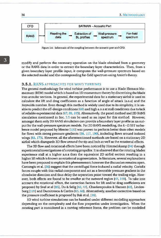
36 3. METHoiooG’

CFD

NSH

BATMAN —Acoustic Part

Reading the Extraction of Wall-pressure Far-fielddata BL profiles : spectrum spectrum

Figure 3.4: Schematic of the coupling between the acoustic part and CFD.

modify and perform the necessary operation on the blade obtained from a geometryor the HANS data in order to extract the boundary layer characteristics. Then, from agiven boundary layer profile input, it computes the wall-pressure spectrum based onthe selected model and the corresponding far-field spectrum using Amiet’s theory.

3.5.1. RANS APPROACHES FOR WIND TURBINES

The general methodology for wind turbine performance is to use a Blade Element Momentum (BEM) model which is based on 1D momentum theory by discretizing the bladeinto annular sections. In general, the experimental data for a stationary airfoil is used tocalculate the lift and drag coefficients as a function of angle of attack (a.o.a) and theReynolds number. Even though this method is widely used due to its simplicity, it is unable to predict the off-design conditions 1681 and high a.o.a at stall conditions due to lackof reliable experimental data [87, 89, 185]. Alternatively, the panel method and 2D HANSsimulation mentioned in Sec. 3.5 can be used as an input for this method. However,amongst them only 2D HANS simulation can provide a boundary layer profile as an output for the wall-pressure spectrum models. For 2D HANS modelling, the k—c2 SST turbulence model proposed by Menter 1130] was proven to perform better than other modelsfor flows with strong pressure gradients [38, 117, 1901, including flows around isolatedwings [83, 1731. However, all the aforementioned methods are based on a stationary 2Dairfoil which disregards 3D flow around the tip and hub as well as the rotational effects.

The 3D flow and rotational effects have been noticed by Himmelskamp 194] throughexperimental investigations of a rotating propeller. It is observed that the rotating bladesexperience stall at a higher a.o.a than the equivalent 2D airfoil section resulting in ahigher lift which is known as rotational augmentation. In literature, several explanationshave been proposed to explain this phenomenon; however the discussion remains open.Carcangiu et al. [36] suggest that the centrifugal force induced a radial velocity. Coriolisforces couple with this radial component and act as a favorable pressure gradient in thechordwise direction and thus delay the separation point toward the trailing edge. However, both effects are found to be smaller at the outward region 143, 168]. To take intoaccount the rotational effect, the correction factors for lift and/or drag coefficients areproposed by Snel at al [85], Du & Selig [62, 63], Chaviaropoulos & Hansen [43], Lindenburg [1261 and Dumitrescu & Cardos [65, 66]. Alternatively, another correction based onthe pressure coefficient is proposed by Bak et al. [16].

3D wind turbine simulations can be handled under different modelling approachesdepending on the complexity and the flow properties under investigation. When therotating part is considered in a moving reference frame, the problem can be modelled

3.5. CouiiNG WITI-I CFD 37

as a steady-state problem. In this case, the moving parts can be solved in the rotatingreference frame by accounting for the centrifugal and Coriolis force source terms in themomentum equation. A Single Reference Frame (SRF) can be used if the entire computational domain rotates with the same speed with respect to a specified single axis.The Multiple Reference Frame (MRF) method is a steady-state approach in which thecell zones can be assigned at different rotational or translational speeds. The movingcell zones are solved in the rotating frame while the stationary cell zones are solved inthe stationary frame. In this approach, the flow information passes directly betweenthe subdomains which means that the relative motion between the moving zone withrespect to the adjacent domain is not considered. This method is also referred to as a‘frozen rotor approach”since the rotor is fixed in a specific location and the instantaneous flow field is observed. When the unsteady interaction between the moving andstationary part is of interest, a Sliding Mesh Method (SMM) can be implemented to capture the transient phenomena. The sliding mesh method is the most accurate amongstthese methods to simulate the multiple rotating reference frames, but it is demanding interms of computational cost [187]. Since the mean boundary layer profiles are neededin order to predict the wall-pressure spectrum, the MRF method has been chosen for the3D simulation.

For the turbulence model, as it is stated by Tachos et al. [180], the k — !2 SST turbulence model performs better than the Spalart-Alimaras [175] and RenormalizationGroup (RNG) k-c 11991 models for the NREL Phase VI rotor blade. Moreover, it hasbeen found in the literature that this model has been used extensively for wind turbines [81, 135, 143, 174].

It should be also taken into consideration that the RANS models are based on theBoussinesq approximation, which assumes isotropic flow even though the flow is mostlyanisotropic. Moreover, the viscosity within the boundary layer is over-predicted, whichtends to artificially delay separation.

3.5.2. 3D AND 2D RANS APPROACH FOR FAR-FIELD NOISE OF A WIND TUR

BINE

This section describes the coupling of RANS simulations and the far-field acoustic calculation. As a first step, the 3D simulation of a wind turbine will be performed with thek — c2 SST turbulence model using the MRF method. Next, the RANS data will be read bythe BATMAN in-house code. Then, the blade will be divided into equidistant strips andthe midspan of each section will be identified. The boundary layer profiles; the mean axial velocity, the turbulence kinetic energy and the specific dissipation rate are extractedat a specified point near the trailing-edge normal to the blade surface on the midspan location. By obtaining the boundary layer profiles, the wall-pressure spectrum canbe predicted at each strip location. For the far-field noise prediction, each strip is approximated as a flat plate to obtain linearized strips, then the acoustic transfer functionis calculated at the observer position. This will be performed for sufficient azimuthalpositions for each strip locations and averaged.

The drawback of this approach is the time it takes to obtain a reliable simulationand the post-processing of a 3D geometry. To this end, a 2D approach similar to BEMis proposed as a simplification. The 3D and rotational effects are neglected in this case,

38 3. METHoDoLoGY

which leads to obtain isoradius blade cuts, Therefore, from the geometry file, the bladecan be divided into several isoradius cuts to obtain the same relative velocity for the 2Dsimulation. However, as the blade cut is performed at a certain radius from the center,the obtained blade cuts are not planar but rather a curved surface. To obtain a planarsurface, the unwrapping process shown in Fig. 3.5 is applied. At each strip location (n),the blade is cut with a cylinder having a radius of R,. The angle a,,7 is calculated foreach point (in), x,, yin,?, Z011, which is obtained by the intersection of the cylinder withblade. Then, each new point location is found and projected on to the yz plane for 2Dsimulations (x,fl,1, = (R,,a,011, z,n,,,O)).

y y

Strip,, , Yn,n, Zmn Strip,, ,‘nn Z,’nn

a,,,,,

_________

—

- a/t’1

X<ççZy1

(“1‘“ Z,flfl

O)

Figure 3.5: Unfolding procedure for an isoradius cut.

After performing the 2D simulations for each strip location, the boundary layer proifies are extracted at the same region as the 3D simulations and are imposed on the BAT-MAN code as boundary layer proffles to follow the same procedure. The flowcharts ofthese two processes have been demonstrated for 3 strips in Fig. 3.6. It should be notedthat all processes shown in the flowchart for the 2D approach are done by the geometryifie, so only a 2D mesh and 2D simulations are needed for the number of strips. Theresults from these 2D simulations are then fed into the BATMAN code to perform thefar-field noise prediction at a given observer point.

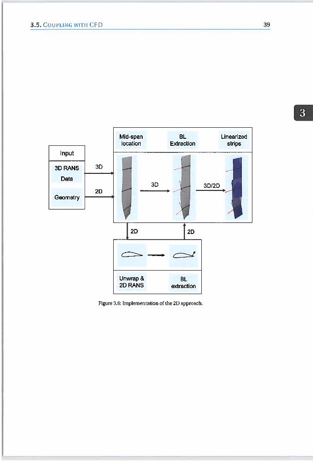
3.5. COuPLING \Ifl’H CFD 39

Mid-span BL Linearized

___________

location Extraction strips

Input

3DRANS 3DI —

Data I I

2D3D 3D/2D

Geometry

2D 2D

_

I

Unwrap & BL2D RANS extraction

Figure 3.6: Implementation of the 2D approach.

4ACCURACY AND MESH SENSITIVITY

OF RANS-BASED TRAILING-EDGE

NOISE PREDICTION USING AMIET’S

THEORY FOR AN ISOLATED AIRFOIL

Airfoil self-noise is generated by the interaction of an airfoil with the turbulence that develops within its boundary layers and wake. According to Brooks et al. [31], it constitutesthe dominant noise producing mechanism in applications such as low-speed coolingfans [45], wind turbines [20, 1381 or high-lift devices [147].

Following the framework developed by Amiet [8], the mechanism of trailing edgenoise generation can be represented as a scattering problem, where the convected wall-pressure disturbances associated with the turbulent boundary layer radiate acousticwaves to the far-field when they approach the trailing-edge discontinuity In this model,the prediction of the acoustic field is based on a statistical description of the pressurefield underneath the incoming turbulent boundary layer. To this end, two families ofmethods can be distinguished: i) based on a solution of the Poisson equation by integrating velocity statistics over the boundary layer thickness, or ii) directly addressing wall-pressure statistics through ad-hoc empirical models calibrated on experimentaldatabases. In both cases, a Reynolds-Averaged Navier-Stokes (RANS) simulation of theflow field around the airfoil is in principle sufficient to provide the necessary input data,as long as the near-wall boundary layer is resolved well enough. An objective of thiswork is the comparison of the accuracy and numerical robustness that can be obtainedby both approaches, depending on the near-wall resolution of the RANS model.

The commonly recommended wall-normal resolution for a correct modelling ofboundary layer flows is < 1 for the first mesh node adjacent to the wall, where

= Y UT/V is the non-dimensional wall-normal coordinate with v the kinematic viscosity and UT \/7 the friction velocity based on the wall friction r and fluid density

41

4. ACCURACY AND MESH SENSITIVITY OF RANS-BA5ED TRAILING-EDGE NOISE

42 PREDICTION USING A4IET’s THEORY FOR AN ISOLATED AIRFOIL

p. However, to authors’ knowledge, the influence of the grid near-wall resolution on thedetermination of the wall-pressure spectrum models and far-field predictions have notbeen addressed in the literature, despite the practical importance of the issue in terms ofcost vs. accurac Furthermore, the wall-pressure model is reconstructed near the trailing edge (x/c> 0.98) at where the applicability of some of the models is questionable.This chapter addresses this aspect. Two paths are followed to estimate the wall-pressurespectrum near the trailing edge, on the basis of HANS data. The first approach consistsin re-scaling non-dimensional wall-pressure models which are the Goody, Rozenberg,Kamruzzaman and Lee models described in the previous chapter. The second approachuses the Panton and Linebarger 1142] model based on an integration of the Poisson equation, also described in Chapter 3. It involves a priori less restrictive assumptions aboutthe flow and should thus be more generally applicable. The wall-pressure spectra predicted by those methods with different grid resolutions are then used to predict the far-field noise prediction with Arniet’s theory.

4.1. NuMERIcAL SIMULATIONS

4.1.1. AIRFOIL CONFIGURATIONS

The two following airfoils, chosen from the BANC benchmark database [92], have beenconsidered in this study: NACAOO12 and DU96-W-180 with a sharp trailing edge. TheNACAOO12 is a zero cambered airfoil with 12% maximum thickness. The DU96-W-180airfoil has a maximum thickness of 18% and has a 25% maximum camber at the 36.4%position of the chord. The dimensions and the operating conditions are given in Table 4.1. The NACA airfoil is tripped at 0.065% of the chord, both on the suction sideand the pressure side, and is measured in the Laminar Wind Tunnel (LWT) of the University of Stuttgart 1911. For the DU96-W-180 airfoil, a trip strip is located at x/c 0.05for the suction side and x/c 0.1 for the pressure side 1911. The NACAOO12 experimental database includes the pressure distribution along the airfoil, velocity profiles, wall-pressure spectra and far-field noise measurements, while the DU96-W-180 database isrestricted to far-field acoustic measurements [911. The far-field spectra are computed atan observer distance of r = 1 m and for a wetted span of b = 1 m. 8r is the angle from thelistener with the origin along the streamwise direction.

Table 4.1: Airfoil configuration

Airfoil a.o.a c Re U p° m - rn/s kg/rn3

NACAOO12 0 0.4 1.5x106 56 1.181

DU96-W-180 4 0.3 1.13 x 106 60 1.164

4.2. MESH SENSITIVITY 43

4.1.2. CoMPuTATIoNAL SETUPSteady two dimensional (2D) RANS simulations are performed with the open source CFDsolver OpenFOAM 4.0 using the k—cl SST turbulence model proposed by Menter [130].The simulations are performed assuming turbulent flow along the full chord of the airfoils. A turbulence intensity of 0.1%, is applied at the inlet of the computational domain.The boundary conditions at the inlet are chosen as Dirichlet boundary conditions for allthe variables except the pressure for which the gradient is set to zero. At the airfoil surface, low-Reynolds number wall functions are used for the kinetic energy k, the turbulentviscosity v and the specific dissipation 2. A no-slip condition is applied for the velocityand the pressure gradient is set to zero. At the outlet,the gradients of all variables are setto zero expect for the pressure that is imposed to be zero. Symmetric boundary conditions are applied at the top and bottom boundaries. The incompressible solver simple-Foam is used to perform the simulations. Second order accurate schemes are used withthe under-relaxation of 0.7 for U, k, 2 and 0.3 for p.

4.2. MESH SENSITIVITYThe mesh is created with ANSYS ICEM. The mesh topology is based on the C-Grid type,which is here combined with an H-Grid, to optimize the skewness of the cells. Thegrowth rate is chosen as 1.05 and the number of hexahedral cells can be found in Table 4.2 depending on the mesh refinement.

The domain size convergence is tested with two different configurations. The firstconfiguration has a lOc length in the wall normal direction, 5c and lOc in the upstreamand downstream directions, respectively. The second configuration is increased to 20cin the wall normal direction, lOc and 30c in the upstream and downstream directions,respectively. It is verified that the two domain sizes yield the same pressure coefficientalong the airfoil and vertical velocity profile at x/c 0.99. As a result, the domain withlOc lateral extent has been retained for the further calculations.

The generally recommended wall normal spacing for wall bounded flows is < ,

i.e. well within the laminar sublayer. In this study different values starting from thecoarsest, = 10, to the finest, y4 < 1, are investigated for both airfoils as listed in Table 4.2. It can be seen that for the DU96-W-180 airfoil, having 0.35 on the suctionside does not ensure yet the condition < 1 on the pressure side, so that the finest meshhas been further refined to obtain <1 on both sides.

4.2.1. PRESSURE DISTRIBUTION AND BOUNDARY LAYER PROFILESAs mentioned in Section 3.4, the semi-empirical models require as input only the meanvelocity profile, and the streamwise pressure gradient for those models that account forits effect, whereas the Panton & Linebarger model necessitates also turbulence profiles.Both pressure distributions along the airfoil and boundary layer statistics have thus beenconsidered in the analysis below.

NACAOO12 RESULTS

The pressure coefficient along the NACAOO12 airfoil and the boundary layer profiles atx/c = 0.99 are investigated with respect to different wall normal spacings given in Table 4.2. The pressure distribution given in Fig. 4.1(a) appears insensitive with respect to

4. AccuRAcYAND MESH SENSITIVITY OF RANS-BASED TRAILING-EDGE NOISE

44 PREDICTION USING AMIEr ‘S THEORY FOR AN ISOLATED AIRFOIL

Table 4.2: WaIl normal spacing for two airfoils

Mrfoils Ay/cx i03 Number of cells Mi y Max.atx/c=0.99%

Suction side Pressure side

0.6 81876 4 21 11.31

NACAOO12 0.3 93368 2.92 13.5 5.34

0.05 125192 0.5 2.5 0.82

0.01 154364 0.1 0.5 0.17

2 76363 7 37.5 10 23.2

0.8 89636 3 22 4.2 13.8

DU96-W-180 0.4 100867 1.11 15 1.53 8.14

0.1 126392 0.13 5 0.35 2.1

0.01 173358 0.019 0.5 0.04 0.2

the different grid refinements. A good match with the experiment [91] is obtained exceptfor the transition region, x/c 0.05, which is expected as the present simulations assumefully turbulent flows. The velocity profile shown in Fig. 4.1(b) is also pretty much insensitive to the mesh refinement and matches fairly well the experimental data too [93]. Themaximum turbulent kinetic energy (Fig. 4.1(c)) is seen to vary more significantly, furthermore its convergence cannot be definitely concluded considering its non-monotonousevolution with respect to the grid spacing. The difference between the finest mesh to thecoarsest mesh is found to be 11%. The specific dissipation profile (Fig. 4.1(d)) exhibitsinsensitivity to the mesh resolution from the wall till y/c 0.01. Above this value, smallchanges are observed with respect to different grid sizes.

DU96-W-180 RESULTS

The results obtained for the DU96-W-180 airfoil with the mesh refinements given in Table 4.2 are shown in Fig. 4.2. As for the NACAOO12 airfoil, the pressure distribution appears insensitive with respect to the grid size (Fig. 4.2(a)). The profiles of mean axial velocity, turbulent kinetic energy and specific dissipation extracted at x/c 0.99 are givenin Fig. 4.2(b),(c) and (d), respectively. It appears that the results obtained for the pressure side are less mesh-dependent than for the suction side, with the exception of thespecific dissipation. The suction side boundary layer tends to thicken with the mesh refinement, while the pressure side boundary layer thickness remains overall unaffected.It is also observed that the coarsest mesh is unable to capture the velocity profile belowy/c < 0.002. Consistently with the NACAOO12 results, the turbulent kinetic energy profileexhibits a somewhat larger mesh sensitivity than the other quantities, with a maximumat the suction side that increases and shifts slightly upwards with finer meshes. The difference between the coarsest and the finest grids is around 16%. The kinetic energy profile on the pressure side is less affected. In contrast with the other quantities, the specificdissipation profile displays a slightly larger sensitivity on the pressure side than on the

4.2. MEsH SENSITIVITY 45

Figure 4.1: Pressure coefficient along the airfoil and non-dimensional boundary layer profiles at x/ C = 0.99from the leading edge with different grid sizes for the NAA0012 airfoil; suction side; (—), y 5 - 4,

1 (— — ), y 0.2 1—’—) and experiments (°) from Ref. [921.

suction side (Fig. 4.2(d)).

4.2.2. CALcuLATIoN OF THE GLOBAL VARIABLESIn Section 3.4, it is noted that the commonly used approach to determine the boundarylayer thickness, ö, is to find the location where the boundary layer edge velocity, Ue, is0.99% of the free-stream velocity U5 = 0.99 U. However, this approach is not applicablein the presence of the adverse pressure gradient due to the fact that the free stream velocity, U, does not converge to a certain value. In the following, three different approachesfor defining the boundary layer thickness are presented:

1. Herr et a1. 1921 proposed to determine the boundary layer thickness at the inflection point.

2. the boundary layer thickness is defined as the distance where the turbulent kineticenergy is equal to TKE(o) 0.0002U [39].

0.5

0

C)

ci>.

0.2 0.4 0.6xIc [-]

(a) Pressure coefficient.

ci>

ci>

u/u... [-1

(b) Mean axial velocity.

0.05

0.04

0.03

00 0.002 0.004kIU [-]

(C) Turbulent kinetic energy.

‘io° 10’ 10 1O’ 102c/Q [-I

(d) Specific dissipation.

3. the boundary layer thickness is defined as the position at which the total pressure

4. ACCURACY AND MESH SENSITIVITY OF RANS-BAsED TRAILING-EDGE NOISE

46 PREDICTION USING AMIEr’s THEORY FOR AN ISOLATED AIRFOIL

°-°5F

0.5 0.04

0 : 0.03

001 C046081

xlc [-] ufu_

(a) Pressure coefficient. (b) Mean axial velocity.

0 0.004 0.008 100 10’ 102 100 io i0k,/U [-] Qc/lJ, [-]

(C) Turbulent kinetic energy. (d) Specific dissipation.

Figure 4.2: Pressure coefficient along the airfoil and non-dimensional boundary layer profiles at x/c = 0.99from the leading edge with different grid sizes for the DU96-W-180 airfoil; y 23 1—), y .. 14 (- -

8 (— —‘), y 2 ( . ...), y 0.2 C ) and (line-symbols: suction side, line: pressure side).

is 99% of the maximum total pressure.

The boundary layer profile normal to the surface is extracted at x/c 0.99 from theleading edge. Figure 4.3 represents the position of the boundary layer thickness and thecorresponding edge-velocity for NACAOO12 at 00 angle of attack with three different approaches mentioned previously. The inflection point method in Fig. 4.3(a), where thesecond derivative of the streamwise velocity with respect to the wall-normal distancechanges the sign, proposed by Herr et al. [92] is challenging since the second derivative is noisy and over-estimated the value which is not shown in the Fig. 4.3. Thus, theinflection point is determined from the minimum value of the first derivative. The second approach is to assign the boundary layer thickness from the kinetic energy whereTKE(ö) = 0.0002U [39] (Fig. 4.3(b)). This method is more straightforward since theright-hand side of the equation is a known value. The last method considered in thispaper is to locate 8 at which the total pressure is 99% of the maximum total pressure.Even though the approach seems similar to the commonly used method, U5/U 0.99,it guarantees that the total pressure becomes constant above the boundary layer thick-

4.2. MEsFI SENSITIVITY

0.04

0.03

0.02

0.01

0.4 0.6u/u [-]

(a) First method.

47

Figure 4.3: Determination of the boundary layer thickness and the corresponding boundary layer edge velocitywith three different methods for the NACAOO12 airfoil at 00 angle of attack obtained at x/c = 0.99 from theleading edge.

ness (Fig. 4.3(c)). The values obtained using each methods are given in Table 4.3. Thenext step is to investigate the sensitivity of the semi-empirical methods to the boundarylayer thickness and the boundary layer edge velocity obtained from three different approaches. The momentum thickness, e, and displacement thickness, ö, are computedfor each method. The friction velocity, u, and Coles’ wake parameter, LI, are found byfitting the velocity boundary layer to the law of the wake.

The effect of the different boundary layer thicknesses and edge velocities on the wall-pressure spectra predicted by the Goody, Rozenberg and Catlett models are shown inFig. 4.4, and are compared with experimental data. The other models are found to beinsensitive to these parameters and not presented in the paper. It is observed that theGoody and Catlett models exhibit a similar behavior. The models are insensitive to theboundary layer parameters at moderate and high frequency whereas 1 dB deviations occurs at low-frequencies. On the contrary, the Rozenberg model is sensitive to the boundary layer parameters for the low frequencies. From the point of maximum of, up to thehighest frequency a deviation of up to 2 dB occurs. The other models mentioned in Sec

C [-10 0.2 0.4 Rot 0.6 0.8

0406081u/u. [-]

(C) Third method.

0.02 C-)

0.4 0.6u/u= [-1

(b) Second method.

484. ACCURACY AND MESH SENSITIVITY OF RANS-BA5ED TRAILING-EDGE NOISE

PREDICTION USING AMIET’S THEORY FOR AN ISOLATED AIRFOIL

Table 4.3: Boundary layer thickness and boundary layer edge velocity obtained by three different methods forthe NACAOO12 airfoil at 00 angle of attack obtained at x/c = 0.99.

Nz

0

e

Method 6/c Ue/U 6*/c 8/c

1 0.0252 0.9231 0.0058 0.0035

2 0.0235 0.9202 0.0057 0.0034

3 0.0229 0.9186 0.0057 0.0034

Figure 4.4: Wall-pressure spectra prediction by different models at x/c = 0.99 from the leading edge for theNACAOO12 airfoil at 00 angle of attack; Rozenberg (—), Goody (—), Catlett (—) models and experimentaldata from LWT F) 192]; l method (— —

2nd method ( —) and 3 method C—).

tion 3.4 are disregarded since they do not exhibit any sensitivity to the boundary layerparameters. When the scaling parameters for the spectrum and the frequency are considered, Goody and Catlett models are the only ones who used the same scaling. Thiscould be a possible explanation of their similar behavior even though their parametrization is completely different. For the Rozenberg model, the driving parameter for thetrend is mainly A which appears only in this model. Overall, it is observed that the firstmethod over-predicts the boundary layer parameters and under-estimates the high frequency part for the Rozenberg model. The drawback of the Catlett et al. [39] method isthat when the simulations are performed by a two-equation turbulence model, it is notalways possible to acquire the turbulent kinetic energy, k accurately. Thus, in terms ofease and direct comparison to experimental data, it is suggested that the boundary layerthickness obtained by the total pressure method is more suitable. Consequently, thismethod has been applied to all the results presented herein after. Furthermore, the experimental data is dominated by the background noise after 15 kHz, thus the frequencieshigher than this will be neglected for the following parts.

5 10 15 20f [kHz]

4.2, MESH SENSITIVITY 49

The other discrepancy found in Section 3.4 regarding the semi-empirical models isthe determination of H and /3c. These parameters are only in the Rozenberg and Kamruzzaman models. In both models, H is calculated from Eq. 3.8 whereas f3 is calculatedfrom Eq. 3.9 for the Kamruzzaman model. However, in the present study, IS is obtainedfrom solving Eq. 3.7 implicitly as well as finding the best fit with the law of the wakewhereas the 13c value is calculated directly from the definition of the Clauser’s equilibrium parameter, which is the same method as the Rozenberg model. The correspondingvalues for two models are given in Table 4.4 and compared with the experimental datain Fig. 4.5.

Table 4.4: Values of H and f3c obtained from different equations.

Models Fl f-3c H

(O/r)(dp/dx) Eq.3.7 Eq.3.9 Eq.3.8

Rozenberg -

5.2832 2.2931 2.9834Kamruzzaman 5.1670

In the general form of the wall-pressure spectrum given in Eq. 3.5, the parameter a,which alters the amplitude of the spectrum, is driven by Fl for the Rozenberg model while11 and tic for the Kamruzzaman model. The corresponding values are given in Table 3.1.Figure 4.5(a) shows an increment of 1 dB over the whole range of the spectrum whenthe Fl value is increased by 30%. For the Kamruzzaman model, even though 13c valueis reduced by 2%, which should result in a decrease on the amplitude of the spectra,an increment of less than 1 dB is observed since the increment of H is more dominant.Furthermore, the comparison with the experimental data reveals that the amplitude forthe low and mid frequencies are captured better with the newly calculated variables.However, the higher frequency part is over-estimated for both models. In conclusion,this analysis demonstrates that there is not a certain method that gives the most accurateprediction. Depending on the definition of the variable the spectrum of the amplitudechanges around ±1 dB. The wall-pressure spectra presented herein after are calculatedby the methods considered in the current study which provide better predictions for thehigher frequencies. The comparison of the models with respect to the experimental datais investigated in the Sec. 4.2.3.

4.2.3. PREDIcTIoN OF THE WALL-PRESSURE SPECTRA AND FAR-FIELDTRAILING EDGE NOISE

Based on the above results, the impact of the mesh resolution on the noise obtainedby means of the semi-empirical models is evaluated for the DU96-W-180 airfoil only,since the NACAOO12 pressure distribution and mean velocity profiles are fairly meshinsensitive. In contrast, the boundary layer turbulent kinetic energy proffles, used as input for the Panton & Linebarger model, showed more significant discrepancies for boththe NACAOO12 and DU96-W-180 airfoils.

50

4. AccuicY AND MESH SENSITIVITY OF RANS-BAsED TRAIL1NG-EDGE NO1SE

PREDICTION USING AMIEf’s THEORY FOR AN ISOLATED AIRFOIL

N

e

(a) Rozenberg model. (b) Kamruzzaman model.

Figure 4.5: The comparison of the wall-pressure spectra which is calculated by different definition of fir andH; (—) is calculated by H obtained from the Eq. 3.7 and fir from (O/rju)(dp/dx); (— — -) is calculated byH obtained from the Eq. 3.8 for both models and flc is calculated from Eq. 3.9 for only Kamruzzaman model;experimental data from LWT(0) [92].

NACAOO12 RESULTS OBTAINED USING PANTON & LINEBARGER INTEGRAL APPItOACI-l

The wall-pressure spectra predicted by the Panton arid Linebarger fl42] model is shownin Fig. 4.6(a) where the dimensionless frequency is obtained by the values in Table 4.5.

Only the suction side results are displayed for this symmetric airfoil at 00 angle of attack. It has been verified that the variations that can be observed for dimensionlessfrequencies below 0.7 are due to an insufficient convergence of the Monte-Carlo integration leading to uncertainties of around 3 dB, and the results below that frequency willnot be further discussed.

It is observed that the fluctuation amplitude obtained with y 11 deviates fromthe others by about 3 dB for middle frequencies. The difference decreases for higher

f[kHzj f[kHz]

NII

80

75

70

65

60

55

I

-J

W6/Ue 1]345

kc [-]

(a) \Vall-pressure spectrum at xJc 0.99. (b) Far-field third-octave noise spectrum.Figure 4.6: Wall-pressure spectra prediction by the Panton and Linebarger [142] model and the correspondingfar.lnleld noise prediction with different grid sizes: y 11 (—1. j’ 5 (— — 1, y 1 ( —. I, y 0.2 (— ‘—).

4.2. MESH SENSITIVITY 51

frequencies. Logically, the same observation can be made for the 1/3-octave band far-field trailing edge noise prediction. This must be attributed to the differences observedin the turbulent kinetic energy profiles in Fig. 4.2(c). It can be concluded that y < 5yields a convergence towards the finest mesh sound spectra within 1 dB.

NACAOO12 RESUIIS OBTAINED USING TI-IL SEMI-EMPIRICAl. AND INTEGRAL APPROACHES

In terms of absolute validation, the wall-pressure spectra predicted by the seven models depicted in this paper for the NACAOO12 airfoil, and the corresponding 1/3-octaveband far-field noise spectra, are compared in Fig. 4.7 with experimental data obtainedin DLR’s Acoustic Wind-Tunnel Braunschweig (AWB), JAG Laminar Wind Tunnel (LWT)and UF Aeroacoustic Flow Facility (UFAFF) 1921. Considering the wall-pressure spectrafirstly, it can be first observed that the ZPG model of Goody performs poorly as shown inFig. 4.7(a), which is sensible considering the non-negligible APG near the trailing edge ofthis airfoil. Models including an APG correction proved to yield much better agreementwith experimental data except for the Catlett and Herr & Hu models. They share a common point; both of them performed their experiments on a flat-plate where a APG flow iscreated with trailing-edge sections 1391 or a rotational airfoil [98] and obtained satisfactory results. Even though, they compared their model with Rozenberg’s model, they havenot performed any predictions for airfoil flows. There, it can be deduced that these models are unrepresentative for airfoils. The Rozenberg model demonstrates a good matchfor the high frequencies whereas the maximum amplitude is underestimated.

a a80 a

— - —‘S

.:--.-.‘.N.

\ a70

65

wIU0 [-[

(a) Wall-pressure spectrum at x/c = 0.99. (b) Far-field third-octave noise spectrum.

Pigure 4.7: Far-field noise prediction by different wall-pressure spectrum models for the NACAOO12; Goody), Rozenberg (—), Catlett (- . —), Kamruzzaman (— ‘— ), Herr & Ho (— —), Lee ( ), Panton &

Linebarger (- - .) models and experimental data from LWT H AWB (0), UFAFF (A).

Kamrazzumari model, which is developed by considering airfoil flows, performs better compared to the previous models. The model under-predicted below wö*/Ue <0.7and over-predicts above that range. When the formalization is considered, all the parameters are constant except the parameter a which is a function of H and /3 and onlyregulates the spectrum amplitude. Thus, increasing the amplitude by changing thoseparameters will perform a better match for the peak region whereas worsen the higherfrequencies. Furthermore, it is observed that by reducing the parameter d, the peak

kc [-]

4. AccuoAcYND MESH SENSITIVITY OF RANS-BAsED TRAILiNG-EDGE NOISE

52 PREDICTION USING ArvITET’S THEORY FOR AN ISOLATED AIRFOIL

point of the spectra shifts to the lower frequencies as well as the amplitude of the fre

quencies below the peak point increases which is lacking in this model. Thus, it can beconcluded that this model provides a good prediction around ±3 dB above the middlefrequency range regarding to its simplicity. The Lee model provides results identical tothose of the Rozenberg model in this case. The reason as stated in Sec. 3.4 is that onlythe a, d and 12 parameters are modified to take into account the aforementioned issues.These parameters are a function of f3 or RT. In this airfoil case, a and d parametersgive the same value as in the Rozenberg model and the value of the h parameter is onlyslightly different (see Table 4.5 for the values.). The statistical model proposed by Panton& Linebarger, captures the trend for all the cases, however, under-predicts around 3 dB.The possible reason for the under-estimation is due to the anisotropy factor applied forthe wall-normal velocity fluctuations which are obtained from a flat-plate. However, forAPG flows, it is expected to be higher.

Table 4.5: Boundary layer parameters.

NACAOO12 QO

U5/U 0.9186

6/c 0.02296*/c 0.0057

0/c 0.0034

u/U00 0.0277

A 4.02

RT 28.80

H 2.2931

I3 5.2832

H 1.676

A 0.2056

About the far-field noise predictions, the results shown in Fig. 4.7(b) confirm that theGoody, Catlett and Herr & Hu models model yield a poor agreement with experimental data. A good match is obtained using the Rozenberg and Lee models and the UAFFand AWB dataset for the highest frequencies kc > 60. The Kamruzzaman model performs well for the middle range but over-predicts the highest frequencies by about 2 dB.Comparison with theAWB data shows that the model of Panton & Linebarger gives goodresults below kc < 20 but under-predicts slightly the higher frequencies. A possible improvement could be the reconstruction of the streamwise velocity fluctuations with ananisotropy factor accounting for pressure gradient effects.

DU96-W-180 RESULTS

The variables required by the semi-empirical models have been determined processing the boundary layer profile data shown in Fig. 4.2, to yield the values given in Ta-

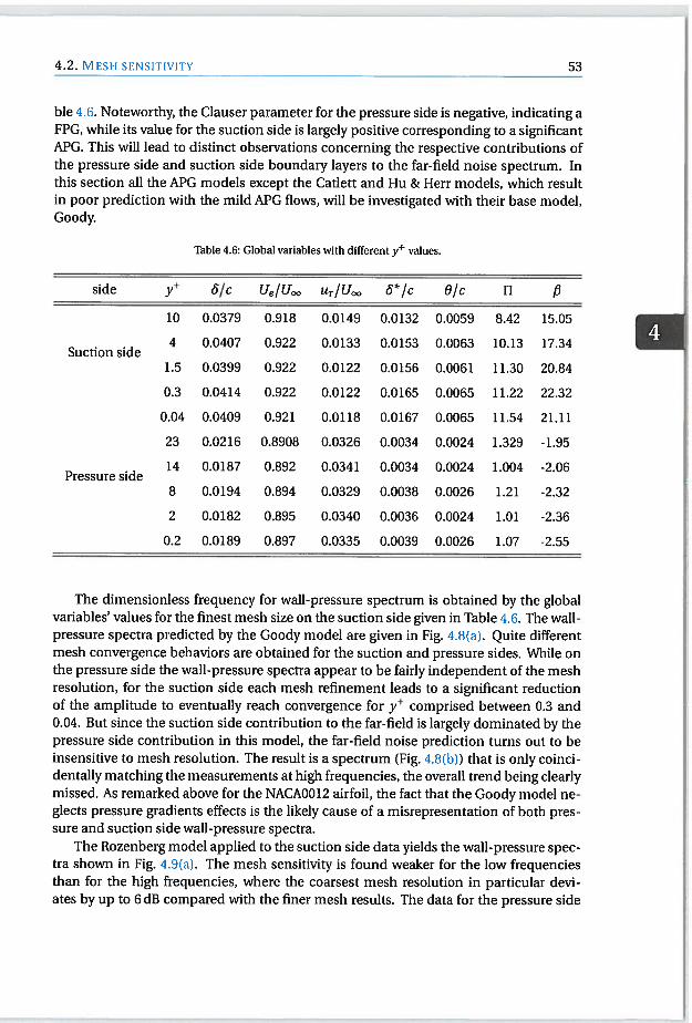
4.2. MESH SENSITIVITY 53

ble 4.6. Noteworthy, the Clauser parameter for the pressure side is negative, indicating aFPG, while its value for the suction side is largely positive corresponding to a significantAPG. This will lead to distinct observations concerning the respective contributions ofthe pressure side and suction side boundary layers to the far-field noise spectrum. Inthis section all the APG models except the Catlett and Ru & Herr models, which resultin poor prediction with the mild APG flows, will be investigated with their base model,Goody.

Table 46: Global variables with different yf values.

side y 6/c Lie/tic,0 U/U,c, 6*/c 0/c Fl /3

10 0.0379 0.918 0.0149 0.0132 0.0059 8.42 15.05

. 4 0.0407 0.922 0.0133 0.0153 0.0063 10.13 17.34Suction side

1.5 0.0399 0.922 0.0122 0.0156 0.0061 11.30 20.84

0.3 0.0414 0.922 0.0122 0.0165 0.0065 11.22 22.32

0.04 0.0409 0.921 0.0118 0.0167 0.0065 11.54 21.11

23 0.0216 0.8908 0.0326 0.0034 0.0024 1.329 -1.95

. 14 0.0187 0.892 0.0341 0.0034 0.0024 1.004 -2.06Pressure side

8 0.0194 0.894 0.0329 0.0038 0.0026 1.21 -2.32

2 0.0182 0.895 0.0340 0.0036 0.0024 1.01 -2.36

0.2 0.0189 0.897 0.0335 0.0039 0.0026 1.07 -2.55

The dimensionless frequency for wall-pressure spectrum is obtained by the globalvariables’ values for the finest mesh size on the suction side given in Table 4.6. The wall-pressure spectra predicted by the Goody model are given in Fig. 4.8(a). Quite differentmesh convergence behaviors are obtained for the suction and pressure sides. While onthe pressure side the wall-pressure spectra appear to be fairly independent of the meshresolution, for the suction side each mesh refinement leads to a significant reductionof the amplitude to eventually reach convergence for comprised between 0.3 and0.04. But since the suction side contribution to the far-field is largely dominated by thepressure side contribution in this model, the far-field noise prediction turns out to beinsensitive to mesh resolution. The result is a spectrum (Fig. 4.8(b)) that is only coincidentally matching the measurements at high frequencies, the overall trend being clearlymissed. As remarked above for the NACAOO12 airfoil, the fact that the Goody model neglects pressure gradients effects is the likely cause of a misrepresentation of both pressure and suction side wall-pressure spectra.

The Rozenberg model applied to the suction side data yields the wall-pressure spectra shown in Fig. 4.9(a). The mesh sensitivity is found weaker for the low frequenciesthan for the high frequencies, where the coarsest mesh resolution in particular deviates by up to 6 dB compared with the finer mesh results. The data for the pressure side

4. AccuoAcv AND MESH SENSITIVITY OF RANS-BA5ED TRAILING-EDGE NOISE

54 PREDICTION USING AMIET’s THEORY FOR AN ISOLATED AIRFOIL

80 00

600

— 0

(I)6/Ue [] kc [-I

(a) Wall-pressure spectrum at x/c = 0.99. (b) Far-field third-octave noise spectrum.

Figure 4.8: WaIl-pressure spectra prediction by the Goody [791 model and corresponding the far-field noiseprediction with different grid sizes for the DU96-W-180. Pressure side (plain): j’ 23 (), y 14 ( —

y8(--),y2(”-),y0.2( );suctionside(.): y 10(—),y 4(- --),j’1.5(--),0.3 ( ) y 0.04 ( ); experiments [92]: 0

have not been used in the Rozenberg model following the recommendations of Rozenberg et ad. [159] themselves, who advised against using their model for FPG. However,the Goody model has been presumed to be applicable to the pressure side, owing to themoderate FPG that is reported in Table 4.6. Consequently, the far-field noise predictionshown in Fig. 4.9(b) has been obtained using the Rozenberg model for the suction sideand the Goody model for the pressure side. The result is a spectrum exhibiting higherlevels at low frequencies than using the Goody model for both sides, thereby reducingsomewhat the gap with the experimental data. The spectrum a high frequencies beingdominated by the pressure side contribution, it is similar to that shown in Fig. 4.8(b). Thecombined model remains overall unable to capture both the trend and the amplitude ofthe measured sound field. In terms of mesh dependency, it is observed that the resultsare insensitive to the mesh size even though the coarsest mesh on the pressure side isaround y 23.

The wall-pressure spectra obtained using the Kamruzzaman model in Fig. 4.10(a)exhibit variations of about 4 dB between the coarsest and the finest grid sizes for thesuction side, converging within 2 dB for yf less than 4. A smaller sensitivity is foundfor the pressure side, especially at high frequencies. Interestingly, for the suction sidea mesh refinement induces an increase of the low-frequency levels and a reduction ofthe high-frequency content with little impact around w6*/U 1.2, while the effect ismore uniformly distributed for the pressure side. The combination of the pressure andsuction side sensitivities yields a far-field noise prediction in Fig. 4.10(b) that is fairlymesh-independent for frequencies above kc> 10, where the model provides also fairagreement with experimental data. The levels are under-predicted by about 3 dB at lowerfrequencies.

The Lee model performs similarly to the Rozenberg model in terms of mesh sensitivity (Fig. 4.11(a)), but gives significantly higher levels (up to B dB) as a result of modifyingthe A parameter. This model is also inapplicable to FPG flows so that the Goody model is

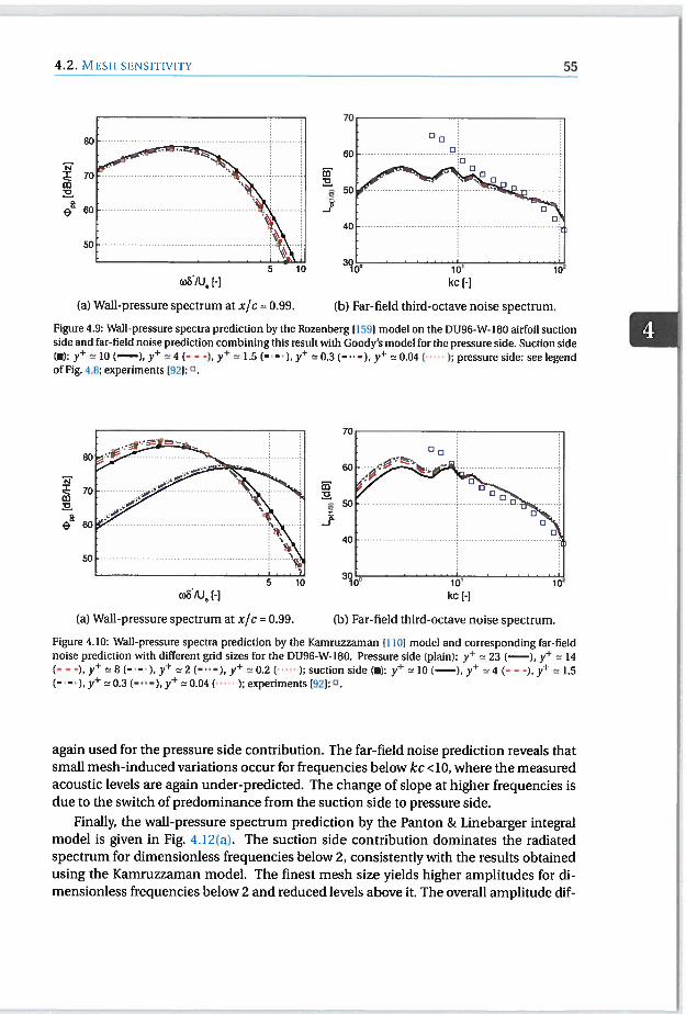
4.2. MEsFI SENSITIVITY 55

NxCO

e

again used for the pressure side contribution. The far-field noise prediction reveals thatsmall mesh-induced variations occur for frequencies below kc <10, where the measuredacoustic levels are again under-predicted. The change of slope at higher frequencies isdue to the switch of predominance from the suction side to pressure side.

Finally, the wall-pressure spectrum prediction by the Panton & Linebarger integralmodel is given in Fig. 4.12(a). The suction side contribution dominates the radiatedspectrum for dimensionless frequencies below 2, consistently with the results obtainedusing the Kamruzzaman model. The finest mesh size yields higher amplitudes for dimensionless frequencies below 2 and reduced levels above it. The overall amplitude dif

CO

‘2

-J

60

50

40

CD

PS

tai/U0 I-I..i0 10’ 1o

cikc [-I

(a) \‘Vall-pressure spectrum at x/c = 0.99. (b) Far-field third-octave noise spectrum.

Figure 4.9: Wall-pressure spectra prediction by the Rozenberg [159] model on the DU96-W-180 airfoil suctionside and far-field noise prediction combining this result with Goody’s model for the pressure side. Suction side(I): y 10 (), y 4 ( - ), y 1.5 (), y 0.3 (— ‘-), y 0.04 ( ); pressure side: see legendof Fig. 4.8; experiments 1921:0.

NzCO0

e

(a) Wall-pressure spectrum at x/c = 0.99. (b) Far-field third-octave noise spectrum.

Figure 4.10: Wall-pressure spectra prediction by the Kamruzzaman 11101 model and corresponding far-fieldnoise prediction with different grid sizes for the DU96-W-180. Pressure side (plain): y 23 1—), y 14(---)y B(--’),y 2(-”-),y 0.2( );suctionside (.): y 10(—),y 4 t---)y 1.5

), y 0.3 ( . . ), y 0.041 . ‘ ); experiments 192]: D

ro6 /U 1-] kc [-]

4. AccuRAcY AND MESH SENSITIVITY OF RANS-BAsED TRAILING-EDGE NOISE

56 PREDICTION USING AMIET’s THEORY FOR AN ISOLATED AIRFOIL

kc [-]

(b) Far-field noise prediction.

10 10

(06/Ue []

(a) Wall-pressure spectra prediction.

Figure 4.11: WaIl-pressure spectra prediction by the Lee 11191 model on the DU96-W-180 airfoil suction sideand far-field noise prediction combining this result with Goody’s model for the pressure side. Suction side (.):

10 C—), y 4 (- - -), y 1.5 (——), y 0.3 (— —), y 0.04 C ); pressure side: see legend ofFig. 4.8; experiments [921:0.

ference remains around 2 dB between the finest and the coarsest mesh. For the pressureside, the difference between the coarsest and the other meshes increases more significandy above wö* /U5 >2. This could be related to the discrepancies mentioned above forthe velocity and specific dissipation profiles (Fig. 4.2(a) and 4.2(b)). The far-field noise

prediction shown in Fig. 4.12(b) shows that the stronger pressure side variability has

a significant effect on the predicted sound spectrum, unexpectedly providing a better

agreement with experiments for the coarsest mesh. Apart from this - likely coincidental- effect, the mesh-related variability of the predicted spectra remains within 2 dB. Theoverall comparison with the measured sound spectrum is overall good, with substantialimprovetnents at the lowest frequencies compared with the semi-empirical models.

4.3. EFFECT OF THE PROBE LOCATION ALONG THE AIRFOIL

In the previous section, the far-field noise are performed by the wall-pressure spectrawhich are obtained from the boundary layer profiles extracted at the x/c 0.99. However, it is observed that the Rozenberg and Lee models are inapplicable at the locationwhere the boundary layer is exposed to a FPG flow. The focus of this section is to investigate the effect of the pressure gradient on the wall-pressure spectrum and the far-fieldnoise prediction along the airfoil chord by extracting the boundary layer profiles fromdifferent probe locations, x/c 0.9 till 0.99, for the DU96-W-180 airfoil. Later, the wall-pressure spectra models will be computed for each probe location to investigate the sensitivity on the local quantities. The velocity proffle in Fig. 4.13 shows that the APG has asignificant effect on the suction side. Hence, the value of integral boundary layer parameters (ö, ö and 6) and the wake parameters (11, /3) increase and the other parameters:U5 and UT decrease as shown in Tab. 4.7. For the pressure side, the APG is present untily/c 0.05 which can be deduced from the pressure coefficient in Fig. 4.2(a). After thatlocation, there is a favorable pressure gradient, /3 <0 (see Tab. 4.7). The turbulent kinetic

80

N

70

60

50

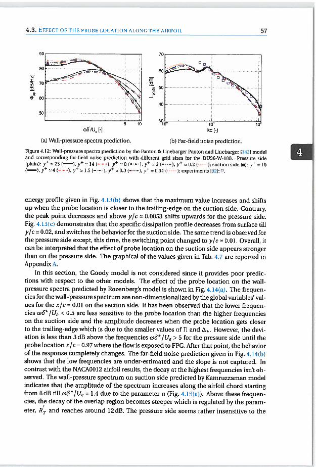
4.3. EFFEcT OF THE PROBE LOCATION ALONG THE AIRFOIL 57

NI

(b) Far-field noise prediction.

Figure 4.12: WaIl-pressure spectra prediction by the Panton & Linebarger Panton and Linebarger [142] modeland corresponding far-field noise prediction with different grid sizes for the DU96-W-180. Pressure side(plain): y 23 (—), y 14 C- — ), yf 8 y 2 (....), y 0.2 ( ); suction side (a): y 10(—), y 4 ( •) y 1.5 (..) y 0.3 (.‘—), y 0.04 ( ); experiments 1021:0.

energy profile given in Fig. 4.13(b) shows that the maximum value increases and shiftsup when the probe location is closer to the trailing-edge on the suction side. Contrary,the peak point decreases and above y/c 0.0053 shifts upwards for the pressure side.Fig. 4.13(c) demonstrates that the specific dissipation profile decreases from surface tilly/c 0.02, and switches the behavior for the suction side. The same trend is observed forthe pressure side except, this time, the switching point changed to y/c 0.01. Overall, itcan be interpreted that the effect of probe location on the suction side appears strongerthan on the pressure side. The graphical of the values given in Tab. 4.7 are reported inAppendixA.

In this section, the Goody model is not considered since it provides poor predictions with respect to the other models. The effect of the probe location on the wail-pressure spectra predicted by Rozenberg’s model is shown in Fig. 4.14(a). The frequencies for the wall-pressure spectrum are non-dimensionalized by the global variables’ values for the x/c = 0.01 on the section side. It has been observed that the lower frequencies wô*/Ue < 0.5 are less sensitive to the probe location than the higher frequencieson the suction side and the amplitude decreases when the probe location gets closerto the trailing-edge which is due to the smaller values of Fl and A. However, the deviation is less than 3dB above the frequencies wö*/Ue > 5 for the pressure side until theprobe location x/c 0.97 where the flow is exposed to FPG. After that point, the behaviorof the response completely changes. The far-field noise prediction given in Fig. 4.14(b)shows that the low frequencies are under-estimated and the slope is not captured. Incontrast with the NACAOO12 airfoil results, the decay at the highest frequencies isn’t observed. The wall-pressure spectrum on suction side predicted by Kamruzzaman modelindicates that the amplitude of the spectrum increases along the airfoil chord startingfrom 8dB till w6*/Ue 1.4 due to the parameter a (Fig. 4.15(a)). Above these frequencies, the decay of the overlap region becomes steeper which is regulated by the parameter, RT and reaches around 12 dB. The pressure side seems rather insensitive to the

W6IUe [] kc [1

(a) Wall-pressure spectra prediction.

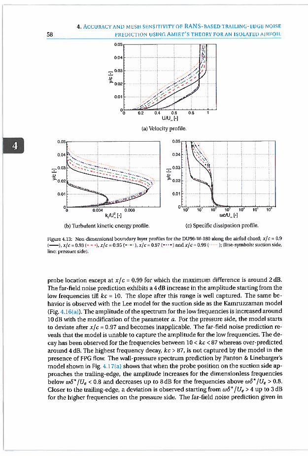
4. ACCURACY AND MESH SENSITIVITY OF RANS-BAsED TRAILING-EDGE NOISE

58 PREDICTION USING AMIET’s THEORY FOR AN ISOLATED AIRFOIL

C-)>.

Figure 4.13: Non-dimensional boundary layer profiles for Ihe DU9B-W-180 along the airfoil chord; x/c = 0.9

(—), x/c = 0.93 (- - 1 x/c = 0.95 (— — ), x/c = 0.97 (— . —) and x/c = 0.99 ( ); (line-symbols: suction side,

line: pressure side).

probe location except at x/c = 0.99 for which the maximum difference is around 2 dB.

The far-field noise prediction exhibits a 4 dB increase in the amplitude starting from the

low frequencies till kc 10. The slope after this range is well captured. The same behavior is observed with the Lee model for the suction side as the Kamruzzaman model(Fig. 4.16(a)). The amplitude of the spectrum for the low frequencies is increased around10 dB with the modification of the parameter a. For the pressure side, the model startsto deviate after x/c 0.97 and becomes inapplicable. The far-field noise prediction reveals that the model is unable to capture the amplitude for the low frequencies. The decay has been observed for the frequencies between 10 < kc < 87 whereas over-predictedaround 4dB. The highest frequency decay kc > 87, is not captured by the model in thepresence of FPG flow. The wall-pressure spectrum prediction by Panton & Linebarger’smodel shown in Fig. 4.17(a) shows that when the probe position on the suction side approaches the trailing-edge, the amplitude increases for the dimensionless frequenciesbelow wö*/Ue <0.8 and decreases up to 8dB for the frequencies above wö*/Ue > 0.8.Closer to the trailing-edge, a deviation is observed starting from wö/U5 > 4 up to 3dBfor the higher frequencies on the pressure side. The far-field noise prediction given in

u/u= [-]

(a) Velocity profile.

(b) Turbulent kinetic energy profile. (c) Specific dissipation profile.

4.3. EFFECT OF TFIE PROBE LOCATION ALONG THE AIRFOIL 59

Table 4.7: Global variables with respect to probe location.

x/c side ö/c Ue/Uo., U/Uco 6*/c 0/c fT /3

0 1SS 0.0296 0.976 0.0210 0.0098 0.0049 5.10 8.16

PS 0.0179 0.894 0.0313 0.0040 0.0025 1.57 0.48

0.07SS 0.0329 0.956 0.0183 0.0115 0.0054 6.34 11.22

PS 0.0184 0.888 0.0311 0.0042 0.0026 1.53 0.48

0 05ss 0.0357 0.944 0.0163 0.0130 0.0058 7.55 14.07

PS 0.0188 0.888 0.0312 0.0042 0.0027 1.48 0.27

0.03ss 0.0376 0.93 0.0141 0.0146 0.0062 9.12 18.48

PS 0.0189 0.890 0.0318 0.0042 0.0027 1.35 -0.55

001SS 0.0409 0.921 0.0118 0.0167 0.0065 11.54 21.11

PS 0.0189 0.897 0.0335 0.0039 0.0026 1.07 -2.55

Fig. 4.17(b) exhibits that a deviation of 4dB above kc> 10 can be obtained with differentprobe positions.

-.100 10’ 10

(a) Wall-pressure spectra prediction. (b) Far-field noise prediction.

Figure 4.14: Wall-pressure spectrum predicted by the Rozenberg 11591 model and corresponding the far-fieldnoise prediction on the DU96-W-180 airfoil varying extraction position along the chord; x/c = 0.9 (—),x/c = 0.93 (- — -), x/c = 0.95 (— —‘), x/c 0.97 (—‘ —) and x/c = 0.99 ( ); (line-symbols: Suction side, line:pressure side).

N

w6/U0 [-1 kc [-]

4. AccunAcY AND MESH SENSITIVITY OF RANS-BA5ED TRAILING-EDGE NOISE

60 PREDICTION USING AMIET’s TFIEORY FOR AN ISOLATED AIRFOIL

NI

It

:/flDDDD\\

3So

4.4. CoNcLusioNsThis study focuses on the effect of grid spacing on the wall-pressure spectra and far-fieldnoise predicted for NACAOO12 and DU96-W-180 airfoils using Amiet’s linearized airfoiltheory. Two categories of wall-pressure spectrum models have been investigated. Firstly,semi-empirical models have been considered, where the wall-pressure spectrum is rescaled with the mixed boundary layer variables, thus only requiring the boundary layervelocity profile (and for some models the pressure gradient) at the trailing edge. In thiscategory, the models of Goody (assuming ZPG), and Rozenberg, Kamruzzaman, Catlett,Ru & Herr, Lee (accounting for APG effects) are compared. Secondly, an integral model

80

.\\

50

-J

kc [-110

ceo/U0

(a) Wall-pressure spectra prediction. (b) Far-field noise prediction.

Figure 4.15: The wall-pressure spectrum predicted by the Kamruzzaman [1101 model and corresponding thefar-field noise prediction on the DU96-W-180 airfoil varying extraction position along the chord; x/c = 0.9(—), xJc = 0.93 (— -), x/c = 0.95 (— —, ), x/c = 0.97 (— . . —) and x/c = 0.99 ( ); (line-symbols: suction side,line: pressure side and experiments: D 1921).

NI

C

-J

5 10

U)6/U [-1

(a) Wall-pressure spectra prediction.

kc [-]

(b) Far-field noise prediction.

Figure 4.16: The wall-pressure spectrum predicted by the Lee [119] model and corresponding the far-fieldnoise prediction on the DU96-w-180 airfoil varying extration position along the chord; x/c = 0.9 (—),x/c = 0.93 (— — ), x/c = 0.95 (— —), x/c = 0.97 C—’’ —) and x/c = 0.99 ( ); (line-symbols: suction side, line:pressure side and experiments: 0 [921).

4.4. Coiictusiois 61

60

\

5O .

•l00)6/U0 [.)

(a) Wall-pressure spectra prediction. (b) Far-field noise prediction.

Figure 4.17: The wall-pressure spectrum predicted by the Panton & Linebarger [142] model and corresponding 4

the far-field noise prediction on the DU96-W-180 airfoil varying extration position along the chord; x/c = 0.9(—), x/c = 0.93 (— - ), x/c = 0.95 (— —‘), x/c = 0.97 (— . . —) and x/c = 0.99 ( .. ); (line-symbols: Suction side,line: pressure side and experiments: 0 [92]).

proposed by Panton & Linebarger is investigated, in which the wall-pressure spectrumis obtained by integrating the Poisson equation. In addition to the mean velocity profile,this model also requires the turbulent kinetic energy and specific dissipation profiles,but is on the principle more generally applicable to flows with arbitrary pressure gradients.

The grid sensitivity analysis is performed for both airfoils with different grid resolutions characterized by the value of non-dimensional wall units, at the extractionlocation x/c 0.99. For the NACAOO12 airfoil, the coarsest grid resolution is yf 10 andfor the DU96-W-180 airfoil, y 10 on the suction side and y 23 on the pressure side,and the finest grid resolution is below < 1 for both cases. It has been observed that thepressure coefficient appears insensitive to the mesh refinement for both airfoils. However, the boundary layer profiles showed different behaviors.

For the NACAOO12 airfoil, the boundary layer velocity profile at x/c 0.99 is overallinsensitive to the mesh refinement, but the turbulent kinetic energy and specific dissipation profiles displayed a larger variability. A mesh independence is achieved by the Pan-ton & Linebarger model for <5. The wall-pressure spectrum predictions by the different models show that the Goody model performs poorly with respect to the experimental data, due to the presence of APG. The Rozenberg and Lee models accounting for sucheffects proved indeed much more accurate. The Kamruzzaman model under-predictsthe low frequencies and over-predicts the higher frequencies. However, the Catlett andHu & Herr models perform poorly since they are developed for A.PG flow on a flat-plate.The Panton & Linebarger model captures the slope but under-predicts the amplitude byaround 3 dB. The same conclusion can be drawn for the far-field predictions.

For the DU96-W-180 airfoil, the velocity profile exhibit different trends with respectto the grid refinement, depending on the quantify of interest. The mesh resolution hasa larger impact on the suction side than on the pressure side, excepted for the specificdissipation proffle. In general, it has been observed that the low frequencies of the radi

kcl-l

4. AccuRAcY AND MESH SENSITIVITY OF RANS-BAsED TRAILING-EDGE NOISE

62 PREDICTION USING AMIET’s THEORY FOR AN ISOLATED AIRFOIL

ated spectrum are dominated by the suction side turbulent boundary layer, whereas the

pressure side flow is responsible for the higher frequencies. The low-frequency part ofthe predicted acoustic spectrum proves accordingly to be more mesh-dependent thanthe high-frequency part.

In more quantitative terms, it can be concluded that for the considered airfoils andflow solver, a mesh resolution below y <23 on the pressure side for the semi-empiricalmodels and <13 for the integral model is necessary to ensure the converge the radiated noise spectrum predictions. Both Rozenberg and Lee models are not used topredict the wall-pressure spectrum on the pressure side due to the presence of FPG, inwhich case the Goody model is applied. Nevertheless, a better agreement with the experimental sound spectra is observed with the Lee model. The far-field noise predictedby the Kamruzzaman model over-predicts the levels by about 3 dB for frequencies abovekc> 10. Finally, the far-field noise predicted by the Panton & Linebarger model is foundto be within ± 3 dB of the experimental data, and provides the best agreement for thelowest frequencies. It shows however a slightly larger variability than the semi-empiricalmodels.

The probe location analysis is performed with five different positions starting fromx/c = 0.9 to x/c 0.99 for the DU96-W-180 airfoil. It has been observed that the flow isexposed to an AJG flow on the suction side along the airfoil whereas on the pressure side,the flow is exposed to an APG flow until y/c = 0.95% and a FPG flow after. Moreover, thewall-pressure spectrum prediction by the models showed that the suction side is moresensitive to the probe location than the pressure side as for the boundary layer profiles.In general, the far-field noise predictions by the semi-empirical models are found to besensitive to the probe location below the frequency kc < 10.

5APPLICATION TO DIFFUSER

AUGMENTED WIND TURBINE

(DAWT)

The CAD of the DoriQi Urban Windmill shown in Fig. 5.la is provided by the Deift University of Technology (see Ref. [9] for the detailed explanation of the geometry). Thewind turbine has a radius of 0.75 m with a tip clearance of 0.015 m. The airfoil profile isa NACA22O7 along the entire blade. The chord of the blade at the hub is 0.13 m with atwist angle of 40.5° and is 0.105m with 0.3° twist at the tip. This variation is shown inFig. 5.lb.

0

F

Figure 5d (a)The geometry of the DonQi Urban Windmill; (b) The chord and twist distributions along theblade.

(a) (b)

63

64 5. APPLICATION TO DAWT

5.1. 3D NUMERICAL SIMULATIONIn this section, a 3D simulation of the DonQi Urban Windmill is performed. The MultipleReference Frame method explained as in Sec. 3 is used. The details of the computationalsetup are explained in the following parts.

5.1.1. CoMPuTATIoNAL SETUPSteady three dimensional (3D) incompressible HANS simulations of the DonQi UrbanWindmill were performed using the open source CFD solver OpenFOAM 4.0. The k — 12

SST turbulence model proposed by Menter [1301 was used as described in Chapter 4,

and assuming a turbulent flow along the blade, diffuser and hub. The inlet velocity andthe turbulence intensity were chosen as 5 m/s and 5%, respectively, which correspondsto the operating condition for the turbine [9]. The inlet velocity is uniform and the windturbine is symmetric around the rotational axis. Thus, only 120° of the full domain wasmodelled to reduce the computational effort as shown in Fig. 5.2. For the inlet and outlet, the same boundary conditions were applied as in Chapter 4 and they were placedat 8R and 7R, respectively [169] (R is the rotor radius) in front and behind the hub, respectively. A periodic boundary condition was used on the adjacent faces. The far-fieldboundary condition was assumed to be the same as the inlet and was placed at 8R toreduce interaction with the blade region [751. A closer view of the MRF zone is shownin Fig. 5.2b. The rotational speed was chosen as 12 rot = 39.84 rad/s which is found to bean ideal operating condition with a tip speed ratio of 6 as suggested by van Dorst [192].

The blade and the hub intersection with the MRF zone were considered rotating, while,the diffuser intersection with the MRF zone was considered stationary. Furthermore, acontra-rotating velocity boundary condition was exposed to the non-rotating part of thehub, the others were set to no-slip condition. The pressure gradient was set to zero andthe blended wall functions were used for the kinetic energy k, the turbulent viscosity vand the specific dissipation 12 for all the solid surfaces. The boundary conditions withthe initial values are summarized in Table 5.1.

5.1.2. MESH SENSITIVITYThe mesh was created using the ANSYS MESHING 19.0 tool by using the multizone utilitiy. The domain is subdivided into several blocks, where the outer blocks are composedof a hexadral mesh while a tetrahedral mesh is used for the inner blocks. A detail sketchof the mesh is shown in Fig. 5.3. Three different meshes were created by changing onlythe first cell thickness, while keeping the surface mesh identical. Thus, the number of thecells for each mesh configurations is sensitive to the first layer cell thickness. It can bededuced from Table 5.2 that the y value for the finest mesh is in the inner layer whereasthe medium and coarse ones are extended to the buffer layer.

To investigate the effect of mesh resolution on the blade, three strip positions arechosen: close to the hub (x/R = 0.19), at midspan (x/R = 0.55) and close to the tip (x/R0.92) which are demonstrated in Fig. 5.4. The pressure coefficient is calculated as:

- p—po1 2

(5.1)POURel

where Po and P0 are the pressure and density at the atmospheric conditions. The relative

5.1, 3D NUMERICAL SIMULATION

PERIODIC

(a) Computational domain.

.,_.____-------* Stationary patches

65

Rotating wall patches

(b) MRF region.

Figure 5.2: Computational domain.

velocity is defined as: UReI = + (c20 rt)2 depending on the strip location. Thepressure coefficient as a function of mesh resolution is shown in Fig. 5.5 at the three striplocations. It is observed that the pressure coefficient remains unchanged for the threemesh resolutions along the blade sections.

The dimensionless velocity, turbulent kinetic energy and specific dissipation boundary layer proffles extracted at x/c 0.99 from the leading edge with different mesh resolutions are given in Fig. 5.6, 5.7 and 5.8 at the three strip locations, respectively. Theaxial velocity profile shows a good match at the outer layer of the boundary layer, however, small discrepancies are observed for the inner and log-layer. It should be noted

INLET , -.

FAR-FIELD

OUTLET

STATIONARY FME /RENAME /

8R 7R

66 5. APPLIcATIoN TO DAWT

Table 5.1: Boundary conditions

U [rn/si p [Pal k [rn2/s2i Vt [rn2/si 2 [1/si

Inlet U VP=0 0.09375 - 111.8-*

Outlet VU=0 P=0 vk=0 - Vf2=0

Far-field U VP=0 0.09375 - 111.8

Blade U = 0 VP = 0 Adaptive wall-function

Diffuser T. = 0 VP = 0 Adaptive wall-function

Hub non-rotating 2rot VP = 0 Adaptive wall-function

Hub rotating = 0 VP = 0 Adaptive wall-function

Side patches cylicAMI

that even though the first layer cell is fixed during the mesh design, the first cell heightdecreases towards the trailing-edge, resulting in a less than 1 along the trailing-edgeregion for the different mesh configurations. Thus, the wall function is not employedsince the boundary layer is resolved which might explain the different behavior for eachmesh resolution. The turbulent kinetic energy profiles extracted at the same positionsshow high sensitivity to the mesh resolution. It could be observed that the difference between the mesh resolutions decreases from the hub to tip. The reason behind this maybe due to the occurrence of secondary flows at the hub. The turbulence model mightbe more sensitive to the different mesh resolution in such a flow. Furthermore, the peakpoint decreases with a finer mesh which is contrary to the outcome analysed in Sec. 4.2.Contrary to the other boundary layer profiles, the specific dissipation profiles exhibit in-

Table 5.2: Wall normal spacing for the blade

Ay/c x i03 Number of cells Mi y Max. y Average y

0.08 49 618 393 0.07 8 2.5

0.06 52 267 244 0.063 7 2

0.05 53 762 184 0.06 6 1.6

5.2. 2D ISORADIAL APPROACH 67

sensitivity to the mesh resolution. The wall-normal and spanwise velocity profiles aregiven in Appendix B. 1.

5.2. 2D ISORADIAL APPROACHThe main focus of this section is to investigate the applicability of the 2D isoradial approach which would reduce 3D computational effort in terms of both meshing and simulation cost. For this end, the isoradial methodology introduced in Sec. 3.5.1 is applied.As a first step, the effect of the nacelle and the diffuser on the flow acceleration is neglected and it is assumed that each isoradial blade section encounters the same free-stream velocity, which is applied in the previous section for three-dimensional simulations. The 2D computational setup based on this approach is explained, and followed bythe analysis on the number of strips required for a converged acoustic results by excluding the scattering due to the nacelle and diffuser, Later, in order to represent the effectof the diffuser and the nacelle on the inflow conditions due to the acceleration, a two-dimensional axisymmetric simulation is performed to obtain the inflow conditions fortwo-dimensional approach. This approach is indicated in Fig. 5.9. The flow accelerationalong the diffuser is investigated.

5.2.1. CoMPuTATIoNAL SETUPThe solver and turbulence model described in Chapter 4 were used, as well as the sameboundary conditions except for the top and bottom part of the domain. In this case,cyclic boundary conditions (cyclicAMl) were applied to take into account the periodicity. The inlet and outlet were placed 3c upstream and downstream of the airfoil. However, the distance between the top and bottom parts were modified depending on theradial position of the isoradial blade cut to satisfy the periodicity For the simplificationof the geometry, it is assumed that the axial velocity is unchanged along the axial direction. Thus, all the initial conditions given in Table 5.1 were kept the same. In addition,

Tetrahedral

Figure 5.3: The tetrahedral mesh within the hexahedral mesh.

68

Strip 3

Strip 2

Strip I

0

Figure 5.4: Three strip positions.

5. APucTo .rc DAWT

0.5

C)

-0.5

0 0.2 0.4 0.6

xIc [-)

(C) Strip 3.

Figure 5.5: Pressure coefficient along the airfoil at each strip location with different mesh resolutions; )‘ve2.5 (), y,5 2 ( - )‘ Yve 1.6 (- -1.

C)

0.4 06

x/c [-] x/c (-1

(a) Strip 1. (b) Strip 2.

0.8 1

5.2. 2D ISORADIAL APPROACH

(b) Strip 2.

Figure 5.6: Axial velocity profiles at x/c =0.99 from the leading edge at each strip location with different meshresolutions; Yve 2.5 (—), Yve 2 (— ) Y1 1.6 ( —

(b) Strip 2.

Figure 5.7: Turbulent kinetic energy profiles at x/c =0.99 from the leading edge at each strip location; Yve 2.5(), Yve 2 ( - ) Yve 1.6 ( ‘‘).

a tangential velocity was introduced due to the rotational speed of the blade which depends on the strip position, V c2rot ‘trip. A sketch shown in Fig. 5.10 illustrates theaforementioned conditions.

5.2.2. CoNvERGENcE DUE TO THE NUMBER OF STRIPSTo obtain a converged solution for the far-field spectrum, the blade is divided into 5, 10and 20 as shown in Fig. 5.11. The boundary layer profiles normal to the airfoil surfaceclose to the trailing-edge are obtained for each strip from the 2D BANS simulations. The

69

(a) Strip 1.

U/U01 [-1 U/U5ei [] U/UReI []

n IC

(c) Strip 3.

0.1

005

0.005 0.01

kt/Uei Hi

(a) Strip 1.

0.005 001k1/U []

0.005 0.01k1/U01 [-1

(c) Strip 3.

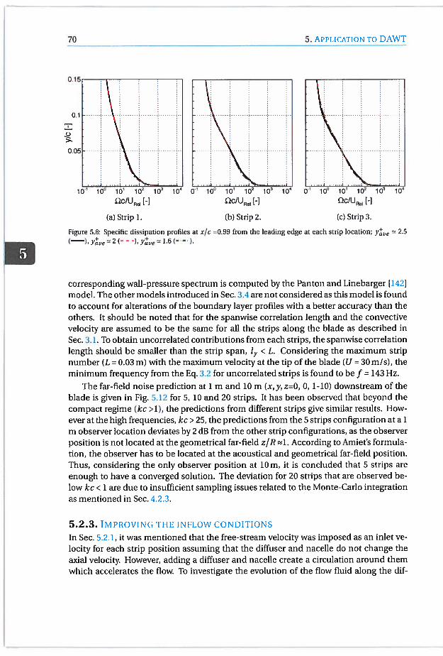
70 5. APPLIcivrI0N TO DAWT

(a) Strip 1. (b) Strip 2. (C) Strip 3.

Figure 5.8: Specific dissipation profiles at x/c =0.99 from the leading edge at each strip location; )‘ve 2.5

(), )‘ve 2 ( Yve 1.6 (- -

corresponding wall-pressure spectrum is computed by the Panton and Linebarger [142]model. The other models introduced in Sec. 3.4 are not considered as this model is foundto account for alterations of the boundary layer profiles with a better accuracy than theothers. It should be noted that for the spanwise corre]ation length and the convectivevelocity are assumed to be the same for all the strips along the blade as described inSec. 3.1. To obtain uncorrelated contributions from each strips, the spanwise correlationlength shouid be smaller than the strip span, l,, <L. Considering the maximum stripnumber (L = 0.03 m) with the maximum velocity at the tip of the blade (U 30 mIs), theminimum frequency from the Eq. 3.2 for uncorrelated strips is found to be f = 143 Hz.

The far-field noise prediction at 1 m and 10 m (x, y, z=0, 0, 1-10) downstream of theblade is given in Fig. 5.12 for 5, 10 and 20 strips. It has been observed that beyond thecompact regime (kc >1), the predictions from different strips give similar results. However at the high frequencies, kc >25, the predictions from the 5 strips configuration at a 1m observer location deviates by 2 dB from the other strip configurations, as the observerposition is not located at the geometrical far-field z/R a1. According to Amiet’s formulation, the observer has to be located at the acoustical and geometrical far-field position.Thus, considering the only observer position at 10 m, it is concluded that 5 strips areenough to have a converged solution. The deviation for 20 strips that are observed below kc < 1 are due to insufficient sampling issues related to the Monte-Carlo integrationas mentioned in Sec. 4.2.3.

5.2.3. IMPROVING THE INFLOW CONDITIONS

In Sec. 5.2.1, it was mentioned that the free-stream velocity was imposed as an inlet velocity for each strip position assuming that the diffuser and nacelle do not change theaxial velocity. However, adding a diffuser and nacelle create a circulation around themwhich accelerates the flow. To investigate the evolution of the flow fluid along the dif

c2C/UReI [-] QC/UReI [] c2c/Uoe [-1

5.2. 2D ISORADIAL APPROAC II 71

Inlet condition imposed fromthe axial location (1)

=

Strip3

Iu2 = u

‘ Strip 2

U1 =

Strip I

Inlet condition imposed fromthe axial location (2)

1!

______

Strip3

I U2

7

Str4 2

U1

Strip I

Figure 5.9: The 2D isoradial approach with the acceleration correction from a 2D axisymmetric simulation.

fuser, an axisymmetric 2D simulation was performed by neglecting the blade as shownin Fig. 5.13.

The domain size was kept the same as the 3D simulation except for the cyclic angle.In this case, the cyclic angle was 5° with a thickness of one cell in order to use the wedgeutility of OpenFoam 4.0. The same initial and boundary conditions were applied forother boundaries. A structured mesh was created with ANSYS ICEM. The wall-normalresolution is determined to be less than y <5 for both diffuser and nacelle.

The same strip locations as shown in Fig. 5.4 were used to investigate the flow acceleration along the diffuser. The dimensionless mean velocity profiles in the polar coordinate system along the diffuser are given in Fig. 5.14 where U is the axial velocity, U,.is the radial velocity, U0 tangential velocity, z corresponds to the axis of symmetry andc is the mid-chord of the blade. The origin, z/c = 0, is located on the tip of the nacellefront. The diffuser, blade, nacelle and probe locations are described in Fig. 5. 14(a. It hasbeen observed that the flow acceleration starts around z/c —1 and has its maximum

(1) (2)

ser

. - - . - . - - - -. - - - . - - - - -. - - . -— - - Strip 3

.-.-.-.-.-.— Strip2

.-.-.-.-.-.-.— ‘Ur--’ Strip 1

I NacelLe

72

INLET

(U, rotrstrip

5. AiwucArioN TO DAWT

OUTLET

Figure 5.10: Computational setup for 20 approach.

(a) 5 strips. (b) 10 strips. (C) 20 strips.

Figure 5.11: Isoradial blade Cuts of the DonQi Urban Windmill.

at the location of minimum area. Surprisingly, the first and second strips’ axial accelerations are almost identical. One might expect to observe less influence on the secondstrip due to the circulation around the diffuser and the nacelle if the distance betweenthem would be larger. Furthermore, the diffuser has a high curvature on the suctionside which leads to a greater acceleration and thus, resulting in a higher axial velocity at

TOP

BOTTOM

5.2. 2D ISORADIAL APPROACH 73

NI

0a

C/)

Figure 5.12: Far-field noise prediction at two observer locations (line:(—), 10 strips (— — -) and 20 strips ( ).

kc [-11 m, line-symbols: 10 m) with 5 strips

Figure 5.13: Computational setup for 2D axisymmetric simulation.

5. APPLICATION TO DAWT74

the midspan. The radial velocity profile shows similar results at the midspan, while thetip strip locations have a negative radial velocity component at the inlet of the diffuserwhich signify that both locations are mainly driven by the flow on the suction side ofthe diffuser. Furthermore, the absolute value of the radial component at the midspan isgreater than the strip location near the nacelle which means that the acceleration due tothe diffuser is dominant. After the minimum area location, the flow starts to deceleratefor all the strip locations. Further downstream, at z/c 8, it is observed that the radialcomponent is less pronounced for the nacelle strip location, however, the midspan andtip strip locations are still driven by the flow around the diffuser. Finally, the tangentialvelocity along each strip location is found to be zero as the rotation is neglected in thisconfiguration.

-10 -5 0 5

z/c [-]

(a) The location of the strip and probes.

: AA. •• AAA

b444**tttAA:AA AA

*

1 5

(c) Mean radial velocity.

Figure 5.14: The probe locations and mean velocity profiles along the diffuser with respect to the different striplocations; Strip 1(A), Strip 2(.) and Strip 3 (.).

5.3. CoMPARIsoN OF THE 3D AND 2D COMPUTATIONS

In this section, the comparison of the 3D and 2D simulations will be assessed in termsof the incoming velocity profile upstream of the blade, the pressure coefficient and the

8

6

4

2

*....., S..!...

.............., S..,...

A A A A A A A A A A A A A A A A A A

2

1.8

1.6

1.4

1.2

•AA

IS

S

1 5-10

zIc [-]

(b) Mean axial velocity.

0.2

_0

D-0.2

-0.4

-10 -5

zic [-I

5.3. C0MPAIus0N OF THE 3D AND 2D COMPUTATIONS 75

boundary layer profiles along each strip location. Later, the wall-pressure spectrum willbe obtained by using the models explained in Sec. 3 and the corresponding far-field noiseprediction by Amiet’s theory.

As described in the previous sections, as a first approximation for 2D computations,the diffuser and nacelle are neglected and the free-stream velocity is assumed to be uniform along the blade. However, the mean axial flow accelerates in the presence of bothdiffuser and nacelle. To consider this axial velocity acceleration on the 2D computationaldomain, three different locations are selected from the 2D axisymmetric simulations andimposed as U as shown in Fig. 5.10 with the same domain size. The first location ischosen such that the effect of the axial velocity acceleration is less than U/U < 1.15,the second location is selected before the front tip of the diffuser and the last location ischosen so that the maximum velocity could be obtained before the blade (see Fig. 5.13 atz/c = —5.0, z/c —0.5 and z/c = 0.677, respectively). The three extraction locations andcorresponding free-stream velocity values, as well as the base configuration are summarized in Table 5.3 with the same strip locations analysed in the previous sections. It willbe these three velocities at z/c [—5.0, —0.5,0.677] that will be imposed in the followingsection. It should be noted that the far-field noise predictions, the 5 strip configurationshown in Fig. 5.11(a) is used. The strip positions are numbered as Strip 1 near the hubtill Strip 5 near the tip.

Table 5.3: The extraction locations and corresponding inlet velocity boundary conditions

[-1U1 [mis] Uqc/U [-1

Strip 1 Strip 3 Strip 5 Strip] Strip 3 Strip 5

—0O 5 5 5 1 1 1

-5.0 5.5 5.4 5.2 1.1 1.08 1.04

-0.5 6.4 6.7 6.2 1.28 1.34 1.24

0.667 7 7.2 8.5 1.4 1.44 1.7

5.3.1. INLET VELOCITY PROFILESThe inlet velocity profiles obtained from the 2D simulations with different inlet velocity boundary conditions (specified in Table 5.3), and the 3D simulation are compared interms of the axial and tangential velocityin Fig. 5.15 and Fig. 5.16, respectively. The inletvelocity proffles are extracted at z/c 0.667 and plotted as a function of the azimuthalangle, 6, which is 1/3 of the domain. The comparison is performed for the same striplocations investigated in the previous sections (see Fig. 5.4) with respect to different inlet velocity profiles obtained from the 2D and 3D simulations. However, the radial inletvelocity shown in Fig. 5.17 is compared only with respect to the different strip locationssince the radial component of the velocity is neglected in 2D simulation. In all the fig-

76 5. APPLiCATiON TO DAWT

ures, the trailing-edge location is positioned at 8 = 0 rad.

As a general remark, assuming the free-stream velocity as an inlet boundary condition, the mean axial velocity profile obtained by the 2D simulation under-predictsthe inlet proffle from 3D simulation. However, imposing the maximum velocity to the2D simulation clearly over-predicts the inlet axial velocity profile when compared tothe 3D simulation. Hence, an inlet velocity between the two extreme positions mightable to reconstruct the same inlet profile from 2D simulations. Consequently, the positions at z/c —5.0 and z/c —0.5 are chosen to this end. Even though the velocityobtained at 2/c —5.0 is 1.1 times higher than the free-stream velocity, U/U = 1.1,the inlet axial profile for Strip I is over-predicted and for Strip 5 is under-predictedwhereas a good match is observed for Strip 3 in comparison to the 3D results, Finally,for Strip 5, the inlet velocity profile obtained from the 2D simulation by imposing theaxial velocity at —0.5 has a good match. The tangential mean velocity profilesnon-dimensionalized with the rotational speed shows that the profiles obtained fromthe 2D simulations perform poorly with respect to the 3D simulation. In all strip positions, the peak point of the 2D profiles is shifted to the left in comparison with the 3Dresult. The inlet radial velocity component is investigated only for 3D simulations withrespect to the different strip positions as shown in Fig. 5.17 as the 2D simulation doesnot talce into account the spanwise evaluation. When the inlet radial velocity profiles arecompared with the 2D axisymmetric simulations shown in Fig. 5.14c at z/c 0.667, it isobserved that the mean of the velocity is lower. Furthermore, the midspan location isless affected by the circulation due to the diffuser as the mean radial velocity is around

Ur/Uc,o = 0.025. It could be concluded that the presence of the blade and the rotationreduce the radial velocity component. However, it is difficult with the current studies tointerpret the magnitude of impact on the results.

5.3.2. PRESSURE DISTRIBUTION AND BOUNDARY LAYER PROFILES

Another way to verify the inlet boundary conditions is to observe the pressure distribution along the airfoil. Thus, the same analysis is performed by comparing 3D simulationto 2D simulations with different inlet velocity boundary condition values at three different strip locations given in Fig. 5.18. In 2D simulations, the axial velocity is increasedwhile keeping the rotational speed the same. Therefore, the angle of attack gets steeperwhen the axial velocity increases which results in a higher lift. This behavior is observedfor all the strip locations. In addition, for Strip 1, a decrease in the pressure distribution isobserved due to the separation near the trailing edge which is caused by a higher angle ofattack. When reproduction of the pressure distribution is concerned, it is observed thatfor Strip 1, whatever the inlet velocity is, the C distribution is shifted downwards exceptfor the stall case. This behavior is explained by several authors 118, 36, 64, 1261 due to theCoriolis and centrifugal effects in 3D simulations in contrast with the 2D simulation of aconventional horizontal wind turbine at the same operating conditions. They have observed that the separated flow near the hub region is moved towards the midspan of theblade due to the centrifugal forces which result in a reduced wake size, and thus, a thinboundary layer. When the boundary layer reduces, the velocity on the suction side increases which reduces the pressure along the blade. Furthermore, the Coriolis force actsin the chorwise direction and delays the separation point to towards the trailing-edge. In

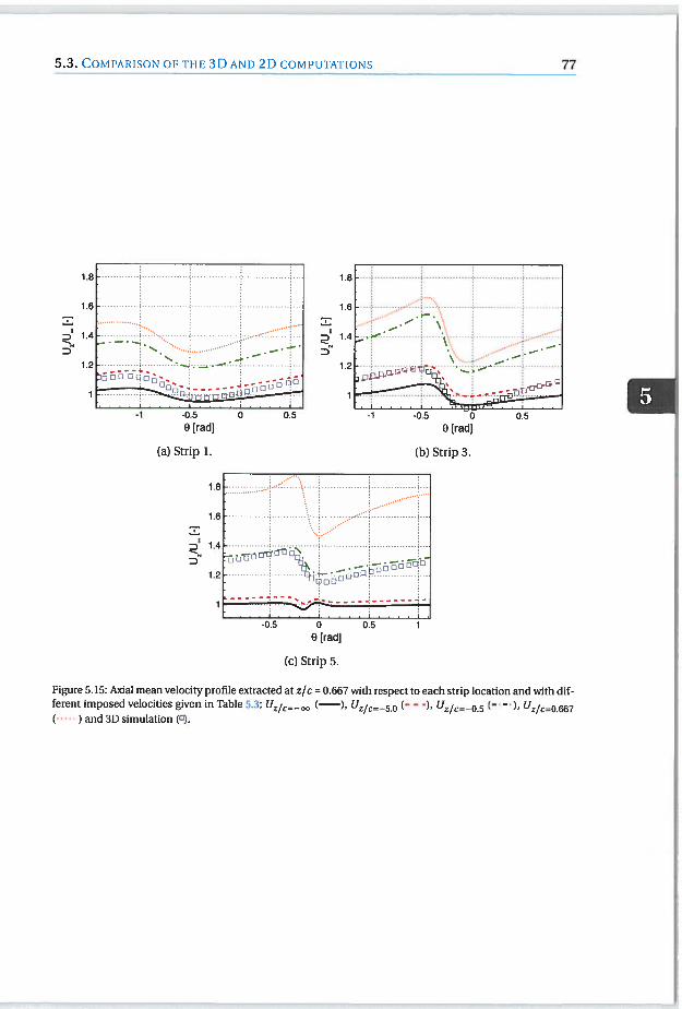
5.3. CoMiusoN OF THE 3D AND 2D COMPUTATIONS 77

i.e 1.8

1.6 1.6 -: --‘

-

.,-

D 14 I4_

D — D ——

1.2 1.2 --j-.

- DO’S s I

-1 -0.5 0 0.5 -1 -0.5 0 0.59 [rad] 0 [rad]

(a) Strip 1. (b) Strip 3.

1.8 -

1.6 .---i

D 1.4

D

1.2

1

__

0.5 - -

0 [rad]

(C) Strip 5.

Figure 5.15: Axial mean velocity profile extracted at z/c = 0.667 with respect to each strip location and with different imposed velocities given in Table 53; U2_ (—), (— — -). tJ2,i_0 ‘

and 3D simulation (U)

78 5. APPLicATiON TO DAWT

1.05

3

D0.95

0.9

-0.5

9 [rad]

(a) Strip 1.

1.05

S

D0.95

0.9

-0.5 ) 05

0 [rad]

(c) Strip 5.

Figure 5.16: Tangential mean velocity profile extracted at z/c = 0.667 with respect to each strip location andwith different imposed velocities given in Table 5.3; = —00 (—), U2j_50 ( — 1. U1_05 ( —

and 3D simulation A.

addition, it is found that these effects become less pronounced towards the outer portionof the blade. This statement can be observed for Strip 3 and Strip 5 where a better matchis obtained for the pressure distribution. Even though, the inlet velocity profile obtainedby U150 shows a better agreement with 3D simulation, it is seen that the shape of theC distribution is different for that velocity. Furthermore, at this strip location, it was already verified that the radial velocity component is weak which should have reproduceda better match. Again, it is observed that changing only the axial velocity is unable toreproduce the pressure coefficient. Contrary to the other strip locations, Strip 3 is ableto reconstruct the pressure distribution from the 2D simulation by imposing the velocityat

The mean axial velocity boundary layer profiles extracted at x/c 0.99 from the leading edge of each blade section are given in Fig. 5.19. As a general observation, the velocity profiles obtained from the 2D simulations are exposed to a higher pressure gradientcompared to the 3D case. The reason behind this, as mentioned before,might be due tothe Coriolis forces which act in the chordwise direction and have a favorable pressure ef

tho

-1 0

0 [rad]

(b) Strip 3.

1TJ.r1 S

5.3. Coipnisori OF THE 3D AND 2D COMPUTATIONS 79

0.1 4A-------------:

0.05

0 •

D-O•O5

-0.1

-0,15 •i..••j” ‘.ij.’’ ,..........,;,1’,,,,,..—.

9 Iradl

Figure 5.17; Radial mean velocity profile at z/c =0.667 with respect to each strip location; Strip 1 (A), Strip 3(.) and Strip 5 (.).

fect. For Strip 1,the velocity profiles obtained from and U10667 demonstrateseparation as also seen from the C distribution since this region has a higher pitch anglethan the other strip locations. For Strip 3 & Strip 5, a good match is observed at the outerpart of the boundary layer in comparison with the 3D simulation. In terms of the inletvelocity profile and pressure distribution, the results obtained at U1,_05 have a better agreement for Strip 5 in comparison with the 3D simulation, however, this does nothold true for the boundary layer profile. The global boundary layer variables are givenin Table 5.4 for U1_50, U1_05 and 3D simulation. Since the boundarylayer proffle obtained from U,0667 does not match with the 3D simulation, the valuesfor this case are given Appendix 13.3. From Table 5.4, it is observed that in general theboundary layer thickness, 6 and wake parameters, 11 &t /3 which are obtained from 3Dsimulations are higher than the 2D simulations while the integral boundary layer variables such as the displacement and momentum thickness values as well as the externaland friction velocity seem close to each other. However, most of the wall-pressure models are highly dependent on the wake parameters which indicates that 3D wall-pressurespectrum predictions might deviate from the 2D predictions. The boundary layer variables obtained from Uq..05 show that there is a separation for the strip location nearthe hub which can also be depicted from the boundary layer velocity profiles.

Additionally, the kinetic energy profiles are over-predicted by the 2D simulations(see Appendix B.2). The reason might be due to fact the secondary flow effects are notpresent in 2D simulation. Thus, the wall-pressure spectrum predicted by the Panton &Linebarger model will deviate significantly from the 3D predictions especially for the lowfrequencies for the suction side.

80 5. AiwiicTioN TO DAWT

Figure 5.18: Pressure coefficient along each strip location; (—) (— — -), U21_05

— ), ( ) and 3D simulation ).

5.3.3. PREDIcTIoN OF THE WALL-PRESSURE SPECTRA AND FAR-FIELD

TRAILING EDGE NOISE

The wall-pressure spectrum prediction is performed by the Kamruzzaman, Lee, andPanton &t Linebarger models for the same three strip positions that were investigatedin the previous section: a strip close to the hub Strip 1, a strip in the middle of the bladeStrip 3 and a strip near the tip region Strip 5. The wall-pressure spectrum is calculatedfrom U7=_ and Uq_5 for the Strip 1 and Strip 3 locations, while for Strip 5,is also added since it provides a better match for C and Ue (shown in Fig. 5.18 and 5.19

The dimensionless frequency for the wall-pressure spectrum is expressed by wö*/Ue

where the global boundary layer variables on the suction side are obtained from 3D simulations. Figure 5.20 shows the prediction for Strip 1 on suction side (a) and the pressureside (b). When the 3D simulation is considered on the suction side, a decay seems to occur for the prediction obtained both from the Kamruzzaman and Lee model while, thePanton & Linebarger model under-predicts for the frequencies below WS*/Ue < 10. For2D simulations, it is observed that the Kamruzzaman and Panton & Linebarger model

0

(.)

-2 uiluD

.d L

2

0

0

-2

.3

-400.8 0.20.2 0.4 0.6

xfc[-}

(a) Strip 1.

01

-2

0.80.4 0.6x/c [-]

(b) Strip 3.

0.4 0.6xIc [-]

(c) Strip 5.

5.3. Covwoisoi’t OF THE 3D AND 2D COMPUTATIONS 81

0.2 0.4 0.6 0.8

UfU5e [1

(a) Strip 1.

U/U5ei []

(b) Strip 3.

Figure 5.19: Mean axial boundary layer profile extracted at x/c =0.99 with respect to each strip location;(—), U2,_.50 (— — -), U,._05 (——1, ( ) and 3D simulation (0).

seem insensitive to the velocity increase while a significant increase is observed for theLee model above wö*/Ue > 7. On the pressure side, the predictions obtained from 3Dsimulation exhibits a similar decay, however, with different amplitudes. Likewise, thePanton & Linebarger model under-predicted the wall-pressure spectrum with respect tothe other models. When the 2D simulations are compared, it is observed that increasingvelocity shifts the amplitude for the frequencies above around wô*/Ue 2. Overall, thewall-pressure spectrum obtained by the Kamruzzaman model gives closer results with2D and 3D simulations especially for Uz/c5O.

The wall-pressure spectrum prediction for Strip 3 is given in Fig. 5.21 for the suction side (a) and pressure side (b). The predictions obtained the Kamruzzaman and Leemodels exhibit a similar decay for the high frequencies above wô*/Ue <7 for the 3D simulation on the suction side. Similarly, the Panton & Linebarger model under-predicts theamplitude for the low frequencies. The predictions obtained from the 2D simulations areinsensitive to the velocity increase even though this increase was significant for the inlet profiles and pressure coefficient as mentioned previously. The predictions obtainedfrom each model are unable to exhibit a similar curve with the 2D and 3D simulations.

C.)

>,

-0.2

I’

:

I

1.2

C.)>

U/UReI [1

(c) Strip 5.

82 5. APPLICATION TO DAWT

N

(a) Suction side. (b) Pressure side.

Figure 5.20: The wall-pressure spectrum predicted by the Kamruzzaman model (black), the Lee model (red)and the Pmton & Linebarger model (green) from (solid line), Uq,_5 (dashed line) and 3D simu

lation (rectangle) at Strip].

On the contrary, the pressure side predictions for the 3D simulations shows a similarslope, however, under-prediction occurs for the Panton & Linebarger model. The wall-pressure prediction obtained from 3D simulations of the Kamruzzaman and Lee modelsshow a better match with their predictions except for the Lee model which yields inconsistent results for higher frequencies. Overall, the Kamruzzaman model gives the mostconsistent prediction.

8C

N

Figure 5.21: The wall.pressure spectrum predicted by the Kamruzzaman model (black), the Lee model (ied),and the Panton & Linebarger model (green) from (solid line), U2,_ o (dashed line) and 3D simu

lation (rectangle) at Strip 3.

The same predictions are performed for Strip 5, in addition, the wall-pressure spectruin obtained from U1_05 is also analyzed. The wall-pressure spectrum obtainedfrom the 3D simulation with different models do not provide the same behavior for thesuction side. The wall-pressure spectrum obtained from the 2D simulations show that

(J)/U0 [-] 10e []

0

-20

(a) Suction side.

tOö/Ue l] COJ1.J I-I10’ 10”

(b) Pressure side.

5.3. Corvliusosi OF THE 3D AND 2D COMPUTATIONS 83

when the velocity increases the amplitude decreases for the higher frequencies for all themodels. For the pressure side, the Lee and Panton & Linebarger model exhibit a similarslope behavior with different amplitudes. Moreover, the frequencies above wö*/Ue> 1perform the a similar decay for all the models. In general, it is observed that increasing the velocity, decreases the amplitude for the low frequencies while increasing theamplitude for the higher frequencies except for the Panton & Linebarger model whichseems insensitive to the velocity augmentation. Similar to the other Strips, the Kamruzzaman model prediction gives similar results for 2D and 3D simulations. As a general

8C

N

0

10’ lu’

______

wö4J0 [-] to/U0 [-1

(a) Suction side. (b) Pressure side.

Figure 5.22: The wall-pressure spectrum predicted by the Kamruzzaman model (black), the Lee model (red),and the Panton & Unebarger model (green) from (solid line), U2,_5 o (dashed line), Uj_0(dashed dotted line) and 3D simulation (rectangle) at Strip 5.

remark, similar to Chapter 4, the pressure side contributes more to the higher frequencies whereas the low frequencies are dominated by the suction side. When the differentstrip positions are compared, although the Strip 5 is exposed to a higher tangential velocity, the magnitude of the spectrum seems to be closer with respect to the other striplocations. Furthermore, the low frequency range has almost the same amplitude for allthe strip locations, which means that they will contribute significantly to the far-fieldnoise spectrum. While for the high frequency range, the contribution from the last threestrips is enough to have the same amplitude. This is demonstrated in Fig. 5.23.

One-third octave band far-field noise spectrum predicted at two locations are givenin Fig. 5.24; downstream of the wind turbine (a) and upstream of the wind turbine (b).As mentioned previously, the far-field noise prediction is performed by assuming free-field propagation. In Fig. 5.24, the 2D simulations are obtained by using three differentfree-stream velocities; and Uqo5. These are compared with the3D simulation. As mentioned before, due to flow separation observed in the 2D caseof U2,_5, only the last three strips are considered for the prediction to determine ifthe high frequency range is closer to the 3D simulations as interpreted from the globalboundary layer variables. The spectrum predictions obtained by the Kamruzzaman andLee models show a difference of around 6 dB for the low frequencies which decreasesfor the middle frequencies and increases up to 2 dB for the higher frequencies, whereasthe Panton & Linebarger model under-predicts compared to the other models. This is

60

‘i;r 40

e

20

0

-20

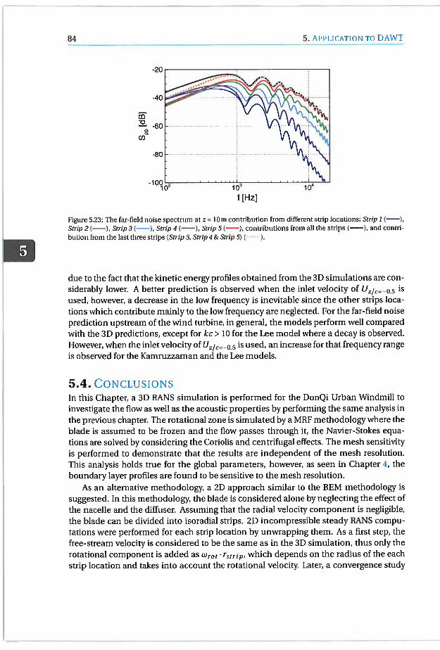
84 5. APiuci.Tloi TO DAWT

C/)

Figure 5.23: The far-field noise spectrum at z 1Gm contribution from different strip locations; Strip I (),Strip 2 (—), Strip 3 (—), Strip 4 (—), Strip 5 (—), contributions from all the strips (—), and contribution from the last three strips (Strip 3, Strip 4 & StripS) ( ).

due to the fact that the kinetic energy proffles obtained from the 3D simulations are considerably lower. A better prediction is observed when the inlet velocity of isused, however, a decrease in the low frequency is inevitable since the other strips locations which contribute mainly to the low frequency are neglected. For the far-field noiseprediction upstream of the wind turbine, in general, the models perform well comparedwith the 3D predictions, except for kc> 10 for the Lee model where a decay is observed.However, when the inlet velocity of U2,_05 is used, an increase for that frequency rangeis observed for the Kamruzzaman and the Lee models.

5.4. CoNcLusioNsIn this Chapter, a 3D RANS simulation is performed for the DonQi Urban Windmill toinvestigate the flow as well as the acoustic properties by performing the same analysis inthe previous chapter. The rotational zone is simulated by a MRF methodology where theblade is assumed to be frozen and the flow passes through it, the Navier-Stokes equations are solved by considering the Coriolis and centrifugal effects. The mesh sensitivityis performed to demonstrate that the results are independent of the mesh resolution.This analysis holds true for the global parameters, however, as seen in Chapter 4, theboundary layer profiles are found to be sensitive to the mesh resolution.

As an alternative methodology, a 2D approach similar to the BEM methodology issuggested. In this methodology, the blade is considered alone by neglecting the effect ofthe nacelle and the diffuser. Assuming that the radial velocity component is negligible,the blade can be divided into isoradial strips. 2D incompressible steady RANS computations were performed for each strip location by unwrapping them. As a first step, thefree-stream velocity is considered to be the same as in the 3D simulation, thus only therotational component is added as Wrot rst,-jp, which depends on the radius of the eachstrip location and takes into account the rotational velocity. Later, a convergence study

f[Hz]

5.4. CoNcwsioNs 85

-o

-J

(a) L at z 1Dm downstream of the wind tur- (b) Lp at z= -1Dm upstream of the wind tur

bine.

Figure 5.24: The 1/3 octave band far-field noise spectrum at two observer locations predicted by differentwall-pressure spectra predicted by the Kamruzzaman model (black), the Lee model (red), and the Panton &Linebarger model (green) from (solid line), o (dashed line), (dashed-dotted line)and 3D simulation (rectangle).

based on the number of strips is carried out by diving the blade into 5, 10, and 20 strips.It is concluded that the 5 strips configuration is sufficient for Amiet’s theory if the observer is located in the acoustical and geometrical far-field. As a second step, to takeinto account of the flow acceleration due to the nacelle and the diffuser, an axisymmetnc RANS simulation is performed without the presence of the blade. Three additionalaxial positions rather than the free-stream (z/c = —oo) are considered which are furtherupstream (z/c = —5.0), before the diffuser (z/c = —0.5) and before the blade (z/c 0.667).

The axial free-stream velocity values corresponding to these axial positions are imposedto 2D HANS simulations at each strip location.

The comparison between the 3D and 2D simulations are performed in terms of inlet velocity profiles upstream of the blade sections, pressure coefficient along the blade,and the boundary-layer proffles extracted at x/c = 0.99 normal to the blade surface atthree strip locations. It has been observed that for the axial velocity a good comparisonis achieved whereas for the azimuthal velocity, the peak point seems to be shifted whichmay indicate that the position of the blades are not identical. The radial mean velocitycomponent from the 3D simulation shows that the order of magnitude with respect tothe mean axial velocity is 10, which might have a weaker effect on the spanwise direction.The pressure distributions could not be reproduced by the 2D simulations even with different mean axial velocities at the hub region, which might be due to the centrifugal andCoriolis forces acting dominantly at that area resulting a difference between the 3D and2D nature of the flow. For the middle part, a better match is observed with respect to thehub region, however, again the magnitude of the C,, distribution seems shifted down andincreasing the velocity wouldn’t help to imitate it. On the contrary, a better match is observed for the tip region for the inlet velocity of z/c —0.5. Likewise, the C, distributionwas found to be shifted down in terms of magnitude which might create different flowfield than the 2D simulations. Finally, the boundary-layer profiles extracted at x/c = 0.99

kc [-I kc [-]

bine.

86 5. ALicivrioN TO DAWT

normal to the blade surface are investigated. In general, the boundary-layer profiles obtained form 2D simulation do not match with the 3D simulation. The last two velocities(z/c = —0.5 and z/c = 0.667) imposed to the 2D simulations demonstrate a separatedflow for the hub region. Moreover, they could not reproduce similar results compared tothe 3D simulation for the other strip locations, even though Strip 5 gives better results interms of the C, distribution. When the global boundary layer variables are considered, itis found that the boundary-layer thickness and the wake parameters have a higher valuethan the 2D simulations whereas the integral variables are found to be of the same order.

The wall-pressure spectrum is predicted by three models; the Kamruzzaman, Lee,and Panton & Linebarger iriodels for 2D and 3D simulations and the results are shownonly for three strip locations investigated before. All of the 3D predictions at differentstrip locations performed by the Panton & Linebarger model show under-predicted resuits compared to the other models. For 2D simulations, increasing the velocity fromU1_ to Uj50 does not change the predictions significantly, as it does for the inlet velocity profiles. However, further increasing the velocity, the results perform betteron the pressure side than the suction side. Overall, the Kamruzzaman model performsthe best amongst the model compared to their prediction in 3D. The far-field noise predictions are performed at 10 m upstream and downstream of the blade. The 3D prediction of Panton & Linebarger model deviates significantly from the other predictions asit is also observed for the wall-pressure spectrum. The reason for it, may be due to theunder-prediction of the turbulent kinetic energy. The 3D prediction of the other twomodels show a deviation of 6 dB maximum for the two locations. The 2D predictionsfrom the Lee and Panton & Linebarger models exhibit a good match with the 3D simulations for the low frequency part while Kamruzzaman and Panton & Linebarger modelperform better for the high frequency part. Moreover, the results obtained by the 2D simulation by imposing the velocity at z/c = —5.0 significantly improves the high frequencypart for the Kamruzzaman and Lee models, whereas it seems negligible for the Panton &Linebarger model.

In terms of computational effort, the 3D simulations are performed on a node of acluster built with AMD Opteron (tm) Processor, the computation took 1767 CPU-hour forthe finest mesh while the 2D axisymmetric and 2D strip simulation for one strip locationare performed on a work station with Intel(R) Xeon(R) CPU E5-2650 and the computation took 6.5 and 2.7 CPU-hour, respectively. In total, 2D approach for 5 strip locationswith correction for the flow acceleration inside the nacelle uses 20 CPU-hour (6.5+2.7x5)which is nearly two orders of magnitude times faster than 3D simulations.

In future work, the rotational velocity component for the 2D simulation can be variedto investigate flow field to reproduce the 3D simulations, Furthermore, the initial conditions could be obtained by a BEM method with the corrections for the 3D flow effects,and used to perform the 2D analysis.

5.4. CoNcwsioNs 87

Table 5,4: Global variables at x/c = 0.99 for different strip locations

Simulation Side Strip number ö/c Ue!UReI itr/U,ei ö*/c e/c 1-I

Strip] 0.119 1.143 0.004 0.017 0.010 3.353 6.257

Strip2 0.113 1.046 0.002 0.014 0.009 4.394 9.190

Suction Strip3 0.095 1.017 0.002 0.011 0.007 3.700 7.205

Strip4 0.081 1.005 0.001 0.009 0.006 3.109 5.611

Strip5 0.078 0.998 0.001 0.009 0.005 2.801 4.8173D

Strip] 0.038 1.092 0.008 0.004 0.002 0.440 -0.049

Strip2 0.037 0.999 0.004 0.004 0.002 0.459 -0.024

Pressure Strip 3 0.040 0.984 0.003 0.004 0.002 0.432 0.005

Strip4 0.047 0.979 0.002 0.004 0.003 0.614 0.203

Strip5 0.046 0.978 0.002 0.004 0.003 0.746 0.411

Strip] 0.045 1.040 0.004 0.015 0.007 2.0522 3.0116

Strip2 0.038 1.000 0.002 0.013 0.006 3.0698 5.5076

Suction Strip3 0.033 0.977 0.001 0.010 0.005 1.4416 1.6928

Strip4 0.028 0.959 0.001 0.008 0.004 1.0763 0.9852

Strip5 0.026 0.953 0.001 0.007 0,004 1.0192 0.881U2/c=-

Strip] 0.020 1.043 0.007 0.005 0.003 0.4695 -0.0087

Strip2 0.018 0.990 0.004 0.004 0.002 0.4983 0.032

Pressure Strip3 0.019 0.966 0.003 0.004 0.003 0.0956 -0.4412

Strip4 0.024 0.957 0.002 0.006 0.003 0.3586 -0.1569

Strip5 0.025 0.954 0.001 0.006 0.003 0.4198 -0.0768

Strip] 0.053 1.117 0.004 0.019 0.008 2.9334 5.1543

Strip2 0.046 1.037 0.002 0.018 0.007 4.6689 10.0076

Suction Strip3 0.037 0.995 0.001 0.012 0.006 1,6125 2.0461

Strip4 0.028 0.967 0.001 0.009 0.004 1.1291 1.0831

Strip5 0.026 0.956 0.001 0.007 0.004 1.0466 0.9308Uz/c=_5.o

Strip] 0.018 1.117 0.008 0.005 0.002 0.322 -0.2026

Strip2 0.016 1.025 0.004 0.004 0.002 0.3451 -0.1741

Pressure Strip3 0.018 0.983 0.003 0.004 0.002 0.116 -0.4238

Strip4 0.022 0.963 0.002 0.005 0.003 0.3453 -0.1738

Strip5 0.024 0.956 0.001 0.006 0.003 0.4182 -0.0789

Strip] - - - - - - -

Strip2 0.150 0.831 - 0.108 0.013 - -9.3629

Suction Strip3 0.056 1.061 0.001 0.023 0.009 0.3904 -0.1158

Strip4 0.037 1.003 0.001 0.012 0.006 1.3222 1.454

Strip5 0.030 0.982 0.001 0.009 0.005 1.2606 1.3337Uz/c=—o5

Strip] 0.013 1.367 0.013 0.002 0.001 0.4011 -0.1017

Strip2 0.013 1.201 0.006 0.002 0.001 - -0.6452

Pressure Strip3 0.015 1.040 0.003 0.003 0.002 0.1065 -0.4321

Strip4 0.017 0.990 0.002 0.004 0.002 0.2526 -0.285

Strip5 0.019 0.970 0.002 0.004 0.003 0.3532 -0.1638

IIEXPERIMENTAL WORK

89

F—

6A REMOTE MICROPHONE

TECHNIQUE FOR AEROACOUSTIC

MEASUREMENTS IN LARGE WIND

TUNNELS

The present study was devoted to the development and application of a remote microphone technique for aeroacoustic measurements in large aerodynamic wind tunnels.In this technique, the microphone and its connecting line to the sensing port are fittedwithin an aerodynamically streamlined fairing. A model-based calibration method wasapplied to account for the phase lag and dissipation within the microphone connectingline. The proposed system allows acoustic measurements when the wind tunnel surface cannot be altered, since the fairing can simply be glued on the wall. The fairing isstreamlined to minimize flow disturbances as well as the risk of separation which wouldotherwise contaminate the wind tunnel flow quality and acoustic measurements. It wasfurthermore hoped that the acceleration of the flow over the fairing surface might reducethe turbulence fluctuations and thereby increase the signal-to-noise ratio of the acousticmeasurements. Those aerodynamic effects were investigated with a set of hot-wire measurements performed in the subsonic L2B small wind tunnel of the von Karman Institute(VKI). The mean velocity and the turbulence intensity profile were analyzed in the presence of different inflow turbulence characteristics at 5, 10, and 15 m/s free-stream velocity. The effect of incident turbulence on the acoustic measurement was investigatedby applying the calibration procedure and comparing the measurements with a wallmounted reference microphone signal in similar flow conditions. As an application, thistechnique is used to measure the noise emitted from the contra-rotating fans of the largeLi subsonic wind tunnel of the von Karman Institute, where the microphone fairing isplaced inside the diffuser and thus subjected to a thick turbulent boundary layer.

91

6. A REMOTE MICROPHONE TECHNIQUE FOR AEROACOUSTIC MEASUREMENTS IN LARGE

92 WIND TUNNELS

6.1. INTRODUCTIONThe reduction of flow-generated noise has become one of the demanding design criteriafor numerous engineering applications. Consequently, a growth of interest has emergedin the field of experimental aeroacoustics, in order to better understand aerodynamicsound production mechanisms and to validate noise prediction methods.

Large aerodynamic wind tunnels have been and are currently being refurbished topermit measuring the noise emissions of wing components, landing gears, wind turbineblade sections, etc., at realistic Reynolds numbers Moreau et at [132J. In this context thevon Karman Institute for Fluid Dynamics (VKI) is investigating the possibility of using itslargest subsonic wind tunnel Li as a mean to study contra-rotating rotor (CRR) noise. Inthis instance, the CRR under consideration is the twin-rotor fan that provides the flow tothe wind tunnel. In order to measure the tonal and broadband noise resulting from theviscous wake interactions, an array of wall-mounted microphones has been designed, tobe located in the divergent section of the wind tunnel (Fig. 6.1).

The following guidelines drove the design:

1. The number and spatial distribution of microphones should permit extracting theacoustic field in terms of its duct modal components, up to the second azimuthalmode.

2. The placement of the microphones should not require drilling into the thick

(about 0.3 m) concrete walls of the divergent section. As a result, the microphonesshouid be encapsulated within fairings, to be glued on the inner wall of the divergent section.

3. The microphones fairings should not introduce additional turbulence, for the sakeof flow quality in the test section firstly, and secondly to avoid extraneous noisegeneration by the guide vanes at the downstream end of the divergent section.

4. If possible, the fairings should enhance the signal-to-noise ratio between the incident acoustic field and the hydrodynamic pressure fluctuations induced by theturbulent boundary layer (TBL) at the microphone locations.

Figure 6.1: The Li wind tunnel.

6.2. MIcu0PH0NE FAIRING 93

While the first aspect above won’t be treated in this paper — it is discussed in length inthe literature, e.g. by Sack et al. [160], the other objectives and proposed solutions aredetailed in what follows.

The structure of the chapter is the following: Section 6.2 describes the technical solution adopted to meet the above objectives, which implies a modelling of the acousticresponse of the system (Section 6.3) and evaluating the influence of TBL pressure fluctuations on the measurement accuracy (Section 6.1). Conclusions are drawn in Section 6.5.

6.2. MIcRoPHoNE FAIRINGIn order to minimize flow separation, which would otherwise alter the wind tunnel flowquality and contaminate the microphone signal, the fairing encapsulating the microphone was designed using a streamlined profile, shown in Fig. 6.2(a). It is a combinationof two arcs in which the trailing edge radius, 0.2 m, is twice the leading edge radius. Thefairing has 0.224 m length, maximum height of 0.047 m and maximum width of 0.12 m.This shape is not the result of an aerodynamic optimization, but follows empirical guidelines to mitigate the risk of flow separation with a size compatible with the curvature ofthe wind tunnel wall. The microphone is lying horizontal to minimize blockage, and itsholding part was designed in a modular way, such that it can be disassembled from thefairing and fitted on a calibrator shown in Fig. 6.2(b). The aim here is to permit a calibration as close to in-situ conditions as possible, accounting for the acoustic response ofthe channel and cavity that lead from the pressure port to the microphone membrane.The dimensioning of the line-cavity system was performed by means of a linear responsemodel detailed in Section 6.3, together with its experimental validation.

(a)

Figure 6.2: CAD drawing of (a) the fairing, the holding part with the microphone and the assembly, (b) thecalibrator with the holding parts and a reference microphone.

Another purpose of the design, justifying the position of the pressure tap on the fairing top, is to take advantage of the local acceleration that occurs from the leading edgeof the fairing. This is an attempt to reduce the turbulent fluctuations and improve the

(b)

6. A REMOTE MICROPHONE TECHNIQUE FOR AEROACOUSTIC MEASUREMENTS IN LARGE

94 WIND TUNNELS

relative importance of the acoustic signal. Section 6.4 details the hot wire measurementsthat were conducted over the fairing in order to quantify the effect of the acceleration onthe turbulence intensity, and to correlate this effect to the quality of the acoustic measurements.

6.3. LINE-cAvITY RESPONSE MODEL

The microphone is connected to the pressure port via an L-shaped line and cone shapedcavity system as shown in Fig. 6.3(a). The length and diameter of the line, as well asthe cavity volume, have an important effect on the amplitude and phase lag of the pressure fluctuations sensed by the microphone membrane. Since the frequency responseof the line-cavity system can exhibit strong resonances that are detrimental to the measurement accuracy, several methods can be employed to damp out the resonance. Apossibility is to use a small diameter flexible tube. However, this can introduce a signaldistortion. Another method is to insert dampers to suppress the resonance in the systemas described in Surry and Stathopoulos [1791. Eventually, the most promising solutionwas found to consist in correcting the signal based on the measured transfer functionof the system. A correction of the amplitude is sufficient when single sensor measurements are to be processed, but in our case a phase calibration is also needed since theduct modal eduction makes use of the phase between different microphones. An example of a digital correction technique using the inverse transfer function was introducedby Irwin et al. [1051. This strategy will be followed in this paper, using the measuredtransfer function 114, 1471.

TotalDiameter (2R) Volume

oithePipe

(b)

Figure 6.3: (a) Microphone holding part, inserted in the fairing as shown in Fig. (S.2(a); (b) its simplification asa line-cavity system.

The analytical models that simulate the dynamic response of the tube are investigated by Bergh and Tijdeman [21] and citetstinson amongst others [10, 84, 196]. Thesemodels account for compressibility effects, viscous dissipation, heat loss, and elastic expansion [100]. In this paper, the remote microphone technique will be compared withthe Bergh and Tijdeman [21] model. The model is expressed as a linear time-invariantsystem subjected to small amplitude perturbations.

(a)

6.3. LINE-cAvITY RESPONSE MODEL 95

The transfer function between the pressure at the port opening and the pressuresensed by the pressure sensor is given by Bergh and Tijdeman [211:

r vt 1\ i’Lc0sh2(I’) + — a

+ —) ncbLsinh(cPL)j (6.1)P0 Vt k

where=

with a i3!2Rv/ is the shear wave number where the viscosity is taken into account, i is the imaginary unit, R is the tube radius, Ps j5 the mean

density, v is the frequency, i is the absolute fluid viscosity, ii [i +

is a polytropic constant, Pr is the Prandtl number, y = Cr/C,, is the specific heatratio, J7, is the Bessel function of first kind of order in, a0 is the mean velocity of thesound, L is the length of the pipe, V and V are the pressure transducer and tube volume, a is the dimensionless increase in transducer volume due to diaphragm deflection,and k is the polytropic constant for the volumes [211. This model was implemented in aVKI in-house MATLAB code named PreMeSys [331.

The three geometrical parameters which affect the frequency response function arethe line radius, length, and the cavity volume. Their influence has been quantitativelyvalidated using the results of Bergh and Tijdeman [211. Since the amplitude and frequency of the resonance are most sensitive to the line radius and the line length, thesevariables represent the most effective design parameters. In contrast, changing the cavity volume within the limits of practicality does not affect significantly the resonancefrequency. A high resonance frequency of the system would be achieved with small linelength and cavity volume, and a large line radius. However, a large diameter increasesthe probing area, leading to a degradation of the spatial resolution and aliowing turbulence to contaminate the microphone measurements.

Their influence is investigated in Fig. 6.4. The results permit validating the PreMeSyscode. They also indicate that

• increasing the line radius has the effect of increasing the resonance frequency, aswell as its amplitude as a result of lower viscous losses;

• increasing the line length increases the propagation time and adds viscous losses,such that both resonance amplitude and frequency decrease;

• increasing the volume adds a buffer for the acoustic propagation in the system,leading as well to a reduction of the resonance amplitude and frequency.

6.3.1. DESIGN OF THE FAIRINGSThe pipe length and radius, as well as the cavity volume, were designed to avoid a potential flow and acoustic coupling as observed byTonon et al. [1881. In such a feedbackmechanism, the vortex shedding at the port aperture couples with the acoustic responseof the branch at the closed end. The vortex shedding at the port aperture was characterized by a Strouhal number St = 2fR/Uo observed around 0.4, where U0 is the velocityabove the aperture. A small pipe radius R is desirable for the sake of spatial resolution,

96

6. A REMOTE MICROPHONE TECHNIQUE FOR AEROACOUSTIC MEASUREMENTS IN LARGE

C.,cc

1.50

ccC.)

0

0 50 100 150 200 250 300Frequency (Hz)

(c)

WIND TUNNELS

Figure 6.4: Validation of PreMeSys by comparison with results of Bergh and Tijdemai 1211 and effect of geometrical parameters. (a) effect of pipe radius (L = 0.5m V = 300 i0 m3); (b) effect of pipe length(R= 0.75 i0 in, V = 300• 10 m3); (c) effect of cavity volume (L= 1 m, R = 0.75. i0 m). a = 0 and k= 1.4.

6

00cc

0

cc0

E

! —R=O.50-10’m—

- ROJ51O’m—

— R=l.2510’m0 Bergh & Tijdeman

I •

,dd b

,, S

00ccC0

cc0

0.6

0 50 100 150 200Frequency (Hz)

(a)

‘—C 300250 300 ) 50 100 150 200 250Frequency (Hz)

(b)

erna

6.3. LINE-cAvITY RESPONSE MODEL 97

with the smallest radius that can be drilled with precision being 0.5 i0 m. Three pipe-cavity systems with a radius size of 0.5- i0, 1.0. i0, and 1.5 i0 m were calculatedwith PreMeSys to obtain the acoustic resonance frequency. The equivalent line-cavitymodel is illustrated in Fig. 6.3(b), where the total volume of the equivalent cavity includes the volume between the protection grid and the membrane. The geometricalparameters were calculated from the CAD model as indicated in Table 6.1. The resultsobtained with PreMeSys are shown in Fig. 6.5.

Radius- 10 (m) Length 10 (ml Volume- 10 (md)

0.5 30.4 3041.0 30.9 3041.5 31.4 299

Table 6.1: Parameters for the pipe-cavity systems of Fig. 6.3.

For the targeted application presented in Section 6.4.3, the grazing flow velocity Uois of the order of 10 m/s. The frequencies corresponding to St = 0.4 are fst = 4kHz, 2 kHzand 1.3 kHz for radii of 0.5 i0 m, 1.010 m, and 1.5 i0 m, respectively. From Fig. 6.5,it can be observed that the acoustic resonance frequencies of the pipe-cavity systems forR 0.5- i0 m and 1.0 i0 m are well below those values, which should thus not leadto spurious flow-acoustic resonances. A pipe radius of 1 mm was finally selected as itprovides a nearly constant gain for the frequency range of interest for the applicationdescribed in Section 6.4.3, which is [0,500] Hz.

0C.)

UC0.10C.)

aE<0

0 1000 2000 3000Frequency (Hz)

Figure 6.5: Investigation of the parameters in Table 6.1 with PreMeSs.

6.3.2. CALIBRATIoN PRocEDuREThe static calibration was performed by using the B&K Sound Calibrator Type 4231. Thecalibrator emits a continuous signal at 1 kHz with a sound pressure level of 94 dB. The dynamic calibration was performed with the calibrator shown in Fig. 6.2(b). A loudspeakerwas placed on one side of the calibration tube and, on the other side, the microphoneswere distributed equally at the same axial position.

The data acquisition was performed by National Instrument cDAQ-9178 with twomodules: NI 9215 for the microphones and NI 9263 for the loudspeaker. B&K 4938A-

4000

6. A REMOTE MICROPHONE TECHNIQUE FOR AEROACOUSTIC MEASUREMENTS IN LARGE

98 WIND TUNNELS

011-1/4-inch pressure-field microphones with Type 2670 preamplifier were connectedto the B&K Nexus conditioning amplifier Type 2960-A. The microphones were exposedto a chirp signal, where the frequency range starts from the lowest frequency emittedfrom the loudspeaker (fj, 100 Hz) up to the cut-off frequency of the pipe (finax 5kHz). The sampling rate was chosen as 51.2 kHz with 220 samples. A reference microphone was flush-mounted to determine the response of the pipe-cavity system for thethree different configurations. The measured transfer function is defined as [30, 961:

H(f) (6.2)

where 1 denotes the reference microphone and 2 is the pipe-cavity system, S21 is thecross power spectral density of the reference microphone and the pipe-cavity systemand S1, is the power spectral density of the reference microphone. The transfer functionis calculated by tfestimate MATLAB code, which uses Welch’s averaged, modified penodogram method. The signals are divided by 216 segments with 50% overlap by applyingHanning window. Afterward, the periodogram of each segment is calculated and thespectral densities are averaged.

The pipe-cavity system was machined out of a block of Teflon. Three designs withthree different pipe radii have been tested using the calibrator to obtain the transfer function. The results are shown in Fig. 6.6 for the largest of the three radii, R1.5 x i0 m, and for 8 different realizations of the same design. The results indicatethat both for the magnitude and phase, significant discrepancies are observed betweenthe measured transfer function and the theoretical model, and even between differentrealizations, in spite of similar manufacturing qualities. In terms of amplitude, the measured values are significantly below the prediction, which we conjecture can be due tothe mechanical compliance and roughness of the material. This was also observed byHurst and Van De Weert 11001, who also used Teflon.

6.4. AERODYNAMIC EFFECTS OF THE FAIRING ON THE ACOUS

TIC MEASUREMENTS

Hot-wire measurements and acoustic measurements have been performed with andwithout the fairing in the L2B wind tunnel of VKI to assess the effect that the fairinghas on the grazing flow at the sensing port. L2B is an open circuit wind tunnel of suctiontype with a 4.4 kW variable-speed DC motor providing a maximum velocity of 35 rn/s.The rectangular test section, shown in Fig. 6.7, is H = 0.35 m high, 0.35 m wide, and 2 IT1

long. The fairing, with maximum height at the sensing port equal to 0.13H, was placedat a distance 3.86H downstream of the inlet. The boundary layer measurements wereobtained at a single axial position above the sensing port of the pipe-cavity system. Areference microphone was placed at the same axial and spanwise location, but flush-mounted on the opposite wall. A Prandtl tube was used to measure the free-stream velocity at channel mid-height. The hot-wire and acoustic measurements were performedwith a sampling frequency of 51.2 kHz with 220 samples.

6.4. AERoDYNAMIc EFFECTS OF THE FAIRING ON THE ACOUSTIC MEASUREMENTS 99

15C.)Ce- 10-0

Ceci 5-0E

50

____________________

—Calibrated Signal[r -Bergh &Tijdeman Model]

0 1000 2000 3000 4000Frequency (Hz)

(b)

Figure 6.6: Comparison of the experimental calibration with the PreMeSys prediction. (a) amplitude of thedynamic response; (hi phase of the dynamic response.

00

I—Calibrated SignalL— —Bergh & Tijdeman Model

1000 2000 3000 4000Frequency (Hz)

(a)

0)0

0)-50

-100C,)

-200

Turbulence GeneratingBlocks (TG8)

Figure 6.7: L2B wind tunnel setup.

6.4.1. AERoDYNAMIcs

The mean velocity profile and the turbulence intensity are shown in Fig. 6.8, for threedifferent velocities: 5, 10, and 15 mIs. Here, y is the distance from the surface of thewind tunnel lower wall, or from the surface of the fairing when the latter is in place. Urefis the reference velocity measured at channel mid-height, used for the calculation of the

turbulence intensity Ti. !Uref. In the presence of the fairing and for a canonicalflat plate incoming turbulent boundary layer, Fig. 6.8 (up) shows that the velocity accelerates and causes a reduction of the turbulence intensity over most of the boundary

6. A REMOTE MICROPHONE TECHNIQUE FOR AEROACOUSTIC MEASUREMENTS IN LARGE

100 WIND TUNNELS

layer height, except close to the surface where the turbulence intensity remains mostlyunaffected.

A second measurement campaign was conducted, to evaluate the effect of the fairing subjected this time to a highly turbulent boundary layer, produced by turbulence-generating blocks (TGBs). Rectangular cross-section blocks extending over the full channel span perpendicuiarly to the mean flow, with streamwise dimension 0.057 H andheight 0.086 H, were placed at 2.14 H upstream of the fairing leading edge (see Fig. 6.7),on the bottom and upper walls of the wind tunnel. A longitudinal separation betweenthe TGB and the microphones around 25 block heights ensures that the microphonesare well beyond the reattachment of the block-induced separation bubble, even if theredeveloping turbulent boundary layer has probably not reached equilibrium yet whenreaching the microphones. This is not considered an issue, the purpose of this study being mostly to obtain a thicker and more turbulent boundary layer at the location of thesensing port.

The same reference velocity as before, Uref = 5,10 and 15m/s, was maintained atchannel mid-height. The mean velocity and turbulence intensity profiles, obtained withthe TGBs in place, are shown in Fig. 6.8 (bottom). The boundary layer thickness appearsto be substantially larger than in the clean case, as desired. In this high turbulence case,while the acceleration of the mean flow induced by the fairing is still significant, thebenefits in terms of turbulence reduction are mitigated: reduction is only observed fory/H>0.06 while a substantial increase of the turbulence is found closer to the sensingport, with turbulence levels in excess of 20% to be compared with the 13-14% that wasmeasured in absence of fairing. This is anticipated to be detrimental for the acousticmeasurement accuracy.

6.4.2. AcousTic MEASUREMENTS

Two measurement campaigns were conducted. In the first one, a lousdpeaker is used,and fed with a low-frequency signal in order to generate a plane wave at the axial locationof the L2B duct where two microphones are located (see Fig. 6.7). In the second one, noloudspeaker is used and the background noise of the L2B wind tunnel is measured.

First acoustic measurement campaign: using a loudspeaker source

The acoustic pressure spectra below are expressed as Sound Pressure Levels (SPL) usingthe conventional reference pressure of 20 pPa. The power spectra were computed bypiveich MATLAB code and the required parameters were chosen to be the same as inthe calibration procedure. For the first acoustic measurement campaign, a chirp signalspanning from 10Hz to 500 Hz was used, the first transversal cut-off frequency of theduct corresponding to kH = ir being 485 Hz [951. The reference microphone being flush-mounted, it is directly exposed to the incident acoustic field and incoming turbulentpressure fluctuations. The second microphone is installed in the aerodynamic fairing,with its sensing port at the same axial location, and should therefore sample the sameacoustic signal in both amplitude and phase. From the results of Section 6.4.1, one mighthowever expect different pressure measurements owing to the different evolutions ofthe boundary layers sensed by the reference and fairing microphone. It was therefore

6.4. AERODYNAMIC EFFECTS OF THE FAIRING ON TI-IE ACOUSTIC MEASUREMENTS 101

. if— W:thoUt fuihng 5m/s /— —

— With tairing 5m/s / i Iwithout tairing 1cm/s / I I

— —— with tairirg 1 0w/s /

Without taiting ibm/s / IWith fairicg ibm/s

0_

— without airing 5m/s— —

— with fairing 5mb— without taring 10w/s— —

— with fairing 10w/swithout laiting 15w/swith faiting 15w/s

z>..

0

— without ta/aug 5w/s— — — with fairiog bmis— without faiting tOm/s— —

— with fairiog t 0w/swithout fairing 15m/swith fairfng 15w/s

10 15 20T.l.%

0.25

0.2

‘ 0.15>

0.1

0.05

0.25

0.2

0.15>

0.1

0.05

0.5 1 “0 5u/u ref

(a) (b)

>.

10u/u ref

(C) (d)

Figure 6.8: Mean velocity profiles (left) and turbulence intensity profiles (right), with a clean incoming boundary layer (up) and in presence of upstream turbulence-generating blocks (down), for free-stream velocitiesUref = 5,10 and 15 m/s.

6. A REMOTE MICROPHONE TECHNIQUE FOR AEROACOUSTIC MEASUREMENTS IN LARGE

102 WIND TUNNELS

verified a priori that the amplitude of the loudspeaker excitation is sufficiently abovethe background noise of the L2B facility. The results shown in Fig. 6.9 indicate that thiscondition is fulfilled at 10 m/s, for which the loudspeaker level is at least 10 dB above thebackground noise of the facility. This is true except for frequencies below 60 Hz, wherethe wind tunnel longitudinal resonances dominate, and at the Blade Passing Frequencyof the axial fan (121 Hz and 176 Hz for 10 rn/s and 15m/s, respectively) and its higherharmonics. For U 15 m/s, the background noise cannot be considered as negligibleover a large range of frequencies. Thus, the following results focus on the 10 rn/s caseaccordingly.

100 fl’-—-r—

.

50 E [ckground Noise lOm/s—LSon 10 rn/s

Background Noise 15m/sLSonl5m/s

0•100 200 300 400 500

Frequency [Hz]

Figure 6.9: Amplitude of the loudspeaker excitation compared with the L2B background noise for U = 10 m/sand 15m/s,

The transfer function obtained from the calibration procedure is applied in theFourier domain to the signal received from the fairing to calibrate the signal:

M(f)R(f)

H(f)(6.3)

where M is the raw signal received from the fairing, H is the transfer function given inEq. (6.2) and R is the calibrated signal. Fig. 6.10 permits comparing the wall pressure signal, the raw signal and the calibrated signal at 10 m/s. The effect of the correction is relatively minor over most of the frequency range (consistently with Fig. 6.6), but reaches anon-negligible difference of 5 dB at 460 Hz, where it still permits an acceptable compensation. Above 460 Hz (kH = 2.98), the appearance of slowly decaying cut-off transversemodes can probably explain the discrepancy between the acoustic fields measured atthe upper and lower plates, the loudspeaker being mounted on the upper ‘vall at only2H of longitudinal distance upstream of the microphones section.

With regard to the phase compensation, Fig. 6.11 shows the phase between the wallpressure signal and fairing microphones (theoretically zero for the plane wave mode),without and with compensation applied to the latter. Consistently with the phase calibration shown in Fig. 6.6, it can be seen that the phase compensation is relatively minorin this frequency range, but still brings an improvement with respect to the raw signal.

Second acoustic measurement campaign: measuringfiwility background noise

6.4. AERoDYNAMIc EFFECTS OF THE FAIRING ON THE ACOUSTIC MEASUREMENTS 103

100 —

‘ 80

60 - —Wall Pressure Signal— Raw Signal

Calibrated Signal40

100 200 300 400 500Frequency [Hz]

Figure 6.10: Comparison of the wall pressure signal, the raw signal, and calibrated signal, U,,, = 10 m/s.

150—Signal

1oo

Calib,,,A

100 200 300 400 500Frequency [Hz]

Figure 6.11: Phase difference berween the wall pressure signal and fairing microphones, without and withphase compensation for the latter.

6. A REMOTE MICROPHONE TECHNIQUE FOR AEROACOUSTIC MEASUREMENTS IN LARGE

104 WIND TUNNELS

The objective of the second acoustic measurement campaign is twofold: i) to assess theeffect of the compensation for a wider frequency range including the resonance of thepipe-cavity system (observed to lie around 700 Hz in Fig. 6.6), and ii) to quantify the impact of the aiteration of the turbulent flow by the fairing, observed in Section 6.4.1, on themeasured pressure fluctuation. For those measurements, the loudspeaker is not used,and the background noise produced by the L2B facility serves as test signal.

The considered frequency range extends up to 5kHz. Note that the pressure spectra shown below, including non-negligible turbulent pressure components for some frequencies, are still expressed in terms of Sound Pressure Levels with a reference pressureof 20 !lPa. It was verified as a preliminary step that the extended pressure spectra aresimilar on both lower and upper walls of the test section when measured with flush-mounted microphones. Figure 6.12 confirms this assumption, permitting in what follows the comparison of flush-mounted microphone measurements at the upper wallwith fairing microphone measurements at the lower wall under identical flow conditions. Similar conclusions were reached for a free-stream velocity of 15 m/s, and also inpresence of the turbulence-generating blocks.

100 I

80

60 .,,.,

& , IIi.(.1) -

‘+0 —Upper, ‘.

Lower20

101 102

Frequency [Hz]

Figure 6.12: \VaIl pressure spectra measured at the upper and lower walls of the L2B test section using flush-mounted microphones.

The case without TGB is discussed first. The effectiveness of compensating the fairing microphone measurements using the measured calibration function is quite obviousin Fig. 6.13, especially in the range [600-9001 Hz where it removes the resonance of thepipe-cavity system, and above 1 kHz where it corrects for the attenuation in the line.Concerning the alteration of turbulence due to the fairing, comparing the calibratedsignal and flush-mounted microphones measurements does not allow to discern anysubstantial difference in spite of the strong acceleration of the flow and substantial reduction of the turbulence intensity (at least far enough from the wall) that were observedin Fig. 6.8 (top). This can be an indication that the measured pressure fluctuations aremostly radiated by the facility and of acoustic nature, and/or that the local wall pressurefluctuations are mostly induced by the near-wall turbulence, which was indeed observedto not vary significantly in Fig. 6.8 (top-right).

Since comparing the spectra at lOm/s and 15m/s doesn’t allow to elucidate theacoustic vs. turbulent nature of the measured pressure fluctuations, the attention is nowturned to the measurements performed with the TGBs, forcing larger incoming turbu

100

Pressure Signal

Calibrated Signal

Frequency [Hz](b)

6.4. AERoDYNAMIC EFFECTS OF THE FAIRING ON THE ACOUSTIC MEASUREME\TS 105

-o-J

C’)

50

0101 102

Frequency [Hz](a)

100

-o500(I)

0

PF—Wall Pressure Signal—Raw Signal

Calibrated Signal

101 102 1o3

Figure 6.13: Effect of the fairing microphone compensation on the measured pressure spectrum for (Jco =

lOm/s (a) and 15m/s (b). Clean incoming boundary layer.

6. A REMOTE MICROPHONE TECHNIQUE FOR AEROACOUSTIC MEASUREMENTS IN LARGE

106 WIND TUNNELS

lence intensities. The effect of the TGB is quantified by the flush microphone spectra

shown in Fig. 6.14, where the frequency axis has been rescaled by the Blade Passing Frequency (BPF) to facilitate comparison, since the fan speed had to be slightly adjusted tomaintain the free-stream velocity in presence of the TGBs. The effect of the increasedturbulence is mostly visible below the first BPF where the levels are increased by about5 to 10dB depending on the flow speed, compared with the clean TBL case. At higher

frequencies the spectrum seems to be dominated by the background acoustic noise of

the facility, both in terms of tonal and broadband content.

100

50

1

0

thtTGB Ji10-2 100 102

Frequency/BPF(a)

100

—without TGBwith TGB

Qi

102 10° 102

Frequency/BPF(b)

Figure 6.14: Effect of the turbulence-generating blocks on the spectra measured by the flush-mounted micro

phone for U tOm/s (a) and 15m/s (b).

In contrast, the acoustic spectra measured by the fairing microphone (Fig. 6.15) exhibit shape and levels that indicate a more intense contribution of the turbulent pressure fluctuations for the fairing microphone than for the flush-mounted one. The in

creased turbulence pressure levels range from 3-5 dB at low frequencies below the BPF, to

reach about 10 dB above 1 kHz at 15 mIs. This result is consistent with the substantial in

crease of the turbulence intensity close to the fairing surface that was reported in Fig. 6.8(bottom-right) from the hot wire measurements. This investigation doesn’t permit to re

solve whether the increase of the measured turbulence pressure levels is predominantlycaused by the flow acceleration over the fairing, or due to the sensing location being de

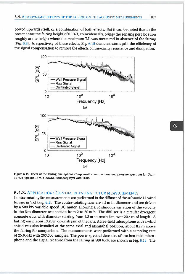
6.4. AERoDyNAvIIc EFFECTS OF THE FAIRING ON THE ACOUSTIC MEASUREMF<TS 107

00r

50

—Wall Pressure Signal—Raw Signal—Calibrated Signal

101 102

Frequency [Hz](b)

Figure 6.15: Effect of the fairing microphone compensation on the measured pressure spectrum for U =

lOm/s (up) and 15 m/s (down). Boundary layer with TGB5.

6.4.3. APPLICATIoN: CONTRA-ROTATING ROTOR MEASUREMENTSContra-rotating fan measurements are performed in the diffuser of the subsonic Li windtunnel in VKI (Fig. 6.1). The contra-rotating fans are 4.2 m in diameter and are drivenby a 580 kW variable speed DC motor, allowing a continuous variation of the velocityin the 3m diameter test section frotn 2 to 60 mIs. The diffuser is a circular divergentconcrete duct with diameter starting from 4.2 m to reach 6 m over 20.4 m of length. Afairing was placed 13.20 m downstream of the fans. A free-field microphone with a windshield was also installed at the same axial and azimuthal position, about 0.1 m abovethe fairing for comparison. The measurements were performed with a sampling rateof 25.6 kHz with 200,000 samples. The power spectral densities of the free-field microphone and the signal received from the fairing at 500 RPM are shown in Fig. 6.16. The

ported upwards itself, or a combination of both effects. But it can be noted that in thepresent case the fairing height of 0.13H, coincidentally, brings the sensing port locationroughly at the height x•vhere the maximum T.I. was measured in absence of the fairing(Fig. 6.8). Irrespectively of these effects, Fig. 6.15 demonstrates again the efficiency ofthe signal compensation to remove the effects of line-cavity resonance and dissipation.

100

50

0

—Wall Pressure SignalH—-Raw Signal

Calibrated Signal

101

-o-Ja-C/)

0

-Ja-Cl)

102 i03Frequency [Hz]

(a)

0

6. A REMOTE MICROPHONE TECHNIQUE FOR AEROACOUSTIC MEASUREMENTS IN LARGE

108

-.

WIND TUNNELS

12C —.—..— -

100

- Raw Signal°- 60 —Calibrated Signal

Free—field Signal

_____________

102 - 1Frequency [Hz]

Figure 6.16: Comparison of the free-field microphone, raw and calibrated signals, 500 RPM.

signal received from the fairing is calibrated by applying the transfer function obtainedfrom the calibration procedure described above. In the raw signal, a strong resonancepeak around 0.75 kHz followed by an anti-resonance are observed due to the pipe-cavitysystem. However, after calibrating the signal using the measured transfer function, theartifacts of the line-cavity oscillating response are eliminated and a good match with thefree-field wind-shielded microphone is obtained.

6.5. CONCLUSIONS AND PERSPECTIVES

The present work describes an experimental technique aimed at measuring aerodynamic noise in closed test section wind tunnels. The fairing approach permits installingmicrophones in wind tunnels where the duct walls cannot be conveniently altered, whileminimizing the flow disturbances. The microphone is positioned horizontally inside thefairing and is remotely connected to the test section through a pipe-cavity system.

The design of the pipe-cavity system was performed following an analytical model,which proved good enough to derive the main dimensions. The model did however exhibit too much deviation from the measured response function to be used for calibration. A systematic calibration procedure has to be applied to each individual microphone line-cavity holder, which permitted to accurately compensate for the resonanceand attenuation of the system.

The aerodynamic effect of the fairing was investigated in a small wind tunnel bymeans of hot-wire measurements for different velocities, and for low and high turbulence intensities. While it was verified that the fairing induces a strong acceleration ofthe flow, the expected benefits in terms of turbulence reduction were not observed. Forthe clean wall turbulent boundary layer case, the reduction of turbulence only occursfar from the wall but remains mostly unaffected in the immediate vicinity of the surface.And in the high incoming turbulence case, the near-wall turbulence is even observed toincrease significantly in the presence of the fairing.

As a practical application, the noise emitted by the contra-rotating fan of the subsonic Li wind tunnel was measured. A fairing was installed in the downstream part ofthe diffuser, together with a free-field microphone protected by a windshield. The positive match between the compensated fairing and free-field signals demonstrate again

6.5. CoNcLusioNs AND PERSPECTJ\1LS 109

the effective compensation of the line-cavity resonance and attenuation effects. Thisvalidates the concept of fitting the microphones in an aerodynamically-shaped fairingto avoid introducing flow disturbances. However, further research is needed to reacha more thorough comprehension of the acoustic vs. hydrodynamic content of the measured signals. This might be achieved through modal decomposition of the pressure fieldmeasured by multiple fairing microphones, in order to extract the pressure componentmatching the expected acoustic propagation pattern in a slowly-diverging duct.

ci

7AN INVESTIGATION ON THE EFFECT

OF THE INFLOW QUALITY

This section focuses on a preliminary experimental campaign to investigate the effectof inflow conditions on the aerodynamic performance and aeroacoustic installation effect for a Building Integrated Wind Turbine (BIWI). The building model of Brussels Finance Tower from a former study [141] is used with the straight duct model and wind turbine model. Two types of neutral Atmospheric Boundary Layer (ABL) conditions, fromslightly rough and moderately rough classes, generated in the VKI L-1B wind tunnel areused for investigation of turbulence effects, and six angles from 00 to 75° are used to investigate the inflow orientation. The power measurements are performed for a wind turbine within the building and another one placed on the top of the building with varyingangle of attacks and different inflow conditions. Furthermore, acoustic measurementswithin the duct are performed by nine flushed-mounted microphones with varying inflow characteristics and direction.

7.1. INTRODUCTION

Wind turbines have been utilized mainly in rural areas due to available space and established wind resources. As a drawback, it has sometimes caused a significant alterationof the landscape. Also, losses incurred during the transportation of electricity to the residential areas are penalizing the global efficiency. For these reasons, integrating windturbines into the building environment is currently being considered, as it should minimize those loses and cause less damage to rural areas. However, there are some disadvantages as it is unsuitable to construct wind farms not only due to the lower speed andhigh turbulence caused by the surface roughness of the complex building arrangementbut also due to the lack of space for large wind turbines in urban areas 11451. For this aspect, high-rise buildings offer an interesting compromise as the surface roughness hasless effect on the urban area at higher altitudes, thus resulting in a higher velocity andlow turbulence. Also, with a correct arrangement of the buildings, a funnel effect could

111

112 7. AN INVESTIGATION ON THE EFFECT OF THE INFLOW QUALITY

Figure 7.1: BLWT system using wind turbines: (a) three possible installations for large-size wind turbines, and(b) two possible installations for small size wind turbines [1451.

be created [145]. Both of the aspects would lead to a velocity augmentation and thus, ahigher power output. These types of wind turbines which are integrated to a building arecalled Building Integrated Wind Turbines (BIWT). Depending on the size of the wind turbine, the installation locations might change as illustrated in Fig. 7.1. For the small windturbines, there are two possible installation locations: on top or alongside the building.For the wind turbines larger in size, they can only be placed on top or alongside thebuilding, or within a duct.

Utilizing the small wind turbines within the building is considered an economicalmethod, since the existing building can be used without additional modifications andstructural strengthening [145]. However, the total output is found to be lower than thelarger wind turbines since they can be installed into limited spaces [145]. For the largerwind turbines, the main issue is the structural strengthening due to the wind loads exposed to the wind turbine. Therefore, additional precautions need to be taken.

Regarding the installation location strategy of wind turbines, the configuration ontop of buildings benefits from the higher wind speed as well as the less turbulentflow [177]. Moreover, the wind turbine location on the rooftop is interesting to avoid therecirculation zone of low velocity and high turbulence which is caused by the edge of thebuilding. However, with wind turbines within an adjacent building or in a duct through abuilding, there is a benefit in the pressure difference between upstream and downstreamfaces of the building, which induces the velocity through the channel. The investigation conducted by BDSP Partnership [177], comparing seven BIWT configurations with

a)

b)

7.2. EXPERIMENTAL SETUP, ACQUISITION CHAIN, AND POST-PROCESSING 113

their base model at the same height, found that the circular duct with smooth edges produces the maximum power production with respect to the different wind types of uniform wind, wealdy and strongly unidirectional wind, and hi-directional wind. Althoughthis configuration produces the maximum power generation, this also contributes to theacoustic nuisance due to the horn effect of such installation, which is particularly problematic in a densely populated urban environment. Moreover, the sound generationprocess is quite sensitive to the quality of the inflow, which can vary sensibly depending on the integration of the setup in the building, on the wind speed and direction, etc.Research is thus needed to better understand the aerodynamic performance vs. noisetradeoffs that can be achieved by BIWT configurations within the duct.

This section aims at investigating the effect of the inflow quality on the power generation as well as the acoustic installation of a wind turbine placed in a building-integratedduct. An experimental campaign is carried out in the VKI Li-B wind tunnel where twotypes ofABL are simulated as an incoming flow. Later, the inflow direction is investigatedby varying the angle of attack. In addition, the power measurements are performed withtwo wind turbine configurations simultaneously; one is on the top of the building andthe other one is in the duct for comparison.

7.2. EXPERIMENTAL SETUP, ACQUISITION CHAIN, AND POST-

PROCESSING

7.2.1. BUILDING AND ‘NIND TURBINE MODELSIn previous study [141], the Brussels Finance Tower Building of 145 m height shown inFig. 7.2 is modelled with 1/200 scale as representing the high-rise building in an urbanenvironment. The building model has a height of 0.725 m with 0.188 m of width and0.439m of length which are specified in Fig. 7.3.

H0. 725 m

W=O.188 m

Figure 7.3: Building model.

In a the previous study, three different duct models and three different height configurations were investigated (details can be found in 1141]). However, in this study only thestraight duct which has a 0.102m diameter at the highest position will be investigated.

Figure 7.2: Brussels Finance Tower .

1http://www.jaspers-eyers.be/finance-tower

114 7. AN INVESTIGATION ON THE EFFECT OF THE INFLOW QUALITY

It should be noted that the straight duct model has sharp edges in the inlet which differsfrom the other two duct designs in the previous study where the inlets were smoothlyrounded. Thus, a separation might be observed in this configuration with a recirculation zone that may close upstream or downstream of the rotor plane depending on theincoming flow direction. However, a further investigation would be needed to analysethe flow at the inlet, which is not the aim of this study.

To investigate the power efficiency of the BIWI installation positions, a turbine isplaced on the top of the building and another one is placed inside of the duct. Powermeasurement is performed for both wind turbines simultaneously and their configuration is given in Fig. 7.4. Hub heights of the in duct and roof mounted turbines from testsection ground are 0.620 m and 0.855 m, respectively. When placing the top wind turbine, the middle position of the roof plane is considered without further investigatingthe separation due to the sharp edge and the recirculation zone caused by it.

The wind turbine model used on the top of the building has a HAM-STD HS1-606airfoil type with 0.15 m diameter. The wind turbine used inside of the duct is an identical turbine, however, with a diameter of 0.1 m as the blades had to be cut to meet theblockage restriction 11411. For both wind turbines, a Maxon motor model-361773 is usedas generator. Detailed drawings of wind turbine, duct and building models can be foundin Appendix C.

To measure the noise from the ducted wind turbine, 9 flush mounted electret microphones Knowles model FG-23742-C05 are used as specified in Ref [1411. They aremounted on the duct in 3 azimuthal arrays: Upstream (U), Downstream (D), and FurtherDownstream (FD). The microphones which are in the same axial positions are numberedas # 1,2 and 3. Figure 7.5 shows locations and numeration of the microphones. It shouldbe noted that the aeroacoustics measurements are performed only with the in-duct con-

Figure 7.4: The in-duct and roof mounted turbine models.

7.2. EXPERIMENTAL SETUP, ACQUISITION CHAIN, AND POST-PROCESSING 115

figuration.

7.2.2. WIND TURBINE CHARACTERIZATION

To find the optimum operating condition for these wind turbines, their performancecurves are taken from previous studies [50, 1411. Figure 7.6 shows the characterizationof the wind turbines as a function of an electrical resistance versus the power coefficientwith different velocities in the VKJ L-12 facility, which has a 0.2x0.2m test section, amaximum speed of 15 m/s and a 0.3% turbulence level [50, 1411. For both wind turbines,it can be observed that the power coefficient increases until an optimum resistance, anddecreases afterwards. Each velocity curve has a different optimum resistance value. Forthe wind turbine mounted on top of the building, a velocity of 5m/s shows a plateaufrom 2.5 to 8 ohm, with a consistent maximum for both velocities corresponding to 5.6ohm. For the in-duct wind turbine, 6.8 ohm is chosen as an optimum resistance.

As mentioned before, both wind turbines have the same design except the in-ductwind turbine’s blade is cut at the tip. Since the optimized blade geometry is altered itmay produce less energy than the wind turbine on the top of the building. The powercoefficient of both wind turbines with different resistances are calculated from Eq. 7.4arid given in Fig. 7.6 which indicates that the top wind turbine has a higher power coefficient than the in-duct wind turbine.

Figure 7.5: Microphone locations and numeration.

116 7. AN INVESTIGATION ON THE EFFECT OF THE INFLOW QUALITY

0.18

0.16

0.14

0.12C

0.1

0.08

0.06

0.04

o0

0+ +

Oe 0___

04.

0+ +

+

0 2 4 6 8 10R (ohms)

Figure 7.6: Power coefficient results as a function of resistance, taken from previous studies; wind turbine induct (+): 5mIs (black), 7.5 mIs (red), and lOmIs (blue) [1411; wind turbine on top (a): 5mIs (black), 7mIs

0lo ), and 8mIs (green) [50].

7.2.3. ATMOSPHERIC BOUNDARY LAYER TYPE

The ABL consists of two layers: the inner region and the outer region. The outer region,which is also called as the Ekman layer, has little dependence on the nature of surface;however the Coriolis force due to the rotation of the Earth has an important role. Onthe contrary, the inner region of the ABL surface layer is dependent on the surface characteristics and shows almost no dependence on the rotational motion. The influenceof surface, which consists of roughness elements, is directly felt at the interfacial sub-layer, which is the layer of air within and just above the roughness elements of the surface [74[. The height of the ABL and the turbulence intensity are dependent on thermalstratification, in addition to the rotational motion of Earth and its surface roughness.The stratification is said to be neutral when the air rising from the surface is in thermalequilibrium with the surrounding air. The occurrence of a neutral state in the case ofstrong winds is therefore the most important to consider. It also represents an averagecondition between stable and unstable ABL conditions [501. The vertical velocity profflein neutral conditions, in the surface layer, with no pressure gradient is described by thelogarithmic law

U 1 fz\—=—lnl—) (7.1)U K \Zo)

where u is the friction velocity and zO is the aerodynamic roughness length. zo, a function of real surface roughness.

The mean velocity profile is often approximated,

(7,2)Uref Zref )ABL

where Uref is the reference velocity at a reference height Zref, and a is the power law

7.2. EXPERIMENTAL. SETUP, ACQUISITION CHAIN, AND POST-PROCESSING 117

Upitot(z)

UUref(Z)Uref(Zref)

coefficient. Roughness classes of ABL determined by z0 and aABL values can be found inVDI [54] and Eurocode [176] standards.

The VKI Li-B wind turbine mentioned in Sec. 6.4.3 is chosen to model the neutralABL. Two configurations: with grid (G) and with grid, fence and cups (GFC) are reproduced from an existing study 142]. For the first configuration, only the monoplane gridwhich has a mesh size of 0.02x 0.02 m is used. For the second configuration, a 0.15 mfence is placed in front of the grid and 32mm height cups are placed within the 12 m before the test section as shown in Fig. 7.7 and Fig. 7.8. From the previous studies [32, 48],the type of ABLs are found to be slightly rough for the G configuration and moderatelyrough for the GFC configuration.

c’o

4

Empty (G) or wfth cups (GFC),12 m

Figure 7.7: The configuration of the ABL in the VKI Li -B wind tunnel.

2.6 m turntable

In order to characterize the wind tunnel ABL 3C-HWA measurements are carried outjust upstream of the turntable and on the central axis of the test section. Streamwise velocity and turbulence intensity profiles are obtained along vertical traverses from heightof 0.01 m to 0.32 m. The wind tunnel reference velocity is measured by a pitot tube at0.13 m above the test section ground upstream of the turntable. It was measured to be8 m/s. Note that the reference pitot tube is located within the boundary layer. The meanaxial velocity and turbulent intensity profile are shown in Fig. 7.9. In each measurementcampaign, the velocity profile is corrected by the reference Pitot-Prandtl tube by the following formula assuming a linear relationship:

(7,3)

where U is the corrected average velocity, Uref is the average velocity of the referenceABL measurements, U1,j is the speed measured from reference Pitot-Prandtl tube, zis the height from the ground of test section, and Zref the fixed height of Pitot-Prandtltube.

The mean velocity at the hub level of the ducted wind turbine is 0.3 rn/s higher forthe GFC ABL configuration than for the G configuration. Simultaneously, the turbulenceintensity doubles from the G ABL configuration to GFC. The main difference betweentwo ABL configurations is thus the turbulence level that is ingested by the ducted windturbine rotor.

118 7. AN INVESTIGATION ON THE EFFECT OF THE INFLOW QUALITY

Figure 7.8: The cups and reference Pitot-Prandtl tube in L-1B wind tunnel test section.

—

1.2 .------ -----------

1 —

0.8 :

L,_) 5 10 1 14 10

T.I.[%]

(b) Turbulent intensity profile.

1.4

1.2

N 0.6

0.4

0.2

0

EN

U [mis]

(a) Mean velocity profile.

-4

Figure 7.9: Mean velocity and turbulence intensity (TI.) profiles of G (black) and GFC (red) ABL configurations.

7.3. POWER MEASUREMENTS 119

7.2.4. ACQUISITION CHAIN AND POST-PROCESSINGThe instrumentation chain consists of one pitot tube to monitor the inflow velocity, twopower measurements for the two wind turbines with a control board, and nine microphones that are placed inside the duct. The power generated by both wind turbines ismeasured simultaneously. For the acoustic measurements, the top roof wind turbine isremoved in order to avoid contaminating the noise measurements of the ducted one.Both measurements are performed for two ABL flow types and six incoming flow directions.

The data acquisition system consists of a PM system whose components are included a PXIe-1065 chassis, a PXIe-8840 controller, and several PXJ DC modules. Forsimplicity, the same sampling rate is used for all channels.

A pressure transducer with a range of ±0.75 psi is used for the pitot tube.The power generated by both wind turbines (in-duct and top) is measured simul

taneously with an in-house control board [19, 501. The electrical circuit of the boardcontains a resistance that dissipates the power generated by the wind turbine. Different tip-speed ratios are obtained for different values of that adjustable resistance. Thecontrol board has three BNC outputs. The first output enables the measurement of therotational speed of the wind turbine from the voltage of the generator’s encoder. The second output gives a voltage signal image of the current generated by the wind turbine (I)which can be obtained by an ampere-meter plugged to the control board. The last output provides the wind turbines generator’s voltage (V) [501. From the below equation,the power coefficient is calculated as:

c - electrical - VIpower

A rr3wind P S hub

where A5 is the swept area of the wind turbine rotor and Uh11b is the incoming velocityat hub level. The details of the control board are given in Appendix C.2. The rotationalspeed outputs of the turbines are connected to the PM module whereas the output voltage is acquired by the aforementioned National Instrument PM acquisition board witha sampling rate of 51.2 kHz and over a duration of 120s. The voltage output is acquiredby a National Instrument CompaqDAC NI9215 system at a sampling rate of 12.8 kHz andfor 120 s as well. The current output is displayed by a simple hand-held multimeter.

The calibration of the microphones is not performed, being difficult to perform insitu for this case. The microphones’ signals are sampled by the above mentioned PMsystem for 120 s at 51.2 kHz. The power spectrum density is obtained using the MATLABpwelch function, where the signal is divided into 214 sample segments with 50% overlapand applying a Hanning window.

7.3. POWER MEASUREMENTSAs stated before, a difference between the wind turbines is that different resistances areused for the power measurements. A resistance of 5.6 ohm was used for the top wind turbine, whereas 6.8 ohm was used for the in-duct wind turbine to operate at the optimumconditions. These were determined by the previous studies conducted in the VKI L12wind tunnel as mentioned before. Secondly, their swept areas are different since the induct wind turbine blades are cut to fit within the duct. Thirdly, the inflow velocity at the

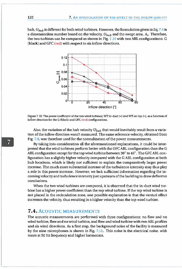
120 7. AN INVES’i IGATION ON THE EFFECT OF THE INFLOW QUALITY

hub, UJwb is different for both wind turbines. However, the formulation given in Eq. 7.4 isa dimensionless number based on the velocity, UInth and the swept area, A. Therefore,the two turbines can be compared as shown in Fig. 7.10 with two ABL configurations: G(black) and GFC (red) with respect to six inflow directions.

0.12

0.1

0.08

0.060

0.04

0.02

0

Figure 7.10: The power coefficient of the two wind turbines; WT in-duct (+) and WI on top (o), as a function ofinflow direction for the G (black) and GFC (red) configurations.

Also, the variation of the hub velocity Uj that would inevitably result from a variation of the inflow direction wasn’t measured. The same reference velocity, obtained fromFig. 7.9, was therefore used for the normalization of the power measurements.

By taking into consideration all the aforementioned explanations, it could be interpreted that the wind turbines perform better with the GFC ABL configuration than the GABL configuration except for the top wind turbine between 30° to 45°. The GFC ABL configuration has a slightly higher velocity compared with the G ABL configuration at bothhub locations, which is likely not sufficient to explain the comparatively larger powerincrease. The much more substantial increase of the turbulence intensity may thus playa role in this power increase. However, we lack sufficient information regarding the incoming velocity and turbulence intensity just upstream of the building to draw definitiveconclusions.

When the two wind turbines are compared, it is observed that the in-duct wind turbine has a higher power coefficient than the top wind turbine. If the top wind turbine isnot placed in the recirculation zone, one possible explanation is that the venturi effectincreases the velocity thus resulting in a higher velocity than the top wind turbine.

7.4. AcousTic MEASUREMENTS

The acoustic measurements are performed with three configurations; no flow and nowind turbine, flow and no wind turbine, and flow and wind turbine with two ABL profiles

and six wind directions. As a first step, the background noise of the facility is measuredby the nine microphones is shown in Fig. 7.11. This noise is the electrical noise, withtones at 50 Hz frequency and higher harmonics.

Inflow direction [°]

7.4. ACOUSTIC MEASUREMENTS 121

A-80

100102

[Hz]

Figure 7.11: PSD of all microphones in no flowconfiguration as a function of frequency.

Before investigating the noise characteristics of a wind turbine, the remaining system characteristics were analysed by removing the wind turbine. Figure 7.12 shows thePSD of each azimuthal microphones at three axial positions with the G and the GFC ABLconfigurations at 0° wind direction. The microphones at the azimuthal locations #2 and#3 show the same spectral shape, different from the results obtained at the azimuthallocation #1. It should be reminded that the microphones haven’t been calibrated in amplitude. When comparing the different ABE profiles with the same microphone, it isobserved that the amplitude of the PSD is higher with the GFC ABL configuration thanthe G ABL configuration. This can be related to the higher turbulence intensities.

With the wind turbines in place, the measured Blade Passing Frequency (BPF) forboth ABL configurations with six inflow directions have been obtained from the spectra(see Fig. 7.13 for the 00 deg wind direction), and have been gathered in Table 7.1. Whenthe inflow direction increases, the mass flow passing through the duct decreases, whichresults in a lower BPF except for the GFC ABE configuration at 15° wind direction. Inaddition, it is observed that the BPF difference between 0° and 15° wind direction arethe lowest compared to the other configurations. This effect might be due to the guidingeffect of the duct. For the two ABL configurations, it is observed that a higher BPF isobtained from the GFC ABL configuration. Figure 7.13(a) shows the position of the BPFfor the G ABE configuration, where half harmonics are also observed which may due tounequal spacing or the alignment of the wind turbine.

Table 7.1: Blade passing frequency values at all configurations

0° 15° 30° 45° 60 75°

G 433.57Hz 428.57Hz 394.56Hz 345.85Hz 301.43Hz 241.74Hz

GFC 528.19Hz 533.56Hz 473.88Hz 430.30Hz 370.36Hz 305.35Hz

Figure 7.13 shows the PSD of each azimuthal microphones at three axial position

-40

(C) Further downstream microphone configuration.

7. AN INVESTIGATION ON THE EFFECT OF THE INFLOW QUALITY

f[Hz]

(a) Upstream microphone configuration.

122

5’-20

G)

0C,)C-

5’-20

ci:;I

-40

0Cr)a-

5’-2o

ci)I

-40

0C’)a--

f[Hz]

(b) Downstream microphone configuration.

f[Hzj

Figure 7.12: PSD of the microphones without wind turbine at 00 inflow direction with two incoming flow; G(solid line) and GFC (dashed line), Microphones; # 1 (black), 2 (red) and 3 (green).

7.5. CONCLUSIONS 123

with and without wind turbine which were performed at Q0 wind direction with the GABL configuration. It can be seen that for the low frequency part the amplitude of thePSD is higher without the wind turbines than with them. This could be explained by alower velocity due to the wind turbine blockage within the duct. Furthermore, it is alsoobserved that the BPF and its harmonics are more pronounced upstream of the windturbine. The same figures are given for the GFC ABL configuration in Appendix C.3.

In order to compare the effects of the two ABL configurations, the results for microphone # 3 is selected at 0° wind direction and are shown in Fig. 7.14. A broadening ofthe BPF tones is observed with the GFC ABL configuration due to an increase in the turbulence intensity. The amplitude difference is not significant for the upstream locationfor frequencies below the first BPF where the harmonics are still present. For higherfrequencies, the broadband noise shows that the amplitude is higher for the GFC ABLconfiguration, which might be due to higher velocity as well as higher turbulence intensity. The downstream and further downstream positions show a significant amplitudeaugmentation for the lower frequencies, and they show another peak trend which is different from the upstream locations. Those peaks are not aligned with BPF and changewith the ABL configuration.

The effects of changing the wind direction are given in Fig. 7.15 for microphones #3 inthe GFC ABL configuration. In order to observe the trend with respect to the wind direction change, three values are selected; 00 (black), 30° (red) and 60° (green). It has beenobserved that the BPF decreases with increasing wind direction. The half harmonics ofthe BPF which were observed are now found to be less pronounced with the wind direction above 30°. However, the BPF amplitude and the PSD amplitude itself, increasedwith a higher inflow direction, especially for the broadband noise for the upstream microphone which could be due to the increase in the T.I. For the downstream and furtherdownstream positions, again a similar behavior is observed: an increase in the amplitude before the BPF and after the BPF, the amplitude of the spectrum almost remainsthe same for different inflow directions, This might be associated with the stall self-noise where the large coherent eddies emit the noise at a lower frequency. In addition,the tonal peaks are those which are observed in the previous figure and show that thosepeaks are independent on the flow conditions and the duct characteristics, which mightbe due to the electrical or mechanical noise.

7.5. CONCLUSIONSIn this section, a preliminary experimental study has been performed to investigate theeffect of the inflow quality on the power produced and noise emitted by a Building Integrated Wind Turbine (BIWT). The building model is selected from a previous study 11411which is a 1/200 scaled down model of Brussels Finance Tower, and a straight ductmodel, where the wind turbine is placed inside the duct. In addition, to investigate thebenefits of the BIWT installation locations, another wind turbine is placed on the top ofthe building.

As the focus of the current research is to investigate the effects of the quality anddirection of the flow on wind turbine performance and acoustic emission rather than toquantify the ABL type, two different neutral Atmospheric Boundary Layer (ABL) profilesare regenerated from a previous study [421. These inlet profiles in the VKI Li-B wind

124 7. AN INVESTIGATION ON THE EFFECT OF THE INFLOW QUALI’I V

tunnel are the only with Grid (G) and with Grid+Fence+Cups (GFC) configurations. Bothprofiles provide a similar velocity profile which changes by around 0.4m/s, while theturbulence intensity (T.I.) increases significantly with the GFC configuration; around 7%for the in-duct wind turbine compared to 3% for the top wind turbine. To vary the inflowdirection, six wind directions from 0° to 75° are performed by rotating a turntable whichthe building model is placed on.

The power coefficient, which is non-dimensionalized by the swept area of the windturbine and the velocity at the hub, is higher when the T.I. is increased except for the topwind turbine between 30° and 45° inflow direction. It is also observed that the top windturbine seems more insensitive to the T.I. than the in-duct wind turbine. Overall, whenthe two wind turbines are compared, the in-duct wind turbine produces more powerthan the top wind turbine.

The acoustic measurements are performed by nine microphones placed in three axial positions; upstream, downstream, and further downstream and three microphonesin each axial location. The measurements are performed with and without the windturbine, where it is observed that the amplitude of the spectrum decreases when thewind turbine is present due to the blockage effect. It is also observed that the turbulenceinteraction noise is more dominant on the upstream location than the other locationssince the Blade Passing Frequencies (BPF) and its harmonics are only observed in theupstream position, while the peaks are attenuated while moving downstream; only theBPFs which have more energy content remain. The comparison of the incoming flowis investigated by one azimuthal location along the three axial positions as a functionof frequency divided by BPF. It is observed that the peaks obtained from the GFC ABLconfiguration are wider and their peak points are more rounded than the G ABL configuration. Moreover, the small peaks observed from the G ABL configuration, which mightbe due to misalignment of the wind turbine or unequal blades, are suppressed by thenoise which results in smoother peaks. When different axial locations are investigated,similarly, the BPF and its harmonics are more present in the upstream microphone position than the downstream ones. Moreover, the amplitude difference and the width of thepeaks are wider for the downstream locations. As a last step, the inflow direction variation was investigated by considering only three angles 0°, 30° and 60° wind directionsfor one azimuthal location along three axial positions. As expected, increasing the winddirection reduced the velocity, and thus the BPF and its harmonics shift to left. Moreover, two different behaviors are observed depending on the axial location. With respectto the upstream microphone, the low frequency range seems less effected by the wind direction, however, a broadband noise increase is observed for the higher frequencies. Onthe contrary, the downstream microphones seem more sensitive to the inflow directionfor the low frequency range than the higher frequencies.

In future work, the ABL profile could be obtained when the building is present withdifferent wind directions. to investigate the blockage effect of the model and properlyobtain the inlet velocity. Furthermore, to better understand the flow field around andinside the duct, a Particle Image Velocimetry (PIV) measurement could be performed.This would give more information about the separation due to the sharp edge of the ductand the building, as well as the vortices formed due to tip leakage. Lastly, a microphonecalibration would help to more quantify and characterize the noise emitted by the wind

7.5. CONCLUSIONS 125

turbine and the in-duct model decomposition technique could be applied to investigatethe propagation of the acoustic waves inside the duct.

126 7. AN INVESTIGATION ON THE EFFECT OF THE INFLOW QUALITY

5’-20

F::

5’ -20

5’-20

F::(C) Further downstream microphone configuration.

Figure 7.13: PSD comparison with and without wind turbine at 00 wind direction for the G ABL configuration;with wind turbine (solid line) and without wind turbine (dashed line), Microphones; # 1 (black), 2 (red) and 3

f[Hz]

(a) Upstream microphone configuration.

f[Hz]

(b) Downstream microphone configuration.

f[Hz]

(green).

7.5. CONCLUSIONS 127

5’ -20

-40

(I) -60

5’-20

a)

-40

ci) -60

5’ -20

a)I

-40

C(I) -60

f/BPF [-](a) Upstream microphone #3.

11f/BPF [-]

(b) Downstream microphone #3.

1( 1(fIBPF [-1

(c) Further downstream microphone #3.

Figure 7.14: PSD comparison of microphones #3 with respect to incoming flow; G C—) and GFC (—).

128 7. AN INVESTIGATION ON THE EFFECT OF THE INFLOW QUALITY

5’ -20

F::

5’ -20

5’ -20

a)

-40

(I)U--

Figure 7.15: PSD comparison of microphones #3 with and without wind turbine with the GFC ABL configuration at different wind directions; with wind turbine (solid line) and without wind turbine (dashed line), 00

(black), 300 (red) and 60° (green).

f[Hz]

(a) Upstream microphone #3.

f[Hz]

(b) Downstream microphone #3.

f[Hz]

(c) Further downstream microphone #3.

CONCLUSIONS

This chapter focuses on the summary of the thesis with its main results followed by thefuture work and further improvements.

8.1. SUMMARY AND MAIN RESULTSIn this study, the noise emitted by a ducted wind turbine is investigated both numerically and experimentally. The numerical part, which is denoted as Part I, focuses onthe accuracy, validation and development of low cost methods to predict the far-fieldtrailing edge noise. To achieve this, Amiet’s theory, which relates the statistical description of the pressure field beneath the incoming turbulent boundary layer to the acousticfield, is applied. The state-of-art wall-pressure models are tuned based on RANS simulations and their accuracy with respect to the different mesh resolutions is investigatedfor an isolated airfoil. Further analyses are performed on a full scale of a commercialducted wind turbine by neglecting the scattering due to the diffuser. As a final step, toreduce the computational time, a 2D approach based on the strip theory is applied. Theacceleration due to the diffuser and nacelle is imposed as an inlet condition which isobtained from a 2D axisymmetric simulation without blade. In the experimental part,two different aspects are investigated. First, the development of a remote microphonemeasurement technique which can be placed on the duct surface in order to acquire thenoise emitted by rotating machines is proposed. Second, the effect of the aerodynamicroughness on the noise emission is evaluated for a building-integrated wind turbine.Furthermore, the suitable siting position of a wind turbine is investigated by comparingthe power efficiency of a wind turbine within a duct and on the top of the building.

The far-field trailing edge noise is predicted by Amiet’s theory for NACAOO12 andDU96-W-180 airfoils at 00 and 4° angle of attacks, respectively, in Chapter 4. 2D HANSsimulations are performed by the k —12 SST turbulence model and the turbulent boundary layer profiles are extracted at x/c = 0.99 from the leading edge. The wall-pressurespectrum is computed by semi-empirical models which are Goody (assuming ZPG),Rozenberg, Kamruzzaman, Catlett, Ru & Herr and Lee (assuming APG) and an integral

129

130 8. CoNclusioN

method (Panton & Linebarger). The grid sensitivity analysis is performed for both airfoils with different grid resolutions characterized by the non-dimensional wall-normalunits, Overall, the pressure coefficient for both airfoils shows mesh independentresults whereas the turbulent boundary layer profiles in terms of the wall-normal velocity (only for the DU96-W-180 airfoil), the kinetic energy and the specific dissipationfor both airfoils exhibit some sensitivity with respect to the mesh resolution. The wall-pressure spectrum obtained by the semi-empirical models are insensitive to the meshresolution, while the spectrum obtained by the Panton & Linebarger model performsmesh independence for y <5 for the NACAOO12 airfoil. When the wall-pressure spectrum is compared with the NACAOO12 airfoil experimental data, it is concluded that theGoody model is not accurate for the APG flow. Even though, the Cattlett and Hu & Herrmodels are developed forAPG flows, a poor prediction is observed, which can be relatedto the scaling of the flat-plate experimental data. For the DU96-W-180 airfoil, it is concluded that the suction side, which contributes to the low frequency of the spectrum, ismore mesh-dependent than the pressure side which dominates the higher frequencies.A mesh independent solution for these airfoils and the flow solver is obtained for y <15for kc> 10. Moreover, the Kamruzzaman and the Panton & Linebarger models are foundto be generally applicable. When the probe location is varied along the trailing edge, it isconcluded that the far-field noise predictions by the semi-empirical models are sensitiveto the probe location for kc < 10.

As a next step, a full scale of a commercial ducted wind turbine is simulated by 3Dincompressible HANS with the k — 2 SST turbulence model in Chapter 5. The Coriolis and centrifugal effects are considered by applying a MRF methodology. The far-fieldtrailing edge noise is predicted by applying the Schlinker and Amiet theory. Pm alternative approach based on a 2D strip theory is proposed to reduce the computationaltime required for the 3D HANS simulation. In this method, the blade is divided intostrips and 2D RANS simulations are performed for each strip location to obtain the turbulent boundary layer near the trailing edge. A further improvement of this method isintroduced by taking into account the acceleration due to the diffuser and nacelle. Thisis achieved by extracting the axial velocity profiles from a 2D axisymmetric simulationwithout blade and imposing these profiles as the inlet conditions to the 2D strip simulations. Even though the comparison between the 3D simulation and 2D simulations obtained by the improved inlet conditions demonstrates a close match with respect to theaxial velocity extracted upstream of the blades, the azimuthal velocity and the pressurecoefficient exhibit a poor match. The same observation was made regarding the turbulent boundary layer profiles extracted at x/c = 0.99. In general, the wall-pressure spectrum obtained by the Panton & Linebarger model from the 3D simulation show lowerlevels than other models both for the 2D and 3D simulations. This might be due to thefact that the kinetic energy is under-predicted. The far-field noise prediction obtainedby the Kamruzzamari model imposing the inlet velocity at z/c —5.0 agrees well withthe 3D simulation at higher frequencies. In terms of the computation cost, the 2D simulations with the acceleration correction is about two orders of magnitude faster thancorresponding 3D simulations.

The development of a measurement device based on a remote microphone is introduced in Chapter 6.2. The main purpose of this fairing is to enable the acquisition of

8.2. FUTURE RESEARCH AND POSSIBLE FURTHER IMPROVEMENTS 131

the noise emitted by rotating machines where the duct surface cannot be altered. Thedevice is designed using a streamlined profile, where the microphone is connected tothe surrounding with a pipe-cavity system. An analytical model is used to design thepipe-cavity system. However, the model deviates significantly compared to the responsefunction of the signal. The aim of the streamlined design is not to disturb the flow and tomake use of local acceleration which would reduce the turbulence level on the pressuretap and that would increase the noise to signal ratio. However, it is found that near-wallturbulence significantly increases when the incoming turbulence level is high. Contraryto this, a practical application where noise emitted by a contra-rotating fan is measured,the fairing and a free-field microphone reveals a good match.

In Chapter 7, a preliminary experimental study is conducted to investigate the effectof inflow conditions, in terms of wind speed and direction, on the power production andthe noise emission of a BIWT through a duct. Two different neutral ABL profiles, corresponding to different aerodynamic roughness lengths and turbulence intensities, areimposed as inlet profiles. Furthermore, another wind turbine is placed on the top of thebuilding to assess the best siting within the building by comparing the power efficiency.Although the two ABL configurations provide a similar velocity profile, the turbulenceintensity obtained by the GFC configuration is 7% and 3% higher than the G configuration for the in-duct and top wind turbine, respectively. It is concluded that the powerproduced by the in-duct wind turbine is higher than the top wind turbine while the topwind turbine appears to be less sensitive to the inflow direction than the in-duct windturbine. From the noise measurements obtained within the duct demonstrate that theturbulence interaction noise is more dominant upstream of the wind turbine than downstream. Furthermore, broad peaks are observed when the turbulence level is higher andwith higher magnitudes.

8.2. FUTURE RESEARCH AND POSSIBLE FURTHER IMPROVE

MENTS

Reminding that the grid sensitivity study is investigated using only one eddy-viscositymodel, k — 2 SST, further analysis with different turbulence models and numericalschemes would be recommended.

As the Corcos model is not physically consistent in the low-frequency regime, moreaccurate models such as Efimstsov and Smolyakov could be used to calculate the far-field spectrum.

When performing the 2D strip theory, only the axial acceleration is taken into account by applying a correction from a 2D axisymmetric simulation. However, the comparison with the 3D simulation exhibits a significant different when the azimuthal axialproffles are compared. Therefore, an analysis could be also performed by changing therotational speed to take the three-dimensional effects into account.

In literature, there are several correction for BEM to take into account the threedimensional effects. So that the inlet conditions acquired with a BEM method can beimposed to the 2D strip theory simulations to parametrize the 3D effects for a 2D simulation.

Further verification experiments can also be performed to test the consistency be-

132 8. CoNcLusioN

tween the reproduced inflow conditions at the Li wind tunnel with and without a building.

In this study, two wind turbines with the same blade design are used. However, theblades of the ducted wind turbine is cut in order to sit inside the building. Therefore,another possible future study can focus on the performance comparison of identicalwind turbines.

GLOBAL BOUNDARY LAYER

VARIABLES WITH RESPECT TO

PROBE LOCATION

133

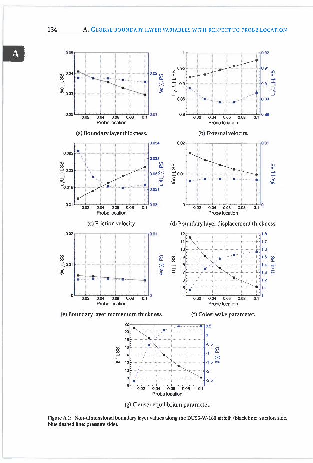
Sd

[-1“flI°fl

Sd

[-1/,9

C)C

0.2

t3.C_C

—o

C)

.0

71CUCccccccCccCCHHc_cccC”

C/i

ccccCHC/i

cccccccccccc>->-ccC71CCcc-IccCccC

C0C)00a)-o0a-

C0C)00a).00cc

C)C)2C)CC)0C)

ccC)CC)C)Cc_-c

C-

Sd’I-1

CC)CC?

bo

Cl?(C)C)0ccC

.)

c.0

0—C)

o3..

oC)

a)cc9C

)cc

CCccC)

C)

-C0CC-)CC

)CccC_CC)

ccCC)0C

)

I!4.2C(9OC

)

0-

.2C)

C)C

-C)

CCC)

C)

C““

a3-

C)cc

-CCC0ccC

)

.2-cc

oà-5C

Czcc-CC

)

<C

)

St

CC

)C-c

Ccc

cc

C_C

2.2

C)

C)C

)3-

0C.2C)

55

‘[-13/9

C0C)

00C)

.00cc

(C)

(C)

C)CccC-)

-C2CCC)

9CSC-

C)

C)

-CCCCccC)

55

‘[-]¶1

A

55

‘[-13/9

BOUNDARY LAYER PROFILES FROM

B.1. MESH SENSITIVITY

3D SIMULATION

The wail-normal and spanwise velocity profiles extracted at x/c 0.99 from the leadingedge with respect to the different mesh resolution are given as:

(b) Strip 2.

Figure B.1: The wall-normal velocity profiles at x/c =0.99 from the leading edge at each strip location withdifferent mesh resolutions; Yve 2.5 () Yave 2 ( — ), Yave 1.6 ( —

0.

0.1

0

0.05

0 0.02 0.04 0.06 0.08 0.1

V/UReI 1](a) Strip 1.

V/Uei [] V/UReI [1

(C) Strip 3.

135

136 B. BOUNDARY LAYER PROFILES FROM 3D SIMULATION

0.05 0.1 0.01 0.01

\N/UReI [j W/U [-] N/Uei []

(a) Strip 1. (b) Strip 2. (C) Strip 3.

Figure B.2: The spanwise velocity profiles at x/c 0.99 from the leading edge at each strip location with different mesh resolutions; Yave 2.5 (), Yave 2 ( — ), Yave 1.6 ( —

B.2. BOUNDARY LAYER COMPARISON BETWEEN 2D AND 3D

SIMULATIONSThe comparison of the kinetic energy proffle and the specific dissipation rate extractedat x/c = 0.99 from the leading edge with 2D and 3D simulations is given in Fig. B.3 andFig. B.4.

B.3. GLOBAL BOUNDARY LAYER VARIABLESThe global boundary layer variables obtained from 2D and 3D simulations are given inthe following table.

- 0.002 0.004 0.006 0.008 0.01 0.012

k/1Jei []

(a) Strip 1.

0.15 — —

0.1

C.)>

0.05

0.002 0.004 0.006 0.008 0.01 0.012

ki/Uei [1

(C) Strip 5.

Figure B.3: The turbulent kinetic energy profiles extracted at x/c = 0.99 with respect to each strip location;C— — -) U21_05 (— —) Uj0667 C ) and 3D simulation ()

El

B.3. GLOBAL BOUNDARY LAYER VARIABLES

__________________________

137

C-)>

0.1

C-)>

0.05

0.004 0.006 0.008 0.01 0.012

ki/Ue []

(b) Strip 3.

138 B. BOUNDARY LAYER PROFILES FROM 3D SIMULATION

0

QC/UReI []

(c) Strip 5.

Figure B.4: The specific dissipation profiles extracted at x/c = 0.99 with respect to each strip location;

(—), U4_5O (— — -) (— — ) ( ) and 3D simulation (°).

OC/U5ei [] OC/UReI [1

(a) Strip 1. (b) Strip 3.

B.3. GLOBAL BOUNDARY LAYER VARIABLES 139

II

Table B.1: Global variables at x/c = 0.99 for Uq066.

Simulation Side Strip number ö/c (Jp/Uei Lty/Up1 6*/c 8/c U 13

Stripi - - - - - - -

Strip2 - - - - - - -

Suction Strip 3 - - - - - - -

Strip4 0.043 1.020 0.001 0.016 0.007 0.9827 0.8155

Strip5 0.042 1.001 0.001 0.015 0.007 1.2324 1.2792UZ/(=O.6S7

Strip 1 0.010 1.737 0.019 0.002 0.001 0.2606 -0.2758

Strip2 0.009 1.461 0.008 0.002 0.001 - -0.6291

Pressure Strip3 0.014 1.075 0.004 0.003 0.002 0.0675 -0.463

Strip 4 0.016 1.002 0.002 0.003 0.002 0.1927 -0.3501

Strip5 0.015 0.985 0.002 0.003 0.002 0.2203 -0.3208

BUILDING INTEGRATED WIND

TURBINE

The details about the Building Integrated Wind Turbine (BIWT) model is given. Themodel consists of three main modules; building, duct and wind turbine modules.

C.1. BUILDING INTEGRATED WIND TURBINE MODEL

C.1.1. BUILDING MODULEThe building model which is a 1/200 scale model of Brussels Finance Tower. The façadeplate and interior of the module is shown.

Figure C. 1: Building part with and without façade plate and movable duct part.

C.1.2. DUCT MODULEThe duct module is used to adjust the height of the system and dismantle the wind turbine.

141

142 C. BUILDING INTEGRATED WIND TURBINE

Figure C.2: Dismantling mechanism of duct module from building module.

C.1.3. WIND TURBINE MODULE

The duct module is used to adjust the height of the system and dismantle the wind turbine.

Figure C.3: Dismantling mechanism of duct module from building module.

C.2. POWER MEASUREMENTS

The electrical board shown in Fig. C.4 is used to perform the power measurements.

Applied Load

Figure C.4: The control board for wind farm (left), control board module (middle) and electrical resistance(right) [141].

C.3. ACOUSTIC MEASUREMENTS 143

C.3. ACOUSTIC MEASUREMENTSThe comparison of PSD with and without wind turbine at 0° a.o.a with GPC ABL configuratlonis given InFlg.C.5.

The effect ofa.o.als given In Fig. C.6 with GABL configuration comparing the microphones at #3 axIal position.

144 C. BUILDING INTEGRATED WIND TURBINE

5 -20

I:::5 -20

a)I

-40

U)

5-20

I-40

ci)0

Figure C.5: Comparison of the PSD with and without wind turbine at 00 inflow direction with GFC ABE configuration; with wind turbine (solid line) and without wind turbine (dashed line), Microphones; number 1 (black),2 (ted) and 3 (green).

f[Hzj

(a) Upstream microphone configuration.

f[Hz]

(b) Downstream microphone configuration.

f[Hz]

(c) Further downstream microphone configuration.

C.3.AcousTlc MEASUREMENTS 145

5-20

-40

0U)C-

5’-20

F::

5’-20

F::(C) Further downstream microphone #3.

Figure C.6: PSD comparison of microphones # 3 with and without wind turbine with G ABL configuration atdifferent inflow directions; with wind turbine (solid line) and without wind turbine (dashed line), 0° (black),30° (Led) and 60° (green).

f[Hzj

(a) Upstream microphone #3.

f[Hzl

(b) Downstream microphone #3.

f[Hz]

146 REFERENcES

REFERENCES[1] Abe, K., Nishida, M., Sakural, A., Ohya, Y., Kihara, H., Wada, E., Sato, K., 2005.

Experimental and numerical investigations of flow fields behind a small wind turbine with a flanged diffuser. Journal of Wind Engineering and Industrial Aerodynamics 93 (12), 951 —970.

[2] Abe, K., Ohya, Y., 2004. An investigation of flow fields around flanged diffusersusing CFD. Journal of Wind Engineering and Industrial Aerodynamics 92 (3), 315—330.

[3] Al-Kodmany, K., 2014. Green towers and iconic design: cases from three continents. Archnet-IJAR: International Journal of Architectural Research 8 (1), 11—29.

[4] Al-mulali, U., Fereidouni, H. G., Lee, J. Y., Sab, C. N. B. C., 2013. Exploring the relationship between urbanization, energy consumption, and C02 emission in MENAcountries. Renewable and Sustainable Energy Reviews 23, 107—112,

[5] Amiet, R., 1975. Acoustic radiation from an airfoil in a turbulent stream. Journal ofSound and Vibration 41(4), 407—420.

[6] Arniet, R., 1976. Noise due to turbulent flow past a trailing edge. Journal of Soundand Vibration 47 (3), 387—393.

[7] Amiet, R., 1977. Noise produced by turbulent flow into a propeller or helicopterrotor. AIAA Journal 15 (3), 307—308.

[8] Arniet, R., 1978. Effect of the incident surface pressure field on noise due to turbulent flow past a trailing edge. Journal of Sound and Vibration 57 (2), 305—306.

[9] Anselmi, L., 2017. Computational analysis of ducted wind turbines noise. Master’sthesis, Delft University of Technology.

[10] Antonini, C., Persico, G., Rowe, A. L., 2008. Prediction of the dynamic responseof complex transmission line systems for unsteady pressure measurements. Measurement Science and Technology 19 (12), 125401.

[11] Aranake, A., Duraisamy, K., 2017. Aerodynamic optimization of shrouded windturbines. Wind Energy 20 (5), 877—889.

[12] Aranake, A. C., Lakshminarayan, V K., Duraisamy, K., 2014. Assessment of low-order theories for analysis and design of shrouded wind turbines using CFD. Journal of Physics: Conference Series 524 (1), 012077.

113] Aranake, A. C., Lakshminarayan, V K., Duraisamy, K., 2015. Computational analysis of shrouded wind turbine configurations using a 3-dimensional RANS solver.Renewable Energy 75, 8 18—832,

[14] Arguillat, B., 2006. Étude expérimentale et numérique de champs depression pariétale dans l’espace des nombres d’onde, avec application aax vitrages automobiles. Ph.D. thesis, Ecole Centrale de Lyon.

REFERENCES 147

[15] Avallone, F, van der Velden, W, Ragni, D., 2017. Benefits of curved serrationson broadband trailing-edge noise reduction. Journal of Sound and Vibration 400,167-477.

[16] Bak, C., Johansen, J., Anderse, P B., 2006. Three-dimensional corrections of airfoilcharacteristics based on pressure distributions. In: European Wind Energy Conference & Exhibition (EWEC). Athens, Greece.

[171 Bakker, R., Pedersen, E., van den Berg, G., Stewart, R., Lok, W, Bouma, J., 2012.Impact of wind turbine sound on annoyance, self-reported sleep disturbance andpsychological distress. Science of The Total Environment 425, 42—5 1.

[18] Bangga, G., Lutz, T., lost, E., Kramer, E., 2017. CFD studies on rotational augmentation at the inboard sections of a 10 MW wind turbine rotor. Journal of Renewableand Sustainable Energy 9 (2), 023304.

[19] Barlas, E., 2014. Experimental investigation of wind turbine / farm wakes in aboundary layer wind tunnel. Master’s thesis, von Karman Institute for Fluid Dynamics,

[20] Barone, M. F, 2011. Survey of techniques for reduction of wind turbine blade trailing edge noise.

[21] Bergh, H., Tijdeman, H., 1965. Theoretical and experimental results for thedynamic response of pressure measuring systems. Technical Report. NationalAerospace Laboratory.

[22] Bertagnolio, F, 2008. Trailing edge noise model applied to wind turbine airfoils.Constraints 4, 0—002.

[23] Betz, A., 1920. Das maximum der theoretisch moglichen ausnutzung des windesdurch windmotoren. Zeitschrift für das gesamte Turbinenwesen 26, 307—309.

[24] Betz, A., 1929. Energieumsetzungen in venturidüsen. Naturwissenschaften17 (10), 160—164.

[25] Blake, W K., 1986. Mechanics of flow-induced sound and vibration Volume I, General concepts and elementary sources. Academic Press.

[26] Blandeau, V P, Joseph, P E, 2011. Validity of Amiet’s model for propeller trailingedge noise. AIAA Journal 49 (5), 1057—1066.

[27] Bontempo, R., Cardone, M., Manna, M., Vorraro, G., 2014. Ducted propeller flowanalysis by means of a generalized actuator disk model. Energy Procedia 45, 1107— 1115, aTI 2013 - 68th Conference of the Italian Thermal Machines EngineeringAssociation.

[28] Bontempo, R., Manna, M., 2014. Performance analysis of open and ducted windturbines. Applied Energy 136, 405—416.

148 REFERENCEs

[29] Bowdier, R., Leventhall, G., 2012. Wind turbine noise. Multi-Science Publishing CoLtd.

[30] Bree, H.-E. d., Eerden, F v d., Honschoten, I. v., 2000. A novel technique for measuring the reflection coefficient of sound absorbing materials.

[31] Brooks, T., Pope, D., Marcolini, M., 1989. Airfoil self-noise and prediction. NASAreference publication. National Aeronautics and Space Administration, Office ofManagement, Scientific and Technical Information Division.

[32] Buckingham, 5., 2010. Wind park siting in complex terrains assessed by wind tunnel simulations. Master’s thesis, von Karman Institute for Fluid Dynamics.

1331 Caetano Alves, J., 2005. Premesys v2.0: a software tool to characterize the dynamicresponse of apressure measurement system.

[34] Campbell, N., Stankovic, 5., 1999. Wind Energy for the Built Enviroment (ProjectWEB). Tech. rep.

[351 Campbell, N., Stankovic, S., M. Graham, P fl, van Duijvendijk, M., de Gruiter, T.,Behling, S., J. Hieber, M. B., 2001. Wind energy for the built enviroment (projectweb). In: European Wind Energy Conference & Exhibition. Copenhagen.

[36] Carcangiu, C. E., Sorensen, I. N., Cambuli, F, Mandas, N. 2007. CFD—RANS analysisof the rotational effects on the boundary layer of wind turbine blades. Journal ofPhysics: Conference Series 75, 012031.

[37] Casalino, D., Barbarino, M., 2011. Stochastic method for airfoil self-noise computation in frequency domain. AIAA Journal 49 (11), 2453—2469.

[38] Catalano, P, Amato, M., 2003. An evaluation of PANS turbulence modelling foraerodynamic applications. Aerospace science and Technology 7 (7), 493—509.

[39] Catlett, M. R., Anderson, J. M., Forest, J. B., Stewart, D. 0., 2015. Empirical modeling of pressure spectra in adverse pressure gradient turbulent boundary layers.ALAA Journal 54 (2), 569—587.

[40] Chandiramani, K. L., 1974. Diffraction of evanescent waves, with applications toaerodynamically scattered sound and radiation from unbaffled plates. The Journalof the Acoustical Society of America 55 (1), 19.

[41] Chase, D., 1980. Modeling the wavevector-frequency spectrum of turbulentboundary layer wall pressure. Journal of Sound and Vibration 70 (1), 29—67.

[42] Chauveau, M., 2017. Instantaneous measurements of fluctuating temperature andvelocity Master’s thesis, von Karman Institute for Fluid Dynamics.

[43] Chaviaropoulos, P, Hansen, M., 2000. Investigating three-dimensional and rotational effects on wind turbine blades by means of a quasi-3D Navier-Stokes Solver.Journal of Fluids Engineering 122, 330—336.

REFERENcEs 149

[44] Chitale, K. C., Rasquin, M., Sahni, 0., Shephard, M. S., Jansen, K. E., 2014. Boundary layer adaptivity for incompressible turbulent flows. ArXiv e-prints.

[45] Christophe, J., Moreau, S., Hamman, C. W, Witteveen, I. A. S., laccarino, G., 2014.Uncertainty quantification for the trailing-edge noise of a controlled-diffusion airfoil. AIAA Journal 53 (1), 42—54.

[46] Clauser, E H., 1954. Turbulent boundary layers in adverse pressure gradients. Journal of the Aeronautical Sciences 21(2), 91—108.

[47] Coles, D., 1956. The law of the wake in the turbulent boundary layer. Journal ofFluid Mechanics 1(2), 191—226.

[48] Conan, B., 2012. Wind resource assesment in complex terrain by wind tunnel modelling. Ph.D. thesis, Université d’Orléans.

[49] Corcos, G. M., 1964. The structure of the turbulent pressure field in boundary-layerflows. Journal of Fluid Mechanics 18 (03), 353.

[50] Coudou, N., 2016. Wind turbine / farm wake(s) meandering study in an ABL tunnel. Master’s thesis, von Karman Institute for Fluid Dynamics.

[51] Curle, N., 1955. The influence of solid boundaries upon aerodynamic sound. Proceedings of the Royal Society A: Mathematical, Physical and Engineering Sciences231 (1187), 505—514.

[52] Dayan, E., 2006. Wind energy in buildings. Refocus 7 (2), 33—38.

[53] Degrassi, S., Castelli, M. R., Benini, E., 2013. A retrospective of wind turbine architectural integration in the built environment. World Academy of Science, Engineering and Technology International Journal of Civil, Environmental, Structural,Construction and Architectural Engineeringy7 (6), 417—421.

[54] der Luft im VDI und DIN. Normenausschuss, K. R., 2000. Environmental meteorology: physical modelling of flow and dispersion processes in the atmosphericboundary layer: application of wind tunnels:. DIN-VDI-Taschenbuch. Beuth Verlag.

[55] Dick, E., 1986. Power limits for wind energy concentrator systems. Wind Engineering 10 (2), 98—115.

[561 Dighe, V, Avalione, E, van Bussel, G., 2016. Computational study of diffuser augmented wind turbine using actuator disc force method. International Journal ofComputational Methods and Experimental Measurements 4 (4), 522—53 1.

[571 Dighe, V V, Avallone, E, Tang, I., van Bussel, G., Jan 2017. Effects of gurney flapson the performance of diffuser augmented wind turbine. American Institute ofAeronautics and Astronautics.

[581 Doolan, C., 2013. A review of wind turbine noise perception, annoyance and lowfrequency emission. Wind Engineering 37 (1), 97—104.

150 REFERENcEs

[59] Doolan, C. I., Gonzalez, C. A., Hansen, C. H., 2010. Statistical estimation of turbulent trailing edge noise. In: Proceedings of 20th International Congress on Acoustics. American Institute of Aeronautics and Astronautics.

[60] Doolan, C. I., Moreau, D. J., Brooks, L. A., 2012. Wind turbine noise mechanismsand some concepts for its control. Acoustics Australia 40 (1).

[61] Drela, M., 1989. Xfoil: An analysis and design system for low Reynolds number airfoils. In: Mueller, T. J. (Ed.), Low Reynolds Number Aerodynamics. Springer BerlinHeidelberg, Berlin, Heidelberg, pp. 1—12.

[62] Du, Z., Selig, M., jan 1998. A 3-D stall-delay model for horizontal axis wind turbine performance prediction. In: 1998 ASME Wind Energy Symposium. AmericanInstitute of Aeronautics and Astronautics.

[63] Du, Z., Selig, M., 2000. The effect of rotation on the boundary layer of a wind turbine blade. Renewable Energy 20 (2), 167—181.

[64] Dumitrache, A., Cardos, V, Dumitrescu, H., Simos, T. F., Psihoyios, G., Tsitouras,C., 2010. Delayed stall modeling of the rotating blades. AlP.

[65] Dumitrescu, H., Cardos, V, 2009. Inboard boundary layer state on wind turbineblades. ZAMM-Journal of Applied Mathematics and Mechanics/Zeitschrift furAngewandte Mathematik und Mechanik 89 (3), 163—173.

1661 Dumitrescu, H., Cardos, V, 2012. Inboard stall delay due to rotation. Journal ofAircraft 49 (1), 101—107.

1671 Durbin, F, Reif, B., 2011. Statistical theory and modeling for turbulent flows. Wiley.

1681 E., L., 2011. Advanced cfd methods for wind turbine analysis. Ph.D. thesis, GeorgiaInstitute of Technology, Atlanta, GA, USA.

[69] Efimtsov, B., 1982. Characteristics of the field of turbulent wall pressure-fluctuations at large Reynolds-numbers. Soviet Physics Acoustics-USSR 28 (4),289—292.

[70] Ewert, H., 2007. RPM - the Fast Random Particle-Mesh Method to realize unsteady turbulent sound sources and velocity fields for CAA Applications. In: 13thAIAA/CEAS Aeroacoustics Conference (28th AIAA Aeroacoustics Conference).Vol. 4, American Institute of Aeronautics and Astronautics, Reston, Virigina, p. 1.

[71] Ewert, R., 2008. Broadband slat noise prediction based on CAA and stochasticsound sources from a fast random particle-mesh (RPM) method. Computers &Fluids 37 (4), 369—387.

[72] Fletcher, C. A., 1981. Computational analysis of diffuser-augmented wind turbines. Energy Conversion and Management 21(3), 175— 183.

REFERENcEs 151

[73] Foreman, K., 1981. Preliminary design and economic investigations of Diffuser-augmented Wind Turbines (DAWT). Executive Summary. Final Report. NationalRenewable Energy Laboratory (U.S.).

[74] Garratt, J. R., 1994. The atmospheric boundary layer (Cambridge Atmospheric andSpace Science Series). Cambridge University Press.

[75] Giahi, M. H., Dehkordi, A. J., 2016. Investigating the influence of dimensional scaling on aerodynamic characteristics of wind turbine using CFD simulation. Renewable Energy 97, 162—168.

[76] Gilbert, B. L., Foreman, K. M., 1979. Experimental demonstration of the diffuser-augmented wind turbine concept. Journal of Energy 3 (4), 235—240.

[77] Gilbert, B. L., Oman, R. A., Foreman, K. M., 1978. Fluid dynamics of diffuser-augmented wind turbines. Journal of Energy 2 (6), 368—374.

[78] Gloerfelt, X., Le Garrec, T., 2009. Trailing edge noise from an isolated airfoil at ahigh Reynolds number. AIAA Journal.

[79] Goody, M., 2004. Empirical spectral model of surface pressure fluctuations. AIAAJournal 42 (9), 1788—1794.

[80] Grönman, A., Backman, I., Avramenko, A., 2014. Wind proffle effect on small windturbine noise generation. In: Volume 3B: Oil and Gas Applications Organic Rank-me Cycle Power Systems Supercritical C02 Power Cycles Wind Energy ASME.

[81] Guerri, 0., Bouhadef, K., Harhad, A., 2006. Turbulent flow simulation of the NRELS809 airfoil. Wind Engineering 30 (4), 287—301.

[82] Guidati, G., Barei, R., Wagner, 5., 1994. An investigation of blade-tower-interactionnoise (bti) for horizontal axis wind turbines in upwind and downwind configuration. first steps towards modeling of aeroelastic effects. In: Proc. 8th lEA Symposium. pp. 249—255.

[83] Guilmineau, E., Piquet, J., Queutey, P, 1997. Two-dimensional turbulent viscousflow simulation past airfoils at fixed incidence. Computers & Fluids 26 (2), 135—162.

[84] Gumley, 5., 1983. A detailed design method for pneumatic tubing systems. Journalof Wind Engineering and Industrial Aerodynamics 13 (1), 441 —452.

[85] H. Snel, R. Houwink, J. B., 1994. Sectional Prediction of Lift Coefficients on Rotating Wind Turbine Blades in Stall. Netherlands Energy Research Foundation.

[86] Hansen, C. H., Doolan, C. J., Hansen, K. L., 2017. Wind Farm Noise: Measurement,Assessment, and Control (Wiley Series in Acoustics Noise and Vibration). Wiley.

[87] Hansen, M., Sørensen, J., Voutsinas, S., Sorensen, N., Madsen, H., 2006. State ofthe art in wind turbine aerodynamics and aeroelasticity Progress in AerospaceSciences 42 (4), 285—330.

152 REFERENcEs

[88] Hansen, M. 0. L., 2008. Aerodynamics of Wind Turbines. Earthscan PublicationsLtd.

[89] Hansen, M. 0. L., Madsen, H. A., 2011. Review paper on wind turbine aerodynamics. Journal of Fluids Engineering 133 (11), 114001.

[90] Hansen, M. 0. L., Sorensen, N. N., Flay, R. G. 1., 2000. Effect of placing a diffuseraround a wind turbine. Wind Energy 3 (4), 207—213.

[911 Herr, M., Bahr, C. 1., Karnruzzaman, M., 2012. Problem Statement for theAJAA/CEAS Second Workshop on Benchmark Problems for Airframe Noise Computations (BANC-Il). ALAA Journal.

[921 Herr, M., Ewert, R., Rautmann, C., Kamruzzaman, M., Bekiropoulos, D., Anna, R.,Job, A., Batten, P, Chakravarthy, S., Bertagnolio, F, 2015. Broadband Trailing-EdgeNoise Predictions—Overview of BANC-Ill Results. In: 21st AJAA/CEAS Aeroacoustics Conference. American Institute of Aeronautics and Astronautics, Reston, Virginia.

[93] Herrig, A., Kamruzzaman, M., Würz, W, Wagner, 5., 2013. Broadband airfoiltrailing-edge noise prediction from measured surface pressures and spanwiselength scales. International Journal of Aeroacoustics 12 (1-2), 53—82.

[94] Himmelskamp, H., 1945. Profile investigations on a rotating airscrew. Ph.D. thesis,Gottingen University, Germany.

[951 Hirschberg, A., Rienstra, S. W, 2004. An introduction to aeroacoustics. Tech. rep.

[96] Holmberg, A., Abom, M., Bodén, H,, 2011. Accurate experimental two-port analysis of flow generated sound. Journal of Sound and Vibration 330 (26), 6336— 6354.

[97] Howe, M. S., 1998. Acoustics of Fluid-Structure Interactions. Cambridge UniversityPress, Cambridge.

[98] Hu, N., Herr, M., 2016. Characteristics of wall pressure fluctuations for a flat plateturbulent boundary layer with pressure gradients. In: 22nd AIAA/CEAS Aeroacoustics Conference. Aeroacoustics Conferences. American Institute of Aeronautics and Astronautics, p. 2749, 0.

[99] Hu, S.-Y., Cheng, 1.-H., 2008. Innovatory designs for ducted wind turbines. Renewable Energy 33 (7), 149 1—1498.

1100] Hurst, A. M., Van De Weert, 1., 2013. An experimental and theoretical investigationof wave propagation in teflon and nylon tubing with methods to prevent abasingin pressure scanners. Journal of Engineering for Gas Turbines and Power 135 (10),101602—101602.

11011 Hwang, Y., Bonness, W K., Hambric, S. A., 2009. Comparison of Semi-EmpiricalModels for Turbulent Boundary Layer Wall Pressure Spectra. Journal of Sound andVibration 319 (1), 199—217.

REFERENCES 153

[102] Igra, 0., 1976. Shrouds for aerogenerators. AIAA Journal 14 (10), 1481—1483.

[1031 Igra, 0., 1977. The shrouded aerogenerator. Energy 2 (4), 429—439.

[104] Igra, 0., 1981. Research and development for shrouded wind turbines. EnergyConversion and Management 21(1), 13— 48.

[105] Irwin, H., Cooper, K., Girard, R., 1979. Correction of distortion effects caused bytubing systems in measurements of fluctuating pressures. Journal of Wind Engineering and Industrial Aerodynamics 5 (1), 93— 107.

[106] Ishugah, T., Li, Y., Wang, R., Kiplagat, J., 2014. Advances in wind energy resourceexploitation in urban environment: A review. Renewable and Sustainable EnergyReviews 37, 6 13—626.

[107] Iwasaki, M., 1953. The experimental and theoretical investigation of windmills.Reports of Research Institute for Applied Mechanics 2 (8), 181—229.

[108] Jamieson, P M., 2009. Beating Betz: Energy extraction limits in a constrained flowfield. Journal of Solar Energy Engineering 131 (3), 031008—031008—6.

[1091 Jones, D. W, 1991. How urbanization affects energy-use in developing countries.Energy Policy 19 (7), 621—630.

[110] Kamruzzaman, M., Bekiropoulos, D., Lutz, T., Wflrz, W, Kramer, E., 2015. A semi-empirical surface pressure spectrum model for airfoil trailing-edge noise prediction. International Journal of Aeroacoustics 14 (5-6), 833—882.

[111] Kamruzzaman, M., Herrig, A., Lutz, T., Würz, W, Kramer, E., Wagner, S., 2011.Comprehensive evaluation and assessment of trailing edge noise prediction basedon dedicated measurements. Noise Control Engineering Journal 59 (1), 54.

[112] Kardous, M., Chaker, R., Aloui, F, Nasrallah, S. B., 2013. On the dependence of anempty flanged diffuser performance on flange height: Numerical simulations andPly visualizations. Renewable Energy 56, 123 — 128, the International Conferenceon Renewable Energy: Generation and Applications.

[113] Kiebanoff, P S., January 1955. Characteristics of turbulence in boundary layer withzero pressure gradient. Tech. rep.

[114] Kogan, A., Seginer, A., 1963. Final Report on Shroud Design. Tech, rep., Dept. ofAeronautical Eng.,.

[115] Kogan, A., Seginer, A., 1963. Shrouded Aerogenerator Desing Study II, Axisymmetnc Shroud Performance. Tech, rep., Dept. of Aeronautical Eng.,.

[116] Kraichnan, R. H., 1956. Pressure fluctuations in turbulent flow over a flat plate. TheJournal of the Acoustical Society of America 28 (3), 378—390.

154 REFERENcEs

[117] Kral, L., 1998. Recent experience with different turbulence models applied tothe calculation of flow over aircraft components. Progress in Aerospace Sciences34 (7), 481—541.

[118] Kucukcoskun, K., 2012. Prediction of free and scattered acoustic fields of low-speed fans. Ph.D. thesis, Ecole Centrale de Lyon.

[119] Lee, S., Villaescusa, A., 2017. Comparison and assessment of recent empiricalmodels for turbulent boundary layer wall pressure spectrum. In: 23rd AIAA/CEASAeroacoustics Conference. American Institute of Aeronautics and Astronautics, p.3688.

[1201 Lee, Y.-T., Blake, W K., Farabee, T. M., 2004. Modeling of wall pressure fluctuationsbased on time mean flow field. Journal of Fluids Engineering 127 (2), 233—240.

[121] Lewis, R. I., Williams, I. E., Abdelghaffar, M. A., 1977. A theory and experimentalinvestigation of ducted wind turbines. Wind Engineering 1, 104—125.

[122] Lighthill, M. 1., 1952. On sound generated aerodynamically. i. general theory. Proceedings of the Royal Society A: Mathematical, Physical and Engineering Sciences211 (1107), 564—587.

[123] Lighthill, M. J., 1954. On sound generated aerodynamically. II. turbulence as asource of sound. Proceedings of the Royal Society A: Mathematical, Physical andEngineering Sciences 222 (1148), 1—32.

[124] Lilley, G., Rainbird,W,Association, E. R., 1956.APreliminaryReport on the Designand Performance of Ducted Windmills. CoA report aero. College of Aeronautics.

1125] Lilley, G. M., Hodgson, T., 1960. On surface pressure fluctuations in turbulentboundary layers. Tech, rep., Advisory Group For Aeronautical Research and Development Paris(France).

[126] Lindenburg, C., 2004. Modelling of rotational augmentation based on engineeringconsiderations and measurements. In: European Wind Energy Conference. London, pp. 22—25.

[127] Loeffler, A. L., Steinhoff, J. 5., 1985. Computation of wind tunnel wall effects inducted rotor experiments. Journal of Aircraft 22 (3), 188—192.

[128] Loeffler, J. A. L., 1981. Flow field analysis and performance of wind turbines employing slotted diffusers. Journal of Solar Energy Engineering 103 (1), 17—22.

[129] Lowson, M. V, 1965. The sound field for singularities in motion. Proceedings ofthe Royal Society A: Mathematical, Physical and Engineering Sciences 286 (1407),559—572.

[130] Menter, F R., 1994. Two-equation eddy-viscosity turbulence models for engineering applications. AIAA Journal 32 (8), 1598—1605,

REFERENcEs 155

[131] Mertens, S., 2006. Wind Energy in the Built Environment: Concentrator Effects ofBuildings. Multiscience Publishing.

[1321 Moreau, A., Guerin, S., Enghardt, L., Denmat, A.-L. L., Nicke, E., Weber, S., Diehi,S., Koch, P, 2012.

[1331 Moreau, S., Roger, M., jan 2007. Competing broadband noise mechanisms in low-speed axial fans. AIAA Journal 45 (1), 48—57.

[134] Moriarty, R, Migliore, P G., (U.S.), N. R. E. L., 2003. Semi-empirical aeroacousticnoise prediction code for wind turbines [electronic resource] / P Moriarty and PMigliore. National Renewable Energy Laboratory Golden, Cob.

[135] Moshfeghi, M., Song, Y. J., Xie, Y. H., 2012. Effects of near-wall grid spacing onSST-k-w model using NREL phase VI horizontal axis wind turbine. Journal of WindEngineering and Industrial Aerodynamics 107-108, 94—105.

[136] Nash, J. F, 1966. Turbulent-Boundary-Layer Behaviour and the Auxiliary Equation.HM Stationery Office.

[137] Nations, U., 2007. City planning will determine pace of global warming.

[138] Oerlemans, S., Schepers, J. G., 2009. Prediction of wind turbine noise and validation against experiment. International Journal of Aeroacoustics 8 (6), 555—584.

[139] Ohya, Y., Karasudani, T., 2010. A shrouded wind turbine generating high outputpower with wind-lens technology. Energies 3 (4), 634—649.

[140] Ohya, Y., Karasudani, T., Sakurai, A., ichi Abe, K., Inoue, M., 2008. Development ofa shrouded wind turbine with a flanged diffuser. Journal of Wind Engineering andIndustrial Aerodynamics 96 (5), 524—539.

[141] Ozçakmak, 0. S., 2016. Building integrated wind turbines. Master’s thesis, von Karman Institute for Fluid Dynamics.

[142] Panton, R. L., Linebarger, J. H., 1974. Wall pressure spectra calculations for equilibrium boundary layers. Journal of Fluid Mechanics 65 (02), 261.

[143] Pape, A. L., Lecanu, J., 2004. 3D Navier-Stokes computations of a stall-regulatedwind turbine. Wind Energy 7 (4), 309—324.

[144] Parchen, R,, TNO-TH., T. P D., 1998. Progress report DRAW: a prediction schemefor trailing edge noise based on detailed boundary layer characteristics. TNOreport HAG-RPT. TNO Institute of Applied Physics.

[145] Park, J., Jung, H.-J., Lee, S.-W, Park, 1., 2015. A new building-integrated wind turbine system utilizing the building. Energies 8 (10), 11846—11870.

[146] Perea-Moreno, M.-A., Hernandez-Escobedo, Q., Perea-Moreno, A.-J., 2018. Renewable energy in urban areas: Worldwide research trends. Energies 11(3), 577.

156 REFERENcES

[147] Perennes, S., Roger, M., 1998. Aerodynamic noise of a two-dimensional wing withhigh-lift devices. In: 4th ALAA/CEAS Aeroacoustics Conference. p. 2338.

[148] Philips, D., 2003. An investigation on diffuser augmented wind turbine design.Ph.D. thesis, Unverstiy of Auckland.

[149] Phillips, D., Flay, R., Nash, T., 1998. Aerodynamic analysis and monitoring of thevortec 7 diffuser-augmented wind turbine. In: IPENZ Conference. Auckland, NewZealand.

[150] Phillips, D., Richards, P, G.D., M., Flay, R., 1998. Computational modelling of diffuser designs for a diffuser augmented wind turbine. In: 13th Australasian FluidMechanics Conference. Monash University, Melbourne, Australia.

[151] Pinder, 1., 1992. Mechanical noise from wind turbines. Wind Engineering 16 (3),158—168.

[152[ Ramachandran, R. C., Patel, H., Raman, G., Jiang, Y, Krishnamurthy, M., 2014.Noise source localization on a small wind turbine using a compact microphonearray with advanced beamforming algorithms: Part i — a study of aerodynamicnoise from blades. Wind Engineering 38 (1), 73—88.

[153] Redonnet, S., Jun. 2014. Aircraft noise prediction via aeroacoustic hybrid methods- development and application of onera tools over the last decade: some examples. AerospaceLab (7), p. 1—16.

[154] Remmler, S., Christophe, J., Anthoine, I., Moreau, S., 2010. Computation of wallpressure spectra from steady flow data for noise prediction. AIAA Journal 48 (9),1997—2007.

[1551 Roger, M., 2004. Noise from moving surfaces. In: Advances in aeroacoustics andapplications, von Karman Institute for Fluid Dynamics.

[1561 Roger, M., Moreau, S., 2005. Back-scattering correction and further extensions ofAmiet’s trailing-edge noise model. Part 1: theory. Journal of Sound and Vibration286 (3), 477—506.

[157j Rotta, J., 1953. On the theory of the turbulent boundary layer.

[158] Rozenberg, Y., 2007. Modélisation analytique du bruit aerodynamique a largebande des machines tournantes: utiisation de calculs moyennés de mécaniquedes fluides. Ph.D. thesis, Ecole Centrale de Lyon.

[159] Rozenberg, Y., Robert, G., Moreau, S., 2012. Wall-pressure spectral model including the adverse pressure gradient effects. AIAA Journal 50 (10), 2168—2179.

11601 Sack, S., Abom, M., Schram, C., Kucukcoskun, K., Jun 2014. Generation and scattering of acoustic modes in ducts with flow.

REFERENCES 157

[161] Sanderg, R. D., Sandham, N. D., jan 2008. Direct numerical simulation of turbulent flow past a trailing edge and the associated noise generation. Journal of FluidMechanics 596.

[1621 Sanjosé, M., Moreau, S., 2011. Direct simulation of trailing-edge noise generatedby a controHed diffusion airfoil using a lattice-boltzmann method.

[1631 Sanuki, M., 1950. Studies on biplane wind vanes, ventilator tubes and cupanemometers (i). Papers in Meteorology and Geophysics 1 (1), 81—132.

[164] Schetz, I. A., 1993. Boundary Layer Analysis. NASA STI/Recon Technical Report A93.

[165] Schlinker, R., Amiet, R., 1981. Helicopter rotor trailing edge noise. In: 7th Aeroacoustics Conference. American Institute of Aeronautics and Astronautics.

[1661 Schroeder, W, Martin, K., Lorensen, B., 2006. Visualization Toolkit: An Object-Oriented Approach to 3D Graphics, 4th Edition. Kitware.

[167] Selig, M., 2003. Low reynolds number airfoil design lecture notes. VKI Lecture Series, 24—28.

[1681 Shen, W. Z., Sorensen, 1. N., 1999. Quasi-3D Navier—Stokes model for a rotatingairfoil. Journal of Computational Physics 150 (2), 5 18—548.

[169] Siddiqui, M. S., Rasheed, A., Tabib, M., Kvamsdal, T., 2016. Numerical analysis ofNREL 5MW wind turbine: a study towards a better understanding of wake characteristic and torque generation mechanism. Journal of Physics: Conference Series753 (3), 032059.

[170] Sinayoko, S., Hurault, 1., 2015. On predicting wind turbine noise and amplitudemodulation using amiet’s theory. In: Conference: International Conference onWind Turbine Noise.

[171] Sinayoko, S., Kingan, M., Agarwal, A., 2013. Trailing edge noise theory for rotatingblades in uniform flow. Proceedings of the Royal Society A: Mathematical, Physicaland Engineering Sciences 469 (2157), 20130065—20130065.

[172] Smol’yakov, A. V, 2006. A new model for the cross spectrum and wavenumberfrequency spectrum of turbulent pressure fluctuations in a boundary layer. Acoustical Physics 52 (3), 331—337.

[173] Sorensen, N., Michelsen, J., et al., 2004. Drag prediction for blades at high angle ofattack ussing CFD. Transactions-American Society of Mechanical Engineers Journal of Solar Energy Engineering 126 (4), 1011—1016.

[174] Sorensen, N. N., Michelsen, I., Schreck, S., 2002. Navier-stokes predictions of theNREL phase vi rotor in the nasa ames 80 ftvx 120 ft wind tunnel. Wind Energy5 (2-3), 151—169.

158 REFERENcES

[175] Spalart, P, Alimaras, S., 1992. A one-equation turbulence model for aerodynamicflows. In: 30th Aerospace Sciences Meeting and Exhibit. American Institute ofAeronautics and Astronautics.

[176] Standard, B.-A. E., 2005. BS EN 1991-1-4:2005+A1:2010: Eurocode 1. Actions onstructures. General actions. Wind actions. British-Adopted European Standard.

[1771 Stankovic, S., Campbell, N., Harries, A., 2015. Urban Wind Energy. Routledge.

[178] Stathopoulos, T., Alrawashdeh, H., A1-Quraan, A., Blocken, B., Dilimulati, A.,Paraschivoiu, M., Pilay, P, 2018. Urban wind energy: Some views on potential andchallenges. Journal of Wind Engineering and Industrial Aerodynamics 179, 146—157.

[1791 Surry, D., Stathopoulos, T., 1978. An experimental approach to the economicalmeasurement of spatially-averaged wind loads. Journal of Wind Engineering andIndustrial Aerodynamics 2 (4), 385—397.

[180] Tachos, N. S., Filios, A. E., Margaris, D. P, 2010. A comparative numerical studyof four turbulence models for the prediction of horizontal axis wind turbine flow.Proceedings of the Institution of Mechanical Engineers, Part C: Journal of Mechanical Engineering Science 224 (9), 1973—1979.

[181] Tang, J., Avallone, F, van Bussel, G., 2016. Experimental study of flow field of anaerofoil shaped diffuser with a porous screen simulating the rotor. InternationalJournal of Computational Methods and Experimental Measurements 4 (4), 502—512.

[182] Taylor, J., Eastwick, C., Lawrence, C., Wilson, R., 2013. Noise levels and noise perception from small and micro wind turbines. Renewable Energy 55, 120—127.

[183] Temel, 0., Bricteux, L., van Beeck, J., 2018. Coupled WRF-OpenFOAM study ofwind flow over complex terrain. Journal of Wind Engineering and Industrial Aerodynamics 174, 152—169.

[1841 ten Hoopen, B, 2009. An Experimental and Computational Investigation of a Diffuser Augmented Wind Turbine. Master’s thesis, Delft University, Deift, the Netherlands, m. Ss. Thesis.

[185] The, J., Yu, H., 2017. A critical review on the simulations of wind turbine aerodynamics focusing on hybrid RANS-LES methods. Energy 138, 257—289.

[186] Tian, Y., Cotté, B., 2016. Wind turbine noise modeling based on Amiet’s theory: Effects of wind shear and atmospheric turbulence. Acta Acustica united with Acustica 102, 626—639.

[187] Tong, W, 2014. Mechanical Design of Electric Motors. CRC Press.

[188] Tonon, D., Hirschberg, A,, Golliard, J., Ziada, 5., 2011. Aeroacoustics of pipe systems with closed branches. Noise Notes 10 (3).

REFERENcEs 159

[189] Toshimitsu, K., Nishikawa, K., Haruki, W, Oono, S., Takao, M., Ohya, Y., 2008. Pivmeasurements of flows around the wind turbines with a flanged-diffuser shroud.Journal of Thermal Science 17 (4), 375—380.

[190] Tulapurkara, E., 1997. Turbulence models for the computation of flow past airplanes. Progress in Aerospace Sciences 33 (1), 71—165.

[191] van Bussel, D. G. I. W, 2007. The science of making more torque from wind:Diffuser experiments and theory revisited. Journal of Physics: Conference Series75 (1), 012010.

[192] van Dorst, F, 2011. An improved rotor design for a diffuser augmented wind turbine. Master’s thesis, Deift University, Delft, the Netherlands, m. Ss. Thesis.

[193] Vries, 0. d., 1979. Fluid dynamic aspects of wind energy conversion. Tech, rep.,Advisory Group for Aerospace Research and Development NEUILLY-SUR-SEINE(France).

[1941 Wagner, S., Barei8, R., Guidati, G., 1996. Wind Turbine Noise. Springer.

[195] Watson, S. J., Infield, D. G., Barton, J. F, Wylie, S. 1., 2007. Modelling of the performance of a building-mounted ducted wind turbine. Journal of Physics: Conference Series 75 (1), 012001.

[1961 Whitmore, S. A., Leondes, C. T., 1991. Pneumatic distortion compensation for aircraft surface pressure sensing devices. Journal of Aircraft 28 (12), 828—836.

[197] Williams, 1. E. F, Hawkings, D. L., 1969. Sound generation by turbulence and surfaces in arbitrary motion. Philosophical Transactions of the Royal Society A: Mathematical, Physical and Engineering Sciences 264 (1151), 321—342.

[198] Willmarth, W W., Roos, F W, 1965. Resolution and structure of the wall pressurefield beneath a turbulent boundary layer. Journal of Fluid Mechanics 22 (01), 81.

[199] Yakhot, V, Orszag, S. A., 1986. Renormalization group analysis of turbulence. i.basic theory. Journal of Scientific Computing 1(1), 3—51.

[200] Zagarola, M. V, Smits, A. J., 1998. Mean-flow scaling of turbulent pipe flow. Journalof Fluid Mechanics 373, 33-79.

ACKNOWLEDGEMENTS

I always told myself that if I ever finish a Ph.D., I will start by thanking my parents. As Iam a trustworthy person, I will keep my word. Mum and Dad, I want to thank you formaking me and my education a top priority during this period. I couldn’t be there foryou during your hard times, but you were always with me whenever I needed you, nomatter how hard the situation was. Even though I didn’t show you how much your loveand support helped me to move forward during this period, obviously, I couldn’t havedone it without you.

I am grateful to Prof. Christophe Schram who gave me the opportunity to start mycareer with my dream subject by accepting me for an 8 months project, which turnedout to be a long term commitment to VKI. During this period, you guided me throughnot only scientific aspects of my project, but also personal development. You taught methe benefits of failure and the disadvantages of being a perfectionist, which was one ofthe toughest lesson I had to grasp. I would like to thank you for being open-minded,supportive, and believing in me until the end. I would like to express my deep appreciation to Julien Christophe without whom this thesis wouldn’t exist. Thank you for helpingme out with my biggest nightmare, meshing, and answering my endless questions withpatience. Most of all, thank you for reminding me that I should have breaks sometimes.I would like to extend my thanks to Prof. Jeroen van Beeck for giving me the opportunityto be a part of the VKI family and for providing me with insightful discussions throughout this period. I owe a debt of gratitude for Mathieu, Gertjan, technicians, and IT team.Without them I couldn’t conduct my experimental campaign nor run my simulations.

I am thankful to Prof. Damiano Casalino, Daniele Ragni and Francesco Avallone forgiving me an opportunity in TU Delft. I have always felt very welcomed and supportedduring the time I spent there.

I would like to thank Prof. Michel Roger, Prof. Stéphane Moreau, Prof. Simon Watsonand Dr. Stefan Oerlemans for having accepted to review my thesis and be part of mycommittee.

My dear master friends, Eduardo, Sri, Ilkay, Nick, and Oguzhan, even though we wereliving different parts of the world, you were always a phone call away whenever I needed.I know that I made a habit of calling you whenever I am in trouble and you kept callingme when I didn’t have news to check on me, I deeply appreciate your concern! I am gladthat we kept our passion for turbulence and helped to broaden my horizon.

My friends in VKI, during 4 years I have met numerous interesting, unique, and special people with whom I have established a strong bond. Orkun, Sara Porchetta, Taygun,Güven, Cem and Mi Can, thank you for being there not only for technical but also forspiritual support, I couldn’t make it without you guys =) It was such a pleasure to sharethe office with Christopher, Andrea and Sara. Additional thanks to Marco, Umran, Alejandro, Ernesto, Tania, Gian Luca, Fernando, Bruno, isa, Iil, Sophia, Bayindir, Ertan, and

161

162 AcKNowLEDGEMENTS

also to my aeroacoustic group, Ugur, Gabriel, Daniel, Joachim, Zoé, Lionel, Ricardo andAlessandro.

To my third family, Aeolus4future, thank you for the crazy times we had during theworkshops, conferences, and training. Especially, I want to thank you Giulio for beingsuch a wonderful friend. I couldn’t make it without you!

To my friends back home: Sare, Sena, Tilbe, Nermin, Deniz, Mete, Mustafa Can,Sinem, Nilufer, Eda, Mine, and Sera, and to my friends whom I met in Europe: Julia,Him, Myriam, Cecile, Celine, Marine, Bibiana, Ekin, Onursal, and Argun thank you forbeing there for me and making me feel loved.

I would like to also gratefully acknowledge the support of the European Commission’s Framework Program “Horizon 2020”, through the Marie SkJodowska-Curie Innovative Training Networks (ITN) “AEOLUS4FUTURE - Efficient harvesting of the wind energy” (H2020-MSCA-ITN-2014: Grant agreement no. 643167).

CURRICULUM VIT

Yakut Cansev KUçUKOSMAN

27-04-1990 Born in Ankara, Turkey.

EDUCATION

2008—20 12 B . Sc. in Aerospace Engineering,Middle East Technical University, Turkey.

2012—2014 M. Sc. in Turbulence,EC Lile, ISAE-ENSMA, ENSIP I Lille-Poitiers, France.Thesis: The investigation of the wall signature of coherent

structures in a turbulent boundary layer without adverse pressure gradient.

2015-2019 Ph.D. inAeroacoustics,Faculty of Aerospace Engineering,Delft University of Technology, Delft, the Netherlands.Thesis: Semi-analytical approaches for the prediction of the

noise produced by ducted wind turbines.Promotor: Prof. dr. D. CasalinoCopromotor: Prof. dr. C. Schrarn

163