Optimal Fourier inversion in semi-analytical option pricing∗

Roger Lord† Christian Kahl‡

First version 9th March 2006This version: 18th July 2006

Abstract

At the time of writing this article, Fourier inversion is the computational method of choice for afast and accurate calculation of plain vanilla option prices in models with an analytically availablecharacteristic function. Shifting the contour of integration along the complex plane allows for differ-ent representations of the inverse Fourier integral. In this article, we present the optimal contour ofthe Fourier integral, taking into account numerical issues such as cancellation and explosion of thecharacteristic function. This allows for robust and fast option pricing for almost all levels of strikesand maturities.

1 IntroductionIn recent years the family of models which allow for semi-analytical solutions by the aid of Fourierinversion has been growing considerably. Let us therefore introduce ϕ as the characteristic function ofthe log-underlying S

ϕ(u) := E[eiu ln Sτ

]. (1)

Knowing the characteristic function allows us to express the forward price of a European call with strikeK and maturity τ can be expressed very similarly to the Black-Scholes price as

C(S,K, τ) = FΠ1 −KΠ2 , (2)

with F being the forward value of the underlying and

Π1 :=1

2+

1

π

∞∫0

Re(

e−iukϕ(u− i)

iuϕ(−i)

)du = S (Sτ > K) , (3)

where k = ln(K) and S is the stock-price measure, i.e the measure induced by using S(τ) as thenumeraire asset. Moreover we have

Π2 :=1

2+

1

π

∞∫0

Re(

e−iukϕ(u)

iu

)du = P (Sτ > K) , (4)

∗The authors would like to express their gratitude to Peter Jackel and Antoon Pelsser for helpful comments and fruitfuldiscussions. The first author would like to thank ManWo Ng for an inspiring first look at related problems in his Master’sthesis. Also, Jeroen Kerkhof is thanked for his comments on an early draft of this paper.

†Modelling and Research, Rabobank International, P.O. Box 17100, 3500 HG Utrecht, The Netherlands, and ErasmusUniversity of Rotterdam, Econometric and Tinbergen Institute, P.O. Box 1738, 3000 DR Rotterdam, The Netherlands

‡Faculty of Mathematics and Science, Department of Mathematics, Chair of Applied Mathematics / Numerical Analysis,University of Wuppertal, Gaußstraße 20, Wuppertal, D-42119, Germany, and Quantitative Analytics Group, ABN AMRO,250 Bishopsgate, London EC2M 4AA, UK

1

where P is the martingale measure corresponding to the zero coupon bond expiring at τ . The proba-bilities are found by inverting the characteristic function, an approach which dates back to Levy [Lev25].His inversion theorem is restricted to cases where the random variable is strictly positive. Gurland [Gur48]and Gil-Pelaez [GP51] derived this more general inversion theorem. We refer the interested reader toLukacs [Luk70] for a detailed account of the history of these approaches. The formulae (2)-(4) werefirst used in the context of option pricing by Heston [Hes93].

To allow for greater flexibility Carr and Madan [CM99] found an alternative representation forthe European call price, derived by taking the Fourier transform of the damped option price C(α) =C exp(αk) with respect to the log-strike price, and inverting it

C(S,K, τ, α) =e−αk

π

∞∫0

Re(

e−ivkϕ(v − i(α+ 1))

−(v − iα)(v − i(α+ 1))

)dv . (5)

The damping parameter α ensures that the damped call price is L1-integrable, a sufficient condition forits Fourier transform to exist. To simplify further notation we define

ψ(v, α) := Re(

e−ivkϕ(v − i(α+ 1))

−(v − iα)(v − i(α+ 1))

). (6)

The Fourier transform was taken with respect to the log-strike price in view of utilising the fast Fouriertransform (FFT) to retrieve option values for a whole grid of strikes with just one evaluation of the FFT.The focus of Carr and Madan was purely on call options, which can be retrieved by using α > 0. Thoughthis approach was new to the area of option pricing, the idea of damping functions on the positive realline in order to be able to find their Fourier transform is an idea that goes back to at least Dubner andAbate [DA68].

Raible [Rai00] and Lewis [Lew01] 1 considered the same type of approach, except that here the trans-form was taken with respect to the log-forward and log-spot price respectively. Both authors demonstratethat the formula in (5) is quite general in that it can be adapted to a wide variety of European payofffunctions, provided we can analytically calculate the Fourier transform of the damped payoff function.In Lewis [Lew01], however, an important step was made by considering the resulting integral as a con-tour integral in the complex plane. By shifting the contour (effectively changing α in (5)), various parityrelations are obtained. As we will stick with the formula obtained by taking the Fourier transform of thelog-strike price, the result of Lewis here comes down to:

C(S,K, τ, α) = R(S,K, α) +1

2π

∞−iα∫−∞−iα

e−izk ϕ(z − i)

−z(z − i)dz , (7)

where the residue term equals

R(S,K, α(k) = F · 1{α≤0} −K · 1{α≤−1} −1

2

(F · 1{α=0} −K · 1{α=−1}

). (8)

Carr and Madan already noticed in their seminal article that for strike prices far from the at-the-moneylevel (ATM), and for short maturities, the integrand in (5) becomes highly oscillatory, and difficult tointegrate numerically. As an alternative they considered taking a Fourier transform of out-of-the-moneyoption prices, though this is also prone to numerical difficulties for short maturities. Andersen and An-dreasen [AA02] suggested another approach to stabilise the numerical Fourier inversion. They used theBlack-Scholes model as a control variate by subtracting the Black-Scholes characteristic function fromthe integrand and adding the Black-Scholes price. This approach would work perfectly well if the char-acteristic functions of both models would be close and if we would know an appropriate volatility levelfor the Black-Scholes model. Nonetheless, this approach may yield better results than using (7) with

1We thank Ariel Almendral Vazquez for pointing out the equivalence of both approaches to us.

2

a default value of α. Lee [Lee04] intensively discussed Carr and Madan’s approach, and proposed analgorithm to arrive at an optimal α in the situation where the Fourier integral in (7) is approximated bythe discrete Fourier transform (DFT). The algorithm consists of maximising the sum of the truncationerror and the discretisation error with respect to the parameters of the discretisation, as well as α. Al-though this approach seems to work quite well for the examples Lee considered, it is quite specificallytailored towards the use of the DFT. Secondly, for most characteristic functions the estimated truncationerror is typically a very conservative estimate of the true truncation error, which will certainly affect theresulting α.

The truncation error can actually be completely avoided by transforming the infinite integral to a fi-nite domain using the limiting behaviour of the characteristic function as shown by Kahl and Jackel [KJ05]for the Heston model. This reduces the sources of error from two to one, just leaving the discretisationerror. Transforming the range of integration in this way precludes the use of the FFT algorithm. There-fore we are not able to use the power of the FFT, but this is not a real issue here. Firstly, using a differentvalue of α for each strike/maturity pair would also already preclude the use of the FFT. Secondly, whencalibrating a model to quoted option prices one typically has quotes for just a couple of strikes andmaturities. Using the FFT would require a uniform grid in the log-strike direction in (2). The strikesof the options to which we calibrate will typically not lie on this grid, so that an additional source oferror is introduced when using the FFT: interpolation error. Combined with the fact that the FFT bindsus to a uniform grid usually makes it favourable to use a direct integration of (5) and (7). In terms ofpractical reliability and robustness it therefore seems more appropriate to follow the lead by Kahl andJackel [KJ05] and use an adaptive numerical integration scheme such as the adaptive Gauss-Lobattoscheme developed by Gander and Gautschi [GG00]. This does not necessarily minimise the overallcomputational workload, but it certainly ensures that the results are sufficiently accurate.

The outline of this article is as follows. In the next section 2, we summarise the characteristicfunctions of the models we want to discuss in the following. Their analytical features are analysed inorder to be able to transform the integration domain to a finite interval. The very heart of this articlefollows, namely the appropriate choice of α in section 3. It is shown that the optimal choice of α isrelated to the contour shift used in saddle-point approximations. The penultimate section gives somenumerical results underlining the previous results. Finally, we conclude.

2 Characteristic functions and integration domain transformationIn this section we will introduce the models we will investigate in the remainder of this paper. We willprovide their characteristic functions and will analyse their limiting behaviour, in order to be able totransform the integration domain to a finite one. To keep things general we will analyse an affine jump-diffusion stochastic volatility model, as well as a model of the exponential Levy class: the VarianceGamma (VG) model. The affine-jump diffusion model encompasses as special cases the models ofBlack-Scholes, Heston [Hes93], Stein and Stein [SS91] and Schobel and Zhu [SZ99], as well as theirrespective extensions to include jumps in the asset price.

2.1 Affine diffusion stochastic volatility modelThe affine diffusion stochastic volatility model we consider here is characterised by the following 2-dimensional system of stochastic differential equations

dS(t) = rS(t)dt+ η · σ(t)pS(t)dWS(t) , (9)dσ(t) = κ(θ − σ(t))dt+ ωσ(t)1−pdWV (t) (10)

with correlated Brownian motions dWS(t)dWV (t) = ρ dt. For p = 0 we have the standard Black-Scholes model, whilst for p = 1/2 we obtain the Heston stochastic volatility model. In a model with asingle underlying asset the effect of η can be fully subsumed by the parameters of the variance process,so that it is safe to assume that η = 1. If the same stochastic volatility driver is used for multiple assets,

3

η serves as a relative scaling to indicate how volatile each asset is compared to the other. An exampleof such a model is the stochastic volatility extension of the BGM/J market models due to Andersen andAndreasen [AA02]. To simplify the notation in the following we assume η = 1 for p 6= 0, thoughof course all results remain valid if η is unequal to 1. Finally, for p = 1 the model is equivalent to theSchobel-Zhu model, itself a generalisation of the Stein and Stein model to allow for non-zero correlationbetween the volatility and the spot price. Though the Schobel-Zhu model is often referred to as beinga non-affine stochastic volatility model, it is actually affine, as recently became evident from the studyof quadratic models by Gaspar [Gas04] and Cheng and Scaillet [CS05]. The latter paper showed thata linear-quadratic jump-diffusion (LQJD) model is equivalent to an affine jump-diffusion (AJD) modelwith an augmented state vector, which in the case of the Schobel-Zhu model is lnS(t), σ(t) and σ(t)2.All affine-diffusion models have in common that the characteristic function is exponentially affine inthe state variables. In the model we consider here, we have:

ϕAffine(u) = eiuf+A(u,τ)+Bσ(u,τ)σ0+Bv(u,τ)v0 , (11)

where f = ln F, the logarithm of the forward price of the underlying asset. The functions A,Bσ and Bv

satisfy the usual system of Ricatti equations. In case of the Schobel-Zhu model, we use the formulationof Lord and Kahl [LK06] to specify the characteristic function as:

A(u, τ) = Aσ(τ) +1

4(β −D)τ − 1

2ln

(Ge−Dτ − 1

G− 1

), (12)

Bσ(u, τ) = 2κθ

((β −D)(1− e−

12Dτ )2

Dγ(1−Ge−Dτ ))

), (13)

Bv(u, τ) =(β −D)(1− e−Dτ )

2γ(1−Ge−Dτ ), (14)

where we need some additional variables

α = −1

2u(u+ i) , β = 2(κ− iωρu) , γ = 2ω2 , (15)

as well asD =

√β2 − 4αγ , G =

β −D

β +D. (16)

Finally some involved calculations lead to

Aσ(τ) =

((β −D)κ2θ2

2D3ω2

)β(Dτ − 4) +D(Dτ − 2) +4e−

12Dτ(

D2−2β2

β+De−

12Dτ + 2β

)1−Ge−Dτ

.

Transformation of the integration domain requires the asymptotics of the different components whichare given in the following proposition.

Proposition 2.1 Assuming that κ, θ, ω, τ > 0 and ρ ∈ (−1, 1) we obtain the following asymptotics forthe integrand of the Schobel-Zhu model:

limu→∞

ψ(u, α) ≈ ψ(0, α) · e−uC∞ · Re(

eiut∞

−u2

)= ψ(0, α) · e−uC∞ · cos(ut∞)

−u2(17)

withC∞ = D∞

(τ + V0/ω

2)/4 , (18)

as well ast∞ = β∞

(τ + V0/ω

2)/4 + ln(F/K) , (19)

where the auxiliary variable is given by D∞ = 2ω√

1− ρ2 and β∞ = −2ρω.

4

Proof: The proof can be found in the appendix A. 2

Remark 2.1 Using the limiting behaviour of the Schobel-Zhu model we can transform the integrationdomain using the transformation function g(x) = − ln x

C∞.

The characteristic function of the Heston model is given by

A(τ, u) =κθ

ω2

((β −D) τ − 2 ln

(Ge−Dτ − 1

G− 1

)), (20)

Bv(τ, u) =β −D

ω2

(1− e−Dτ

1−Ge−Dτ

), (21)

where G and D are as before, with the exception that the auxiliary variables α, β and γ are redefined as:

α = −1

2u(u+ i) , β = κ− iωρu , γ =

1

2ω2 . (22)

The asymptotics are due to Kahl and Jackel [KJ05] [Prop. 3.1]:

Proposition 2.2 Assuming that κ, θ, ω, τ > 0 and ρ ∈ (−1, 1) we obtain the following asymptotics, forthe integrand of the Heston model:

limu→∞

ψ(u, α) ≈ ψ(0, α) · e−uC∞ · Re(

eiut∞

−u2

)= ψ(0, α) · e−uC∞ · cos(ut∞)

−u2(23)

with

C∞ =

(αd∞τ +

√1− ρ2

ωV0

)=

√1− ρ2

ω(V0 + κθτ) , (24)

as well as

t∞ = −ρ(κθτ + V0)

ω+ ln(F/K) , (25)

where d∞ = ω√

1− ρ2.

Remark 2.2 The implementation of the characteristic function in the Heston and Schobel-Zhu modelrequires the computation of the complex logarithm involved in A(τ, u) in equation (12) and equa-tion (20). The complex logarithm is a multivalued function so that we need to choose the right branch toguarantee continuity. Kahl and Jackel developed the so called rotation-count-algorithm [KJ05][Alg.1]to accomplish this task and Lord and Kahl [LK06] finally verified this algorithm for market relevantparameter configurations. In addition to this, it was found in [LK06] that the formulation used above isguaranteed to be continuous for the same parameter configurations if we restrict the complex logarithmto its principal branch.

We conclude this section with an analysis of the easiest affine diffusion: the Black-Scholes model.Its characteristic function is given by

ϕ(u) = exp

(iuf − 1

2η2u(u+ i)τ

). (26)

Clearly the characteristic function of the Black-Scholes model decays faster than the characteristic func-tion of the stochastic volatility models.

Lemma 2.1 Assuming that the volatility η > 0, then we obtain the following asymptotics, for theBlack-Scholes model:

limu→∞

ψ(u, α) ≈ ψ(0, α) · e−u2C∞ · cos(ut∞)

−u2, (27)

5

with

C∞ =η2τ

2, (28)

as well ast∞ = ln(F/K) + η2τ/2 . (29)

Hence we can choose g(x) =√− ln(x)

C∞as the interval transforming function. From the tail behaviour

of the stochastic volatility models it is already clear that the rate of decay of the characteristic functionwill increase when ω is decreased. In fact, for ω → 0 the affine diffusion model degenerates to theBlack-Scholes model and we obtain:

Lemma 2.2 Let ϕ(u) be the characteristic function of the Heston or Schobel-Zhu model with limitingbehaviour given by equation (18) of Prop. 2.1 and equation (24) of Prop. 2.2 then we obtain

limω→0

e−uC∞ · cos(ut∞)

−u2= 0 . (30)

2.2 Affine jump-diffusion stochastic volatility modelTo show how the analysis changes when jumps are included, we will add jumps to the underlying asset.The analysis is much the same when jumps are added to the stochastic volatility driver. When jumps areadded the SDE in (9) changes to:

dS(t) = (r − λµ)S(t)dt+ η · σptS(t)dWS(t) + JN(t)S(t)dN(t) , (31)

where N is a Poisson process independent of the Wiener process WS with intensity parameter λ suchthat E[Nt] = λt. The random variable Ji describes the size of the ith jump. We will here only con-sider lognormally distributed jumps, though of course any jump size distribution could be used. Withlognormal jump sizes

ln(1 + Jt) ∼ N(

ln(1 + µ)− η2

2, η

), (32)

the model collapses to the Merton jump-diffusion model when p = 0, and to the Bates model [Bat96]when p = 1/2. As the Poisson process and the jump sizes are independent of the Brownian motions inthe model, the characteristic function of the full model ϕAJD(u) with jumps can be found as the productof the characteristic function of the affine diffusion part and ϕAffine(u) and the characteristic function ofthe jump part ϕJump(u):

ϕAJD(u) = ϕAffine(u) · ϕJump(u) . (33)

For lognormal jump size ϕJump(u) is equal to

ϕJump(u) = exp(−λµiuτ + λτ

((1 + µ)iu exp

(η2 (iu/2) (iu− 1)

)− 1))

, (34)

It is straightforward to deduce that for u = x+ iy, we have:

limx→∞

ϕJump(x+ iy) ≈ exp (−λµixτ) , (35)

which does not influence the asymptotic behaviour of ϕAJD(x+iy). Thus all affine jump-diffusion modelsconsidered allow us to transform the inverse Fourier integral to a finite domain which strongly simplifiesthe numerical computation of the semi-analytical option price.

6

2.3 Variance Gamma modelIn the Variance Gamma model the stock price process is modelled as:

S(t) = F (t) exp(ωt+ θG(t) + σW (G(t))) (36)

where W (t) is a standard Brownian motion, and G(t) is a Gamma process with parameter ν. Theforward price of the underlying asset at time t is denoted by F (t). Finally, the parameter ω ensures thatthe exponential term has a mean equal to 1:

ω =1

νln

(1− θν − 1

2σ2ν

)(37)

As before we let f(t) = lnF (t) and introduce f(t) = f(t)+ωt. The conditional characteristic functionis then specified as:

ϕVG(u) =exp

(iuf(T )

)(1− iu

(θ + 1

2iσ2u

)ν) τ/ν

(38)

In contrast to the affine jump-diffusion stochastic volatility models we analysed till thus far, this char-acteristic function decays only polynomially, also leading to a polynomial decay for the integrand in(5). For all transformation functions we tried, this polynomial decay, combined with the oscillatorynature of the characteristic function, causes the oscillations to bunch up at one end of the finite interval.Finding an appropriate transformation of the integration domain is therefore still an unsolved problemat the time of writing this article. Fortunately the easy analytical structure of (38) allows us to boundthe characteristic function quite sharply, as has been done in [Lee05]. Combining this approach with asuitable choice of α will still reduce the numerical difficulties of the Fourier inversion significantly.

3 On the choice of alphaNow we come to the very heart of this article - the optimal choice of α. Taking a closer look at therepresentation of the option price in (2) we recognise that when using this approach the range of optionprices that can be calculated numerically is limited by cancellation errors. Indeed the crucial point forcancellation is the addition of 1

2(F −K) to the integral. Assuming that we use a highly sophisticated

numerical integration scheme such as the suggested adaptive Gauss-Lobatto method, we can approxi-mate the integrand up to a relative accuracy of 16 digits2, which is the machine precision of a doublenumber. Without loss of generality we set the forward value to F (T ) = 1. Calculating out-of the money(OTM) options with small times to maturity thus requires the subtraction of two values of almost thesame size to obtain a much smaller option price. Cancellation is the consequence. Hence within theoriginal Heston parametrisation we are not able to compute option prices below the machine size pre-cision, independent of the integration scheme that is used. Clearly this problem is not specific to theHeston model when using equations (2)-(4) to recover option prices. Moreover, this problem will occurin almost every situation where a Fourier transform has to be numerically inverted.

The Carr-Madan representation, or in fact its more general formulation in (7), has several advantages.First of all, the number of numerical integrals is reduced from two to one. As an added benefit thedenominator of the integrand is now a quadratic function in the integrating variable v, and as suchdecays faster than the integrands in (3)-(4). Finally, and most importantly for our purposes in thispaper, the Carr-Madan representation (5) allows us to split the problem of tiny option prices from theproblem of restricted machine size precision since exp(−αk) serves as a scaling factor. An appropriatechoice of α enables us to find a scaling which allows us to calculate arbitrarily small option prices.Unfortunately, the situation is not as simple as that, since by changing α, the integrand can become either

2The relative accuracy is provided by the macro DBL EPSILON in the C header <float.h> which is the smallestpositive number x such that 1 + x 6= 1 in the computer’s floating point number representation.

7

strongly peaked when getting close to the poles of the integrand, or highly oscillatory when reachingthe maximum allowed α. It is therefore of substantial importance to have an appropriate choice of α.

Though the literature on mathematical finance has recognised the need for an appropriate choice ofα, there has not been much work in this direction. Before discussing some recent studies, we mentiona related article by Levendorskiı and Zherder [LZ02], which considers a different contour shift thanthe one considered here. Though they succesfully apply their technique to the KoBoL/CGMY modelof order smaller than 1, it turns out that their technique is not directly applicable to the stochasticvolatility models considered here. We return to this in the beginning of section 3. As far as the dampingfactor α is concerned, Carr and Madan suggested to use one quarter of the maximal allowed α whilstRaible recommended that, for the models he considered, choosing α equal to 25 works best. Schoutens,Simons and Tistaert [SST04] suggested using an α equal to 0.75. Clearly, only the suggestion of Carrand Madan will work for any given model, as the option pricing formula in (5)-(7) is only well-definedwhen the (α + 1)-th moment exists. For the ad-hoc choices of α = 25 or α = 0.75 this need not bethe case. The only rigorous study into an optimal choice of α has been performed by Lee [Lee04].Lee suggests to minimise the sum of the discretisation error and the truncation error with respect toα and the quadrature parameters. In our approach, we transform the integration interval to a finiteone, thus avoiding truncation error. Furthermore, by using adaptive quadrature we virtually avoid anydiscretisation error, so that there is nothing really left to minimise.

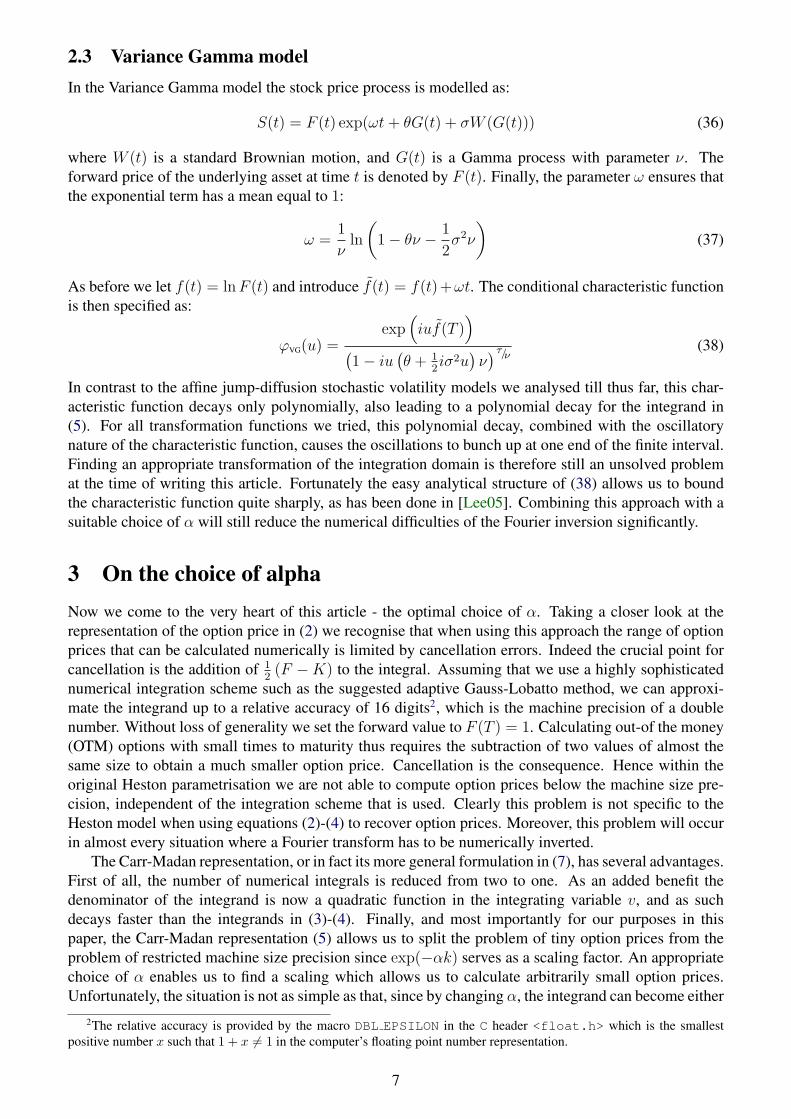
Nonetheless, choosing the right α can be very important, in particular for short maturities and/orstrikes that are away from the at-the-money level. Figure 1 shows the relative error for different valuesof α. To generate this figure we used the adaptive Gauss-Lobatto scheme on the finite interval fordifferent relative and absolute tolerance levels. It is obvious from Figure 1 that for certain contract

(A)

1e-15

1e-10

1e-05

1

100000

1e+10

1e+15

1e+20

1e+25

1e+30

100 200 300 400 500 600

Tol. 1e-2

Tol. 1e-5

Tol. 1e-8

Tol. 1e-12

(B)

1e-15

1e-10

1e-05

1

100000

1e+10

0 20 40 60 80 100 120 140 160

Tol.: 1e-2

Tol.: 1e-5

Tol.: 1e-8

Tol.: 1e-12

Figure 1: Relative pricing errors for the Heston model using the adaptive Gauss-Lobatto scheme for different absolute andrelative tolerance levels over varying values of α. Underlying: dSt = µStdt +

√VtStdWS(t) with S = F = 1 and µ = 0.

Variance: dVt = κ(θ − Vt)dt + ω√

VtdWV (t) with V0 = θ = 0.1, κ = 1, ω = 1 and ρ = −0.9. (A): τ = 1/52 and K = 2.Call value = 3.25E-126, optimal α = 541.93, (B) τ = 1/12 and K = 1.5 Call value = 1.1802E-17, optimal α = 121.24.

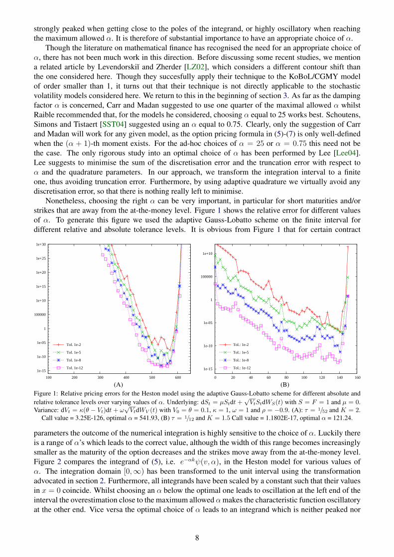
parameters the outcome of the numerical integration is highly sensitive to the choice of α. Luckily thereis a range of α’s which leads to the correct value, although the width of this range becomes increasinglysmaller as the maturity of the option decreases and the strikes move away from the at-the-money level.Figure 2 compares the integrand of (5), i.e. e−αkψ(v, α), in the Heston model for various values ofα. The integration domain [0,∞) has been transformed to the unit interval using the transformationadvocated in section 2. Furthermore, all integrands have been scaled by a constant such that their valuesin x = 0 coincide. Whilst choosing an α below the optimal one leads to oscillation at the left end of theinterval the overestimation close to the maximum allowed αmakes the characteristic function oscillatoryat the other end. Vice versa the optimal choice of α leads to an integrand which is neither peaked nor

8

oscillating at all. Since the remaining shape of the optimal characteristic function differs depending onthe parameter configuration, a standard saddle-point approximation would be too inaccurate. For thatreason we suggest to estimate the optimal α and in addition use an adaptive quadrature scheme to obtainrobust and accurate option prices. When possible, we also advocate transforming the integration domainto a finite one so that an analytical estimation of an appropriate upper limit of integration in (5) can beavoided.

(A)

-3

-2

-1

0

1

2

3

0 0.2 0.4 0.6 0.8 1

αopt = 541

αCM = 650/4

α = 400

αmax = 650

(B)

-3

-2

-1

0

1

2

3

0 0.2 0.4 0.6 0.8 1

αopt = 970

αCM = 1303/4

α = 900

αmax = 1280

Figure 2: Integrand in 5 for different values of α, where the transformation from (24) has been used. Underlying: dSt =µStdt +

√VtStdWS(t) with S = F = 1 and µ = 0. Variance: dVt = κ(θ − Vt)dt + ω

√VtdWV (t) with V0 = θ = 0.1,

κ = 1, ω = 1. (A): τ = 1/52, ρ = −0.9 and K = 2. (B) τ = 1/360, ρ = −0.2 and K = 2.4.

3.1 Minimum and maximum allowed alphaThis section examines how to determine the strip of regularity for the characteristic function, a problemwhich has already been investigated at great lengths in Andersen and Piterbarg [AP04]. Whilst Andersenand Piterbarg concentrate on the existence of ξ-th moment

µ(ζ, T ) = E[S(T )ζ

], for ζ > 1 , (39)

we want to estimate the whole strip of regularity, thus choosing ζ ∈ R such that µ(ζ, T ) < ∞. Clearlythis range will be of the form (ζ−, ζ+). Let us therefore define:

Λx = {u = x+ iy ∈ C | ζ− < −y < ζ+} . (40)

For all u ∈ Λx the existence of the characteristic function is thus guaranteed, since:

|ϕ(u)| =∣∣E[eiu ln Sτ

]∣∣ ≤ E[∣∣eiu ln Sτ

∣∣] = ϕ(iy)) . (41)

The range (α−, α+) which contains all allowed α’s clearly corresponds to (ζ− − 1, ζ+ − 1) as ψ(v, α)requires an evaluation of ϕ (v − i(α+ 1)), see (6). In the remaining subsections we give the strip ofregularity for the models considered in section 2.

3.1.1 Affine diffusion stochastic volatility model

The crucial point for explosions in the characteristic function of an affine diffusion stochastic volatilitymodel is the Ricatti equation for Bv(τ, u) given by

∂Bv

∂τ= α(u)− β(u)Bv + γB2

v . (42)

9

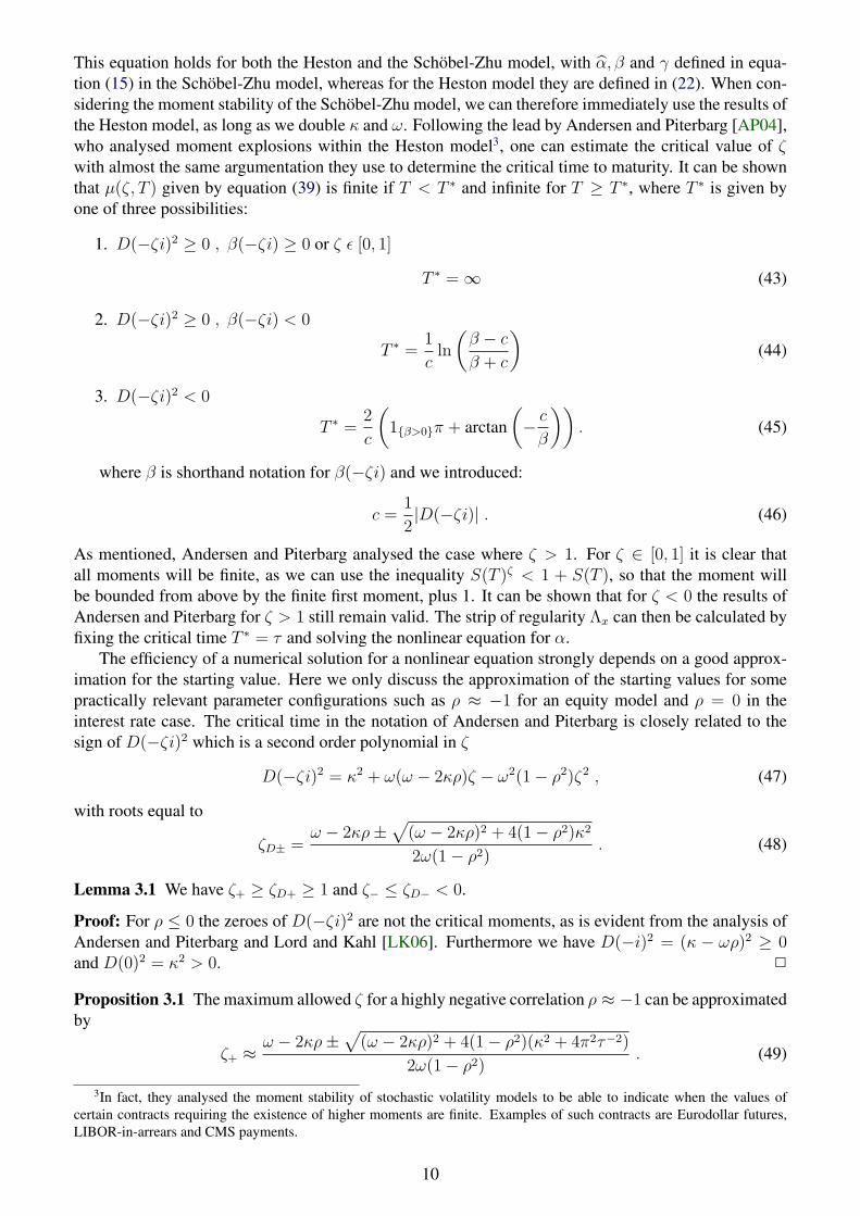
This equation holds for both the Heston and the Schobel-Zhu model, with α, β and γ defined in equa-tion (15) in the Schobel-Zhu model, whereas for the Heston model they are defined in (22). When con-sidering the moment stability of the Schobel-Zhu model, we can therefore immediately use the results ofthe Heston model, as long as we double κ and ω. Following the lead by Andersen and Piterbarg [AP04],who analysed moment explosions within the Heston model3, one can estimate the critical value of ζwith almost the same argumentation they use to determine the critical time to maturity. It can be shownthat µ(ζ, T ) given by equation (39) is finite if T < T ∗ and infinite for T ≥ T ∗, where T ∗ is given byone of three possibilities:

1. D(−ζi)2 ≥ 0 , β(−ζi) ≥ 0 or ζ ε [0, 1]

T ∗ = ∞ (43)

2. D(−ζi)2 ≥ 0 , β(−ζi) < 0

T ∗ =1

cln

(β − c

β + c

)(44)

3. D(−ζi)2 < 0

T ∗ =2

c

(1{β>0}π + arctan

(− c

β

)). (45)

where β is shorthand notation for β(−ζi) and we introduced:

c =1

2|D(−ζi)| . (46)

As mentioned, Andersen and Piterbarg analysed the case where ζ > 1. For ζ ∈ [0, 1] it is clear thatall moments will be finite, as we can use the inequality S(T )ζ < 1 + S(T ), so that the moment willbe bounded from above by the finite first moment, plus 1. It can be shown that for ζ < 0 the results ofAndersen and Piterbarg for ζ > 1 still remain valid. The strip of regularity Λx can then be calculated byfixing the critical time T ∗ = τ and solving the nonlinear equation for α.

The efficiency of a numerical solution for a nonlinear equation strongly depends on a good approx-imation for the starting value. Here we only discuss the approximation of the starting values for somepractically relevant parameter configurations such as ρ ≈ −1 for an equity model and ρ = 0 in theinterest rate case. The critical time in the notation of Andersen and Piterbarg is closely related to thesign of D(−ζi)2 which is a second order polynomial in ζ

D(−ζi)2 = κ2 + ω(ω − 2κρ)ζ − ω2(1− ρ2)ζ2 , (47)

with roots equal to

ζD± =ω − 2κρ±

√(ω − 2κρ)2 + 4(1− ρ2)κ2

2ω(1− ρ2). (48)

Lemma 3.1 We have ζ+ ≥ ζD+ ≥ 1 and ζ− ≤ ζD− < 0.

Proof: For ρ ≤ 0 the zeroes of D(−ζi)2 are not the critical moments, as is evident from the analysis ofAndersen and Piterbarg and Lord and Kahl [LK06]. Furthermore we have D(−i)2 = (κ − ωρ)2 ≥ 0and D(0)2 = κ2 > 0. 2

Proposition 3.1 The maximum allowed ζ for a highly negative correlation ρ ≈ −1 can be approximatedby

ζ+ ≈ω − 2κρ±

√(ω − 2κρ)2 + 4(1− ρ2)(κ2 + 4π2τ−2)

2ω(1− ρ2). (49)

3In fact, they analysed the moment stability of stochastic volatility models to be able to indicate when the values ofcertain contracts requiring the existence of higher moments are finite. Examples of such contracts are Eurodollar futures,LIBOR-in-arrears and CMS payments.

10

Proof: For ρ → −1, ζD+ tends to infinity so that we can approximate (45) as τ = 2π/c, leading to theanalytical solution stated in equation (49). 2

As a final remark, when we have ρ = 0, as in an interest rate setting, symmetry is introduced intothe problem: the critical time of the (ζD+ + z)th moment for z > 0 is equal to the critical time of the(ζD− − z)th moment. Furthermore ζD+ + ζD− = 1 here so that ζ+ = 1− ζ−.

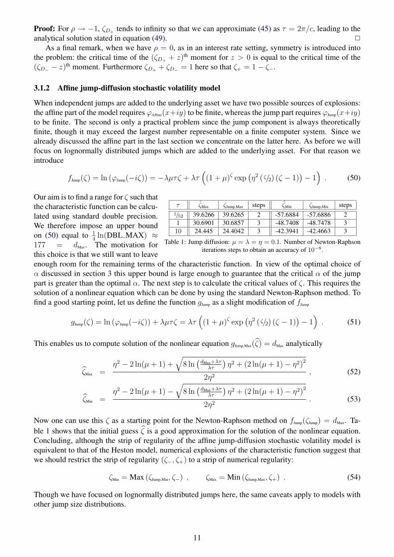
3.1.2 Affine jump-diffusion stochastic volatility model

When independent jumps are added to the underlying asset we have two possible sources of explosions:the affine part of the model requires ϕAffine(x+iy) to be finite, whereas the jump part requires ϕJump(x+iy)to be finite. The second is only a practical problem since the jump component is always theoreticallyfinite, though it may exceed the largest number representable on a finite computer system. Since wealready discussed the affine part in the last section we concentrate on the latter here. As before we willfocus on lognormally distributed jumps which are added to the underlying asset. For that reason weintroduce

fJump(ζ) = ln (ϕJump(−iζ)) = −λµτζ + λτ((1 + µ)ζ exp

(η2 ( ζ/2) (ζ − 1)

)− 1). (50)

τ ζMax ζJump,Max steps ζMin ζJump,Min steps1/52 39.6266 39.6265 2 -57.6884 -57.6886 21 30.6901 30.6857 3 -48.7408 -48.7478 310 24.445 24.4042 3 -42.3941 -42.4663 3

Table 1: Jump diffusion: µ = λ = η = 0.1. Number of Newton-Raphsoniterations steps to obtain an accuracy of 10−8.

Our aim is to find a range for ζ such thatthe characteristic function can be calcu-lated using standard double precision.We therefore impose an upper boundon (50) equal to 1

4ln(DBL MAX) ≈

177 = dMax. The motivation forthis choice is that we still want to leaveenough room for the remaining terms of the characteristic function. In view of the optimal choice ofα discussed in section 3 this upper bound is large enough to guarantee that the critical α of the jumppart is greater than the optimal α. The next step is to calculate the critical values of ζ . This requires thesolution of a nonlinear equation which can be done by using the standard Newton-Raphson method. Tofind a good starting point, let us define the function gJump as a slight modification of fJump

gJump(ζ) = ln (ϕJump(−iζ)) + λµτζ = λτ((1 + µ)ζ exp

(η2 ( ζ/2) (ζ − 1)

)− 1). (51)

This enables us to compute solution of the nonlinear equation gJump,Max(ζ) = dMax analytically

ζMax =η2 − 2 ln(µ+ 1) +

√8 ln

(dMax+λτ

λτ

)η2 + (2 ln(µ+ 1)− η2)2

2η2, (52)

ζMin =η2 − 2 ln(µ+ 1)−

√8 ln

(dMax+λτ

λτ

)η2 + (2 ln(µ+ 1)− η2)2

2η2. (53)

Now one can use this ζ as a starting point for the Newton-Raphson method on fJump(ζJump) = dMax. Ta-ble 1 shows that the initial guess ζ is a good approximation for the solution of the nonlinear equation.Concluding, although the strip of regularity of the affine jump-diffusion stochastic volatility model isequivalent to that of the Heston model, numerical explosions of the characteristic function suggest thatwe should restrict the strip of regularity (ζ−, ζ+) to a strip of numerical regularity:

ζMin = Max (ζJump,Min, ζ−) , ζMax = Min (ζJump,Max, ζ+) . (54)

Though we have focused on lognormally distributed jumps here, the same caveats apply to models withother jump size distributions.

11

3.1.3 Variance Gamma model

Due to the comparative simplicity of the characteristic function for the VG model given by equation (38),we can straightforwardly deduce the strip of regularity (ζ−, ζ+) as

ζ± = − θ

σ2±√θ2

σ4+

2

νσ2. (55)

Since the variance gamma model is fully time-homogeneous, the maximum and minimum allowed ζ ,and therefore also α, do not depend on the time to maturity, contrary to what we find in the affinejump-diffusion stochastic volatility models.

3.2 Optimal alphaBefore we embark upon our quest for the optimal α, we return to the method considered by Levendorskiıand Zherder [LZ02], which we mentioned in the beginning of this section. Their integration-along-cut (IAC) method is specifically tailored towards KoBoL/CGMY processes of order smaller than 1.For these processes it turns out that the characteristic function ϕ(u) is analytic for u ∈ C, with cuts[iζ+, i∞) and (−i∞, iζ−]. In words, this means that the characteristic function is well-defined on thewhole complex plane, apart from being discontinuous along the mentioned cuts. Instead of integratingalong (−∞−iα,∞−iα) in the complex plane to obtain the option price via equation (7), they integratealong one of the two aforementioned cuts. Unfortunately this technique is not generally applicable toany process. For example, it is shown in Lord and Kahl [LK06] that for the stochastic volatility modelswe consider here, the characteristic function has an infinite number of singularites along the imaginaryaxis. As we are seeking a method that is fully general and applicable to any model, we will thereforenot consider this method any further in this article.

The literature on option pricing has recognised the need for a good choice of α. Choosing α toosmall or too big leads to problems with either cancellation errors or highly oscillating integrands asshown in figures 1 and 2. The best α ensures that the absolute value of the integrand is as constant aspossible over the whole integration area. The oscillation of a function f : R → R on the finite interval[−1, 1] can be measured by the total variation

TV(f) =

1∫−1

∣∣∣∣∂f∂x (x)

∣∣∣∣ dx . (56)

As shown by Forster and Petras [FP91] a small total variation reduces the approximation error of theapplied numerical integration scheme. Ideally one should choose α such that the total variation of theintegrand is minimised 4

α∗ = argminα∈{αMin,αMax}

e−αk

∞∫0

∣∣∣∣ ∂∂v ψ(v, α)

ψ(0, α)

∣∣∣∣ dv . (57)

Clearly this optimization problem is of a rather theoretical nature as it has to be solved again for eachoption price and would therefore require many more function evaluations than the original problem. Arelated metric can be found by considering Figure 1, whence it is clear that in the optimal range of α’sthe derivative of the error of the numerical scheme with respect to α will roughly be equal to zero. If wechoose the squared difference between the true price and the value resulting from our numerical schemeas a relevant criterion, the first order condition for optimality becomes:

α∗ = argminα∈{αMin,αMax}

∂

∂αe−αk

∞∫0

ψ(v, α) dv . (58)

4Note that one should rescale the integrand to make the total variation comparable for different values of α.

12

where the integral on the right-hand side should be interpreted as the numerical approximation of thisintegral. A simple but highly effective idea to simplify these optimisation problems is to minimise onlythe maximal value of the integrand, which occurs in v = 0. We therefore suggest to choose α accordingto

α∗ = argminα∈{αMin,αMax}

∣∣e−αkψ (−(α+ 1)i)∣∣ . (59)

or equivalently

α∗ = argminα∈{αMin,αMax}

[−αk +

1

2ln(ψ (−(α+ 1)i)2)] =: Ψ(α, k), (60)

rendering the calculation more stable since the function ψ is not necessarily positive. Finding the optimalα thus requires to find the minimum of Ψ. The optimal α resulting from this optimisation problemwill be referred to as the payoff-dependent α, as ψ depends on the particular payoff function we areconsidering. In the following we will also consider a payoff-independent alternative:

α∗ = argminα∈{αMin,αMax}

[−αk + ln(ϕ (−(α+ 1)i))] =: Φ(α, k) , (61)

Coincidentally, this payoff-independent way of choosing α has a close link to how the optimal contouris chosen in the area of saddlepoint approximations, something we discuss in the following section.A related article by Choudhury and Whitt [CW97] considers the contour shift following from (60) toavoid numerical problems in the numerical inversion of non-probability transforms. To the best of ourknowledge this choice of α has not been picked up in the area of option pricing.

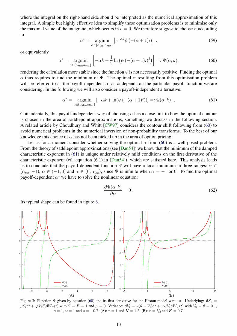
Let us for a moment consider whether solving the optimal α from (60) is a well-posed problem.From the theory of saddlepoint approximations (see [Dan54]) we know that the minimum of the dampedcharacteristic exponent in (61) is unique under relatively mild conditions on the first derivative of thecharacteristic exponent (cf. equation (6.1) in [Dan54]), which are satisfied here. This analysis leadsus to conclude that the payoff-dependent function Ψ will have a local minimum in three ranges: α ∈(αMin,−1), α ∈ (−1, 0) and α ∈ (0, αMax), since Ψ is infinite when α = −1 or 0. To find the optimalpayoff-dependent α∗ we have to solve the nonlinear equation:

∂Ψ(α, k)

∂α= 0 . (62)

Its typical shape can be found in figure 3.

(A)

-8

-6

-4

-2

0

2

4

-2 0 2 4 6 8

Ψ(α)

Ψα(α)

(B)

-8

-6

-4

-2

0

2

4

-5 0 5 10 15

Ψ(α)

Ψα(α)

Figure 3: Function Ψ given by equation (60) and its first derivative for the Heston model w.r.t. α. Underlying: dSt =µStdt +

√VtStdWS(t) with S = F = 1 and µ = 0. Variance: dVt = κ(θ − Vt)dt + ω

√VtdWV (t) with V0 = θ = 0.1,

κ = 1, ω = 1 and ρ = −0.7. (A): τ = 1 and K = 1.2. (B): τ = 1/2 and K = 0.7.

13

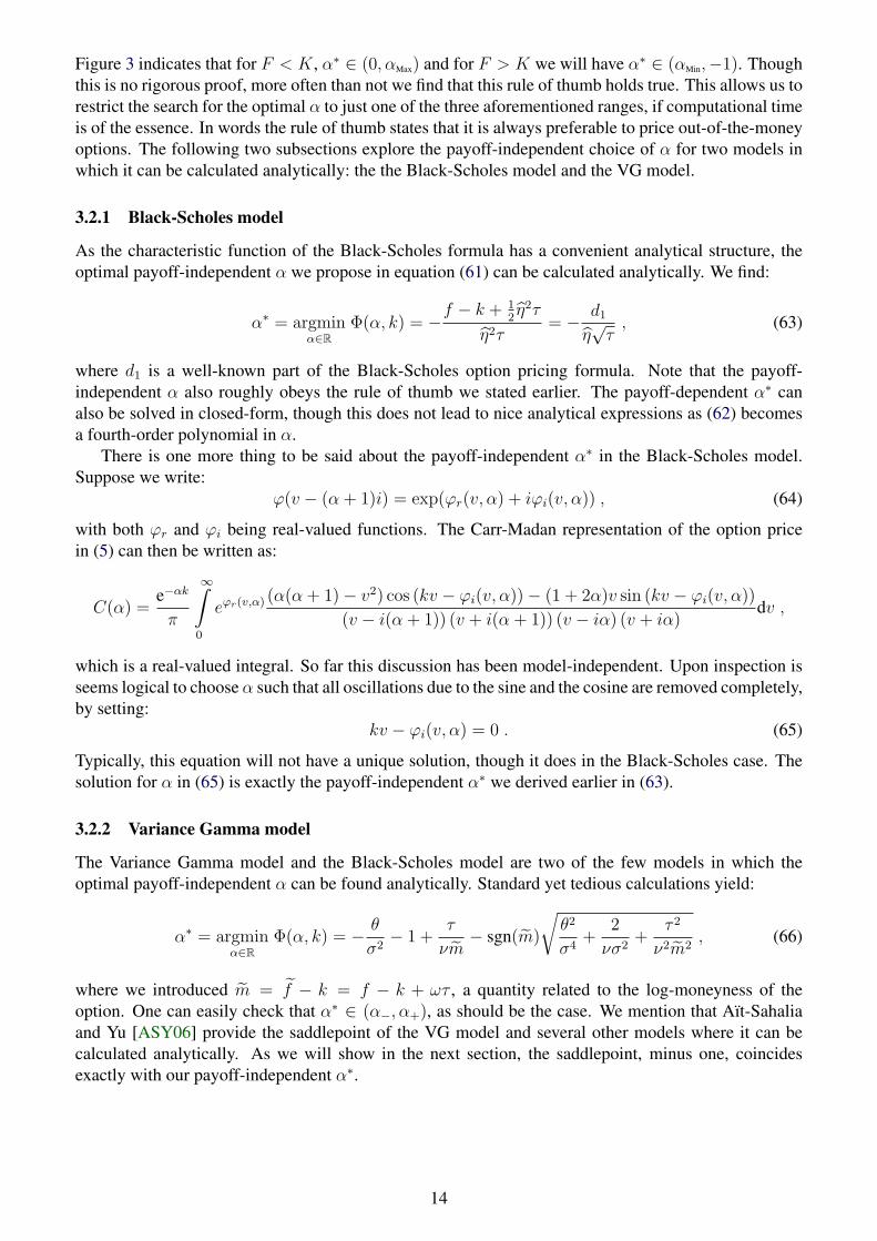
Figure 3 indicates that for F < K, α∗ ∈ (0, αMax) and for F > K we will have α∗ ∈ (αMin,−1). Thoughthis is no rigorous proof, more often than not we find that this rule of thumb holds true. This allows us torestrict the search for the optimal α to just one of the three aforementioned ranges, if computational timeis of the essence. In words the rule of thumb states that it is always preferable to price out-of-the-moneyoptions. The following two subsections explore the payoff-independent choice of α for two models inwhich it can be calculated analytically: the the Black-Scholes model and the VG model.

3.2.1 Black-Scholes model

As the characteristic function of the Black-Scholes formula has a convenient analytical structure, theoptimal payoff-independent α we propose in equation (61) can be calculated analytically. We find:

α∗ = argminα∈R

Φ(α, k) = −f − k + 1

2η2τ

η2τ= − d1

η√τ, (63)

where d1 is a well-known part of the Black-Scholes option pricing formula. Note that the payoff-independent α also roughly obeys the rule of thumb we stated earlier. The payoff-dependent α∗ canalso be solved in closed-form, though this does not lead to nice analytical expressions as (62) becomesa fourth-order polynomial in α.

There is one more thing to be said about the payoff-independent α∗ in the Black-Scholes model.Suppose we write:

ϕ(v − (α+ 1)i) = exp(ϕr(v, α) + iϕi(v, α)) , (64)

with both ϕr and ϕi being real-valued functions. The Carr-Madan representation of the option pricein (5) can then be written as:

C(α) =e−αk

π

∞∫0

eϕr(v,α) (α(α+ 1)− v2) cos (kv − ϕi(v, α))− (1 + 2α)v sin (kv − ϕi(v, α))

(v − i(α+ 1)) (v + i(α+ 1)) (v − iα) (v + iα)dv ,

which is a real-valued integral. So far this discussion has been model-independent. Upon inspection isseems logical to choose α such that all oscillations due to the sine and the cosine are removed completely,by setting:

kv − ϕi(v, α) = 0 . (65)

Typically, this equation will not have a unique solution, though it does in the Black-Scholes case. Thesolution for α in (65) is exactly the payoff-independent α∗ we derived earlier in (63).

3.2.2 Variance Gamma model

The Variance Gamma model and the Black-Scholes model are two of the few models in which theoptimal payoff-independent α can be found analytically. Standard yet tedious calculations yield:

α∗ = argminα∈R

Φ(α, k) = − θ

σ2− 1 +

τ

νm− sgn(m)

√θ2

σ4+

2

νσ2+

τ 2

ν2m2, (66)

where we introduced m = f − k = f − k + ωτ , a quantity related to the log-moneyness of theoption. One can easily check that α∗ ∈ (α−, α+), as should be the case. We mention that Aıt-Sahaliaand Yu [ASY06] provide the saddlepoint of the VG model and several other models where it can becalculated analytically. As we will show in the next section, the saddlepoint, minus one, coincidesexactly with our payoff-independent α∗.

14

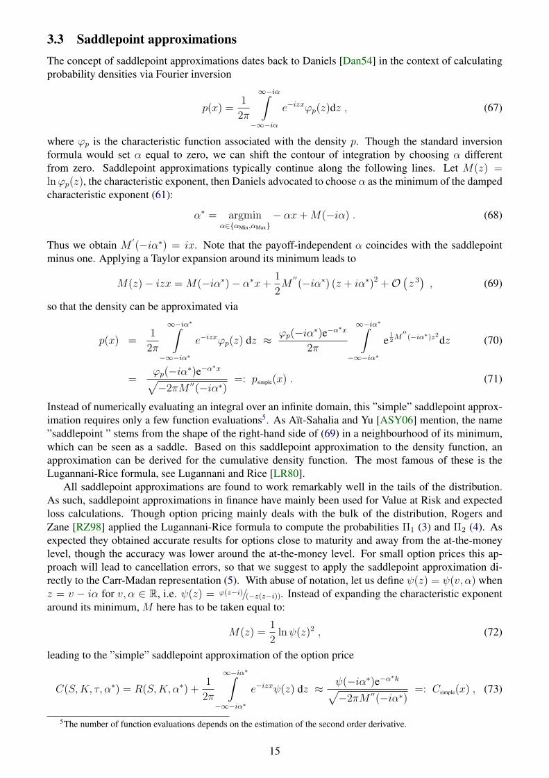
3.3 Saddlepoint approximationsThe concept of saddlepoint approximations dates back to Daniels [Dan54] in the context of calculatingprobability densities via Fourier inversion

p(x) =1

2π

∞−iα∫−∞−iα

e−izxϕp(z)dz , (67)

where ϕp is the characteristic function associated with the density p. Though the standard inversionformula would set α equal to zero, we can shift the contour of integration by choosing α differentfrom zero. Saddlepoint approximations typically continue along the following lines. Let M(z) =lnϕp(z), the characteristic exponent, then Daniels advocated to choose α as the minimum of the dampedcharacteristic exponent (61):

α∗ = argminα∈{αMin,αMax}

− αx+M(−iα) . (68)

Thus we obtain M ′(−iα∗) = ix. Note that the payoff-independent α coincides with the saddlepoint

minus one. Applying a Taylor expansion around its minimum leads to

M(z)− izx = M(−iα∗)− α∗x+1

2M

′′(−iα∗) (z + iα∗)2 +O

(z 3), (69)

so that the density can be approximated via

p(x) =1

2π

∞−iα∗∫−∞−iα∗

e−izxϕp(z) dz ≈ ϕp(−iα∗)e−α∗x

2π

∞−iα∗∫−∞−iα∗

e12M′′(−iα∗)z2

dz (70)

=ϕp(−iα∗)e−α∗x√−2πM ′′(−iα∗)

=: psimple(x) . (71)

Instead of numerically evaluating an integral over an infinite domain, this ”simple” saddlepoint approx-imation requires only a few function evaluations5. As Aıt-Sahalia and Yu [ASY06] mention, the name”saddlepoint ” stems from the shape of the right-hand side of (69) in a neighbourhood of its minimum,which can be seen as a saddle. Based on this saddlepoint approximation to the density function, anapproximation can be derived for the cumulative density function. The most famous of these is theLugannani-Rice formula, see Lugannani and Rice [LR80].

All saddlepoint approximations are found to work remarkably well in the tails of the distribution.As such, saddlepoint approximations in finance have mainly been used for Value at Risk and expectedloss calculations. Though option pricing mainly deals with the bulk of the distribution, Rogers andZane [RZ98] applied the Lugannani-Rice formula to compute the probabilities Π1 (3) and Π2 (4). Asexpected they obtained accurate results for options close to maturity and away from the at-the-moneylevel, though the accuracy was lower around the at-the-money level. For small option prices this ap-proach will lead to cancellation errors, so that we suggest to apply the saddlepoint approximation di-rectly to the Carr-Madan representation (5). With abuse of notation, let us define ψ(z) = ψ(v, α) whenz = v − iα for v, α ∈ R, i.e. ψ(z) = ϕ(z−i)/(−z(z−i)). Instead of expanding the characteristic exponentaround its minimum, M here has to be taken equal to:

M(z) =1

2lnψ(z)2 , (72)

leading to the ”simple” saddlepoint approximation of the option price

C(S,K, τ, α∗) = R(S,K, α∗) +1

2π

∞−iα∗∫−∞−iα∗

e−izxψ(z) dz ≈ ψ(−iα∗)e−α∗k√−2πM ′′(−iα∗)

=: Csimple(x) , (73)

5The number of function evaluations depends on the estimation of the second order derivative.

15

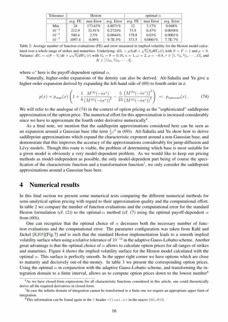
Tolerance Heston optimal-αavg. FE max Error avg. Error avg. FE max Error avg. Error

Min. 24 173.63% 4.8071% 12 3.17% 0.048%10−3 212.9 32.91% 0.2724% 73.9 0.47% 0.0038%10−5 540.4 2.5% 0.0044% 179.8 0.03% 0.0001%10−7 1097.4 0.09% 9.7E-5% 373.5 0.0001% 7.7E-7%

Table 2: Average number of function evaluations (FE) and error measured in implied volatility for the Heston model calcu-lated over a whole range of strikes and maturities. Underlying: dSt = µStdt +

√VtStdWS(t) with S = F = 1 and µ = 0.

Variance: dVt = κ(θ − Vt)dt + ω√

VtdWV (t) with V0 = θ = 0.16, κ = 1, ω = 2, ρ = −0.8, τ ∈ [1, 5/4, 6/4, · · · , 15], andK ∈ [1/10, 2/10, · · · , 4].

where α∗ here is the payoff-dependent optimal α.Naturally, higher-order expansions of the density can also be derived. Aıt-Sahalia and Yu give a

higher-order expansion derived by expanding the left-hand side of (69) to fourth order in z:

p(x) = psimple(x)

(1 +

1

8

M (4)(−iα∗)(M (2)(−iα∗))2 −

5

24

(M (3)(−iα∗)

)2(M (2)(−iα∗))3

)=: psophisticated(x) . (74)

We will refer to the analogue of (74) in the context of option pricing as the ”sophisticated” saddlepointapproximation of the option price. The numerical effort for this approximation is increased considerablysince we have to approximate the fourth order derivative numerically6.

As a final note, we mention that the saddlepoint approximations considered here can be seen asan expansion around a Gaussian base (the term 1

2z2 in (69)). Aıt-Sahalia and Yu show how to derive

saddlepoint approximations which expand the characteristic exponent around a non-Gaussian base, anddemonstrate that this improves the accuracy of the approximations considerably for jump-diffusion andLevy models. Though this route is viable, the problem of determining which base is most suitable fora given model is obviously a very model-dependent problem. As we would like to keep our pricingmethods as model-independent as possible, the only model-dependent part being of course the speci-fication of the characteristic function and a transformation function7, we only consider the saddlepointapproximations around a Gaussian base here.

4 Numerical resultsIn this final section we present some numerical tests comparing the different numerical methods forsemi-analytical option pricing with regard to their approximation quality and the computational effort.In table 2 we compare the number of function evaluations and the computational error for the standardHeston formulation (cf. (2)) to the optimal-α method (cf. (7) using the optimal payoff-dependent αfrom (60)).

One can recognize that the optimal choice of α decreases both the necessary number of func-tion evaluations and the computational error. The parameter configuration was taken from Kahl andJackel [KJ05][Fig.7] and is such that the standard Heston implementation leads to a smooth impliedvolatility surface when using a relative tolerance of 10−12 in the adaptive Gauss-Lobatto scheme. Anothergreat advantage is that the optimal choice of α allows to calculate option prices for all ranges of strikesand maturities. Figure 4 shows the implied volatility surface for the Heston model calculated with theoptimal α. This surface is perfectly smooth. In the upper right corner we have options which are closeto maturity and decisively out-of-the-money. In table 3 we present the corresponding option prices.Using the optimal α in conjunction with the adaptive Gauss-Lobatto scheme, and transforming the in-tegration domain to a finite interval, allows us to compute option prices down to the lowest number8

6As we have closed-form expressions for all characteristic functions considered in this article, one could theoreticallyderive all the required derivatives in closed-form.

7In case the infinite domain of integration cannot be transformed to a finite one we require an appropriate upper limit ofintegration.

8This information can be found again in the C header <float.h> in the macro DBL MIN.

16

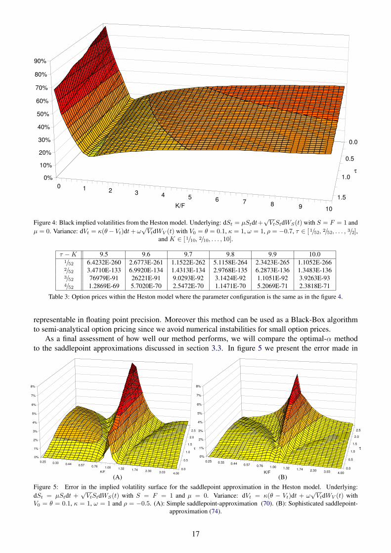
Figure 4: Black implied volatilities from the Heston model. Underlying: dSt = µStdt+√

VtStdWS(t) with S = F = 1 andµ = 0. Variance: dVt = κ(θ− Vt)dt + ω

√VtdWV (t) with V0 = θ = 0.1, κ = 1, ω = 1, ρ = −0.7, τ ∈ [1/52, 2/52, . . . , 3/2],

and K ∈ [1/10, 2/10, . . . , 10].

τ −K 9.5 9.6 9.7 9.8 9.9 10.01/52 6.4232E-260 2.6773E-261 1.1522E-262 5.1158E-264 2.3423E-265 1.1052E-2662/52 3.4710E-133 6.9920E-134 1.4313E-134 2.9768E-135 6.2873E-136 1.3483E-1363/52 76979E-91 26221E-91 9.0293E-92 3.1424E-92 1.1051E-92 3.9263E-934/52 1.2869E-69 5.7020E-70 2.5472E-70 1.1471E-70 5.2069E-71 2.3818E-71

Table 3: Option prices within the Heston model where the parameter configuration is the same as in the figure 4.

representable in floating point precision. Moreover this method can be used as a Black-Box algorithmto semi-analytical option pricing since we avoid numerical instabilities for small option prices.

As a final assessment of how well our method performs, we will compare the optimal-α methodto the saddlepoint approximations discussed in section 3.3. In figure 5 we present the error made in

(A) (B)Figure 5: Error in the implied volatility surface for the saddlepoint approximation in the Heston model. Underlying:dSt = µStdt +

√VtStdWS(t) with S = F = 1 and µ = 0. Variance: dVt = κ(θ − Vt)dt + ω

√VtdWV (t) with

V0 = θ = 0.1, κ = 1, ω = 1 and ρ = −0.5. (A): Simple saddlepoint-approximation (70). (B): Sophisticated saddlepoint-approximation (74).

17

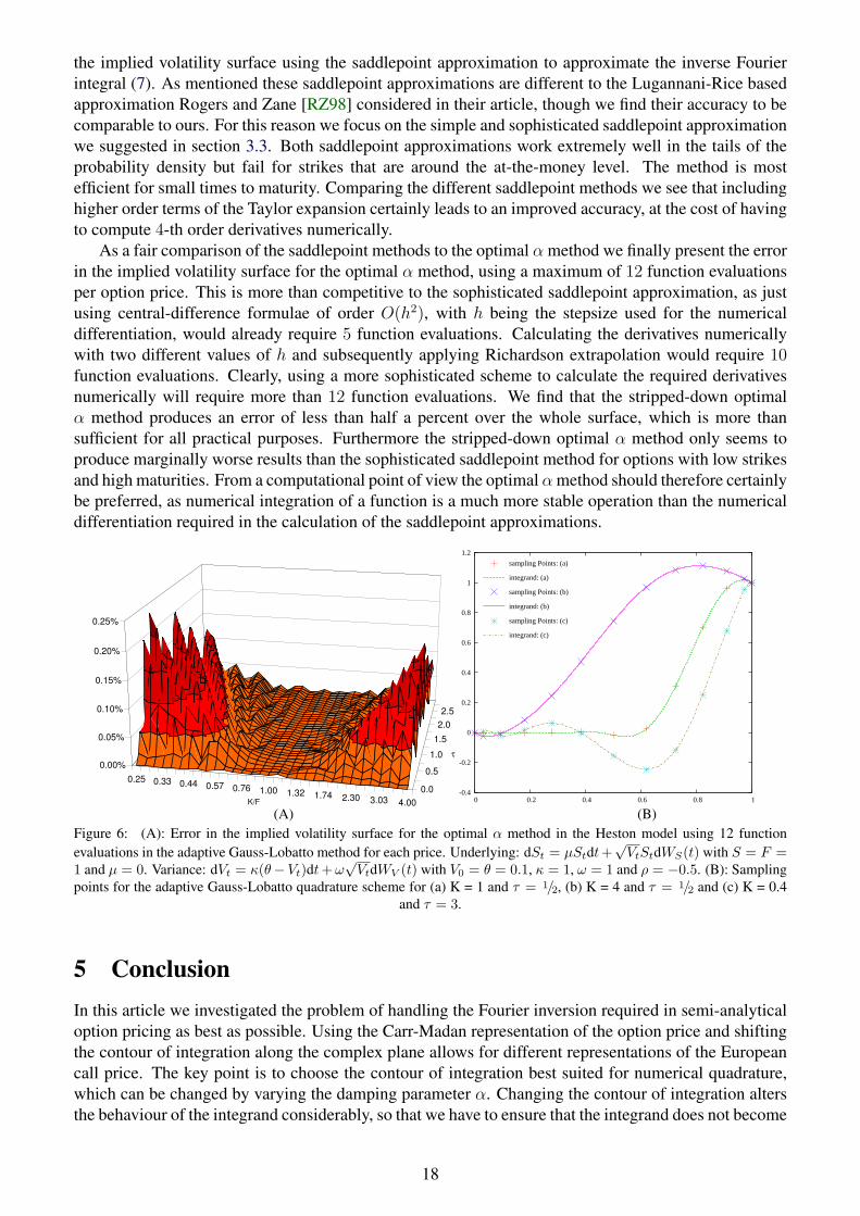
the implied volatility surface using the saddlepoint approximation to approximate the inverse Fourierintegral (7). As mentioned these saddlepoint approximations are different to the Lugannani-Rice basedapproximation Rogers and Zane [RZ98] considered in their article, though we find their accuracy to becomparable to ours. For this reason we focus on the simple and sophisticated saddlepoint approximationwe suggested in section 3.3. Both saddlepoint approximations work extremely well in the tails of theprobability density but fail for strikes that are around the at-the-money level. The method is mostefficient for small times to maturity. Comparing the different saddlepoint methods we see that includinghigher order terms of the Taylor expansion certainly leads to an improved accuracy, at the cost of havingto compute 4-th order derivatives numerically.

As a fair comparison of the saddlepoint methods to the optimal α method we finally present the errorin the implied volatility surface for the optimal α method, using a maximum of 12 function evaluationsper option price. This is more than competitive to the sophisticated saddlepoint approximation, as justusing central-difference formulae of order O(h2), with h being the stepsize used for the numericaldifferentiation, would already require 5 function evaluations. Calculating the derivatives numericallywith two different values of h and subsequently applying Richardson extrapolation would require 10function evaluations. Clearly, using a more sophisticated scheme to calculate the required derivativesnumerically will require more than 12 function evaluations. We find that the stripped-down optimalα method produces an error of less than half a percent over the whole surface, which is more thansufficient for all practical purposes. Furthermore the stripped-down optimal α method only seems toproduce marginally worse results than the sophisticated saddlepoint method for options with low strikesand high maturities. From a computational point of view the optimal αmethod should therefore certainlybe preferred, as numerical integration of a function is a much more stable operation than the numericaldifferentiation required in the calculation of the saddlepoint approximations.

(A) (B)

-0.4

-0.2

0

0.2

0.4

0.6

0.8

1

1.2

0 0.2 0.4 0.6 0.8 1

sampling Points: (a)

integrand: (a)

sampling Points: (b)

integrand: (b)

sampling Points: (c)

integrand: (c)

Figure 6: (A): Error in the implied volatility surface for the optimal α method in the Heston model using 12 functionevaluations in the adaptive Gauss-Lobatto method for each price. Underlying: dSt = µStdt+

√VtStdWS(t) with S = F =

1 and µ = 0. Variance: dVt = κ(θ−Vt)dt + ω√

VtdWV (t) with V0 = θ = 0.1, κ = 1, ω = 1 and ρ = −0.5. (B): Samplingpoints for the adaptive Gauss-Lobatto quadrature scheme for (a) K = 1 and τ = 1/2, (b) K = 4 and τ = 1/2 and (c) K = 0.4

and τ = 3.

5 ConclusionIn this article we investigated the problem of handling the Fourier inversion required in semi-analyticaloption pricing as best as possible. Using the Carr-Madan representation of the option price and shiftingthe contour of integration along the complex plane allows for different representations of the Europeancall price. The key point is to choose the contour of integration best suited for numerical quadrature,which can be changed by varying the damping parameter α. Changing the contour of integration altersthe behaviour of the integrand considerably, so that we have to ensure that the integrand does not become

18

too peaked or too oscillatory. Furthermore, cancellation errors also have to be avoided at all cost. Bytransforming the integration domain as discussed in section 2, as well as choosing the optimal α as insection 3, we obtain a call price formula which allows for a robust implementation enabling us to priceoptions down to machine size precision. The optimal choice of the damping parameter α is the onlyway to overcome any numerical instabilities and guarantee accurate results.

A ProofsIn this section we present the missing proofs. Proof: [Prop. 2.1] One can successively deduce that

limu→∞

β(u)

u= −2iρω =: i · β∞

limu→∞

D(u)

u= 2ω

√1− ρ2 =: D∞

limu→∞

G(u) = const .

Using the limiting behaviour of D we can directly deduce that

limu→∞

Aσ(u) = 0 ,

as well aslim

u→∞Bσ(u) = 0 ,

which finally leads to

limu→∞

A(u)

u=

1

4(β∞ −D∞)τ ,

limu→∞

Bv(u)

u=

β∞ −D∞

2γ.

Combining all result we obtainC∞ = D∞

(τ + V0/ω

2)/4 .

which completes the proof. 2

References[AA02] L.B.G. Andersen and J. Andreasen. Volatile volatilities. Risk, 15(12):163–168, 2002.

[AP04] L. Andersen and V. Piterbarg. Moment Explosions in Stochastic Volatilty Models. Technicalreport, Bank of America, 2004. ssrn.com/abstract=559481.

[ASY06] Y. Aıt-Sahalia and Jialin. Yu. Saddlepoint Approximations for Continuous-Time MarkovProcesses. Working paper, 2006. http://www.http://www.princeton.edu/∼yacine/saddlepoint.pdf.

[Bat96] D.S. Bates. Jumps and Stochastic Volatility: Exchange Rate Processes Implicit in DeutscheMark Options. The Review of Financial Studies, 9(1):69–107, 1996.

[CM99] P. Carr and D. Madan. Option valuation using the Fast Fourier Transform. Journal of Com-putational Finance, 2(4):61–73, 1999.

19

[CS05] P. Cheng and O. Scailett. Linear-quadratic jump-diffusion modelling with application tostochastic volatility. Working paper, Credit Suisse, FAME and HEC Geneve, 2005.

[CW97] G.L. Choudhury and W. Whitt. Probabilistic scaling for the numerical inversion of non-probability transforms. INFORMS J. Computing, 9:175–184, 1997.

[DA68] H. Dubner and J. Abate. Numerical inversion of Laplace transforms by relating them to thefinite Fourier cosine transform. Journal of the ACM, 15(1):115–123, 1968.

[Dan54] H.E. Daniels. Saddlepoint Approximations in Statistics. The Annals of Mathematical Statis-tics, 25(4):631–650, 1954.

[FP91] K.-J. Forster and K. Petras. Error estimates in Gaussian quadrature for functions of boundedvariations. SIAM Journal of Numerical Analysis, 28(3):880–889, 1991.

[Gas04] R. Gaspar. General quadratic term structures of bond, futures and forward prices. SSE/EFIWorking paper Series in Economics and Finance, (559), 2004.

[GG00] W. Gander and W. Gautschi. Adaptive Quadrature — Revisited. BIT, 40(1):84–101, March 2000. CS technical report: ftp.inf.ethz.ch/pub/publications/tech-reports/3xx/306.ps.gz.

[GP51] J. Gil-Pelaez. Note on the inversion theorem. Biometrika, 37:481–482, 1951.

[Gur48] J. Gurland. Inversion formulae for the distribution of ratios. Annals of Mathematical Statis-tics, 19:228–237, 1948.

[Hes93] S. L. Heston. A closed-form solution for options with stochastic volatility with applicationsto bond and currency options. The Review of Financial Studies, 6:327–343, 1993.

[KJ05] C. Kahl and P. Jackel. Not-so-complex logarithms in the Heston model. Wilmott, September,2005. http://www.math.uni-wuppertal.de/∼kahl/publications.html.

[Lee04] R. Lee. The Moment Formula for Implied Volatility at Extreme Strikes. Mathematical Fi-nance, 14:469–480, 2004.

[Lee05] R. Lee. Option Pricing by Transform Methods: Extensions, Unification, and Error Control.Journal of Computational Finance, 7(3):51–86, 2005.

[Lev25] P. Levy. Calcul des probabilites. Gauthier-Villars, Paris, 1925.

[Lew01] A. Lewis. A Simple Option Formula for General Jump-Diffusion and Other Exponential LevyProcesses. 2001. http://ssrn.com/abstract=282110.

[LK06] R. Lord and C. Kahl. Why the rotation count algorithm works. Working pa-per, 2006. http://www.math.uni-wuppertal.de/∼kahl/publications/WhyTheRotationCountAlgorithmWorks.pdf.

[LR80] R. Lugannani and S. Rice. Saddlepoint approximation for the distribution of the sum ofindependent random variables. Advanceds in Applied Probabilit, 12:475–490, 1980.

[Luk70] E. Lukacs. Characteristic functions. Griffin, London, 1970.

[LZ02] S. Levendorskiı and V.M. Zherder. Fast option pricing under regular Levy processes of ex-ponential type. working paper, University of Texas at Austin and Rostov State University ofEconomics, 2002.

20

[Rai00] S. Raible. Levy Processes in Finance: Theory, Numerics and Empirical Facts. PhD thesis,Albert-Ludwigs-Universitat Freiburg, Germany, 2000.

[RZ98] L.C.G. Rogers and O. Zane. Saddlepoint approximations to option pricing. The annals ofapplied probability, 9(2), 1998.

[SS91] E. Stein and J. Stein. Stock-Price Distributions with Stochastic Volatility - An AnalyticApproach. Review of Financial Studies, 4:727–752, 1991.

[SST04] W. Schoutens, E. Simons, and J. Tistaert. A perfect calibration! Now what? Wilmott Maga-zine, March 2004.

[SZ99] R. Schobel and J. Zhu. Stochastic Volatility with an Ornstein-Uhlenbeck Process: An Exten-sion. European Finance Review, 3:23–46, 1999.

21