Define Universe and Give Two Examples 565 A Brief Guide to
23
Define Universe and Give Two Examples A Brief Guide to Appendix F Appendix F appears in a popular-level book intended to illustrate, among other things, the depth and fullness of science and the devotion of most scientists to the discovery of universal truth. Because this appendix includes a summary from scratch of elementary statistical mechanics, it is somewhat lengthy and tedious to read, and unnecessary to read completely if one is already familiar with the topic. However, some of the early material is vital to later, original material be- cause the method used in deriving novel results is illustrated and justified in deriv- ing the well-known canonical distribution. This method is called the Maxent method, short for maximization of system information entropy subject to constraints charac- teristic of a system type, or even of a particular system. Maxent provides a most probable distribution characterizing each type of system. It surely applies to equi- librium systems and it is supposed that it also applies to stationary systems that are not in equilibrium. It may well even apply to quasi-stationary systems. In every case, the resulting distribution corresponds to maximum system information (Boltz- mann) entropy and, therefore, presumably to the most probable system state. Maxent thus appears to provide a powerful capability for characterizing nonequilibrium sys- tems and processes. Theories like the present one will provide tests of the principle. In Section 2 the Boltzmann entropy and Boltzmann’s H theorem are de- scribed (old news). Section 3 contains a summary of results of the Maxent method for various system types. Sections 4 and 5 describe derivations of the microcanonical and canonical distributions. None of these results are original but Section 5 is useful in introducing and illustrating the Maxent method. Original results start in Section 6 and continue through Section 8 based on results derived in Section 6. The core physics of the paper are thus described in Section 6 in which the velocity distribution of dilute (perfect) gas molecules is derived for a gas containing a stationary, nonuniform, temperature field. As in Sec- tion 5, the problem is posed and solved. Novelty of Section 6 lies in the fact that the local velocity distribution of molecules in a closed, stationary-but-nonequilibrium system applies at specified temperature and at specified temperature gradient. The two key results of Section 6 are the nonequilibrium velocity distribu- tion in a temperature gradient, given by Equation [F4], and a balancing counterflow velocity required to conserve mass or number of molecules, given by Equation [F7a]. These are the core physics, the critical results, used in the remainder of the paper. In Section 7 the standard problems of heat, momentum, and mass transfer are addressed. While the problems are standard, the results are not. In the heat transfer result two coupled terms appear, one proportional to temperature gradient and one to concentration gradient. This result predicts the Dufour or diffusion thermo effect. This effect has previously been invisible in any treatment of such simplicity. One virtue of the method is therefore that it faithfully represents complex processes by means of a simple theory. And, when compared to “rigorous” or Chapman-Enskog theory, simplicity is a highly desired quality because some results of the Chapman- Enskog theory are very complex and appear to be fundamentally incorrect, a prop- erty previously lost in their complexity.
Transcript of Define Universe and Give Two Examples 565 A Brief Guide to
Define Universe and Give Two Examples 565
A Brief Guide to Appendix FAppendix F appears in a popular-level book intended to illustrate, among
other things, the depth and fullness of science and the devotion of most scientists tothe discovery of universal truth. Because this appendix includes a summary fromscratch of elementary statistical mechanics, it is somewhat lengthy and tedious toread, and unnecessary to read completely if one is already familiar with the topic.
However, some of the early material is vital to later, original material be-cause the method used in deriving novel results is illustrated and justified in deriv-ing the well-known canonical distribution. This method is called the Maxent method,short for maximization of system information entropy subject to constraints charac-teristic of a system type, or even of a particular system. Maxent provides a mostprobable distribution characterizing each type of system. It surely applies to equi-librium systems and it is supposed that it also applies to stationary systems that arenot in equilibrium. It may well even apply to quasi-stationary systems. In everycase, the resulting distribution corresponds to maximum system information (Boltz-mann) entropy and, therefore, presumably to the most probable system state. Maxentthus appears to provide a powerful capability for characterizing nonequilibrium sys-tems and processes. Theories like the present one will provide tests of the principle.
In Section 2 the Boltzmann entropy and Boltzmann’s H theorem are de-scribed (old news). Section 3 contains a summary of results of the Maxent method forvarious system types. Sections 4 and 5 describe derivations of the microcanonicaland canonical distributions. None of these results are original but Section 5 is usefulin introducing and illustrating the Maxent method.
Original results start in Section 6 and continue through Section 8 based onresults derived in Section 6. The core physics of the paper are thus described inSection 6 in which the velocity distribution of dilute (perfect) gas molecules isderived for a gas containing a stationary, nonuniform, temperature field. As in Sec-tion 5, the problem is posed and solved. Novelty of Section 6 lies in the fact that thelocal velocity distribution of molecules in a closed, stationary-but-nonequilibriumsystem applies at specified temperature and at specified temperature gradient.
The two key results of Section 6 are the nonequilibrium velocity distribu-tion in a temperature gradient, given by Equation [F4], and a balancing counterflowvelocity required to conserve mass or number of molecules, given by Equation [F7a].These are the core physics, the critical results, used in the remainder of the paper.
In Section 7 the standard problems of heat, momentum, and mass transferare addressed. While the problems are standard, the results are not. In the heattransfer result two coupled terms appear, one proportional to temperature gradientand one to concentration gradient. This result predicts the Dufour or diffusion thermoeffect. This effect has previously been invisible in any treatment of such simplicity.One virtue of the method is therefore that it faithfully represents complex processesby means of a simple theory. And, when compared to “rigorous” or Chapman-Enskogtheory, simplicity is a highly desired quality because some results of the Chapman-Enskog theory are very complex and appear to be fundamentally incorrect, a prop-erty previously lost in their complexity.

566 Appendix F
Section 7 also contains results for momentum and mass transfer. The formerresult, Equation [F9], does not differ fundamentally from previous results but thelatter does. In Equations [F11] we obtain a pair of coupled transport equations, onefor each component of a binary mixture, which contain all coefficients explicitlydefined. This result is new, with previous results having been misdirected by as-sumptions dating back to the origins of Chapman-Enskog theory. Such assumptionsand much complexity are avoided here by using dependent variables ζϕ(z), n(z), andT(z), with ζϕ the local number fraction of species-ϕ molecules, n(z) = P / kT the localnumber concentration of all molecules, and T(z) the local temperature. Then, localconcentration of species-ϕ molecules, n(z) ζϕ(z), contains its complete temperaturedependence in n(z) and its complete concentration dependence in ζϕ(z). Complexityand confusion in writing gradients are thus removed, avoiding past errors.
In Equations [F11] both molecular and thermal diffusion emerge, the firstdue to a concentration gradient and the second due to a temperature gradient. Againwe find the simple theory producing a subtle effect, in this case the Soret or thermaldiffusion effect, invisible in other theories of comparable simplicity. And again thecoefficients for coupled molecular diffusion and thermal diffusion are explicitlydefined. These results replace long-standing, widely-used standards that are 50years old, but incorrect in that coefficients are either incorrectly or not defined.
Diffusion and thermal diffusion are the worst-predicted processes of therigorous theory. Errors in past analyses have been corrected here by (1) using quan-tities n(z), ζϕ(z), and T(z) as variables in the transport equations, (2) including tran-sient and stationary counterflow velocity necessary for correct characterization ofall transport, and (3) basing the theory on an apparently reliable foundation: maxi-mization of system information entropy with required physical constraints. Indeed,this last feature may be regarded as the fundamental cause of all transport and manyother nonequilibrium phenomena and equilibrium properties.
Finally the thermophoresis and diffusiophoresis processes are addressed,the former being migration of individual particles in a temperature gradient in asuspending gas and the latter their migration in a concentration gradient in the gas.
To predict phoretic migrations, the molecular velocity distribution [F4]must be adapted to apply to individual, isolated particles (or molecules) instead ofnumerous, distributed gas molecules. The adaptation is simple and intuitive andprovides correct results, exact within 50 % at worst and maybe outright exact. Whilemolecules are driven by thermal diffusion in the direction of the temperature gradi-ent, suspended particles are driven in the opposite direction. For particles suspendedin a gas mixture, a stationary migration of particles is proportional to concentrationgradient of a gas species thus predicting the diffusiophoretic effect. One final result,Equation [F20], gives migration velocity of a suspended particle due to both a tem-perature and a concentration gradient, a combined phoretic velocity.
That all these generally-applicable results, previously underived with alltheir coefficients explicitly defined, are derived directly from a simple molecularvelocity distribution is rather remarkable and, if they agree with observation, theywill serve to support the validity of the nonequilibrium velocity distribution inparticular and the Maxent method in general.

Define Universe and Give Two Examples 567
567
Appendix F
Thermodynamics, Statistical Mechanics, and Kinetic Theory
1. Thermodynamic Laws, Systems, and Entropy
In Chapter 10 we described the first law of classical or macroscopic thermo-dynamics as the conservation of energy in a system in which heat Q is recognized asa form of energy. In its most general form the first law of thermodynamics is written
Q = ∆E + min× E
in – m
out× E
out – W,
where Q is heat addition to the system, ∆E is energy increase of the system, min and
mout
are masses added to and extracted from the system, Ein and E
out are the energy
contents per unit mass of the added and extracted masses, and W is work energyextracted from the thermodynamic system.1 This form of the law applies for an opensystem in which mass, heat, energy, and work may all be exchanged. For a closedsystem, no mass exchange occurs and the law applies but with m
in = m
out = 0. For an
isolated system, no mass or heat or energy or work exchange occurs. However, energymay be internally converted into heat for which process ∆E = ∆E
i + Q
i = 0.
We also mentioned in Chapter 10 that Rudolf Clausius et al discovered anequilibrium-state property of a system that he eventually named entropy. Change inentropy of a system due to heat Q transferred to the system is ∆S = Q/T + I, where Tis the absolute temperature of the heat (source) and I is the irreversibility of theprocess due to, say, friction or electrical resistance or …. In ideal processes I = 0 and∆S = Q/T, the only classical-thermodynamics type of process in which entropychange is exactly defined. For a real process wherein I ≥ 0 we write ∆S ≥ Q/T.
Clausius stated the second law of thermodynamics as follows: “Nospontaneous process in an isolated system causes system entropy to decrease.” Thislaw has been stated in other forms and we soon consider a famous one due to L. Boltzmann.
The universe exemplifies an isolated system, i.e., no transfer of energy, work,heat, or matter to or from the system. In such systems, evolution toward maximumentropy proceeds by internal processes by which, in the vicissitudes of spontaneousenergy fluctuations even in the vacuum, some energy is inexorably converted to heat,a form of energy from which there is never a full or reversible return to any other. Thisuniversal, at-least-partially mono-directional process is relentless in its effect: isolatedsystems ever evolve toward their only possible stationary or equilibrium state, referredto as a “heat-death,” in which system entropy is maximized and all system energy isunusable heat.2 Clausius’ (and Boltzmann’s) statement conveys the relentless natureof entropy production in spontaneous generation and exchange of heat.
Entropy extended the scope of thermodynamics, especially beginning inthe 1870s when Austrian physicist Ludwig Boltzmann (1844-1906) began developingpowerful statistical mechanics thereby extending James Clerk Maxwell’s introductionof statistical methods to physics in his 1859 and 1864 kinetic theories of gases.
Appendix F from Define Universe and Give Two Examples,Barton E. Dahneke, BDS Publications, Palmyra, NY, 2006.(http://defineuniverse.com) Revised 12 December 2007.
568 Appendix F
Traditional classical thermodynamics considers macroscopic characterization ofsystems by their bulk properties, such as system volume V, pressure P, and energy E.But in statistical mechanics we seek deeper understanding at a more fundamental,microscopic level in characterization of systems by atomic (or even subatomic)properties, such as atom velocities. Moreover, we seek a methodology in statisticalmechanics useful for small numbers of atoms and for nonequilibrium systems,possibilities not contemplated in traditional, macroscopic thermodynamics.
2. Entropy in Statistical Mechanics
Throughout Boltzmann’s life most scientists held a preconception againstthe atomic theory of matter (illustrated by J. J. Waterston’s experience described inAppendix A). Continuum theories of matter and energy were favored as superior toatomic theories. Moreover, since Newton’s mechanics are fully reversible in time, i.e.,any solution for forward flowing (positive) time applies equally for backward flowing(negative) time, physicists objected to the concept of a thermodynamic property, ent-ropy, that only increases in time until it reaches a stationary, maximum value. Howcould such a process be consistent with the fully reversible mechanics of the atomsinvolved? To justify the atomic-molecular theory of matter and the existence of anentropy-like property in time-reversible mechanics, Boltzmann sought and discovereda gas property he called H that continually decreases in time until it reaches a stationary,minimum value. Boltzmann’s H-theorem states that the time-rate-of-change of H isless than or equal to zero, i.e., dH/dt ≤ 0, with H defined by3 H = Σ
j p
j log
e(p
j). In this
sum, index j indicates a system state. The sum includes all states accessible to thesystem, corresponding to many microscopic configurations or microscopic states ormicrostates consistent with its bulk-properties state (i.e., everything we know aboutthe system). Each such microstate is assumed to be equally probable. The probabilityp
j that the system is in its jth discrete microstate is regarded as equal to the fraction of
an ensemble – a huge number of (imaginary) identical replications of a prototypesystem – in microstate j or the fraction of time the prototype system is in microstate j.
In quantum statistical mechanics all possible exchanges of identical atomsare counted as a single configuration (page 573), such exchanges being conceptuallybeyond any capability to detect. In addition, when system energy does not vary withposition of an atom in system volume V, many geometric configurations form differentbut bulk-property-equivalent states. The number of possible microstates of a systemis usually much larger than the number of atoms in the system.4
By its above definition and because probability pj must satisfy 0 ≤ p
j ≤ 1
and pj log
e(p
j) = 0 when p
j is zero or one and is otherwise negative, H is always
negative. Boltzmann’s H and entropy S for a dilute (or perfect) gas are related by
S = – k H = – k Σj p
j log
e(p
j) ≥ 0,
with k the Boltzmann constant. Boltzmann’s version of the second law, derived fromhis reversible-mechanics analysis of the evolving state of perfect-gas atoms, is thatisolated-system entropy only increases until it reaches a maximum value, i.e.,

Define Universe and Give Two Examples 569
dS/dt ≥ 0.
In 1902, American engineer-physicist Josiah Willard Gibbs (1839-1903)entered the statistical-mechanics story.5 He introduced the powerful concept of theensemble as a superior foundation of statistical mechanics (see endnote 11 of Chapter2) and utilized it to correct and extend Boltzmann’s results. While Boltzmann ignoredatomic interactions, Gibbs included them. Thus, Boltzmann’s results apply only fora perfect gas while Gibbs’ sometimes identical expressions, such as the one for entropyof a system, are derived from the superior conceptual basis that allows their applicationto real gases, liquids, and solids in which strong molecular interactions occur.6
To illustrate the nature of entropy and the value of Gibbs’ approach, considera closed thermodynamic system containing a solution in which a crystal (with strongatomic bonding) is forming. In a closed system, heat and energy but not matter maytransfer into or out of the system.1 A crystal represents a highly ordered state with thecrystal atoms purified and fixed in a regular structure. Before crystallization, soluteatoms are neither purified nor fixed (distinguishable) but are mixed and randomlydrifting about in the solution. When crystal growth is slow and system temperatureremains nearly fixed, the crystallization is essentially reversible. Nevertheless, systementropy decreases in such spontaneous crystallization, a claim justified in endnote 7.
What happened? Isn’t entropy supposed to increase in spontaneousprocesses? Have we encountered an enigma? A reader might say “We were led tobelieve” (by the reader’s induction) “that a spontaneous process should always givea positive ∆S, either when heat is indirectly generated by inefficiency (irreversibility)in use of energy or generated directly from energy. But ∆S is negative in this crys-tallization-of-solute-atoms illustration! What kind of swindle is going on here?”
No one is being swindled because the system is not isolated. For the closedsystem in our illustration no net internal-heat increase occurs. Heat slowly generatedby crystallization in the system is slowly transferred out of the system so that systementropy decreases. But entropy of the universe inevitably increases by more thansystem entropy decreases because, for outward heat flow, the system-boundarytemperature T
b is slightly smaller than internal system temperature T and environmental
(universe) entropy increase ∆Se = Q/T
b > |Q/T| = |∆S|. In applying thermodynamics,
and especially the second law, it is essential to take account of system type as well asthe process. Otherwise one quickly finds him- or her-self in deep tapioca (pudding).
Our crystallization example illustrates a general principle: entropy changerepresents change in information required to fully specify a system state. Specifyinga system of atoms fixed in a regular crystal structure requires less information thanatoms randomly drifting in solution. In general, uncertainty in system state increaseswith heating (Q = T ∆S > 0) and vice versa with cooling. Heating extends the range ofaccessible microstates thus requiring more information to specify the system. Coolingreduces accessible microstates, ultimately to a single, ground state. But with increaseof energy content of matter or space, energy content of other matter or space decreases,so a general implication of heating or cooling is not obvious except within an isolatedsystem such as the universe. In information and communication theory an informationentropy identical to Boltzmann’s entropy emerges and provides an identical function
570 Appendix F
in specifying an information-system state.8 Entropy, then, is a measure of informationrequired to specify a rather-generally-defined-system state.
Using entropy, consequences of exchange or use of heat and related processesin systems may be characterized in illuminating ways. Clausius’ and Boltzmann’sversions of the second law for isolated systems and their variations for other systemsintroduce subtle but powerful means for analyzing thermodynamic processes andpredicting conditions when they occur naturally and spontaneously.
The nature of thermodynamics and use of entropy with its common pitfallsare further indicated or implied in the microscopic-scale theories and mathematicaltools provided by statistical-mechanics or -thermodynamics we next describe.
3. Characteristic Properties and Equilibrium Distributions
We have already described three types of thermodynamic systems. (1) In anisolated system (no transfer of energy or matter), increase in system entropy dS occurswhen incremental heat dQ
i = dE
i T dS is internally generated at absolute tem-
perature T at cost of internal system energy dEi. (2) In a closed system (energy or
work but not matter may enter or leave the system), heat may be generated in ortransferred into or out of the system causing system entropy change ∆S Q/T. (3) Inan open system, entropy may additionally be changed by transfer of matter into orout of the system. The most common cause of confusion and error connected withentropy occurs in use of correct principles or expressions but for a wrong system type.
Therefore, in our sketch of thermodynamics we utilize a principle valid forall systems and already suggested by the second law: a stationary, equilibrium, ormost-probable state occurs at a maximum of system information entropy subject toconstraints characteristic of each type of system.9 Maximization of system entropyor “Maxent” subject to these characteristic constraints or fixed properties results in acharacteristic thermodynamic property for each type of system which is minimum atequilibrium, providing a useful criterion for the equilibrium or most-probable state.
Characteristic properties for various system types, determined bymaximization of system entropy subject to the fixed-properties constraints, are listedin the following table.9,
10 For isolated systems of volume V, containing N atoms andfixed system energy E, the characteristic property is – S so that equilibrium correspondsto maximum S. For closed systems at fixed volume V, containing N atoms at absolute
System Type
Traditional Name inStatistical Mechanics
FixedProperties
Characteristic Function (Partition Function)
Characteristic Property
Isolated Microcanonical N, V, E Z = (see text) S = k loge(Z)
Closed Canonical N, V, T Z = j exp(Ej) F = kT loge(Z)
Open Grand Canonical , V, T Z = ij exp([nj Ei]) PV = kT loge(Z)
Open Isothermal-Isobaric N, P, T Z = ij exp([PVj + Ei]) G = kT loge(Z)

Define Universe and Give Two Examples 571
system temperature T, the characteristic property is the Helmholtz free energy definedas F = E – TS so that equilibrium corresponds to minimum F. For open systems atfixed V, T, and chemical potential µ (Greek “mu” = µ = G/N) the characteristic propertyis – PV, with P the pressure, so that equilibrium corresponds to maximum PV. Foropen systems at fixed N, P, and T, the characteristic property is the Gibbs free energydefined by G = E + PV – TS so that equilibrium corresponds to minimum G.
Let distribution p = p1, p
2, p
3, …, p
j, … be defined as the probability
distribution of a system over its possible discrete quantum states denoted by quantumnumber j = 1, 2, 3, …, j, … for which each state has discrete system energy E = E
1,
E2, E
3, …, E
j, …. Specification of vectors (i.e., quantities containing multiple values
or elements) p and E statistically specifies the microscopic state of a system, i.e., acomplete description of its statistical distribution over exact properties on amicroscopic, and therefore also macroscopic, level of detail. In contrast, specifyingonly bulk properties such as N, V, and E or T specifies only the macroscopic state ofthe system, i.e., its state fully defined on only a bulk or macroscopic level of detail.
To derive an equilibrium distribution vector p we employ the above-stated“Maxent” principle that at equilibrium a system’s Boltzmann or information entropyis a maximum subject to imposed constraints (or, equivalently, the characteristicsystem property is minimum). We derive distribution p for both isolated and closedsystems as illustrations of statistical-mechanics methodology for all systems.
In the following illustrations we utilize important contributions of Boltzmann,Gibbs, American physicist Edwin T. Jaynes (1922-1998), and many others.9 WhileBoltzmann and Gibbs lived in the age of classical physics, we use the more correctquantum physics in our illustrations but include classical-physics results when valid.In the interest of simplicity and brevity, we must ignore many interesting details.
4. Equilibrium or Most-probable Distribution for the Isolated System
The isolated system has characteristic property – S so its most probable stateoccurs at maximum S (equivalent to minimum – S) subject to fixed N, V, and E. Thisagrees with the statements of Clausius and Boltzmann that maximum S correspondsto the stationary, equilibrium condition or dS/dt ≥ 0. Thus, we seek the distributionp that maximizes system entropy subject to fixed N, V, and E.
For an isolated system with N, V, and E fixed, many (imagined) macro-scopically-identical replications of the system (the Gibbs ensemble of the system)contain many different microscopic configurations or states, each having the samemacroscopic state, i.e., identical macroscopic or bulk properties. Each microstate,being equally consistent with the known bulk properties, is regarded as equallyprobable, a fundamental assumption in statistical mechanics called the assumptionof equal a priori probabilities. Let Ω (upper case Greek “omega”) be the number ofmicrostates giving N, V, and E. Thus, Ω is a measure of the degree of ignorance of thesystem’s microstate. That is, the probability of observing any one microstate is p =p
1 = p
2 = ... = p
j = 1/Ω and the information entropy of the ensemble is
Ω
Ω
S = – k Σj=1
pj loge(p
j) = – k Σ
j=1 (1/Ω) log
e(1/Ω) = k log
e(Ω).

572 Appendix F
But an ensemble is, equivalently, a single system at many different times. Thus, anensemble average of a system property is a time average of the property11 and S is theexperimental system entropy. When Ω = exp(S/k) = 1, the system microstate is fullyknown and S = 0. At large number of system microstates Ω the system microstate ispoorly known. That is, entropy of an isolated system, even one with fully known bulkproperties N, V, and E, is a measure of uncertainty in its microstate.
Equation S = k loge(Ω) is Boltzmann’s principle, so named by Albert Einstein
even though it was first written by Max Planck in 1906, the year Boltzmann died.This equation was carved on Boltzmann’s headstone in the Central Cemetery in Vienna.
5. Equilibrium or Most-probable Distribution for the Closed System
Consider now an ensemble for a closed system of fixed N, V, and T. A systemenergy E
j may vary between different accessible E
j values because system energy
varies over the ensemble systems or in one system over time with mean variance σE
2.(We shall shortly write an expression for σ
E2.) A description of system-quantum-state
distribution p must include dependence on T and Ej, with E = <E> = Σ
j p
j E
j the
average or “expectation value” of the prototype-system energy. We maximize theinformation entropy of the ensemble subject to this energy constraint (E = Σ
j p
j E
j)
and “normalization” (Σj p
j = 1) to find the most-probable distribution p for the ensemble
of systems over their accessible states consistent with the known bulk properties ofthe prototype system (everything we actually know about the system). We find theMaxent condition using Lagrange’s method of undetermined multipliers.12 InLagrange’s method we form a sum Λ (upper case Greek “lambda”) containing thequantity to be maximized (information entropy) and the constraints to be applied,each multiplied by a Lagrange multiplier λ
i (lower case Greek “lambda” sub i),
Λ = k Σj p
j log
e(p
j) + λ
1 Σ
j p
j 1 + λ
2 Σ
j p
j E
j <E>.
By Lagrange’s method, the Maxent or most-probable distribution p occurs when
∂Λ/∂pj = 0 for all j and ∂Λ/∂λ
i = 0 for i = 1 and 2.
Distribution p must therefore satisfy
k loge(p
j) + 1 + λ
1 + λ
2 E
j = 0 or p
j = exp( α β E
j),
with new constants alpha = α = 1 – λ1
/ k and beta = β = – λ2
/ k. The first constraintrequires that exp( α) Σ
j exp( βE
j) = 1 from which exp(α) = Z = Σ
j exp( β E
j) and
the maximally-probable (equilibrium) distribution p is, for every state j,
[F1] pj = exp( β E
j) / Z.
The value of β is determined using the energy constraint Σj p
j E
j = <E> together with
entropy S = k Σj p
j log
e(p
j) and Helmholtz free energy F = E TS. We write
F = E TS = Σj E
j exp( β E
j)/Z + kT/Z Σ
j exp( β E
j) log
e[exp( β E
j)] log
e(Z)
= <E> βkT <E> kT loge(Z).

Define Universe and Give Two Examples 573
But F and E are independent thermodynamic properties; the result holds if and only if
β = 1/kT and F = kT loge(Z).
The most-probable or equilibrium distribution p for a closed system is, for every j,
pj = exp( E
j / kT) / Z, with Z = Σ
j exp( E
j / kT).
Z is called the partition function. It describes the partitioning of ensemblesystems over their accessible energy states. When the system is one molecule, Zdescribes the partitioning of ensemble molecules over their accessible energy levels.Z may be evaluated by replacing summation with integration using the equality(page 202) dx dp
x dy dp
y dz dp
z = h3 to obtain the µ-space (“mu”-space is 6-dimensional
single-molecule space) element h3 = dx dy dz dpxdp
ydp
z with state-j energy
Ej = E
j translation + E
j internal + 1/N Σ
k ≥ j Σ
m ≥ n Σ
n φ
m n j k (r
m n), with φ
n n j j (r
n n) = 0.
Ej translation
= (px
2 + py2 + p
z2)/2m, E
j internal is energy contained in rotation, vibration, and
electronic excitation of a molecule, and φm n j k
(rm n
) is the atomic interaction potentialenergy for atom pair j-k, in which atom-n in molecule j is separated from atom-m inmolecule k by r
m n, with m and n = 1,2,3,4,... For dilute, noble-gas atoms, E
j internal = 0
for absolute temperature T < 10,000 K and φm n j k
is negligible. For a single such atom
Z1 = h3 ∫dx ∫dy ∫dz ∫dp
x ∫dp
y ∫dp
z expβ(p
x2 + p
y2 + p
z2)/2m = V (2πm kT / h2)3/2.
over volume V
When φm n j k
is negligible, the N gas atoms of the system behave independently (exceptduring brief collisions) in system volume V so that the partition function is Z = Z
1N or
Z = Σj exp( E
j / kT) = (2πmkT / h2)3/2 VN / N!.
N! (N factorial) is introduced to obtain the correct quantum statistics in the classicallimit, i.e., to correct for N! exchanges of N identical atoms giving the same quantummicrostate. For interacting molecules (non-negligible φ
m n j k), Z is more complicated.
Partition function Z fully characterizes the equilibrium-system state, i.e.,
P = 1/β ∂loge(Ζ) / ∂V, E = ∂log
e(Z) / ∂β, F = kT log
e(Z),
S = β2 ∂[k/β loge(Z)] / ∂β, and C
v = kβ2 ∂2[log
e(Z)] / ∂β2 = kβ2 σ
E2,
with P the system pressure, Cv its specific heat at constant system volume V, and σ
E2 =
<(E <E>)2> = <E2> <E>2 the mean variance in fluctuations of system energy E.Mixing of discrete and continuous variables in the preceding derivation
and a following one is not consequential for the usual case when N is large.The above distribution p is justified only for the equilibrium state because
we have invoked a thermodynamic relation to evaluate β. While thermodynamicsstrictly applies only to stationary, equilibrium systems, we suppose that the Maxentor maximum-entropy-at-most-probable-distribution principle may be usedto determine most-likely, stationary distributions over accessible states for stationary,nonequilibrium systems as well. Adopting this principle to define a most-likelydistribution in nonequilibrium systems, wherein deviations or fluctuations

574 Appendix F
from equilibrium may be neither rare nor relatively small, provides probabilitydistributions over even rarely-populated microscopic states.13 Characterization ofnonequilibrium systems allows characterization of nonequilibrium processes andprovides most-probable transition pathways over an energy or other barrier inhibitingformation of a new equilibrium state as it becomes more stable than a previouslymore-stable one. Common transport processes and most-probable process pathwaysand even rate constants for transition processes have been and can be determinedfrom such distributions, capabilities beyond the scope of equilibrium thermodynamics.Example processes so characterized by statistical mechanics include transport ofheat, momentum, and mass, phase-change nucleation kinetics, such as formation ofdroplets or crystals in vapors, liquids, or solids, and chemical reactions.13
6. Velocity Distribution of Gas Particles in a Temperature Gradient
We illustrate the utility of statistical mechanics by deducing a microscopic,statistical, nonequilibrium velocity distribution for gas molecules (that is, for atoms,molecules, and particles suspended in a gas). Nonequilibrium systems lie beyondthe scope of thermodynamics. In his 1859 and 1864 kinetic theories of gases, JamesClerk Maxwell deduced the equilibrium velocity distribution of gas atoms andmolecules. While his methods are direct and elegant, they only apply for gases inequilibrium. But nonequilibrium gases can be in a stationary state characterized bya stationary distribution. Using Maxent with quantum and classical statisticalmechanics we deduce the molecular velocity distribution for a one-species gas andfor all species in a multicomponent gas mixture in a stationary temperature gradient.
Consider a closed system containing N particles of dilute or perfect gas involume V = A×L, with A the uniform, x-y-plane cross section of the system of z-direction height L lying between z = 0 and z = z
1 = L. We impose a z-direction
temperature gradient γT (Greek “gamma” sub T) = (dT/dz)
z so that gas temperatures
at altitudes zδ (Greek “delta”) for small δ are T(zδ) = Tzδ = T
z (1 δ γ
T / T
z). Like-
wise, n(z δ) = nz δ = n
z(1 δγ
T / T
z). We assume gas pressure to be P = n
z k T
z = n(z)
k T(z) with nz the local number density of all gas particles at altitude z, T
z the
temperature at the same altitude, and k the Boltzmann constant. For mechanicalstability we require uniform pressure P, i.e., an isobaric system.
The probability any selected gas particle is between planes z and z+dz is
p(z) dz = nz A dz / N = PV / NkT
z dz / z
1 = <T>/ T
z dz / z
1.
Probability density p(z) is probability per unit altitude z (or, in other cases, per unitchange in another property, e.g., a molecular velocity component u written p(u)).
Average kinetic energy of a species-ϕ gas molecule at z, < εϕz > (Greek “epsilon”
sub “phi” z), is due to random-thermal and systematic motions, u,v,w Vϕz and Vϕz
, i.e.,
<εϕz> = mϕ<uϕ
2 + vϕ
2 + (wϕ Vϕz
)2> / 2 + mϕVϕz2
/ 2 = 3kTz
/ 2 mϕ<wϕ> Vϕz + mϕVϕz
2,
where index ϕ = 1,2,3,... indicates the gas-molecule species of mass mϕ. Then gaskinetic energy due to random thermal motions of each species is 3kT
z / 2. This

Define Universe and Give Two Examples 575
assumption defines local, nonequilibrium-gas temperature Tz.14
We impose two constraints on each gas-molecule species at every altitude z.(i) The sum of probabilities of system state j over all possible j-states equals one,
[F2a] Σj pϕj
= 1.
(ii) Average energy of a molecule having random, thermal motions u,v,w Vz and
systematic motion Vz is
[F2b] Σj pϕj
εϕj = < εϕz
> = 3kTz / 2 mϕ<wϕz
>Vϕz Vϕz
2.
Another constraint, constant total number flux of gas particles in the γT (or z) direction
[F2c] jz total
= nz
Σϕ ζϕz
Σj pϕj
wϕj Vϕz
= nz
Σϕ ζϕz
<wϕz>
Vϕz
= C,
is imposed later. Local number density of all gas species combined is nz and local
number fraction of species-ϕ molecules at z is ζϕz (Greek “zeta” sub “phi” z). [F2c]
prevents local accumulation of molecules. In closed, isobaric systems constant C = 0.In [F2a-c], summation over µ-space-system-state-index j represents
summation over all quantum states or integration over all u-v-w-(or µ)-velocity space.15
The following derivation considers a one-component, isobaric gas in a closedsystem. Its concepts apply for each component of a multi-species mixture.15 We seekthe most probable quantum-state distribution p, where p = p
1, p
2, p
3,… with p
1 the
probability of gas-molecule energy-state ε1, p
2 the probability of gas-molecule-energy
state ε2, etc. We identify this set p
1,p
2,p
3,... in p
j hyperspace with maximum system
information entropy subject to required constraints [F2a-b].16 By Lagrange’s methodwe seek distribution p in the µ-space-ensemble system that maximizes Λ with
Λ = k Σj p
j log
e(p
j) + λ
1 (Σj
pj 1) + λ
2 (Σj
pj εϕj
< εϕz>).
Maximum information entropy of the system subject to constraints [F2a-b] occurs if
∂Λ/∂pj = 0 for j = 1,2,3,4,5,6,... and ∂Λ/∂λ
i = 0 for i = 1,2.
Redefining the “constants,” with subscript z indicating possible z dependence,
[F3] pϕj = exp α
z β
z εϕj
,
[F3a] Σj pϕj
= exp( αz) Σj
exp– βz
εϕj = 1,
[F3b] Σj pϕj
εϕj = exp( α
z) Σj
εϕj exp βz
εϕj = 3 kT
z / 2 mϕ<w
z>Vϕz
Vϕz2,
with Vϕz a possible systematic velocity due to γ
T or other cause(s).
To determine αz and β
z we transform from quantized to continuous energy
εϕz = mϕu2
+ v2 + w2
2Vϕzw + 2Vϕz
2 / 2 and use pϕ(u,v,w;V) = pϕ(u,v,w;0) + V (∂pϕ/∂V) V=0,
known both theoretically and experimentally to be accurate when V <cz> / 3.17 In
cases we consider, Vϕz / <c
z> << 1. This approximation of [F3] with energy εϕz
gives
pϕ(u,v,w;Vϕz) = exp(α
z) 1 β
z mϕVϕz
w exp(βzmϕ (u2 + v2 + w2) / 2).
To motivate derivation of the correct result we temporarily transform frompϕ(u,v,w;T,γ
T) to nϕ(u,v,w;T,γ
T), the latter being the former multiplied by n
z ζϕz
.

576 Appendix F
Distribution nϕ must contain another property beyond those already deduced, namely,molecules at z are, on average, “last equilibrated” at z λϕz
, with λϕz (Greek “lambda”
sub ϕz [Greek “phi” z]) a mean-free-path length at z of species-ϕ molecules, the top(plus) sign corresponding to w < 0, and the bottom (minus) sign to w > 0. Then, as inthe above approximation, nϕ(u,v,w;zλϕz
,γT) = nϕ(u,v,w;z,γ
T) λϕz
(∂nϕ / ∂z)
z and18
nϕ(u,v,w;z,γT) = n
zζϕz
exp(αz) 1 qζϕ 5q
Tϕ/2 βzmϕVϕz
w qTϕ
βzεϕ exp( β
zεϕ).
Where upper and lower signs occur, the upper sign applies for w < 0 and the lower forw > 0; q
Tϕ = λϕzγ
T / T
z, γ
T = (∂Τ
z / ∂z)
z, qζϕ = λϕz
γζϕ / ζϕz, γζϕ = (∂ζϕz
/ ∂z)z, ζϕz
is numberfraction of species ϕ at z, and εϕ = mϕ(u2
+ v2 + w2) / 2. The average z at “last equilibra-
tion” may be fixed or variable.19 For simplicity we use a fixed one at z λϕz.
By ∂Λ/∂λi = 0 for i = 1and 2, exp(α
z) = (β
z mϕ / 2π)3
/
2 and βz = 1 / kT
z. The
velocity distribution in the lab frame fully consistent with all its known properties is20
[F4] pϕ(u,v,w;T,γT) = nϕ(u,v,w;T,γ
T) / n
z ζϕz
= (βz
mϕ / 2π)3
/
2 1 qζϕ 5qTϕ / 2 β
zmϕVϕz
w qTϕ
βzεϕ exp( β
zεϕ).
Where upper and lower signs occur, the upper applies for w < 0 and the lower for w > 0.Distribution [F4] is quasi-stationary when Vϕz
is transient, changing whilethe gas relaxes to its stationary state. But we suppose probability densitypϕ(u,v,w;T,γ
T) approximates well a sharply peaked (over the 3-dimensional-velocity-
distribution-hyperspace baseplane) most-probable distribution for even a quasi-sta-tionary, nonequilibrium state. At q
Tϕ = qζϕ = Vϕz = 0, [F4] reduces to the Maxwell
distribution, written directly from [F1]. For both Maxwell’s distribution and [F4],pϕ(u,v,w;T,γ
T) du dv dw is the fraction of species-ϕ gas molecules having velocity
components between u and u+ du, between v and v+ dv, and between w and w+ dw.Number flux is molecules passing unit area of an imaginary control surface
in unit time. Z-direction molecular effusion components in the laboratory frame are
(0)
[F5] jϕz = n
z ζϕz
du dv dw pϕ w = nz
ζϕz<cϕz
> 1 qζϕ qTϕ / 2 2Vϕz
/ <cϕz> / 4.
0 ()
In comparison, Maxwell’s distribution pϕ Max, valid when γ
T = γζϕ = 0, gives
(0)
[F6] jϕz = n
z ζϕz
du dv dw pϕ
Max w = n
z ζϕz
<cϕz> 1 + 2Vϕz
/ <cϕz>/4.
0 ()
A crucial property of [F5] and [F6] is that in the laboratory frame jϕz net
= jϕz+ + jϕz
summed over all species gives jz total
= 0, i.e., [F2c]. Since no net force acts on anyelement of gas in isobaric systems, another crucial property is zero net-momentumflux across any plane in the (isobaric) system. Both Maxwell’s distribution and [F4]give z-direction momentum flux = n
z Σϕ ζϕz
mϕ<w2> = nz
/ βz = P
z, a constant.20
Species-ϕ diffusion coefficient or diffusivity at z (by simple mean-free-paththeory which ignores all details of collisions) is Dϕz
= <cϕz>λϕz
/ 2 with λϕz a mean-
free-path length of species-ϕ gas molecules at z.21 Net number flux of species ϕ in thelaboratory coordinate frame by [F5], viz., jϕz net
= jϕz + + jϕz
, is22

Define Universe and Give Two Examples 577
[F7] jϕz net = nz
ζϕz<w> = n
z ζϕz
Dϕz γζϕ / ζϕz
γT
/ 2Tz n
zζϕz
Vϕz.
The first term in [F7] is molecular diffusion, the second is thermal diffusion, and thethird is convection. Summing jϕz net
over all ϕ gives zero total flux, by [F2c], so that
[F7a] Vz = <V
z> = Σϕ ζϕz
Vϕz = Σϕ Dϕz
γζϕ ζϕzγ
T / 2T
z.
Because Vz balances to zero the total net flow due to molecular and thermal diffusions,
we call Vz the balancing counterflow velocity. In even a stationary one-component
system, ζ1z
= 1, γζ1 = 0, and V
z = D
1z γ
T / 2T
z. In a two-component system, ζ
1z + ζ
2z
= 1, γζ1 + γζ2
= 0, and Vz = (D
1z D
2z) γζ1
(ζ1z
D1z
+ ζ2z
D2z
) γT
/ 2Tz.
Maxwell’s expression [F6] and the “last equilibration” concept togetherwith n
zλ = nz(1 q
Tϕ), ζϕzλ = ζϕz(1 qζϕ), and <cϕzλ> = <cϕz
>(1 qTϕ / 2) give [F5]
and [F7]. Because of this robustness of Maxwell’s expression, Dahneke23 used it toobtain a universal boundary condition for molecular adsorption (e.g., condensation)and particle deposition (e.g., coagulation).
We now illustrate simple, mean-free-path (mfp) kinetic theory with a fewapplications of distribution [F4].
7. Simple Kinetic Theory of Gas Transport Processes
We determine the transport coefficients in gases, namely, (a) thermalconductivity (Greek “kappa”) that characterizes heat or energy transfer flux, (b)viscosity η (Greek “eta”) that characterizes momentum transfer flux, and (c) diffusivityD (script D) and thermal-diffusion diffusivity DT (D superscript T) that characterizeparticle number (or mass) transfer flux. By 1917 thermal diffusion was theoreticallypredicted and experimentally verified24 but no mechanism or theory, simple or elabo-rate, has provided a clear vision of how it occurs.25 Using [F4] we shall provide one.
Net z-direction heat-, momentum-, and number-flux are denoted qz net
, τzx net
,and j
z net. In calculating fluxes (transport per unit area per unit time) of molecular
number (or mass), momentum, or energy (or heat) at z we use gas properties at their“last equilibration” (on average at z λ) before reaching plane z.
(a) Energy transfer rate or heat flux qz due to translational energy of mol-
ecules in an isobaric gas contains for each species the sum of opposing fluxes
qϕz net = n
z ζϕz ∫du ∫dv ∫dw pϕ(u,v,w;T,γ
Tz) w mϕ(u2 + v2 + w2 2V
zw 2V
z2) / 2
0
0
+ nz
ζϕz ∫du ∫dv ∫dw pϕ(u,v,w;T,γTz
) w mϕ(u2 + v2 + w2 2Vzw 2V
z2) / 2
qϕz net = n
z ζϕz
<cϕz> λϕz
k / 2 γTz
Tz γζϕ / 2ζϕz
= ϕz γ
Tz T
z γζϕ / 2ζϕz
.
Note that γζϕ is coupled to γTz
, called the Dufour or diffusion-thermo effect, whereinheat transfer is augmented by diffusion. We shall further address such coupling later.
For a gas mixture (ϕ = 1,2,...), Σϕ ζυz = 1, and Σϕ γζϕ = 0 and

578 Appendix F
[F8] qz total
= nz
Σϕ (ζϕz< cϕz
> λϕz k / 2) (1 + γζϕ / 2ζϕz
γT) γ
Tz =
z γ
Tz.
The thermal conductivity or heat-transfer coefficient of the mixture is
[F8a] z = n
z Σϕ (ζϕz
<cϕz> λϕz
k / 2) (1 + γζϕ / 2ζϕz γ
T) and λϕz
= 2 ϕz / ( n
z<cϕz
> k).
Except in a pure species or mixtures with all species having equal Dϕz = <cϕz
> λϕz / 2,
z depends on the ζϕz
. Diffusivity Dϕz appears in
z and will appear in expressions for
viscosity, diffusivity, and thermal-diffusion diffusivity. Accuracy in predictions of
z, η
z, D
z, and D
zT may sometimes be considerably improved using better values of
Dϕz. The simple theory is, in any case, invaluable in providing mechanistic insight.
Heat flux via gas molecules (as opposed to atoms) that carry internal ener-gies of vibration and rotation and via sufficiently hot atoms and molecules to beelectronically excited exceeds that predicted by [F8]. To make [F4] general, internalenergy must be added to translational energy ε, as on page 573. Noble-gas atomscarry neither vibrational nor rotational energy and below 10,000 K are predominantlyin their ground electronic state so that < ε
z> = 3kT
z / 2 due to u,v,wV
z kinetic energy
alone. Internal energy of molecules may be incorporated in by use of quasi-equilib-rium, equipartition of energy, or the correction due to A. Eucken26 who wrote forthermal conductivity of a polyatomic gas,
z = ( c
v 9 k / 4) η
z. For diatomic gases (c
p
= 7 k/ 2, cv = 5 k/ 2) theoretical and measured Prandtl numbers η c
p / are 0.74 and 0.71.
(b) X-direction shear stress at a plane normal to the z axis, denoted τzx
(Greek “tau” sub zx), is x-direction force per unit area due to net x-direction-momen-tum flux carried across the plane at z by random z-direction gas-molecule motionswhenever shear rate at z is not zero, i.e., shear rate is γ
Uz = (dU/dz)
z ≠ 0. We consider
laminar flow, i.e., local, x-direction velocity is Uz
= Uz1 γ
Uz / U
z. We retain a
temperature gradient to determine its effect, if any. Net z-direction transfer rate of x-direction momentum across unit area perpendicular to z is
τzx net
= nz ∫du ∫dv ∫dw pϕ(u,v,w;T,γ
T) w mϕU
z(1 λ
zγ
Uz / Uz)
0
0
+ nz ∫du ∫dv ∫dw pϕ(u,v,w;T,γ
T) w mϕU
z(1 λ
zγ
Uz / Uz)
[F9] τzx net
= nz Σϕ ζϕz
mϕ<cϕz> λϕz
/ 2 γUz
= ηz γ
Uz.
Gas viscosity ηz (Greek “eta” sub z) for a mixture or a pure gas is given by
[F9a] ηz = n
z Σϕ ζϕz
mϕ<cϕz> λϕz
/ 2 and λϕz = 2ηϕz
/ nz
mϕ<cϕz> λϕz
.
This result agrees with the “exact rigid-sphere approximation” ηz = 0.499n
z m<c
z>λ
z
(see endnote 21 and citations in endnote 14 for details on the rigid-sphere model,especially 8.3a of HCB). Laminar flow result [F9] applies for Newtonian fluids,defined as fluids consistent with [F9], which all gases are. Surprisingly, because η
z
depends on Tz and ζϕz
, ηz is independent of both γ
T and γζ with terms containing γ
T
and γζ canceling exactly. However, this independence disappears in applications.

Define Universe and Give Two Examples 579
For example, Tz and ζϕz
are needed to evaluate a rectangular cooling duct ofwidth W and height H, with W >> H, heated on top and cooled on bottom. After sta-tionary gas flow is established, the volumetric flow Q
f and velocity profile U(z) are
H H z
Qf = W ∫dz U(z) where U(z) = ∆P / L (z / H) ∫dz (z / η
z) ∫dz (z / η
z)
0 0 0
with ∆P the pressure drop over length L in the stationary flow. For gas mixtures, likeair, U(z) and Q
f depend on the temperature and composition distributions.
(c) Diffusion and thermal diffusion are our final gas-transport topics. While[F4] characterizes well both thermal conductivity and viscosity, providing novelinsight into the former quantity, its greatest transport-theory value is in describingdiffusion, thermal diffusion, thermophoresis, and diffusiophoresis of particles in gases.
Transient components of Vϕz occur initially as a system relaxes to its station-
ary-state Tz and ζϕz
distributions. We assume an all-species counterflow velocity Vϕz
= Vz because of intimate mixing of the species, slow motion, and velocity V
z being
driven essentially by (to prevent) a pressure difference. In a closed, isobaric systemall transport is coupled by constraint [F2c].
The “cause” of diffusion and thermal diffusion in a gas is already apparentfrom our analysis. It is the universal evolution toward maximum system informationentropy subject to required physical constraints. This “cause” of diffusion and of alltransport in gases and other systems has not previously been widely realized.
We write expressions for coupled transport of species in a binary mixture, atwo-component gas containing both concentration and temperature gradients.
Binary-system counterflow Vz in the laboratory frame in a closed, isobaric
system (ζ1z
+ ζ2z
= 1, γζ1 + γζ2
= 0) is given as before, following [F7a] by [F7a]
[F10] Vz = (D
1z D
2z) γζ1
(ζ1z D1z
ζ2z
D2z
) γT
/ 2Tz
where Dϕz = <cϕz
>λϕz / 2. [F2c] must be satisfied during transient relaxation of the
system and in its final, stationary state (in the stationary state each jϕz net = 0). By [F7],
[F11a] j1z net
= nz
[ζ2z
D1z
ζ1z
D2z
]γζ1 + n
z ζ1z
ζ2z
[D1z
– D2z
] γT
/ 2Tz
[F11b] j2z net
= nz
[ζ2z
D1z
+ ζ1z
D2z
]γζ2 n
z ζ1z
ζ2z
[D1z
– D2z
] γT
/ 2Tz.
[F11] impose jz total
= 0 but allow jϕz net ≠ 0 so that relaxation to equilibrium can occur.
Coefficients in [F11] were previously unknown (texts cited in endnotes 14 and 27may be consulted on this point). The need for equal magnitudes of correspondingcoefficients was recognized but its use was hobbled by incomplete concepts.25,
27 We
use D1z
= [ζ1z
D11z
+ ζ2z
D12z
] and D2z
= [ζ1z
D21z
+ ζ2z
D22z
] with D11
the diffusivity of aspecies-1 molecule in pure species-1 gas and D
12 its diffusivity in pure species-2 gas.
In dilute gases, 3-body collisions are negligible and these expressions are accurate.Our analysis is fully consistent with all known requirements and contains
three advantages over past analyses. (a) Writing local concentration of species ϕ asn
z ζϕz
provides the important advantage that total temperature dependence is con-tained in n
z and total concentration dependence in ζϕz
. Using nzζϕz
, temperature andconcentration gradients are simply and exactly written, avoiding a problem that has
580 Appendix F
plagued thermal-diffusion theory from its beginnings.25, 27 (b) Velocity V
z included in
distribution [F4] provides fluxes in the laboratory coordinate frame and providesequations [F11] with completely defined coefficients for both molecular and thermaldiffusion. (c) The underlying “cause” of diffusion and thermal diffusion and ofthermophoresis and diffusiophoresis is revealed in our microscopic-level, nonequi-librium-statistical-mechanics theory to be the universal evolution of all systems to-ward maximum information entropy subject to required constraints.
The stationary state of a closed, binary system satisfies j1z net
= j2z net
= 0 (aswell as j
1z net + j
2z net = 0) and [F11a-b] take their stationary forms
[F12] γζ1 µ
z γ
T / T
z = γζ2
µz γ
T / T
z = 0
where µz (Greek “mu” sub z) = ζ
1z ζ
2z [D
1z D
2z] / [2ζ
2zD
1z + 2ζ
1zD
2z]; [F12] are station-
ary or steady-state equations valid for any pair of stable, nonreacting gas species.By integration of the first of Equations [F12] we obtain T
z = T
z( ζ
1z), viz.,
[F13] Tz = ζ
1z / ζ
10c1 (1 ζ
1z) / (1 ζ
10)c
2 (c0
ζ1z
) / (c0
ζ10
)c3 T0.
Integrating [F13] we assumed Djz = (ζ
jzD
jjz + ζ
kzD
jkz). Constants28 c
0, c
1, c
2, c
3, contain-
ing ratios of Ds, are independent of temperature in mfp theory but not quite in therigorous theory. Given a value of ζ
10 = 1 ζ
20, T
n- ζ
1n pairs are related by
[F14a] Tn = (ζ
10 + n∆ζ
1) / ζ
10c1 (1 ζ
10 n∆ζ
1) / (1 ζ
10)c
2
(c0
ζ10
+ n∆ζ1) / (c
0 ζ
10)c
3 T0 with n = 0,1,2,3,4,....
where ∆ζ1 is a suitably-small, selected increment in ζ
1; ζ
2 = 1 ζ
1. Corresponding
values of zn are obtained from the stationary-state requirement q = n γT =
0 γ
T0
from which γTn = (
0 / n) γ
T0 so that (in a simple one of many possible algorithms)
n N[F14b] zn = Σ ∆zn / δ where ∆zn = n (Tn Tn1
) / 0 (T
1 T
0) ∆z
1 and δ = Σ ∆zn / z
1.
n=1
n=1
In [F14b], N is the value of n at which Tn reaches T1 in [F14a]; ∆z
1 is arbitrary. Values
of n and 0 are approximated by n = ζ
1n(10 + γ
1 ∆Tn) + ζ
2n(20 + γ
2 ∆Tn) with ∆Tn =
(Tn T0) with fitted constants ϕ0
and γϕ shown with data for a few gases in Figure F1.
Figure F2 shows stationary ζ1z
/ ζ10
for a few ζ10
in binary Nitrogen-Argonmixtures with T
0 = 273.2 K and ∆T
1 = 300 K. Nitrogen is the species-1 gas.
Thermal diffusion ratio kT
25, 27,
29(a) is an historically important measure of
thermal diffusion based on stationary result γζ2 = γζ1 = k
T2 γ
T / T
z, with k
T2 assumed
equal to D2T/ D
2. This equation ([F12]) is used to characterize the two-bulb experi-
ment28 wherein one of two connected bulbs is held at temperature T0 and the other at
Tz. After equilibration, measured bulb-number-fraction differences ∆ζ
2 = ζ
2z ζ
20
gives kT2
= ∆ζ2
/ loge(T
z / T
0). It is supposed that D
2zT = k
T2 D
2z at some intermediate
temperature. But, by [F12], γζ2 = µ
zγ
T / T
z which provides k
T2 = ζ
1z ζ
2z [D
1z D
2z] /
[2ζ2z
D1z
2ζ1z
D2z
] = kT1
giving general insight, as does Diz
T / D
iz = 1/2, with i = 1 or 2.
That [F11] and [F12] are novel is manifest by their differences from acceptedtheory. Hirschfelder, Curtiss, and Bird (HCB)27 followed by Bird, Stewart, and Lightfoot(BSL)27 assume j
1z = j
2z, D
1z = D
2z, and D
1T = D
2T. However, it is not D
1z = D
2z and
D1
T = D2
T that control diffusion and thermal diffusion in the binary system but

Define Universe and Give Two Examples 581
ζ2z
D1z
+ ζ1z
D2z
and ζ1z
ζ2z
[D1z
D2z
] / 2. Consequently, the assumptions of HCB andBSL lead directly to problems. In their treatment of binary diffusion BSL wrote
D12
= 0.0018583 [T
3 (1/M
1 + 1/M
2)] / (P σ
122 Ω
12(1,1)*)
with D12
(assumed = D21
) in cm2 / sec, T the absolute temperature in K, P the pressure in
atmospheres, Mi the molecular weight of species i in gram-moles, Ω
12(1,1)* the colli-
sion integral of HCB30 at dimensionless temperature kT / ε12
, σ12
= (σ1
+ σ2) / 2, and ε
12
Helium
Nitrogen
Figure F1. Thermal conductivity (watts/m/K)
Temperature, K
versus temperature.
gas (ϕ) ϕ 0 γϕ
Nitrogen
Helium
2.3998
14.012
.0064025
.031881
Argon 1.6402 .0043825
= 14.012 + 0.031881 ∆Tor = 5.302056 + 0.03188084 T
= 2.3998 + 0.0064025 ∆T
ζϕ z
z / z1
ζ20 = 0.5
0.4
0.3
0.2
0.1
ζ10 = 0.5
0.6
0.7
0.8
0.9
Figure F2. Number fraction versus altitude z / z1.
Legendsolid dots, ϕ = 1open diamonds, ϕ = 2
582 Appendix F
= (ε1
ε2). The last two quantities are used in the Lennard-Jones potential between
species-i and -j molecules separated by r, with i = 1 or 2 and j = 1 or 2. This potential,used to calculate collision dynamics and collision integrals (deflection angles), is
φij(r) = 4 ε
ij [(σ
ij / r)
12 (σij
/ r)
6].
A curious feature of this result for D12
is lack of concentration dependence ofD
12 even though HCB and BSL include tables of measured data showing significant
concentration dependence of D12
. The single coefficient of the present theory to beused in [F12] in place of the HCB-BSL k
T is µ = ζ
1 ζ
2 [D
1 D
2] / [2ζ
2D
1 2ζ
1D
2]
which depends on concentration mainly through the factor ζ1
ζ2. Composition de-
pendence is absent in HCB and BSL diffusivity due to their assumptions j1 + j
2 = 0,
D12
= D21
, and D1
T + D2T = 0, but their treatments of viscosity and thermal conductiv-
ity are not so misled by earlier work.Diffusivities of mfp theory differ functionally from those of rigorous theory.
By mfp theory,31 D12
= <c1> / [2n
zπ Σ
k ζ
k (d
1 + d
k)
2 (1 + m
1 / mk)] so that D
12 ≠ D
21 contrary
to the rigorous theory. Between mfp and rigorous theory we expect different depen-dencies on T
z and on m
1 and m
2 since all these quantities influence collisions. Or
perhaps assumption D12
= D21
is motivated by a nonrigorous simplification of rigor-ous theory, as in concentration dependence.
HCB27 obtained a thermal diffusion ratio too complex to write here, but wequote some of their summary of it. “The thermal diffusion ratio is a very complexfunction of temperature, concentration, and the molecular weights, ... The primaryconcentration dependence is given by the factor [ζ
1z ζ
2z in agreement with µ
z] and
to lesser extent on ... [in qualitative agreement with µz]. ... The thermal diffusion ratio
can be positive or negative. A positive value of [kT]
1 signifies that component 1
tends to move into the cooler region and 2 towards the warmer region.” While theHCB k
T significantly differs from µ
z, the properties of the two are at least qualita-
tively similar; µz is, however, much simpler to derive, write, understand, and use.
These problems in long-accepted and widely-used theory indicate (a) com-plexity of the subject, (b) error or incompleteness in inherited concepts, and (c) lackof fundamental understanding of these processes.
Error and confusion in diffusion and thermal diffusion have indeed propa-gated from early investigations of Chapman-Enskog theory. These processes are theworst-predicted of the theory. We have corrected some errors in past analyses25,
27,
29(a)
by using quantities nz and ζϕz
as the variables in equations for jϕz net, by including
transient and stationary counterflow velocity Vz necessary for correct characteriza-
tion of all transport, and by basing the theory on an apparently reliable foundation:maximization of information entropy with required physical constraints. Experi-mental data are now needed to judge these corrections and guide future work.
8. Thermophoresis and Diffusiophoresis
We address thermophoresis and diffusiophoresis of particles suspended ingas (i.e., an aerosol). Thermophoresis is the systematic migration of gasborne par-ticles (or molecules) due to a temperature gradient. Diffusiophoresis is the same effect

Define Universe and Give Two Examples 583
due to a concentration gradient in the suspending gas. We start with thermophoresis.Like diffusion and thermal diffusion, thermophoresis is poorly understood
despite many studies of it, both theoretical and experimental.23, 25,
27,
29,
32-34
Suspended-particle number concentration npz
is generally much smaller thansuspending-gas-molecule number concentration, i.e., n
pz << n
gz. Essentially, ζ
gz = 1,
ζpz
= 0, γgz
= γpz
= 0. Stationary, suspending-gas counterflow is Vgz
= Dgz
γT
/ 2Tz. By
[F7], a pure suspending gas is motionless in the laboratory frame.To understand thermophoresis we derive the thermophoretic velocity of a
particle < Wp> = W
p in gradient γ
T in a pure, stagnant gas. Rather than molecular
diffusion we contemplate migration of a single, individual particle. For an indi-vidual particle in a pure gas we replace (1 qζp
5qTp
/ 2) in [F4], from derivation ofnϕ = n
zζϕz
pϕ, with (1 3 qTp
/ 2), from direct derivation of pϕ for an individual particle.For small suspended particles, Knudsen number = Kn = λ/a can be large,
with a the spherical-particle radius (or characteristic half-length for another shape17)and λ the mfp length of the suspending-gas molecules. Flow about particles at Kn >>1 is called free-molecule flow. Waldmann33 investigated sphere motion in such flows.Jacobsen and Brock,34 and others,32,
33 considered W
p for 0 Kn 1.
We write the beginning equation and the final result, the first being 0
[F15] Wp = ∫du ∫dv ∫dw p
pz w + ∫du ∫dv ∫dw p
pz w,
0
where ppz
is [F4] modified as described above. The final result, with particle-fluidfriction coefficient f
pz (defined on page 160) and k the Boltzmann constant, is
[F16] Wp = D
pz γ
T / 2T
z = k γ
T / 2f
pz.
In [F16] we ignore influence of a particle on local temperature gradient; butthe possibility exists and data of Waldmann and Schmitt33 indicate that local γ
Tz can
be strongly influenced by a particle. At Kn = 0, Carslaw and Jaeger35 found tempera-ture gradient γ
Tz across a sphere of thermal conductivity
p in a medium of thermal
conductivity g and temperature gradient γ
T (at z but far from the sphere) to be
[F17] γTz
/ γT
= 1 + C(Kn
) (1
p /
g) / (2 +
p /
g),
where C(Kn
) (added here to the Carslaw-Jaeger result) is 1 at Kn
= 0. Dahneke23
wrote correction factor C(Kn
) by analogy. For a sphere of radius a and Kn
= λ
/ a,
[F18] C(Kn
) = (Kn
+ 1) / [2 Kn
(Kn
+ 1) / α + 1]
with λ given by equations [F8],21 and thermal accommodation coefficient α 1,
with α the average fraction of thermal-energy difference transferred per molecularcollision. At large Kn
, C
(Kn
) = α / (2Kn
) → 0 and W
p is independent of
p /
g.
Combining results [F16] - [F18] gives the desired expression
[F19] Wp = 1 + C
(Kn
) (1
p /
g) / (2 +
p /
g) D
pz γ
T / 2T
z = D
pz F(
p,Kn
,α) γ
T / 2T
z.
While the jury is still out, comparison of [F16] and [F19] with limited data seems toindicate that the predicted W
p is too small by a factor of 1/ 2.
584 Appendix F
Finally, we consider diffusiophoresis. Because a concentration gradient isrequired in diffusiophoresis, the suspending gas must be a mixture of two or morecomponents. We consider a binary suspending gas containing, in addition to the twogases, suspended particles or molecules as a low-concentration solute species.
Ignoring the solute particles or molecules because their concentration issmall, the gas counterflow velocity is given by [F10]. Thus, in addition to thethermophoretic velocity [F16] a particle also moves in the laboratory frame due to anonzero counterflow velocity. The total particle migration velocity in this frame is
[F20] Wp = (D
1z D
2z) γζ1
(Dpz
F(p,Kn
,α) ζ
1z D
1z ζ
2z D
2z ) γ
T / 2T
z.
When γT = 0 particle velocity W
p = (D
1z D
2z) γζ1
is due to γζ1 alone, i.e., due to pure
diffusiophoresis. In the stationary state, γζ1 = µ
z γ
T / T
z by [F12]. Then, total
thermophoretic and diffusiophoretic velocity (or phoretic velocity) of the particle is
[F21] Wp = D
pz F(
p,Kn
,α) ζ
1z D
1z ζ
2z D
2z ζ
1z ζ
2z (D
1z D
2z)
2 / (ζ
2zD
1z ζ
1zD
2z) γ
T / 2T
z.
We conclude with two observations. It has often been asked, Canthermophoretic velocity sometimes be positive? The answer by [F16] and [F19] isno. But [F21] represents a stationary apparent thermophoretic velocity which canbe positive as well as negative. So, W
p can appear to be a positive thermophoresis.
For clarity of interpretation, thermophoretic velocity should be measuredin a pure gas as well as mixtures (like air). Then some results will be purethermophoresis that provide reliable data for testing [F16], [F19], and [F20].
Notes and References for Appendix F.1 For a superior treatment see Fletcher, E. A., “Introducing thermodynamics to undergraduates -The first and second laws,” International J. of Mech. Eng. Education 11, 29-36, 1983.
2 How the second-law-predicted heat death of the universe will eventually occur has been describedby Fred Adams and Greg Laughlin in their popular-level book The Five Ages of the Universe (TheFree Press, New York, 1999). However, one should not lose sleep over the eventual demise of theuniverse. Our sun’s brightness will not begin to diminish perceptively for another six billion years.Events described in Book III will precede and supercede that event, are more urgent, and imminent.
3 Boltzmann’s original H-theorem expression is modernized here using quantum theory concepts.For a description of the logarithm function, see endnote 27 of Chapter 8.
4 The number of distinct quantum states of a system containing N identical atoms contains N! / Πj n
j!
indistinguishable exchanges of the N= Σj n
j atoms divided into distinguishable groups of n
j atoms
at energy levels Ej, with j = 1,2,3,…, where symbols Π
j and Σ
j (upper case Greek “pi” sub j and
“sigma” sub j) indicate, respectively, the product and sum over all j values and “n factorial” = n! =n(n-1)…21 with 0! = 1. This number of possible states of a system is usually much largerthan its number of atoms; only when all or most atoms have one energy E
j are the two numbers
comparable. But even when all or most atoms have identical energy Ej, differences in atom locations
give a similarly high number of different, distinguishable states all having essentially identical Ej.
(For further details see Tolman, Richard C., The Principles of Statistical Mechanics, Oxford UniversityPress, Oxford, England, 1938, Chapter 13 and Hirschfelder, J. O., C. F. Curtiss, and R. B. Bird(denoted HCB), Molecular Theory of Gases and Liquids, John Wiley, New York, 1954, Chapter 2.)
5 Gibbs, J. Willard, Elementary Principles in Statistical Mechanics, Yale University Press, NewHaven, CT, 1902; reprinted by Dover Publications, Inc., New York, 1960.

Define Universe and Give Two Examples 585
6 See Jaynes, E. T., “Gibbs’ vs Boltzmann’s Entropies,” American Journal of Physics 33, 1965,391-398. This same author is quoted pertinently in endnote 11 of Chapter 2. The former paperis found with other salient articles in E. T. Jaynes: Papers on Probability, Statistics and StatisticalPhysics, R. D. Rosenkrantz (editor), Kluwer Academic Publishers, Dordrecht, The Netherlands,1983. All Jaynes’ papers are available at http://[email protected]/etj/node1.html.
7 We demonstrate entropy decrease in slow crystallization in a closed system by use of thecharacteristic property for such systems (Helmholtz free energy F = E TS, Section 3), which isminimum at equilibrium. Then for slow, quasi-equilibrium crystallization, ∆F = E
2 TS
2 E
1
TS1 = ∆E T∆S = 0. It follows that for slow, quasi-equilibrium crystallization, ∆E = T∆S.
In crystal formation from solute atoms, each molecule added to the crystal gives up a latentheat of crystallization q. Without work extraction from a closed system the first law ofthermodynamics is Q = ∆E, where ∆E is increase in system energy and heat Q is heat transferredto the system. (Positive or negative ∆E and Q represent energy and heat received by or releasedfrom the system.) Thus, crystallization of N molecules gives ∆E = Q = Nq so that ∆S = Q/T= Nq/T < 0. That is, as N molecules slowly crystallize they slowly release into the system latentenergy of crystallization Nq which is subsequently released to the environment. The net effect issystem energy decrease in the form of heat released from the system. Since system-boundarytemperature T
b is slightly lower than internal system temperature T, increase in entropy of the
environment (universe) Se = Q/T
b slightly exceeds system entropy decrease S = Q/T.
8 See, for example, Shannon, Claude E., A Mathematical Theory of Communication, University ofIllinois Press, Urbana, IL, 1949.
9 System type and its traditional designation in statistical mechanics are given in the first twocolumns of the Table on page 570. The third column indicates properties of the system regardedas fixed, known, or required for specification of system state, with N, V, E, T, µ, and P being,respectively, number of system molecules, system volume, system energy, absolute temperature,chemical potential, and pressure. The partition function Z is shown in column 4 for each systemtype and column 5 shows the characteristic property that characterizes system state, i.e., the propertyminimized at equilibrium. Isolated systems evolve spontaneously toward minimum negativeentropy or maximum S. Closed systems evolve spontaneously toward minimum Helmholtz freeenergy F = E – TS. Open systems evolve toward either minimum – PV or minimum Gibbs freeenergy G = E + PV – TS, depending on the type of open system. Like entropy for the isolatedsystem, each of these properties characterizes system state for the indicated system type. Thechemical potential is defined as µ = G / N so that specifying either one of µ or G also specifies theother if N is known. Spontaneous evolution of system types are characterized by d(–S)/dt ≤ 0,dF/dt ≤ 0, d(– PV)/dt ≤ 0, and dG/dt ≤ 0, with the equilibrium state defined by the minimumcondition at which the characteristic property is constant. A useful concept for all system typesis that minimum characteristic property – S, F, – PV, or G defines maximum system entropy orlevel of ignorance in specification of the system’s microscopic state given its known macroscopicproperties, i.e., everything actually known about the system. The Maxent principle derives fromthe work of Boltzmann, Gibbs, R. T. Cox, Claude Shannon, and, especially, E. T. Jaynes (loc. cit.).
10 This table is adapted from Lloyd L. Lee (Molecular Thermodynamics of Nonideal Fluids,Butterworths, Boston, 1988, 34) who provides several examples of the Maxent method.
11 Why an ensemble average? Two equivalent ensembles may be used. The first is many replicationsof a prototype system. The second is a single prototype system observed at many times. The lattercorresponds to an actual system evolving in time. The most-probable state in the ensemble ofmacroscopically identical systems is the most probable state of the single system evolving in time.When probability of a particular or set of microstates dominates, it dominates both averages.
12 See, e.g., Taylor, Angus E., Advanced Calculus, Ginn and Company, Boston, 1955, 198-201.
13 One process that illustrates the capability we are describing is clustering of molecules and onsetor nucleation of a new phase. This process has been treated by a number of authors, mostly in

586 Appendix F
journal articles rather than books. Predictions of the theory are qualitatively correct but theirremain considerable discrepancies in predictions of exactly what nucleation rate should obtain. Dahneke (in Theory of Dispersed Multiphase Flow, Richard E. Meyer (editor), Academic Press,New York, 1983, 97-133) provides expressions for droplet growth rates in gases and vapors. Chemical kinetics illustrations are given by Eyring, H., and E. M. Eyring, Modern ChemicalKinetics, Reinhold, New York, 1963.
14 (a) Hirschfelder, J. O., et al, loc. cit., 455. (b) Chapman, Sydney, and T. G. Cowling (denotedCC), The Mathematical Theory of Non-uniform Gases, Cambridge University Press, 1960, 37. (c)Reed, Thomas M., and Keith E. Gubbins, Applied Statistical Mechanics, Butterworth-HeinemannReprint, Boston, 1973, 354. (d) Jeans, Sir James, An Introduction to the Kinetic Theory of Gases,Cambridge University Press, Cambridge, 1962, 28.
15 Hill, Terrell L., Introduction to Statistical Thermodynamics, Addison-Wesley, Reading, MA, 1960.We ignore entropy of mixing in which case S = Σ
iΣ
j p
ip
jlog
e(p
ip
j) = Σ
ip
ilog
e(p
i) + Σ
jp
jlog
e(p
j).
16 Maximizing information entropy (Maxent principle) subject to macroscopic constraints imposeson a system only what is actually known about the system. It leads directly to characteristicproperties for equilibrium systems of various sorts. Macroscopic constraints and Maxent togetherwith known equilibrium-thermodynamic relations define a characteristic thermodynamic propertyfor each type of system. For nonequilibrium systems, thermodynamics does not apply so that (1)the Lagrange multipliers cannot be determined by use of thermodynamics and (2) no charac-teristic thermodynamic property of a nonequilibrium system emerges from the analysis. OtherwiseMaxent treatments of equilibrium and steady-state, nonequilibrium systems are identical.
17 Dahneke, B., Aerosol Science 4, 1973, 147-161. Mean molecule speed = <cz> = (8kT
z /πm).
18 We dodge circular logic by simply finding a fully-consistent result. The problem is that in orderto determine constants exp(α
z) and β
z we need the z-dependence of pϕ(u,v,w;T,γ
T) and vice versa.
19 Jeans (loc. cit., 104) derives a formula for fraction F of molecules or particles that travel distanceδ or more before their motion is “randomized” by one or more collisions. The fraction is F(δ) =exp( δ / λ), with λ the molecule or particle mean-free-path length. Probability a particle startingbetween δ and δ + dδ will pass plane δ = 0 before being re-randomized is [F(δ) F(δ+ dδ)] / dδdδ = (dF/dδ) dδ, with δ / λ = ∆z / (λ cos θ) = (u2 + v2 + w2) ∆z / (w λ) ≅ ω∆z / (w λ) = η and ω = (3kT
z /m),
ε = m (u2 + v2
+ w2)/2, and βz = 1/kT
z. The resulting probability that a molecule or suspended particle
passes plane z0 from plane ∆z = (z z
0) is exp(η) p(u,v,w;T,γ
T) dη du dv dw wherein z in p(u,v,w;T,γ
T)
is transformed to η before integration over η. Since η contains ∆z / w it is always negative formolecules passing plane ∆z = 0; to pass plane ∆z = 0, when ∆z > 0, w < 0 and when ∆z < 0, w > 0.
20 A term omitted in [F4] contains (∂(βzV
z) / ∂z)
z where V
z is given by [F7a]. We equate this term
to zero for two reasons. (i) Since βz = n
z / P and P is constant, the z dependence of β
zV
z is the same
as that of nzV
z. But by the continuity equation (conservation of mass) of fluid mechanics n
zV
z must
be constant. (ii) If (∂(βzV
z) / ∂z)
z is retained in the derivation of [F4] and z-direction momentum
flux is calculated, linear momentum is conserved if and only if (∂(βzV
z) / ∂z)
z is zero.
21 We have used a mean-free-path length λϕz as a characteristic length. In rigid-sphere, mean-free-
path theory, average frequency of collisions of a species-ϕ molecule of diameter dϕ is νϕ = nz
π Σk
ζnz
(dk + dϕ)2
<cϕz>(1 + mϕ / m
k), where index k includes all species. Average or mean-free-path
length between collisions is λϕz = <cϕz
>/νϕ = 1 / nz
π Σk ζ
kz (d
k + dϕ)2(1 + mϕ / m
k). But simple, rigid-
sphere theory introduces error because it ignores complexity in molecular collisions such as depen-dence of collision cross section on relative velocity and collision path. Error is circumvented in theend by using Dϕz
or viscosity ηz in place of its mean-free-path-theory equivalent. Dynamic viscosity
at z, ηz (Greek “eta” sub z), of a gas of rigid-sphere molecules provides the frequently-used ληz
=η
z / (0.499 ρ
z<c
z>), with gas-molecule mass density ρ
z (= Greek “rho” sub z) = n
z m and arithmetic-
mean speed of mass-mϕ molecule <cϕz> = (8kT
z / π mϕ) in gas at temperature T
z. A superior exp-
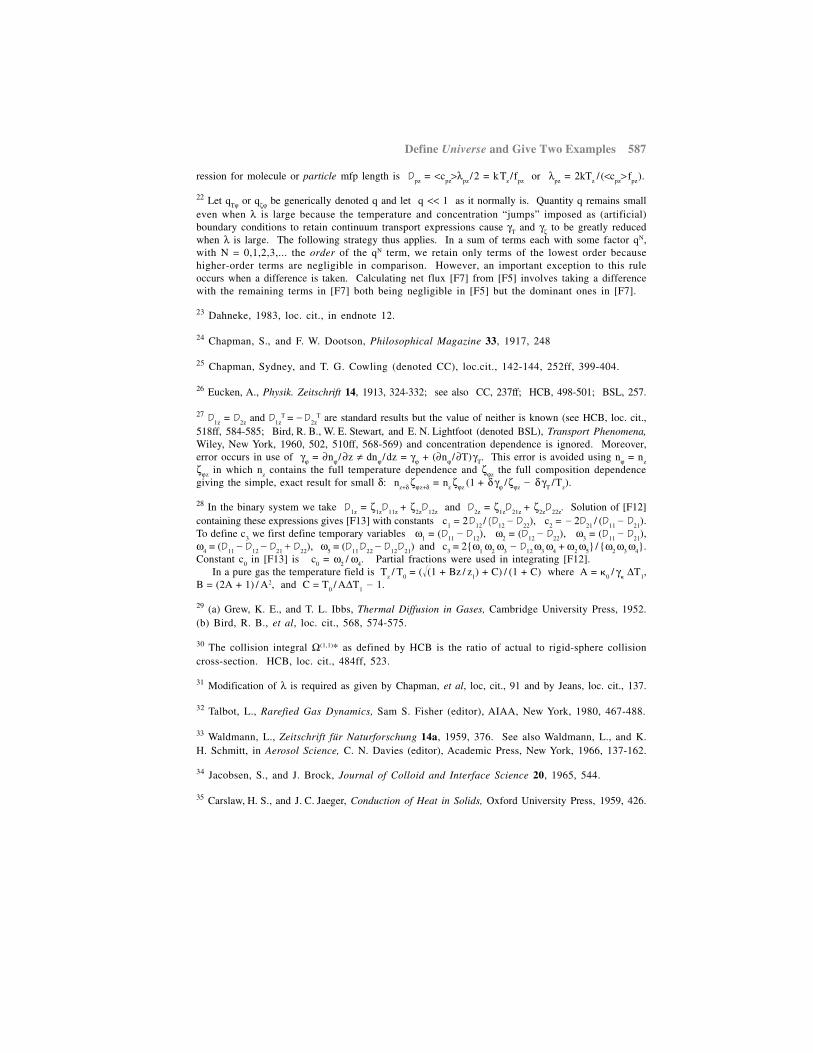
Define Universe and Give Two Examples 587
ression for molecule or particle mfp length is Dpz
= <cpz
>λpz
/ 2 = k Tz
/ fpz
or λpz
= 2kTz
/ (<cpz
> fpz
).
22 Let qTϕ or qζϕ be generically denoted q and let q << 1 as it normally is. Quantity q remains small
even when λ is large because the temperature and concentration “jumps” imposed as (artificial)boundary conditions to retain continuum transport expressions cause γ
T and γζ to be greatly reduced
when λ is large. The following strategy thus applies. In a sum of terms each with some factor qN,with N = 0,1,2,3,... the order of the qN term, we retain only terms of the lowest order becausehigher-order terms are negligible in comparison. However, an important exception to this ruleoccurs when a difference is taken. Calculating net flux [F7] from [F5] involves taking a differencewith the remaining terms in [F7] both being negligible in [F5] but the dominant ones in [F7].
23 Dahneke, 1983, loc. cit., in endnote 12.
24 Chapman, S., and F. W. Dootson, Philosophical Magazine 33, 1917, 248
25 Chapman, Sydney, and T. G. Cowling (denoted CC), loc.cit., 142-144, 252ff, 399-404.
26 Eucken, A., Physik. Zeitschrift 14, 1913, 324-332; see also CC, 237ff; HCB, 498-501; BSL, 257.
27 D1z
= D2z
and D1z
T = D2z
T are standard results but the value of neither is known (see HCB, loc. cit.,518ff, 584-585; Bird, R. B., W. E. Stewart, and E. N. Lightfoot (denoted BSL), Transport Phenomena,Wiley, New York, 1960, 502, 510ff, 568-569) and concentration dependence is ignored. Moreover,error occurs in use of γϕ = ∂ nϕ / ∂ z ≠ dnϕ / dz = γϕ + (∂ nϕ / ∂T) γ
T. This error is avoided using nϕ = n
z
ζϕz in which n
z contains the full temperature dependence and ζϕz
the full composition dependencegiving the simple, exact result for small δ: n
z+δ ζϕz+δ = nz
ζϕz (1 + δ γϕ / ζϕz
δ γT
/ Tz).
28 In the binary system we take D1z
= ζ1z
D11z
+ ζ2z
D12z
and D2z
= ζ1z
D21z
+ ζ2z
D22z
. Solution of [F12]containing these expressions gives [F13] with constants c
1 = 2 D
12 / (D
12 D
22), c
2 = 2D
21 / (D
11 D
21).
To define c3 we first define temporary variables ω
1 = (D
11 D
12), ω
2 = (D
12 D
22), ω
3 = (D
11 D
21),
ω4 = (D
11 D
12 D
21 D
22), ω
5 = (D
11 D
22 D
12 D
21) and c
3 = 2ω
1 ω
2 ω
3 D
12 ω
3 ω
4 + ω
2 ω
5 / ω
2 ω
3 ω
4.
Constant c0 in [F13] is c
0 = ω
2 / ω
4. Partial fractions were used in integrating [F12].
In a pure gas the temperature field is Tz
/ T0 = ((1 + Bz / z
1) + C) / (1 + C) where A =
0 / γ
∆T
1,
B = (2A + 1) / A2, and C = T0
/ A∆T1 1.
29 (a) Grew, K. E., and T. L. Ibbs, Thermal Diffusion in Gases, Cambridge University Press, 1952.(b) Bird, R. B., et al, loc. cit., 568, 574-575.
30 The collision integral Ω(1,1)* as defined by HCB is the ratio of actual to rigid-sphere collisioncross-section. HCB, loc. cit., 484ff, 523.
31 Modification of λ is required as given by Chapman, et al, loc, cit., 91 and by Jeans, loc. cit., 137.
32 Talbot, L., Rarefied Gas Dynamics, Sam S. Fisher (editor), AIAA, New York, 1980, 467-488.
33 Waldmann, L., Zeitschrift für Naturforschung 14a, 1959, 376. See also Waldmann, L., and K.H. Schmitt, in Aerosol Science, C. N. Davies (editor), Academic Press, New York, 1966, 137-162.
34 Jacobsen, S., and J. Brock, Journal of Colloid and Interface Science 20, 1965, 544.
35 Carslaw, H. S., and J. C. Jaeger, Conduction of Heat in Solids, Oxford University Press, 1959, 426.