1

NASA Contract Report NAS1-00086-A003

Computation of Sound Propagation by Boundary Element Method Yueping Guo The Boeing Company Mail Code H013-B308 5301 Bolsa Avenue Huntington Beach, CA 92647 yueping.guo@boeing.com

September 2005 National Aeronautics and Space Administration Langley Research Center Hampton, VA 23681

https://ntrs.nasa.gov/search.jsp?R=20080030156 2018-06-25T04:59:58+00:00Z

2

Table of Contents

1. Introduction................................................................................................................. 5

2. Governing Equations .................................................................................................. 7

3. Numerical Scheme.................................................................................................... 11

4. Sound Scattering by a Sphere................................................................................... 14

5. Sound Reflection by a Plate with Uniform Flow...................................................... 17

6. Sound Propagation over a Hump.............................................................................. 20

7. Far Field Formulation............................................................................................... 22

8. Calculation of Derivatives........................................................................................ 23

9. Conclusions............................................................................................................... 25

Nomenclature.................................................................................................................... 26

List of Figures................................................................................................................... 27

References......................................................................................................................... 28

3

Acknowledgments

The work reported here was conducted under NASA Contract NAS1-00086, under the Quiet Aircraft Technology (QAT) program. The author would like to thank the task monitor, Dr. Mehdi Khorrami of NASA LaRC, for his support and encouragement.

4

Abstract

This report documents the development of a Boundary Element Method (BEM) code for the computation of sound propagation in uniform mean flows. The basic formulation and implementation follow the standard BEM methodology; the convective wave equation and the boundary conditions on the surfaces of the bodies in the flow are formulated into an integral equation and the method of collocation is used to discretize this equation into a matrix equation to be solved numerically. New features discussed here include the formulation of the additional terms due to the effects of the mean flow and the treatment of the numerical singularities in the implementation by the method of collocation. The effects of mean flows introduce terms in the integral equation that contain the gradients of the unknown, which is undesirable if the gradients are treated as additional unknowns, greatly increasing the sizes of the matrix equation, or if numerical differentiation is used to approximate the gradients, introducing numerical error in the computation. It is shown that these terms can be reformulated in terms of the unknown itself, making the integral equation very similar to the case without mean flows and simple for numerical implementation. To avoid asymptotic analysis in the treatment of numerical singularities in the method of collocation, as is conventionally done, we perform the surface integrations in the integral equation by using sub-triangles so that the field point never coincide with the evaluation points on the surfaces. This simplifies the formulation and greatly facilitates the implementation. To validate the method and the code, three canonic problems are studied. They are respectively the sound scattering by a sphere, the sound reflection by a plate in uniform mean flows and the sound propagation over a hump of irregular shape in uniform flows. The first two have analytical solutions and the third is solved by the method of Computational Aeroacoustics (CAA), all of which are used to compare the BEM solutions. The comparisons show very good agreements and validate the accuracy of the BEM approach implemented here.

5

1. Introduction

In practical applications such as airframe noise prediction, noise propagation very often involves complex geometry, the effects of which can only be dealt with by numerical methods. There are various numerical methods studied in the past, including the Boundary Element Method (BEM). Though the basic theories of these methods are well established, their applications to practical problems are limited by their heavy requirements on computation resources. Compared with other numerical methods, BEM has the advantageous feature of only involving surface discretization, making the numerical computation less demanding, both in computation time and in data storage. Because of this, BEM plays an important and useful role in practical applications of noise prediction. In this report, we document the formulation, implementation and validation of a BEM code.

The Boundary Element Method has been an active research topic for many years and the fundamental theory and formulation have been well established and documented in the open literature (e.g. Ref 1 to Ref 7). Thus, it is appropriate to point out that the work reported here is not intended to provide any new break through in this topic. The objective of this report is twofold. The first is to provide a document for the implementation and validation of this method with all the relevant technical details so that it serves as a user manual. Our second objective is to discuss a few features related to the implementation of BEM that do not seem to have reported in the open literature. These include a treatment of the mean flow effects to eliminate the gradients of the unknown in the integral equation, a discretization scheme that is free of numerical singularity and a formulation that computes the high order spatial derivatives of the solution. Again, these features are not fundamental break through of BEM, but they facilitate its implementation and provide incremental improvement to the method.

The formulation of BEM is well established. It involves converting the governing equation, the convective wave equation for applications with uniform mean flow, and the boundary condition, the vanishing of the normal derivative of the unknown on the surfaces of bodies embedded in the flow, into an integral equation on the body surfaces through the application of the Greens theorem. The integral equation is solved numerically by discretizing it into a matrix equation, which leads to solutions of the unknown on the surfaces. Solutions in the field can then be found from these surface solutions by integration. In the integral equation formulation, both the unknown and its gradients appear in the integrand in cases of non-zero uniform mean flow. Traditionally, this is dealt with by one of the two approaches. One is to differentiate the integral equation to derive an additional set of equations so that both the unknown and its gradients are solved simultaneously by two sets of coupled matrix equations. Clearly, compared with the cases without mean flow where only the unknown itself is solved, this approach significantly increases the computation time and storage requirement, by doubling the dimension, and hence quadrupling the size, of the matrix equation to be solved. The second approach to deal with the gradients of the unknown in the integral equation is to approximate the

6

gradients numerically, by finite differencing, for example, so that the integral equation reduces to one that only contains the unknown itself. While this approach does not increase the dimensions of the matrix equation to be solved, it relates the unknown at a surface point to those at its neighboring points in the integral equation, making the discretization scheme and coding more complex. It also introduces additional numerical error in approximating the derivatives by numerical differencing.

In this report, we will present a different approach that avoids the disadvantages of the two previous approaches. We will show that the terms involving the gradients of the unknown in the integral equation can be reformulated in terms of the unknown itself. By this reformulation, the integral equation to be solved only involves the unknown itself and the structure of the integral equation is very similar to that for cases without mean flow. The reformulation is exact and does not involve any numerical differentiation. This is clearly advantageous and desirable, both ensuring the accuracy of the approach and minimizing the requirement of computation resources.

There are many ways to discretize the integral equation in BEM for numerical solution, as extensively discussed and review in the literature. The methods range from the collocation method to the spectral method, the former corresponding mathematically to the use of a local weight in the kernel of the integral equation and the latter to the use of a global weight. Each of these methods has its advantages and disadvantages. We choose to work with the collocation method because of its ease of implementation. To avoid its disadvantage of having to deal with numerical singularities when the solution point coincides with one of the surface integration points, we carry out the surface integration by further dividing each of the discretized individual surface elements into sub-triangles. When numerically calculating the surface integration on an element, by summing the products of the integrand values and the sub-triangle surface areas, the solution point and the surface integration points never coincide because the former is one of the vertexes of the triangles and the latter is their geometric centers. This eliminates the need for asymptotic analysis of the integral equation, as necessary in typical implementation of BEM by collocation method.

One application of BEM is as a Greens function solver to compute the propagation effects of sound waves in the prediction of noise from unsteady flows. In such applications, it is often required to compute the derivatives of the Greens function (Ref 8 to Ref 10). It can in theory be done by numerical differentiation once the Greens function itself is found in all spatial domains. This, however, is not the preferred approach, both because of the extra computation time required to carry out the numerical differentiation and because of the accumulated numerical errors in the final results. The latter is probably the more serve limitation of the two, especially with non-uniform spatial grid and low order schemes of numerical differentiation. These limitations can be overcome by computing the high order derivatives of the Greens function directly from the solutions of the Greens function on the body surfaces, namely, the

7

solutions of the BEM matrix equation. In this report, we derive the formulas for computing the high order derivatives, which, though not difficult, is quite involved and tedious.

To validate the BEM approach and the implemented code, we choose to study three canonical problems. The first is the sound scattering from a rigid sphere in a static medium. Clearly, this problem is considered here because of the availability of analytical solutions, as studied and documented extensively in the literature. The analytical solutions provide a good validation with minimum uncertainty. The problem, however, is only for static medium without mean flows. For problems with both mean flows and boundary surfaces present, exact analytical solutions basically do not exist. Our validation will then rely on approximate solutions and on comparisons with other numerical methods. For this purpose, we also use a numerical code, based on the methods of Computational Aeroacoustics (CAA), to study the second and third canonic problem, which are respectively the sound reflection from a large flat plate, placed in parallel with the direction of a uniform mean flow, and the sound propagation over a hump in a uniform mean flow. For a plate whose dimensions are large compared with the sound wavelength, the solutions away from the plate edges are not significantly affected by the edges so that the analytical solution for an infinity plate serves as a good approximation to the finite plate solution. By studying this problem by both CAA and BEM, and comparing the results with the approximate analytical solutions, not only the BEM code gets validated for a case with mean flow, but also the relevance of the CAA code is established so that it can provide comparisons in cases where even approximate solutions are not available. Our third validation is such a case, where sound waves propagate over an irregularly shaped hump in a mean flow. In this case, the validation of BEM solutions entirely replies on the comparisons between BEM and CAA. As will be seen in subsequent sections, all three validation cases show good accuracy of the BEM solutions.

2. Governing Equations

When applying BEM to acoustic problems, we seek to solve the convective wave equation in frequency domain in the form of,

( ) ),(i 220 xM qggk =∇−∇⋅+− (2.1)

where g is the unknown to be solved, which can be regarded as the velocity potential, and q can be any source distribution. We have introduced k0 and M to respectively denote the acoustic wavenumber and the vector mean flow Mach number. The acoustic wavenumber k0 is related to the angular frequency � and sound speed c0 by

,/ 00 ck ω= (2.2)

and the vector Mach number M is defined by the flow velocity U by

8

./ 0cUM = (2.3)

The governing equation (2.1) is defined by the Cartesian coordinate system

{ },,, 321 xxx=x (2.4)

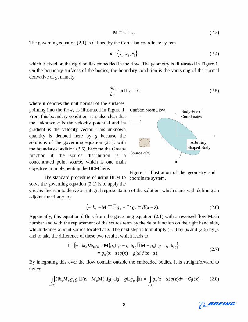
which is fixed on the rigid bodies embedded in the flow. The geometry is illustrated in Figure 1. On the boundary surfaces of the bodies, the boundary condition is the vanishing of the normal derivative of g, namely,

,0=∇⋅=∂∂

gn

gn (2.5)

where n denotes the unit normal of the surfaces, pointing into the flow, as illustrated in Figure 1. From this boundary condition, it is also clear that the unknown g is the velocity potential and its gradient is the velocity vector. This unknown quantity is denoted here by g because the solutions of the governing equation (2.1), with the boundary condition (2.5), become the Greens function if the source distribution is a concentrated point source, which is one main objective in implementing the BEM here.

The standard procedure of using BEM to solve the governing equation (2.1) is to apply the Greens theorem to derive an integral representation of the solution, which starts with defining an adjoint function g0 by

( ) ).(i 02

02

0 zxM −=∇−∇⋅−− δggk (2.6)

Apparently, this equation differs from the governing equation (2.1) with a reversed flow Mach number and with the replacement of the source term by the delta function on the right hand side, which defines a point source located at z. The next step is to multiply (2.1) by g0 and (2.6) by g, and to take the difference of these two results, which leads to

( ){ }).()()()(

i2

0

000000

zxxxzx

MMM

−−−=∇+∇−⋅∇−∇+−⋅∇

δgqg

ggggggggggk (2.7)

By integrating this over the flow domain outside the embedded bodies, it is straightforward to derive

( )[ ] ).()()()(i2)(

0

)(

0000 xzxzMnzz

CgdvqgdsggggMggMkVS

nn −−=∇−∇⋅−+ (2.8)

n

Uniform Mean Flow Body-FixedCoordinates

Arbitrary Shaped Body

Source q(x)

Figure 1 Illustration of the geometry and coordinate system.

9

Here the left hand side follows from the use of the divergence theorem, which reduces the volume integration over the left hand side of (2.7) to a surface integration. The surfaces of the all the rigid bodies in the flow are collectively denoted by S(z), with differential surface element ds, and the component of the mean flow Mach number in the surface normal direction is denoted by Mn, namely,

.Mn ⋅=nM (2.9)

The right hand side of the result (2.8) contains a volume-integration over the source distribution q, with the differential volume element denoted by dv. The last term in the right hand side results from the trivial application of the delta functions to carry out the volume-integration. In carrying out this integration, the coefficient C is introduced to account for the three cases where the field point x is respectively inside, on the boundary surface and outside the flow. Its values are given by

�����

=flow outside for 0

surfaceboundary on for 5.0

flowin for 1

x

x

x

C (2.10)

which is well-known in BEM formulations and accounts for the singular nature of the surface integral when the field points are on the surface.

Now the boundary condition (2.5) can be applied to simplify the result (2.8) by eliminating terms involving the normal derivatives of g, which leads to

( )[ ] .i2

)()()(

)(

00000

)(

0

∇⋅−∇⋅−∇⋅+−

−=

z

z

MnM

zxzx

S

nnn

V

dsgMgggMgMkg

dvqgCg

(2.11)

It should be noted that the gradients inside the surface integration are with respect to the coordinate z. This is the integral equation to be solved for the function g. It can be seen that the integral on the right hand side not only contains the unknown function g, but also its gradients, respectively in the two terms in the integrand. Apparently, the gradient term is due to the presence of the uniform mean flow since the term involving the gradient of the unknown is proportional to the mean flow Mach number. In a static acoustic medium, this term vanishes and the integral is entirely given by the function g itself.

To solve the equation (2.11) numerically, it is desirable to have only g as the unknown without the term involving its derivatives. This term can be further manipulated by writing the vector Mach number M and the gradient of g in a body-fitted coordinate system that has two components on the body surface and the surface normal as its third component. In this coordinate system, we have

10

,ggn

gMg ssssn ∇⋅=∇⋅+

∂∂=∇⋅ MMM (2.12)

where the last step follows from the use of the boundary condition (2.5) and the subscript s denotes the two coordinates in the two tangential directions on the surface (s = 1, 2). These surface coordinates can be defined as the arc lengths on the surface, but in vector form, a surface quantity can be simply written as the difference between the full vector and its normal component. Thus, we have the definitions

.andn

M sns ∂∂−∇=∇−= nMM (2.13)

From (2.12), the last term in (2.11) becomes

( ) ( )[ ] .)(

00

)(

0

)(

0

⋅∇−⋅∇=

∇⋅=∇⋅

z

zz

MM

MM

S

snssns

S

ssn

S

n

dsMgggMg

gdsMggdsMg

(2.14)

The first term in the above result is in a divergence form, in terms of the surface coordinates, which integrates to zero for finite bodies with closed surfaces. The last term only involves g as the unknown. Thus, the integral equation (2.11) reduces to the compact form

),()(),()()(

xzxzxz

QdsgACgS

=+ (2.15)

where Q is written for

,)()()(

0 dvqgQV

−=z

zxz (2.16)

and the quantity A denotes

( ).)(i2 0000 snsnn MggMgMkA MnM ⋅∇+∇⋅−+= (2.17)

Apparently, the result (2.15) is an integral equation with g as the only unknown.

To proceed from here, the adjoint function g0 must be found, as the solution to (2.6) in an infinity space. The solution to this equation can be found easily by standard procedures (e.g. Ref 11 and 12) in the form of

( ) ,4

1)(

20 /)(i

0β

πxzMxz −⋅+

∗

∗

=− RkeR

g (2.18)

where R∗ denotes

( ) ,)( 222 Mxzxz ⋅−+−=∗ βR (2.19)

11

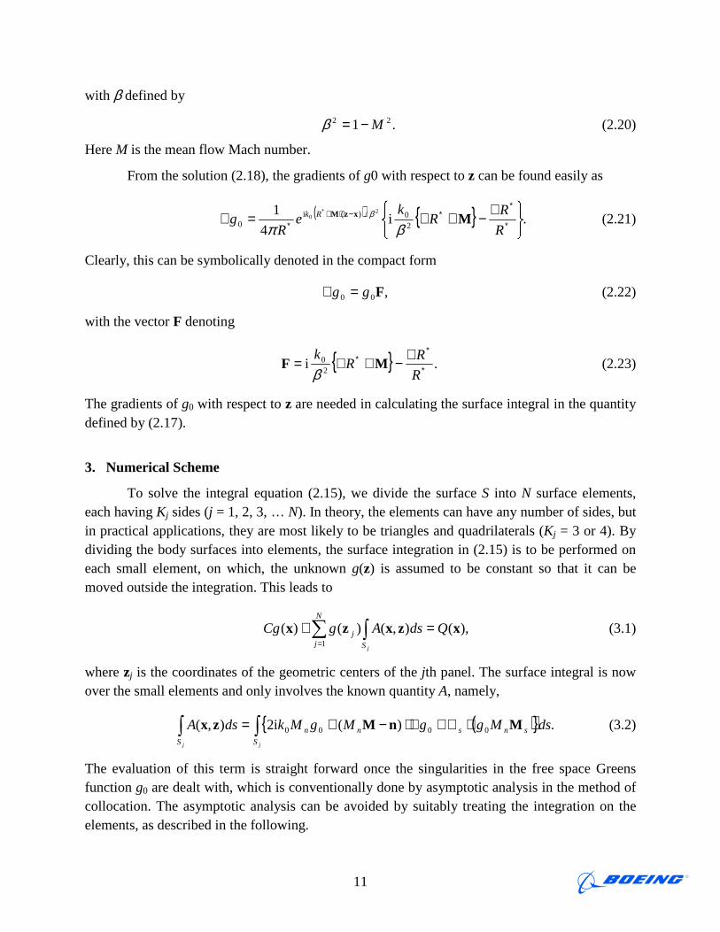
with β defined by

.1 22 M−=β (2.20)

Here M is the mean flow Mach number.

From the solution (2.18), the gradients of g0 with respect to z can be found easily as

( ) { } .i4

120/)(i

0

20 ���

����� ∇−+∇=∇ ∗

∗∗−⋅+

∗

∗

R

RR

ke

Rg Rk MxzM

βπβ (2.21)

Clearly, this can be symbolically denoted in the compact form

,00 Fgg =∇ (2.22)

with the vector F denoting

{ } .i20

∗

∗∗ ∇−+∇=

R

RR

kMF

β (2.23)

The gradients of g0 with respect to z are needed in calculating the surface integral in the quantity defined by (2.17).

3. Numerical Scheme

To solve the integral equation (2.15), we divide the surface S into N surface elements, each having Kj sides (j = 1, 2, 3, … N). In theory, the elements can have any number of sides, but in practical applications, they are most likely to be triangles and quadrilaterals (Kj = 3 or 4). By dividing the body surfaces into elements, the surface integration in (2.15) is to be performed on each small element, on which, the unknown g(z) is assumed to be constant so that it can be moved outside the integration. This leads to

),(),()()(1

xzxzx QdsAgCgjS

N

jj =+

=

(3.1)

where zj is the coordinates of the geometric centers of the jth panel. The surface integral is now over the small elements and only involves the known quantity A, namely,

( ){ } .)(i2),( 0000 ⋅∇+∇⋅−+=jj S

snsnn

S

dsMggMgMkdsA MnMzx (3.2)

The evaluation of this term is straight forward once the singularities in the free space Greens function g0 are dealt with, which is conventionally done by asymptotic analysis in the method of collocation. The asymptotic analysis can be avoided by suitably treating the integration on the elements, as described in the following.

12

To this end, we start with the first two terms in the integrand of (3.2) and divide the element Sj into Kj sub-triangles by connecting each vertex of the element with its geometric center zj, as illustrated in Figure 2. The integration over an individual sub-triangle can then be done by evaluating the integrand function at the geometric center of the triangle and multiplying the result by its area. The total integration over the jth element, namely, over Sj, is of course the summation over all the sub-triangles. For the first two terms in the integrand of (3.2), this leads to the result

{ } ,)~()()~(i21

000=

−∇⋅−+−jK

kkknkn sgMgMk zxnMzx (3.3)

where the summation is over the number of sub-triangles in the element, which equals to the number of sides. For the kth sub-triangle (k = 1…Kj), its geometric center and surface area are respectively denoted by kz~ and sk. Both are

illustrated in Figure 2.

For the last term in the integrand of (3.2), the divergence can be used to reduce the surface integration to line integration, along the sides of the element. Each line integral can then be evaluated by the value of the integrand function at the center of the line segment multiplied by the length of the segment. This leads to

,)(1

0=

⋅−jK

kkksnk aMg nMzx (3.4)

where kz is the center of the kth side of the element, kn is its normal, in the same plane as the

sub-triangle and pointing outward away from the element, and ak is its length. Again, these definitions are illustrated in Figure 2.

By collecting (3.3) and (3.4), the surface integration in (3.1) becomes a summation over the number of sides of the jth panel in the form of

{ }[ ].)()~()()~(i21

0000=

⋅−+−∇⋅−+−=j

j

K

kkksnkkknkn

S

aMgsgMgMkAds nMzxzxnMzx (3.5)

In this result, the quantities that depend on the individual sub-triangles are explicitly indicated by the subscript k. The quantity Mn, defined by (2.9), is also evaluated for each sub-triangle because the surface normal can vary within each element. Thus, the surface normal n should be evaluated for each sub-triangle in the surface integration.

jth Surface Element kth Sub-Triangle

kz~kz

knjz

normal sideth center sideth

center eth triangl~centerelement th

kkkj

k

k

k

j

====

nzzz

Figure 2 Geometry and definitions of a surface element and its sub-triangles

13

The result (3.5) gives the surface integration on the jth surface element, whose surface is denoted by Sj and on which the solution of g is assumed to be constant and represented by its value at the geometric center of the surface element zj. The result is valid for any point x so that, when substituted into (3.1), it can be used to compute field solutions as well as solutions on the surfaces. The matrix equation to solve for g can be constructed by setting (3.1) to the geometric centers of the surface elements. This leads to a matrix equation in the form of

,2

1

1i

N

jjiji Qgg =+

=

α (3.6)

which unknowns of the equation are gi, defined by

),( ii gg x= (3.7)

with xi being the coordinates of the geometric centers of the ith surface element. The source terms of (3.6) are similarly defined by

),( ii QQ x= (3.8)

and the coefficients of the matrix equation is given by

,),(=jS

iij dsA zxα (3.9)

namely, given by (3.5) with x replaced by xi. It can be noted that when using (3.5) to calculate the coefficients of the matrix equation (3.6), the adjoint the free space Greens function has to be computed in the forms

).(and)~( 00 kiki gg zxzx −− (3.10)

Since the three position vectors in these respectively denote the geometric center of the ith panel, the geometric center of the kth sub-triangle of the jth panel and the center of the kth side of the jth panel, the three points never coincide, even in the case of i = j, which is very desirable in numerical implementation because the computation of the matrix coefficients is always free of singularity.

In comparison with various BEM formulations and implementations, the formulations given in this section and the previous section have two main attractive features. One is that the integral equation does not involve the gradients of the unknown, which limits the requirement on computation resources to the same as that for the cases without mean flow, both when solving the matrix equation for the solutions on the surfaces and when performing the surface integration to find solution in the field. The second attractive feature is that the coefficients of the matrix equation is always free of numerical singularities, even though the discretization of the integral

14

equation follows the approach of co-location, which usually requires asymptotic analysis to avoid singularities. These two features make the implementation very straightforward.

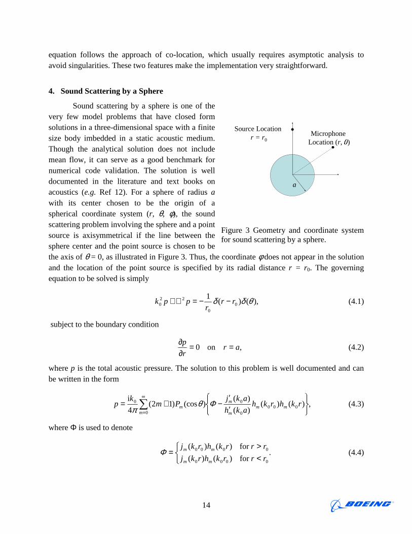
4. Sound Scattering by a Sphere

Sound scattering by a sphere is one of the very few model problems that have closed form solutions in a three-dimensional space with a finite size body imbedded in a static acoustic medium. Though the analytical solution does not include mean flow, it can serve as a good benchmark for numerical code validation. The solution is well documented in the literature and text books on acoustics (e.g. Ref 12). For a sphere of radius a with its center chosen to be the origin of a spherical coordinate system (r, θ, φ), the sound scattering problem involving the sphere and a point source is axisymmetrical if the line between the sphere center and the point source is chosen to be the axis of θ = 0, as illustrated in Figure 3. Thus, the coordinate φ does not appear in the solution and the location of the point source is specified by its radial distance r = r0. The governing equation to be solved is simply

),()(1

00

220 θδδ rr

rppk −−=∇+ (4.1)

subject to the boundary condition

,on0 arr

p ==∂∂

(4.2)

where p is the total acoustic pressure. The solution to this problem is well documented and can be written in the form

,)()()(

)()(cos)12(

4

i000

0

0

0

0 � ��

�� � ′′

−+=∞

=rkhrkh

akh

akjPm

kp mm

m

m

mm Φθ

π (4.3)

where Φ is used to denote

.for )()(

for )()(

0000

0000�� �<>

=rrrkhrkj

rrrkhrkj

mm

mmΦ (4.4)

Source Location r = r0

Microphone Location (r, � )

a

Figure 3 Geometry and coordinate system for sound scattering by a sphere.

15

This term corresponds to the standard solution for a point source of angular frequency � , which determines the acoustic wavenumber by k0. The solution is in terms of the spherical coordinate system (r, θ, φ). The expanded solution is expressed by the Lagrange polynomial Pm of order m and the spherical Bessel and Hankel function of order m, respectively denoted by jm and hm. The prime over the spherical Bessel and Hankel functions indicates differentiation with respect to their argument. This solution can be easily computed with the summation truncated at some large number. The terms in the summation become progressively smaller so that the truncation only leads to a small error in the final results.

The problem defined by (4.1) and (4.2) is solved by BEM to validate the BEM code (setting the mean flow to zero). Some comparisons are given in Figure 4 to Figure 7. In all the comparisons, the source location is set at r0 = 4a and the analytical solutions are computed from (4.3) and (4.4). Figure 4 shows comparisons at two field locations; the upper diagram is for a location in the insonified region on the same side of the sphere as the source at r = 5a and � = 0, and the lower diagram for a location in the shadow region at r = 5a and � = � . Both diagrams plot the real part of p (in red color), the imaginary part of p (in green) and its amplitude (in blue), as a function of the non-dimensional frequency k0a. The symbols are the results of the BEM computations and the curves are the analytical solutions. Apparently, the agreement between the two is very good, not only in the insonified region where the direct radiation from the source dominates, but also in the shadow region where the dominant noise is from the scattering of the sphere. This illustrates the accuracy of the BEM method implemented here.

k0a0 2 4 6 8 10

-0.1

-0.05

0

0.05

0.1

Re(p) Im(p)

k0a0 2 4 6 8 10

-0.02

-0.01

0

0.01

0.02Re(p) Im(p)

Figure 4 Comparisons between BEM (symbols) and analytical solutions (curves), with the upper and lower plot respectively for � = 0 and � = � , both for r = 5a.

0

30

6090

120

150

180

210

240270

300

330

AnalyticalBEM

Figure 5 Directivity comparisons for scattering by a sphere on the circle r = 1.5a for k0a = 9.24.

16

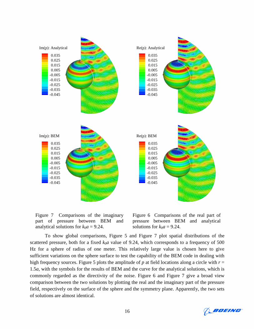
To show global comparisons, Figure 5 and Figure 7 plot spatial distributions of the scattered pressure, both for a fixed k0a value of 9.24, which corresponds to a frequency of 500 Hz for a sphere of radius of one meter. This relatively large value is chosen here to give sufficient variations on the sphere surface to test the capability of the BEM code in dealing with high frequency sources. Figure 5 plots the amplitude of p at field locations along a circle with r = 1.5a, with the symbols for the results of BEM and the curve for the analytical solutions, which is commonly regarded as the directivity of the noise. Figure 6 and Figure 7 give a broad view comparison between the two solutions by plotting the real and the imaginary part of the pressure field, respectively on the surface of the sphere and the symmetry plane. Apparently, the two sets of solutions are almost identical.

0.0350.0250.0150.005

-0.005-0.015-0.025-0.035-0.045

Im(p): Analytical

0.0350.0250.0150.005

-0.005-0.015-0.025-0.035-0.045

Im(p): BEM

Figure 7 Comparisons of the imaginary part of pressure between BEM and analytical solutions for k0a = 9.24.

0.0350.0250.0150.005

-0.005-0.015-0.025-0.035-0.045

Re(p): Analytical

0.0350.0250.0150.005

-0.005-0.015-0.025-0.035-0.045

Re(p): BEM

Figure 6 Comparisons of the real part of pressure between BEM and analytical solutions for k0a = 9.24.

17

5. Sound Reflection by a Plate with Uniform Flow

When mean flows are present, closed form analytical solutions usually do not exist. Approximate analytical solutions may be found for simply geometries, one example being sound reflection by a large plate in a uniform flow. The solution is exact for an infinite plate, but for comparisons with numerical methods such as BEM and CAA which can only treat finite plates, the solution can be used in the region away from the edges of the plate. The sound field in this region is almost the same as that from an infinity plate and the analytical solution for an infinite plate provides a good approximation to the finite plate problem.

The governing equation for the sound reflection problem is

( ) ),(~)(i 022

0 ωδ qppk xxM −=∇−∇⋅+− (5.1)

where M is the mean flow Mach number and x0 is the source location. Without loss of generality, we can choose the Cartesian coordinate system x such that two of the three axes are on the plate and the point source is on the axis perpendicular to the plate. The source location is then specified by the distance between the plate and the source, denoted by h, and the location vector becomes

} .,0,0{0 h=x (5.2)

Accordingly, the mean flow is in the positive x1 direction and the mean flow Mach number is given by

} .0,0,{ M=M (5.3)

In this coordinate system, the boundary condition is simply the vanishing of the normal derivative of p on the plate, expressed by,

.0on0 33

==∂∂

xx

p (5.4)

The geometry and the coordinate system are illustrated in Figure 8.

In the governing equation (5.1), we have defined the source amplitude by a frequency dependent quantity, given by

Uniform Mean FlowSource Location

(0, 0, h)

Flat Plate

Figure 8 Illustration of the geometry and coordinate system for the problem of sound reflection by a plate in a uniform flow.

18

�������

≥

≤<−

≤

=

2||0

2||12

)1|(|cos

1||1

)(~

0

00

0

ak

akak

ak

qπω (5.5)

where k0 is the acoustic wavenumber as defined before and a is a length scale. This particular source definition is used here, instead of the unity constant amplitude, because it corresponds to a regular function in time domain. For unity constant amplitude, the time domain source would be a singular delta function. Since we also use a code based on CAA methods to solve this problem and the CAA code is in time domain, the regular source function is used to facilitate the CAA computation. This actually has no impact on the BEM calculations which are in frequency domain; the amplitude can be multiplied to the BEM solutions of unity amplitude, as a trivial step in the post processing of the BEM solutions. To illustrate the properties of the source definition (5.5), the source function is plotted in Figure 9, as a function of the non-dimensional frequency k0a.

The analytical solution can be found very easily for an infinite plate. In this case, the reflection of the point source is simply its mirror image, which ensures the vanishing of the total normal velocity on the plate. Thus, the solution to the governing equation (5.1) and (5.4) can be written as

( ) ( ) ,~4

)(~

4

)(~2

002

00 /)~(~

i/)(i ββ

πω

πω xxMxxM −⋅−

∗−⋅−

∗

∗∗

+= RkRk eR

qe

R

qp (5.6)

where R∗ is given by (2.19) and the tilde over it indicates that it is calculated with x0 replaced by its image point

} .,0,0{~0 h−=x (5.7)

It can be seen that the solution is basically in terms of the function g0 defined in previous sections, but with the flow direction reversed.

k0a

q(ω

)

0 0.5 1 1.5 2 2.5 30

0.2

0.4

0.6

0.8

1

Figure 9 Illustration of the source function used in the CAA computation

k0a0 0.5 1 1.5 2

-0.04

-0.02

0

0.02

0.04

Re Im

Figure 10 Comparisons between analytical (curves), BEM (closed symbols) and CAA (open symbols) solutions for M = 0.2 at the surface location (-2, 0, 0) for a source located at h = 5.

19

The validation for the problem of sound reflection is done with comparisons between three methods, namely, the analytical solution (5.6), the BEM results and the CAA computations. In all the comparisons, the source is located above the plate at h = 5 and the mean flow Mach number is M = 0.2. To illustrate the comparisons, Figure 10 plots the convective derivative of the pressure, namely, the quantity,

.i 0 ppkDt

Dp ∇⋅+−= M (5.8)

This quantity is plotted here because it is the direct output of the CAA code. The results in Figure 10 are from the three methods at the surface location (-2, 0, 0) as a function of the non-dimensional frequency k0a, with the analytical solution plotted by the curves, the BEM results by the closed symbols and the CAA results by the open symbols. Both the real and the imaginary part, respectively denoted by the squares and the diamonds, are plotted in this figure and both show very good agreement between the three methods.

Analytical

M = 0.2

BEM

M = 0.2

M = 0.2

CAA

-0.015 -0.005 0.005 0.015 0.025

Re(p)

Figure 11 Comparisons between analytical, BEM and CAA solutions for M = 0.2 on a vertical plane through the source location for the real part of the acoustic pressure.

Analytical

M = 0.2

BEM

M = 0.2

M = 0.2

CAA

-0.015 -0.005 0.005 0.015 0.025

Re(p)

Figure 12 Comparisons between analytical, BEM and CAA solutions for M = 0.2 on the plate for a source located at h = 5 for the real part of the acoustic pressure.

20

More comparisons are given in Figure 11 and Figure 11 for the real part of the acoustic pressure at the non-dimensional frequency k0a = 0.93 with the mean flow Mach number of 0.2 and the source location h = 5. Similarly to the comparisons in Figure 10, the agreement between the three methods is very good, except for the regions near the edges of the plate where the CAA solutions show discrepancies with the other two methods. This is actually expected because the CAA method uses absorptive boundary conditions at the computational boundaries to prevent the wave being reflected back to the computational domain. Thus, the waves are heavily dissipated in the regions near the edges, as is clearly from the lower diagrams of both Figure 11 and Figure 11. Comparisons for the imaginary part of the acoustic pressure have equally good agreement, though not plotted here.

6. Sound Propagation over a Hump

This section describes the validation of the BEM approach through a problem with irregular geometry, which is a hump on a plate. Without loss of generality, the hump is specified by a Gaussian curve of the form

,2 )(05.03

22

21 xxex +−= (6.1)

which assumes its maximum at the origin of the coordinate system with a values of 2 and decays away from this maximum with a rate of 0.05. The geometry is shown in Figure 13. The governing equation for this problem is also given by (5.1), as in the sound reflection problem discussed in the previous section, and the boundary condition of zero normal velocity on the curved surface is now specified by

,0=∂∂=∇⋅n

ppn (6.2)

on the surface defined by (6.1).

Apparently, there is no analytical solution for such a problem so that the validation in this section will depend on comparisons with results from numerical solutions by CAA, which is also used in the previous section for the flat plate problem. The flap plate problem serves as an intermediate step to establish the relevance of the CAA code, which itself needs validation since it is also a numerical solution code. By first studying the flat plate problem that has analytical solution, both the CAA code and the BEM code are validated. A general curved surface problem is also

M

Source (-5, 0, 5)

Figure 13 Geometry and coordinate system for the problem of sound propagation over a hump in a uniform flow.

21

needed to validate the BEM approach, as in this section, because the flat plate problem, as well as the scattering by a sphere without mean flow, does not validate all terms in the BEM formulation. It is clear that the case without mean flow cannot validate any terms involving mean flows in the BEM formulation (2.17). It can also be seen that this same group of terms are also all identically zero in the flat plate case, because the mean flow is in parallel to the plate so that the component of the flow velocity in the direction of the plate normal, defined by Mn, is identically zero. Thus, even though the flat plate problem has mean flow included, the terms in the BEM formulation are not fully validated by this canonic problem, which is why a more general curved surface problem is chosen to be studied in this section.

Similarly to the other two validation cases in the two previous sections, the comparisons between BEM and CAA for the irregular hump problem show good agreement. To illustrate this, some examples are plotted in Figure 14 and Figure 15 for the real part of the acoustic pressure with the mean flow Mach number M = 0.2, the source location h = 5 and the non-dimensional frequency k0a = 0.98. The two figures are respectively for the curved surface and a vertical plane cutting through the source location. The good agreement is evident and again discrepancies are seen in the regions close to the edges of the plate, due to the use of absorptive numerical boundary condition for the computational domain in the CAA computations, as discussed in the previous section.

BEM

M = 0.2

M = 0.2

CAA

-0.015 -0.005 0.005 0.015 0.025

Re(p)

Figure 15 Comparisons between BEM and CAA solutions on a vertical plane for the real part of the acoustic pressure.

BEM

M = 0.2

M = 0.2

CAA

-0.015 -0.005 0.005 0.015 0.025

Re(p)

Figure 14 Comparisons between BEM and CAA solutions on the surface of a Guassian hump for the real part of acoustic pressure.

22

7. Far Field Formulation

In many practical applications, the sources of the noise and the microphone locations are usually far apart from each other, separated by many wavelengths. In this case, the far field approximation can be used to simplify the computations. Thus, a form of the BEM formulation with far field applications is given in this section. In the notation used in previous sections, the far field condition means that the field point x is far away from the source point z, namely,

.zx >> (7.1)

Thus, the usual far field limit can be applied to g0(z-x) that is used in the BEM formulation and defined by (2.18). The far field approximation essentially neglects the variations due to z in the amplitude and expends the phase function in a power series. The amplitude of (2.18) is then approximated as

,4

1

)(||4

1

4

1222 ∗

∞∗ =

⋅+≈

RR πβππ xMx (7.2)

where the subscript ∞ on the quantity R∗ denotes its value in the far field,

,||)(|| 22222rMR +=⋅+=∗

∞ ββ xxMx (7.3)

where we have used Mr to denote the component of the mean flow Mach number in the direction of the far field point x. It is defined by

,x̂M ⋅=rM (7.4)

with the far field the directivity vectors defined by

.||/ˆ xxx = (7.5)

The phase function (2.18) can be correspondingly expanded as

( ) ,2

0 /i β�zxM ⋅−⋅−∗

∞Rke (7.6)

where the dependence of the phase function on the source coordinate z is explicitly factored out and the vector quantity ΦΦΦΦ is defined by

.)(ˆ

22

222

r

rr

M

MM

+

+−+=

β

ββ Mx (7.7)

Apparently, this is a function of the far field coordinate x only.

With all these, the free space Greens function g0(z-x) defined by (2.18) can now be written as

,)()(2

0 /i00

β�zxxz ⋅−=− keAg (7.8)

23

where A0 is an amplitude that only depends on the far field coordinate x, given by

( ) .4

1)(

20 /i

0β

πxMx ⋅−

∗∞

∗∞= Rke

RA (7.9)

The far field form of the free space Greens function allows us to factor out the large distance in the BEM computation to minimize numerical error. This becomes clear once the far field solution (7.8) is substituted into the integral solution (2.15),

,)(),()()(

)(

)()(

/i

0

20 −= ⋅−

zz

�z zxzz

xx

SV

k dsgAdveqA

g β (7.10)

where the overhead bar on the quantity A is its normalized version given by

[ ] ( )./)(2i2

02

0 /i/i20 sn

ks

knn MeeMMkA MnM

�z

�z βββ ⋅−⋅− ⋅∇+⋅−−= (7.11)

Clearly, the right hand side of (7.10) now does not contain the large distance between the source and the field points.

8. Calculation of Derivatives

In applications of sound prediction by acoustic analogy or other acoustic theories where the sources are modeled as multiples, derivatives of the Greens function are needed. When BEM is used as a Greens function solver, the solution g is the Greens function and it is required to compute derivatives such as

.and2

jii xx

g

x

g

∂∂∂

∂∂

(8.1)

Once the solutions of g are found in all spatial domains, the derivatives in (8.1) can be found in principle by numerical differentiation. This approach, however, has two main drawbacks. One is the heavy requirement for the numerical computations, for both the function g and its derivatives, which can be very demanding when large spatial domains are involved. It is also inefficient since the numerical differentiation has to be performed for all orders, even if only the highest order is needed in the application. The other drawback is the potential accumulation of numerical errors incurred in the successive numerical differentiation. These accumulated errors can easily overwhelm the solutions, rendering the results useless. In this section, we derive formulas for computing the derivatives directly from the solutions g on the body surfaces, namely, directly, from the outputs of the BEM matrix equation, without having to compute g itself and its derivatives that are not needed.

The Boundary Element Method described in the previous sections gives the solutions of g on the solid surfaces with coordinates denoted by z. The solution is written as

24

,)(),()()()()()(

0 −−=zz

zxzzxzxSV

dsgAdvqgg (8.2)

where the integrand of the surface integral is defined by

( ).)(i2 00

00 snsk

kknn Mgz

gnMMgMkA M⋅∇+

∂∂

−+= (8.3)

Here the quantities g0 is given by (2.18). It can be seen that the field point coordinate x only appears in g0 so that when substituting (8.2) into (8.1) to compute the derivatives, the differentiations with respect to x can be transferred to inside the integrations and further onto the function g0. This leads to

,)(),(

)()()(

0

∂∂−

∂∂

−=∂∂

zz

zxz

zS iV ii

dsgx

Advq

z

g

x

g (8.4)

and

.)(),(

)()(

2

)(

022

∂∂∂−

∂∂∂

=∂∂

∂

zz

zxz

zS jiV jiji

dsgxx

Advq

zz

g

xx

g (8.5)

It can be seen that the differentiations for the free space Greens function have been transferred from x to z, which differ from each other by a sign. The differentiations for the integrand function A can also be carried out with the results

,)(i2 002

00

��������

∂∂

⋅∇−∂∂

∂−−

∂∂

−=∂∂

sni

ski

kkni

ni

Mz

g

zz

gnMM

z

gMk

x

AM (8.6)

and

.)(i2),( 0

20

30

2

0

2 ����

�∂∂

∂⋅∇+

∂∂∂∂

−+∂∂

∂=

∂∂∂

snji

skji

kknji

nji

Mzz

g

zzz

gnMM

zz

gMk

xx

AM

zx (8.7)

Here all differentiations have been transferred to z, which is always the first vector in the combination z-x in the free space Greens function.

With the solution g(z) given on the surfaces from the BEM solution, these results compute the derivatives of the Greens function. It only remains to carry out the analytical differentiation on the free space Greens function g0, all with respect to z. With the free space Greens function g0 given by (2.18), it is easy to shown that

,00

ii

Fgz

g=

∂∂

(8.8)

where Fi is the components of F, defined by (2.23), namely

25

( ) ,//i 20

∗−+= RMkF iiii λβλ (8.9)

where we have introduced Mi to define the components of M and the quantity λi denotes

.)()(2

∗

∗ ⋅−+−=

∂∂=

R

Mxz

z

R iii

ii

Mxzβλ (8.10)

From (8.8), the second order derivatives of g0 can be found in the form

.00

2 ����

�∂∂

+=∂∂

∂

j

iji

ji z

FFFg

zz

g (8.11)

By differentiating (8.9) with respect to zj, we have

,1i1

220

∗∗∗ +�������� −=

∂∂

RB

R

k

Rz

F jiij

j

iλλ

β (8.12)

where Bij is introduced to denote

.2jijiijij MMB λλδβ −+= (8.13)

The above results give the first and the second order derivatives of g0. The process can be continued to find higher order derivatives. For the third order results needed in (8.7), the differentiation of (8.11) with respect to zk leads to

.00

3 ����

�∂∂

∂+

∂∂

+∂∂

+∂∂

+=∂∂∂

∂

kj

i

j

ik

i

kj

k

jikji

kji zz

F

z

FF

z

FF

z

FFFFFg

zzz

g (8.14)

Here the only new term is the last one in the bracket on the right hand side and it can be found from (8.12) as

( ) .21i2

3220

kjiikjjkiijkkj

i

RBBB

R

k

Rzz

F λλλλλλβ ∗∗∗ −−−���

����� −=∂∂

∂ (8.15)

The procedure described above can be carried on to any other high order derivatives and at each order, there is only one new term introduced in the result.

9. Conclusions

In this report, we have documented the formulation, implementation and validation of a BEM code for computing sound propagation in uniform mean flows. The formulation follows the standard approach in BEM to derive an integral equation, but special attention is paid to the formulation of the terms that are involve the gradients of the unknown due to the mean flow. These terms have been reformulated in terms of the unknown itself alone so that the approach

26

discussed here does not have to perform numerical differentiation in the integral equation, avoiding potential numerical error and complication in the numerical implementation. Nor does it need to include the gradients as part of the unknown set in the numerical solution, and hence, minimizing the requirement for computation resources. The numerical implementation follows the approach of collocation, but sub-triangle division is used in the surface integration which ensures that the field point and the surface integration points never coincide. This allows the BEM formulation to be implemented in a very straightforward way without having to perform asymptotic analysis on the integrand function to avoid numerical singularity. For applications where the field points are far from the source points, a common situation in many practical applications, a far field version of the BEM formulation has been derived that explicitly factors out the large distance between the field points and the source points in the BEM integral equation, minimizing potential numerical errors. Explicit formulations have also been derived for computing the derivatives of the unknown function, which has applications in using BEM as a Greens function solver.

Nomenclature

A = kernel function in BEM integral A0 = far field asymptotic solution for free space Greens function Bij = auxiliary tensor in high order derivatives C = factor in BEM equation to specify locations of field points Fi = auxiliary tensor in high order derivatives Kj = number of sides of jth element M = mean flow Mach number N = number of elements Q = integrated source term R∗ = modified radial distance S = aggregate surfaces V = source domain a = radius of sphere c0 = constant sound speed g = acoustic pressure or Greens function g0 = free space Greens function h = source location above plate k0 = acoustic wavenumber ni = ith component of surface normal p = sound pressure q = source distribution x = field coordinate vector z = surface coordinate vector

27

�ij = coefficient of BEM matrix equation

β = auxiliary quantity involving mach number θ = emission angle in flyover plane ρ0 = constant mean density ω = angular frequency

List of Figures

Figure 1 Illustration of the geometry and coordinate system.

Figure 2 Geometry and definitions of a surface element and its sub-triangles

Figure 3 Geometry and coordinate system for sound scattering by a sphere.

Figure 4 Comparisons between BEM (symbols) and analytical solutions (curves), with the upper and lower plot respectively for � = 0 and � = � , both for r = 5a.

Figure 5 Directivity comparisons for scattering by a sphere on the circle r = 1.5a for k0a = 9.24.

Figure 6 Comparisons of the real part of pressure between BEM and analytical solutions for k0a = 9.24.

Figure 7 Comparisons of the imaginary part of pressure between BEM and analytical solutions for k0a = 9.24.

Figure 8 Illustration of the geometry and coordinate system for the problem of sound reflection by a plate in a uniform flow.

Figure 10 Comparisons between analytical (curves), BEM (closed symbols) and CAA (open symbols) solutions for M = 0.2 at the surface location (-2, 0, 0) for a source located at h = 5.

Figure 9 Illustration of the source function used in the CAA computation

Figure 11 Comparisons between analytical, BEM and CAA solutions for M = 0.2 on a vertical plane through the source location for the real part of the acoustic pressure.

Figure 12 Comparisons between analytical, BEM and CAA solutions for M = 0.2 on the plate for a source located at h = 5 for the real part of the acoustic pressure.

Figure 13 Geometry and coordinate system for the problem of sound propagation over a hump in a uniform flow.

Figure 14 Comparisons between BEM and CAA solutions on the surface of a Guassian hump for the real part of acoustic pressure.

Figure 15 Comparisons between BEM and CAA solutions on a vertical plane for the real part of the acoustic pressure.

28

References

1. Estorff O. V. Boundary Elements in Acoustics: Advances and Applications WIT Press, 2000.

2. SenGupta G. “Computation of aeroacoustic scattering effects” AIAA 87-2669, October 1987.

3. Tsuji T. Tsuchiya T. and Kagawa Y. “Finite Element and Boundary Element Modeling for the Acoustic Wave Transmission in Mean Flow Medium” J. Sound Vib. 255(5), 849-866, 2002.

4. Tadeu A., Antonio J. and Godinho L. “Applications of the Green Functions in the Study of Acoustic problems in Open and Closed Spaces” J. Sound Vib. 247(1), 117-130, 2001.

5. Agarwal A. and Dowling A. P. “The Calculation of Acoustic Shielding of Engine Noise by the Silent Aircraft Airframe” AIAA 2005-2996, May 2005.

6. Manoha E., Juvigny X. and Roux F. “Numerical Simulation of Aircraft Engine Installation Acoustic Effects” AIAA 2005-2920, May 2005.

7. Caro S., Ploumhans P. and Gallez X. “ Implementation of Lighthill's Acoustic Analogy in a FiniteInfinite Elements Framework” AIAA 2004-2891, May 2004.

8. Guo Y. P. “Airframe Noise Prediction by Acoustic Analogy” NASA Contract Informal Report Contract NAS1-00086, February 2004.

9. Hu F. Q., Guo Y. P. and Jones A. D. “On the Computation and Application of Exact Green's Function in Acoustic Analogy” AIAA 2005-2986, May 2005.

10. Agarwal A. and Morris P. “Broadband Noise from the Unsteady Flow in a Slat Cove” AIAA 2004-854, January 2004.

11. Crighton D. G., Dowling A. P., Ffowcs Wiliams J. E., Heckl M. & Leppington F. G. 1992 Modern Methods in Analytical Acoustics. Springer-Verlag

12. Morse P. M. and Ingard K. U. Theoretical Acoustics McFraw-Hill, 1968.