Improving boundary conditions for microwave reflection to measure electron cloud density

Phyo Aung Kyawa, Mentor: Jayakar Thangarajb

a Amherst College, PO box 5000, Amherst, MA 01002

b Accelerator Physics Center, Fermi National Accelerator Laboratory, Batavia, IL 60510

Abstract

Electron cloud formation is expected to be a limiting factor for transporting high current proton

beams for next generation high intensity proton accelerators. Measuring the phase shift of a

microwave signal transmitted through the beam pipe is a way to estimate the electron cloud

density. Recently, a method to enhance the phase shift signal by installing reflectors has been

proposed. We implement this method in a bench-top model of the Fermilab Main Injector beam

pipe, and study the phase shift enhancement due to different boundary conditions. We

experimentally simulate an infinite beam pipe by using ferrite to absorb the escaped microwave

signal, vary the reflector thickness to form better cavity and use distributed dielectric as a model

of distributed electron cloud. Considering the Main Injector beam size, we use 8.26 cm end

aperture width and compare the phase shift for different boundary conditions and reflector

thicknesses. We find the reflector thickness to be the dominant factor in phase shift enhancement.

1. Introduction

High intensity proton beams are needed for discovery science at intensity frontier. Project

X planned for construction at Fermilab requires the Main Injector to run at a beam power of 2.1

MW [1]. The Main Injector is a synchrotron, which accelerates proton bunches from 8 GeV to

either 120 GeV or 150 GeV. Low energy background electrons may be a significant challenge

for increasing the beam current to such high power planned for Project X. This background

electron cloud can interact with accelerating proton bunches and adversely affect the accelerator

performance by developing instabilities leading to vacuum pressure growth and machine tune

shift among others. Therefore, it is important to measure the density of the electron cloud and

mitigate it.

There are at least two different methods for electron cloud density (ECD) measurement:

using retarding field analyzer to study the electron cloud near the detector or using microwave

signal to analyze the integrated effect of the electron cloud along the beam pipe. Using

microwave signal is favorable since it can directly measure the electron cloud density over

longer sections of the beam pipe. ECD can be estimated by measuring the phase shift of

electromagnetic carrier waves transmitted through an electron cloud of uniform distribution. The

phase shift φ of an EM wave of frequency ω through uniform, cold plasma (with plasma

frequency ωp and density ρ) is given by [2]:

φ𝐿

= ω𝑝2

2𝑐 �ω2−ωc2; ω𝑝

2 = 4𝜋𝜌𝑟𝑒𝑐2 (1)

where c is the speed of light, re is the classical electron radius, and ωc is the beam-pipe cut-off

frequency. Equation 1 assumes a static ECD while proton bunches generate time-varying ECD in

an actual accelerator. Therefore, there will be phase modulation of the carrier wave due to the

electron cloud and we expect to see sidebands to this carrier in frequency spectrum [3].

The first effort on using microwave transmission technique to measure ECD was done in

the positron ring of PEP-II collider at the Stanford Linear Accelerator Center [4]. Several

microwave ECD measurements have since been done at Cornell CESR-TA, CERN-SPS,

Fermilab-Main Injector, and ANKA among others [5] – [8].

One limitation in the microwave transmission method is that the phase shift due to the

electron cloud is small, expected to be at most a few degrees over a hundred meters [4]. In order

to enhance the phase shift of the signal, a method based on cavity trapped modes was proposed

[9]. Initial experimental work based on this technique was carried out at Fermilab on a bench-top

model [10]. In this paper, we extend the previous work and show that phase shift can be

improved by varying the boundary conditions and reflector thickness.

This paper is organized as follows: First, we describe the experimental setup followed by

experimental methods that describes installing two additional short pipes to the existing setup

and adding ferrite and horn antenna to improve microwave absorption. Next, we discuss in detail

the experimental results and conclude by showing that varying the reflector thickness is the most

effective way to improve the phase shift of the microwave signal.

2. Experimental Setup

Fig. 1 shows the schematic setup of the experiment. The beam pipe of the Main Injector

is modeled with an elliptical waveguide (Fig. 1: a) with a length L of 1.01 m and a cross section

of 11.9 cm by 5.1 cm. We used an Agilent N9923A network analyzer (Fig. 1: b) to generate and

analyze the propagation of a microwave signal from the transmitter antenna (Fig. 1: c) to the

receiver antenna (Fig. 1: d). The two antennas are separated by a distance of 91.4 cm. We used

Teflon dielectrics (εr = 2.03) as an approximate model of the electron cloud. We varied the

position and shape of the dielectric (Fig. 1: e, f, g) to study the effect of electron cloud on the

phase of the microwave signal. The dielectric (Fig. 1: e) has a thickness of 2.7 cm and is placed

at different locations inside the waveguide. The half-sized dielectrics are 1.35 cm thick and are

cut along x-axis (Fig. 1: f) and y-axis (Fig. 1: g). We also use Styrofoam packing “peanuts” (εr =

1.03) distributed throughout the pipe to study the effect of localization of the dielectric. Installing

metal reflectors (Fig. 1: h) at the ends of the waveguide improves the phase shift measurement

up to a factor of three at some resonant frequencies [10]. The reflectors are cut along the y-axis

with aperture widths ranging from 0.64 cm to 10.80 cm.

Figure 1: Schematic of the experimental setup. (a) Elliptical waveguide of length L, (b) Agilent network

analyzer, (c) transmitter antenna, (d) receiver antenna, (e) Teflon dielectric at a position d from the end of

the waveguide, (f) 1.35 cm thick long half-sized dielectric, (g) 1.35 cm thick short half-sized dielectric, (h)

metal reflectors of different aperture width, (i) additional elliptical pipe for improving boundary condition,

(j) ferrite rods, (k) horn antenna, (l) metal reflector of observable thickness.

The boundary conditions of this setup can lead to following limitations. First, there can

be unlocalized reflections from the ends of the pipe due to impedance difference. In addition, the

setup does not correctly model the actual Main Injector beam pipe that continues far beyond the

region of microwave measurement. The goal of this experiment is to accurately determine the

optimal aperture width for the Main Injector beam pipe by improving the boundary conditions of

the setup.

To improve the boundary conditions, we add short pipes (Fig. 1: i) of length 30.5 cm and

a cross section 11.8 cm by 5.4 cm at the ends of the waveguide. Copper tapes were used to

electrically connect the two short pipes with the center waveguide. This simulates the Main

Injector beam pipe beyond the microwave measurement region. The ends of the short pipes were

closed by ferrite rods (Fig. 1: j) or coupled to horn antennas (Fig. 1: k) to model an infinite beam

pipe and to reduce unlocalized reflections. Each ferrite rod has a radius of 0.9 cm and a length of

19.1 cm, and six rods were taped to each end of the waveguide. The horn antennas have an

elliptical aperture of 26 cm by 12.5 cm, and the length from the base to the apex of the antenna is

16.5 cm. They were made from an aluminum foil and were electrically connected to the

waveguide using copper tapes. To study the effect of reflector thickness on the phase shift, we

also made reflectors of observable thicknesses, 2.1 cm and 4.3 cm in particular, by stacking

together multiple layers of aluminum foils.

3. Experimental Methods

We set up the network analyzer to generate microwave signal with a frequency span from

1.5 GHz to 2.4 GHz with a bandwidth of 10 kHz, and measure the phase of S21 transmission.

Two 5.08 cm half-wave dipoles in transverse orientation are used to transmit and receive even

TE11 mode with cutoff frequency at around 1.49 GHz. This antenna length was determined to be

the optimal length for the current setup in [10]. The phase data were collected with and without

the dielectric inside the waveguide. We calculated the phase shift of the signal due to the

dielectric by subtracting the phase data without the dielectric from the phase data with the

dielectric.

The coaxial cables connecting the network analyzer to the antennas have electrical delays

that cause extra phase shifts at high frequencies. To eliminate this phase shift and ensure more

accurate measurement, a calibration was conducted by connecting the two ports of the network

analyzer with the coaxial cables and using the normalization function of the network analyzer.

The effect of the location and spatial distribution of the dielectric on the phase shift was

tested. To study the effect of dielectric location, a 2.7 cm dielectric was placed at various

positions: center, one-third, one-fourth and one-fifth of the waveguide. We designed half-sized

dielectrics by cutting 1.35 cm thick dielectrics along the short and long axis. These half-sized

dielectrics were placed at the center of the waveguide to study how the dielectric spatial

distribution affects the phase shift. For each location or spatial distribution, we calculated the

phase shift from phase data collected with and without dielectrics.

The dependence of phase shift on the width of the end aperture was also studied. We cut

the reflectors along the short axis with various aperture widths ranging from 0.64 cm to 10.80 cm.

For each short end aperture width, we placed a 2.7 cm dielectric at the center of the waveguide

and calculated the phase shift.

We conducted the experiment with four different configurations: the 1.01 m long

waveguide only (the original setup), with two short pipes installed at each end (the new setup),

with ferrite rods and with horn antennas connected to the two short waveguides. For each

configuration, we studied the phase shift dependency on the dielectric location, spatial

distribution and the short end aperture width.

The thickness of reflectors is an important boundary condition that can affect the phase

shift measurement. Reflectors of three different thickness, 80 μm, 2.1 cm, and 4.3 cm, were

designed. We used the original setup and the new setup, and placed the 2.7 cm dielectric at the

center of the waveguide to study the effect of the three reflector thicknesses.

Teflon dielectric is localized to a certain position inside the pipe. To remove the effect of

the position of nodes and antinodes of the microwave with respect to the dielectric, we also use

Styrofoam packing “peanuts” distributed along the pipe and measure the phase shift using 80 μm

and 4.3 cm thick reflectors with the original and new setups. The new setup with 4.3 cm thick

reflector using the distributed dielectric experimentally simulates conditions closest to those of

the actual main injector.

4. Results and Discussion

We measured the phase shift due to the dielectric, and compared the phase shifts for

different setups. For each setup, we vary the parameters such as the end aperture width, dielectric

position, dielectric spatial distribution profile, and reflector thickness.

For each measurement, we measure the S21 transmission magnitude and phase through

the pipe with and without the dielectric. Fig. 2 shows the sample data for the new setup with 2.7

cm thick dielectric at the center of the closed cavity, i.e. 0 cm aperture width. The black and red

plots show the frequency spectrum of the S21 transmission through the pipe. The frequency of

every other peak is shifted due to the dielectric while the rest of the peaks are not affected by the

dielectric. This is because the dielectric at the center is at the node of the standing waves with

even harmonics and has no effect on the S21 transmission through the pipe at these harmonics.

Therefore, phase shift is induced by the dielectric only at every other harmonics. The blue plot is

the phase shift due to the dielectric obtained from the S21 phase data with and without the

dielectric. The maxima of this phase shift line up with the shift in the frequency spectrum at

every other harmonic.

Figure 2: Sample S21 measurement for 0 cm aperture width (closed cavity) and 2.7 cm thick dielectric at

the center of the new setup. Black and red plots represent the magnitude of transmission without and with

the dielectric and the blue plot shows the phase difference due to the dielectric.

f (GHz)1.6 1.8 2.0 2.2 2.4

S21

tran

smis

sion

(dB

)

-140

-120

-100

-80

-60

-40

-20

0

20

40

Net

pha

se s

hift

(deg

ree)

-200

-100

0

100

200

300Magnitude without dielectricMagnitude with dielectricNet phase shift

4.1. Effect of new setup

Installing reflectors to form closed cavity enhances the phase signal up to a factor of three

at particular harmonic frequencies [10]. However, there needs to be an aperture at the end of the

cavity for the passage of particle beam, requiring the study of how the end aperture width affects

the phase signal. We vary the aperture widths from 0 cm (closed cavity) to 11.9 cm (open

waveguide) and measure the phase shift at each aperture widths. Both the original setup and the

new setup are used to study the effect of improving the boundary condition.

For aperture widths 4.44 cm to 9.53 cm, we see an improvement in phase shift when we

improve the boundary condition by adding two short pipes (new setup). Fig. 3 is a sample graph

of data taken with 6.99 cm aperture width within this range. The phase improves by 15.9 degree

at the second peak, 11.2 degree at the third peak, and 36.2 degree at the fourth peak. This 36.2

degree increase corresponds to 1.86 times increase in phase shift for this harmonic at 1.99 GHz.

Figure 3: Phase shift due to 2.7 cm thick dielectric at the center of the original setup and the new setup for

6.99 cm aperture width. Adding the two short pipes at each end to improve boundary condition enhances

phase shift for end aperture widths from 4.44 cm to 9.53 cm.

Improving the boundary condition by adding the two short pipes does not enhance the

phase shift for other aperture widths. For aperture widths from 0 cm – 3.18 cm, there is no

significant difference between the phase shift for the original setup and that for the new setup,

with the exception of a few degree increase at higher frequencies. A sample graph of data for

1.91 cm aperture width is shown in Fig. 4. This may be explained as follows: at lower

frequencies small aperture widths behave similar to a closed cavity though there might be some

leakage at higher frequencies.

Figure 4: Phase shift due to 2.7 cm thick dielectric at the center of the original setup and the new setup for

1.91 cm aperture width. For aperture widths 0 cm – 3.18 cm, improving the boundary condition by adding

the two short pipes does not improve the phase signal.

Contrary to the expectation of larger phase shift for the new setup, we see that phase shift

for the new setup is smaller than that for the original setup for wider aperture widths: 10.80 cm

to 11.9 cm. Fig. 5 shows the phase shift data for 10.80 cm aperture width. We are still

investigating the reasons for this decrease. One possible explanation may be that the effects of

reflectors at these aperture widths are smaller than the background noise of the experiment,

which may cause the phase shift for the new setup to be smaller than the original setup.

Figure 5: Phase shift due to 2.7 cm thick dielectric at the center of the original setup and the new setup for

10.80 cm aperture width. For aperture widths 10.80 cm – 11.9 cm, improving the boundary condition by

adding the two short pipes decreases the phase signal.

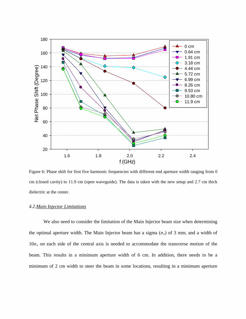
In addition to comparing phase shift of the two setups for the same aperture width, we

also need to compare the phase shift for different aperture widths for the new setup. Fig. 6 shows

the phase shift at first five harmonic frequencies of the pipe for each aperture width. For 0 cm –

3.18 cm widths, there is minimal difference in the phase shifts for each harmonic. As the

aperture width increases, phase shift at every harmonic decreases; the decrease is larger at higher

frequencies. Also, according to Equation 1, the phase shift is higher at frequencies closer to the

waveguide cut-off frequency. Therefore, we plan to use the first three harmonics to measure

phase shift since higher frequencies give smaller phase shifts.

f (GHz)1.6 1.8 2.0 2.2 2.4

Net

Pha

se S

hift

(Deg

ree)

20

40

60

80

100

120

140

160

1800 cm 0.64 cm 1.91 cm 3.18 cm 4.44 cm 5.72 cm 6.99 cm 8.26 cm 9.53 cm 10.80 cm 11.9 cm

Figure 6: Phase shift for first five harmonic frequencies with different end aperture width ranging from 0

cm (closed cavity) to 11.9 cm (open waveguide). The data is taken with the new setup and 2.7 cm thick

dielectric at the center.

4.2.Main Injector Limitations

We also need to consider the limitation of the Main Injector beam size when determining

the optimal aperture width. The Main Injector beam has a sigma (σx) of 3 mm, and a width of

10σx on each side of the central axis is needed to accommodate the transverse motion of the

beam. This results in a minimum aperture width of 6 cm. In addition, there needs to be a

minimum of 2 cm width to steer the beam in some locations, resulting in a minimum aperture

width of 8 cm. Fig. 7 illustrates the Main Injector beam size and other contributing factors to

determine the minimal aperture width necessary for beam passage.

Figure 7: Cross section of Main Injector beam pipe, illustrating the beam size and optimal aperture width.

We studied four aperture widths larger than 8 cm: 8.26 cm, 9.53 cm, 10.80 cm and 11.9

cm. Boundary conditions reduce the phase signal for 10.80 cm and 11.9 cm widths as shown in

Fig. 5. Moreover, 8.26 cm aperture width shows larger phase shift than 9.53 cm width does.

Therefore, we determined that 8.26 cm is the optimal aperture width to use for further study of

boundary conditions.

4.3.Effect of ferrite

To model an infinite beam pipe, we further adds ferrite rods at the ends of the two short

pipes to absorb the microwave signal. S21 phase shift measurement with 8.26 cm aperture width

indicates that using ferrite further enhances the phase signal. The graph in Fig. 8 represents data

taken with 2.7 cm thick dielectric at the center of the three setups: the original setup (black,

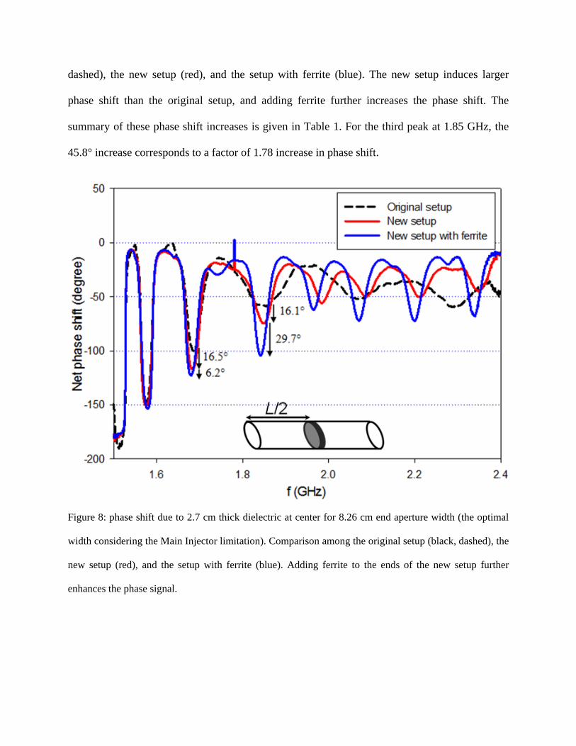
dashed), the new setup (red), and the setup with ferrite (blue). The new setup induces larger

phase shift than the original setup, and adding ferrite further increases the phase shift. The

summary of these phase shift increases is given in Table 1. For the third peak at 1.85 GHz, the

45.8° increase corresponds to a factor of 1.78 increase in phase shift.

Figure 8: phase shift due to 2.7 cm thick dielectric at center for 8.26 cm end aperture width (the optimal

width considering the Main Injector limitation). Comparison among the original setup (black, dashed), the

new setup (red), and the setup with ferrite (blue). Adding ferrite to the ends of the new setup further

enhances the phase signal.

Peak Frequency Phase increase

(new setup) Phase increase

(ferrite) Total phase

increase

Second 1.68 GHz 16.5° 6.2° 22.7° Third 1.85 GHz 16.1° 29.7° 45.8°

Table 1: Summary of phase shift increase due to the new setup and the setup with ferrite at the second and

third peaks for 2.7 cm thick dielectric at center of the setup and 8.26 cm aperture width.

We repeated the experiment by varying the position of the dielectric inside the pipe. We

placed the dielectric at one-third, one-fourth and one-fifth of the pipe length and measure the

phase shift. There is similar, but smaller, increase in phase shift for all these positions. Fig. 9

shows the phase shift for three different setups with the dielectric at one-third of the pipe length.

We see that there is a node in phase shift after every two peaks. When the dielectric is at one-

third position, the dielectric is at the node of the microwave signal every third harmonic, at

which it does not induce any phase shift. For the second to the fifth peaks, the new setup induces

about 10° - 20° larger phase shift than the original setup. Using ferrite increases the phase shift

by additional 2° - 20° at these harmonics. At the fourth peak at 1.85 GHz, the total increase for

using the setup with ferrite over the original setup is 32.5°, which amounts to 1.68 times increase

in phase shift. There are also similar increases for one-fourth and one-fifth positions of the

dielectric.

Figure 9: phase shift due to 2.7 cm thick dielectric placed at one-third of the setup with 8.26 cm aperture

width. The graph compares data for the original setup (black, dashed), the new setup (red), and the setup

with ferrite (blue).

The electron cloud will not always have a uniform density across the cross section of the

beam pipe as the Teflon dielectric does. We, therefore, need to make sure that this increase in

phase shift is not specific for the uniform density of the whole-sized dielectric. We use two half-

sized dielectrics, cut along the x and y axes (referred to as long and short half-sized dielectric

respectively) to study the effect of the dielectric spatial distribution profile. Fig. 10 shows the

phase shift when we place the 1.35 cm thick short half-sized dielectric at the center of each setup.

There is significant increase in phase shift when we use ferrite to absorb microwave. At 1.69

GHz, the setup with ferrite induces 1.47 times larger phase shift than the original setup. The

increase is more significant around 1.85 GHz where there is 2.63 times increase in phase shift for

the setup with ferrite. Even though there is significant increase in phase shift, the absolute value

of the phase shift for this half-sized dielectric is much smaller than that for the whole-sized

dielectric in Fig. 8. This smaller increase compared to the whole-sized dielectric is due to the

shape that is half as much as the whole dielectric and the 1.35 cm thickness, which is one-half

the thickness of the dielectric in Fig. 8.

Figure 10: phase shift due to 1.35 cm thick short half-sized dielectric placed at the center of the setup with

8.26 cm aperture width. The graph compares the data for the original setup (black, dashed), the new setup

(red), and the setup with ferrite (blue).

4.4.Effect of horn antenna

We also did phase shift measurement for the setup with horn antenna to couple out the

microwave signal. For this setup, we use copper tape to electrically connect horn antennas to the

ends of the two short pipes in the new setup. Fig. 11 shows the phase shift for the setup with horn

antenna compared to the original and new setups. Even though adding the two short pipes

improves phase shift, adding horn antenna to this new setup decreases the phase shift. For 8.26

cm aperture width shown in Fig. 11, the setup with horn antenna has similar phase shift signal

with the original setup. The possible reasons for this decrease may be that the boundary

condition for horn antenna is different from that of ferrite rods, and the transmission and the

reflection coefficients of the horn antenna is not ideal as it is made of aluminum.

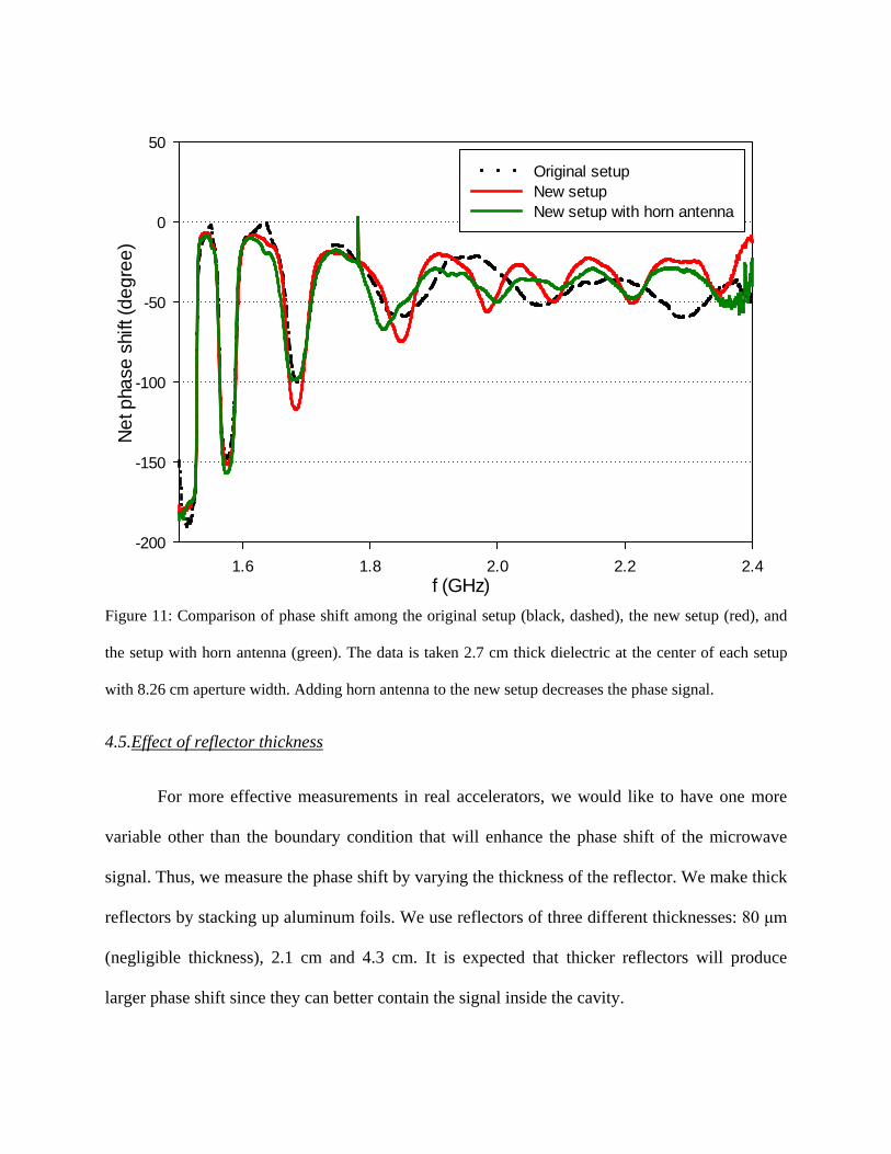
Figure 11: Comparison of phase shift among the original setup (black, dashed), the new setup (red), and

the setup with horn antenna (green). The data is taken 2.7 cm thick dielectric at the center of each setup

with 8.26 cm aperture width. Adding horn antenna to the new setup decreases the phase signal.

4.5.Effect of reflector thickness

For more effective measurements in real accelerators, we would like to have one more

variable other than the boundary condition that will enhance the phase shift of the microwave

signal. Thus, we measure the phase shift by varying the thickness of the reflector. We make thick

reflectors by stacking up aluminum foils. We use reflectors of three different thicknesses: 80 μm

(negligible thickness), 2.1 cm and 4.3 cm. It is expected that thicker reflectors will produce

larger phase shift since they can better contain the signal inside the cavity.

f (GHz)1.6 1.8 2.0 2.2 2.4

Net

pha

se s

hift

(deg

ree)

-200

-150

-100

-50

0

50

Original setupNew setupNew setup with horn antenna

We first measure the phase shift with different reflector thicknesses for the new setup.

Fig. 12 compares phase shift for the three thicknesses. In accordance with the expectation, for the

same new setup, thicker reflector induces larger phase shift. Table 2 provides the summary of

these phase shift increases for the second, third and fourth peaks. At the third peak around 1.83

GHz, the phase shift for 4.3 cm reflector thickness is 1.73 times that for the 80 μm thickness.

Peak Frequency Phase increase

(2.1 cm) Phase increase

(4.3 cm) Total phase

increase

Second 1.69 GHz 6.0° 23.7° 29.7° Third 1.83 GHz 22.1° 24.0° 46.1° Fourth 1.99 GHz 42.9° -6.4° 36.5°

Table 2: Summary of phase shift increase due to increase in reflector thickness for the new setup for 2.7

cm thick dielectric at the center of the setup and 8.26 cm aperture width.

Figure 12: phase shift due to 2.7 cm thick dielectric at the center of the new setup for 8.26 cm aperture

width. The graph compares phase shift for three different thicknesses: 80 μm (negligible thickness), 2.1

cm and 4.3 cm. The phase signal is generally larger for thicker reflector.

We repeat the measurement for the setup with ferrite at the boundary, and the data is

shown in Fig. 13. We see similar increase in phase shift for larger reflector thickness. Table 3

shows the summary of phase shift increase for the setup with ferrite at the boundary for each

reflector thickness. The most significant increase occurs at the fourth peak at 1.99 GHz, where

4.3 cm thick reflector induces 48° larger phase shift than 80 μm thickness, corresponding to 1.89

times increase in phase shift. However, phase shift increase for thicker reflectors in the setup

with ferrite at the boundary is less pronounced than that in the new setup. This is because phase

shift for thinner reflectors is larger in the setup with ferrite while that for 4.3 cm thick reflector in

both setup are approximately the same indicating that the ferrite boundary condition does not

contribute much to the phase shift.

Figure 13: phase shift due to 2.7 cm thick dielectric at the center of the setup with ferrite for 8.26 cm

aperture width. The graph compares phase shift for three different thicknesses: 80 μm (negligible

thickness), 2.1 cm and 4.3 cm. The phase signal is generally larger for thicker reflector.

Peak Frequency Phase increase

(2.1 cm) Phase increase

(4.3 cm) Total phase

increase

Second 1.69 GHz 4.5° 21.1° 25.6° Third 1.83 GHz 6.6° 4.4° 11° Fourth 1.99 GHz 45.6° 2.4° 48.0°

Table 3: Summary of phase shift increase due to increase in reflector thickness for the setup with ferrite at

boundary for 2.7 cm thick dielectric at the center of the setup and 8.26 cm aperture width.

To see this more clearly, we compare the phase shift of different setups for the same

reflector thickness. Fig. 14 shows the comparison between the two setups for 4.3 cm thick

reflector. We see that the phase shifts for the two setups are comparable for this reflector

thickness; the setup with ferrite has larger phase shift at 1.99 GHz while the new setup (without

ferrite) has larger phase shift at 1.83 GHz and 2.14 GHz. Therefore, for thick enough reflector,

ferrite is not much effective in improving the phase shift.

Figure 14: phase shift due to 2.7 cm thick dielectric at the center of the setup for 8.26 cm aperture width

and 4.3 cm reflector thickness. phase shift for the new setup (red) and the setup with ferrite (blue) are

comparable; each setup has a larger phase shift than the other at certain harmonic frequencies.

4.6.Effect of localized dielectric vs. distributed dielectric

Fig. 14 indicates that for thicker reflectors, improving boundary conditions does not

significantly enhance the phase shift. Therefore, we hypothesize that reflector thickness may be

the dominant factor in phase shift improvement. To systematically study this, we use two

different dielectrics, localized dielectric (Teflon, εr = 2.03, 2.7 cm thickness) and distributed

dielectric (Styrofoam, εr = 1.03), and measure the phase shift for 80 μm and 4.3 cm reflector

thicknesses in the original and new setups. The distributed Styrofoam dielectric is more similar

to the electron cloud than the localized Teflon dielectric does since it is spread throughout the

pipe and Styrofoam has smaller dielectric constant than Teflon. We expect to see that for the

same reflector thickness, better boundary conditions will induce larger increase in phase shift,

and vice versa. We also expect that increasing the reflector thickness (using 4.3 cm reflector and

original setup) will cause larger phase shift enhancement than improving the boundary condition

does (using reflector and new setup).

First, we measure the phase shift for the original and new setups with 80 μm and 4.3 cm

thick reflectors using distributed Styrofoam dielectric. Fig. 15 shows the plots comparing the

four measurement configurations. We see that for both 80 μm and 4.3 cm reflector thicknesses,

the phase shift for the new setup is larger than that for the original setup. Moreover, for both

setups, 4.3 cm thick reflector induces larger phase shift than 80 μm thick reflector. In addition,

we see that the phase shift for 4.3 cm thick reflector with original setup is larger than that for 80

μm thick reflector with new setup. This means that increasing the reflector thickness is a more

dominant factor in phase shift enhancement than improving the boundary conditions by adding

two pipes. The new setup with 4.3 cm reflector thickness induces the largest phase shift among

the four setups. Table 4 contains the phase shift data of this setup compared to the original setup,

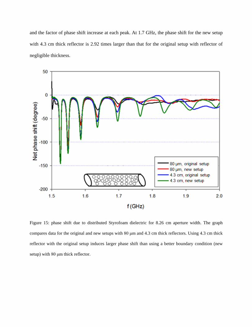
and the factor of phase shift increase at each peak. At 1.7 GHz, the phase shift for the new setup

with 4.3 cm thick reflector is 2.92 times larger than that for the original setup with reflector of

negligible thickness.

Figure 15: phase shift due to distributed Styrofoam dielectric for 8.26 cm aperture width. The graph

compares data for the original and new setups with 80 μm and 4.3 cm thick reflectors. Using 4.3 cm thick

reflector with the original setup induces larger phase shift than using a better boundary condition (new

setup) with 80 μm thick reflector.

Peak Frequency Phase (0 cm,

original setup) Phase (4.3cm,

new setup) Total phase

increase

Third 1.59 GHz 60.4° 94.8° 34.4° Fourth 1.64 GHz 31.6° 68.6° 37.0° Fifth 1.70 GHz 19.0° 55.5° 36.5

Table 4: Summary of phase shift increase due to distributed Styrofoam dielectric for the original setup

with 80 μm thick reflector and the new setup with 4.3 cm thick reflector, using 8.26 cm aperture width.

We also measure the phase shift for these four configurations using 2.7 cm thick Teflon

dielectric at the center and one-third of the setup. Fig. 16 and 17 show phase shift data for each

dielectric location. Both figures show that thicker reflector produces larger phase shift for the

same setup, and better boundary conditions induces larger phase shift for the same reflector

thickness. However, in contrast to the distributed Styrofoam dielectric, 4.3 cm thick reflector

with new setup induces a smaller phase shift than 80 μm thick reflector with original setup.

Therefore, for localized dielectric, improving the boundary conditions is a more dominant factor

in increasing the phase shift. Moreover, improving the boundary condition and adding thick

reflector enhances the phase shift significantly independent of whether the dielectric is localized

or distributed. Therefore, we conclude that a simple enhancement to the existing setup in the

Main Injector by adding thick reflectors could improve the measurement of electron cloud

density using microwave reflection technique.

Figure 16: phase shift due to localized Teflon dielectric (2.7 cm thickness) at the center of the setup for

8.26 cm aperture width. The graph compares data for the original and new setups with 80 μm and 4.3 cm

thick reflectors.

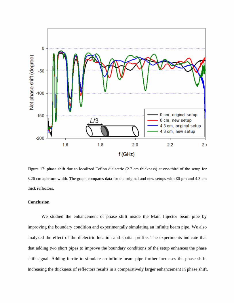
Figure 17: phase shift due to localized Teflon dielectric (2.7 cm thickness) at one-third of the setup for

8.26 cm aperture width. The graph compares data for the original and new setups with 80 μm and 4.3 cm

thick reflectors.

Conclusion

We studied the enhancement of phase shift inside the Main Injector beam pipe by

improving the boundary condition and experimentally simulating an infinite beam pipe. We also

analyzed the effect of the dielectric location and spatial profile. The experiments indicate that

that adding two short pipes to improve the boundary conditions of the setup enhances the phase

shift signal. Adding ferrite to simulate an infinite beam pipe further increases the phase shift.

Increasing the thickness of reflectors results in a comparatively larger enhancement in phase shift.

Thus, we conclude that the reflector thickness is the major factor in phase shift improvement and

for thick enough reflectors, improving the boundary conditions do not have significant effect on

overall phase shift. Experimental studies with distributed dielectric also proved this hypothesis

that reflector thickness rather than the boundary condition is the dominant factor in enhancing

the phase shift. Therefore, to measure the electron cloud density that is distributed inside the

beam pipe using microwave technique, adding thick reflectors will increase the phase shift of the

microwave signal. Further microwave and particle simulations are being done to study the effect

of actual proton bunch on electron cloud [11].

Acknowledgement

We thank Bob Zwaska, Young Min Shin, Cheng-Yang Tan, and Nathan Eddy for

contributing thoughts on possible improvements of the setup. We also thank Brian Fellenz for

providing the equipments and other assistance. One of the authors (J. T.) would also like to thank

John Sikora for his discussion and encouragement of this measurement.

References

[1] I. Kourbanis, P. Adamson, B. Brown, D. Capista, W. Chou, D. Morris, K. Seyia, G. Wu, M.J.

Yang, “Current and Future High Power operation of Fermilab Main Injector”, Fermilab Note,

fermilab-conf-09-151-1d

[2] K.G. Sonnad, M. Furman, S. Veitzer, P. Stoltz, J. Cary, “Simulation and Analysis of

Microwave transmission through an electron cloud, a comparison of results”, Proceedings of

PAC’07

[3] T. Kroyer, F. Caspers, E. Mahner, T. Wien, “The CERN SPS experiment on microwave

transmission through the beam pipe”, Proceedings of PAC’05

[4] S. De Santis, J.M. Byrd, F. Caspers, A. Krasnykh, T. Kroyer, M.T.F. Pivi, K.G.Sonnad,

“Measurment of Electron Clouds in Large Accelerators by Microwave Dispersion”, Phys.

Rev. Lett 100, 094801 (2008)

[5] J.P. Sikora, R.M. Schwartz, M.G. Billing, D.L. Rubin, D. Alesini, B.T. Carlson, K.C.

Hammond, S. De Santis, “Using TE Wave Resonances for the Measurement of Electron

Cloud Density”, IPAC’12, New Orleans, LA, MOPPR074

[6] G. Rumolo, G. Arduini, E. M’etral, E. Shaposhnikova, E. Benedetto, G. Papotti, R. Calaga, B.

Salvant, “Experimental Study of the Electron Cloud Instability at the CERN-SPS”, EPAC’08,

Genoa, Italy, pp TUPP065, June 2008

[7] J.C. Thangaraj, N. Eddy, B. Zwaska, J. Crisp, I. Kourbanis, K. Seiya, “Electron Cloud

Studies in the Fermilab Main Injector using Microwave Transmission”, ECLOUD 2010,

Ithaca, New York; USA

[8] K.G. Sonnad, F. Caspers, I. Birkel, S. Casalbuoni, E. Huttel, D.S. de Jauregui, A. Muller, R.

Wiegal, “Observation of Electron Clouds in the ANKA Undulator by means of the

Microwave Transmission Method”, PAC’09, Vancouver, BC, Canada, TH5RFP044

[9] C.Y. Tan, “Measuring electron cloud density with trapped modes”, Fermilab Note

(unpublished)

[10]H. Wang, J.C. Thangaraj, B. Zwaska, C.Y. Tan, B.J. Fellenz, “Microwave reflection

technique for electron cloud density measurement”, Fermilab Lee Teng intern 2011 note

(unpublished);

http://www.illinoisacceleratorinstitute.org/2011%20Program/student_papers/Hexuan_Wang.

pdf

[11] Y.M. Shin, J.C. Thangaraj, C.Y. Tan, B. Zwaska, “Electron Cloud Density Analysis using

Microwave Cavity Resonance”, 2012, Pending publication