
Driven Eigenproblem Computation for Periodic Structures · PDF fileDriven Eigenproblem...
124
Technische Universit¨ at M¨ unchen Lehrstuhl f¨ ur Hochfrequenztechnik Driven Eigenproblem Computation for Periodic Structures Huanlei Chen Vollst¨ andiger Abdruck der von der Fakult¨ at f¨ ur Elektrotechnik und Informationstechnik der Technischen Universit¨ at M¨ unchen zur Erlangung des akademischen Grades eines - Doktor-Ingenieurs - genehmigen Dissertation Vorsitzender : Univ.-Prof. Dr.-Ing. Eckehard Steinbach Pr¨ ufer der Dissertation : 1. Univ.-Prof. Dr.-Ing. Thomas Eibert 2. Prof. Dr. Wenquan Che, Nanjing University of Science and Technology/China Die Dissertation wurde am 15.04.2013 bei der Technischen Universit¨ at M¨ unchen eingereicht und durch die Fakult¨ at f¨ ur Elektrotechnik und Informationstechnik am 30.09.2013 angenommen.
Transcript of Driven Eigenproblem Computation for Periodic Structures · PDF fileDriven Eigenproblem...

Technische Universitat Munchen
Lehrstuhl fur Hochfrequenztechnik
Driven Eigenproblem Computation for
Periodic Structures
Huanlei Chen
Vollstandiger Abdruck der von der Fakultat fur Elektrotechnik und Informationstechnikder Technischen Universitat Munchen zur Erlangung des akademischen Grades eines
- Doktor-Ingenieurs -
genehmigen Dissertation
Vorsitzender : Univ.-Prof. Dr.-Ing. Eckehard Steinbach
Prufer der Dissertation : 1. Univ.-Prof. Dr.-Ing. Thomas Eibert2. Prof. Dr. Wenquan Che,
Nanjing University of Science and Technology/China
Die Dissertation wurde am 15.04.2013 bei der Technischen Universitat Muncheneingereicht und durch die Fakultat fur Elektrotechnik und Informationstechnikam 30.09.2013 angenommen.


Contents
Acknowledgement 5
Abbreviations and Symbols 7
1 Abstract 1
2 Introduction 3
2.1 Background . . . . . . . . . . . . . . . . . . . . . . . . . . . . . . . . . . . 32.2 Motivation . . . . . . . . . . . . . . . . . . . . . . . . . . . . . . . . . . . . 42.3 Focus of this Work . . . . . . . . . . . . . . . . . . . . . . . . . . . . . . . 52.4 Organization . . . . . . . . . . . . . . . . . . . . . . . . . . . . . . . . . . 6
3 Metamaterials and SIWs 9
3.1 Metamaterials . . . . . . . . . . . . . . . . . . . . . . . . . . . . . . . . . . 93.1.1 Fundamentals of Metamaterials . . . . . . . . . . . . . . . . . . . . 93.1.2 Modeling and Realization of Metamaterials . . . . . . . . . . . . . 10
3.2 Substrate Integrated Waveguide (SIW) . . . . . . . . . . . . . . . . . . . . 153.2.1 Characteristics of SIWs . . . . . . . . . . . . . . . . . . . . . . . . 163.2.2 Dierent Types of SIWs . . . . . . . . . . . . . . . . . . . . . . . . 173.2.3 Existing Modeling Methods for SIWs . . . . . . . . . . . . . . . . . 193.2.4 Limitations of Existing Methods . . . . . . . . . . . . . . . . . . . 20
4 Modeling of Periodic Congurations 23
4.1 Eigenproblem Formulation for Electromagnetic Fields . . . . . . . . . . . 234.1.1 Maxwell's Equations . . . . . . . . . . . . . . . . . . . . . . . . . . 234.1.2 Helmholtz' Equations . . . . . . . . . . . . . . . . . . . . . . . . . 244.1.3 Floquet's Theorem . . . . . . . . . . . . . . . . . . . . . . . . . . . 254.1.4 Eigenmodes and Eigenvalues . . . . . . . . . . . . . . . . . . . . . 25
4.2 Modal Series Expansion Method . . . . . . . . . . . . . . . . . . . . . . . 264.3 Modal Expansion for Open Structures . . . . . . . . . . . . . . . . . . . . 304.4 Eigenproblem Solution with External Excitations . . . . . . . . . . . . . . 334.5 Dispersion and Modes . . . . . . . . . . . . . . . . . . . . . . . . . . . . . 34
5 Driven Eigenproblem Computation 43
5.1 Fundamentals of Driven Eigenproblem Computation . . . . . . . . . . . . 435.1.1 Analogy between Eigenproblem and Resonator . . . . . . . . . . . 435.1.2 Resonator and Excitation Setup . . . . . . . . . . . . . . . . . . . . 45
3

Contents
5.2 Port Excitation and the Perturbation Method in Small Attenuation Scenarios 455.3 Current Excitation and Implementation in FEBI . . . . . . . . . . . . . . 48
5.3.1 Fundamentals of FEBI . . . . . . . . . . . . . . . . . . . . . . . . . 485.3.2 Implementation of the Driven Method in FEBI . . . . . . . . . . . 50
5.4 Complex Waves . . . . . . . . . . . . . . . . . . . . . . . . . . . . . . . . . 52
6 Eigenvalue Searching Acceleration in Driven Eigenproblem Computation 57
6.1 Equivalence Between Eigenvalue Searching and Maximization . . . . . . . 576.2 Brent's Method in One Direction Searching . . . . . . . . . . . . . . . . . 576.3 Powell's Quadratically Convergent Method in Multi-direction Searching . 586.4 Global Optimization for Multi-mode Scenario . . . . . . . . . . . . . . . . 60
7 Mode Selection 67
7.1 Mode Excitation . . . . . . . . . . . . . . . . . . . . . . . . . . . . . . . . 677.1.1 External Excitation of Cavity Resonator . . . . . . . . . . . . . . . 677.1.2 Internal Excitation of Cavity Resonator . . . . . . . . . . . . . . . 68
7.2 Mode Distinction . . . . . . . . . . . . . . . . . . . . . . . . . . . . . . . . 69
8 Applications 71
8.1 Classical Rectangular Waveguide: A Verication Example for Small At-tenuation Scenarios . . . . . . . . . . . . . . . . . . . . . . . . . . . . . . . 71
8.2 Substrate Integrated Waveguide (SIW): Small Radiation Example . . . . . 748.3 CRLH Leaky Wave Antenna: Interdigital Design Analysis . . . . . . . . . 778.4 Periodic Modulated Grounded Dielectric Corrugated Leaky Wave An-
tenna: Multi-mode Analysis . . . . . . . . . . . . . . . . . . . . . . . . . . 808.4.1 Model in 1D Periodic . . . . . . . . . . . . . . . . . . . . . . . . . . 808.4.2 1D Periodic Model with Finite Width . . . . . . . . . . . . . . . . 86
8.5 Mushroom Structure for MTM: 2D Periodic Conguration . . . . . . . . . 91
9 Conclusions 97
10 Appendix 99
10.1 General Properties of the Eigenfunctions . . . . . . . . . . . . . . . . . . . 9910.2 General Matrix System for CRLH 2D Networks . . . . . . . . . . . . . . . 10110.3 Periodic Green's Function . . . . . . . . . . . . . . . . . . . . . . . . . . . 104
List of Figures 106
4

Acknowledgement
I would like to thank Prof. Dr.-Ing. Thomas Eibert for giving me the opportunities tostudy in the Lehrstuhl für Hochfrequenztechnik, Technische Universität München, Mu-nich, Germany. His motivation and advice inspired me in both study and life. I also mustsay thanks to the International Graduate School of Science and Engineering (IGSSE) ofTUM for sponsoring me through my study and every conference. The help from the col-laborative Nanjing University of Science and Technology, Department of CommunicationEngineering, Nanjing, especially Prof. Wenquan Che and the other colleagues Wenjie,Yumei and so on are unforgettable. Without them my international exchange can no beso successful. I am specially grateful to Dr.-Ing. Carsten Schmidt and Prof. Dr.-Ing. UweSiart for their valuable supports. Moreover I would like to dedicate this work to myfamily. My parents in China always give me the courage to complete this work. Myhusband Libo Huang stands beside me and plays all kinds of roles like adviser, reviewerand critic. His help is the solid foundation in the successful completion of my studies.Finally I would like to thank my upcoming baby for his cooperation during the thesiswriting. Although being exhausted and encountering a big change of life, I still deeplyappreciate the happiness he brings.
5


Abbreviations and Symbols
ABC absorbing boundary conditionABCD-matrix transmission matrix with respect to voltage and currentB magnetic ux densityC capacitorCRLH composite right-/left-handedBI-RME boundary integral-resonant mode expansion methodD electric displacement vectorE electric eldEC evolutionary computationEM eigenmodeES evolution strategyEV eigenvalueFDFD nite dierence frequency domainFDTD nite dierence time domainFEBI nite element boundary integralFEM nite element methodFSIW folded substrate integrated waveguideGO geometrical opticsGP genetic programmingGTD geometrical theory of diractionH magnetic eld vectorHMSIW half mode substrate integrated waveguidek′′ attenuation constantk′ phase constantε0 8.858 · 10−12 F/m, permittivity of free spaceεr relative permittivityk wavenumberk wavevectorL inductorLH left handLHMs left-handed materialsLTCC low temperature co-red ceramicMFS method of fundamental solutionsMCMC Markov chain Monte CarloMoL method of lines
7

Abbreviations and Symbols
MoM method of momentsMTM metamaterialMP matrix-pencilMW magnetic wallλ wavelengthλg guided wavelengthλ0 wavelength in free spaceLCS learning classier systemµ0 4π · 10−7 Vs/(Am), permeability of free spaceµr relative permeability∇ Nabla operator, gradient∇· divergence operator∇× curl operatorPBC periodic boundary conditionPCB printed circuit boardPEC perfect electric conductorPMC perfect magnetic conductorPML perfectly matched layerPO physical opticsPTD physical theory of diractionRH right handRO random optimizationRSIW ridged substrate integrated waveguideSA simulated annealingS-matrix scattering matrixSIW substrate integrated waveguideSMA scattering matrix approachSRR split-ring resonatorSTUN stochastic tunnelingtan δ loss factorTEM transverse electromagnetic waveTL transmission lineTrL the numerical thru-line calibration methodTW thin-wire4 = ∇2 Laplace operatorvp phase velocityvg group velocityω0m magnetic resonant frequencyωpe electric plasma frequencyωpm magnetic plasma frequencyωse series resonant frequencyωsh shunt resonant frequency
8

1 Abstract
With increasing operating frequencies, new microwave structures with the advantages oflow loss and high quality factor for microwave, millimeter wave or even terahertz frequen-cies have come into research focus. One promising structure is the substrate integratedwaveguide (SIW) which constructs the traditional hollow waveguide in a planar printedcircuit board (PCB) with the characteristics of high density integration ability, low cost,low losses and high quality factor. One of the other research tendencies is to create a newkind of materials with negative permittivity and permeability simultaneously which arecalled metamaterials. These two new technologies both employ periodic congurationswhich normally have ne details, large size, open geometry and induce big diculties inmodeling the electromagnetic elds inside and outside the structures. Principally anyelectromagnetic eld problem in source free region can be treated as an eigenproblemwithout excitation. The eigenproblem in a periodic structure normally requires morediscretization due to the complicated conguration which leads to a considerable numberof unknowns. Therefore, the eigenproblem in a periodic structure is usually compli-cated and even nonlinear. The existing modeling method for metamaterials based on thecomposite right-/left-handed transmission line theory restrains its application to certaintypes of waves, normally TEM modes, by purely describing the circuit with voltage andcurrent. Some other numerical methods based on the classical eigenvalue solvers with theaid of the method of moments or FDTD may face the problem of bad convergence espe-cially for the large size of the numerical systems which are induced by periodic structures.
This work proposes a novel driven eigenproblem computation method to solve theeigenproblem in periodic structures. Comparing with the purely mathematical eigen-problem solvers, the driven method is to solve the periodic eigenproblem by solving thecorresponding excitation problem in the domain of the eigenvalue. For large numeri-cal systems, solving the corresponding driven problems is normally less demanding thansolving directly the eigenproblems. On the other hand according to Floquet's theoremthe wave propagation in a periodic structure can be solved inside one unit cell with thedened periodic boundary conditions. The analogy between the eigenproblem and theresonator makes it possible to analogize the eigenproblem of the unit cell of the periodicstructure to the one of a resonator whose eigenvalues are the resonance frequencies. Thesame as the resonator in electrical circuits, an internal or external excitation can be ap-plied to the unit cell and a norm of the solution like the electric eld dependent on thevarying eigenvalue is observed. The driven method is employed for the dispersion andattenuation analysis of periodic waveguiding congurations.
Dierent types of excitations to the equivalent resonator are available, one is by us-
1

1 Abstract
ing ports and the other is by distributed current densities. The port excitations canbe appropriately coupled to the eld of the equivalent resonator which analogizes theunit cell. Circuit theory can be used to regularize the eld and calculate the energytransmission and the losses in the equivalent resonator. On the other hand distributedcurrent densities, for example impressed volume current densities with dierent distri-butions or polarizations have the advantage of the specic mode selection as well asthe all-mode excitation. Corresponding to the dierent types of excitations, the drivenmethod is implemented in two solvers, respectively. One is the commercial numericalsolver CST Microwave Studio (CST MWS) and the other is the hybrid nite element-boundary integral-solver (FEBI). The implementation in CST Microwave Studio withlimited boundary exibility works well in small attenuation scenarios where the per-turbation technique is employed for the loss analysis of the propagating wave. On thecontrary the implementation in FEBI with the doubly periodic setting is more robustfor the one- or two-dimensional articial material compositions like metamaterials andsuitable for both small and large attenuation scenarios. FEBI works with an edge-basedperiodic boundary condition (PBC) based on FEM interior to the boundary. Exteriorto the boundary a surface integral equation formulation with a Floquet mode based pe-riodic Green's function is applied to fully account for the radiation and scattering ofopen structures. Lossy materials can be directly considered by supporting the complexwavevector within the periodic boundary conditions and the Green's functions.
In the driven resonator model, the resonance is always accompanied with an extremumof some electromagnetic observables, e.g. the electrical eld. This makes the search ofthe eigenvalue, which is the resonance frequency in the resonator model, equivalent toa maximization process. Since the wavevector is complex in the lossy system, the max-imization will be on the complex plane of the wavevector which actually leads to amulti-dimensional maximization. With the start vector estimation based on the previoussolutions, the driven method requires the repeated iterations of solutions of excitationproblems with slightly varying parameters. Some optimization techniques are employedto achieve fast convergence in one or more dimensional searching. After providing thetheoretical background, a series of application examples are presented. First, the dis-persion behavior of a classical rectangular hollow waveguide is analyzed by the drivenmethod and compared with the analytical results stated in the literature to verify thedriven method. Then one SIW with uniform cross section in wave propagation directionand small radiation loss is modeled in a unit cell with the driven method and the disper-sion and attenuation curves match to the results from a longer model with the same unitcell congurations in CST MWS. Next a composite right-/left-handed (CRLH) waveg-uide, which is implemented by the SIW technology, is also modeled by the driven methodwith port excitations. Comparing with other modeling methods like the scattering ma-trix approach or the matrix pencil technique, the driven method can generate accurateresults in the dispersion analysis. The examples of a grounded dielectric corrugated leakywave antenna (LWA) and a metamaterial based on the so-called mushroom structure ex-hibit the versatility of the driven method in analysis of 1- and 2- dimensional periodicstructures and multi-mode operations.
2

2 Introduction
2.1 Background
Microwave devices and components are playing a more and more important role in mod-ern communication, remote sensing, automotive industry and bioelectromagnetic applica-tions. But the increasingly sophisticated designs, the complex structures and the higheroperating frequency range on the other hand make the modeling of the electromagneticeld inside and outside the components a big challenge. Basically all the electromag-netic problems can be represented in Maxwell's equations of the dierential or integralforms with the corresponding boundary conditions to nd the solution. Unfortunately,Maxwell's equations can be solved analytically only for a very few idealized geometries.However, thanks to the development of the computer technology, the accurate and com-plete analysis of complex microwave structures can be achieved by solving Maxwell'sequations numerically. Maxwell's equations can be considered as eigenproblems, whoseeigenvalues and eigenvectors suciently characterize the system under analysis. Thereare a variety of numerical methods for solving the eigenproblem of electromagnetics ineither the time domain or the frequency domain. Time-domain methods model the tran-sient behavior of the eld and solve simultaneously many frequencies. Frequency-domainmethods solve one frequency at a time. The solutions in the two domains can be trans-formed to each other by the Fourier transforms.
The three fundamental numerical methods which are the nite dierences, the niteelements, and the moment methods have a long history and are well developed. The mostwidely used methods are the nite-dierence time-domain (FDTD) method [Yee, 1966],the nite element method (FEM) [Cesari & Abel, 1972], the method of moments (MoM)solution of integral equation formulations [Harrington, 1968], the high-frequency meth-ods like the geometrical optics (GO) [Schuster, 1904], [Greivenkamp, 2004], the physi-cal optics (PO) [Akhmanov & Nikitin, 1997], [Asvestas, 1980], the geometrical theory ofdiraction (GTD) [Keller, 1962], the physical theory of diraction (PTD)[Umtsev, 2007], as well as hybrid methods which combine the dierent methods to-gether, e.g. the hybrid nite-element boundary-integral method (FEBI)[Eibert et al., 1999] and so on. However, almost all of the numerical methods followcertain steps to model the problems. They all begin with discretizing the continuous un-known quantities like elds or currents in spatial or temporal domains into a computer-handleable set of nite quantities. Normally the ner the discretization is, the moreaccurate the result can be, but at the same time the more memory of the computerand the heavier computation load are needed. The electromagnetic quantities can beapproximated by a set of expansion functions which transform the eigenproblems into a
3
2 Introduction
linear algebraic equation system. These algebraic equations are solved to determine theunknown coecients of the expansion functions and nally the electromagnetic elds orcurrents can be interpreted. The dierent methods employ variant strategies to solvethe unknown coecients, for example the inversion of large matrices, implicit and ex-plicit iteration schemes, evolutionary algorithms, random walks and the combinationsof them. Although the numerical solvers have been developed for a long time, they arestill facing diculties in solving the eigenproblems for large numerical system, e.g. un-satised convergence for periodic structures. Many electromagnetic eld problems caneven evoke nonlinear eigenproblems which are even more challenging to solve. Therefore,many eigenproblem computations are restricted to small problem size like the dispersionanalysis of waveguides where only one- or two-dimensional problems are needed to besolved.
2.2 Motivation
In recent researches, periodic structures attract more and more interest. In 1968, asubstance with the character of "simultaneously negative permittivity ε and perme-ability µ", so called the left-handed (LH) eect, was rstly theoretically speculated in[Veselago, 1968]. The substance was named metamaterial whose name itself stands forarticially structured materials while none of them has been found in nature until now.In 2000, the rst experimental demonstrator of a metamaterial with negative ε and µ in acertain frequency range was proposed in [Smith et al., 2000]. Small inhomogeneous com-ponents like thin-wires and split-ring resonators, whose average sizes are much smallerthan the guided wavelength, create an eective macroscopic homogeneous behavior. How-ever, the lossy and narrow band characteristics make this kind of designed compositionnot a good solution for realistic applications. After that an engineering approach of de-signing metamaterials by using the well-known lumped-element equivalent circuit modelwas developed. The composite right/left-handed transmission line (CRLH TL) methodrealized the left-handed eect in a certain frequency range together with the naturalright-handed lumped or distributed circuit elements [Caloz & Itoh, 2002], [Oliner, 2003],[IYER & Eleftheriades, 2002]. The LH eect makes metamaterials a good choice for an-tennas, frequency selective surfaces, absorber materials, superlens, and cloaking devicesand many other applications. The majority of up-to-date conceived CRLH TL con-gurations are based on microstrip line designs and sometimes on substrate integratedwaveguides (SIWs), especially at millimeter and terahertz frequencies. SIW is a hybridtechnology which emulates a dielectric lled hollow waveguide in a planar structure,e.g. a printed circuit board (PCB), by replacing the vertical side walls of the waveguidewith lateral rows of vias [Bozzi et al., 2009]. The quasi closed conguration gives SIWsa better power handling capacity compared to microstrip lines. Also the planar congu-ration makes SIWs easily compatible to other integrated circuits. However, in the highfrequency range the radiation losses due to the periodic lateral openings in SIWs cannot be omitted. Both metamaterials and SIWs employ periodic congurations. Conse-quently the large scale, the ne details and the unclosed geometry of the metamaterials
4

2.3 Focus of this Work
and SIWs make their modeling complicated complex eigenproblems. The existing circuit-based modeling method like CRLH TL for metamaterials describes the structures underanalysis with voltages and currents restrained to some certain waves, e.g. the TEM mode,and is not sucient for modeling of arbitrary waveguiding structures with sometimes in-homogeneous material lling and multi-mode operation. On the other hand, periodicstructures like metamaterials and the SIWs with two- or even three-dimensional periodiccongurations will evoke eigenproblems with a considerably large number of unknowns.This places big challenges for the classical numerical eigenproblem-based methods. Theclassical eigenproblem solvers which try to solve directly the eigenproblem from a math-ematical point of view, can always nd dicult convergence and bad accuracy especiallyin large and often open eigenproblem systems as found for periodic structures.
2.3 Focus of this Work
The popularity of periodic structures and their modeling diculties motivate us to ndan ecient way to solve the eigenproblems of periodic structures. This work investigatesa novel driven eigenproblem computation method to solve the eigenproblem of periodicmicrowave structures. Compared to the purely mathematical eigenproblem solvers, thedriven method solves the periodic eigenproblem by solving the corresponding excita-tion problem in the domain of the eigenvalue with less computation eort than directlysolving the source-free eigenproblem. The analogy between the eigenproblem and theresonator opens up an opportunity to transfer the eigenproblem into a resonator wherethe eigenvalues are the resonance frequencies. According to the Floquet's theorem theperiodic structure can be analyzed in one unit cell with periodic boundary conditionswhich greatly reduces the problem domain and computation eorts. Similar as for aresonator in electrical circuits, an internal or external excitation can be applied to theequivalent resonator which analogizes to the eigenproblem under consideration and anorm of the solution dependent on the varying eigenvalues is observed to nd out theresonance frequencies.
Dierent types of excitations are available for the equivalent resonator. External exci-tations like port excitations can be designed to well couple to the eld of the equivalentresonator which can be transformed to an equivalent circuit. Microwave network theoryas e.g. in form of the scattering matrix can then be used to analyze the eld problem. Theinternal excitations like the distributed volume current densities inside the solution do-main with dierent distributions or polarizations can stimulate one certain mode as wellas all the relevant modes. Dierent excitation methods can be implemented in dierentsolvers. The port excitation is implemented in CST Microwave Studio [CST, 2011] withinthe frequency domain solver. However, the limited periodic boundary condition exibil-ity restricts this implementation to small-attenuation scenarios where the perturbationmethod is employed to analyze the power loss in the structures. On the contrary, the dis-tributed current density excitation which is implemented with the hybrid nite-elementboundary-integral solver (FEBI) [Eibert et al., 1999] can model the doubly periodic con-
5

2 Introduction
gurations and take the attenuation directly into account by supporting the complexwavevector in the boundary conditions. Therefore, the implementation in FEBI is morerobust for one- or two-dimensional articial material compositions like metamaterialsand can work for both small and large attenuation scenarios. The driven method worksrobustly in the dispersion and attenuation analysis of periodic structures and can providephysical insight into the structure as well.
Searching the eigenvalues for the unit cell of periodic structures can be analogizedto search the resonance frequencies in resonators. In resonators, one ecient way to ndresonance frequencies is to stimulate the structure and make it resonance. In periodicstructures by providing an excitation to the unit cell which is analogized to a resonatorand monitoring the stimulated resonance can simplify the eigenvalue searching proce-dure to a maximization procedure, because the resonance is always accompanied withan extremum of the electromagnetic eld observables, e.g. the electric eld. The drivenmethod starts with a vector estimation based on the previous solutions and repeats theiterations of solutions of excitation problems for slightly varying parameters. There aretwo possibilities to search the eigenvalues, which in the periodic structure are the pairsof (resonance frequency ω, wavevector k). One is to x the wavevector k and sweep thefrequency ω till an extremum of the eld observables is found. The other is to makeω constant and vary k to locate the extremum. When the structure is lossy or doublyperiodic, k will be complex and a vector quantity. This will make the maximizationa multi-dimensional searching procedure. Many optimization techniques are employedto achieve fast convergence in one or more dimensional searching. The implementedBrent's method provides the iteration of maximization in the driven method a parabolicconvergence without calculating the divergence. The Powell's method is employed to per-form the multi-dimension maximum searching eciently. For the multi-mode operatedone- or two-dimensional periodic structures, the global optimization has been introducedto search all the local maxima which are corresponding to the dierent modes in theoperation frequency range.
2.4 Organization
In this work, after the introduction of periodic structures, like metamaterials and SIWs, abrief review of the periodic problem formulation will be given. According to the Floquet'stheorem, the periodic structure can be modeled as one appropriately discretized unit cellwith periodic boundary conditions. In chapter 4 the fundamentals of the numerical meth-ods which are employed to analyze periodic structures, like the mode expansion method,and the scattering matrix method will be introduced. For open structures, which arethe main focus of this work, absorbing layers will be introduced to enclose the analysisregion for the mode expansion method to avoid the integral formulation for the radiationof open structures. Also the characteristics of the dierent methods will be compared.This work concentrates on the dispersion analysis of periodic structures. Therefore, thefundamentals of the modes and mode dispersion are introduced.
6

2.4 Organization
In chapter 5, the analogy between the eigenproblem and the resonator is discussed.This analogy opens up a possibility to convert the eigenproblem in the periodic structureto an excitation problem in the resonator model where the resonance frequencies are theeigenvalues. In the resonator, the resonance frequencies can be easily found by applyingan excitation and monitoring the electromagnetic eld observables which will reach anextremum at the resonance frequency. This procedure can not only provide insight intothe modeling structure, but also analyze the dispersion and attenuation behavior of theperiodic structures. Dierent excitation methods, e.g. port excitations and distributedcurrent densities excitation are introduced. In section 5.1 the driven eigenproblem com-putation is realized with the commercial numerical solver CST Microwave Studio wherethe port excitations are employed. However, the limited boundary condition exibilityrestrains its application to small attenuation scenarios where the perturbation method isemployed to calculate the power loss for the guiding wave. Consequently the approachis unable to calculate the attenuation inside the stop band. Therefore, in section 5.2the driven eigenproblem approach with distributed current densities excitation is imple-mented within the periodic hybrid nite-element boundary-integral (FEBI) method withthe innite periodic multilayer Green's function. With the distributed current densitiesexcitation, one certain mode as well as all the relevant modes can be stimulated. Theimplementation in FEBI can directly support complex wavevectors within the periodicboundary conditions and the Green's function. Therefore, complex phase shifts on theperiodic boundaries are possible which means the leaky and evanescent modes can bedescribed and the attenuation inside the stop band can also be computed.
The eigenvalue, pairs of (frequency, wavevector) can fully characterize the proper-ties of a microwave system, like waveguide, resonator and so on. In the resonator theeigenvalue is the resonance frequency where an extremum of the electromagnetic eldinside the resonator will always take place. For a periodic structure, nding the reso-nance frequency in the equivalent resonator model which analogizes to the unit cell of theperiodic structure can be transformed to a maximization problem of the electromagneticeld at a specied position inside the resonator over the complex wavevector and the fre-quency. Chapter 6 describes in detail the analogy between the eigenvalue searching andthe maximization. Some acceleration methods, e.g. the Brent's and the Powell's methodare introduced to accelerate the maximization in one- and multi-dimension. In order tond out all the extrema which stand for all the resonance modes, a global optimizationneed to be employed. The frequently used methods of global optimization are introduced.
In some frequency range, more than one resonance mode can be stimulated. Chapter7 describes how to excite all modes or one specic mode by dening the current densityexcitations and how to distinguish dierent modes through comparing the electromag-netic eld distribution. In chapter 8 several application examples of the driven methodare given. A classical rectangular waveguide is analyzed by the driven method and com-pared to the analytical results stated in literature to verify the driven method. Then oneSIW structure with uniform cross section in wave propagation direction is modeled in a
7

2 Introduction
unit cell with the driven method to demonstrate the performance of the driven methodin the small attenuation scenario. The dispersion and attenuation behaviors obtainedby the driven method match to the results from a longer model with the same unit cellconguration. An interdigital CRLH waveguide which is implemented by the SIW tech-nology is also modeled in the unit cell with the driven method for the small attenuationscenario. Compared to other modeling methods like the scattering matrix approach, thedriven method can generate more accurate results in dispersion and attenuation analysis.A grounded dielectric corrugated leaky wave antenna (LWA) with dierent width andin one-dimensional periodic conguration and a metamaterial based on the mushroomstructure in two-dimensional periodic conguration are analyzed to demonstrate the ver-satility of the driven method with FEBI implementation. The acceleration methods areimplemented to speed up the convergence of the maximization.
8

3 Metamaterials and SIWs
In recent researches, periodic structures like substrate integrated waveguides and meta-materials attract more and more attention with the properties of high-density integrationpossibility or negative refractive index. However, the large scale, the ne details and theoften unclosed geometry of periodic structures make their modeling a complicated com-plex eigenproblem.
3.1 Metamaterials
3.1.1 Fundamentals of Metamaterials
Microwave metamaterials (MTMs) refer to a class of articial materials that have simul-taneously negative permittivity (ε) and permeability (µ) and sometimes they are namedleft-handed materials (LHMs). The theory of MTMs was rstly proposed by Victor Vese-lago in 1968 [Veselago, 1968]. The permittivity (ε) and permeability (µ) characterize theelectric and magnetic properties of materials interacting with electromagnetic elds. Thepermittivity is the ability of the material to store electrical energy when an electric eldis applied. It is dened as the ratio of the electric displacement vector of the medium Dand the electric eld E,D = εE. In the scientic work the relative permittivity εr, whichis the ratio of the permittivity of the material to that of free space (ε0 = 8.858 · 10−12
F/m), is commonly used. The permeability of a material indicates the relation betweenmagnetic ux density vector B and the magnetic eld vector H, B = µH. Similar toεr, µr = µ/µ0, where µ0 = 4π · 10−7 Vs/(Am). Figure 3.1 categorizes the materials by εand µ. Metamaterials were predicted to be characterized with
• necessary frequency dispersion of ε and µ,
• reversal of the Doppler eect,
• reversal of the Vavilov-Cerenkov radiation,
• reversal of the boundary conditions relating the normal components of the electricand magnetic elds at the interface between the conventional/right-handed (RH)medium and a LH medium,
• reversal of Snell's law,
• subsequent negative refraction at the interface between a RH medium and a LHmedium,
• Plasmonic expressions of ε and µ in resonant-type LH media [Veselago, 1968].
9

3 Metamaterials and SIWs
However, this kind of materials with simultaneously negative ε and µ has not been foundin nature until now.
ε
μ
ε μ< , >0 0
plasma and finewire structures
no wave propagation
ε μ< , <0 0
metamaterial
backward propagation
ε μ> , >0 0
conventional material
forward propagation
ε μ> , <0 0
microstructuredmagnets and split rings
no wave propagation
Air
Air
Air
Air
Figure 3.1: The diagram classies materials in terms of their permittivity ε and perme-ability µ. The behavior of a wave incident on the air-material interface foreach of the possible four cases is shown. The top right quadrant is a conven-tional dielectric material with positive ε and µ, which shows the refractionwith the refraction angle smaller than the incident angle. The metamaterialsin the bottom left quadrant with simultaneously negative ε and µ refract tothe same side of the normal indicating reverse Snell's law. Plasmas with neg-ative ε and positive µ and microstructured magnetic materials in the bottomright quadrant with positive ε and negative µ reect the incident wave.
3.1.2 Modeling and Realization of Metamaterials
In 2000, the rst demonstration of metamaterials was realized experimentally by Smithet al. [Smith et al., 2000]. The material was a combination of a thin-wire (TW) withnegative-ε and positive-µ and a split-ring resonator (SRR) structure with positive-ε andnegative-µ to have simultaneously negative ε and µ at certain frequencies. The averagecell size p of the combination was much smaller than the guided wavelength λg (p λg)which led to a quasi-homogeneous structure. Fig. 3.2 demonstrates the geometry of therst eectively homogeneous MTM.
10
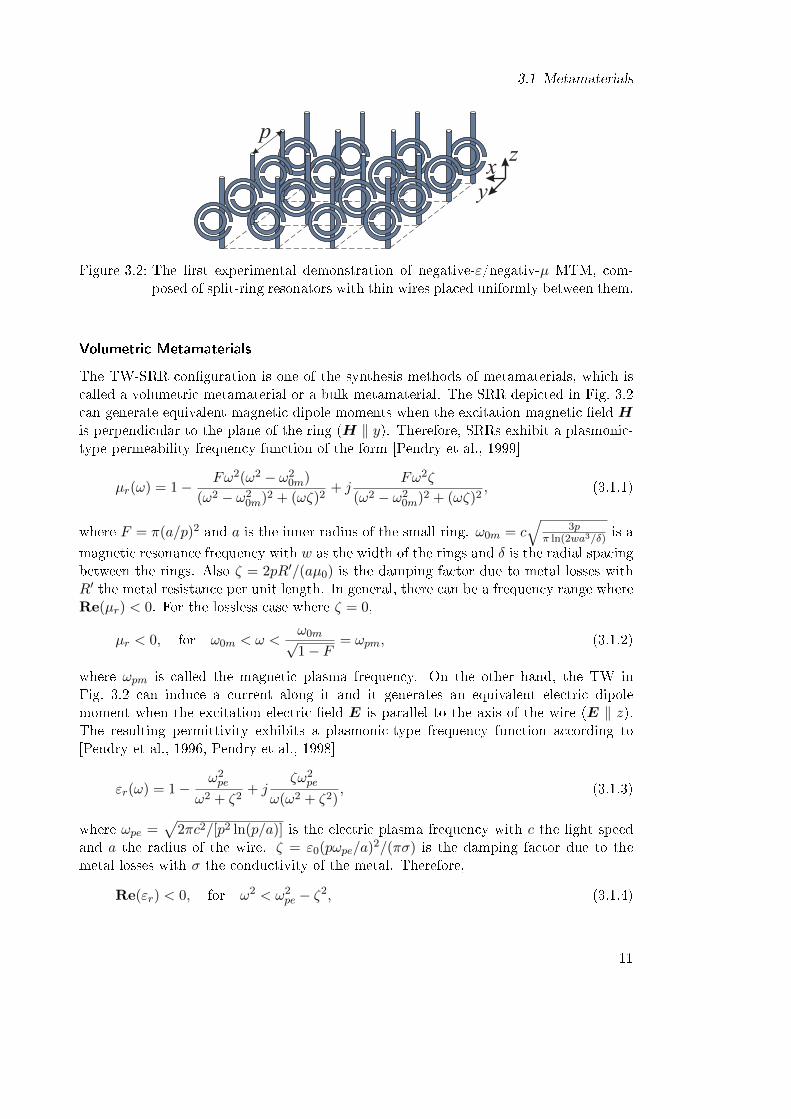
3.1 Metamaterials
p
xz
y
Figure 3.2: The rst experimental demonstration of negative-ε/negativ-µ MTM, com-posed of split-ring resonators with thin wires placed uniformly between them.
Volumetric Metamaterials
The TW-SRR conguration is one of the synthesis methods of metamaterials, which iscalled a volumetric metamaterial or a bulk metamaterial. The SRR depicted in Fig. 3.2can generate equivalent magnetic dipole moments when the excitation magnetic eld His perpendicular to the plane of the ring (H ‖ y). Therefore, SRRs exhibit a plasmonic-type permeability frequency function of the form [Pendry et al., 1999]
µr(ω) = 1− Fω2(ω2 − ω20m)
(ω2 − ω20m)2 + (ωζ)2
+ jFω2ζ
(ω2 − ω20m)2 + (ωζ)2
, (3.1.1)
where F = π(a/p)2 and a is the inner radius of the small ring. ω0m = c√
3pπ ln(2wa3/δ)
is amagnetic resonance frequency with w as the width of the rings and δ is the radial spacingbetween the rings. Also ζ = 2pR′/(aµ0) is the damping factor due to metal losses withR′ the metal resistance per unit length. In general, there can be a frequency range whereRe(µr) < 0. For the lossless case where ζ = 0,
µr < 0, for ω0m < ω <ω0m√1− F
= ωpm, (3.1.2)
where ωpm is called the magnetic plasma frequency. On the other hand, the TW inFig. 3.2 can induce a current along it and it generates an equivalent electric dipolemoment when the excitation electric eld E is parallel to the axis of the wire (E ‖ z).The resulting permittivity exhibits a plasmonic-type frequency function according to[Pendry et al., 1996, Pendry et al., 1998]
εr(ω) = 1−ω2pe
ω2 + ζ2+ j
ζω2pe
ω(ω2 + ζ2), (3.1.3)
where ωpe =√
2πc2/[p2 ln(p/a)] is the electric plasma frequency with c the light speedand a the radius of the wire. ζ = ε0(pωpe/a)2/(πσ) is the damping factor due to themetal losses with σ the conductivity of the metal. Therefore,
Re(εr) < 0, for ω2 < ω2pe − ζ2, (3.1.4)
11

3 Metamaterials and SIWs
and for ζ = 0,
εr < 0, ω < ωpe. (3.1.5)
Combining TWs and SRRs with overlapping frequency ranges of negative permittivityand permeability into a composite TW-SRR as shown in Fig. 3.2, the structure can gen-erate a substance in a frequency range with simultaneously negative permittivity andpermeability. This kind of combination normally assembles randomly or periodically thebasic elements with much smaller sizes compared to the operating wavelength to form aquasi-homogeneous metamaterial. But the volumetric MTMs have some intrinsic draw-backs. Due to the resonance characteristics of some elements, e.g. SRR, the volumetricMTMs are usually lossy and narrow-band and seem of little practical interest for theengineering applications.
Planar Metamaterials
An alternative architecture, called the planar MTM using the transmission line (TL)approach was almost simultaneously introduced by Eleftheriades et al.[IYER & Eleftheriades, 2002, Grbic & Eleftheriades, 2002], Oliner [Oliner, 2003] and Calozet al. [Caloz & Itoh, 2002, Sanada et al., 2004]. These kinds of MTMs are based on con-ventional right-handed (RH) series-L and shunt-C TLs, shown in Fig. 3.3.
Δz 0
Hm
Fm
Figure 3.3: Incremental equivalent circuit model for hypothetical uniform LH TL.
In lossy systems the wavenumber k is complex and consists of the propagation constantk′ and the attenuation constant k′′. In lossless case the propagation constant k′, the phasevelocity vp and the group velocity vg of the TL can be expressed as
12

3.1 Metamaterials
k = k′ − jk′′, (3.1.6a)
k = k′ =√Z ′Y ′ =
1
jω√L′LC
′L
= −j 1
ω√L′LC
′L
, (3.1.6b)
k′ = − 1
ω√L′LC
′L
< 0, (3.1.6c)
vp =ω
k′= −ω2
√L′LC
′L < 0, (3.1.6d)
vg = (∂k′
∂ω)−1 = ω2
√L′LC
′L > 0. (3.1.6e)
It is obvious that the phase velocity vp associated with the direction of the phase prop-agation constant k′ is negative and antiparallel to the group velocity vg which indicatesthe power ow direction in the TL. This property makes the TL in Fig. 3.3 a LH ma-terial. The planar geometry of this realization architecture brings the advantages of thecompatibility with microwave integrated circuits, the easy control of the behavior by Land C, low loss and broad bandwidth.
However, a purely LH structure does not exist, since the wave propagating in the circuitwill induce a series inductance LR and a shunt capacitor CR to the series CL and theshunt LL, respectively. Therefore, a more accurate model for the MTM design came out.A number of circuits using LH TL are based on the composite right-/left-handed (CRLH)TL model introduced by Caloz and Itoh [Caloz & Itoh, 2003]. The CRLH MTMs, whoseessential model is shown in Fig. 3.4, take the parasitic inductor LR and capacitor CRinto account.
se
sh
Figure 3.4: Equivalent circuit model for the composite right/left-handed (CRLH) MTMs.
At low frequencies, LR and CR tend to be short and open respectively, therefore theequivalent circuit will reduce to the series-CL and shunt-LL with highpass characteristics.The circuit shows the antiparallel phase and group velocities which indicates LH, asshown in Eq. (3.1.6a) to (3.1.6e), where k is the complex wavenumber, k′ the propagation
13

3 Metamaterials and SIWs
constant, vp the phase velocity and vg the group velocity. On the other hand, when thefrequency goes high, short CL and open LL leave a series-LR and shunt-CR circuit withparallel phase and group velocities, which means RH and lowpass characteristics. Whenthe series resonance frequency ωse is not equal to the shunt resonance frequency ωsh,there will be a bandgap between the LH and the RH range. However, the bandgapwill disappear if these two resonance frequencies are made equal. An innite-wavelength(λg = 2π/|k′|) propagation can be achieved at the transition frequency ωsh = ωse = ω0.Fig. 3.5 depicts the dispersion diagram for the balanced and the unbalanced CRLH TLaccording to the equivalent circuit depicted in Fig. 3.4, where LR = LL and CR = CL forthe balanced case. Many devices have been developed based on the CRLH TL showingsome advantages like bandwidth enhancement, dual-band operation, arbitrary couplinglevel as well as negative and zeroth-order resonance.
00
2
4
6
8
10
12
14
π/2 π
fse
fsh
propagation constant [m ]-1
freq
uen
cy [
GH
z]
balanced
unbalanced
Figure 3.5: Balanced and unbalanced CRLH MTMs.
1D and 2D Planar Metamaterials
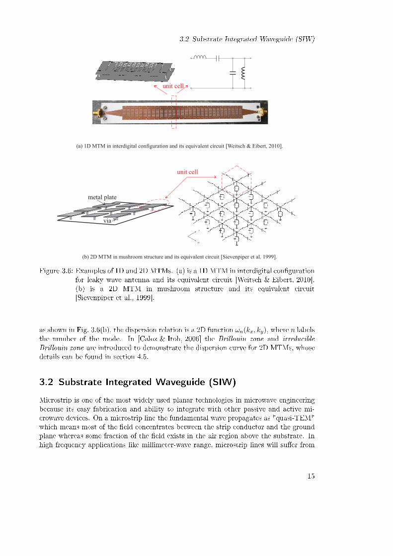
The TL theory is wildly used to realize one-dimensional (1D) MTMs, which are eec-tively homogeneous structures and can be essentially modeled by 1D transmission lines.In this kind of MTMs, the wave propagates in one dimension which can be any direc-tion in the material. The TL theory can be extended to two-dimensional structures,often named metasurfaces, where a discrete TL unit cell is dened to form a network[Caloz & Itoh, 2006, Sievenpiper et al., 1999]. Fig. 3.6 presents some examples for 1Dand 2D MTMs respectively.Due to the multi-dimensional wave propagation in 2D MTMs, e.g. in x- and y-direction
14
3.2 Substrate Integrated Waveguide (SIW)
unit cell
metal plate
via
(b) 2D MTM in mushroom structure and its equivalent circuit [Sievenpiper et al. 1999].
unit cell
(a) 1D MTM in interdigital configuration and its equivalent circuit [Weitsch & Eibert, 2010].
Figure 3.6: Examples of 1D and 2D MTMs. (a) is a 1D MTM in interdigital congurationfor leaky wave antenna and its equivalent circuit [Weitsch & Eibert, 2010].(b) is a 2D MTM in mushroom structure and its equivalent circuit[Sievenpiper et al., 1999].
as shown in Fig. 3.6(b), the dispersion relation is a 2D function ωn(kx, ky), where n labelsthe number of the mode. In [Caloz & Itoh, 2006] the Brillouin zone and irreducibleBrillouin zone are introduced to demonstrate the dispersion curve for 2D MTMs, whosedetails can be found in section 4.5.
3.2 Substrate Integrated Waveguide (SIW)
Microstrip is one of the most widely used planar technologies in microwave engineeringbecause its easy fabrication and ability to integrate with other passive and active mi-crowave devices. On a microstrip line the fundamental wave propagates as "quasi-TEM"which means most of the eld concentrates between the strip conductor and the groundplane whereas some fraction of the eld exists in the air region above the substrate. Inhigh frequency applications like millimeter-wave range, microstrip lines will suer from
15

3 Metamaterials and SIWs
high losses due to the thin conguration and the manufacturing tight tolerances. On thecontrary, high frequency hollow waveguides which have better power capacity are quitedicult to fabricate and are not compatible with planar structures. Therefore, the sub-strate integrated waveguide (SIW) which realizes a dielectric-lled waveguide in a planargeometry emerged to solve this dilemma. SIW is fabricated by using two periodic rowsof metallic vias or slots connecting the top and the bottom metal planes of a printedcircuit board (PCB) with a dielectric substrate in between as shown in Fig. 3.7. Thegeometry of SIW is suitable for mass production, low-cost fabrication and high densityintegration. SIW is one of the promising solutions for millimeter-wave applications whichis now already applied in wireless networks, automotive radars and imaging sensors witha frequency range of 60− 94 GHz [Bozzi et al., 2009].
y
zx
hw s
d
ground plate
a unit cell
Figure 3.7: The structure of a substrate integrated waveguide by using the metallic via-hole arrays.
3.2.1 Characteristics of SIWs
SIWs show similar characteristics as traditional rectangular waveguides. An SIW with awidth of w has the same propagation constant as a rectangular waveguide with a widthof wequ. Here w is the center-to-center distance between parallel sets of vias in the SIWand wequ is the width of the broad wall of the equivalent rectangular waveguide . In thecircuit design, people can calculate the equivalent width wequ as [Cassivi et al., 2002]
wequ = w − d2
0.95s, (3.2.1)
where s is the distance between the adjacent vias, and d the diameter of the via, as shownin Fig. 3.7. The cuto frequency fc for the TE10 mode of the SIW can be expressed as
fc =c
2√εr
(w − d2
0.95s). (3.2.2)
This approximation can reach ±5% accuracy in fc when s < λ0√εr/2 and s < 4d where
λ0 is the free-space wavelength and εr is the relative dielectric constant of the substrate
16

3.2 Substrate Integrated Waveguide (SIW)
of the SIW.
3.2.2 Dierent Types of SIWs
Besides the geometry depicted in Fig. 3.7, there are several dierent types of SIW. Someof them can reduce the size without changing the eld distribution. Some of them canincrease the bandwidth by reducing the cuto frequency of the fundamental mode.
• Half-mode SIW (HMSIW)The half-mode SIW depicted in Fig. 3.8 was rst proposed in 2005 by W. Hong andK. Wu [Hong et al., 2006]. The HMSIW cuts half of the SIW along the symmetricplane in the transmission direction which can be equalized to a magnetic wall (MW)and the half eld distribution keeps unchanged in the HMSIW compared to theSIW. Therefore the size of SIW can be reduced to half.
(a) The geometrical configuration of HMSIW
(b) One example of HMSIW withmicrostrip line transition [Hong et al., 2006]
(c) Domain field distribution in HMSIW[Hong et al., 2006]
Figure 3.8: The structure of a half-mode SIW and the eld distribution[Hong et al., 2006]. (a) The geometrical conguration of a HM-SIW. (b) One demonstration of HMSIW with transition to microstripline [Hong et al., 2006]. (c) Domain eld distribution in HMSIW[Hong et al., 2006].
• Folded SIW (FSIW)The folded SIW shown in Fig. 3.9 realizes the folded rectangular waveguide whichis transversely folded to form a compact structure but maintains the same propaga-tion characteristics of the conventional rectangular waveguides [Chen et al., 1988].[Grigoropoulos et al., 2005] proposed a type of FSIW by using double-layer sub-strate which can reduce the waveguide width up to (9εr)
−1/2 and overcome thediculties of manufacturing the internal vias forming the central T-septum by lami-nates and low temperature co-red ceramic (LTCC) [Grigoropoulos & Young, 2004].
17

3 Metamaterials and SIWs
2a
b εr
εr
a
2b w w
a
2b
εr
w
layer 1
layer 2
(a) rectangular waveguide (b) equivalent foldedwaveguide
(c) cross section offolded SIW in (e)
εr
TaperedStriplineExcitation
through vias
blind vias
dielectriclayers oneand two
(d) folded SIW with T-septum in[ ]Grigoropoulos & Young, 2004
w
(e) folded SIW in [Grigoropoulos et al., 2005]
Figure 3.9: The structure of FSIW. (a) The cross section of a conventional rectangularwaveguide. (b) The cross section of an equivalent folded waveguide. (c) Thecross section of an FSIW [Grigoropoulos et al., 2005]. (d) One example ofFSIW with T-septum [Grigoropoulos & Young, 2004]. (e) One example ofFSIW without T-septum [Grigoropoulos et al., 2005].
• Ridged SIW (RSIW)The ridged SIW shown in Fig. 3.10 evolves from a ridged rectangular waveguide[Hopfer, 1955]. It can reduce the cuto frequency of the fundamental mode likeTE10 mode so that the bandwidth is increased [Bao et al., 2012]. The RSIW iswildly used in WLAN antenna [Luan & Tan, 2011] and ultra-wideband[Luan & Tan, 2012] applications.
Figure 3.10: The structure of RSIW [Bao et al., 2012].
18

3.2 Substrate Integrated Waveguide (SIW)
3.2.3 Existing Modeling Methods for SIWs
Similar to rectangular waveguides, SIWs have a high quality factor and high power-handling capability compared to other planar structures like microstrip lines. But theperiodic bilateral gaps between the vias make SIWs subject to inherent leakage losses,which makes their dispersion and attenuation modeling a complicated complex eigen-problem. In former researches, the model and design of SIWs are often based on full-wave analysis tools. The numerical methods like the Finite-Dierence Time Domainmethod (FDTD), the Boundary Integral-Resonant Mode Expansion method (BI-RME),the Finite-Dierence Frequency Domain method (FDFD), or the Method of Moments(MoM)-based analysis schemes like Transverse Resonance Method have all been em-ployed to the solve the eigenproblem of SIWs. Each method has its own advantages anddisadvantages.
• The Finite Dierence Frequency Domain Method (FDFD)
The conventional FDFD usually relates the roots of the eigenproblem to the fre-quencies of a given value of the propagation constant. This makes the method nota good choice for the periodic structure which usually has complex propagationconstants. In [Xu et al., 2003] the conventional FDFD is combined with Floquet'stheorem and perfectly matched layer (PML) absorbing boundary condition (ABC)to transfer the dicult complex root-extracting problem of a transcend equationinto a generalized matrix eigenvalue problem. The Floquet's theorem for the pe-riodic structure restricts the computational layer to a single period. On the otherhand, the use of a PML ABC can eliminate the longitudinal eld components andyield an eigenproblem with its eigenvalue as the corresponding propagation con-stant. In the loss analysis, [Xu et al., 2003] equals the structure under analysis tothe resonant cavity so that the transmission distance-related attenuation constantis translated into a time-dependent damping factor.
• The Boundary Integral-Resonant Mode Expansion Method (BI-RME)
The BI-RME method provides the admittance matrix of the structure in the form ofa pole expansion in the frequency domain, relating the modal currents and voltagesat the terminal waveguide sections. It allows to derive directly the equivalent circuitlayout and nd the value of its components and avoids any initial guess or ttingprocedure. One characteristic limitation of BI-RME is that the method can only beapplied to completely shielded structures. Therefore, in structures like SIWs whichare not closed, ctitious metal walls need to be added outside the structures in orderto make them close. When the radiation leakage is negligible the ctitious metalwalls will not eect the propagation characteristics of SIWs [Bozzi et al., 2006].
• The Finite Dierence Time Domain Method (FDTD)
The FDTD method transfers the modeling of a periodic guided-wave structure tothe modeling of an equivalent resonant cavity. The equivalent resonant cavity isformed by terminating a single unit cell with the periodic boundary condition inthe propagation direction. The eigenfrequency extracted by the FDTD method
19

3 Metamaterials and SIWs
for resonators yields the desired solution in terms of frequency and quality factor.The attenuation constant can then be obtained from the extracted quality factor[Xu et al., 2007].
• The Domain Decomposition Method
The domain decomposition method combines the "domain decomposition FDTD"and the numerical thru-line (TL) calibration technique to develop an accurate andmore ecient parameter extraction of microwave circuits and structures. Using thenumerical TL calibration method, the structure under analysis can be eectivelydivided into two separate parts: error boxes and a circuit box. The error box repre-sents the potential error terms related to the port/transition discontinuities, whilethe circuit box characterizes the realistic or designed circuit properties. Instead ofusing the short-/open-circuit calibrations which are dicult to realize, the usage ofthe numerical thru-line (TL) calibration procedure can greatly remove the potentialerrors and the parasitic terms which are brought from the excitation model, thenumerical dispersion and the inherent eects of simulated structures. Especially inFDTD method, the TL calibration technology can move the position of parameterextraction into virtual normal waveguides to overcome the challenge of the separa-tion between the source and reection excitation in time domain [Xu et al., 2006].
• The Transverse Resonance Method
The transverse resonance method makes use of the concept of the surface impedanceto model the rows of the conducting cylinders and the proposed model is then solvedby combining the method of moments and the transverse resonance procedure. Inthis method the rows of cylinders in SIWs are represented as the surface impedance,which can be calculated from the reection coecient. The equivalent width ofthe SIW can be written as a function of the surface impedance. The complexpropagation constant can also be expressed as a function of the surface impedance,the equivalent width of the SIW and the frequency. Therefore, the problem ofnding the propagation constant is equivalent to a problem of nding the reectioncoecient at a desired cuto frequency. The reection coecient can be solvedwith the method of moments (MoM) technique, by discretizing the current on thecylinder surface intoN current laments along the axis of the cylinder. By using theGreen's function for a current lament in a TEM waveguide, a moment solution forthe electromagnetic scattering by a single inductive post in a rectangular waveguidecan be calculated. After calculating the current at N points on the surface ofthe cylinder, the reection coecient in the plane of the cylinder can be found[Deslandes & Wu, 2006].
3.2.4 Limitations of Existing Methods
• The methods based on the classical eigenvalue solvers, like BI-RME, or FDFD,MoM, have diculties to calculate accurately the attenuation constant due to theleakage of the SIW. Even through the calibration techniques, the methods are still
20

3.2 Substrate Integrated Waveguide (SIW)
slow for the design purpose, as they require full-wave simulations for two guidingstructures of dierent lengths.
• The MoM-based method and the Floquet-Bloch theorem require the summationof the electric elds generated by the currents on the cylinders. These elds arerepresented by a set of Hankel functions, which usually lead to a very slow con-vergence during the summation. The convergence becomes even slower when thesemi-unbounded waveguide, like SIW, presenting high leaky-wave losses, leads toan ineective calculation of the propagation constant, whose accuracy can also beseverely lowered.
21


4 Modeling of Periodic Congurations
4.1 Eigenproblem Formulation for Electromagnetic Fields
Maxwell's equations are a set of fundamental equations that govern all macroscopic elec-tromagnetic phenomena. The analysis of electromagnetic elds is actually a problemsolving a set of Maxwell's equations subject to given boundary conditions [Jin, 2002].Maxwell's equations can be considered as eigenproblems, whose eigenvalues and eigenso-lutions suciently characterize the electromagnetic systems under analysis.
4.1.1 Maxwell's Equations
Maxwell's Equations are a set of fundamental dierential equations indicating the be-havior of electromagnetic elds which were originally expressed by Maxwell in some 20equations in 1865 [Maxwell, 1873] and later rened by Heaviside to the four equationforms [Heaviside, 1888]:
∇×E = −µ∂H∂t
, (4.1.1)
∇×H = ε∂E
∂t+ J , (4.1.2)
∇ · εE = ρ, (4.1.3)
∇ · µH = 0, (4.1.4)
and
∇ · J = −∂ρ∂t, (4.1.5)
where
E = electric eld (V/m),
H = magnetic eld (A/m),
ρ = free electric charge density (C/m3),
J = free current density (A/m2),
ε = permittivity of the medium (F/m),
µ = permeability of the medium (H/m).
(4.1.6)
23

4 Modeling of Periodic Congurations
When the eld is time harmonic, the spatial and time varying elds E and H can beexpressed in the form
E(r, t) = E(r)ejωt and H(r, t) = H(r)ejωt, (4.1.7)
which transfer the Maxwell's equations (4.1.1) to (4.1.3) as
∇×E = −jωµH, (4.1.8)
∇×H = jωεE + J , (4.1.9)
∇ · εJ = −jωρ. (4.1.10)
Eq. (4.1.8) to (4.1.10) can form a set of rst-order partial dierential equations. Withappropriate initial conditions which dene the eld quantities impressed in a given volumeat an initial time, the boundary conditions which dene at any instant of time theeld quantities impressed upon the surface enclosing the given volume, and also theSommerfeld radiation condition [Jin, 2002, Bérenger, 1994, Sommerfeld, 1949]
limr→∞
r[∇×(EH
)+ jk0r ×
(EH
)] = 0, (4.1.11)
some unique solution to the set of partial dierential equation formed by Maxwell'sequations can be obtained.In Eq. (4.1.11) r = |r| and r = r/r stand for the magnitude and the direction of
the position vector r respectively. k0 is the free space wavenumber. The Sommerfeldradiation condition enforces the solution corresponding to the elds radiating from thesources to innity. Unphysical solutions, like corresponding to sinking in sources orenergy coming from innity, are omitted.
4.1.2 Helmholtz' Equations
For the time-harmonic eld, Maxwell's equations can be rewritten for both electric andmagnetic elds:
∇× (1
µ∇×E) + ω2εE = −jωJ , (4.1.12)
∇× (1
ε×H) + ω2µH = ∇× (
1
εJ). (4.1.13)
These equations are called inhomogeneous vector wave equations. For homogeneousmaterial and source-free systems, the left side of Eq. (4.1.12) and (4.1.13) can be rewrittenas the Helmholtz equations
∇2E + k2E = 0, (4.1.14)
∇2H + k2H = 0, (4.1.15)
where k = ω√εµ is the wavenumber of the medium with the dimension of 1/m.
24

4.1 Eigenproblem Formulation for Electromagnetic Fields
4.1.3 Floquet's Theorem
A periodic problem is the problem of wave propagation in a periodic structure, whichmay be characterized by periodic boundary conditions or a periodically varied dielectricconstant [Ishimaru, 1991]. According to Floquet's theorem, in an innite periodic struc-ture which is periodic in the direction of y-axis, the elds at a point y dier from theelds one period of p away by a constant attenuation and a phase shift according to
u(y +mp) = Cmu(y). (4.1.16)
Here u(y) and u(y +mp) are the wave at the point y and y +mp, respectively. m is aninteger number. The constant C is in general a complex quantity, which can be expressedas
C = e−jkp, k = k′ − jk′′, (4.1.17)
and k represents the wavenumber, where k′ is the propagation constant and k′′ is theattenuation constant. Floquet's theorem gives the possibility to represent the entireperiodic structure as one unit cell with periodic boundary considered according to
E(y)H(y)
=
Ep(y)Hp(y)
e−jkp,
Ep(y)Hp(y)
=
E(y + p)H(y + p)
. (4.1.18)
When the structure is periodic in two or even three dimension, e.g. metasurfaces, thescalar wavenumber k is replaced by a vector quantity k, called wavevector, which denesthe non-periodic functional dependence in space,
E(r)H(r)
=
Ep(r)Hp(r)
e−jk·r, (4.1.19)
where r contains the spatial periodic information with r = mpxx+ npyy+ kpz z. px, py,and pz represent the length of one unit cell in x-, y- and z-axis, respectively. k can bewritten for 3D periodic congurations as
k = kxx+ kyy + kz z. (4.1.20)
4.1.4 Eigenmodes and Eigenvalues
Eq. (4.1.12) and (4.1.13) can be considered as an operator equation according to
L(ω,k)φ = f, (4.1.21)
where f is the excitation or forcing function, and φ is the unknown quantity which canbe the electric or magnetic eld. L· represents some form of Maxwell's equations withappropriate boundary conditions and material relations and k indicates the wavevec-tor. This kind of eld problem is called boundary-value problem. In electromagnetics,eld problems are usually associated with source-free scenarios like wave propagation in
25

4 Modeling of Periodic Congurations
waveguides or the resonances in cavities, which means f vanishes and Eq. (4.1.14) and(4.1.15) are represented as
L(ω,k)φ = 0. (4.1.22)
Eq. (4.1.22) is called eigenvalue problem where both governing dierential equations andboundary conditions are homogenous. Instead of nding φ for a non-zero f , the eigenvaluepair (ω,k) is solved in an eigenvalue problem. Consequently, the corresponding φ isthe eigensolution. Eigenmodes (EMs) and eigenvalues (EVs) can uniquely determinethe characteristics of a system, like a waveguide, a resonator, or a periodic structure.In numerical solvers based on nite element (FE), nite dierence (FD), or momentsmethods, the operator equation is typically discretized and leads to a linear homogeneousequation system
[Amn(ω,k)]φn = 0. (4.1.23)
Amn are the matrix entries as a function of (ω,k) and φn are the unknown expansioncoecients of the eld solution. The eigenvalues here are pairs of (ω,k), which makethe system singular and indicate one or more propagating modes. A collection of pairsof (ω,k) covering a range of frequencies can form the dispersion behavior of the systemunder analysis. However, for large numerical systems, the solution of the eigenproblems isoften much more demanding than the solution of the corresponding driven problems andthe convergence behavior is often not satisfying. Especially periodic congurations, likemetamaterials, may often lead to eigenproblems with a considerable number of unknowns.In periodic congurations the boundary conditions can be periodic in one, two or threedimensions which can also be combined with other boundary conditions like perfectelectric conductor (PEC), perfect magnetic conductor (PMC) or absorbing boundarycondition (ABC).
4.2 Modal Series Expansion Method
One frequently used numerical method for periodic structures is a modal series expan-sion. Modal series expansion expresses the eigensolution of the inhomogeneous periodicstructure under analysis in a series expansion with the eigensolution of the homoge-neous background waveguide as the basis functions to reduce the number of unknowns.As we know, a waveguide is typically operated in the fundamental mode and only anite number of modes are relevant in the frequency range of interest. Moreover, theorthonormality and completeness of the modes make it possible to obtain the eigen-solution accurately with the expansion of just a few modes, e.g. the propagating andsome evanescent modes. For many background waveguides like rectangular waveguides,and cylindrical waveguides, the eigensolutions can be obtained analytically. For compli-cated background structures, the eigensolutions can be computed numerically by solvingeigenproblems, e.g. with CST MWS [CST, 2011]. A periodic conguration according toFloquet's theorem, can be modeled in one unit cell with periodic boundaries. Positioning
26

4.2 Modal Series Expansion Method
the periodic boundaries in the undistorted regions of the background waveguide, iden-tical to the cross section of the waveguide and perpendicular to the wave propagationdirection as depicted in Fig. 4.1, e.g. the y-direction, makes it possible to formulate theelds depending on x, z on the input periodic boundary according to
Eport,in(x, z) =
M∑m=1
[amem,port(x, z) + bmem,port(x, z)], (4.2.1)
Hport,in(x, z) =
M∑m=1
[amhm,port(x, z)− bmhm,port(x, z)], (4.2.2)
where the eigensolutions em,port and hm,port for the electric and the magnetic elds of thebackground waveguide, respectively, work as basis functions. The wave coecients amindicate the inward waves while bm refer to the outward waves. For the magnetic eld,the term with the outward wave coecient hm,port is to subtract in order to maintainan orientation in the right-hand sense. In the port planes, which are identical to thebackground waveguide cross section, the feeding modes with a number of M can beapplied to excite the structure. Every mode can excite the unit cell and couple toall other modes. Inserting the modal expansion, Eq. (4.2.1) and (4.2.2) into Floquet'stheorem expressed as Eq. (4.1.18), the eld solution at the output port can be expressedas
Eport,out(x, z) = Eport,in(x, z)e−jkp, (4.2.3)
Hport,out(x, z) = Hport,in(x, z)e−jkp, (4.2.4)
and
Eport,out(x, z) =M∑m=1
[b′mem,port(x, z) + a′mem,port(x, z)], (4.2.5)
Hport,out(x, z) =M∑m=1
[b′mhm,port(x, z)− a′mhm,port(x, z)], (4.2.6)
where L is the length of the periodic unit cell, and the complex wave number k = k′−jk′′,k′ is the propagation constant and k′′ the attenuation constant. The outgoing primedmodes b′m are related to the incident modes am and the ingoing primed modes a′m to theoutgoing modes bm according to
am = b′mejkp, (4.2.7)
bm = a′mejkp. (4.2.8)
Transfer Matrix Representation and Scattering Matrix Approach
If we consider the k-th unit cell of one periodic conguration shown in Fig. 4.2, therelationship between the amplitude of the modes at the input port and the ones at the
27

4 Modeling of Periodic Congurations
y
x
z
p
input port in place y
output port in place y+p
Figure 4.1: Unit cell of an inhomogeneous periodic structure modeled in the backgroundwaveguide with periodic boundaries.
output port can be expressed as
b1...bMa1...aM
=
T 1111 · · · T 1M
11 T 1112 · · · T 1M
12...
. . ....
.... . .
...TM1
11 · · · TMM11 TM1
12 · · · TMM12
T 1121 · · · T 1M
21 T 1122 · · · T 1M
22...
. . ....
.... . .
...TM1
21 · · · TMM21 TM1
22 · · · TMM22
a′1...a′Mb′1...b′M
. (4.2.9)
On the left side of the Eq. (4.2.9), there are the complex wave amplitudes of the modesin the input port plane, while the ones in the output port plane are grouped in thevector v = (a′1, · · · , a′M , · · · , b′1, · · · , b′M ). The transfer matrix T connects the incidentand the reected waves at the input port to the ones at the output port. IfM modes areobserved at each port, the T-matrix has a dimension of 2M×2M . The superscript of theT-parameters Tnmij indicates the coupling contribution from mode m at the output portto the mode n at the input port. The subscript indicates the coupling type. In a periodicconguration the outward wave b′ at the output port of the k-th unit cell is the inwardwave a at the input port of the (k + 1)-th unit cell which makes the T-matrix a perfectmodeling method for periodic congurations. The complete behavior T total of the totalperiodic conguration consisting of K unit cells can be expressed as a multiplication ofT k as
Ttotal =K∏k=1
Tk, (4.2.10)
where the order of the multiplication must not be changed.Take Eq. (4.2.7) and (4.2.8) into Eq. (4.2.9) then the equation can be rewritten as
ejkpv = Tkv or (Tk − ejkpI)v = 0, (4.2.11)
28

4.2 Modal Series Expansion Method
where v = (a′1, · · · , a′M , · · · , b′1, · · · , b′M ), and I is the identity matrix. Eq. (4.2.11) isin the form of an eigenproblem, where ejkp is the eigenvalue. With the determinedeigenvalue, the propagation and the attenuation constant can be obtained as
k′ = −∠(e−jkp)/p, (4.2.12)
k′′ = ln(|e−jkp|)/p, (4.2.13)
depending on frequency giving directly the dispersion and attenuation behavior of theperiodic conguration.
bk,1
ak,1
bk,M
ak,M b´k,M
a´k,M
b´k,1
a´k,1
…… Tk
Figure 4.2: The T -matrix connects the modes on the input port to the ones in the outportof the k-th unit cell.
However, the T-matrix is not directly accessible. Instead the scattering matrix whichdenes the relation of incident and reected waves at one port or from one port tothe other, can be directly obtained through some numerical full wave solvers like CST[CST, 2011] based on
Sij =biaj|ak=0 for k 6=j . (4.2.14)
In Eq. (4.2.14), Sij is found by driving port j by the incident wave aj and measuring thereected wave bi at port i where all the other ports are terminated with a matched load.Therefore, Sii is the reection coecient of port i when the incident waves at other portsare set zero and Sij is the transmission coecient from port j to port i.In some scenarios, more than one mode will be considered at each port. If in a N -port
network, as shown in Fig. 4.2, where N = 2, M modes are activated in each port, theS-matrix can be written as
b1...bMb′1...b′M
=
(S11 S12
S21 S22
)
a1...aMa′1...a′M
, (4.2.15)
where Sij =
S11ij · · · S1M
ij...
. . ....
SM1ij · · · SMM
ij
, i, j = 1, 2. (4.2.16)
29
4 Modeling of Periodic Congurations
Here the superscripts of the matrix elements indicate the modes and the subscriptsindicate the ports. Snnii is the reection coecient of mode n at port i, and Snmij indicatesthe transmission coecient of mode m at the port j to mode n at the port i, when theother inward modes are all set zero, as ak = 0, k 6= m. The S-parameters presentthe cross-coupling between the dierent modes which can be solved from the eld ina single unit cell of the periodic conguration. The procedure is known as scatteringmatrix approach (SMA) [Schuhmann et al., 2005]. With the transformation formulas[Collin, 1991]
T 11 = S12 − S11S22 \ S21, (4.2.17)
T 12 = S11 \ S21, (4.2.18)
T 21 = −S22 \ S21, (4.2.19)
T 22 = 1 \ S21, (4.2.20)
the S-matrix can be converted into the T -matrix. The \ is operated by multiplyingwith the inverse matrix. Therefore, the benets of the S-matrix and of the T -matrixcan be combined together. With the full wave simulation, the S-matrix of the unit cellcan be found, which then is converted into a T -matrix and cascaded to get the completebehavior of the periodic conguration. This procedure is quite reliable and ecient whenthe conguration can be described with a limited number of port modes. However, whenthe eld distributions are complicated or the conguration is open, the procedure mightmeet problems.
4.3 Modal Expansion for Open Structures
For a closed waveguide conguration operating normally in the fundamental mode whereonly a limited number of modes is sucient to describe the inside electromagnetic elds,the SMA technique can eciently yield accurate results. However, in an open waveguideconguration, like a leaky-wave antenna, where the series expansion of the elds is to bereplaced by an integral of a continuous spectrum of modes due to the open conguration,the SMA technique might meet a challenge. The Green's functions of the backgroundstructure can be involved in the formulation of the SMA to solve the problem of ra-diation. But the analytical spectral integral formulations of the Green's function arelimited to some canonical background congurations and the discretized integral equa-tions for periodic congurations will lead to large numbers of unknowns [Michalski, 1985,Felsen & Marcuvitz, 1994]. Several papers [Derudder et al., 1998, Derudder et al., 2001,Weitsch & Eibert, 2011] presented an alternative solution to this problem which enclosesthe open waveguide problem by a PEC shield with some articial absorbing medium,like perfectly matched layer (PML), with very low reectivity in front of it. Therefore,the integral can be avoided while the problem is closed. Moreover, the representation ina series expansion is exact.
The traditional PML which was rst introduced by Bérenger [Bérenger, 1994] is nu-merically complicated and formulated with uniaxial anisotropic material characteristics
30
4.3 Modal Expansion for Open Structures
and complex thickness. As outlined in [Derudder et al., 2001], the electromagnetic char-acteristic of PML as shown in Fig. 4.3, which has the length of dPML, can be expressedas
ε = ε0M, (4.3.1)
µ = µ0M, (4.3.2)
with
M = (α(z)x+ α(z)y + 1/α(z)z), (4.3.3)
and
α = 1 + (κ0 − 1)f(z)− j σ0
ωε0f(z). (4.3.4)
κ0, σ0, and f(z) describe the type of PML. The length of the PML dPML can be rewrittenas an isotropic layer with a complex thickness
dPML =
dPML∫0
α(z′)dz′, (4.3.5)
where z = 0 corresponds to the bottom of the PML [Teixeira & Chew, 1996]. Howeverthe numerical handling of this kind of PML is not easy.
Therefore, in [Weitsch & Eibert, 2011] a set of simple isotropic lossy absorbing lay-ers was proposed to replace the PML to avoid the numerical diculties of PML. The setof absorbing layers consists of 6 layers with the electric and magnetic losses graduallyand simultaneously increasing. The layers are designed to reduce the reection for theimpinging wave on the layers which makes the impedance of the layers
ZF0 =
õ0
ε0
√(µ′r − jµ′′r)(ε′r − jε′′r)
(4.3.6)
identical to the value of the free space impedance. In Eq. (4.3.6), µ′r = 1 and ε′r = 1 forall layers whereas µ′′r and ε
′′r stand for the electric and magnetic losses, respectively, and
stay constant over frequency. The thickness of the layers increases gradually towards totop. Tab. 4.1 gives one conguration for the absorbing layers. The absorber is placedfar away enough from the waveguide structures so that the interference on the radiationeld distribution between the waveguide and the absorber can be neglected. Meanwhilethe radiation wave can be well absorbed by the absorbing layer. Therefore, the SMAtechnique mentioned in section 4.2 can be employed with only a discrete set of modesneeded in the formulation and the scattering matrix can be eciently computed.
31

4 Modeling of Periodic Congurations
tan δ εµ
thickness [mm]
Layer 1 0.01 6
Layer 2 0.02 6
Layer 3 0.07 6
Layer 4 0.15 9
Layer 5 0.30 12
Layer 6 0.8 10
Table 4.1: Conguration of the set of absorbing layers depicted in Fig. 4.4.
z
yx
PML
PEC
substrate
air
PEC
Figure 4.3: The closed equivalence for an open waveguide structure with PML placed infront of a PEC enclosure.
sub air Layer 1 Layer 2 Layer 3 Layer 4 Layer 5 Layer 6 z
y
x
Figure 4.4: The conguration of absorbing layers.
32

4.4 Eigenproblem Solution with External Excitations
4.4 Eigenproblem Solution with External Excitations
Another method to simplify the eigenvalue searching procedure is called the method offundamental solutions (MFS), which is a boundary method for the solution of certainelliptic boundary value problems [Karageorchis, 2001]. The method approximates thesolution of the problem with a linear combination of the fundamental solutions corre-sponding to the sources (singularities) which are placed at some xed places outside thedomain of the problem. The unknown coecients of the fundamental solutions haveto satisfy the boundary conditions. This method can be applied when the fundamentalsolutions for the governing equations are available. When the propagation of electromag-netic waves is in study, the governing equations are the well-know Maxwell's equations,which can for certain congurations be simplied to the Helmholtz equation
∇2φ(P ) + k2φ(P ) = 0, P ∈ Ω, (4.4.1)
with
φ(P ) = 0, P ∈ ∂Ω, (4.4.2)
or
∂φ(P )
∂n= 0, P ∈ ∂Ω, (4.4.3)
where Ω is a bounded domain with boundary ∂Ω, P is the observation point on the bound-ary of the domain Ω, φ represents the electromagnetic wave, k is the cuto wavenumber.Eq. (4.4.2) and (4.4.3) represent the Dirichlet boundary condition and Neumann bound-ary condition, respectively. In the MFS for certain elliptic boundary value problem, thesolution φ can be approximated by a linear combination of functions in the form of
φn(c,Q;P, k) =N∑n=1
cnf1(P,Qn), P ∈ Ω, (4.4.4)
where cn are the unknown coecients, Ω is a bounded domain containing the domainΩ. Q contains the coordinates of the excitations Qn which lie outside Ω, inside Ω. Thefunction
f1(P,Qn, k) = − j4H
(2)0 (kr(P,Qn)) (4.4.5)
is a fundamental solution of the Helmholtz equation for 2D elliptic boundary valueproblems. Here r(P,Qn) represents the distance between the observation points Pand the excitations Qn, H
(2)0 is the Hankel function of the second kind of order zero
[Abramowitz & Stegun, 1984]. The excitations can be placed on the boundary ∂Ω ofthe domain Ω containing Ω while the observation points PmMm=1 are located on theboundary ∂Ω. According to the boundary conditions in Eq. (4.4.2), the coecients c aredetermined so that
33

4 Modeling of Periodic Congurations
φn(c,Q;Pm, k) = 0, m = 1, 2, . . . , N. (4.4.6)
This leads to a set of complex algebraic equations for the coecients c in the form of
G(k)c = 0, (4.4.7)
where the coecients of the matrix G can be expressed as
Gm,n(k) = − j4H
(2)0 (kr(Pm, Qn)), m, n = 1, 2, . . . , N. (4.4.8)
In order to obtain a nontrivial solution the determinant of G(k) must vanish which occursfor certain values of k. Consequently these values of k are the eigenvalues of the problem(4.4.1). This procedure is usually much easier to implement than the boundary integralequation formulation and can reach faster convergence with fewer degrees of freedomrequired but maintaining comparable accuracy. Additionally the method is robust fordierent kinds of boundary conditions. However, the former researches [Kitagawa, 1988,Kitagawa, 1991] indicated that the location of the external excitation would stronglyinuent the convergence of the method, especially for the boundaries which are notsmooth with many edges and corners.
4.5 Dispersion and Modes
The dispersion behavior is one of the focuses in periodic structure analysis. Dispersioncan be categorized in dierent classes, like mode dispersion and material dispersion. Inthis work, only the mode dispersion is studied.
Denition of Modes
The electromagnetic elds satisfy Helmholtz equations. For example, a TE or TM wavepropagates with a propagation constant β in a waveguide whose cross section is uniformalong the y-axis as shown in Fig. 4.5, the electromagnetic elds can be represented asφ(x, z)e−jβy and satisfy Helmholtz equation
(∇2t + k2
c )φ(x, z) = 0, (4.5.1)
where ∇t is the Nabla operator in the transverse plane, here the x − z plane. kc =√k2x + k2
z is called cuto wave number which is a constant quantity and depends onlyon the geometry of the guide. Once kc is obtained, the propagation constant β = ky isgiven by
β = ky =√k2 − k2
c , (4.5.2)
34
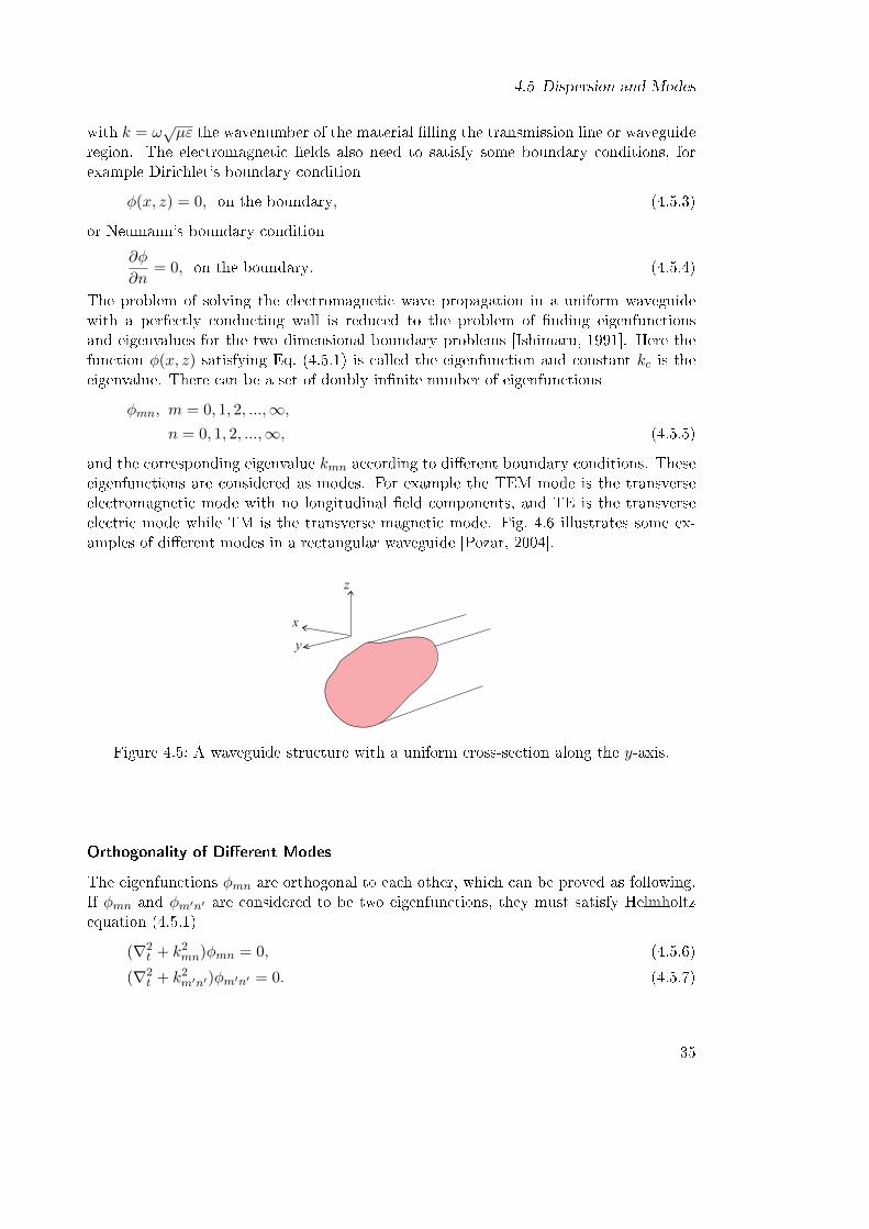
4.5 Dispersion and Modes
with k = ω√µε the wavenumber of the material lling the transmission line or waveguide
region. The electromagnetic elds also need to satisfy some boundary conditions, forexample Dirichlet's boundary condition
φ(x, z) = 0, on the boundary, (4.5.3)
or Neumann's boundary condition
∂φ
∂n= 0, on the boundary. (4.5.4)
The problem of solving the electromagnetic wave propagation in a uniform waveguidewith a perfectly conducting wall is reduced to the problem of nding eigenfunctionsand eigenvalues for the two dimensional boundary problems [Ishimaru, 1991]. Here thefunction φ(x, z) satisfying Eq. (4.5.1) is called the eigenfunction and constant kc is theeigenvalue. There can be a set of doubly innite number of eigenfunctions
φmn, m = 0, 1, 2, ...,∞,n = 0, 1, 2, ...,∞, (4.5.5)
and the corresponding eigenvalue kmn according to dierent boundary conditions. Theseeigenfunctions are considered as modes. For example the TEM mode is the transverseelectromagnetic mode with no longitudinal eld components, and TE is the transverseelectric mode while TM is the transverse magnetic mode. Fig. 4.6 illustrates some ex-amples of dierent modes in a rectangular waveguide [Pozar, 2004].
y
x
z
Figure 4.5: A waveguide structure with a uniform cross-section along the y-axis.
Orthogonality of Dierent Modes
The eigenfunctions φmn are orthogonal to each other, which can be proved as following.If φmn and φm′n′ are considered to be two eigenfunctions, they must satisfy Helmholtzequation (4.5.1)
(∇2t + k2
mn)φmn = 0, (4.5.6)
(∇2t + k2
m′n′)φm′n′ = 0. (4.5.7)
35

4 Modeling of Periodic Congurations
Figure 4.6: Field distributions for the lower-order modes of a rectangular waveguide[Pozar, 2004].
Multiply Eq. (4.5.6) with φm′n′ and Eq. (4.5.7) with φmn and subtract one from the otherto get
φm′n′∇2φmn − φmn∇2φm′n′ = (k2m′n′ − k2
mn)φmnφm′n′ . (4.5.8)
Integrating both sides of Eq. (4.5.8) with Green's second identity we can get∫l
(φm′n′
∂φmn∂n
− φmn∂φm′n′
∂n
)dl = (k2
m′n′ − k2mn)
∫sφm′n′φmnds, (4.5.9)
where s is the area of the cross section and l is the contour of it, ∂/∂n is the normalderivative with n outward from s. Since φmn and φm′n′ satisfy either Dirichlet's or Neu-mann's boundary condition as shown in Eq. (4.5.3) and (4.5.4), the left side of Eq. (4.5.9)will vanish, resulting in
(k2m′n′ − k2
mn)
∫sφm′n′φmnds = 0. (4.5.10)
Therefore, when m 6= m′ and n 6= n′, kmn 6= km′n′ , and Eq. (4.5.9) must be zero. Theeigenfunctions φmn satisfy the orthogonality condition∫
sφmnφm′n′ds = Nmnδmm′δnn′ , (4.5.11)
36

4.5 Dispersion and Modes
with
δmm′ =
1 for m = m′
0 for m 6= m′, (4.5.12)
and Nmn is the normalizing factor
Nmn =
∫sφ2mnds. (4.5.13)
The other properties of eigenfunctions can be found in appendix 10.1.
Hybrid and Degenerate Modes
Transverse modes like TEM, TE and TM are not the only cases in reality. In most cases,hybrid modes which have nonzero electric and magnetic elds in the direction of propa-gation exist. The hybrid modes are named in HEnm or EHnm depending on whether TEor TM modes are dominant [Ishimaru, 1991].
When the modes propagate at the same frequency and share the same longitudinalpropagation constant, the modes are called degenerate modes. One common exampleis in the rectangular waveguide, TEmn is degenerate with TMm′n′ when m = m′ andn = n′. Fig. 4.7 depicts the electromagnetic eld distribution of TE11 and TM11 in arectangular waveguide which has both the cuto frequency of fc = 16.145 GHz and thepropagation constant of β = 48.02 per meter. However, from the eld distribution in thecross section of the waveguide the dierent modes can be clearly distinguished.
Mode and Material Dispersions
Dispersion analysis is one of the key research topics in periodic structure studies. If awave propagates on a transmission line along the direction of y-axis, the phase velocitycan be dened as the ratio of the frequency to the propagation constant
vp = ω/ky. (4.5.14)
When ky is not a linear function of frequency, the phase velocity will be dierent fordierent frequencies ω, which means a waveform consisting of dierent frequency compo-nents will be distorted. This kind of variation of phase velocity with frequency is calleddispersion. As can be seen from Eq. (4.5.14), when ky = k as for the TEM wave, thedispersion is only due to the dielectric material lling in the waveguide or transmissionline. Therefore, it is named as material dispersion. The material dispersion is caused bythe variation of the refractive index with frequency and can be described as Sellmeier'sequation [Ishimaru, 1991] in dielectric materials.
However, for TE, TM or hybrid modes with kc 6= 0, the dispersion also dependson the mode structure. If the refraction index of the material is assumed constant over
37
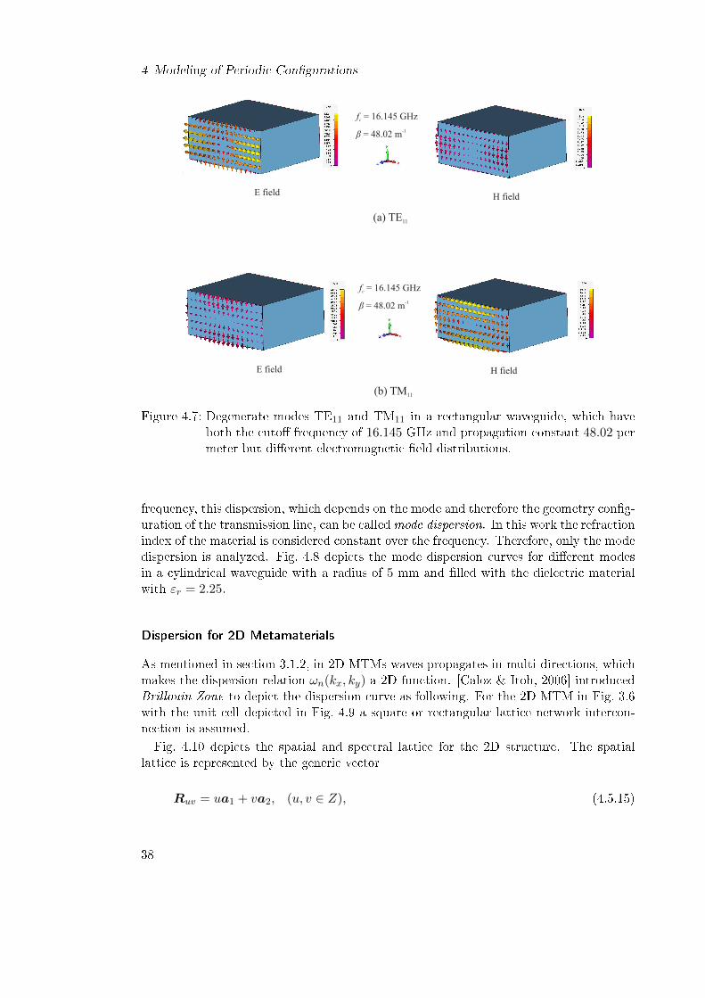
4 Modeling of Periodic Congurations
E field H field
(a) TE11
(b) TM11
H fieldE field
fc = 16.145 GHz
β = 48.02 m-1
fc = 16.145 GHz
β = 48.02 m-1
Figure 4.7: Degenerate modes TE11 and TM11 in a rectangular waveguide, which haveboth the cuto frequency of 16.145 GHz and propagation constant 48.02 permeter but dierent electromagnetic eld distributions.
frequency, this dispersion, which depends on the mode and therefore the geometry cong-uration of the transmission line, can be calledmode dispersion. In this work the refractionindex of the material is considered constant over the frequency. Therefore, only the modedispersion is analyzed. Fig. 4.8 depicts the mode dispersion curves for dierent modesin a cylindrical waveguide with a radius of 5 mm and lled with the dielectric materialwith εr = 2.25.
Dispersion for 2D Metamaterials
As mentioned in section 3.1.2, in 2D MTMs waves propagates in multi-directions, whichmakes the dispersion relation ωn(kx, ky) a 2D function. [Caloz & Itoh, 2006] introducedBrillouin Zone to depict the dispersion curve as following. For the 2D MTM in Fig. 3.6with the unit cell depicted in Fig. 4.9 a square or rectangular lattice network intercon-nection is assumed.Fig. 4.10 depicts the spatial and spectral lattice for the 2D structure. The spatial
lattice is represented by the generic vector
Ruv = ua1 + va2, (u, v ∈ Z), (4.5.15)
38

4.5 Dispersion and Modes
0 100 200 300 400 500 60011
12
13
14
15
16
17
18
19
20
propagation constant [m ]-1
freq
uen
cy [
GH
z]
TE11
TM01
fc_TE11=11.72 GHz
fc_TM01=15.31 GHz
aεr=2.25
a = 5 mm
Figure 4.8: Mode dispersion of a cylindrical waveguide with a radius of 5 mm and lledwith dielectric material with εr = 2.25. Two modes exist in 10-16 GHz, oneis TE11 with cuto frequency of 11.72 GHz and the other is TM01 with cutofrequency of 15.31 GHz.
Figure 4.9: The unit cell of the CRLH 2D network in Fig. 3.6 [Caloz & Itoh, 2006].
where
a1 = pxx and a2 = pyy. (4.5.16)
39

4 Modeling of Periodic Congurations
The spectral lattice is represented by the generic vector
Ghk = hb1 + kb2, (h, k ∈ Z), (4.5.17)
where
b1 = kxx = (2π
px)x and b2 = kyy = (
2π
py)y. (4.5.18)
One spectral period centered at the origin of Floquet function ξ(x, y) = ψ(x, y)ej(kxx+kyy)
is dened as Brillouin zone (BZ) of the periodic lattice. Brillouin zone is the squaresurface [−π/px < kx < +π/px,−π/py < ky < +π/py], which can be reduced to thetriangular surface shown in Fig. 4.10 (b) without losing the information when the latticeis symmetric with respect to the x- and y-axis. The triangular surface is called irreducibleBrillouin zone. For the computation of the dispersion diagram, the irreducible zone canbe further reduced to the segment Γ−X −M − Γ
Γ : β = 0, (4.5.19)
X : β =π
pxx (Y : β =
π
pyy), (4.5.20)
M : β = π(1
pxx+
1
pyy), (4.5.21)
while the segment includes the most important symmetry points Γ, X (also Y whenthe lattice is anisotropic) and M , where the maximum diractions take place in Braggregime [Kittel, 1964]. Therefore, the wavenumbers kx and ky along the BZ can be derivedaccording to the matrix system as [Caloz & Itoh, 2006]
Γ−X(0 < kxpx < π, kypy = 0) : kx =1
pxcos−1(1− χ
2), (4.5.22)
X −M(kxpx = π, 0 < kypy < π) : ky =1
pycos−1(3− χ
2), (4.5.23)
M − Γ(0 < kupu < π, u = x, y) : ku =1
pucos−1(1− χ
4), (4.5.24)
where χ is dened as
χ = (ω
ωR)2 + (
ωLω
)2 − κω2L, (4.5.25)
ωR =1√
LRCR(rad/s), (4.5.26)
ωL =1√LLCL
(rad/s), (4.5.27)
κ = LRCL + LLCR (s/rad)2. (4.5.28)
40

4.5 Dispersion and Modes
Figure 4.10: Square lattices for a 2D structure. (a) Spatial lattice. (b) Spectral lattice[Caloz & Itoh, 2006].
LR, CR, LL and CL are the elements that compose the equivalent circuit of the unit cellof the 2D MTM shown in Fig. 4.9. The details of the matrix system of MTMs can befound in appendix 10.2. Fig. 4.11 depicts the balanced dispersion relation of the CRLHnetwork TL of Fig. 3.6(b) in the conventional Γ−X −M −Γ diagram and the 2D curvefn(kx, ky) [Caloz & Itoh, 2006]. However, this kind of Brillouin zone depiction for thedispersion diagram is under the assumption that the attenuation of the structure can beomitted. When the attenuation is taken into account, the wavenumbers kx and ky areboth turned into complex quantities k′x− jk′′x and k′y − jk′′y , which will lead to a complex
41

4 Modeling of Periodic Congurations
phase shift ϕ = kuu, u = x, y.
12
11
10
9
8
7
6
5
4
3
2
1
0
12
11
10
9
8
7
6
5
4
3
2
1
0
12
11
10
9
8
7
6
5
4
3
2
1
0
(a)
(b)
Figure 4.11: Dispersion diagram for a 2D balanced CRLH network TL with the param-eters of Fig. 3.6(b). (a) Conventional representation along the irreducibleBZ. (b) 3D representation of the function fn(kx, ky) (n = 1, 2) over the BZ[Caloz & Itoh, 2006].
42

5 Driven Eigenproblem Computation
In the previous chapter, many full-wave modeling techniques based on classical numericalmethods for periodic congurations like SIWs and metamaterials have been introduced.However, most of them always lead to very slow convergence and often low accuracy dueto the large size, the ne details and the often open geometry of periodic congurationswhich involve complicated complex eigenproblems. Compared to the purely mathemati-cal approaches of the common eigenproblem solvers, here the driven eigenproblem solu-tion is proposed to treat the eigenproblem from a physical point of view by convertingit into an excitation problem and simplifying the eigenvalue determination by analogiz-ing the periodic structure to a resonator model [Eibert et al., 2012, Weitsch et al., 2011].According to Floquet's theorem, a periodic structure can be modeled as one appropri-ately discretized unit cell with periodic boundary conditions. Considering the unit cellas a resonator, the eigenvalue of it, the resonance frequency, can be eciently obtainedby monitoring the electromagnetic eld which usually will reach an extremum at the res-onance frequency, when an excitation is provided. This converts the eigenvalue searchingprocedure for a particular structure to a maximization of the electric eld or other observ-ables over the complex plane of the wavevector k for each frequency. The driven eigen-problem computation can be easily implemented in commercial numerical solvers likeCST MWS [CST, 2011]. However, the limited boundary exibility in CST restrains theapplication to small attenuation scenarios where the perturbation method is employedfor guided wave attenuation analysis. Consequently, the approach with CST imple-mentation is unable to analyze the attenuation inside the stop band [Chen et al., 2011].Therefore, the driven eigenproblem is implemented within the periodic hybrid nite el-ement boundary integral (FEBI) method with the innite periodic multilayer Green'sfunction [Chen et al., 2011, Eibert et al., 2011]. The implementation within FEBI candirectly consider the attenuation by a complex phase shift on the periodic boundary con-dition which makes it possible to describe the leaky and evanescent modes and computethe attenuation inside the stop band. In this chapter, the fundamentals of the driveneigenproblem computation is introduced. Then the implementation in CST for smallattenuation scenarios and the implementation in FEBI are described, respectively.
5.1 Fundamentals of Driven Eigenproblem Computation
5.1.1 Analogy between Eigenproblem and Resonator
As mentioned in chapter 4, the electromagnetic eld problem formulation can be consid-ered as an eigenproblem without excitation
L(ω,k)x = 0, (5.1.1)
43
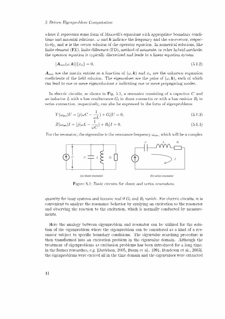
5 Driven Eigenproblem Computation
where L represents some form of Maxwell's equations with appropriate boundary condi-tions and material relations. ω and k indicate the frequency and the wavevector, respec-tively, and x is the vector solution of the operator equation. In numerical solutions, likenite element (FE), nite dierence (FD), method of moments, or other hybrid methods,the operator equation is typically discretized and leads to a linear equation system
[Amn(ω,k)]xn = 0, (5.1.2)
Amn are the matrix entries as a function of (ω,k) and xn are the unknown expansioncoecients of the eld solution. The eigenvalues are the pairs of (ω,k), each of whichcan lead to one or more eigensolutions x indicating one or more propagating modes.
In electric circuits, as shown in Fig. 5.1, a resonator consisting of a capacitor C andan inductor L with a loss conductance Gl in shunt connectin or with a loss resistor Rl inseries connection, respectively, can also be expressed in the form of eigenproblems
Y (ωres)U = [j(ωC − 1
ωL) +Gl]U = 0, (5.1.3)
Z(ωres)I = [j(ωL− 1
ωC) +Rl]I = 0. (5.1.4)
For the resonator, the eigenvalue is the resonance frequency ωres, which will be a complex
I
(a) shunt resonator (b) series resonator
Gl
Figure 5.1: Basic circuits for shunt and series resonators.
quantity for lossy systems and become real if Gl and Rl vanish. For electric circuits, it isconvenient to analyze the resonance behavior by applying an excitation to the resonatorand observing the reaction to the excitation, which is normally conducted by measure-ments.
Here the analogy between eigenproblem and resonator can be utilized for the solu-tion of the eigenproblem where the eigenproblem can be considered as a kind of a res-onator subject to specic boundary conditions. The eigenvalue searching procedure isthen transformed into an excitation problem in the eigenvalue domain. Although thetreatment of eigenproblems as excitation problems has been introduced for a long time,in the former researches, e.g. [Davidson, 2005, Baum et al., 1991, Bondeson et al., 2005],the eigenproblems were excited all in the time domain and the eigenvalues were extracted
44
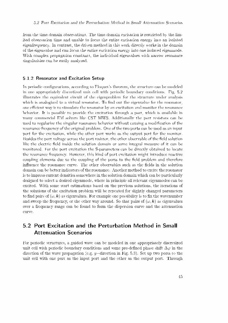
5.2 Port Excitation and the Perturbation Method in Small Attenuation Scenarios
from the time domain observations. The time domain excitation is restricted by the lim-ited observation time and unable to focus the entire excitation energy into an isolatedeigenfrequency. In contrast, the driven method in this work directly works in the domainof the eigenvalue and can focus the entire excitation energy into one isolated eigenmode.With complex propagation constants, the individual eigenvalues with narrow resonancesingularities can be easily analyzed.
5.1.2 Resonator and Excitation Setup
In periodic congurations, according to Floquet's theorem, the structure can be modeledin one appropriately discretized unit cell with periodic boundary conditions. Fig. 5.2illustrates the equivalent circuit of the eigenproblem for the structure under analysiswhich is analogized to a virtual resonator. To nd out the eigenvalue for the resonator,one ecient way is to stimulate the resonator by an excitation and monitor the resonancebehavior. It is possible to provide the excitation through a port, which is available inmany commercial EM solvers like CST MWS. Additionally the port resistors can beused to regularize the singular resonance behavior without causing a modication of theresonance frequency of the original problem. One of the two ports can be used as an inputport for the excitation, while the other port works as the output port for the monitor.Besides the port voltage across the port resistor, the other observable of the eld solutionlike the electric eld inside the solution domain or some integral measure of it can bemonitored. For the port excitation the S-parameters can be directly obtained to locatethe resonance frequency. However, this kind of port excitation might introduce reactivecoupling elements due to the coupling of the ports to the eld problem and thereforeinuence the resonance curve. The other observables such as the elds in the solutiondomain can be better indicators of the resonance. Another method to excite the resonatoris to impress current densities somewhere in the solution domain which can be particularlydesigned to select a desired eigenmode, where in principle all relevant eigenmodes can beexcited. With some start estimations based on the previous solutions, the iterations ofthe solutions of the excitation problem will be repeated for slightly changed parametersto nd pairs of (ω,k) as eigenvalues. For example one possibility is to x the wavenumberand sweep the frequency, or the other way around. So that pairs of (ω,k) as eigenvaluesover a frequency range can be found to form the dispersion curve and the attenuationcurve.
5.2 Port Excitation and the Perturbation Method in SmallAttenuation Scenarios
For periodic structures, a guided wave can be modeled in one appropriately discretizedunit cell with periodic boundary conditions and some pre-dened phase shift ∆ϕ in thedirection of the wave propagation (e.g. y−direction in Fig. 5.3). Set up two ports to theunit cell with one port as the input port and the other as the output port. Through
45
5 Driven Eigenproblem Computation
l
Port 1 Port 2
parasitic reactivecoupling element
Port 1 Port 2
ljBR
U
Excitation Observationgeneral eigenproblemas virtual resonator
(a) Equivalent circuit of eigenproblem with port excitation
(b) Equivalent circuit at resonance
Figure 5.2: Equivalent circuit of the general eigenproblem with port excitation. Depen-dent on the port conguration, a parasitic reactive coupling element can beintroduced. (b) shows the port voltage applies always on the shunt loss re-sistor of the virtual resonator, which can be used in loss calculation.
the input port the excitation can be provided to stimulate the unit cell. Meanwhile theresonance behavior can be monitored through the output port, e.g. monitoring the S-parameters over the port. With one xed phase dierence ∆ϕ the resonance frequencycan be found by sweeping the excitation frequency ω which can lead to some propagationconstant k′
k′ =∆ϕ
p=ωrescr
. (5.2.1)
Here, p is the length of the unit cell, cr is the wave propagation velocity in the material.∆ϕ is the phase dierence between the periodic boundary condition in wave propagationdirection. S-parameters can be easily used to locate the resonance frequency while thereection and transmission coecients will reach extrema at the resonance frequency.
46

5.2 Port Excitation and the Perturbation Method in Small Attenuation Scenarios
However, the reactive elements introduced by the coupling between the ports and theresonator will possibly cause a shift of the resonance frequency. As we known, the reso-nance frequency ωres is corresponding to the frequency where the transmitted power inthe unit cell is maximal. Therefore, besides the S-parameter over the port, the otherobservables like the electric eld inside the unit cell or some integral measure of it canbe monitored to reduce the inuence of the port coupling.
The losses in electromagnetic structures consist of dielectric losses, conductive lossesand radiation losses when the structures are not closed, e.g. SIWs with periodic bilateralgaps. In small attenuation scenarios, the perturbation method can be employed to ana-lyze the losses [Kong, 2009]. If a unit cell of the SIW shown in Fig. 5.3 is considered andthe y−direction is the wave propagation direction, assuming
P (y) = P (0)e−2k′′y, (5.2.2)
where P (y) is the power owing along the y−direction, P (0) is the power at the positiony = 0, and k
′′is the attenuation constant which is correspondingly obtained as
k′′
= −1
2
dP (y)
dy
1
P (y)= −1
2
∆P (y)
∆y
1
P (y). (5.2.3)
P (y) can be calculated as the integral of the time average energy at the cross sectionin propagation direction at the position y. ∆y is the length of the unit cell. ∆P (y) ishere the power lost within one unit cell, which can be dened as the power dissipated inthe loss resistor Rl of the equivalent resonator circuit as depicted in Fig. 5.2. It can becomputed with
∆P =1
2
U2
Rl, (5.2.4)
by the input voltage and the loss resistance at the resonance frequency, which are alleasily monitored at the input port.
x
y
z
s
Figure 5.3: The unit cell of a SIW as depicted in Fig. 3.7 with the port excitation in CSTMWS.
This kind of port excitation can be conveniently realized in any EM solver, e.g. thefrequency domain solver in CST MWS. However, most of them have certain drawbacks
47

5 Driven Eigenproblem Computation
like the limited boundary exibility, which allows only real phase shift on the periodicboundary leading to the inability of the description for leaky and evanescent modes.Therefore, the application will be restrained to small attenuation scenarios. Additionallydue to the intrinsic characteristics of the perturbation method, which can only analyzethe transmitted power, it is impossible to calculate the loss inside the stop band.
5.3 Current Excitation and Implementation in FEBI
The other possible excitation method such as impressed current densities somewhereinside the solution domain has some advantages over the port excitations. Without theinuence of port coupling, the current density excitation can work with an arbitraryobservable like the electric eld within the solution domain or some integral measure ofit. Additionally this excitation can be particularly designed to select a desired eigenmode,where in principle all the relevant eigenmodes can be excited [Eibert et al., 2012]. Thecurrent densities excitation can be implemented within the periodic hybrid nite-elementboundary-integral (FEBI) method with the innite periodic multilayer Green's function.The implementation in FEBI can directly consider the attenuation by a complex phaseshift on the periodic boundary condition and Green's function. Therefore, the leakyand evanescent modes can be described and the attenuation inside the stop band can becomputed.
5.3.1 Fundamentals of FEBI
Solving the governing Maxwell's partial dierential equations can help to investigate theelectromagnetic behavior of a system. However, Maxwell's equations can not be solvedanalytically except for some idealized geometries. Therefore, a number of numericalmethods has been developed to solve Maxwell's equations for complex structures. Thenite element methods and the integral equation methods, which seek the numericalsolutions for Maxwell's equations, are widely used.
Finite Element Methods
The nite element method (FEM) is a numerical technique for obtaining approximatesolutions for the boundary-value problems, which was rst proposed in the 1940s and hasbeen developed and applied extensively to dierent mathematical and engineering prob-lems [Jin, 2002]. FEM replaces the unknown function on an entire continuous domainby some simple interpolation functions with unknown coecients on a number of subdo-mains. Therefore, a nite element analysis will rst discretize or subdivide the domainof the problem, and then select the interpolation functions to form a system of equationsand nd out the solution of the system of equations. FEM permits general geometricaldiscretization elements, e.g. lines in 1D, triangles or rectangles in 2D, and tetrahedralor bricks in 3D. In electromagnetic problems, FEM solves Maxwell's equations in thedirect manner by using either the variational analysis or the weighted residuals where an
48

5.3 Current Excitation and Implementation in FEBI
electric eld formulation can be expressed as
Fv(E) =1
2
y
V
[1
µr(∇×E) · (∇×E)− k2
0εrE ·E]dv
+1
2
x
S
[E · (n×∇×E)] ds+y
V
E ·[jk0Z0Js +∇×M s
µr
]dv (5.3.1)
and
Fw(E) =y
V
[1
µr(∇×E) · (∇×W )− k2
0εrE ·W]dv
+x
S
[W · (n×∇×E)] ds+y
V
W ·[jk0Z0Js +∇×M s
µr
]dv, (5.3.2)
where V is the volume containing the sources, S represents the boundary surface of thevolume, Js and Ms are the equivalent current sources, and W is a weighting function.FEM does not include the radiation condition. Therefore, a mathematical boundarycondition or a ctitious absorbing material layer imposed outside the solution domain isrequired.
Method of Moments Solution of Integral Equation Formulation
The integral equation formulations relate the scattering or radiating eld of conductingor homogeneous dielectric materials to the unknown equivalent currents which can berepresented by Huygens' equivalent surface currents. For inhomogeneous dielectric bodiesvolumetric currents can be used, however, with expensive computational eort. TheHuygens' equivalent currents Js andM s are the tangential components of the magneticand electric elds, respectively, on a surface S enclosing the scatterer or radiator whosescattered elds Esca and Hsca external to the surface S can be considered generatedby the equivalent currents and computed using the radiation integrals [Davidson, 2005,Lu & Chew, 1995]
Esca(r) = −
S
[M s(r′) · ∇ × G(r, r′) + jk0Z0Js(r
′) · G(r, r′)]ds′, (5.3.3)
Hsca(r) =
S
[Js(r′) · ∇ × G(r, r′) + j
k0
Z0M s(r
′) · G(r, r′)]ds′, (5.3.4)
where
G(r, r′) = (I +∇∇k2
0
)e−jk0|r−r
′|
4π|r − r′|, (5.3.5)
G(r, r′) is the free space dyadic Green's function, r is a eld point and r′ represents asource point. Z0 is the free space intrinsic impedance and k0 is the free space wavenumber.
49

5 Driven Eigenproblem Computation
With the boundary conditions
n× (Einc +Esca) = 0, (5.3.6)
n× (Einc +Esca) = Js, (5.3.7)
Eq. (5.3.3) and (5.3.4) lead to the integral equation formulations. Here n is the unitvector normal to the surface and outward directed. When Eq. (5.3.6) is considered, theelectric eld integral equation (EFIE) is obtained while Eq. (5.3.7) leads to a magneticeld integral equation (MFIE). Linearly combining EFIE and MFIE to get the combinedeld integral equation (CFIE) can reduce the spurious solutions which might be causedby the singular frequencies (nonphysical interior resonances) when EFIE and MFIE areused independently on a closed surface S. The surface integral equation formulationscan make ecient analysis of the conducting and homogeneous dielectric bodies whereonly the boundary of the scatterer and radiator need to be discretized, but not forinhomogeneous penetrable materials where ctitious volumetric currents are required.
Hybrid Finite-Element Boundary-Integral Method
The hybrid nite-element boundary-integral (FEBI) method combines the advantages ofFEM and BI together. FEBI introduces an arbitrary boundary enclosing the structureunder analysis. Interior to this boundary FEM is employed, whereas surface integralequation formulations are applied to solve the eld in the region exterior to the boundary.The elds interior and exterior can be coupled by the eld continuity conditions at theboundary. This hybridization can overcome the disadvantage of domain truncation bythe mathematical boundary condition or a ctitious absorbing material layer in FEMwhich does not include the radiation condition [Davidson, 2005], as well as the expensivecomputation eort in the surface integral equation formulation for the inhomogeneouspenetrable materials where the ctitious equivalent volumetric currents are required.
5.3.2 Implementation of the Driven Method in FEBI
Consider a 2D innite periodic conguration as illustrated in Fig. 5.4. The geometry orthe material distribution is periodic along the x- and y-axis with lattice vector ρa andρb, respectively. In direction of the z-axis the conguration is divided into several layers.The possibly inhomogeneous parts are included in one layer, which can be representedin a unit cell and discretized with a tetrahedral mesh. Above and below the possiblyinhomogeneous layer, there might be some homogeneous layers, which can also be rep-resented with the lattice vectors ρa and ρb. According to Floquet's theorem, the eldsin the structure can be expressed as
E(r +mρa + nρb) = E(r)e−jkt00·(mρa+nρb), (5.3.8)
H(r +mρa + nρb) = H(r)e−jkt00·(mρa+nρb), (5.3.9)
with
kt00 = kx00x+ ky00y. (5.3.10)
50

5.3 Current Excitation and Implementation in FEBI
Here, kt00 is the wavevector parallel to the xy-plane and corresponding to the (00)th
Floquet mode. The elds are solved by FEBI [Eibert et al., 1999] which solves the tetra-hedral mesh cell using FE with some periodic boundary conditions (PBCs) where thecomplex kt00 can be considered directly for the lossy structures. On the other hand, onthe planar top and bottom surfaces of the FE unit cell mesh and the homogeneous layersabove and below it, BI is employed to solve the radiation and scattering of the structurewith the appropriate spectral domain 2D periodic Green's functions [Eibert et al., 2003].Details about the periodic Green's function can be found in appendix 10.3. For the freespace above and below the unit cell, the spectral representation of the scalar half-spaceGreen's function of Helmholtz equation
G(r, r′) =
+∞∑m=−∞
+∞∑n=−∞
e−jktmn·(ρ−ρ′)
2Ajkzmne−jkzmn|z−z
′|, (5.3.11)
can be used. ρ is the projection of the eld point r on the xy-plane with r = ρ + zz.A = |ρa× ρb| is the cross-section area of the unit cell's top or bottom boundary surface.
kzmn = ±√k2
0 − ktmn · ktmn, (5.3.12)
ktmn = kt00 +2π
A[n(z × ρa) +m(ρb × z)], (5.3.13)
are the wavevector of the (mn)th Floquet mode along the z-axis and in xy-plane, re-spectively. With the complex kt00 and the free space wavenumber k0 = ω
√µ0ε0, the BI
representation will induce a nonlinear eigenproblem.
As mentioned in section 5.1, the nonlinear eigenproblem of periodic congurationscan be solved by solving the corresponding excitation problem in the domain of theeigenvalue. This can be done by analogizing the unit cell of the periodic structure into aresonator and nd the resonance frequency as the eigenvalue by stimulating the resonatorwith an excitation. In FEBI, other than the port excitations, the current densities ex-citation which has more mode excitation and observable selection exibility is selected.Compared to the port excitation, impressed current densities excitation can stimulate onemode more eciently than the other, so called mode selection. On the other hand, withappropriately arranged electric and magnetic current sources with dierent polarizationsor distributions inside the solution domain, all the relevant modes can be excited, sinceelectric and magnetic elds of one mode are never exactly zero at identical locations[Eibert et al., 2012]. Additionally, for the loss analysis, instead of monitoring the voltageacross the port resistors, other observables like the electrical eld or the integral measureof it can be monitored to nd the resonance frequency. With some start estimationsbased on the previous solutions, the iterations of the solutions of the excitation problemwill be repeated for slightly changed parameters. One possibility is to x the wavevectork and sweep the frequency ω till the resonance frequency is found. The other way is tomake the frequency constant and vary the wavevector which can be considered as a com-plex quantity so that the propagation modes with stronger attenuations, e.g. evanescentmodes or leaky modes, can be monitored.
51

5 Driven Eigenproblem Computation
z
y
x
ρb
ρa
homogeneouslayers
possiblyinhomogeneouslayer
Figure 5.4: 2D innite periodic conguration.
5.4 Complex Waves
One important topic in the driven method is how to choose the correct sign for thewavenumbers in Eq. (5.3.12). In the open waveguiding conguration, the boundariesare extended to innity in some direction making discrete modes, which exist in closedwaveguiding structures, fall together and merge into a continuous spectrum of modes.Additionally a discrete set of modes can exist for the surface waves. Here the class of geo-metrical conguration depicted in Fig. 5.5 is considered, which consists of a semi-innitefree-space region bounded by a plane interface which can be either a reactive surface,an ideal conductor, a lossy sheet, or a transition air-media interface. The boundarycondition, which is assumed to be independent in x- and y-direction, can be expressedas an impedance function Zi(kz) for every single mode i in the transverse z-direction.kz denotes the transverse wavenumber and a characteristic of the corresponding modes.One line source of either electric or magnetic type is placed at y = 0 and parallel to thex-axis. Therefore, the longitudinal representation of modes traveling in z−direction atand above the interface z ≥ 0 can be expressed as
G(y, z) =1
2
∞∫−∞
f(ky)e−jkyye−jkzzdky, (5.4.1)
which is with a time dependence ejωt and consists of a continuous spectrum with thepurely real eigenvalues ranging from negative to positive innity. f(kz) is a amplitudefunction depending on the impedance function Zi(kz) of the interface as well as the loca-tion of the line source. The electric or magnetic line current source will excite TM or TEmodes, respectively. G(y, z) is proportional to the x-component of each mode and repre-sents the eld expansion as a Fourier transform with respect to ky when the integrationis performed along the real axis in the complex ky-plane according to [Sommerfeld, 1949].ky and kz are the wavenumbers along y- and z-axis, which satisfy the relation
ky = ±√k2
0 − k2z (5.4.2)
52

5.4 Complex Waves
where k0 = ω√µ0ε0 is the wavenumber of free space. A two-sheet Riemann surface can be
used to interpret the square root function shown in Eq. (5.4.2) where one sheet presentsone value or branch and the second sheet is for the other value. The two sheets are linkedby arbitrary branch cuts connecting branch points, in Eq. (5.4.2) one pair of which iskz = ±k0 and another one is assumed at∞. Therefore, the Riemann surface is separatedby the branch cuts extended from the branch points ±k0 to innity and categorized asproper and improper sheets according to physically reasonable and unreasonable eldsolution, respectively. Additionally the original Sommerfeld integration path along thereal ky-axis is deformed by the branch cuts in the complex ky-plane. According tothe Sommerfeld radiation condition, the proper solution of the problem must vanish atinnity which makes the considered conguration in Fig. 5.5 as
Im(kz) < 0, where kz = k′z − jk′′z (5.4.3)
to make sure the wave decays with z → ∞. Consequently only the lower half of thekz-plane satises the requirement. Choose the branch cut so that the proper plane whichis here the lower half of the kz-plane is plotted on the top sheet of the two-sheetedRiemann ky-plane [Tamir & Oliner, 1963] depicted in Fig. 5.6. The upper half of thekz-plane which is plotted on the bottom sheet of the Riemann plane is improper. Thebranch cuts for Im(kz) = 0 and the assumption of innitesimal losses for the free spacewavenumber
0 < |Im(k0)2| < |k20|, (5.4.4)
can ensure the integration of Eq. (5.4.1) to be along the entire real ky-axis which isalso known as Sommerfeld integration path. Comparing to other branch cuts, this kindof branch cut can make the transverse integral representation obtained by a contourdeformation a spectral one [Collin, 1991].
y
z
x
θ
r
Z ki z( )free space
Figure 5.5: Conguration of the plane interface.
If Eq. (5.4.1) is considered in the complex kz-plane, the transverse representation ofthe eld can be obtained. The former Sommerfeld integration path P is deformed andtransformed to a semicircle at innity for the positive y, as path P ′ shown in Fig. 5.6.For the negative y, the semicircle will be in the upper half of the top Riemann sheet.Innity does not contribute to the integral. Therefore, according to Cauchy's theorem
53

5 Driven Eigenproblem Computation
j kIm( )y
Re( )ky
Re( )>0kz
Re( )>0kz
Re( )<0kz
Re( )<0kz
-k0
k0
branch point
branch point
branch cut
branch cut
Sommerfeld path P
P’
Figure 5.6: The proper Riemann sheet of ky-plane, where Im(kz) < 0.
for complex integration Eq. (5.4.1) can be rewritten as
G(y, z) =1
2π
∞∫−∞
(f(ky)e−jkyye−jkzz
dkydkz
)dkz + 2πj∑
residues
, (5.4.5)
where the integration is performed along the entire real kz-axis which is the path aroundthe branch cuts. The residues caused by the possible pole singularity can be proper andcorrespondent to the complex waves which are also called surface waves when the residueslocate in the top Riemann sheet of the ky-plane whereas the improper waves locate in thelower Riemann sheet of the ky-plane will never be captured by the path P ′. Comparedto the longitudinal representation in Eq. (5.4.1) which can only generate a continuousspectrum corresponding to the radiation waves which are not bounded to the interface,the transverse representation in Eq. (5.4.5) can yield additionally a discrete spectrumrepresenting the discrete waves associated with a waveguide. Tab. 5.1 summaries somerelations between proper/improper waves and the wavenumbers ky and kz when k′y > 0[Ishimaru, 1991].
Complex Floquet Modes with Attenuations
As shown in Fig. 5.7, real Floquet modes are interpreted as discrete samples along theSommerfeld integration path for non-periodic congurations. If complex Floquet modeswith attenuations in the power ow direction are considered, Im(ky) becomes negativeand deforms the discrete samples as depicted in Fig. 5.7. All complex modes remain onthe top Riemann sheet, which are proper, except the modes which are located between theorigin and the branch point k. These modes cross the branch cut through a deformationof the Sommerfeld integration path and move to the lower improper Riemann sheet.
54

5.4 Complex Waves
Case k′y k′′y k′z k′′z Wave
+ 0 + 0 fast wave (waveguide modes)
proper wave
+ − + + backward leaky wave
+ 0 0 + trapped surface wave
+ + − + Zenneck wave
+ 0 − 0 plane-wave incidence
improper wave
+ − − −
+ 0 0 − untrapped surface wave
+ + + − forward leaky wave
Table 5.1: Proper and improper waves in geometry conguration shown in Fig. 5.5 asso-ciated with wavenumber ky = k′y − jk′′y and kz = k′z − jk′′z .
j kIm( )y
Re( )ky
Re( )>0kz
Re( )>0kz
Re( )<0kz
Re( )<0kz
-k0
k0
branch point
branch point
branch cut
branch cut
Sommerfeld path Preal Floquet modes
complex Floquet modes improper mode
Figure 5.7: The real and complex Floquet modes in the complex transverse wavenumberplane of ky, where Im(kz) < 0 and kx = 0, for the waveguide structure asdepicted in Fig. 5.5.
Fast and Slow Waves In Leaky-wave Antenna
If the interface in Fig. 5.5 is considered as surface of a leaky-wave antenna, Eq. (5.4.2)can be rewritten as
kz = ±√k2 − k2
y, (5.4.6)
55

5 Driven Eigenproblem Computation
when the laterally constant eld distribution in x-direction, kx = 0 is assumed. A scalarplane wave can be represented as
ψ(y, z) = ψ0e−jkyye−jkzz. (5.4.7)
Therefore, the propagation of the eld can be divided into two caseskz ∈ Re if |ky| < k0,
kz ∈ jIm if |ky| > k0.(5.4.8)
An imaginary kz will make the corresponding exponent in Eq. (5.4.7) real which meansno wave radiation in positive z-direction. Fig. 5.8 demonstrates the relation. The lightline where |ky| = k0 separates the radiation and purely guided waves.
light linelight line
fast wave region radiation possible
slow wave regionradiation impossible
slow wave regionradiation impossible
Figure 5.8: The fast and slow wave regions separated by the light line, indicating radiatingwaves and purely guided waves.
56
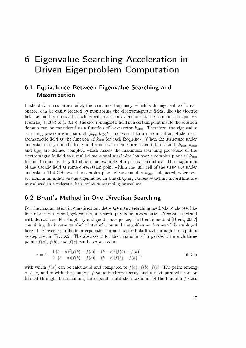
6 Eigenvalue Searching Acceleration in
Driven Eigenproblem Computation
6.1 Equivalence Between Eigenvalue Searching andMaximization
In the driven resonator model, the resonance frequency, which is the eigenvalue of a res-onator, can be easily located by monitoring the electromagnetic elds, like the electriceld or another observable, which will reach an extremum at the resonance frequency.From Eq. (5.3.8) to (5.3.10), the electromagnetic eld in a certain point inside the solutiondomain can be considered as a function of wavevector kk00. Therefore, the eigenvaluesearching procedure of pairs of (ωres,kt00) is converted to a maximization of the elec-tromagnetic eld as the function of kt00 for each frequency. When the structure underanalysis is lossy and the leaky and evanescent modes are taken into account, kt00, kx00
and ky00 are dened complex, which makes the maximum searching procedure of theelectromagnetic eld as a multi-dimensional maximization over a complex plane of kt00
for one frequency. Fig. 6.1 shows one example of a periodic structure. The magnitudeof the electric eld at some observation point within the unit cell of the structure underanalysis at 11.4 GHz over the complex plane of wavenumber ky00 is depicted, where ev-ery maximum indicates one eigenmode. In this chapter, various searching algorithms areintroduced to accelerate the maximum searching procedure.
6.2 Brent's Method in One Direction Searching
For the maximization in one direction, there are many searching methods to choose, likelinear bracket method, golden section search, parabolic interpolation, Newton's methodwith derivatives. For simplicity and good convergence, the Brent's method [Brent, 2002]combining the inverse parabolic interpolation and the golden section search is employedhere. The inverse parabolic interpolation forms the parabola tted through three pointsas depicted in Fig. 6.2. The abscissa x for the maximum of a parabola through threepoints f(a), f(b), and f(c) can be expressed as
x = b− 1
2
(b− a)2[f(b)− f(c)]− (b− c)2[f(b)− f(a)]
(b− a)[f(b)− f(c)]− (b− c)[f(b)− f(a)], (6.2.1)
with which f(x) can be calculated and compared to f(a), f(b), f(c). The point amonga, b, c, and x with the smallest f value is thrown away and a next parabola can beformed through the remaining three points until the maximum of the function f does
57
6 Eigenvalue Searching Acceleration in Driven Eigenproblem Computation
Figure 6.1: Magnitude of electric eld at some observation point within the unit cellof a periodic structure at 11.4 GHz over the complex plane of wavenumberky00 = k′y − jk′′y when attenuation is considered.
not change any more. The golden section search is to divide the searching range intotwo sections with the ratio of r/(1− r), where r = 0.61803 and to locate the maximumin one of the two sections to narrow down the searching range, as shown in Fig. 6.3.The Brent's method switches between the inverse parabolic interpolation and the goldensection search to make sure every step converges and prevent the iterations to bouncearound in some nonconvergent limit cycle [Brent, 2002].
6.3 Powell's Quadratically Convergent Method inMulti-direction Searching
As already mentioned before, the eigenvalue determination of the resonator model canbe considered as a multi-dimensional maximization of the chosen observable over thecomplex plane of kt00, where kt00 = kx00x+ky00y, kx00 = k′x−jk′′x and ky00 = k′y−jk′′y . Torealize the multi-dimensional search eciently, a set of N mutually conjugate directionsui is set up rstly and then from one initial point P0 we search along ui for the maximumPi and use it as the initial point for the next search along direction ui+1. Repeat thisstep until the function stops increasing. Every time after all the N directions have beensearched, (2PN − P0) is evaluated as an extrapolated point and its observable valueis compared to the observable values of P0 and PN and it is decided, whether a newaverage direction needs to be chosen. This can help the algorithm to take advantage
58

6.3 Powell's Quadratically Convergent Method in Multi-direction Searching
0 2 4 6 8 10 12-60
-40
-20
0
20
40
60
80
x
f(x)
function need to be optimized
parabola through 1, 2, 3
parabola through 2, 4, 3
1
2
3
4
Figure 6.2: Inverse parabolic interpolation.
r( )1-r
4
5
6
(1-r) r
(1-r) r
rf(x)
3
1
2
Figure 6.3: Golden section search.
of the direction with the largest increase as well as to keep the directions conjugate[Brent, 2002]. This acceleration method works well for local maximization where onlyone maximum happens according to the only one mode in a certain frequency range.However, sometimes there are more than one mode existing simultaneously in the samefrequency range. Therefore, all the maxima must be located.
59

6 Eigenvalue Searching Acceleration in Driven Eigenproblem Computation
6.4 Global Optimization for Multi-mode Scenario
When there are more than one mode propagating in the operating frequency range, con-sequently there will be more than one maximum in the complex plane of wavenumber asshown in Fig. 6.1. In order to obtain the mode dispersion behavior of all the propagatingmodes, it requires to locate all the maxima which actually leads to a global optimizationover the complex plane of the wavenumber.
Global Optimization: Problem and Classication of Algorithms
Many problems in engineering and science can be formulated as global optimization prob-lems. The goal of the global optimization is to nd the best possible elements x∗ froma set X according to a set of criteria F = f1, f2, . . . , fn [Weise, 2008]. These criteria areexpressed as mathematical functions, the so-called objective functions. The objectivefunctions in many practical applications are not convex which leads to multiple local andglobal extremal points in the region of interest. The determination of these local extremacan be one step in a procedure to nd the global extrema. However, nding all these mul-tiple extrema is a challenging computational problem. Unlike the local extrema, thereis no practical and general criteria to determine whether a global extremum is foundwhich makes the problem even worse. Therefore, the existing methods like deterministicand stochastic methods are basically searching the region of interest systematically dueto the lack of the local criteria for the ascertaining global extrema. However, it is notcomputationally feasible to search exhaustively over a ne mesh unless the dimension ofthe parameter space is small. How to search it eciently is the main challenge of thesealgorithms.
According to the method of operation, generally the optimization algorithms can be di-vided into two categories: deterministic and probabilistic algorithms. The deterministicalgorithms are usually used in the problem where a clear relation between the character-istics of the possible solutions and their utility exists. The search space can be ecientlyexplored for example by divide and conquer scheme (D&C). When the relation betweena solution candidate and its utilities in the given problem is not so obvious or too compli-cated, or the dimensionality of the search space is very high, the probabilistic algorithmsare better choices. This class of algorithms trades the guaranteed correctness of the solu-tion to a shorter runtime where the solution can not be guaranteed as a global optimum.Both algorithms use heuristics which are the functions helping to decide which one ofa set of possible solutions to be examined next. The deterministic algorithms normallyemploy heuristics to dene the processing order of the solution candidates. While theprobabilistic algorithms tend to consider the selected elements by the heuristic of thesearch space in further computations. Most global optimization algorithms can be di-vided into two separate phases. One is the global phase where the exhaustive explorationof the search space is conducted. The other is the local phase, which exists in each itera-tion of the global phase and employs a local optimization procedure to identify a locallyoptimal point.
60

6.4 Global Optimization for Multi-mode Scenario
• Deterministic AlgorithmsAn algorithm is deterministic if it can be simulated by a deterministic nite au-tomaton, that is, a 5-tuple (
∑, Q, q0, F, δ) where
∑is the input alphabet, Q the set
of states, q0 ∈ Q the start state, F ⊆ Q the set of nial states, and δ : Q×∑→ Q
is the transition function [Liberti, 2008]. The transition function produce the nextstate with the current state of the automaton and a word from the input alpha-bet. The well-dened function δ embodies the principle of determinism which canproduce a unique next state to any pair of (current state, input word). When thenext state is a subset of Q, which leads to more than one possible next states toany pair (current state, input word), the automaton is a nondeterministic niteautomaton. However, any nondeterministic nite automaton can be simulated bya deterministic nite automaton. Computers are theoretically deterministic niteautomata while they are instructed to perform certain steps. Therefore, the algo-rithms can run on the deterministic computers based on transition relations ratherthan functions. Both, the global phase and the local phase can be deterministic.The most famous and wildly used deterministic algorithms are
Branch-and-Select methods [Tuy, 1998]Branch-and-Select methods include branch-and-bound and branch-and-cuttechniques. The branch-and-bound can be divided into two stages, one issplitting the problem space into subspaces and the other is calculating lowerand/or upper bounds for the objective function value of the subspaces. Thefunction value of the bounds are compared and the subspaces can be decidedwhether to be discarded or not. The brand-and-cut technique is a combina-tion of the brand-and-bound techniques and the cutting plane method butits applications are restricted to integer linear problems. When the obtainedpossible solution contains a non-integer value for a variable which is supposedto be integer, the cutting plane method is employed to nd further linearconstraints that are satised by all feasible integer points.
Outer approximation method [Duran & Grossmann, 1986]The outer approximation method alternately solves a primal problem whichis a nonlinear program with all the integer variables xed in value and arelaxed master problem which is a mixed-integer linear program constructedby linearizing the objective function and the constraints around a solutionpoint of the primal problem. At each iteration, the updated best primalsolution provides a lower bound in the maximization case and the relaxedmaster problem gives an upper bound for the optimal solution. Then the nextinteger value can be determined. When the upper bound converges to thelower bound, the global optimum is obtained.
Methods based on algebraic geometry [Basu et al., 2006]Algebraic geometry is a combination of linear algebra, where the systems oflinear equations with several variables are studied, and algebra where the
61

6 Eigenvalue Searching Acceleration in Driven Eigenproblem Computation
polynomial equations with one variable are studied. The algebraic geometryhelps to describe the geometric structure of the set of solutions for polynomialequation systems with several variables when the solutions can not be explic-itly written down. This concept can be applied to nd the global optimum ofa system when the objective function can be expressed polynomially. Manyapplications can be found [Kavasseri, 2007], [Jibetean & de Klerk, 2006].
• Stochastic algorithmsThe stochastic algorithms deal with situations with a random element in the choiceof the next step of computation. The deterministic automata e.g. computers needto simulate the random choices with pseudo-random number sequences or similarcomputational devices or employ a random external input for the true randomdata requirement. The stochastic algorithms work usually in global phase. SeveralMonte-Carlo-based algorithms exist:
Simulated annealing (SA) [Kirkpatrick et al., 1983], [erný, 1985]The simulated annealing method is often used to locate a good approxima-tion to the global optimum of a given function in a large search space. Themethod is inspired by the physical process of annealing in metallurgy whichuses heating and cooling of a material to increase the size of its crystals toreduce their defects. Similar to the atoms' movement of escaping from theinitial state and wandering randomly through states of higher energy whenheating, SA replaces the current solution by a random solution. The newsolution can be found by reducing a global parameter T and comparing thedierence between the corresponding function values, similar as atoms tendto lower internal energy states when it is cooling.
Random optimization (RO) [Matyas, 1965], [Baba, 1981]Random optimization iteratively moves the solution to a better position in thesearch space which is sampled using for example a normal distribution aroundthe current position. It does not employ the gradient of the problem to beoptimized. Therefore, it can work with functions which are not continuous ordierentiable.
Evolutionary Computation (EC)Evolutionary computation is a subeld of articial intelligence that involvescombinatorial optimization problems. It includes dierent algorithms e.g. evo-lutionary algorithms (EA) which are generic population-based metaheuristicoptimization algorithms, a learning classier system (LCS) which is with closelink to reinforcement learning and genetic algorithms, evolutionary program-ming, evolution strategy (ES), or genetic programming (GP). EC uses iterativeprogress e.g. growth or development in a population which is then selected ina guided random search using parallel processing to achieve the desired end.
Methods based on Monte Carlo Sampling [Metropolis & Ulam, 1949]The Monte Carlo methods basically rely on repeated random sampling tocompute their results. They are wildly used in simulating systems with many
62

6.4 Global Optimization for Multi-mode Scenario
coupled degrees of freedom, e.g. uids, disordered materials, strongly coupledsolids, and cellular structures or modeling the phenomena with signicantuncertainty in inputs, e.g. the calculation of risk in business. The methodsbased on Monte Carlo sampling always follow some certain steps. First adomain of possible inputs must be dened. Then the inputs are generatedrandomly from a probability distribution over the domain and a deterministiccomputation is performed on the inputs. Finally the results are aggregated[Kalos & Whitlock, 2008].
Parallel tempering [Swendsen & Wang, 1986], [Earl & Deem, 2005]The parallel tempering tries to improve the dynamic properties of the MonteCarlo method, also named as replica exchange Markov chain Monte Carlo(MCMC) sampling. A Monte Carlo simulation performs a single stochasticprocess to evaluate the energy of the system and decides whether to accept orreject the updates based on the temperature T . However, when the system ishighly correlated the system can suer from critical slowing down of conver-gence due to the high rejection of updates. The parallel tempering is to makethe congurations at high temperatures, where the updates are comparativelymore probable, also available to the simulations at low temperatures and viceversa. Therefore, the method can sample both low and high energy cong-urations and become very robust. The thermodynamical properties whichare generally dicult to compute in the canonical ensemble can be computedprecisely.
Stochastic tunneling (STUN) [Hamacher, 2006], [Hamacher & Wenzel, 1999]The stochastic tunneling is also based on the Monte Carlo method. It isdesigned to avoid the slow dynamics of ill-shaped energy functions which mightbe encountered by Monte Carlo method when hopping randomly from thecurrent solution vector to another one. Instead of sampling the objectivefunction, the stochastic tunneling samples a transformed function that lacksthe slow dynamics, whose standard form can be dened by the expectation ofthe dierence between the optimal function value found so far and the nextfunction value.
Combined Trajectory Methods for Global Optimization
In this work, the relation between the solution (ω,k) and the objective function e.g. theelectromagnetic eld is complicated but clear. Therefore the deterministic algorithmscan be employed to nd the multiple extrema over the complex plane of wavevector. Themethods of nding the local extrema stated in chapter 6.2 and 6.3 can eciently locateone stationary point in the region. However the diculty lays on how can the searchingscheme escape from one found stationary point and nd the possible direction for thenext one. [Yang & Beck, 1998] introduced a combination of two generalized trajectorymethods for computation of multiple local extrema of an objective function. One tra-jectory method is a homotopy one which can nd a stationary point of the objective
63

6 Eigenvalue Searching Acceleration in Driven Eigenproblem Computation
function with global convergence. Then the second method, named a relaxation scheme,can systematically connect other stationary points in a region from a starting stationarypoint by a network of trajectories.
• Homotopy schemesThe homotopy schemes are also named embedding, invariant embedding, and pa-rameter continuation. The main idea of the homotopy schemes is to transform thetarget problem which is dicult to solve into a simpler problem by embedding thetarget problem and the simple one into a more general problem with a transitionfunction called a homotopy. The transformation can be described by a homotopyparameter which can be changed continuously in order to evolve the simple solu-tion into the target solution [Garcia & Gould, 1980], [Keller, 1987]. Dierent fromlocal iterative methods, the homotopy schemes have the characteristics of globalconvergence, which means they do not require good initial guesses in order to con-verge. This feature makes the homotopy schemes good choices for highly nonlinearproblems where good initial guesses are dicult to estimate. If f(x) is consideredas the objective function which needs to be solved, the stationary points of f(x)satisfy the stationary condition
∇f(x) = 0. (6.4.1)
Therefore, the problem of nding all the stationary points of f(x) is actually theproblem of nding all the roots of the set of equations in (6.4.1). The homotopyschemes try to embed (6.4.1) in a new set of equations
g(x, λ) = 0, λ ∈ R. (6.4.2)
Here g(x, λ) ∈ Rn and all the roots of (6.4.1) also satisfy (6.4.2) for some particularvalue of λ. There are two main canonical homotopy schemes, Newton and xed-point. In xed-point homotopy, Eq. (6.4.2) is dened as
gF (x, λ) = (1− λ)Mf (x− x0) + λ∇f(x) = 0, (6.4.3)
where x0 is a xed arbitrary point in the search region andMF is a nonsingular n×nmatrix. The homotopy trajectory is traced by varying λ from 0 to 1. When λ = 0,Eq. (6.4.3) is turned into the simple problem with only one solution x = x0. Whenλ = 1, Eq. (6.4.3) is the original problem. In Newton homotopy, the derivative ofthe objective is required and Eq. 6.4.2 is rewritten as,
gN (x, λ) = (1− λ)(∇f(x)−∇f(x0)) + λ∇f(x) = 0. (6.4.4)
• Relaxation schemesAfter nding one stationary point by using the homotopy scheme, the relaxationschemes can be employed to determine the other stationary points in the searchingspace. The idea is to use a special form of Eq. (6.4.2) as simple as possible whichrequires the information of one stationary point. One example can be expressed as
gR(x, λ) = ∇f(x)− (1− λ)v = 0, (6.4.5)
64

6.4 Global Optimization for Multi-mode Scenario
where v is a given normalized constant vector in Rn. The stationary points satis-fying Eq. (6.4.1) will also satisfy gR(x, 1) = 0. Therefore, for an arbitrary v, therelaxation schemes can trace gR for λ starting from 1. When relaxation trajectoriespass through λ = 1, another stationary point is found. To increase the chance ofnding all the stationary points, a network of relaxation trajectories can be set upto perform multiple relaxation schemes systematically. The vector v can be chosento be one vector inside a set of orthonormal basis vectors e1, e2, . . . , en. When vequals to ei, the ith constraint in Eq. (6.4.1) is released while the other constraintsremain enforced. Therefore, the dierent constraints can be set relaxed in turn byvarying v to each of the basis vectors.
65


7 Mode Selection
In this chapter, mode selection in the driven method will be discussed. As we know,there might be more than one mode propagating in the operating frequency range. Foranalysis, it would be useful and important to select the specic mode which is of interest.There are two aspects for the mode selection, one is to stimulate a certain mode by theprovided excitation and the other is to distinguish dierent modes from each other whenseveral modes exist in mode dispersion analysis.
7.1 Mode Excitation
In principle, with appropriately arranged electric and magnetic current sources withdierent polarization or distributions inside the solution domain, all the relevant modescan be excited. Since the electric and magnetic elds of one mode will not be exactly zeroat identical locations. Additionally, current density excitation has the advantage thatit can be designed to select a desired eigenmode. The experience from the excitationof cavity resonators, e.g. external and internal excitations, can be used as a source ofreference.
7.1.1 External Excitation of Cavity Resonator
For a cavity resonator there are several methods to couple the external energy into theresonator or the other way around [Bahl & Bhartia, 2003], [Russer, 2006],[Guru & Hiziroglu, 2004]. As shown in Fig. 7.1, inductive coupling by a current loop,capacitive coupling by an electric pole and aperture coupling or the combination ofdierent coupling techniques can all realize the energy interchange between the resonatorsand the external region.
• Current Loop (inductive coupling)The plane of the current loop is placed perpendicular to the direction of the mag-netic eld in the cavity.
• Electric Probe (capacitive coupling)The probe is placed parallel to the direction of the electric eld in the cavity.
• ApertureA open aperture between the cavity and the input waveguide can make the directionof a eld component in the cavity the same as the one in the waveguide.
For a particular mode in a cavity, the excitation can be accomplished either by cou-pling the electric eld by an electric probe, or by coupling the magnetic eld by a current
67

7 Mode Selection
(a) electric probe
(b) current loop (c) aperture
H
E
Figure 7.1: Resonator coupling methods. (a) electric probe: parallel to the E-eld, (b)current loop: perpendicular to the H-eld, (c) aperture.
loop, at the location where the corresponding eld component in the cavity is supposedto be the highest. For example considering a rectangular waveguide resonator shown inFig. 7.1, the TE10 mode can be stimulated.
7.1.2 Internal Excitation of Cavity Resonator
The modes in a cavity consist of both irrotational and solenoidal modes [Kurokawa, 1958],[Collin, 1991]. The electric eld E can be expanded in terms of solenoidal modes En
and irrotational modes F n in form of
E =∑n
(AnEn +BnF n). (7.1.1)
Here the solenoidal modes En are the solutions of the equations
(−∇×∇×+k2n)En = (∇2 + k2
n)En = 0, (7.1.2)
∇ ·En = 0, (7.1.3)
n ·En = 0, on S, (7.1.4)
and the irrotational modes F n are the solutions of
(∇2 + l2n)F n = 0, (7.1.5)
∇× F n = 0, (7.1.6)
n× F n = 0, on S, (7.1.7)
where S is the closed surface of a volume V . When there is a current J(r) in the cavity,the electric eld due to the current is a solution of
∇×∇×E − k20E = −jωµ0J . (7.1.8)
68

7.2 Mode Distinction
With the expansion shown in Eq. (7.1.1), the dierential equation (7.1.8) can be rewrittenas ∑
n
[(k2n − k2
0)AnEn − k20BnF n] = −jωµ0J . (7.1.9)
Scalar multiply Eq. (7.1.9) by En and F n in turn and integrate over the volume V toobtain
(k2n − k2
0)An = −jωµ0
y
V
En(r′) · J(r′)dV ′, (7.1.10)
−k20Bn = −jωµ0
y
V
F n(r′) · J(r′)dV ′. (7.1.11)
Insert Eq. (7.1.10) and (7.1.11) back into Eq. (7.1.1) to obtain the solution for E
E(r) = −jωµ0
y
V
∑n
[En(r)En(r′)
k2n − k2
0
− F n(r)F n(r′)
k20
]· J(r′)dV ′, (7.1.12)
where
Ge(r, r′) =
∑n
[En(r)En(r′)
k2n − k2
0
− F n(r)F n(r′)
k20
](7.1.13)
is the dyadic Green's function for the electric eld in the cavity. From Eq. (7.1.12) wecan see that the eld modes, which have the eld components sharing the same directionwith the current excitation, can be excited. Therefore, a particular mode can be selected.In [Russer, 2006], the frequency, where the system is operated, is also proved to inuencethe eciency of the mode excitation. The closer the operation frequency to the resonancefrequency of a certain mode, the better the mode can be excited. With current densityexcitation, in principle all the modes can be stimulated while as well some particularmode can be selected by some carefully designed current density excitation.
7.2 Mode Distinction
In many occasions the structure under analysis can work with several modes in the op-erating frequency range. For dispersion analysis which is mainly concerning with modedispersion as mentioned in section 4.6.4, it is crucial to distinguish between dierentmodes. Dierent from the waveguide discussed in section 4.6, resonators can be consid-ered as waveguides with certain length p in wave propagation direction which enforces thewavenumber to satisfy an integer multiple of π phase shift in wave propagation direction.Take a rectangular waveguide resonator as an example. Fig. 7.2 depicts its geometrydimension.
The cuto wavenumber of the waveguide mode is
kcmn =
√(mπ
a)2 + (
nπ
b)2, m, n = 0, 1, 2, . . . . (7.2.1)
69

7 Mode Selection
x
zy
p
a
b
Figure 7.2: Rectangular waveguide cavity resonator.
Therefore, the resonant wavenumber can be expressed as
kmnl =
√(mπ
a)2 + (
nπ
b)2 + (
lπ
p)2, m, n, l = 0, 1, 2, . . . . (7.2.2)
In Eq. (7.2.2) the component ( lπp )2 is actually the propagation constant β2 in the waveg-uide as Eq. (4.5.14). In a periodic structure, p is the length of one unit cell. With theassumption of innite length of the whole conguration, the periodic structure can alsobe considered as a waveguide conguration. ( lπp )2 denes the phase shift between theperiodic boundaries in wave propagation direction. Consequently, the cuto wavenumberkcmn as the eigenvalue according to a specic eigenmode and the eld distribution onthe cross section of the wave propagation direction can be used to distinguish dierentmodes. Especially for degenerate modes which share the same cuto wavenumber kcmn,the eld distribution which must be orthogonal between dierent modes can be used todistinguish the modes, as shown in Fig. 4.7. Some examples of mode distinction are givenin chapter 8.
70
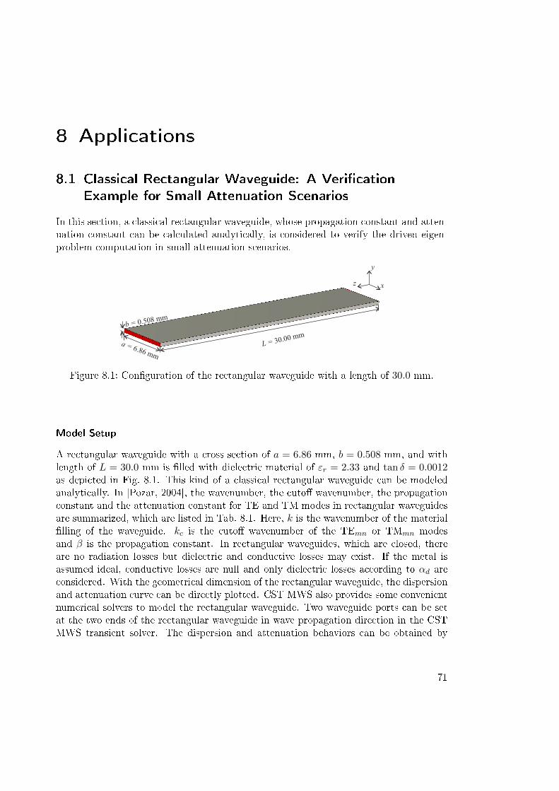
8 Applications
8.1 Classical Rectangular Waveguide: A VericationExample for Small Attenuation Scenarios
In this section, a classical rectangular waveguide, whose propagation constant and atten-uation constant can be calculated analytically, is considered to verify the driven eigen-problem computation in small attenuation scenarios.
a = 6.86 mm
L = 30.00 mm
b = 0.508 mm
z x
y
Figure 8.1: Conguration of the rectangular waveguide with a length of 30.0 mm.
Model Setup
A rectangular waveguide with a cross section of a = 6.86 mm, b = 0.508 mm, and withlength of L = 30.0 mm is lled with dielectric material of εr = 2.33 and tan δ = 0.0012as depicted in Fig. 8.1. This kind of a classical rectangular waveguide can be modeledanalytically. In [Pozar, 2004], the wavenumber, the cuto wavenumber, the propagationconstant and the attenuation constant for TE and TM modes in rectangular waveguidesare summarized, which are listed in Tab. 8.1. Here, k is the wavenumber of the materiallling of the waveguide. kc is the cuto wavenumber of the TEmn or TMmn modesand β is the propagation constant. In rectangular waveguides, which are closed, thereare no radiation losses but dielectric and conductive losses may exist. If the metal isassumed ideal, conductive losses are null and only dielectric losses according to αd areconsidered. With the geometrical dimension of the rectangular waveguide, the dispersionand attenuation curve can be directly plotted. CST MWS also provides some convenientnumerical solvers to model the rectangular waveguide. Two waveguide ports can be setat the two ends of the rectangular waveguide in wave propagation direction in the CSTMWS transient solver. The dispersion and attenuation behaviors can be obtained by
71

8 Applications
monitoring the S-parameters over the ports.
a = 6.86 mm
b = 0.508 mm
l = 2.00 mm
z x
y
port 1
port 2
Figure 8.2: Conguration of the unit cell of the rectangular waveguide with a length of2.00 mm.
Quantity TEmn Mode TMmn Mode
k ω√µε ω
√µε
kc√
(mπ/a)2 + (nπ/b)2√
(mπ/a)2 + (nπ/b)2
β√k2 − k2
c
√k2 − k2
c
αdk2 tan δ
2βk2 tan δ
2β
Table 8.1: Propagation constant and attenuation constant for TE and TM modes inrectangular waveguides.
The rectangular waveguide with the same conguration but modeled as a unit cell witha length of l = 2.00 mm is analyzed with the driven eigenproblem computation method.For a closed waveguide without radiation losses there are only conductive and dielectriclosses both of which are small. Therefore, the perturbation method can be employed toanalyze the attenuation in the rectangular waveguide. As mentioned in section 2.2, thedriven eigenproblem computation is implemented in the CST MWS frequency domainsolver. The unit cell of the rectangular waveguide is discretized with a tetrahedral meshand two discrete ports are placed in the center of it to stimulate and monitor the eld,respectively, as shown in Fig. 8.2. The two ports are placed next to each other in orderto make sure they observe the same eld inside the structure.
72

8.1 Classical Rectangular Waveguide: A Verication Example for Small Attenuation Scenarios
Dispersion and Attenuation Analysis
Fig. 8.3 indicates the perfect agreement among the results from the unit cell employing thedriven method and that from the long length rectangular waveguide using the transientsolver in CST MWS and the analytical method, in both the propagation constant andthe attenuation constant. The blue lines are the dispersion curve which match to eachother perfectly among the three methods. The black lines indicate the dielectric loss ofthe rectangular waveguide which also show great agreement among the results from thethree methods.
14 16 18 20 22 24 260.5
1
1.5
2
2.5
3
3.514 16 18 20 22 24 26
0
100
200
300
400
500
600
700
unit cell with driven method
long length in CST MWS
analytical method [Poz04]
unit cell with driven method
long length in CST MWS
analytical method [Poz04]
frequency [GHz]
atte
nuat
ion c
onst
ant
[Nep
/m]
pro
pag
atio
n c
onst
ant
[m]
-1
frequency [GHz]
Figure 8.3: Propagation and attenuation constants of the rectangular waveguide inFig. 8.1 compared by results from the analytical method, from CST MWSand from the driven method.
73

8 Applications
8.2 Substrate Integrated Waveguide (SIW): Small RadiationExample
Model Setup
An SIW structure as depicted in Fig. 3.7 with geometry parameters d = 0.8 mm, s = 2.0mm, w = 7.2 mm, h = 0.508 mm and lled with a dielectric material of εr = 2.33 andtan δ = 0.0012 is analyzed. The SIW is designed to work at 14− 26 GHz. The bilateralgap s is smaller than λ0
√εr/2, which means the radiation losses from the gap would
be quite small. This makes the SIW a good example for small radiation and can beanalyzed with the driven method with port excitation mentioned in section 5.2. Theunit cell depicted in Fig. 8.4(a) is modeled with the driven method in the frequencysolver of CST MWS.
(a) unit cell of SIW with discrete ports in the center.
(b) SIW with 14 unit cells with waveguide portsat both ends.
Figure 8.4: Geometrical conguration of SIWs. (a) Unit cell of SIW with discrete ports.(b) SIW with 14 unit cells with waveguide ports at both ends in CST MWS
Two discrete ports are set in the center of the unit cell to stimulate the structure andmonitor the resonance behavior, respectively. The periodic boundaries with some phaseshifts are employed in wave propagation direction. By sweeping the frequencies, the reso-nance frequencies can be found for certain phase shifts between the periodic boundaries.The pairs of phase shifts and resonance frequencies form the dispersion curve over a fre-quency range. The perturbation method is employed for the attenuation analysis. The
74

8.2 Substrate Integrated Waveguide (SIW): Small Radiation Example
reference example is an SIW structure with basically the same geometrical parametersbut a longer length of 28 mm depicted in Fig. 8.4(b), which equals to 14 unit cells. Thereference example is analyzed with the transient solver of CST MWS with the waveg-uide ports at both ends. Then, the S-parameter between the two ports are obtained toperform the dispersion and attenuation analysis.
Dispersion and Attenuation Analysis
In the driven method with the discrete ports inside the unit cell, the fundamental mode ofthe resonator can be stimulated. By monitoring the scattering parameters, the resonancefrequency for a certain phase shift between the periodic boundaries, which is alwaysaccompanied with a maximum or a minimum of the scattering matrix, can be foundas shown in Fig. 8.5. It is apparent that |S11|2 + |S21|2 6= 1, which means there aresome losses present in the unit cell resonator. Sweeping the phase dierence between theperiodic boundaries, the corresponding ωres can be found to form the dispersion curve asmentioned in section 5.2 as Eq. (5.2.1). As depicted in Fig. 8.6, for each phase dierence∆ϕ there is only one corresponding resonance frequency ωres which means there is nohigher mode except the fundamental mode TE10 in the operation frequency range.
S1,1
S2,1
frequency [GHz]
Magnitude of S-parameters [dB]
Δφ °=25
Figure 8.5: The scattering parameters of the unit cell depicted in Fig. 8.4(a) with thephase shift ∆ϕ = 25.
The dispersion curve obtained by the driven method with the unit cell agrees excellentlywith the results from CST MWS for the longer SIW as shown in Fig. 8.4(b). Theattenuation constants from the two methods agree with each other also quite well witha trivial deviation which can be reduced by increasing the accuracy of the integration ofthe observable in the perturbation method.
75

8 Applications
Δφ=45 Δφ=50 Δφ=55 Δφ=60 Δφ=65 Δφ=70 Δφ=75Δφ=40Δφ=35Δφ=30Δφ=25Δφ=20
1
0.9
0.8
0.7
0.6
0.5
0.4
0.3
0.2
0.1
015 16 17 18 19 20 21 22 23 24 25
frequency [GHz]
S11
Figure 8.6: Sweeping the phase dierence ∆ϕ to get corresponding resonance frequenciesωres for the SIW unit cell depicted in Fig. 8.4(a).
14 16 18 20 22 24 260.5
0.6
0.7
0.8
0.9
1
1.1
frequency [GHz]
att
en
uati
on
co
nst
an
t[N
ep
/m]
0
100
200
300
400
500
600
700
pro
pag
ati
on
co
nst
an
t[m
-1]
SIW in unit cell,driven eigenproblem computation
SIW 28 mm, with waveguide portin CST MWS
14 16 18 22 24 2620
frequency [GHz]
SIW in unit cell,
driven eigenproblem computation
SIW 28 mm, with waveguide port
in CST MWS
Figure 8.7: Propagation and attenuation constant of the fundamental mode in a SIW inFig. 8.4 computed with driven method and compared with a SIW of lengthof 28 mm with waveguide ports in CST MWS
76

8.3 CRLH Leaky Wave Antenna: Interdigital Design Analysis
8.3 CRLH Leaky Wave Antenna: Interdigital DesignAnalysis
Model Setup
Here a composite right-/left-handed leaky-wave antenna (CRLH LWA) based on a SIWstructure [Weitsch & Eibert, 2010] as depicted in Fig. 8.8 is analyzed by the drivenmethod. The leaky-wave antenna is composed of the unit cell shown in Fig. 8.9 which isrealized on a single-layer printed circuit board (PCB) with a 1.524 mm thick dielectricsubstrate Rogers RO4003 of εr = 3.38 and tan δ = 0.0027. The top copper plate is pe-riodically slotted in an interdigital manner in order to obtain some specic capacitance.The two rows of "teeth" which interdigitate into each other introduce a capacitive gapbetween them. The slots are terminated by two lateral rows of vias and generate anadditional shunt inductance by allowing extra transverse currents.
Figure 8.8: Fabricated CRLH leaky-wave antenna [Weitsch & Eibert, 2010].
Figure 8.9: A unit cell of the CRLH LWA with a periodic length of 5.9 mm[Weitsch & Eibert, 2010].
Dispersion and Attenuation Analysis
Modeling this kind of structure, which has much ner details, e.g. the slot in this ex-ample, compared to the length of the structure will lead to an extremely large numberof mesh cells and an extremely long simulation time if the whole structure is discretizedand analyzed. For example modeling a CRLH LWA with 88.5 mm, which consists of15 unit cells, in the frequency domain solver of CST MWS will generate over 1, 000, 000mesh cells and 2 hours simulation time with a 12-core CPU. However, by employing thedriven method in CST with discrete ports, only one unit cell with 5.9 mm length willbe considered and modeled. This can reduce more than 90% mesh cell and around 75%
77

8 Applications
simulation time. In this CRLH LWA, besides the conductive and dielectric losses thereare also radiation losses. However, the losses are still low which can be analyzed by theperturbation method. Fig. 8.10 depicts the dispersion curves of the CRLH LWA, wherethe results from the driven method, and scattering matrix approach (SMA) as well asmatrix-pencil (MP) method [Weitsch & Eibert, 2010] are compared.
0 20 40 60 80 100 120 1402.5
3
3.5
4
4.5
5
5.5
driven eigenproblem method
MP
SMA with 1 mode
propagation constant [m ]-1
freq
uen
cy [
GH
z]
Figure 8.10: Propagation constant of the CRLH leaky-wave antenna from driven eigen-problem method, Matrix-Pencil (MP), and scattering matrix approach(SMA) [Weitsch & Eibert, 2010].
In Fig. 8.10, a good agreement can be observed among the three sets of data fromdriven method, SMA, and MP. The results from the driven eigenproblem computationin blue shows a bandgap between the left- and right-handed phase constant, which lo-cates between 3.73 GHz and 3.86 GHz. However, the SMA method does not detect thebandgap between the LH and RH which might be caused by the limited mode numberconsidered in the port as mentioned in section 4.3. The driven method can also avoidthe blur in the SMA method around 4.3 GHz which is caused by the cuto frequency ofthe H10-rectangular waveguide mode.
Fig. 8.11 indicates a satisfying agreement between the driven method and measure-ments. Some deviations are due to the fabrication and material tolerance like the under-etching and material inaccuracies. Since the perturbation method is only valid for propa-
78

8.3 CRLH Leaky Wave Antenna: Interdigital Design Analysis
0 5 10 15 20 25 30 353
3.2
3.4
3.6
3.8
4
4.2
4.4
4.6
4.8
5
attenuation constant [Nep/m]
driven eigenproblem method
measurement
freq
uen
cy [
GH
z]
Figure 8.11: Propagation constant of the CRLH leaky-wave antenna from driven eigen-problem method, Matrix-Pencil (MP), and scattering matrix approach(SMA) [Weitsch & Eibert, 2010].
gating waves with relatively small attenuation, it is not possible to compute the attenua-tion constant in the bandgap between 3.73 GHz and 3.86 GHz with this approach in CSTMWS. Therefore, there are deviations between the driven method and the measurementaround the bandgap frequency. This problem can, however, be solved by using the FEBIimplementation where the complex phase shift can be taken into account on the periodicboundary condition. When the evanescent and leaky modes can be described on theboundaries, the attenuation behavior inside the bandgap can be directly calculated.
79

8 Applications
8.4 Periodic Modulated Grounded Dielectric CorrugatedLeaky Wave Antenna: Multi-mode Analysis
8.4.1 Model in 1D Periodic
The periodic modulated grounded dielectric corrugated slab works as an example toverify the FEBI implementation of the driven eigenproblem method. The accelerationmethods mentioned in chapter 6 will be employed to achieve faster convergence in theiteration steps. The periodically modulated grounded dielectric slab is a conventionalwaveguide functioning as a leaky waveguide, which exhibits metamaterial-like behavioron higher space harmonics. With nite width, it has more than one propagation modesin the operating frequency range and it is analyzed to demonstrate the capability of thedriven method in mode selection.
zx
y
p/2
p = 20 mm
3.5 mm
7.0 mm
Figure 8.12: The dielectric corrugated leaky-wave antenna with innite width along thex-axis and its unit cell.
Model Setup
Fig. 8.12 depicts the geometrical conguration of the corrugated dielectric slab working asa leaky wave antenna and the corresponding unit cell. The antenna is designed accordingto the design rule in [Schwering & Peng, 1983] with dielectric substrate Rogers TMM4with relative permittivity εr = 4.5 and tan δ = 0.002 for operation in the frequency range8−14 GHz. Only the wavevector along the coordinate perpendicular to the grooves, herethe y-axis, is considered. The antenna structure and the source distribution are assumeduniform in the coordinate parallel to the grooves, i.e. kx = 0. The unit cell is discretizedin tetrahedra. An impressed volume current density with x-component is applied in someof the tetrahedra as an excitation for TE-modes and the monitored quantity for ndingthe resonance peak is the electric eld in several observation points inside the unit cell.
80

8.4 Periodic Modulated Grounded Dielectric Corrugated LeakyWave Antenna: Multi-mode Analysis
Dispersion and Attenuation Analysis
Fig. 8.13 depicts the reference model using the SMA approach as mentioned in section4.4. The unit cell of the LWA is covered by 6-layer absorbing material with graduallyincreasing thickness and electromagnetic losses to the top in order to reduce the reectionfor the impinging waves. At each port, 8 modes are considered for the modal expansion.Fig. 8.14 demonstrates the comparison of dispersion behaviors between the results fromthe driven method and the results with SMA technique. The light line separates theradiating waves from the purely guided waves. A perfect agreement between the twomethods has been reached. Fig. 8.15 depicts the attenuation behavior of the structure,again the results from the driven method are compared to SMA technique. Some devia-tions are visible, which can probably be attributed to the dierent discretization modelsof the dierent approaches as well as the limited distance between the absorber and theantenna and the limited number of modes considered at each port in SMA. Increasingthe number of the modes considered at each port in SMA, can reduce the deviation asshown in Fig. 8.15. SMA with 8 modes got closer results with the driven method thanthe one with 6 modes. However, it will at the same time increase the simulation timewith SMA.
PEC
PEC
absorbinglayers
port
1
port
2
Figure 8.13: The simulation model in CST MWS for the grounded dielectric corrugatedslab with absorbing layers and 8 modes at each port according to section4.3.
81

8 Applications
0 50 100 150 200 250 300
9.5
10
10.5
11
11.5
12
12.5
13
13.5
14
SMA with 8 modesdriven method
light line
freq
uen
cy [
GH
z]
propagation constant [m ]-1
Figure 8.14: Dispersion diagram of the unit cell according to Fig. 8.12 compared to SMAresults with 8 modes.
0 100 200 300 400 500 600 700 8009
9.5
10
10.5
11
11.5
12
12.5
13
13.5
14
SMA with 8 modes
SMA with 6 modes
driven method
attenuation constant [Nep/m]
freq
uen
cy [
GH
z]
Figure 8.15: Attenuation constant of the unit cell according to Fig. 8.12 compared toSMA results with 6 and 8 modes at ports respectively.
82
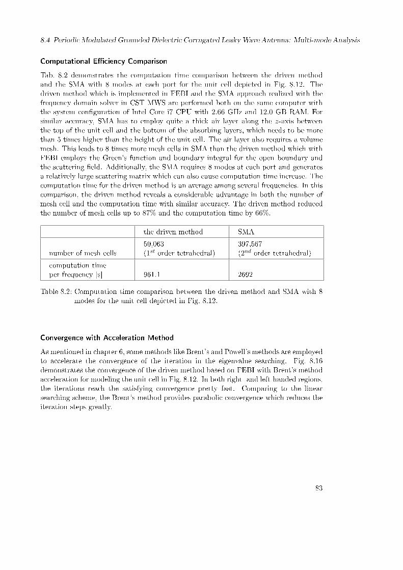
8.4 Periodic Modulated Grounded Dielectric Corrugated LeakyWave Antenna: Multi-mode Analysis
Computational Eciency Comparison
Tab. 8.2 demonstrates the computation time comparison between the driven methodand the SMA with 8 modes at each port for the unit cell depicted in Fig. 8.12. Thedriven method which is implemented in FEBI and the SMA approach realized with thefrequency domain solver in CST MWS are performed both on the same computer withthe system conguration of Intel Core i7 CPU with 2.66 GHz and 12.0 GB RAM. Forsimilar accuracy, SMA has to employ quite a thick air layer along the z-axis betweenthe top of the unit cell and the bottom of the absorbing layers, which needs to be morethan 5 times higher than the height of the unit cell. The air layer also requires a volumemesh. This leads to 8 times more mesh cells in SMA than the driven method which withFEBI employs the Green's function and boundary integral for the open boundary andthe scattering eld. Additionally, the SMA requires 8 modes at each port and generatesa relatively large scattering matrix which can also cause computation time increase. Thecomputation time for the driven method is an average among several frequencies. In thiscomparison, the driven method reveals a considerable advantage in both the number ofmesh cell and the computation time with similar accuracy. The driven method reducedthe number of mesh cells up to 87% and the computation time by 66%.
the driven method SMA
number of mesh cells50,063(1st order tetrahedral)
397,567(2nd order tetrahedral)
computation timeper frequency [s] 961.1 2692
Table 8.2: Computation time comparison between the driven method and SMA with 8modes for the unit cell depicted in Fig. 8.12.
Convergence with Acceleration Method
As mentioned in chapter 6, some methods like Brent's and Powell's methods are employedto accelerate the convergence of the iteration in the eigenvalue searching. Fig. 8.16demonstrates the convergence of the driven method based on FEBI with Brent's methodacceleration for modeling the unit cell in Fig. 8.12. In both right- and left-handed regions,the iterations reach the satisfying convergence pretty fast. Comparing to the linearsearching scheme, the Brent's method provides parabolic convergence which reduces theiteration steps greatly.
83

8 Applications
0 10 20 30 40 50 60-11
-10
-9
-8
-7
-6
-5
-4
-3
-2
-1
iteration steps
f = 9.6 GHz
f = 11.4 GHz
f = 12.0 GHzf = 13.0 GHz
f = 14.0 GHz
rela
tive
resi
dual
[dB
]
Figure 8.16: Convergence of the maximum iterations for the unit cell according toFig. 8.12 at dierent frequencies. The residual is dened with respect tothe accuracy of the complex wavenumber. One iteration corresponds toone parabola evaluation and the iterations are counted independently fromsearch direction.
84

8.4 Periodic Modulated Grounded Dielectric Corrugated LeakyWave Antenna: Multi-mode Analysis
8.4.2 1D Periodic Model with Finite Width
Here the periodic corrugated grounded dielectric slab with nite width of w = 14 mmalong the x-axis, as depicted in Fig. 8.17 is analyzed. Again, in the driven methodthe impressed volume current density is designed to excite the TE modes and only thewavenumber along the y-axis, which is perpendicular to the grooves, is considered. Asreference, the SMA method employs the absorbing layers around the unit cell of the an-tenna to enclose the open conguration, as shown in Fig. 8.18. Therefore, only a limitednumber of modes is sucient to yield accurate results. There are two modes found inthe frequency range of interest, which is 8− 14 GHz.
yz
x
w=
14m
m
7.0m
m
3.5m
m
p/2
p=20 mm
Figure 8.17: The periodic unit cell of the corrugated dielectric LWA with nite width.
PEC
PECPEC
absorbinglayers
PECPEC
Figure 8.18: The CST MWS model for the periodic unit cell of the corrugated dielectricLWA with nite width in SMA with absorbing layers.
85

8 Applications
In Fig. 8.19, a perfect agreement for the propagation constant can be observed betweenthe results from the driven method and the SMA approach with the absorbing layers.There are two modes in the operating frequency range, 8−14 GHz. Both of them exhibitLH and RH behaviors in dierent frequency ranges. The rst mode turns from a LHbehavior into a RH one at 10.45 GHz while the second mode turns at 11.15 GHz.
0 50 100 1508
9
10
11
12
13
14
driven method
SMA
propagation constant [m ]-1
freq
uen
cy [
GH
z]
second mode
first mode
Figure 8.19: Dispersion diagram of the unit cell according to Fig. 8.17 compared to SMAwith 8 modes.
86

8.4 Periodic Modulated Grounded Dielectric Corrugated LeakyWave Antenna: Multi-mode Analysis
For the attenuation constant depicted in Fig. 8.20, the results from the driven methodagree very well with the ones from SMA approach and MP in [Weitsch & Eibert, 2012].For SMA approach the limited air layer height in Fig. 8.18 makes the interference onthe radiation eld distribution between the simulation model and the absorbing layersnot negligible. Also the nite number of modes considered at the ports in SMA mightcontribute to the deviation.
0 2 4 6 8 10 12 148
9
driven method
SMA
MP
attenuation constant [Nep/m]
freq
uen
cy [
GH
z]
Figure 8.20: Attenuation constant of the unit cell according to Fig. 8.17 compared toSMA with 8 modes and matrix pencil (MP) from [Weitsch & Eibert, 2012].
87

8 Applications
Modal Field Solution For Dierent Modes At Dierent Frequencies
The modal eld solution from the driven method can provide a good physical insightinto the structure under analysis as well as it is an excellent tool to distinguish dierentmodes. Fig. 8.21 demonstrates the E-eld distribution at the cross section perpendicularto the wave propagation direction y-axis for the two modes at 13.3 GHz. It is clearlyvisible that there is more energy leaking out to the air for the rst mode than the secondmode at this frequency which also conrms the behavior of the attenuation constant inFig. 8.20. The E-eld distribution for the two modes at another frequency 10.0 GHz isdepicted in Fig. 8.22. According to the attenuation diagram Fig. 8.20, at this frequencythe second mode exhibits more radiation to the free space. The modal eld distributionillustrates the same conclusion.
f = 13.3 GHz
| | in V/mE
1 modest
Air
LWA
(a) rst mode
f = 13.3 GHz
| | in V/mE
2 modend
Air
LWA
(b) second mode
Figure 8.21: Modal eld distribution of the two modes at 13.3 GHz in the port of thecorrugated slab in Fig. 8.17 in xz-plane. (a) rst mode, (b) second mode.
88

8.4 Periodic Modulated Grounded Dielectric Corrugated LeakyWave Antenna: Multi-mode Analysis
(a) first mode
(b) second mode
| in V/m= 10.0 GHz
1 mode
E|f
st
| in V/m= 10.0 GHz
2 mode
E|f
nd
Air
LWA
Air
LWA
Figure 8.22: Modal eld distribution of the two modes at 10.0 GHz in the port of thecorrugated slab in Fig. 8.17 in xz-plane. (a) rst mode, (b) second mode.
89

8 Applications
8.5 Mushroom Structure for MTM: 2D PeriodicConguration
In this section, the mushroom conguration for a 2-dimensional metamaterial is analyzedto demonstrate the performance of the driven method for the 2-dimensional periodicconguration.
top patches
viasground plane
capsh2
h1
(a) (b)
(c)
4.6
4.0
z x
y
Figure 8.23: The mushroom structure [Sanada et al., 2004] and its unit cell. The periodof the unit cell is 5.0 mm × 5.0 mm. The mushroom structure consists of thetop patches and a ground plane which are connected by vias. Between thetop layer and the ground plane there is a dielectric substrate with εr = 2.2and a cap layer under the top patches. (a) Dimensions of the top patchesand the caps in mm. (b) The side view of the mushroom structure. Thedistance between the top patches and the caps is h1 = 0.127 mm and theone between the caps and the ground plane is h2 = 1.697 mm. (c) The unitcell of the mushroom structure.
90

8.5 Mushroom Structure for MTM: 2D Periodic Conguration
Model Setup
As shown in Fig. 8.23, the mushroom structure consists of a layer of top patches andthe ground plane. The top patches are connected to the ground plane by vias of 0.2 mmdiameter. Between the top and the ground metal layers, a dielectric substrate withεr = 2.2 is sandwiched. Under the top patches inside the substrate there is a cap layerto introduce an extra series capacitor. The mushroom structure is periodic in x-andy-direction with the unit cell dimension of 5.0 mm × 5.0 mm. The thickness of the upperand lower substrates are h1 = 0.127 mm and h2 = 1.697 mm, respectively.
Dispersion and Attenuation Analysis
The mushroom structure is a 2D periodic conguration, along both the x- and y-direction.Therefore, the dispersion diagram is a 2D function fn(kx, ky), where n labels the num-ber of the mode. In [Sanada et al., 2004], Brillouin zone and irreducible Brillouin zonewere introduced to demonstrate the dispersion curve for 2D metamaterials. In this work,irreducible Brillouin zone is considered. The dispersion diagrams are computed by thedriven method and compared to the results from [Sanada et al., 2004] obtained by full-wave (FEM) analysis with periodic boundary conditions applied at the edges of the unitcell as depicted in Fig. 8.23(c) along both the x- and y-directions. Fig. 8.24 shows themesh conguration of the mushroom unit cell in Fig. 8.23(c). On the surface, triangu-lar meshes are applied as depicted in Fig. 8.24(b) while in the substrate, the rst ordertetrahedral meshes are employed. In total, 31 193 tetrahedral mesh cells were generatedfor the driven method. The average computation time for one frequency with the drivenmethod was 1 165.5 s. A perfect match can be observed in Fig. 8.25 between the resultsfrom the driven method and the reference [Sanada et al., 2004].
y
x
zx
y
z
(a) The mesh configuration of the mushroom unit cell in Fig. 12(c). (b) The meshes for the top layer, the cap layer and the ground plane.
Figure 8.24: The mesh conguration of the mushroom unit cell.
91

8 Applications
0
5
10
15
20
25
driven methodreference data from[Samada et al., 2004]
Γ ΓΧ Μ
β
f
[GHz]
LH mode
TE mode
RHmode
air
mod
e air mode
Figure 8.25: Dispersion diagrams of the mushroom structure in Fig. 8.23 compared tothe reference data from [Sanada et al., 2004].
Fig. 8.26 and Fig. 8.27 give some examples of modal eld distribution of the mushroomstructure in irreducible Brillouin zone. Fig. 8.26 demonstrates the E-eld distributions ofthe three modes in Γ−X segment of irreducible Brillouin zone. The E-eld distributionson dierent cross sections which belong to one mode are displayed in one column. LHmode at 2.62 GHz is in the rst column, TE mode at 9.11 GHz is in the second column,and in the third column it is RH mode at 14.23 GHz. In each line collect the elddistributions at one cross section. The rst line shows the eld distributions at xy-plane,the second line yz-plane, and the third line zx-plane. The E-eld distributions for RHmode in dierent segments of irreducible Brillouin zone are depicted in Fig. 8.27. TheE-eld distributions at 14.23 GHz in segment Γ−X are in the rst column, the ones at23.68 GHz in X −M are in the second column, and the ones at 13.93 GHz in M −Γ arein the third column.
92

8.5 Mushroom Structure for MTM: 2D Periodic Conguration
LH mode TE mode RH mode
(1a)
(2a)
(3a) (3b) (3c)
(2b) (2c)
(1b) (1c)
Figure 8.26: Modal eld distribution of the three modes of the mushroom structure inFig. 8.23 in Γ−X segment of irreducible Brillouin zone. The rst column isLH mode, the second column is TE mode, the third column is RH mode. (a),(b), and (c) stand for the cross section of xy-, yz-, and zx-plane, respectively.
93

8 Applications
Γ Χ- Μ Γ-Χ Μ-
(3a)
(2a)
(1a) (1b)
(2b)
(3b)
(1c)
(2c)
(3c)
Figure 8.27: Modal eld distribution of the RH modes of the mushroom structure inFig. 8.23 in irreducible Brillouin zone. The rst column is in the segmentΓ−X, the second column is in the segment X −M , the third column is inthe segment M −Γ. (a), (b), and (c) stand for the cross section of xy-, yz-,and zx-plane, respectively.
94

9 Conclusions
The driven eigenproblem computation method opens up a new possibility to solve eigen-problems by solving the corresponding excitation problems in the eigenvalue domain. Itis suitable especially for periodic structures, like metamaterials and substrate integratedwaveguides, which according to Floquet's theorem can be analyzed in an appropriatelydiscretized unit cell with periodic boundary conditions. The unit cell can be analogizedto a resonator in the eigenproblem aspect with the resonance frequencies as eigenvalues.Instead of directly solving the eigenproblem in the resonator as many other eigenproblem-based numerical solvers do, the driven method intends to nd the eigenvalues, here theresonance frequencies, by providing the excitations to the system. Therefore, the sourcefree eigenproblems are transformed into excited eigenvalue problems. Additionally, solv-ing the excitation problem directly in the eigenvalue domain, other than time domainas other excitation algorithms do, can concentrate the energy to an isolated mode andavoid the restrain of limited observation time.
Providing excitations to the system is realized in this work by two methods. Oneis port excitation based on electric circuits and network theory. The other is internal dis-tributed current densities excitation. The port excitation, which couples external energyinto the structure under analysis, is vivid, explicit and compatible with other commer-cial numerical solvers, e.g. CST Microwave Studio, and easy to regularize the resonancebehavior by port impedances. However, the coupling coecient between the excitationports and the structure under analysis will inuence searching of eigenvalues, the res-onance frequencies, through S-parameters. Although this can be solved by monitoringother observables like the elds in the solution domain, its application is sometimes re-stricted to small attenuation scenarios by the limitation in the exibility of the periodicboundary congurations. The perturbation method is employed with the port excitationto analyze the attenuation for guided modes. The attenuation inside the stop band forevanescent and leaky modes can not be analyzed by the perturbation method. On theother hand, the distributed current densities excitation can stimulate in principle all pos-sible modes by electric and magnetic current densities with dierent distributions andpolarizations in the solution domain. With the expectation and understanding of theelds in the solution domain, some specic modes of the elds can be excited by appro-priately designed current densities. Moreover, this kind of excitations has more freedomin eigenvalues searching since some arbitrary observable of the eld solution, such as theelectric eld in the solution domain, or some integral measure of it can be evaluated. Thedistributed current densities excitation is implemented in a hybrid nite element bound-ary integral solver (FEBI). FEBI employs a spectral domain integral equation with aFloquet mode based periodic Green's function interior to the edge-based periodic bound-
95

9 Conclusions
ary condition and the surface integral equation formulations exterior to the boundary forthe scattering and radiation of the open structures. In FEBI, a complex wavevector isallowed in the periodic boundaries and Green's functions, which makes evanescent andleaky modes as well as guided modes analysis possible. Additionally FEBI with dou-bly periodic conguration is more robust in one- and two-dimensional articial materialcompositions like metamaterials.
The eigenvalue (frequency, wavevector) and eigenmodes can fully characterize the prop-erties of a microwave system. Searching the eigenvalues and eigenmodes in an excitedresonator can be realized by monitoring the port S-parameters or the eld quantitiesin the solution domain, which always reach maxima at the resonance frequency. Thismakes the eigenvalue searching in the resonator an optimization procedure. With someinitial estimations based on the previous solutions, the driven method repeats the iter-ations of the solution of the excitation problem with slightly varying parameters. Thiscan be performed by sweeping the frequency with a xed wavevector as well as scanningthe complex plane of the wavevector at a xed frequency, which is more suitable forthe complex modes like evanescent and leaky modes. Some methods like Brent's andPowell's methods are introduced to accelerate the speed of convergence of the searchingiterations. When more than one mode is relevant in the operating frequency range, aglobal optimization is needed to detect all the local extrema corresponding to the dier-ent modes.
The driven method shows the great versatility and accuracy in the dispersion andattenuation analysis of periodic structures. The examples of a classical rectangularwaveguide and a substrate integrated waveguide veries the good accuracy of the drivenmethod compared to analytical methods. In contrast to the scattering matrix approachbased on the modal series expansion, the driven method is more robust and accurate inthe composite right-/left-handed leaky wave antenna example. The periodically modu-lated grounded dielectric corrugated leaky wave antenna examples also demonstrate theeciency of the driven method for one-dimensional open periodic structures where thecomputation consumption and time are greatly reduced while the accuracy is maintainedcompared to the scattering matrix approach. Even with multiple modes operation, thedriven method can still easily distinguish among dierent modes and analyze the modedispersions. A two-dimensional metamaterial based on mushroom structure shows thecapability of the driven method in even more complicated structures.
96

10 Appendix
10.1 General Properties of the Eigenfunctions
Take a wave propagating with a propagation constant β in a waveguide with uniformcross section along the y-axis as an example. The electromagnetic elds for TE, TM, orTEM can be represented as φ(x, z)e−jβy which have to satisfy the Helmholtz equations,
(∇2t + k2
c )φ(x, z) = 0, (10.1.1)
where∇t is a Nabla operator in the transverse plane, here is x−z plane. kc =√k2x + k2
z iscalled cuto wavenumber which is a constant quantity and depends only on the geometryof the guide. Once kc is obtained, the propagation constant β = ky is given by
β = ky =√k2 − k2
c , (10.1.2)
with k = ω√µε the wavenumber of the material lling the transmission line or waveguide
region. Here the function φ(x, z) satisfying (10.1.1) is called the eigenfunction and con-stant kc is the eigenvalue. There can be a set of doubly innite number of eigenfunctions,
φmn, m, n = 0, 1, 2, . . . ,∞, (10.1.3)
according to the dierent boundary conditions, e.g. the Dirichlet's boundary condition
φ(x, z) = 0, on the boundary, (10.1.4)
or the Neumann's boundary condition
∂φ
∂n= 0, on the boundary, (10.1.5)
and with corresponding eigenvalue kmn.
Orthogonality
The eigenfunctions are orthogonal to each other. Consider two eigenfunctions φmn andφm′n′ which both satisfy the wave equations,
(∇2 + k2mn)φmn = 0. (10.1.6)
(∇2 + k2m′n′)φm′n′ = 0. (10.1.7)
97

10 Appendix
Multiply Eq. (10.1.6) with φm′n′ and subtract the result from the multiplication ofEq. (10.1.7) and φmn, we get
φm′n′∇2φmn − φmn∇2φm′n′ = (k2m′n′ − k2
mn)φmnφm′n′ . (10.1.8)
Integrate the both sides of Eq. (10.1.8) and due to the Green's second identity, we canobtain∫
l
(φm′n′
∂φmn∂n
− φmn∂φm′n′
∂n
)dl = (k2
m′n′ − k2mn)
∫sφm′n′φmnds, (10.1.9)
where s is the cross-sectional area, and l is the contour of the cross section. Because φmnand φm′n′ satisfy either the Dirichlet's or the Neumann's boundary condition, the leftside of Eq. (10.1.9) will vanish and it can be rewritten as
(k2m′n′ − k2
mn)
∫sφm′n′φmnds = 0. (10.1.10)
Therefore when m 6= m′ and n 6= n′, kmn 6= km′n′ , the integral in Eq. (10.1.10) must bezero, which can be written as∫
sφmnφm′n′ds = Nmnδmm′δnn′ , (10.1.11)
with
δmm′ =
1 for m = m′
0 for m 6= m′(10.1.12)
and Nmn is the normalizing factor
Nmn =
∫sφ2mnds. (10.1.13)
Completeness
The eigenfunctions form a complete set, with which any continuous function f(r) can beexpanded, as
f(r) =
∞∑m
∞∑n
Amnφmn(r), (10.1.14)
where r = xx+ yy. Amn is the coecient which can be dened as
Amn =
∫s f(r)φmn(r)ds∫s φmn(r)2ds
. (10.1.15)
A delta function δ(r − r′) can also be expressed in a series expansion of eigenfunctions,
δ(r − r′) =∞∑m
∞∑n
φmn(r)φmn(r′)∫s φmn(r)2ds
. (10.1.16)
98

10.2 General Matrix System for CRLH 2D Networks
10.2 General Matrix System for CRLH 2D Networks
Similar to the CRLH 1D network, a general structure of CRLH 2D network as shown inFig. 10.1 with the unit cell as depicted in Fig. 10.2 is considered.
Figure 10.1: A 2D CRLH network consisting of the unit cell depicted in Fig. 10.2 repeatedalong both the x- and y-axis.
The input and output voltages and currents can be related using the transmissionmatrix [ABCD] as shown in Fig. 10.2(b) and thee center node voltage V0 can be obtainedwhen the periodic boundary conditions are applied with periods px and py along the x-and y-axis, respectively [Caloz & Itoh, 2006]
V i0x = V0 =
DixVx −Bi
xIxAixD
ix −Bi
xCix
, (10.2.1)
V i0y = V0 =
DiyVy −Bi
yIy
AiyDiy −Bi
yCiy
, (10.2.2)
V o0x = V0 = (AoxVx +Bo
xIx)e−jkxpx , (10.2.3)
V o0y = V0 = (AoyVy +Bo
yIy)e−jkypy , (10.2.4)
Vsh0 = V0 =
−BshIishAshDsh −BshCsh
, (10.2.5)
(10.2.6)
where kx and ky are the wavenumbers along the x- and y-axis, respectively. Additionally,
99

10 Appendix
(a) The unit cell of the CRLH network in Fig. 10.1.The network is periodic along and y-axis with the periodof and , respectively.
2Dx-
k kx y
(b) The matrix representation of the unit cell. The output currentsand voltages are related to the input currents and voltages by theperiodic boundary conditions. The phase shift can be represented as
= and = where and are the wavenumbers, respectively.φ φx x x y y x yk p k p k ky
Figure 10.2: Unit cell of the 2D CRLH network in Fig. 10.2 [Caloz & Itoh, 2006].
100

10.2 General Matrix System for CRLH 2D Networks
according to Kircho's current law the current for the center node can be obtained as
5∑k=1
Ik =−CixVx +AixIxAixD
ix −Bi
xCix
+−CiyVy +AiyIy
AiyDiy −Bi
yCiy
− (CoxVx +DoxIx)e−jkxpx − (CoyVy +Do
yIy)e−jkypy
+AshI
ish
AshDsh −BshCsh= 0. (10.2.7)
Combining Eq. (10.2.1) to (10.2.5) with (10.2.7) a linear matrix system for the unknownsVx, Ix, Vy, and Iy can be obtain
[M ]
Vx
Ix
Vy
Iy
=
0
0
0
0
, (10.2.8)
where
[M ] =
α− DixAsh
Bsh∆ix
β + BixAshBsh∆i
xγ δ
α β γ − DiyAshBsh∆i
yδ +
BiyAshBsh∆i
y
α− AoxAshexBsh
β − BoxAshexBsh
γ δ
α β γ − AoyAsheyBsh
δ +BoyAsheyBsh
, (10.2.9)
with
α = −Coxex −Cixδix, β = −Do
xex −Aixδix, γ = −Coyey −
Ciyδiy, δ = −Do
yey −Aiyδiy,
(10.2.10)
∆iu = AiuD
iu −Bi
uCiu, (u = x, y), (10.2.11)
ex = e−jkxpx , and ey = e−jkypy . (10.2.12)
This system has a nontrivial solution when
det [M ] = det [M(kx, ky;ω)] = 0. (10.2.13)
When an isotropic network with impedances Z/2 and admittance Y , which is as shownin Fig. 10.2(a), is considered, Eq. (10.2.13) can be simplied after substitution of the
101
10 Appendix
appropriate ABCD parameters [Pozar, 2004]
Aix = Aiy = Aox = Aoy = 1,
Bix = Bi
y = Box = Bo
y = Z/2,
Cix = Ciy = Cox = Coy = 0,
Dix = Di
y = Dox = Do
y = 1,
Ash = 1, Bsh = 0, Csh = Y, Dsh = 1,
∆iu = 1, (u = x, y) (reciprocal network branches). (10.2.14)
After some calculations, we can obtain
(1− e−jkxpx)2
e−jkxpx+
(1− e−jkypy)2
e−jkypy− ZY = 0, (10.2.15)
which can also be written as
2− cos(kxpx)− cos(kypy)−χ
2= 0, (10.2.16)
where χ is dened as
χ = (ω
ωR)2 + (
ωLω
)2 − κω2L, (10.2.17)
ωR =1√
LRCR(rad/s), (10.2.18)
ωL =1√LLCL
(rad/s), (10.2.19)
κ = LRCL + LLCR (s/rad)2. (10.2.20)
Therefore, along the Brillouin zone (BZ) of the periodic lattice, the wavenumbers kx andky can be derived as
Γ−X(0 < kxpx < π, kypy = 0) : kx =1
pxcos−1(1− χ
2), (10.2.21)
X −M(kxpx = π, 0 < kypy < π) : ky =1
pycos−1(3− χ
2), (10.2.22)
M − Γ(0 < kupu < π, u = x, y) : ku =1
pucos−1(1− χ
4). (10.2.23)
10.3 Periodic Green's Function
Consider a periodic structure with period ρa in the x axis and ρb in y axis, and one unitcell dened by 0 < x < ρa, 0 < y < ρb, and −∞ < z < ∞. Within the unit cell, theGreen's function G has to satisfy
(∇2 + k2)G = −δ(x− x′)δ(y − y′)δ(z − z′). (10.3.1)
102

10.3 Periodic Green's Function
Expanding G in the Floquet series,
G =∑m
∑n
gmn(z, z′)e−jkxmx−jkyny, (10.3.2)
where kxm = kx0 + 2mπ/ρa and kym = ky0 + 2nπ/ρb. Substituting Eq. (10.3.2) into(10.3.1) and noting that
δ(x− x′) =∑m
e−jkxm(x−x′)
ρa, (10.3.3)
δ(y − y′) =∑n
e−jkyn(y−y′)
ρb, (10.3.4)
then G can be written as
G =
∞∑m=−∞
∞∑n=−∞
e−jkxm(x−x′)−jkyn(y−y′)
2jkzmn(ρaρb)e−jkzmn|z−z
′|, (10.3.5)
and kzmn = ±√k2
0 − k2xm − k2
yn. If the kxm and kyn are treated as the transverse wavevector ktmn = kt00 + 2π(mρa x+ n
ρby) and consider ρ as the projection of the eld point r
on the xy-plane with r = ρ+ zz, the G can be rewritten as
G(r, r′) =
∞∑m=−∞
∞∑n=−∞
e−jktmn·(ρ−ρ′)
2Ajkzmne−jkzmn|z−z
′|. (10.3.6)
Here A is the area of the cross section of the unit cell's top or bottom boundary surface.
103

List of Figures
3.1 The diagram classies materials in terms of their permittivity ε and per-meability µ. The behavior of a wave incident on the air-material interfacefor each of the possible four cases is shown. The top right quadrant isa conventional dielectric material with positive ε and µ, which shows therefraction with the refraction angle smaller than the incident angle. Themetamaterials in the bottom left quadrant with simultaneously negativeε and µ refract to the same side of the normal indicating reverse Snell'slaw. Plasmas with negative ε and positive µ and microstructured mag-netic materials in the bottom right quadrant with positive ε and negativeµ reect the incident wave. . . . . . . . . . . . . . . . . . . . . . . . . . . 10
3.2 The rst experimental demonstration of negative-ε/negativ-µMTM, com-posed of split-ring resonators with thin wires placed uniformly between them. 11
3.3 Incremental equivalent circuit model for hypothetical uniform LH TL. . . 123.4 Equivalent circuit model for the composite right/left-handed (CRLH) MTMs. 133.5 Balanced and unbalanced CRLH MTMs. . . . . . . . . . . . . . . . . . . . 143.6 Examples of 1D and 2D MTMs. . . . . . . . . . . . . . . . . . . . . . . . . 153.7 The structure of a substrate integrated waveguide by using the metallic
via-hole arrays. . . . . . . . . . . . . . . . . . . . . . . . . . . . . . . . . . 163.8 The structure of a half-mode SIW and the eld distribution [Hong et al., 2006].
(a) The geometrical conguration of a HMSIW. (b) One demonstration ofHMSIW with transition to microstrip line [Hong et al., 2006]. (c) Domaineld distribution in HMSIW [Hong et al., 2006]. . . . . . . . . . . . . . . . 17
3.9 The structure of FSIW. (a) The cross section of a conventional rectangularwaveguide. (b) The cross section of an equivalent folded waveguide. (c)The cross section of an FSIW [Grigoropoulos et al., 2005]. (d) One ex-ample of FSIW with T-septum [Grigoropoulos & Young, 2004]. (e) Oneexample of FSIW without T-septum [Grigoropoulos et al., 2005]. . . . . . 18
3.10 The structure of RSIW [Bao et al., 2012]. . . . . . . . . . . . . . . . . . . 18
4.1 Unit cell of an inhomogeneous periodic structure modeled in the back-ground waveguide with periodic boundaries. . . . . . . . . . . . . . . . . . 28
4.2 The T -matrix connects the modes on the input port to the ones in theoutport of the k-th unit cell. . . . . . . . . . . . . . . . . . . . . . . . . . . 29
4.3 The closed equivalence for an open waveguide structure with PML placedin front of a PEC enclosure. . . . . . . . . . . . . . . . . . . . . . . . . . . 32
4.4 The conguration of absorbing layers. . . . . . . . . . . . . . . . . . . . . 32
105

List of Figures
4.5 A waveguide structure with a uniform cross-section along the y-axis. . . . 354.6 Field distributions for the lower-order modes of a rectangular waveguide
[Pozar, 2004]. . . . . . . . . . . . . . . . . . . . . . . . . . . . . . . . . . . 364.7 Degenerate modes TE11 and TM11 in a rectangular waveguide, which
have both the cuto frequency of 16.145 GHz and propagation constant48.02 per meter but dierent electromagnetic eld distributions. . . . . . . 38
4.8 Mode dispersion of a cylindrical waveguide with a radius of 5 mm andlled with dielectric material with εr = 2.25. Two modes exist in 10-16GHz, one is TE11 with cuto frequency of 11.72 GHz and the other isTM01 with cuto frequency of 15.31 GHz. . . . . . . . . . . . . . . . . . . 39
4.9 The unit cell of the CRLH 2D network in Fig. 3.6 [Caloz & Itoh, 2006]. . . 394.10 Square lattices for a 2D structure. (a) Spatial lattice. (b) Spectral lattice
[Caloz & Itoh, 2006]. . . . . . . . . . . . . . . . . . . . . . . . . . . . . . . 414.11 Dispersion diagram for a 2D balanced CRLH network TL with the param-
eters of Fig. 3.6(b). (a) Conventional representation along the irreducibleBZ. (b) 3D representation of the function fn(kx, ky) (n = 1, 2) over theBZ [Caloz & Itoh, 2006]. . . . . . . . . . . . . . . . . . . . . . . . . . . . . 42
5.1 Basic circuits for shunt and series resonators. . . . . . . . . . . . . . . . . 445.2 Equivalent circuit of the general eigenproblem with port excitation. De-
pendent on the port conguration, a parasitic reactive coupling elementcan be introduced. (b) shows the port voltage applies always on the shuntloss resistor of the virtual resonator, which can be used in loss calculation. 46
5.3 The unit cell of a SIW as depicted in Fig. 3.7 with the port excitation inCST MWS. . . . . . . . . . . . . . . . . . . . . . . . . . . . . . . . . . . . 47
5.4 2D innite periodic conguration. . . . . . . . . . . . . . . . . . . . . . . . 525.5 Conguration of the plane interface. . . . . . . . . . . . . . . . . . . . . . 535.6 The proper Riemann sheet of ky-plane, where Im(kz) < 0. . . . . . . . . . 545.7 The real and complex Floquet modes in the complex transverse wavenum-
ber plane of ky, where Im(kz) < 0 and kx = 0, for the waveguide structureas depicted in Fig. 5.5. . . . . . . . . . . . . . . . . . . . . . . . . . . . . . 55
5.8 The fast and slow wave regions separated by the light line, indicatingradiating waves and purely guided waves. . . . . . . . . . . . . . . . . . . 56
6.1 Magnitude of electric eld at some observation point within the unit cellof a periodic structure at 11.4 GHz over the complex plane of wavenumberky00 = k′y − jk′′y when attenuation is considered. . . . . . . . . . . . . . . . 58
6.2 Inverse parabolic interpolation. . . . . . . . . . . . . . . . . . . . . . . . . 596.3 Golden section search. . . . . . . . . . . . . . . . . . . . . . . . . . . . . . 59
7.1 Resonator coupling methods. (a) electric probe: parallel to the E-eld,(b) current loop: perpendicular to the H-eld, (c) aperture. . . . . . . . . 68
7.2 Rectangular waveguide cavity resonator. . . . . . . . . . . . . . . . . . . . 70
8.1 Conguration of the rectangular waveguide with a length of 30.0 mm. . . 71
106

List of Figures
8.2 Conguration of the unit cell of the rectangular waveguide with a lengthof 2.00 mm. . . . . . . . . . . . . . . . . . . . . . . . . . . . . . . . . . . . 72
8.3 Propagation and attenuation constants of the rectangular waveguide inFig. 8.1 compared by results from the analytical method, from CST MWSand from the driven method. . . . . . . . . . . . . . . . . . . . . . . . . . 73
8.4 Geometrical conguration of SIWs. (a) Unit cell of SIW with discreteports. (b) SIW with 14 unit cells with waveguide ports at both ends inCST MWS . . . . . . . . . . . . . . . . . . . . . . . . . . . . . . . . . . . 74
8.5 The scattering parameters of the unit cell depicted in Fig. 8.4(a) with thephase shift ∆ϕ = 25. . . . . . . . . . . . . . . . . . . . . . . . . . . . . . 75
8.6 Sweeping the phase dierence ∆ϕ to get corresponding resonance frequen-cies ωres for the SIW unit cell depicted in Fig. 8.4(a). . . . . . . . . . . . . 76
8.7 Propagation and attenuation constant of the fundamental mode in a SIWin Fig. 8.4 computed with driven method and compared with a SIW oflength of 28 mm with waveguide ports in CST MWS . . . . . . . . . . . . 76
8.8 Fabricated CRLH leaky-wave antenna [Weitsch & Eibert, 2010]. . . . . . . 778.9 A unit cell of the CRLH LWA [Weitsch & Eibert, 2010]. . . . . . . . . . . 778.10 Propagation constant of the CRLH leaky-wave antenna from driven eigen-
problem method, Matrix-Pencil (MP), and scattering matrix approach(SMA) [Weitsch & Eibert, 2010]. . . . . . . . . . . . . . . . . . . . . . . . 78
8.11 Propagation constant of the CRLH leaky-wave antenna from driven eigen-problem method, Matrix-Pencil (MP), and scattering matrix approach(SMA) [Weitsch & Eibert, 2010]. . . . . . . . . . . . . . . . . . . . . . . . 79
8.12 The dielectric corrugated leaky-wave antenna with innite width along thex-axis and its unit cell. . . . . . . . . . . . . . . . . . . . . . . . . . . . . . 80
8.13 The simulation model in CST MWS for the grounded dielectric corrugatedslab with absorbing layers and 8 modes at each port according to section4.3. . . . . . . . . . . . . . . . . . . . . . . . . . . . . . . . . . . . . . . . . 82
8.14 Dispersion diagram of the unit cell according to Fig. 8.12 compared toSMA results with 8 modes. . . . . . . . . . . . . . . . . . . . . . . . . . . 83
8.15 Attenuation constant of the unit cell according to Fig. 8.12 compared toSMA results with 6 and 8 modes at ports respectively. . . . . . . . . . . . 83
8.16 Convergence of the maximum iterations for the unit cell according toFig. 8.12 at dierent frequencies. The residual is dened with respectto the accuracy of the complex wavenumber. One iteration correspondsto one parabola evaluation and the iterations are counted independentlyfrom search direction. . . . . . . . . . . . . . . . . . . . . . . . . . . . . . 85
8.17 The periodic unit cell of the corrugated dielectric LWA with nite width. . 868.18 The CST MWS model for the periodic unit cell of the corrugated dielectric
LWA with nite width in SMA with absorbing layers. . . . . . . . . . . . . 868.19 Dispersion diagram of the unit cell according to Fig. 8.17 compared to
SMA with 8 modes. . . . . . . . . . . . . . . . . . . . . . . . . . . . . . . 878.20 Attenuation constant of the unit cell according to Fig. 8.17 compared to
SMA with 8 modes and matrix pencil (MP) from [Weitsch & Eibert, 2012]. 88
107
List of Figures
8.21 Modal eld distribution of the two modes at 13.3 GHz in the port of thecorrugated slab in Fig. 8.17 in xz-plane. (a) rst mode, (b) second mode. 89
8.22 Modal eld distribution of the two modes at 10.0 GHz in the port of thecorrugated slab in Fig. 8.17 in xz-plane. (a) rst mode, (b) second mode. 90
8.23 The mushroom structure [Sanada et al., 2004] and its unit cell. The periodof the unit cell is 5.0 mm × 5.0 mm. The mushroom structure consists ofthe top patches and a ground plane which are connected by vias. Betweenthe top layer and the ground plane there is a dielectric substrate withεr = 2.2 and a cap layer under the top patches. (a) Dimensions of the toppatches and the caps in mm. (b) The side view of the mushroom structure.The distance between the top patches and the caps is h1 = 0.127 mm andthe one between the caps and the ground plane is h2 = 1.697 mm. (c)The unit cell of the mushroom structure. . . . . . . . . . . . . . . . . . . . 91
8.24 The mesh conguration of the mushroom unit cell. . . . . . . . . . . . . . 928.25 Dispersion diagrams of the mushroom structure in Fig. 8.23 compared to
the reference data from [Sanada et al., 2004]. . . . . . . . . . . . . . . . . 938.26 Modal eld distribution of the three modes of the mushroom structure
in Fig. 8.23 in Γ − X segment of irreducible Brillouin zone. The rstcolumn is LH mode, the second column is TE mode, the third column isRH mode. (a), (b), and (c) stand for the cross section of xy-, yz-, andzx-plane, respectively. . . . . . . . . . . . . . . . . . . . . . . . . . . . . . 94
8.27 Modal eld distribution of the RH modes of the mushroom structure inFig. 8.23 in irreducible Brillouin zone. The rst column is in the segmentΓ−X, the second column is in the segment X −M , the third column isin the segment M −Γ. (a), (b), and (c) stand for the cross section of xy-,yz-, and zx-plane, respectively. . . . . . . . . . . . . . . . . . . . . . . . . 95
10.1 A 2D CRLH network consisting of the unit cell depicted in Fig. 10.2 re-peated along both the x- and y-axis. . . . . . . . . . . . . . . . . . . . . . 101
10.2 Unit cell of the 2D CRLH network in Fig. 10.2 [Caloz & Itoh, 2006]. . . . 102
108
Bibliography
[Abramowitz & Stegun, 1984] Abramowitz, M. & Stegun, I. A. (1984). Pocketbook ofMathematical Functions. Frankfurt am Main: Verlag Harri Deutsch.
[Akhmanov & Nikitin, 1997] Akhmanov, A. & Nikitin, S. Y. (1997). Physical Optics.Oxford University Press.
[Asvestas, 1980] Asvestas, J. S. (1980). The physical optics method in electromagneticscattering. Journal of Mathematical Physics, 21(2), 290299.
[Baba, 1981] Baba, N. (1981). Convergence of a random optimization method for con-strained optimizations problems. Journal of Optimization Theory and Applications,33(4), 451461.
[Bahl & Bhartia, 2003] Bahl, I. & Bhartia, P. (2003). Microwave Solid State CircuitDesign. Wiley-Interscience, second edition.
[Bao et al., 2012] Bao, J., Tong, C., Zou, X., & Yu, D. (2012). Ridged substrate inte-grated waveguide. In International Conference on Microwave and Millimeter WaveTechnology (ICMMT), volume 2 (pp. 14).
[Basu et al., 2006] Basu, S., Pollack, R., & Roy, M. (2006). Algorithms in Real AlgebraicGeometry. Berlin: Springer.
[Baum et al., 1991] Baum, C. E., Rothwell, E. J., Chen, K.-M., & Nyquist, D. P. (1991).The singularity expansion method and its application to target identication. Proceed-ing of the IEEE, 79(10), 14811492.
[Bérenger, 1994] Bérenger, J. P. (1994). A perfectly matched layer for the absorption ofelectromagnetic waves. Journal of Computational Physics, 114(2), 185200.
[Bondeson et al., 2005] Bondeson, A., Rylander, T., & Ingelstrom, P. (2005). Computa-tional Electromagnetics. New York: Springer Science.
[Bozzi et al., 2006] Bozzi, M., Perregeini, L., & Wu, K. (2006). Direct determination ofmulti-mode equivalent circuit models for discontinuities in substrate integrated waveg-uide. In 2006 IEEE MTT-S International Microwave Symposium Digest, June 1116,San Francisco, USA (pp. 6871).
[Bozzi et al., 2009] Bozzi, M., Rerregrini, L., Wu, K., & Arcioni, P. (2009). Current andfuture research trends in substrate integraged waveguide technology. Radioengineering,18(2), 201208.
109

Bibliography
[Brent, 2002] Brent, R. P. (2002). Algorithms for Minimization without Derivatives.Englewood Clis, Prentice Hall.
[Caloz & Itoh, 2002] Caloz, C. & Itoh, T. (2002). Application of the transmission linetheory of left-handed (LH) materials to the realization of a microstrip lh transmis-sion line. In Progress in IEEE International Symposium on Antenna and Propagationand USNC/URSI National Radio Science Meeting, June 2002, San Antonio, USA,volume 52 (pp. 412415).
[Caloz & Itoh, 2003] Caloz, C. & Itoh, T. (2003). Novel microwave devices and structuresbased on the transmission line approach of meta-materials. In 2003 IEEE MTT-SInternational Microwave Symposium Digest, June 813, Philadelphia, USA, volume 1(pp. 195198).
[Caloz & Itoh, 2006] Caloz, C. & Itoh, T. (2006). Electromagnetic Metamaterials: Trans-mission Line Theory and Microwave Applications. New Jersey: Wiley-interscience.
[Cassivi et al., 2002] Cassivi, Y., Perregrini, L., Arcioni, P., Wu, K., & Conciauro, G.(2002). Dispersion characteristics of substrate integrated rectangular waveguide. IEEEMicrowave and Wirless Components Letters, 12(9), 333335.
[Cesari & Abel, 1972] Cesari, C. S. & Abel, J. F. (1972). Introduction to the FiniteElement Method: a Numerical Approach for Engineering Analysis. New York: VanNostrand Reinhold.
[Chen et al., 1988] Chen, G. L., Owens, T. L., & Whealton, J. H. (1988). Theoreticalstudy of the folded waveguide. IEEE Trans. Plasma Sci., 16(2), 305311.
[Chen et al., 2011] Chen, H., Schmidt, C. H., Che, W., & Eibert, T. F. (2011). Dispersionand attenuation analysis of substrate integrated waveguide by driven eigenproblemcompuation. In European Conference on Antenna and Propagation (EuCAP), April2011, Rome, Italy (pp. 643646).
[Collin, 1991] Collin, R. E. (1991). Field Theory of Guided Waves. New York: IEEEPress.
[CST, 2011] CST (2011). 3d em eld simulation mws microwave studio - cst computersimulation technology. http://www.cst.com.
[Davidson, 2005] Davidson, D. B. (2005). Computational Electromagnetics for RF andMicrowave Engineering. Cambridge, UK: Cambridge University Press.
[Derudder et al., 1998] Derudder, H., de Zutter, D., & Olyslager, F. (1998). Analysisof waveguide discontinuities using perfectly matched layers. Electronics Lett., 34(2),213852140.
[Derudder et al., 2001] Derudder, H., Olyslager, F., de Zutter, D., & van den Berghe, S.(2001). Ecient mode-matching analysis of discontinuities in nite planar subsrates
110

Bibliography
using perfectly matched layers. IEEE Transactions on Antennas and Propagation,49(2), 185195.
[Deslandes & Wu, 2006] Deslandes, D. & Wu, K. (2006). Accurate modeling, wavemechanisms, and design considerations of a substrate integrated waveguide. In 2002IEEE MTT-S International Microwave Symposium Digest, June 26, Seattle, USA,volume 54.
[Duran & Grossmann, 1986] Duran, M. A. & Grossmann, I. E. (1986). An outer-approximation algorithm for a class of mixed-integer nonlinear programs. MathmaticalProgramming, 36, 307339.
[Earl & Deem, 2005] Earl, D. J. & Deem, M. W. (2005). Parallel tempering: theory,applications, and new perspectives. Physical Chemistry Chemical Physics, 7, 39103916.
[Eibert et al., 2011] Eibert, T., Weitsch, Y., & Chen, H. (2011). Dispersion analysisof periodic structures by solving corresponding excitation problems. In German Mi-crowave Conference (GeMIC) (pp. 14). Darmstadt, Germany.
[Eibert et al., 2003] Eibert, T. F., Erdemli, Y. E., & Volakis, J. L. (2003). Hybrid niteelement-fast spectral domain multilayer boundary integral modeling of doubly periodicstructures. IEEE Transactions on Antennas and Propagation, 51(9), 25172520.
[Eibert et al., 1999] Eibert, T. F., Volakis, J. L., Wilton, D. R., & Jackson, D. R. (1999).Hybrid FE/BI modeling of 3D doubly periodic structures utilizing triangular prismaticelements and a MPIE formulation accelerated by the Ewald transformation. IEEETransactions on Antennas and Propagation, 47(5), 843850.
[Eibert et al., 2012] Eibert, T. F., Weitsch, Y., Chen, H., & Gruber, M. E. (2012). Solv-ing periodic eigenproblems by solving corresponding excitation problems in the domainof the eigenvalue. Progress in Electromagnetics Research, 126, 6584.
[Felsen & Marcuvitz, 1994] Felsen, L. B. & Marcuvitz, N. (1994). Radiation and Scat-tering of Waves. IEEE Press.
[Garcia & Gould, 1980] Garcia, C. B. & Gould, F. J. (1980). Relations between severalpath-following algorithms and local and global newton methods. SIAM Review, 22(3),263274.
[Grbic & Eleftheriades, 2002] Grbic, A. & Eleftheriades, G. V. (2002). A backward-waveantenna base on negative refractive index L-C network. In Progress in IEEE Inter-national Symposium on Antenna and Propagation and USNC/URSI National RadioScience Meeting, June 2002, San Antonio, USA, volume 4 (pp. 340343).
[Greivenkamp, 2004] Greivenkamp, J. E. (2004). Field Guide to Geometrical Optics.SPIE Press Book.
111

Bibliography
[Grigoropoulos et al., 2005] Grigoropoulos, N., Sanz-Izquierdo, B., & Young, P. R.(2005). Substrate integrated folded waveguides (SIFW) and lters. IEEE MicrowaveWireless Compon. Lett., 15(12), 829831.
[Grigoropoulos & Young, 2004] Grigoropoulos, N. & Young, P. R. (2004). Compactfolded waveguides. In 34th European Microwave Conference, Amsterdam, Holland,12.14.10.2004 (pp. 973976).
[Guru & Hiziroglu, 2004] Guru, B. S. & Hiziroglu, H. R. (2004). Electromagnetic FieldTheory Fundamentals. Cambridge Unveristy Press, second edition.
[Hamacher, 2006] Hamacher, K. (2006). Adaptation in stochastic tunneling global opti-mization of complex potential energy landscapes. Europhysics Letters, 74(6), 944.
[Hamacher & Wenzel, 1999] Hamacher, K. & Wenzel, W. (1999). The scaling behaviourof stochastic minimization algorithms in a perfect funnel landscape. Physical ReviewE, 59(1), 938941.
[Harrington, 1968] Harrington, R. F. (1968). Field Computation by Moment Methods.New York: The Macmillan Co.
[Heaviside, 1888] Heaviside, O. (1888). On electromagnetic waves, especially in relationto the vorticity of the impressed forces, and the forced vibration of electormagneticsystems. Philosophical Magazine, 25, 130156.
[Hong et al., 2006] Hong, W., Liu, B., Wang, Y., Lai, Q., Tang, H., Yin, X., Dong, Y.,Zhang, Y., & Wu, K. (2006). A new guided wave structure for microwave and millime-ter wave application. Joint 31st International Conference on Infrared and MillimeterWaves and 14th International Conference on Terahertz Electronics, (pp. 1822).
[Hopfer, 1955] Hopfer, S. (1955). The design of ridged waveguides. IRE Transactions onMicrowave Theory and Techniques, 10, 2029.
[Ishimaru, 1991] Ishimaru, A. (1991). Electromagnetic Wave Propagation, Radiation,and Scattering. ISBN 0-13-249053-6. Prentice Hall.
[IYER & Eleftheriades, 2002] IYER, A. K. & Eleftheriades, G. V. (2002). Negative re-fractive index metamaterials supporting 2-D waves. In 2002 IEEE MTT-S Interna-tional Microwave Symposium Digest, June 26, Seattle, USA, volume 2 (pp. 412415).
[Jibetean & de Klerk, 2006] Jibetean, D. & de Klerk, E. (2006). Global Optimization ofRational Functions: A Semidenite Programming Approach. Open Access publicationsfrom Tilburg University urn:nbn:nl:ui:12-174725, Tilburg University.
[Jin, 2002] Jin, J. (2002). The Finite Element Method in Electromagnetics. New York:John Wiley & Sons, Inc.
[Kalos & Whitlock, 2008] Kalos, M. H. & Whitlock, P. A. (2008). Monte Carlo Methods.Wiley-VCH.
112
Bibliography
[Karageorchis, 2001] Karageorchis, A. (2001). The method of fundamental solutions forthe calculation of the eigenvalues of the Helmholtz equation. Applied MathematicsLetters, 14, 837842.
[Kavasseri, 2007] Kavasseri, R. G. (2007). A computational algegraic geometry basedglobal optimization technique to address economic dispatch. In IEEE Power Engi-neering Society General Meeting (pp. 18).
[Keller, 1987] Keller, H. B. (1987). Lectures on Numerical Methods in Bifurcation Prob-lems. Heidelberg, Germany: Springer Verlag.
[Keller, 1962] Keller, J. B. (1962). Geometrical theory of diraction. Journal of theOptical Society of America, 52(2), 116130.
[Kirkpatrick et al., 1983] Kirkpatrick, S., Gelatt, C. D., & Vecchi, M. P. (1983). Opti-mization by simulated annealing. Science, 220(4598), 671680.
[Kitagawa, 1988] Kitagawa, T. (1988). On the numerical stability of the method offundamental solution applied to the Dirichlet problem. Applied Mathematics Letters,5, 123133.
[Kitagawa, 1991] Kitagawa, T. (1991). Asymptotic stability of the fundamental solutionmethod. Journal of Computaional and Applied Mathematics, 38, 263269.
[Kittel, 1964] Kittel, C. (1964). Introduction to Solid State Physics. Wiley Text Books,seventh edition.
[Kong, 2009] Kong, J. A. (2009). Electromagnetic Wave Theory. New York, USA: WileyInterscience, second edition.
[Kurokawa, 1958] Kurokawa, K. (1958). The expansions of electromagnetic elds in cav-ities. IRE Trans. Microwave Theory Tech., MTT-6, 178187.
[Liberti, 2008] Liberti, L. (2008). Introduction to Global Optimization. Online availableat http://www.lix.polytechnique.fr/ liberti/teaching/globalopt-lima.pdf.
[Lu & Chew, 1995] Lu, C. C. & Chew, W. C. (1995). The use of Huygens' equivalenceprinciple for solving 3D volume integral equation of scattering. IEEE Transactions onAntennas and Propagation, 43(5), 500507.
[Luan & Tan, 2011] Luan, X. & Tan, K. (2011). A novel ridge substrate integratedwaveguide antenna for WLAN application. In International Workshop on AntennaTechnology (iWAT) (pp. 302305).
[Luan & Tan, 2012] Luan, X. & Tan, K. (2012). Ultra-wideband bandpass lter basedon ridged substrate integrated waveguide. In International Conference on Microwaveand Millimeter Wave Technology (ICMMT), volume 4 (pp. 14).
113

Bibliography
[Matyas, 1965] Matyas, J. (1965). Random optimization. Automation and Remote Con-trol, 26(2), 246253.
[Maxwell, 1873] Maxwell, J. C. (1873). Treatise on Electricity and Magnetism. Oxford:Clarendon Press.
[Metropolis & Ulam, 1949] Metropolis, N. & Ulam, S. (1949). The Monte Carlo method.Journal of the American Statistical Association, 44(247), 335341.
[Michalski, 1985] Michalski, K. A. (1985). On the ecient evaluation of integrals arisingin the Sommerfeld halfspace problem. IEE Proceedings H, Microwaves, Antennas andPropagation, 132(5), 312318.
[Oliner, 2003] Oliner, A. A. (2003). A planar negative-refractive-index medium withoutresonant elements. In 2003 IEEE MTT-S International Microwave Symposium Digest,June 813, Philadelphia, USA, volume 1 (pp. 191194).
[Pendry et al., 1998] Pendry, J. B., Holden, A. J., Robbins, D. J., & Stewart, W. J.(1998). Low frequency plasmons in thin-wire structures. Journal of Physics: Con-densed Matter, 10, 47854809.
[Pendry et al., 1999] Pendry, J. B., Holden, A. J., & Stewart, W. J. (1999). Magnetismfrom conductors and enhanced nonlinear phenomena. IEEE Transactions on Mi-crowave Theory and Techniques, 47(11), 20752084.
[Pendry et al., 1996] Pendry, J. B., Holden, A. J., Stewart, W. J., & Youngs, I. (1996).Extremely low frequency plasmons in metallic mesostructure. Physical Review Letters,76(25), 47734776.
[Pozar, 2004] Pozar, D. M. (2004). Microwave Engineering. Hoboken: Wiley.
[Russer, 2006] Russer, P. (2006). Electromagnetics, Microwave Circuit and Antenna De-sign for Communications Engineering. Artech House, second edition.
[Sanada et al., 2004] Sanada, A., Caloz, C., & Itoh, T. (2004). Planar distributed struc-tures with negative refractive index. IEEE Transactions on Microwave Theory andTechniques, 52(4), 12521263.
[Schuhmann et al., 2005] Schuhmann, R., Lubkowski, G., & Weiland, T. (2005). Full-wave simulations and extraction of eective material parameters for left-handed meta-materials. In German Microwave Conference (GeMIC) Ulm, Germany.
[Schuster, 1904] Schuster, A. (1904). An Introduction to the Theory of Optics. London:Edward Arnold.
[Schwering & Peng, 1983] Schwering, F. K. & Peng, S. T. (1983). Design of dielectricgrating antennas for millimeter-wave applications. IEEE Transactions on MicrowaveTheory and Techniques, 31(2), 199209.
114

Bibliography
[Sievenpiper et al., 1999] Sievenpiper, D., Zhang, L., Broas, R. F. J., Alexopolous, N. G.,& Yablonovitch, E. (1999). High-impedance surface electromagnetic surfaces with aforbidden frequency band. IEEE Transactions on Microwave Theory and Techniques,47(11), 20592074.
[Smith et al., 2000] Smith, D. R., Padilla, W. J., Vier, D., Nemat-Nasser, S., & Schultz,S. (2000). Composit medium with simultaneously negative permeability and permit-tivity. Physical Review Letters, 84(18), 4184.
[Sommerfeld, 1949] Sommerfeld, A. (1949). Partial Dierential Equations in Physics.Academic Press.
[Swendsen & Wang, 1986] Swendsen, R. H. & Wang, J. S. (1986). Replica Monte Carlosimulation of spin glasses. Physical Review Letters, 57, 26072609.
[Tamir & Oliner, 1963] Tamir, T. & Oliner, A. A. (1963). Guided complex waves. part1: Fields at an interface. Proceeding of the IEE, 110(2), 310324.
[Teixeira & Chew, 1996] Teixeira, F. L. & Chew, W. C. (1996). PML-FDTD in cylin-drical and spherical grids. IEEE Microwave and Guided Wave Lett., 7, 285287.
[Tuy, 1998] Tuy, H. (1998). Conves Analysis and Global Optimization. Dodrecht: KluwerAcademic Publishers.
[Umtsev, 2007] Umtsev, P. Y. (2007). Fundamentals of the Physical Theory of Dirac-tion. Wiley-IEEE Press, rst edition.
[erný, 1985] erný, V. (1985). Thermodynamical approach ot the traveling salesmanproblem: an ecient simulation algorithm. Journal of Optimization Theory and Ap-plications, 45, 4151.
[Veselago, 1968] Veselago, V. G. (1968). The electrodynamics of substances with simul-taneously negative values of ε and µ. Physics-Uspekhi, 10(4), 509514.
[Weise, 2008] Weise, T. (2008). Global Optimization Algorithms Theory and Application.Self-Published, second edition. Online available at http://www.it-weise.de/.
[Weitsch et al., 2011] Weitsch, Y., Chen, H., & Eibert, T. F. (2011). Dispersion analysisof periodic structures by solving corresponding excitation problems. Frequenz, 65(7-8),247252.
[Weitsch & Eibert, 2010] Weitsch, Y. & Eibert, T. F. (2010). Composite right-/left-handed interdigital leaky-wave antenna on a substrate integrated waveguide. In Eu-ropean Conference on Antenna and Propagation (EuCAP), April 2010, Barcelona,Spain.
[Weitsch & Eibert, 2011] Weitsch, Y. & Eibert, T. F. (2011). Eigenvalue computationof open periodically composed waveguides by series expansion. In Progress in IEEE
115

Bibliography
Antennas and Propagation Society International Symposium, July 2011, Spokane, WA,USA (pp. 321324).
[Weitsch & Eibert, 2012] Weitsch, Y. & Eibert, T. F. (2012). Modal series expansionof eigensolutions for closed and open periodic waveguides. IEEE Transactions onAntennas and Propagation, 60(12), 58815889.
[Xu et al., 2006] Xu, F., Wu, K., & Hong, W. (2006). Domain decomposition FDTDalgorithm combined with numerical tl calibration technique and its application in pa-rameter extraction of substrate integrated circuits. IEEE Transactions on MicrowaveTheory and Techniques, 54(1), 329338.
[Xu et al., 2007] Xu, F., Wu, K., & Hong, W. (2007). Finite-dierence time-domainmodeling of periodic guided-wave structures and its application to the analysis of sub-strate integrated nonradiative dielectric waveguide. IEEE Transactions on MicrowaveTheory and Techniques, 55(12), 25022511.
[Xu et al., 2003] Xu, F., Zhang, Y., Hong, W., Wu, K., & Cui, T. J. (2003). Finite-dierence frequency-domain algorithm for modeling guided-wave properties of sub-strate integrated waveguide. IEEE Transactions on Microwave Theory and Techniques,51(11), 22212227.
[Yang & Beck, 1998] Yang, C. M. & Beck, J. L. (1998). Generalized trajectory methodsfor nding multiple extrema and roots of functions. Journal of Optimization Theoryan Applications, 97(1), 211227.
[Yee, 1966] Yee, K. S. (1966). Numerical solution of initial boundary value problemsinvolving Maxwell's equations. IEEE Transactions on Antennas and Propagation,14(3), 302307.
116


![SPONGE: A generalized eigenproblem for clustering signed ...cucuring/signedClustering.pdf · Spectral methods on signed networks began with Anchurietal. [5],whoseproposedapproachoptimizes](https://static.fdocuments.in/doc/165x107/5f757f10da94a93a6930a0c0/sponge-a-generalized-eigenproblem-for-clustering-signed-cucuring-spectral.jpg)