NASA/CR- 1998-208746

ICASE Report No. 98-52

Global Artificial Boundary Conditions for

Computation of External Flow Problems with

Propulsive Jets

Semyon Tsynkov and Saul Abarbanel

Tel Aviv University, Tel Aviv, Israel

Jan Nordstr6m

The Aeronautical Research Institute of Sweden, Bromma, Sweden

Viktor Ryaben 'kii

Russian Academy of Sciences, Moscow, Russia

Veer Vatsa

NASA Langley Research Center, Hampton, Virginia

Institute for Computer Applications in Science and Engineering

NASA Langley Research Center, Hampton, VA

Operated by Universities Space Research Association

National Aeronautics andSpace Administration

Langley Research CenterHampton, Virginia 23681-2199

Prepared for Langley Research Centerunder Contract NAS 1-97046

November 1998

https://ntrs.nasa.gov/search.jsp?R=19990014059 2018-06-26T19:19:39+00:00Z

Available from the following:

NASA Center for AeroSpace Information (CASI)

7121 Standard Drive

Hanover, MD 21076-1320

(301) 621-0390

National Technical Inf_rmation Service (NTIS)5285 Port Royal Road

Springfield, VA 22161-2171

(703) 487-4650

GLOBAL ARTIFICIAL BOUNDARY CONDITIONS FOR COMPUTATION OF

EXTERNAL FLOW PROBLEMS WITH PROPULSIVE JETS*

SEMYON TSYNKOV t, SAUL ABARBANEL_, JAN NORDSTROM§, VIKTOR RYABEN'KII ¶, AND VEER VATSAdl

Abstract. We propose new global artificial boundary conditions (ABC's) for computation of flows

with propulsive jets. The algorithm is based on application of the difference potentials method (DPM).

Previously, similar boundary conditions have been implemented for calculation of external compressible

viscous flows around finite bodies. The proposed modification substantially extends the applicability range

of the DPM-based algorithm. In the paper, we present the general formulation of the problem, describe our

numerical methodology, and discuss the corresponding computational results. The particular configuration

that we analyze is a slender three-dimensional body with boat-tail geometry and supersonic jet exhaust in

a subsonic external flow under zero angle of attack. Similarly to the results obtained earlier for the flows

around airfoils and wings, current results for the jet flow case corroborate the superiority of the DPM-based

ABC's over standard local methodologies from the standpoints of accuracy, overall numerical performance,

and robustness.

Key words, external flow problems, jet exhaust, artificial boundary conditions, difference partials

method

Subject classification. Applied and Numerical Mathematics

1. Introduction. Many typical problems in aerodynamics including those that present immediate

practical interest, e.g., flows around aircraft, are formulated on infinite domains. It is, however, obvious,

that any discretization used for solving such problems on the computer must be finite. Therefore, any

numerical solution methodology for these problems has to bc supplemented (or, rather, preceded) by a

special technique that helps create such finite discretizations.

A widely used approach to this problem is based on truncating the original flow domain prior to the

actual discretization and numerical solution. Subsequently, one can construct a finite discretization on the

new bounded computational domain using one of the standard techniques: finite differences, finite elements,

or other. However, both the continuous problem on the truncated domain and its discrete counterpart

will be subdefinite unless supplemented by the appropriate closing procedure at the external computational

boundary. This is done by using artificial boundary conditions (ABC's); the word "artificial" emphasizing

here that these boundary conditions are necessitated by numerics and do not come from the original physical

formulation.

The ideal or, in other words, exact, ABC's are obviously those that would drive the error associated

*This research was supported by the Director's Discretionary Fund and the National Aeronautics and Space Administration

under NASA Contract No. NAS1-97046 while the first through fourth authors were in residence at the Institute for Computer

Applications in Science and Engineering (ICASE), NASA Langley Research Center, Hampton, VA 23681-2199.

t School of Mathematical Sciences, Tel Aviv University, Ramat Aviv, Tel Aviv 69978, Israel, tsy_kov_nath, tau. ac. il.

*School of Mathematical Sciences, Tel Aviv University, Ramat Aviv, Tel Aviv 69978, Israel, saul_nath.tau, ac. il.

§FFA, The Aeronautical Research Institute of Sweden, Box 11021, S-161 11, Bromma, Sweden, nmj@ffa, se.

_IKeldysh Institute for Applied Mathematics, Russian Academy of Sciences, 4 Miusskaya Sq., Moscow 125047, Russia,

ryab@spp,keldysh,ru.

IIAerodynamic and Acoustic Methods Branch, Fluid Mechanics and Acoustics Division, Mail Stop 128, NASA Langley

Research Center, Hampton, VA 23681-2199, vatsa@tabdemo.laxc.nasa.gov.

with domain truncation to zero. However, numerically efficient procedures of this kind cannot bc attained

routinely except in model (mostly one-dimensional) problems and therefore, for typical applications one uses

primarily different approximate rather than exact methodological.

The nature of the difficulties associated with constructing _he exact ABC's is that in most cases such

boundary conditions appear nonlocal (in space and also in time for unsteady problems). Although the cor-

responding computational algorithms are robust and highly accurate, they can be cumbersome and typically

apply only to rather simple geometries. On the other hand, _he alternative local approaches that yield

inexpensive and geometrically universal numerical procedures may often lack accuracy in computations,

which, in turn, necessitates choosing excessively large computational domains. Basically, higher accuracy

due to boundary conditions implies that more of the nonlocal nature of exact ABC's has to be taken into

consideration. As a consequence, to avoid extra complexity due to the nonlocality of boundary conditions,

most of the modern production algorithms in CFD still employ local ABC's that arc based on simplified

flow models. The possibility to use local ABC's comes, as mcnl;ioned, at the expense of running the cases

on large domains.

Generally, it has been demonstrated theoretically and comp,atationally in both CFD and other areas of

scientific computing that the treatment of ABC's may have a profound impact on the overall performance

of numerical algorithms and interpretation of the results. The literature on various ABC's techniques is

extensive, a detailed review can be found in work by Givoli[l_ 2], as well as in a more recent paper by

Tsynkov[3].

The construction of ABC's based on the difference potentiaL- method (DPM) by Ryaben'kii [4, 5, 6], was

an attempt to combine in one technique the advantages relevant to both local and global methodologies, see

Refs. [7, 8, 9, 10, 11, 12, 13, 14, 15, 16, 17]. These boundary conditions employ finite-difference counterparts

to Calderon's pseudodifferential boundary projection operators and generalized potentials that have been first

proposed in work by Calderon [18] and then also studied by Seetey [19]. The DPM-based ABC's have been

successfully implemented along with NASA-developed multigrid Navier-Stokes solvers for the calculation of

two-dimensional (solver FLOMGby Swanson and Turkel [20, 21, 2?.]) and three-dimensional (solver TLNS3D by

Vatsa, et al. [23, 24]) compressible viscous flows around airfoils (: _ACA0012, RAE2822) and wings (ONERA

M6).

In many numerical tests the DPM-based boundary conditions have consistently outperformed the stan-

dard local methods from the standpoints accuracy, multigrid coI_vergence rate, and overall robustness (they

allow for a substantial reduction of the domain size while preserving the accuracy and may also speed up the

convergence of multigrid iterations by up to a factor of three, i.,.., they would require only about one third

of the original number of multigrid cycles for reducing the initia: residual by a prescribed factor). Note, the

standard local boundary conditions for external flows that are r, ferred to above are typically based on one-

dimensional characteristics analysis for the front or inflow part of the artificial boundary and specification

of the free-stream pressure and extrapolation of all other quant ities on the rear or downstream portion of

the outer boundary; this treatment may or may not be supplem¢nted by the point-vortex correction [25] for

the two-dimensional case; an example of geometry in three dim msions is shown on Figure 2.1 in the next

section.

All the problems analyzed previously in the DPM framewe ck (see the aforementioned references) can

actually be characterized as "pure" external flows. In this paper, we for the first time incorporate a new and

essentially different physical element into the formulation of the problem; namely, we will consider external

flows around the configurations with jet exhaust. The problems of this kind have never been studied by means

of the DPM before and including this new flow phenomena into the range of admissible formulations for the

DPM-based methodology substantially enlarges the scope of its capabilities. Moreover, as different flows with

jets are frequently encountered in aerospace applications, the possibility of computing external aerodynamics

more efficiently with jet exhaust phenomena taken into account is important for both configuration analysis

and design.

The material in the paper is prepared as follows. In the next section we outline the basic DPM-based

procedure as developed for pure external flows; in the section that follows we describe the changes that are

necessary for incorporating the jet exhaust flows; then, we present the numerical results and conclusions.

2. DPM-based ABC's: Basic Algorithm. In this section, we essentially reproduce the correspond-

ing derivation from Ref. [15]. The paper by Tsynkov [16] contains a substantially more detailed account on

how to set the three-dimensional DPM-based ABC's.

Y

Z

X

FIG. 2.1. Schematic geometric setup for the ONERA M6 wing; wing on the left is enlarged.

We consider a steady-state flow of a viscous, compressible, perfect gas past a finite three-dimensional

configuration. The flow is uniform and subsonic at infinity; it is also symmetric with respect to the Cartesian

plane z = 0. The hydrodynamics equations arc discretized and integrated on a grid generated around the

immersed body(ies). The grid actually defines a bounded computational domain; the ABC's that would

close the truncated problem should be set at the external coordinate surface of the grid. Let us denote

this surface F; for a one-block curvilinear C-O type boundary-fitted grid around the ONERA M6 wing the

schematic geometric setup is shown in Figure 2.1.

The outermost coordinate surface of the grid is designated F1 (see Figure 2.1); it represents the ghost

nodes (or ghost cells for the finite-volume formulation). Clearl), when the stencil of the scheme used inside

the computational domain is applied to any node from F, it geI_erally requires some ghost cell data. Unless

the rcquired data are provided, the finite-difference system solved inside the computational domain appears

subdefinite, i.e., it has less equations than unknowns. Therefore, in practical framework the closure of the

discretized truncated problem means specification of the solution values at the ghost cells. This will be

done by means of the DPM-based ABC's so that the boundary data used for the closure admit an exterior

complcment that solves the problem outside the computationa] domain. As soon as the data in the ghost

cells have been obtained as functions of the data in the interior cells (F1 as a function of r), the corresponding

relations can be incorporated into the actual solver used inside the computational domain. If, for example,

this is an iterativc solver (very often the case), then one has tc update the ghost cells at each iteration to

advance to the next "time" step.

To construct the boundary conditions, we first assume that the flow perturbations against constant free-

stream background are small in the far field and consider the linearized problem outside the computational

domain (i.e., outside F). It is important to emphasize that the possibility of far-field lincarization (i.e., the

possibility to retain only the first-order terms with respect to perturbations in the governing equations)

requires special justification, in particular, when analyzing the transonic flows. Wc do not present the

corresponding argument here; a simple asymptotic analysis in the framework of the full potential model that

justifies the far-field linearization in three dimensions can be found in our previous work [15, 16]. Of course,

even if we know that the far field is linear, we still cannot say a priori whether or not thc linearization

outside F is possible for a particular configuration of the domains. Clearly, for a very large computational

domain one can linearize the flow outsidc F, and as we approach the source of perturbations (the immersed

configuration), thc validity of linearization is verified a posterioii (see, e.g., Refs. [8, 9, 12, 15, 16]).

We will be considcring the entire problem in the framewor]: of the thin-layer equations (as opposed to

the full Navier-Stokes equations). This simplified flow model still retains all the essential properties pertinent

to the class of problems that we are studying and at the same _ime it is less expensive numerically. In the

far field, we write down the linearized dimensionless thin-layer equations as follows

(2.1a)

Op 1 Op

Ox M_ Ox

Op Ou Ov Ow

Ox + oz = o

oH op 1 (o2uO--x + Ox _tc \ Oy 2 + Oz 2] = 0

1Ov Op 1 02v O2v _ 02w "_........ oOy Re Oy 2 Oz 2 ÷ 30yOz]

1Ow Op 1 (4_02w 02w- 02v _O--_+ Oz Re \ 3 0z 2 -_ Ty 2 + 3 0yOzj = 0

Re Pr L\-ff--y2 ÷ _z 2 ] - --_,{ \ _ ÷ -_z2 ] ] = 0

whcre p, u, v, w, and p are the perturbations of density, Ca;%esian velocity components, and pressure,

respectively, Re is the Reynolds number, Pr is the Prandtl numl)er, and _ is the ratio of specific heats. The

full dimensionless quantities at infinity are: p0 = 1, u0 = 1, v0 = 0, w0 = 0, p0 = 1/(_M02). System (2.1a) is

supplemented by the homogeneous boundary condition at infini_ y:

(2.1b)u =-- (p,u,v,w,p) ----* (0,0,0,0,0)

as (x 2+y2+z 2) _ oo,

which corresponds to the free stream limit of the solution. As has been mentioned, the DPM-based ABC's

will close the discrctized truncated system by providing the missing external boundary data. These data will

admit an exterior complement that would solve the discrete counterpart of system (2. la) and meet boundary

condition (2.1b) in some approximate sense.

We construct a second-order accurate discretization of system (2.1a) on the auxiliary Cartesian grid;

a detailed description of the scheme can bc found in Ref. [16]. The DPM will provide us with the com-

plete boundary classification of all those and only those exterior grid vector-functions that solve the discrete

counterpart of (2.1a) outside the computational domain and meet boundary condition (2.1b) (in the sense

described below). The foregoing boundary classification will be obtained as an image of a special projection

operator, which can bc considered a discrete analogue to Caldcron's pseudodifferential boundary projec-

tion [18, 19]. The projection operators act on the grid functions defined as boundary traces of the solution.

In actual computations, the boundary conditions are set as follows. Every time we need to update the ghost

cells we take an appropriate set of data from inside F (see below), project it onto the subspacc in the entire

space of boundary data that admits the correct exterior complement, and obtain the ghost cell values by

calculating this complement on F1.

The implementation of the DPM-based ABC's starts with splitting the nodes of the auxiliary Cartesian

grid into two distinct groups: those that are inside F and those that are outside F. Applying the stencil of

the scheme for (2.1a) to each node of both groups, we consider the intersection of the grid sets swept by the

stencil. This intersection is called the grid boundary % it is a multi-layered fringe of nodes of the auxiliary

Cartesian grid located near and straddling the continuous boundary F.

For any function u on the Cartesian grid we define its trace Tr.yU on 3_ as merely a restriction. For

any grid function U-y specified on _/we introduce the generalized potential P u_ with the density u_; the

generalized potential is defined on the auxiliary Cartesian grid on _ and outside it. The generalized potential

is obtained as a solution of the special auxiliary problem (AP); solution of the AP replaces and extends the

operation of convolution with the fimdamental solution in classical potential theory. The AP is driven by

the right-hand side that depends on u_, the formal construction of this right-hand side is the same in two-

and three-dimensional cases, see Refs. [7, 11, 12, 16] for details. The AP is formulated on a special finite

auxiliary domain and the boundary conditions for the AP arc chosen so that they approximate boundary

condition (2.1b). The auxiliary domain is a Cartesian parallelcpiped (i.e., aligned with the coordinate

directions) that fully contains F1. To make sure (2. lb) is taken into account properly, we specify periodicity

boundary conditions in the cross-stream directions y and z. The periods arc chosen sufficiently large to

guarantee that the periodic solution considered on a finite fixed neighborhood of F and F1 approximate well

the theoretical non-periodic solution; the latter can be thought of as a limit when the periods in y and z

approach infinity. The approximation of a non-periodic solution by the periodic one on a fixed subinterval

as the period increases is discussed in our work [7, 11, 12].

Once the problem has been "periodized" in the cross-stream directions, we can separate the variables and

then use a semi-analytic approach for the streamwise direction x. To do that, we apply the discrete Fourier

transform in y and z to the finite-difference counterpart of (2.1a) and obtain a family of one-dimensional

difference equations:

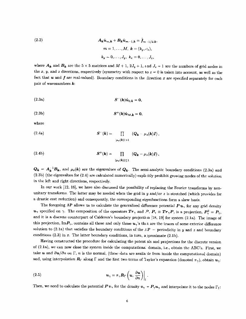
(2.2) AkfZm,k + BkfZm-l,k = J_,_ -1/2,k,

m= 1,...,M, k =_(ky,,:z),

ky=O,...,Jy, kz = 0,...,Jz,

where A k and B k are the 5 × 5 matrices and M + 1, 2J_ + 1, e-nd Jz + 1 are the numbers of grid nodes in

the x, y, and z directions, respectively (symmetry with respect to z -- 0 is taken into account, as well as the

fact that u and j' are real-valued). Boundary conditions in the direction x are specified separately for each

pair of wavenumbers k:

(2.3a) S- (k)f_o,k = O,

(2.3b)

where

(2.4a)

S+(k)'_M,k = o,

s-(k) = II (Qk - ,,(k)Z),

(2.4b) S + (k) -- II (Qk - #_ (k)I),

I_.(k)l_<l

Qk = AklBk, and #s(k) are the eigenvalues of Qk. The semi-analytic boundary conditions (2.3a) and

(2.3b) (the eigenvalues for (2.4) are calculated numerically) explicitly prohibit growing modes of the solution

in the left and right directions, respectively.

In our work [12, 16], we have also discussed the possibility ,5 replacing the Fourier transforms by non-

unitary transforms. The latter may be needed when the grid in y and/or z is stretched (which provides for

a drastic cost reduction) and consequently, the corresponding eigenfunctions form a skew basis.

The foregoing AP allows us to calculate the generalized difference potential P u-r for any grid density

u-r specified on % The composition of the operators Try and D, P-r - Tr-rP, is a projection, P_ -- P'r,

and it is a discrete counterpart of Calderon's boundary projecti, m [18, 19] for system (2.1a). The image of

this projection, ImP-r, contains all those and only those u-r's th;.t are the traces of some exterior difference

solution to (2.1a) that satisfies the boundary conditions of the AP - periodicity in y and z and boundary

conditions (2.3) in x. The latter boundary conditions, in turn, aoproximate (2.1b).

Having constructed the procedure for calculating the potent als and projections for the discrete version

of (2.1a), we can now close thc system inside the computationa: domain, i.e., obtain the ABC's. First, we

take u and Ou/On on F, n is the normal, (these data arc availa fie from inside the computational domain)

and, using interpolation Rr along F and the first two terms of "i aylor's expansion (denoted 7r-r), obtain u-r:

Then, we need to calculate the potential P v-r for the density v-r = P-ru,_ and interpolate it to the nodes F1 :

(2.6) u rl = RrlPv_ =- RrIPuT.

Finally, the ABC's are obtained in the operator form

where Tis composed of the operations of (2.5) and (2.6). Boundary condition (2.7) is applied every time we

need to update the ghost cells when solving the interior problem (e.g., on every iteration). The implemen-

tation of ABC's (2.7) can either be direct or involve preliminary calculation of the matrix T. In the latter

case, the runtime implementation of the ABC's (2.7) is reduced to a matrix-vector multiplication. Numerical

results for flows around the ONERA M6 wing obtained with the DPM°based boundary conditions (2.7) are

summarized in work by Tsynkov and Vatsa [15] and Tsynkov [16, 17].

3. Application to Jet Flows. The major difference between the formulation of the previous section

and the flow with jet exhaust is that in the vicinity of the jet we can no longer claim that flow perturbations

against the free-stream background are small. Indeed, inside the propulsive jet the speed of the flow is

typically much higher than the one in the surrounding area, moreover, other parameters, e.g., temperature,

may also differ substantially. Therefore, the linearization of the flow against constant free-stream background

that yields equations (2.1a), (2.1b) is, generally speaking, not valid in this case.

However, in many applications (in particular, aerospace) one can clearly distinguish between those parts

of the overall flow that contain jet(s) and the remaining areas. Therefore, the most comprehensive way

to develop the far-field linearization in this situation will apparently be to use the appropriate asymptotic

solutions for jets (see, e.g., Abramovich [26]) in the corresponding regions as a background. For flow regions

outside the jet, it is always reasonable to assume that the ]oregoing linearization (2.1) will still be valid there.

The particular setting that we will be studying hereafter is schematically shown in Figure 3.1. (The

meaning of the two external grid surfaces is the same as F and F1 in Figure 2.1.) It includes a three-

dimensional slender body (symmetric with respect to the z = 0 plane but not axially symmetric, i.e., not a

body of revolution) with sharp nose and boat-tail aft configuration; the rearmost plane surface of the body

(not shown explicitly in Figure 3.1) is actually a location of the nozzle outlet; the outlet is rectangular in

cross section. The exterior flow is subsonic with the free-stream Mach number M0 -- 0.6 and zero angle of

attack, the jet that is discharged from the outlet is supersonic, Mj ---- 1.6, and confluent with the exterior

flOW.

The specific shape of the body (see Figure 3.1) as well as parameters of the flow have been previously

proposed for numerical study and analyzed in work by Compton [27]. In this original work [27], Compton had

calculated external flow with the propulsive jet and also considered the interior portion of the flow, namely

the flow in the actual nozzle located inside the afterbody (this nozzle flow obviously produces the jet). For

our study, we have generated new grids and also simplified the overall formulation by eliminating the nozzle

and specifying instead the uniform supersonic flow conditions at the nozzle outlet i.e., at the place where

the jet starts. Compton's goal [27] was to assess the performance of different turbulent models including

their prediction capabilities for the flow inside the nozzle; our goal is to assess the performance of different

external boundary conditions for the flows with jet exhaust. We, therefore, think that the aforcmentioncd

simplification is justified.

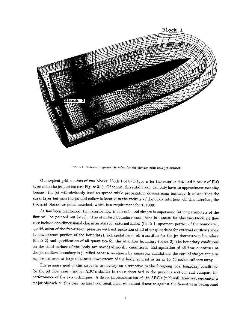
Block 1

FIG. 3.1. Schematic geometric setup for the slender body with jet exhaust.

Our typical grid consists of two blocks: block 1 of C-O type is for the exterior flow and block 2 of H-O

type is for the jet portion (see Figure 3.1). Of coursc, this subdivision can only have an approximate meaning

because the jet will obviously tend to spread while propagating downstream; basically, it means that the

shear layer between the jet and coflow is located in the vicinity of the block interface. On this interface, the

two grid blocks are point-matched, which is a requirement for TLNS3D.

As has been mentioned, the exterior flow is subsonic and the jet is supersonic (other parameters of the

flow win bc pointed out latcr). The standard boundary condi_ ions in TLNS3D for this two-block jet flow

case include one-dimensional charactcristics for external inflow 0 .lock 1, upstream portion of the boundary),

specification of the free-stream pressure with extrapolation of all other quantities for external outflow (block

1, downstream portion of the boundary), extrapolation of all q lantities for the jet downstream boundary

(block 2) and specification of all quantities for the jet inflow boandary (block 2); the boundary conditions

on the solid surface of the body are standard no-slip conditiol_s. Extrapolation of all flow quantities at

the jet outflow boundary is justified because as shown by numei ous simulations the core of the jet remains

supcrsonic cvcn at large distances downstream of the body, at le _st as far as 40 50 nozzle calibcrs away.

The primary goal of this paper is to develop an alternative ;o the foregoing local boundary conditions

for the jet flow case global ABC's similar to those described in the previous section, and compare the

performance of the two techniques. A direct implementation of ;he ABC's (2.7) will, however, encounter a

major obstacle in this case: as has been mentioned, wc cannot li.marize against the frce-strcam background

in thejet regionandtherefore,cannotdirectlyimplementtheoperatorT of (2.7) over the entire external

boundary as this operator is obtained on the basis of the linear system (2.1). Of course, if we linearized

the flow against constant free-stream background outside the jet and against some approximate asymptotic

solution in the jet region (see Ref. [26]) and then used the corresponding linear system (unlike (2.1a), it will

have variable coefficients) to construct the operator analogous to T of (2.7), then we could have applied

the boundary conditions (2.7) straightforwardly as done in the previous work [15, 16] for flows with no

jets. Computation of the new operator T in this framework will, in turn, require a different construction

of the AP, certainly more elaborate (because of variable coefficients) and possibly more expensive than the

one described in the previous section (see formulae (2.3), (2.4), (2.5)). One way of largely eliminating the

difficulties associated with variable coefficients is apparently to take advantage of the supersonic nature of the

jet and use marching-type algorithms in a subdomain of the new AP domain. Although this may make the

whole foregoing program feasible, we consider its implementation as future work. In this paper we present

the algorithm based on boundary conditions (2.7) with minimal alterations.

As the ABC's (2.7) obviously cannot be applied in the jet area, i.e., on that portion of the artificial

boundary where the jet exits the domain, we need another procedure. The most natural choice will be

to extrapolate all flow quantities downstream at the outflow boundary because the core of the jet remains

supersonic even at large distances away from the nozzle outlet. Of course, we cannot actually predict where

on the downstream boundary the flow actually becomes subsonic, i.e., where the extrapolation ceases to be

applicable. However, we have observed that for the particular case under study we can extrapolate at least

on the entire downstream boundary of the second grid block (see Figure 3.1). Thus, extrapolation of all flow

quantities will be used henceforth as downstream boundary conditions ]or block 2.

In the standard procedure, the downstream boundary conditions for grid block 1, i.e., on the rest of

the outflow boundary, are based on the specification of free-stream pressure and extrapolation of all other

quantities. Basically, these boundary conditions are relevant for subsonic outflow. In practice, some portion

of the downstream boundary of block 1 may also be supersonic; in this case, however, the implementation of

these pressure boundary conditions does not lead to noticeable errors because the streamwise variations of

pressure away from the nozzle arc small (the jet is close to design, it is slightly ovcrcxpanded, see below) and

therefore, specification of the free-stream pressure and extrapolation from the interior are both procedures

with acceptable accuracy.

To replace local boundary conditions on the outer boundary of block 1 (the region outside the jet) by the

more accurate global ABC's, we use relation (2.7). However, in formula (2.7) both the input and output are

global, i.e., not only the operator T provides the ghost cell data along the entire boundary but also requires

the data along the entire (penultimate) boundary as driving terms. By using extrapolation downstream in

the jet core instead of using (2.7), we make sure that the possibly erroneous data from the global procedure

are not used on this part of the boundary. However, as the global operator T is constructed on the basis of

linearization (2.1), which is not valid in the jet area, plugging the actual flow quantities (including the jet

profile) into the right-hand side of (2.7) may potentially generate errors along the entire outer boundary.

On the other hand, it has been verified for model examples [14] and also seen for more complex cases

that typically, closely located boundary nodes influence one another much stronger than the remote ones.

This is a reasonable behavior from the standpoint of physics; in the structure of operators W it is reflected so

that although the matrix is dense (non-locality) its near-diagonal terms arc much larger than the off-diagonal

ones (for systems as opposed to scalar equations, it will be a similar block-wise structure). The specific rate

of decay for the off-diagonal terms can probably be obtained only for the most elementary formulations (e.g.,

theLaplaccequationwithperiodicboundaryconditions).Ho_ever,althoughwccannotobtainanalyticalestimatesforthekernelsinvolvedinoperatorsT of (2.7), we can still make use of the actual (block-wise)

off-diagonal decay in the numerical experiments. In practical terms, this implies that although substituting

the jet profile into the right-hand side of (2. 7) violates the smaU perturbations assumption, the associated

error on the left-hand side of (2.7) will mostly be concentrated again in the jet area, where the results are

not used for boundary conditions anyway as they are overridden by extrapolation.

Thus, the actual combined DPM-based ABC's that we employ for computation of the foregoing jet flow

case are the following. For most of the outer boundary (except the near-jet area) we use formula (2.7) while

substituting the actual flow profile in its right-hand side. For the jet core (outflow boundary for grid block

2) we extrapolate all flow quantities downstream. For the small intermediate portion of the downstream

boundary (near the jet core) we extrapolate all quantities except pressure, the latter is prescribed from

its free-stream value. In fact, we have observed that within a certain range (5 to 30 ceils of the fine grid

described in Numerical Results), the actual location of where to switch from the pressure boundary condition

to formula (2.7) does not exert much influence on either the final accuracy or multigrid convergence rate. In

the next subsection, we provide an additional justification for the use of this procedure.

3.1. Jet Outflow Boundary Conditions. To describe and explain the specific boundary treatment

in the vicinity of the jet exit through the boundary, wc start by considering the model problem below,

disregarding for a moment the connection to the global boundary procedure described above.

An model problem describing the error due to inaccurate outflow pressure data for the steady Euler

equations is,

(3.1)Aex + Be_ + Cez = O, a<0,

p=g(y,z), x--O,

-oc < y, z < oo,

where e = (p, u, v,w,p) T denotes the error and A, B, and C are constant matrices. We assume that the

boundary data has compact support outside a small portion of she boundary, i.e.

(3.2) g(y,z) = O, {y,z I >_ ,i,

We also assume that the base flow is subsonic and moves to the 3ight. The problem (3.1),(3.2) is a model for

the error in an approximate solution with correct outflow boundary data given on lY, zl -> 6 and erroneous

one's on lY, zl < 5.

The relation of the model problem (3.1),(3.2) to the specific )utflow problem in this paper can briefly be

described as follows. The global boundary procedure far away fr. )m the jet and the extrapolation procedure,

see Refs. [28, 29], in the supersonic part of the jet lead to very s: nall errors, i.e. Igl _ 0. In an intermediate

domain between the supersonic part of the jet and the part wtle'e the global boundary conditions are used,

pressure with erroneous data is specified, i.e. 191_ O(1) in that part of the domain.

Note that for problems with boundary conditions in the ._" (or streamwise) direction it makes little

difference if one consider the inviscid Euler equations instead of tt e viscous thin layer Navier-Stokes equations

since the number and nature of the boundary conditions require( Lin the x direction are the same for the two

sets of equations.

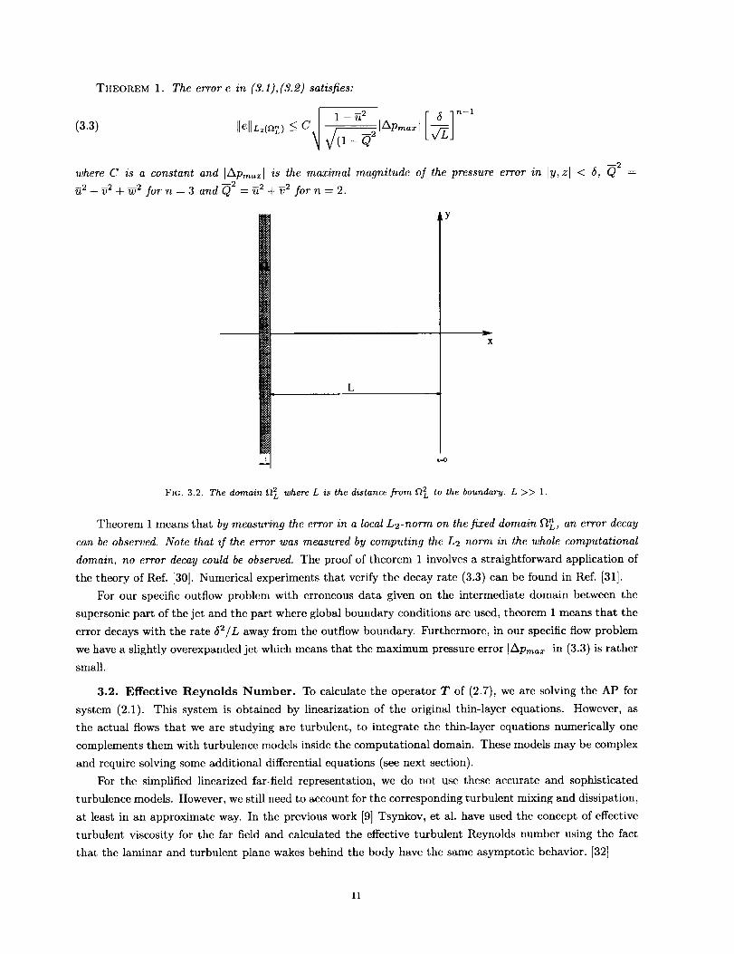
Let _ = ([-(L + 1),-L] x R n-l) where n is the number of spatial dimensions, scc Figure 3.2. The

following theorem describes the error distribution in the halfspa_.'e x < 0.

10

THEOREM 1. The error e in (3.1),(3.2) satisfies:

°-1(3.3) IlellL_(aZ) --<C _lAPm_xf [_j_/(1 -Q-

where C is a constant and IApm_zl is the maximal magnitude of the pressure error in ]y, z I

_2 + 52 + _2 for n = 3 and _2 = _2 + 52 for n = 2.

kY

X

L

< 5,_2

_--o

FIG. 3.2. The domain f12L where L is the distance from 122Lto the boundary. L >> 1.

Theorem 1 means that by measuring the error in a local L2-norm on the fixed domain _, an error decay

can be observed. Note that if the error was measured by computing the L2 norm in the whole computational

domain, no error decay could be observed. The proof of theorem 1 involves a straightforward application of

the theory of Ref. [30]. Numerical experiments that verify the decay rate (3.3) can be found in Rcf. [31].

For our specific outflow problem with erroneous data given on the intermediate domain between the

supersonic part of the jet and the part where global boundary conditions arc used, theorem 1 means that the

error decays with the rate 52/L away from the outflow boundary. Furthermore, in our specific flow problem

we have a slightly overexpanded jet which means that the maximum pressure error IApmax ] in (3.3) is rather

small.

3.2. Effective Reynolds Number. To calculate the operator T of (2.7), we are solving the AP for

system (2.1). This system is obtained by linearization of the original thin-layer equations. However, as

the actual flows that we arc studying are turbulent, to integrate thc thin-layer equations numerically one

complements them with turbulence models inside the computational domain. These models may be complex

and require solving some additional differential equations (see next section).

For the simplified linearized far-field representation, we do not use these accurate and sophisticated

turbulence models. However, we still need to account for the corresponding turbulent mixing and dissipation,

at least in an approximate way. In the previous work [9] Tsynkov, et al. have used the concept of effective

turbulent viscosity for the far field and calculated the effective turbulent Reynolds number using the fact

that the laminar and turbulent plane wakes behind the body have the same asymptotic behavior. [32]

11

The asymptotic behavior of laminar and turbulent circular )ets is also known to bc the same [26, 32]. It

involves a linear increase in width and a decrease in center-line velocity inverse proportional to the distance

from the source. The virtual kinematic viscosity (incompressib e case) can be considered constant through

the entire jet region. Although we do not use boundary conditions (2.7) in the core of the jet, the outer

portions of the shear layer region are still covered by the global procedure, therefore we need to provide the

effective value of 1�Re in equations (2.1).

The jet that we are studying is rectangular in its initial cross section (see next section for particular

details); however, its shape will approach circular further away of the outlet. Therefore, wc will use the

results obtained for circular jets to find an approximate value for the effective Reynolds number. First, we

notice that the universal velocity profiles in a cross section of an incompressible submerged jet (i.e., the

jet that propagates through a medium at rest) are the same _s those obtained for the excess velocity of

the jet propagating in a coflow. [26] Moreover, many experim( ntal observations corroborate [26] that the

same universal profiles remain valid for a compressible supersor:ic jet spreading through either a stationary

or moving medium. Of course, while the profiles are universai, the actual spreading rate for the jet will

differ for different cases. Second, for the particular case under atudy (the ratio of stagnation temperatures

is T_/T_ = 0.936; the design pressure ratio is p_/PO]design = 4.25 at Mj = 1.6 whereas the actual pressure

ratio is P_/Po = 4.00, the jet is slightly overexpanded), the initial value of the compressibility parameter [26]

is p = Po/pj = 1.41 and the initial velocity ratio is m = uo/u_ = _Mo/Mj = 0.459. According to

Rcf. [26], these values are within the range (0 < m < 0.6, 0.3 < p < 1.43), for which the correction due to

compressibility for the spreading rate b of the jet can be taken into account by calculating it as

l+f 1-m(3.4a) bcomp = ax---

2 1 +pro

instead of the old expression

1-m

(3.4b) binc = cx--,l+m

which is relevant for the incompressible flow; c in formulae (3.4) is a constant and x is the distance from the

source.

According to the measurements referenced by Schlichting [32[, for a submerged incompressible jet bl/2 =

0.0848x, where bl/2 is half width of the jet at half depth. Su[stituting this into the solution for laminar

jet [26, 32]:

bl/__22= 5.27 vx v_'

one obtains the virtual kinematic viscosity [32]:

(3.5) /"T = 0.016IVY,

here K is the total kinematic momentum flux. Since the velo :ity profiles are universal, for the jet with

coflow we only need to multiply the spreading rate by (1 - m)/( 1 + m) according to formula (3.4b) and for

the compressibility correction wc use (3.4a), which altogether yi_;lds:

12

(3.6) UT = 0.00636V_.

As has been mentioned, the boundary condition that we specify for the jet inflow is a uniform supersonic

profile across the entire nozzle outlet. Therefore, the quantity K can be obtained by multiplying the square

of the excess velocity (relative velocity of the jet with respect to the velocity of coflow) by the area of the

outlet a, K = (uj - u0)2a. Then, the effective turbulent Reynolds number is calculated as ReT = UL/tJT,

where U is the characteristic speed and L is the characteristic length. For the particular setting under study,

it is reasonable to assume that U = [uj - uo[ and L = v#_. Consequently, from (3.6) we conclude that

(3.7) ReT ----0.00636 -1 _ 157.

In our computations, the actual value of Re for system (2.1) was taken from (3.7).

4. Numerical Results. The particular geometry of the body shown in Figure 3.1 is the following:

rectangular cross section y × z = 6.2 x 6.8 with rounded edges; sharp nose and boat-tail aftcrbody; total

length in the x direction is 63; rectangular nozzle outlet y × z = 2.62 x 5.12; full description can be found in

the work by Compton [27].

The geometry and the flow are symmetric with respect to the plane z = 0 (zero angle of attack). For

our computations we have used three different domains with successively reduced dimensions, see Figure 4.1;

domain I (or large domain) with the diameter of about 30 calibers of the body was used for calculating the

reference solutions, domain II is 0.36 or about 1/3 of the size of domain I in each direction and domain III

is 0.22 or about 1/5 of the size of domain I in each direction.

j/_ Domain I

///

//

\\

\,

/_/ Domain lI (0.36)

//_ DomainIIl (0.22) t

\

\..

FIG. 4.1. Three computational domains .for the jet flow, projection onto the z = 0 plane.

13

Ashasbeenmentioned,to integratethethin-layerequation:,onthecurvilineargridshownonFigure3.1weusethecodeTLNS3DbyVatsa,etal. [23,24]Thisisacentral-differencccodewithfivestageexplicitpseudo-timcRunge-Kuttarelaxationusedforobtainingsteady-statesolutions.ThecodeemployslocalCourantstep,semi-implicitresidualsmoothing,andmultigridforacceleratingtheconvergence.In ourcomputations,weusedeitherthreeor twonestedgridlevelswithV cycles(dependingonthegriddimension);thismulti-levelV-cyclealgorithmis,in fact,a finalstageof thcfull multigrid(FMG)procedure.In addition,to improvetheconvcrgcnceto steadystate,thesolverispreconditionedac_:ordingto themethodologyofRef.[33].

TheDPM-basedABC'sarcimplementedonlyonthefinestgridfortheV-cyclein thefinalFMGstage;theboundarydataforcoarserlcvelsareprovidedbythecoarseningprocedure.Moreover,evenonthisfinestgridweimplementtheDPM-basedABC'sonlyonthefirstandthe last Runge-Kutta stages, which has been

found I15, 16] to make very little difference compared to the implementation on all five stages; the boundary

data for the three intermediate stages are provided from the DPM-based ABC's on the first stage.

To account for the turbulent phenomena, the solver is also supplemented with Menter's two-equation

turbulence model [34]. The actual molecular Reynolds number based on unit length is Re = 321000, Prandtl

number is Pr = 0.72, specific ratio is _ = 1.4.

We have used several different grids to calculate the jet flew; in all cases we kept the normal spacing

near the solid surface thc samc: _ 3.10 -4. All grids are stretched, the cell size increases away of the body in

geometric progression. The dimension of the C-O grid block 1 fo_" domain I was i x j x k = 385 x 77 x 33 (i is

thc streamwise C-type coordinate, j is the radial coordinate, and k is the circumferential cross-stream O-type

coordinate, quarter circle). The dimension of the H-O grid block 2 for domain I was i x j x k = 81 x 77 x 65

(i is streamwise, j is radial, and k covers half circle). We wi_ further refer to this grid as fine. On the

fine grid, we havc calculated two rcference solutions, one with standard ABC's and another with global

ABC's. As the artificial boundary for domain I is locatcd suffi,'iently far away of the body, the difference

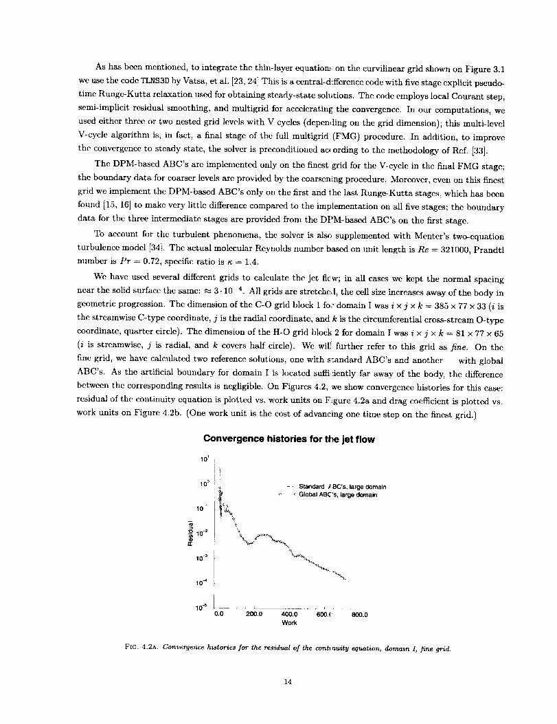
between the corresponding results is negligible. On Figures 4.2, we show convergence histories for this case:

residual of the continuity equation is plotted vs. work units on F-gure 4.2a and drag coefficient is plotted vs.

work units on Figure 4.2b. (One work unit is the cost of advancing one time step on the finest grid.)

10-_

10 2

n,-

I0 -s

10_'

10 -s

Convergence histories for the jet flow

10' i

Iv

10° ! ' Standard /:BC's, largeclomain

i o o Global ABC's, large domain

0.0 200.0 400.0 600.( 800.0

Work

FIe;. 4.2A. Convergence histories for the residual of the contt auity equation, domain I, fine grid.

14

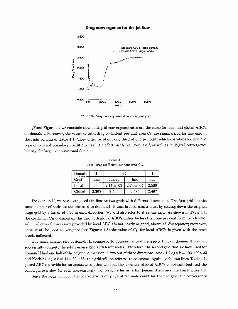
Drag convergence for the jet flow

3,500

O

E3

3.000

2,500

2.000f¢,

0.500 _ •0.0 200.0

Standard ABC's, large domain

_, _ Global ABC's, large domain

J _ L ....... i

400.0 600.0 800.0

Work

FIG. 4.2B. Drag convergence, domain I, fine grad.

LFrom Figure 4.2 we conclude that multigrid convergence rates arc the same for local and global ABC's

on domain I. Moreover, the values of total drag coefficient per unit area Co are summarized for this case in

the right column of Table 4.1. They differ by about one third of one per cent, which corroborates that the

type of external boundary conditions has little effect on the solution itself, as well as multigrid convergence

history, for large computational domains.

TABLE 4.1

Total drag coei_icicnt per unit area CD.

Domain

Grid fine

Local

Global 2.365

III II

coarse fine

2.77 + .03 2.74-t- .04

2.495 2.484

I

fine

2.506

2.497

For domain II, we have computed the flow on two grids with different dimensions• The first grid has the

same number of nodes as the one used in domain I; it was, in fact, constructed by scaling down the original

large grid by a factor of 0.36 in each direction. We will also refer to it as fine grid. As shown in Table 4.1,

the coefficient Co obtained on this grid with global ABC's differs by less than one per cent from its reference

value, whereas the accuracy provided by local ABC's is not nearly as good, about 9% discrepancy; moreover,

because of the poor convergence (see Figures 4.3) the value of CD for local ABC's is given with the error

bands indicated.

The much smaller size of domain II compared to domain I actually suggests that on domain II one can

successfully compute the solution on a grid with fewer nodes. Therefore, the second grid that we have used for

domain II had one half of the original dimension in two out of three directions, block 1 i x j x k = 193 x 39 × 33

and block 2 i x j × k = 41 x 39 x 65, this grid will be referred to as coarse. Again, as follows from Table 4.1,

global ABC's provide for an accurate solution whereas the accuracy of local ABC's is not sufficient and the

convergence is slow (or even non-existent). Convergence histories for domain II are presented on Figures 4.3.

Since the node count for the coarse grid is only 1/4 of the node count for the fine grid, the convergence

15

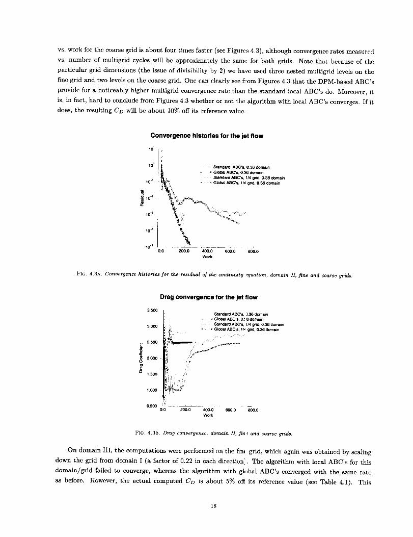
vs. work for the coarse grid is about four times faster (see Figures 4.3), although convergence rates measured

vs. number of multigrid cycles will be approximately the sam,, for both grids. Note that bccause of the

particular grid dimensions (the issue of divisibility by 2) we have used three nested multigrid levels on the

fine grid and two levels on the coarse grid. One can clearly sec _om Figures 4.3 that the DPM-bascd ABC's

provide for a noticeably higher multigrid convergence rate than the standard local ABC's do. Moreover, it

is, in fact, hard to conclude from Figures 4.3 whether or not the algorithm with local ABC's converges. If it

does, the resulting Co will be about 10% off its reference value.

Convergence histories for the jet flow

10 _

10 °

10 -1

10 _

rr

10 -3

104

10 -5

___ Standard ABC's, 0.36 domain

o Global ABC's, 0.36 domain

- - - Standard ABC's, 1/4 grid, 0.36 domain

_ Global ABC's, 1/4 grid, 0.36 domain

, .\0.0 200.0 400.0 600.0 800.0

Work

Fro. 4.3a. Convergence histories for the residual of the continuity equation, domain II, fine and coarse grids.

a

Drag convergence for the jet flow

Standard ABC's, )36 domain

• _ Global ABC's, 0.: 6 domain

Standard ABC's, I/4 grid, 0.36 domain

_ Global ABC's, I/L grid, 0.36 domain

/

_tmmlmmmD /_ -•

iI ,

3.500

3.OOO

2.500 •

2.000

1.500

1.000

0.500 ............ • ....

0.0 200.0 400.0 600.0 800.0

Work

FIG. 4.3B. Drag convergence, domain II, fin _ and coarse grads.

On domain III, the computations were performed on the fin( grid, which again was obtained by scaling

down the grid from domain I (a factor of 0.22 in each direction). The algorithm with local ABC's for this

domain/grid failed to converge, whereas the algorithm with gl,)bal ABC's converged with the same rate

as before. However, the actual computed CD is about 5% off its reference value (see Table 4.1). This

16

canapparentlybeattributedto thefactthattheassumptionof linearity(smallperturbations)outsidethecomputationaldomainis violatedfor sucha smalldomainsize.ConvergencehistoriesfordomainIII areprcscntedonFigures4.4.

Convergence histories for the jet flow

104

10 -s

Standard ABC's, 0.22 domain

o Global ABC's, 0.22 domain

0.0 200.0 400.0 600.0 800.0

Work

F]G. 4.4A. Convergence histories for the residual of the continuity equation, domain III, fine grad.

"5.fi

o0

¢_

Drag convergence for the jet flow

4,000

3.500

3.000 :

2.500

2.000

1.500

1.000

0.500 _0.0

I1'1 /

i' '.. 'lI

IllI Ii,

II II IiI'll I̧ iI

'i II' 'll,

Standard ABC's, 0.22 domain

¢_ _ Global ABC's, 0.22 domain

I A ..... L ....

200.0 400.0 600.0 800.0

Work

FIG. 4.413. Drag convergence, domain IH, fine grid.

Computations on a coarse grid for domain III were not performed because we did not expect to recover

the accurate value of Co. However, the fact that the algorithm with global ABC's converges on domain III

corroborates the high robustness of this procedure.

All computations described in this section were conducted on Cray Research computers, J90 and C90

series. Computational overhead due to the use of global ABC's is about 15% for the particular fine grid

17

referencedbefore.Thisoverheadis determinedmostlybydoIlaingeometryandtypicallydoesnot scalelinearlywith thedimensionofinteriorgrid.Fortheaforementic,nedcoarsegridtheoverheadreaches30_0.

5. Conclusions.WehaveconstructedandimplementedglobalABC'sfor calculatingexternalflowswith jet exhaust.TheABC'scombineextrapolationof all flow quantities downstream in the supersonic

core of the jet and nonlocal DPM-based treatment for the r,;maining portion of outer boundary. The

overhead associated with implementation of the new technique is is compensated for by the reduced grid

dimension on small domains and higher convergence rate. In the series of computations performed, the

DPM-based algorithm have consistently demonstrated better accuracy, faster multigrid convergence, and

higher robustness compared to the standard local methodology.

6. Acknowledgment. We are most grateful to Dr. E. B. Parlettc of Vigyan, Inc., for his valuable help

in grid generation.

REFERENCES

[1] GIVOLI, D., Non-reflecting Boundary Conditions, Journal _,f Computational Physics 94, No. 1 (1991),

pp. 1 29.

[2] GIVOLI, D., Numerical Methods for Problems in Infinite D)mains, Elsevier, Amsterdam, 1992.

[3] TSYNKOV, S. V., Numerical Solution of Problems on Unbounded Domains. A Review, Applied Numer-

ical Mathematics 27, No. 4 (1998), pp. 465 532.

[4] RYABEN'KII, V. S., Boundary Equations with Projections, Russian Mathematical Surveys 40, No. 2

(1985), pp. 147 183.

[5] RYABEN'KII, V. S., Difference Potentials Method for Some Problems of Continuous Media Mechanics,

Nauka, Moscow, 1987 (in Russian).

[6] RYABEN'KII, V. S., Difference; Potentials Method and Its Applications, Math. Nachr. 177 (Feb. 1996),

pp. 251 264.

[7] RYABEN'KII, V. S. AND TSYNKOV, S. V., Artificial Boundary Conditions for the Numerical Solution of

External Viscous Flow Problems, SIAM Journal on Numerical Analysis 32, No. 5 (1995), pp. 1355

1389.

[8] TSYNKOV, S. V., An Application of Nonlocal External (bnditions to Viscous Flow Computations,

Journal of Computational Physics 116, No. 2 (1995), PI'. 212 225.

[9] TSYNKOV, S. V., TURKEL, E., AND ARARBANEL, S., 7_xtcrnal Flow Computations Using Global

Boundary Conditions, AIAA Journal 34, No. 4 (1996), pp. 700-706; also AIAA Paper 95-0564,

(Jan. 1995).

[10] RYABEN'KII, V. S. AND TSYNKOV, S. V., An Effective Nun erical Technique for Solving a Special Class

of Ordinary Difference Equations, Applied Numerical M_thematics 18, No. 4 (1995), pp. 489 501.

[11] TSYNKOV, S. V., Artificial Boundary Conditions for Comp_ ration of Oscillating External Flows, SIAM

Journal on Scientific Computing 18, No. 6 (1997), pp. 1 i12 1656.

[12] RYABEN'KII, V. S. AND TSYNKOV, S. V., An Application o] the Difference Potentials Method to Solving

External Problems in CFD, CFD Review 1998, M. Hafe:; and K. Oshima, eds., (to bc published).

[13] TSYNKOV, S. V., Nonloeal Artificial Boundary Conditions for Computation of External Viscous

Flows, Computational Fluid Dynamics '96. Proceedings ,3f the Third ECCOMAS CFD Conference,

P. Le Tallec and J. P6riaux, eds., John Wiley & Sons, New York, 1996, pp. 512-518.

18

[14] TSYNKOV, S. V., Artificial Boundary Conditions for Infinite-Domain Problems, Barriers and Challenges

in Computational Fluid Dynamics, M. D. Salas et al., eds., Kluwer Academic Publishers, Dordrecht,

The Netherlands, 1998, pp. 119 138.

[15] TSYNKOV, S. V. AND VATSA, V. N., Improved Treatment of External Boundary Conditions for Three-

Dimensional Flow Computations, AIAA Journal 36, No. 11 (1998), pp. 1998 2004; also AIAA Paper

97-2074 (June 1997).

[16] TSYNKOV, S. V., External Boundary Conditions for Three-Dimensional Problems of Computational

Aerodynamics, SIAM Journal on Scientific Computing (to be published).

[17] TSYNKOV, S. V., On the Combined Implementation o] Global Boundary Conditions with Central-

Difference Multigrid Flow Solvers, in Proceedings of IUTAM Symposium on Computational Meth-

ods for Unbounded Domains, July 27 31, 1997, University of Colorado at Boulder, T. L. Geers, ed.,

Kluwcr Academic Publishers (to be published).

[18] CALDERON, A. P., Boundary-Value Problems for Elliptic Equations, in Proceedings of the Soviet-

American Conference on Partial Differential Equations at Novosibirsk, Fizmatgiz, Moscow, 1963,

pp. 303 304.

[19] SEELEY, R. T., Singular Integrals and Boundary Value Problems, American Journal of Mathcmatics

88, No. 4 (1966), pp. 781 809.

[20] SWANSON, R. C. AND TURKEL, E., A Multistage Time-Stepping Scheme for the Navier-Stokes Equa-

tions, AIAA Paper 85-0035 (Jan. 1985).

[21] SWANSON, R. C. AND TURKEL, E., Artificial Dissipation and Central Difference Schemes for the Euler

and Navier-Stokes Equations, AIAA Paper 87-1107 (June 1987).

[22] SWANSON, R. C. AND TURKEL_ E., Multistage Schemes with Multigrid for the Euler and Navier-Stokes

Equations. Volume I: Components and Analysis, NASA TP-3631 (Aug. 1997).

[23] VATSA, V. N. AND WEDAN, B., Development of a Multigrid Code for 3-D Navier-Stoke Equations and

Its Application to a Grid-Refinement Study, Computers and Fluids 18 (1990), pp. 391 403.

[24] VATSA, V. N., SANETRIK, M. D., AND PARLETTE, E. B., Development of a Flexible and Efficient

Multigrid-Based Multiblock Flow Solver, AIAA Paper 93-0677 (Jan. 1993).

[25] THOMAS, J. L. AND SALAS, M. D., Far-Field Boundary Conditions for Transonic Lifting Solutions to

the Euler Equations, AIAA Paper No. 85-0020 (Jan. 1985).

[26] ABRAMOVICH, G. N., The Theory of Turbulent Jets, The MIT Prcss, Cambridgc, Massachusetts, 1963.

[27] COMPTON, W. n._ Comparison of Turbulence Models for Nozzle-Afterbody Flows With Propulsive Jets,

NASA TP-3592 (Sept. 1996).

[28] NORDSTROM, J., Accurate Solutions of the Navier-Stokes Equations Despite Unknown Outflow Bound-

ary Data, Journal of Computational Physics 120, No. 2 (1995), pp. 184 205.

[29] NORDSTROM, J., On Extrapolation Procedures at Artificial Outflow Boundaries for the Time-Dependent

Navier-Stokes Equations, Applied Numerical Mathematics 23, No. 4 (1997), pp. 457 468.

[30] HAGSTROM, T. AND NORDSTROM, J., The Analysis o] Extrapolation Boundary Conditions for the

Linearized Euler Equations, private communication.

[31] LINDBERG N., EFRAIMSSON, G., AND NORDSTROM, J., Numerical Investigation of Extrapolation

Boundary Conditions for the Euler Equations, FFA TN 1998-13, Bromma, Sweden, 1998.

[32] SCHLICHTING, H., Boundary-Layer Theory, Mcgraw-Hill, New York, 1979.

[33] TURKEL, E., VATSA, V. N., AND RADESPIEL, R., Preconditioning Methods for Low-Speed Flows, AIAA

Paper 96-2460 (Junc 1996).

19

[34]MENTER,F. R., Per]ormance of Popular Turbulence Mod,_ls for Attached and Separated Adverse Pres-

sure Gradient Flows, AIAA Paper 91-1784 (June 1991_.

2o

Form ApprovedREPORT DOCUMENTATION PAGEOMB No. 0704-0188

Public reportingburdenfor thiscollectionof information;sestimatedto average1 hourperresponse,includingthe time for reviewinginstructions,searchingexistingdatasources,gatheringand maintainingthe data needed,andcompleting andreviewingthe collectionof information._nd commentsregardingthis burdenestimateor anyother aspectoFthiscollectionof information, includ;ngsuggestionsfor reducingthisburden,to WashingtonHeadquartersSew.ces,Directoratefor InforrnatlonOperationsand Reports,1215JefTersonDavis Highway,Suite1204, Arlington,VA 22202-4302,and to the OfSceof Managementand Budget,PaperworkReductlonProject(0704-0188), Washington,DC 20503.

1. AGENCY USE ONLY(Leave blank) 2. REPORT DATE I 3. REPORT TYPE AND DATES COVERED

November 1998 I Contractor Report

4. TITLE AND SUBTITLE 5. FUNDING NUMBERS

Global Artificial Boundary Conditions for Computation of Extcrna

Flow Problems with Propulsive Jets

6. AUTHOR(S)

Semyon Tsynkov, Saul Abarbanel, Jan Nordstrbm,

Viktor Ryaben'kii, and Veer Vatsa

7. PERFORMING ORGANIZATION NAME(S) AND ADDRESS(ES)

Institute for Computer Applications in Science and Engineering

Mail Stop 403, NASA Langley Research Center

Hampton, VA 23681-2199

9. SPONSORING/MONITORING AGENCY NAME(S) AND ADDRESS(ES)

National Aeronautics and Space Administration

Langley Research Center

Hampton, VA 23681-2199

C NAS1-97046

WU 505-90-52-01

8. PERFORMING ORGANIZATION

REPORT NUMBER

ICASE Report No. 98-52

10. SPONSORING/MONITORINGAGENCY REPORT NUMBER

NASA/CR-1998-208746

ICASE Report No. 98-52

11. SUPPLEMENTARY NOTES

Langley Technical Monitor: Dennis M. Bushnell

Final Report

Submitted to the 14th AIAA CFD Conference, June 1999.

12a. DISTRIBUTION/AVAILABILITY STATEMENT

Unclassified Unlimited

Subject Category 64

Distribution: Nonstandard

Availability: NASA-CASI (301)621-0390

12b. DISTRIBUTION CODE

13. ABSTRACT (Maximum 200 words)

Wc propose new global artificial boundary conditions (ABC's) f )r computation of flows with propulsive jets.

The algorithm is based on application of the difference potentials method (DPM). Previously, similar boundary

conditions have been implemented for calculation of external comp essible viscous flows around finite bodies. The

proposed modification substantially extends the applicability range of the DPM-based algorithm. In the paper, we

present the general formulation of the problem, describe our numerical methodology, and discuss the corresponding

computational results. The particular configuration that we analyze is a slender three-dimensional body with boat-

tail geometry and supersonic jet exhaust in a subsonic external flow under zero angle of attack. Similarly to the

results obtained earlier for the flows around airfoils and wings, curt mt results for the jet flow case corroborate the

superiority of the DPM-bascd ABC's over standard local methodologies from the standpoints of accuracy, overall

numerical performance, and robustness.

14. SUBJECT TERMS

external flow problems; jet exhaust; artificial boundary conditions;

difference partials method

17. SECURITY CLASSIFICATIONOF REPORT

Unclassified

_SN 7540-01-280-5500

18. SECURITY CLASSIFICATION

OF THIS PAGE

Unclassified

15. NUMBER OF PAGES

25

16. PRICE CODE

A0319. SECURITY CLASSIFICATION 20. LIMITATION

OF ABSTRACT OF ABSTRACT

i

Standard Fown 298(Rev. 2-89)Prescribed by ANSI Std. Z39-18298-102