Bayesian Structural Equation Models for Cumulative Theory Buildin

8/12/2019 Bayesian Structural Equation Models for Cumulative Theory Buildin

http://slidepdf.com/reader/full/bayesian-structural-equation-models-for-cumulative-theory-buildin 1/13

Association for Information Systems

AIS Electronic Library (AISeL)

AMCIS 2012 Proceedings Proceedings

Bayesian Structural Equation Models forCumulative eory Building in InformationSystems

Joerg Evermann Memorial University of Newfoundland, St. John's, NF, Canada. , [email protected]

Mary TateSchool of Information Management, Victoria University of Wellington, Wellington, New Zealand. , [email protected]

Follow this and additional works at: hp://aisel.aisnet.org/amcis2012

is material is brought to you by the Americas Conference on Information Systems (AMCIS) at AIS Electronic Library (AISeL). It has been accepted

for inclusion in AMCIS 2012 Proceedings by an authorized administrator of AIS Electronic Library (AISeL). For more information, please contact

[email protected].

Recommended Citation Joerg Evermann and Mary Tate, "Bayesian Structural Equation Models for Cumulative eory Building in Information Systems" (July 29, 2012). AMCIS 2012 Proceedings. Paper 1.hp://aisel.aisnet.org/amcis2012/proceedings/ResearchMethods/1

http://aisel.aisnet.org/?utm_source=aisel.aisnet.org%2Famcis2012%2Fproceedings%2FResearchMethods%2F1&utm_medium=PDF&utm_campaign=PDFCoverPages

http://aisel.aisnet.org/amcis2012?utm_source=aisel.aisnet.org%2Famcis2012%2Fproceedings%2FResearchMethods%2F1&utm_medium=PDF&utm_campaign=PDFCoverPages

http://aisel.aisnet.org/amcis2012/proceedings?utm_source=aisel.aisnet.org%2Famcis2012%2Fproceedings%2FResearchMethods%2F1&utm_medium=PDF&utm_campaign=PDFCoverPages


mailto:[email protected]%3E

mailto:[email protected]%3E


http://aisel.aisnet.org/amcis2012/proceedings?utm_source=aisel.aisnet.org%2Famcis2012%2Fproceedings%2FResearchMethods%2F1&utm_medium=PDF&utm_campaign=PDFCoverPages


http://aisel.aisnet.org/?utm_source=aisel.aisnet.org%2Famcis2012%2Fproceedings%2FResearchMethods%2F1&utm_medium=PDF&utm_campaign=PDFCoverPages



Evermann and Tate Bayesian Structural Equation Models

Proceedings of the Eighteenth Americas Conference on Information Systems, Seattle, Washington, August 9-12, 2012. 1

Bayesian Structural Equation Models for Cumulative

Theory Building in Information Systems

Joerg EvermannMemorial University of Newfoundland

[email protected]

Mary TateVictoria University of Wellington

[email protected]

ABSTRACT

Theories are sets of causal relationships between constructs and their proxy indicator variables. Theories are tested and their

numerical parameters are estimated using statistical models of latent and observed variables. A considerable amount of

theoretical development in Information Systems occurs by theory extension or adaptation. Moreover, researchers are

encouraged to reuse existing measurement instruments when possible. As a consequence, there are many cases when a

relationship between two variables (latent and/or observed) is re-estimated in a new study with a new sample or in a new

context. To aid in cumulative theory building, a re-estimation of parameters should take into account our prior knowledge

about their likely values. In this paper, we show how Bayesian statistical models can provide a statistically sound way of

incorporating prior knowledge into parameter estimation, allowing researchers to keep a “running tally” of the best estimates

of model parameters.

Keywords

Quantitative Analysis, Structural Equation Models, Bayesian Statistics

INTRODUCTION

Theories are statements of causal relationships between constructs (Whetten, 1989; Gregor, 2006). Constructs are imbued

with meaning in part by their relationship with other constructs and their relationship with observations. In other words,

besides the relationships specified in the “structural” model between one construct and another, the relationships in the

“measurement” model (those between constructs and observations) are also theoretically interesting and important

constituents of the meaning of the construct (Hayduk, Cummings, Boadu, Pazderka-Robinson, & Boulianne, 2007; Hayduk

& Glaser, 2000).

Constructs are typically represented in statistical models as latent variables (SEM), composites (PLS), components (PCA) or

common factors (EFA). These variables are related to each other and to observed variables, which represent a construct's

indicators, by linear or non-linear relationships. The relationships are parameterized and the parameter values can be

estimated using a range of statistical techniques. These estimated parameter values are part of the theory.

In other words, a construct’s relationship to other variables is not simply characterized by the presence or absence of such a

relationship. It is insufficient to say that A influences B; we need to put a number on the strength of the relationship. For

example, we would like to say not only that IT spending affects competitive advantage, but we need to specify how much

advantage each dollar of IT spending brings. This is common practice in other areas of science. For example, the physical law

relating the temperature (T), pressure (P), and volume (V) of a gas is described as PV=NkT where both N and k are very

precisely measured parameters. Clearly, a theory that yields PV=2NkT is an entirely different theory, although in both

theories temperature, pressure and volume are related in the same manner. In summary, theories that, while structurally

isomorphic, differ in their numerical parameters, are different theories.

Parameter values are important not only for relationships between constructs, but also for relationships between constructsand indicator variables. To use a well known IS example, the meaning of the perceived ease of use construct is not the same

when it is correlated with the indicator “I believe the system is easy to use” at r=0. 6 than when it is correlated at r=0.9

(assuming all else being equal and that the difference is statistically significant beyond random sampling fluctuations). Kim,

Shin, and Grover (2011) coined the term “measurement instability” for this phenomenon. When different models are fitted to

the same data, such changes in measurement properties, which lead to differences in the meaning of constructs, are referred to

as interpretational confounding. When the same model is fitted to different data, e.g. for multiple groups or in longitudinal

studies, the absence of changes in measurement properties is referred to as measurement invariance. Both are special cases of





And further that

(

This yields the following multivariate-normal likelihood function, where and are vectors of the and respectively.

( | (

( ( )

We now need to assume a distribution for the prior probability of the parameters, (, preferably one that makes the

posterior probability easy to compute. The conjugate prior of the multivariate normal distribution is the normal-inverse

gamma distribution. Assuming that the prior mean and variance are independent, we can write

( ( ( |

Where

( (

( | ( ̅

Here, the prior distribution for the variance is an inverse gamma distribution, while the prior distribution for the means,

conditional on prior variance, is a Normal distribution. The latter is assumed to be independent of the prior variance, thus in

effect making it an unconditional distribution and making the priors for means and variances independent.

With these assumptions, the posterior probability distribution can be calculated analytically. The parameters of the prior

distribution ̅ are called hyper-parameters. The parameters and represent our prior knowledge of the means and

variances for the variances of the regression errors . The means and variances of an inverse gamma distribution are

and

(( respectively. Thus, setting and yields a mean of 2 and a variance of

as our prior estimate of the

variances. In other words, the mean of the prior distribution represents our “point estimate” of the parameter value and the

variance represents our uncertainty in this estimate. Similarly, the hyperparameter ̅ represents the mean of the prior

probability and is thus our prior estimate of the parameter . The hyperparameter represents the variance of the prior

probability distribution and thus represents our uncertainty of the estimate .̅ Because the variances represent uncertainty,

texts on Bayesian statistics often re-parameterize the prior probabilities using the inverse variance, called precision. When

there is little prior knowledge, i.e. little certainty about any prior values, an uninformative prior distribution, such as a

uniform distribution may be used. Alternatively, a prior distribution with very small precision, i.e. very large variance, may

be used.

Having developed our statistical model and found a solution for the posterior probability, we are now in a position to estimate

the parameter values from this posterior distribution. This occurs by sampling values of individual parameters from the

posterior distribution one parameter at a time, a process referred to as Gibbs sampling. Using our example, we have

analytically determined the posterior probability distribution to be multivariate normal (because of the multivariate normal

likelihood and the conjugate prior distribution). It is now straightforward to iteratively sample values from this multivariate

normal distribution, e.g. first for from

( | ̅ (Step 1)

and then for from

( | ̅ (Step 2)

Every iteration comprises these two steps. In the first iteration, a starting values for is randomly assumed for step 1. Thisallows sampling of a value for which is then input to step 2 in that same iteration and allows sampling of a value for .

These sampled values form the input for the next iteration of these two steps. The iterations continue until the sampled values

are stable. In practice, it is common to begin multiple of these Markov Chains from different starting values to ensure valid

convergence. Final parameter estimates are then computed as the mean of the sampled values after a “burn-in” period where

stabilization occurs and whose samples are discarded. Typically, there may be up to 10,000 iterations in each of three Markov

Chains, with burn-in periods of between 2,000 and 5,000. These numbers indicate the substantial computational requirements

for Bayesian statistics, especially for complex structural equation models with dozens or hundreds of parameters.





While Bayesian statistics have been known for a long time, their application to structural equation models has been more

recent (Lee, 2007). Moreover, the necessary computing power only now makes their estimation feasible on personal

computers. Finally, easy to use software for Bayesian SEM has only recently been developed, in the form of MCMC

packages for the R system, the BUGS and OpenBUGS software, and inclusion of Bayesian analysis in popular SEM software

packages like Mplus and Amos. In this paper, we illustrate Bayesian SEM using BUGS and OpenBUGS. BUGS (“Bayesian

Inference Using Gibbs Sampling”) is a flexible software package for estimation of Bayesian models, originally developed by

the biostatistics unit at Cambridge University. OpenBUGS is an open-source version of the commercial WinBUGS

implementation, and model definitions are fully interchangeable between the two. We focus on BUGS because of its

flexibility and the fact that model specifications are written in a very explicit form and are therefore easy to understand.

EXAMPLE: BAYESIAN ESTIMATION FOR TAM CONSTRUCTS

We use TAM as an illustrative example because its constructs have been measured consistently using the same measurement

items across multiple studies. Thus, it provides a rich set of prior knowledge about parameter estimates for us to use. TAM

focuses on the relationship among three constructs, Perceived Ease of Use (PEoU), Perceived Usefulness (PU) and

Behavioral Intention to use (BI).

To identify previous estimates for the TAM model parameters, we focus on studies published in five IS journals, MISQ,

JMIS, ISR, JAIS, and ISJ. Through the ISI web of science we identified papers in these journals that cite either Davis (1989)

or Davis et al. (1989), revealing 263 papers. Of these, 43 are empirical papers that use at least some of the TAM indicators

developed by Davis (1989) and Davis et al. (1989). Figure 1 shows box-and-whisker plots of reported standardized loadings

by items. That data is presented in Table 1 (all surveyed studies use 7-point scales). As many of the 43 studies do not use BIas outcome variable, we have compiled prior values only for the loadings of the PEoU and PU constructs.

Figure 1: Standardized Loadings for TAM measurement item





Table 1: Standardized Loadings by TAM measurement item

Item Minimum Median Mean Maximum Variance SEM

PEoU1 .6370 .8600 .8432 .9700 .00586 .0095

PEoU2 .5320 .8550 .8202 .9700 .01261 .0154

PEoU3 .5610 .8600 .8327 .9600 .01028 .0135

PEoU4 .4967 .8800 .8217 .9400 .01526 .0211

PEoU5 .5000 .8800 .8344 .9517 .01260 .0158

PEoU6 .5300 .8800 .8682 .9700 .00562 .0092

PU1 .4100 .8250 .8199 .9300 .00743 .0127

PU2 .7800 .8550 .8652 .9800 .00298 .0105

PU3 .7300 .8800 .8724 .9800 .00421 .0087

PU4 .6200 .8940 .8728 .9673 .00451 .0124

PU5 .6200 .8450 .8309 .9500 .00711 .0124

PU6 .6400 .8600 .8429 .9800 .00622 .0100

A researcher using using TAM constructs such as PU and PEoU in a new study, and choosing to adapt the instrument

pioneered by Davis (1989) and Davis et al. (1989), might be faced with the situation that, despite taking all reasonable

precautions, her data does in fact show statistically significant differences to previously established values. When the

researcher is certain that her instrument does in fact measure the same construct (e.g. changes to the instrument have been

ruled out, sample characteristics are comparable, and the same statistical methods are used), we recommend that researchers

employ Bayesian statistics to reconcile the differences by using the existing, prior knowledge about the parameter values as

inputs to the Bayesian estimation.

To show how this can be done, we have used the TAM data from Chin et al. (2008). First we fitted a CFA model using

traditional Maximum-Likelihood estimation. Then we employed Bayesian estimation of the CFA model to make use of the

prior information in Table 1. The means of the loadings in Table 1 are used as the means of normal prior probability

distributions for the loadings. We ran the Bayesian estimation with three different variances of the normal prior probability

distributions for the loadings to show how researchers can encode different degrees of certainty about the prior model parameter values. The initial estimation used the standard error (s.e.) of the mean of the published estimates from Table 1.

This expresses relatively little certainty about the prior values. The second estimation used 1/10 times the s.e. of the

published estimates, expressing greater certainty about the published estimates, while the third estimation used 1/100 times

the s.e. of the published estimates, expressing even more certainty about the published estimates. Table 2 compares the

parameter estimates of the ML estimation and the Bayesian estimations.

Table 2 shows that the Bayesian estimates and standard errors are of the same order of magnitude as the traditional ML

estimates (column “Bayesian 1” in Table 2, variance of prior probability distribution on factor loadings equals the standard

error of the mean from Table 1). In the Baysian context, the ML estimates can be viewed as posterior estimates with an

uninformative prior distribution because they make no use of existing information about parameter distributions, only of the

sample data. When the certainty of the prior information is increased (column “Bayesian 2” in Table 2, variance of prior

probability distribution on factor loadings equals 1/10 the standard error of the mean from Table 1) estimates for all

parameters tend to be closer to the prior estimates, showing the influence of prior information on the estimates. When the

certainty of the prior estimates is further increased (column “Bayesian 3” in Table 2, variance of prior probability distribution

on factor loadings equals 1/100 the standard error of the mean from Table 1), the estimates tend to be still closer to the prior

estimates. Table 2 also shows that the standard errors for the estimate are smaller when the prior means are more certain, and

larger when the prior means are less certain.





Table 2: CFA model loadings for the Chin et al. (2008) data for different estimation methods

Param. ML Estimate Prior Estimates

(From Table 1)

Bayesian 1 Bayesian 2

(greater certainty)

Bayesian 3

(much greater

certainty)

Estimate Std. Err. Estimate Std. Err. Estimate

(Mean)

Std. Dev. Estimate

(Mean)

Std. Dev. Estimate

(Mean)

Std. Dev.

Eou1 .881 .0468 .8432 .0095 .9078 .0551 .8717 .0234 .8488 .0094

Eou2 .899 .0462 .8202 .0154 .8506 .0531 .8319 .0243 .8242 .0111

Eou3 .922 .0453 .8327 .0135 .8396 .0509 .8270 .0227 .8318 .0104

Eou4 .827 .0486 .8217 .0211 .7128 .0485 .7306 .0266 .7965 .0131

Eou5 .895 .0463 .8344 .0158 .8445 .0529 .8312 .0247 .8341 .0113

Eou6 .939 .0446 .8682 .0092 .9000 .0530 .8802 .0212 .8721 .0088

Use1 .828 .0390 .8199 .0127 .7424 .0453 .7691 .0256 .8106 .0108

Use2 .837 .0406 .8652 .0105 .7983 .0468 .8245 .0248 .8585 .0099

Use3 .845 .0498 .8724 .0087 .8760 .0496 .8708 .0239 .8727 .0091

Use4 .861 .0466 .8728 .0124 .8692 .0491 .8661 .0256 .8724 .0105

Use5 .809 .0595 .8309 .0124 .9092 .0550 .8633 .0281 .8363 .0108

Use6 .880 .0594 .8429 .0100 .9688 .0524 .9016 .0249 .8527 .0097

Phi1,2 .612 .0403 NA NA .6090 .0782 .6106 .0682 .6113 .0683





Using Bayesian estimation methods, it is thus possible to build cumulative evidence of model parameter estimates and to

incorporate prior knowledge in a statistically sound way. This allows researchers to keep a “running tally” of the best

estimates of model parameters.

BAYESIAN DIAGNOSTICS

As any numerical, iterative algorithm, Bayesian estimation can suffer from non-convergence of results. Before interpreting

the results of Bayesian estimation, it is therefore important to perform diagnostic evaluations. To assess convergence of the

Gibbs sampler, it is common practice to have multiple independent sampling “chains”, each with different start values. Two

possible problems can arise and need to be assessed. First, the different Gibbs sampling chains should converge with one

another. Second, each individual chain should be stable. The WinBUGS software, or the coda package in the R software,

can produce diagnostic plots and other diagnostic statistics to assess these potential issues. In our example, we ran three

Gibbs sampling chains using 5000 samples each.

Figure 2 below shows a properly converged solution for one parameter of the model. The trace plot on the left of the figure

shows the sampled values for each of the three chains for the 5000 samples, while the density plot on the right shows the

overall frequency of sampled values for the three chains. We can see that all three sampling chains converge on the same

values and each of the three sampling chains have a stable average. The density plot in Figure 2 confirms this by showing an

approximately normal distribution.

Figure 2: Trace plot and density plot for one parameter of the Bayesian CFA model showing a good solution

Figure 3 below shows a trace plot and a density plot for one parameter of the CFA model that shows convergence problems

of the type that one of the chains produces stable values that differ from those of the other chains. We can see that one of the

chains converged on a different value, which is also reflected in the bimodal density plot on the right of Figure 3. In this

situation, the analysis should be re-run with different starting values for this parameter.

The second issue is the convergence of each individual chain around a stable mean. Figure 4 below shows a trace plot and

density plot for a situation where the individual chains did not converge. We can clearly see that the sampled values fluctuate

wildly around their sliding-window average (solid lines in the trace plot). In this example, the problem resulted fromspecifying too little precision together with an under-identified structural equation model. As the model definition in

Appendix A shows, loadings, errors, and latent variances are all free parameters, leading to an under-identified model. While

in ML-based SEM, model identification can be achieved either by constraining loadings or by constraining the latent

variances, this choice is not provided in BUGS. The BUGS variance/covariance matrix for the prior probabilities of the latent

variables can either be entirely stochastic or entirely deterministic, but not a mixture of both. In other words, we would have

to specify not only the variances, but also the covariance, which is not common practice and for which little theoretical

justification exists in the TAM literature. Alternatively, we would have to constrain a factor loading. However, in our

example, we wished to compare loadings and standard errors for all indicators.





In Bayesian SEM, the sampling of even an under-identified model will converge, when the estimates are stron gly “guided”

by a large precision for the prior probabilities, However, when little precision is specified and the model is under-identified,

the estimation cannot converge, just like in traditional ML-based SEM. We emphasize that the same model identification

criteria apply in Bayesian SEM as they do in covariance analysis.

Figure 3: Trace plot and density plot for one parameter of the Bayesian CFA model showing non-convergence

Figure 4: Trace plot and density plot for one parameter of the Bayesian CFA model showing non-convergence of the

individual sampling chains.

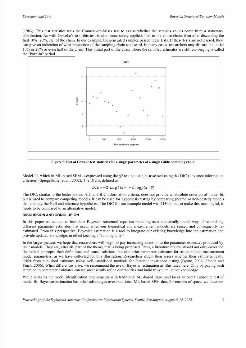
More formally, a number of statistics can be computed to help identify convergence problems. For example, Geweke (1992)

suggested testing the equality of means of the first 10% and the last 50% of the values in the sampling chain to assess the

stability of the estimates. The test statistic is normally distributed and can be used for a z-test. Figure 5 shows an excerpt of

these test statistics, and the 95% confidence interval, for the different parameter estimates. For this plot, the first half of the

Markov chain is divided into 20 segments, then Geweke’s z-score is repeatedly calculated. The first z-score is calculated with

all iterations in the chain, the second after discarding the first segment, the third after discarding the first two segments, and

so on. The last z-score is calculated using only the samples in the second half of the chain. This diagnostic tool can show

which part of the chain is different from the final part. Another test statistic has been proposed by Heidelberger and Welch





(1983). This test statistics uses the Cramer-von-Mises test to assess whether the samples values come from a stationary

distribution. As with Geweke’s test, this test is also successively applied, first to the entire chain, then after discarding the

first 10%, 20%, etc. of the chain. In our example, the generated samples passed these tests. If these tests are not passed, they

can give an indication of what proportion of the sampling chain to discard. In many cases, researchers may discard the initial

10% or 20% or even half of the chain. This initial part of the chain where the sampled estimates are still converging is called

the “burn-in” period.

Figure 5: Plot of Geweke test statistics for a single parameter of a single Gibbs sampling chain

Model fit, which in ML- based SEM is expressed using the χ2 test statistic, is assessed using the DIC (deviance information

criterion) (Spiegelhalter et al., 2002). The DIC is defined as

( |

The DIC, similar to the better known AIC and BIC information criteria, does not provide an absolute criterion of model fit,

but is used to compare competing models. It can be used for hypothesis testing by comparing (nested or non-nested) models

that embody the Null and alternate hypotheses. The DIC for our example model was 7130.0, but to make this meaningful, it

needs to be compared to an alternative model.

DISCUSSION AND CONCLUSION

In this paper we set out to introduce Bayesian structural equation modeling as a statistically sound way of reconciling

different parameter estimates that occur when our theoretical and measurement models are reused and consequently re-

estimated. From this perspective, Bayesian estimation is a tool to integrate our existing knowledge into the estimation and

provide updated knowledge, in effect keeping a “running tally”.

In the larger picture, we hope that researchers will begin to pay increasing attention to the parameter estimates produced bytheir models. They are, after all, part of the theory that is being proposed. Thus, a literature review should not only cover the

theoretical concepts, their definitions and causal relations, but also prior parameter estimates for structural and measurement

model parameters, as we have collected for this illustration. Researchers might then assess whether their estimates really

differ from published estimates using well-established methods for factorial invariance testing (Byrne, 2004; French and

Finch, 2006). When differences arise, we recommend the use of Bayesian estimation as illustrated here. Only by paying such

attention to parameter estimates can we successfully refine our theories and build truly cumulative knowledge.

While it shares the model identification requirements with traditional ML-based SEM, and lacks an overall absolute test of

model fit, Bayesian estimation has other advantages over traditional ML-based SEM that, for reasons of space, we have not





illustrated here (Lee, 2007). For example, by treating missing values in the same way as factor scores or parameter values and

estimating them in the same way as part of the overall model estimation, Bayesian statistics provides an integrated way of

dealing with them, superior to listwise or pairwise deletion. Further, Bayesian SEM has been extended to allow it to include

dichotomous and categorical variables (Lee et al., 2010), nonlinear models (Lee et al., 2007), multi-level models (Song and

Lee, 2008) and finite mixtures within SEM (Lee, 2007), all of which are problematic in traditional ML based SEM.

From a pragmatic perspective, Bayesian SEM are easy to apply, as the model definition in Appendix A shows. It is easy to

see, for example, how such a model might be extended to deal with multi-level, i.e. nested, data and different level-1 andlevel-2 predictors. The explicit specification of the model makes it easy to understand and easy to diagnose. Combined with

the wide availability in commercial software such as AMOS or MPlus and open source software such as OpenBUGS and R,

and with increasingly powerful personal computers, Bayesian estimation is rapidly becoming an easy-to-use tool.

REFERENCES

Byrne, B. M. 2004. “Testing for multigroup invariance using AMOS graphics: A road less traveled,” Structural Equation

Modeling , (11:2), pp. 272 – 300.

Chin, W. W., Johnson, N., and Schwarz, A. 2008. “A fast form approach to measuring technology acceptance and other

constructs,” MIS Quarterly, (32:4), pp. 687 – 703.

Congdon, P. 2006. Bayesian Statistical Modelling 2nd ed. Chichester, England: John Wiley & Sons, Ltd.

Davis, F. 1989. “Perceived usefulness, perceived ease of use, and user acceptance of information technology,” MIS

Quarterly, (13), pp. 319 – 340.

Davis, F., Bagozzi, R., and Warshaw, P. 1989. “User acceptance of computer technology: A com parison of two theoretical

models,” Management Science, (35), pp. 982 – 1002.

French, B. F. and Finch, W. H. 2006. “Confirmatory factor analytic procedures for the determination of measurement

invariance,” Structural Equation Modeling , (13:3), pp. 378 – 402.

Gelman, A., Carlin, J.B., Stern, H.S. and Rubin, D.B. 2003. Bayesian Data Analysis, 2nd ed. London: CRC Press.

Geweke, J. 1992. “Evaluating the accuracy of sampling-based approaches to calculating posterior moments. In Bayesian

Statistics 4 (ed. J.M. Bernado, J.O. Berger, A.P. Dawid and A.F.M. Smith). Clarendon Press, Oxford, UK.

Gregor, S. 2006. “The nature of theory in information systems,” MIS Quarterly, (30:3), pp. 611 – 642.

Heidelberger, P. and Welch, P.D. 1983. “Simulation run length control in the presence of an initial transient.” Operations

Research 31, 1109-1144.

Hayduk, L. A. and Glaser, D. N. 2000. “Jiving the four step, waltzing around factor analysis, and other serious fun,”

Structural Equation Modeling , (7:1), pp. 1 – 35.

Hayduk, L., Cummings, G., Boadu, K., Pazderka-Robinson, H., & Boulianne, S. (2007). “Testing! testing! one, two, three – Testing the theory in structural equation models!” Personality and Individual Differences, 42(5), 841-850.

Kim, G., Shin, B. and Grover, V. 2010. “Investigating Two Contradictory Views of Formative Measurement in Information

Systems Research,” MIS Quarterly, (34:2), pp. 345-365.

Lee, S.Y. 2007. Structural Equation Modeling – A Bayesian Approach. John Wiley & Sons, Chichester, England.

Lee, S.Y., Song, X.Y. and Tang, N.S. 2007. “Bayesian methods for analyzing structural equation models with covariates,

interaction, and quadratic latent variables,” Structural Equation Modeling, (14:3), 404-434.

Lee, S.Y., Song, X.Y. and Cai, J.H. 2010. “A Bayesian approach for nonlinear structural equation models with dichotomous

variables using Logit and Probit links,” Structural Equation Modeling, (17:2), 280-302.

Song, X.Y. and Lee, S.Y. 2008. “A Bayesian approach for analyzing hierarchical data with mi ssing outcomes through

structural equation models,” Structural Equation Modeling, (15:2), 272-300.

Speigelhalter, D.J., Best, N.G., Carlin, BP. And van der Linde, A. 2002. “Bayesian measure of model complexity and fit,”

Journal of the Royal Statistical Society, Series B (64:4), 583-639.Whetten, D. A. 1989. “What constitutes a theoretical contribution?” The Academy of Management Review, (14:4), pp. 490–

495.





APPENDIX A: BUGS MODELS FOR USE WITH WINBUGS OR OPENBUGS

The following table shows a commented BUGS model that was used for the analyses in this paper. One noteworthy feature is

the use of inverse variances (i.e. precisions) in BUGS models, as is common in the Bayesian literature. Thus, larger values

indicate higher degrees of certainty. This model definition works with both the WinBUGS and the OpenBUGS software. For

this study, we used OpenBUGS version 3.2.1 rev 781 on a Linux operating system.

1 model {2 for(i in 1:N){ The model is set up for each of the N observations

3 #measurement equation model

4 for(j in 1:P){ Specify a normal distribution of the observed values y

5 y[i,j]~dnorm(mu[i,j],psi[j]) with means mu and inverse covariance (precision) psi

6 ephat[i,j]<-y[i,j]-mu[i,j] The error ephat is observed y minus explained part mu

7 }

8 mu[i,1]<-lam[1]*xi[i,1] The explained part of each variable as a product

9 mu[i,2]<-lam[2]*xi[i,1] of loading lam and factor score xi[i, 1]

10 mu[i,3]<-lam[3]*xi[i,1]

11 mu[i,4]<-lam[4]*xi[i,1]

12 mu[i,5]<-lam[5]*xi[i,1]

13 mu[i,6]<-lam[6]*xi[i,1]

14 mu[i,7]<-lam[7]*xi[i,2] The second seven items load on the other factor with

15 mu[i,8]<-lam[8]*xi[i,2] Factor scores xi[i, 2]

16 mu[i,9]<-lam[9]*xi[i,2]

17 mu[i,10]<-lam[10]*xi[i,2]

18 mu[i,11]<-lam[11]*xi[i,2]

19 mu[i,12]<-lam[12]*xi[i,2]

20 #structural equation model

21 xi[i,1:2]~dmnorm(u[1:2],phi[1:2,1:2]) The factors are multivariate normally distributed with

22 } #end of i means u and inverse covariance (precision) phi.

23 #priors on loadings

24 lam[1]~dnorm(0.8432,105) Specify a normal distribution of the loadings with means

25 lam[2]~dnorm(0.8202,64) and inverse variances (precision) taken from prior

26 lam[3]~dnorm(0.8327,74) literature

27 lam[4]~dnorm(0.8217,47)

28 lam[5]~dnorm(0.8344,63)

29 lam[6]~dnorm(0.8682,108)

30 lam[7]~dnorm(0.8199,78)

31 lam[8]~dnorm(0.8652,95)

32 lam[9]~dnorm(0.8724,114)

33 lam[10]~dnorm(0.8728,80)

34 lam[11]~dnorm(0.8309,80)

35 lam[12]~dnorm(0.8429,100)

36 #priors on errors

37 for(j in 1:P){

38 psi[j]~dgamma(9.0, 4.0) Specify a gamma distribution for the error variances (the

39 } random part of y)

40 #priors on latent (co-)variances

41 phi[1:2,1:2] ~ dwish(R[1:2,1:2], 5) Specify a Wishart distribution for the covariances of the42 } #end of model factors





While we did not have sufficient data on the TAM outcome variables and estimates for the structural coefficients of the TAM

model, the above BUGS model is easily extended to a full SEM model. For example, an endogenous latent variable could be

introduced by adding the following definitions.

21a eta[i]~dnorm(nu[i],psd)Latent variable eta is defined as normally distributed with mean

nu and precision psd.

21b nu[i]<-gam[1]*xi[i,1]+gam[2]*xi[i,2]

This is the core structural model: the mean nu of eta (i.e. the

explained part) is defined as the weighted product of the twoexogenous latent variables xi

21c dthat[i]<-eta[i]-nu[i]The random part (disturbance) of eta is eta minus the

explained part nu.

35a for(j in 1:2){gam[j]~dnorm(0.5, psd)}Specify normal distributions on the gam structural coefficients

with a given mean and precision psd

35b psd~dgamma(9.0, 4.0)Specify a gamma distribution with given hyper-parameters forpsd

Means models can be added easily by adding variable means and their prior probability distributions, as in the following

example, which also introduces model identification by scaling one of the indicator loadings.

8 mu[i,1]<-xi[i, 1]+alp[1]

Add an intercept alp to the explained part mu of y. Note also

that in this example, the loading for this variable is fixed (i.e.

there is no lam in this equation) for model identification.

8b for(j in 1:9){alp[j]~dnorm(0.0, 1.0)}Specify a normal distribution with given hyper-parameters foreach of the intercepts.

APPENDIX B: BUGS SCRIPT FOR USE WITH OPENBUGS

The following table contains the OpenBUGS script used to run the analyses in this paper. OpenBUGS and WinBUGS on

some operating systems provide a point-and-click user interface that does not need to be scripted. The commands to be used

are essentially the same as those in the following script.

1 modelSetWD('/home/joerg/OpenBUGSExample') Specify the working directory2 modelCheck('model1.txt') Load and check the model syntax

3 modelData('data1.txt')Load the data file. This file also includes values for all constantsin the model, e.g. N and P

4 modelCompile(3) Compile the model for three sampling chains

5 modelInits('init1.txt',1) Load initial values for chain one6 modelInits('init2.txt',2)

7 modelInits('init3.txt',3)

8 modelGenInits() Generate the initial values for the compiled model

9 samplesSet('lam') Set the variable lam as one whose values are sampled

10 samplesSet('phi') Set the variable phi as one whose values are sampled

11 dicSet() Set up computation of the DIC statistic

12 modelUpdate(5000, 1, 1, 'F') Run the model for 5000 iterations13 samplesCoda('*', 'coda.output.1') Write the samples in CODA forma to a file14 samplesStats('*') Print summary statistics for sampled variables15 dicStats() Print summary fit statistics (DIC)

APPENDIX C: R SCRIPT TO ANALYZE BUGS OUTPUT

The following table contains the R commands to analyze the data produced by OpenBUGS. These functions are provided by

the coda package.

1 mcmc.list<-read.openbugs('coda.output.1') Read the data files produced by OpenBUGS

2 for (i in 1:16) { plot(mcmc.list[,i]) }Trace and density plots for each of the 16 model parameters tocheck for convergence

3 geweke.diag(mcmc.list) Geweke diagnostic4 heidel.diag(mcmc.list) Heidelberger and Welch diagnostic

5 summary(window(mcmc.list, 1000, 5000))Print a summary, i.e. means and standard errors, of a window ofthe last 4000 samples in the chains.

Bayesian Structural Equation Models for Cumulative Theory Buildin

Documents

Transcript of Bayesian Structural Equation Models for Cumulative Theory Buildin