Estimating Semi Parametric
67
Estimating Semiparametric ARCH (∞) Models by Kernel Smoothing Methods Author(s): O. Linton and E. Mammen Source: Econometrica, Vol. 73, No. 3 (May, 2005), pp. 771-836 Published by: The Econometric Society Stable URL: http://www.jstor.org/stable/3598867 Accessed: 01/03/2010 21:33 Your use of the JSTOR archive indicates your acceptance of JSTOR's Terms and Conditions of Use, available at http://www.jstor.org/page/info/about/policies/terms.jsp. JSTOR's Terms and Conditions of Use provides, in part, that unless you have obtained prior permission, you may not download an entire issue of a journal or multiple copies of articles, and you may use content in the JSTOR archive only for your personal, non-commercial use. Please contact the publisher regarding any further use of this work. Publisher contact information may be obtained at http://www.jstor.org/action/showPublisher?publisherCode=econosoc . Each copy of any part of a JSTOR transmission must contain the same copyright notice that appears on the screen or printed page of such transmission. JSTOR is a not-for-profit service that helps scholars, researchers, and students discover, use, and build upon a wide range of content in a trusted digital archive. We use information technology and tools to increase productivity and facilitate new forms of scholarship. For more information about JSTOR, please contact [email protected]. The Econometric Society is collaborating with JSTOR to digitize, preserve and extend access to Econometrica. http://www.jstor.org
-
Upload
alkindi-ramadhan -
Category
Documents
-
view
225 -
download
0
Transcript of Estimating Semi Parametric

8/7/2019 Estimating Semi Parametric
http://slidepdf.com/reader/full/estimating-semi-parametric 1/67
Estimating Semiparametric ARCH (∞) Models by Kernel Smoothing MethodsAuthor(s): O. Linton and E. MammenSource: Econometrica, Vol. 73, No. 3 (May, 2005), pp. 771-836Published by: The Econometric SocietyStable URL: http://www.jstor.org/stable/3598867
Accessed: 01/03/2010 21:33
Your use of the JSTOR archive indicates your acceptance of JSTOR's Terms and Conditions of Use, available at
http://www.jstor.org/page/info/about/policies/terms.jsp. JSTOR's Terms and Conditions of Use provides, in part, that unless
you have obtained prior permission, you may not download an entire issue of a journal or multiple copies of articles, and you
may use content in the JSTOR archive only for your personal, non-commercial use.
Please contact the publisher regarding any further use of this work. Publisher contact information may be obtained at
http://www.jstor.org/action/showPublisher?publisherCode=econosoc.
Each copy of any part of a JSTOR transmission must contain the same copyright notice that appears on the screen or printed
page of such transmission.
JSTOR is a not-for-profit service that helps scholars, researchers, and students discover, use, and build upon a wide range of
content in a trusted digital archive. We use information technology and tools to increase productivity and facilitate new forms
of scholarship. For more information about JSTOR, please contact [email protected].
The Econometric Society is collaborating with JSTOR to digitize, preserve and extend access to Econometrica.
http://www.jstor.org

8/7/2019 Estimating Semi Parametric
http://slidepdf.com/reader/full/estimating-semi-parametric 2/67
Econometrica,Vol.73, No. 3 (May, 2005),771-836
ESTIMATING SEMIPARAMETRIC ARCH(oo) MODELS BY
KERNEL SMOOTHING METHODS1
BY O. LINTON2 AND E. MAMMEN3
We investigatea classof semiparametricARCH(oo) models that includes as a spe-cial case the partiallynonparametric(PNP) model introducedby Engle andNg (1993)and whichallows for both flexibledynamicsand flexible functionform with regardtothe "newsimpact"function. We show that the functionalpartof the model satisfies a
typeII linearintegralequationandgivesimpleconditionsunderwhichthere is a uniquesolution.Weproposeanestimationmethod that is based on kernelsmoothingandpro-filed likelihood.We establishthe distributiontheoryof the parametriccomponentsandthe pointwisedistributionof the nonparametriccomponentof the model. Wealso dis-cussefficiencyof both the parametricpartand the nonparametricpart.Weinvestigatethe
performanceof our
procedureson simulateddata andon a
sampleof S&P500 in-
dex returns.We findevidence of asymmetricnewsimpactfunctions,consistentwith the
parametricanalysis.
KEYWORDS: ARCH, inverseproblem,kernel estimation,news impactcurve,non-
parametricregression,profilelikelihood;semiparametricestimation,volatility.
1. INTRODUCTION
STOCHASTICVOLATILITYMODELS are of considerable current interest in em-
piricalfinance following the seminal work of Engle (1982). Perhapsthe most
popularversion of this is Bollerslev's(1986) GARCH(1, 1) model in whichtheconditionalvariance o2 of a martingaledifferencesequence Ytis
(1) t= -f1a,_ + a +a yy_.
This model has been extensivelystudied and generalizedin variousways.Seethe reviewof Bollerslev,Engle, and Nelson (1994). This paperis abouta par-ticularclass of nonparametric/semiparametricgeneralizationsof (1). The mo-tivation for this line of workis to increase the flexibilityof the class of models
we use and to learn from this the shape of the volatilityfunction without re-strictingit a priorito have or not have certainshapes.
The nonparametricARCH literature apparently begins with Pagan andSchwert (1990) and Pagan and Hong (1991). They consider the case wherer2 = o2(Yt,_), where a(.) is a smooth but unknownfunction,and the multilag
1Wewould like to thank Costas Meghir, two referees, Xiaohong Chen, Paul Doukhan,
WolfgangHardle,ChristianHuse,Dennis Kristensen,JensNielsen,and Eric Renault forhelpfulcomments.
2Researchwassupportedbythe EconomicandSocial Science ResearchCouncil of the United
Kingdom.3Supportedby the Deutsche Forschungsgemeinschaft,Sonderforschungsbereich373 "Quan-
tifikationund SimulationOkonomischerProzesse,"Humboldt-Universitatzu Berlin andProjectMA1026/6-2.
771

8/7/2019 Estimating Semi Parametric
http://slidepdf.com/reader/full/estimating-semi-parametric 3/67
O. LINTON AND E. MAMMEN
versiona- = or2(yt-l, Yt-2, ..., Yt-d). Hardle andTsybakov(1997) appliedlocallinearfit to estimatethevolatilityfunctiontogetherwith the mean function and
derivedtheir
joint asymptoticproperties.The multivariateextension is
givenin
Hardle,Tsybakov,andYang(1996). MasryandTj0stheim(1995) also estimate
nonparametricARCH models using the Nadaraya-Watsonkernel estimator.In practice,it is necessaryto includemanylaggedvariables.The problemwiththis is thatnonparametricestimationof a multidimensionalregressionsurfacesuffersfromthewell-known"curseof dimensionality":the optimalrate of con-
vergence decreaseswith dimensionalityd; see Stone (1980). In addition, it ishard to describe, interpret,and understandthe estimated regressionsurfacewhen the dimensionis morethantwo.Furthermore,evenforlarged this model
greatlyrestrictsthe dynamicsfor the varianceprocess since it effectivelycor-
responds to an ARCH(d) model, which is knownin the parametriccase notto capturethe dynamicswell. In particular,if the conditionalvarianceis highlypersistent, the nonparametricestimator of the conditionalvariance will pro-vide a poor approximation,as reportedin Perron(1998). So not only does thismodel not capture adequately the time series properties of many data sets,but the statisticalproperties of the estimators can be poor and the resultingestimatorshard to interpret.
Additive models offer a flexible but parsimoniousalternative to nonpara-metricmodels,and have been used in manycontexts,see Hastie and Tibshirani
(1990). Supposethat or2= C, + yEd o-(y,_j). The best achievablerate of con-vergence for estimates of r2( ) is that of one-dimensionalnonparametricre-
gression; see Stone (1985). Yang, Hardle, and Nielsen (1999) proposed analternativenonlinear ARCH model in which the conditional mean is addi-
tive, but the volatility is multiplicative:2 = c I= o-2(Y-j). Their estima-
tion strategy is based on the method of partial means/marginalintegrationusing local linear fits as a pilot smoother. Kim and Linton (2004) generalizethis model to allow for arbitrary(but known) transformations,i.e., G(ur2)=
Cv+ EjLd ?'(yt_j), where G(.) is a knownfunction like log or level. Horowitz
(2001) hasanalyzedthe model where G(-) is alsounknown,but hisresultswereonly in a cross-sectionalsetting.These separablemodels deal with the curse of
dimensionality,but still do not capturethe persistenceof volatilityandspecifi-cally they do not nest the favoriteGARCH(1, 1) process.
This paperanalyzesa class of semiparametricARCH models that has both
general functional form aspects and flexible dynamics.A special case of ourmodel is the Engle and Ng (1993) PNP model where a2 = a132_1+ m(yt_j),where m(.) is a smooth but unknown function. Our semiparametricmodelnests the simple GARCH(1, 1) model but permits more general functionalform: it allows for an
asymmetricleverageeffect and as much
dynamicsas
GARCH(1, 1). A majorissue we solve is how to estimate the function m(.)by kernel methods. Our estimationapproachis to derivepopulationmomentconditions for the nonparametricpart and then solve them with empiricalcounterparts.The moment conditionswe obtain are linear type II Fredholm
772
8/7/2019 Estimating Semi Parametric
http://slidepdf.com/reader/full/estimating-semi-parametric 4/67
SEMIPARAMETRICARCH(oc) MODELS
integralequations,and so they fall in the class of inverseproblemsreviewed in
Carrasco,Florens, and Renault (2003). These equationshave been extensively
studiedin the appliedmathematicsliterature;see, forexample,Tricomi(1957).They also arise a lot in economic theory; see Stokey and Lucas (1989). Thesolution of these equations in our case only requiresthe computationof two-dimensionalsmoothing operationsandone-dimensionalintegration,and so isattractivecomputationally.From a statisticalperspective,there hasbeen somerecent work on this class of estimationproblems. Startingwith Friedman andStuetzle (1981), in Breiman and Friedman(1985) and Hastie and Tibshirani
(1990) these methods have been investigatedin the context of additive non-
parametric regression and related models, where the estimating equationsare
usuallyof
typeII.
Recently, Opsomerand
Ruppert (1997)and
Mammen,Linton, and Nielsen (1999) have provideda pointwise distributiontheory forthis specificclass of problems. Newey and Powell (2003) studiednonparamet-ric simultaneous equations and obtained an estimation equation that was alinearintegralequation also, except that it is the more difficulttypeI. Theyes-tablishthe uniformconsistencyof their estimator;see also Darolles, Florens,and Renault (2002). Hall and Horowitz (2003) establishthe optimalrate forestimation in this problem and propose two estimatorsthat achieve this rate.Neither paper provides pointwise distributiontheory. Our estimation meth-ods andproof techniquearepurelyapplicableto the type II situation,which is
nevertheless quite common elsewhere in economics. For example, BerryandPakes (2002) derive estimators for a class of semiparametricdynamicmodelsused in industrialorganizationapplications,andwhich solve type II equationssimilar to ours.
Our paper goes significantlybeyond the existingliteraturein two respects.First, the integral operatordoes not necessarilyhave normless than 1 so thatthe iterative solution methodof successiveapproximationsis not feasible.Thisalso affects the way we derive the asymptoticproperties, and we cannot di-
rectlyapplythe results of Mammen,Linton,andNielsen (1999) here. Second,
we have also finite-dimensionalparametersand their estimationis of interestin itself. We establish the consistency and pointwise asymptoticnormalityofour estimatesof the parameterandof the function. We establishthe semipara-metric efficiencybound for a Gaussianspecial case and show that our para-meter estimator achieves this bound. We also discuss the efficiency questionregardingthe nonparametriccomponentandconclude thata likelihood-basedversion of our estimator cannot be improvedon without additionalstructure.Weinvestigatethe practicalperformanceof ourmethod on simulateddataand
present the resultof an applicationto S&P500 data. The empiricalresults in-
dicatesome
asymmetryand
nonlinearityin the news
impactcurve.Our model is introduced in the next section. In Section 3 we present ourestimators.In Section 4 we give the asymptoticproperties.In Section 5 we dis-cuss an extension of our basicsettingthataccommodatesa richervarietyof tailbehavior.Section 6 reportssome numericalresultsand Section 7 concludes.
773

8/7/2019 Estimating Semi Parametric
http://slidepdf.com/reader/full/estimating-semi-parametric 5/67
O. LINTON AND E. MAMMEN
2. THE MODELAND ITS PROPERTIES
We shall suppose throughoutthat the process {yt},o is stationarywith fi-
nite fourth moment. We concentrate most of our attention on the case wherethere is no mean process, althoughwe later discussthe extension to allow forsome mean dynamics.Define the volatilityprocessmodel
00
(2) t2(0, m) = ,t + Ej(0)m(yt_j),
j=1
where /t E R, 0 E O c RP, and m E M, where M = {m: measurable}. Thecoefficients Qj(0)
satisfyat least /j(0) > 0 and qj
?j(0)< oo for all 0 E 0.
The true parameters 00 and the true function mo(.) are unknown and to beestimated from a finite sample {yl, ..., YTI. The process /, can be allowed to
depend on covariatesand unknownparameters,but at this stage it assumed tobe known.In much of the sequel it can be put equal to zero withoutanyloss of
generality.It will become importantbelow when we consider more restrictivechoicesof M. Robinson(1991) isperhapsthe firststudyof ARCH(oo) models,
althoughhe restrictedattention to the quadraticm case.
FollowingDrost andNijman(1993),we cangive threeinterpretationsto (2).ThestrongformARCH(oo) process ariseswhen
(3)Y ?t?-t
is i.i.dwithmean 0 and variance 1,where o-( = o-2(0o, mo). Thesemistrongformariseswhen
(4) E(yL, t_i) ==0 and E(y2l_i) 2,
where Ft-_ is the sigma field generated by the entire past history of the
y process. Finally,there is a weakform in which ot2is defined as the projec-tion on a certainsubspace.Specifically,let 00,mobe defined as the minimizersof the populationleast squarescriterion function
-r 2-
(5) S(, m) =EYt2
- j(0)m(yt-j)j=l
and let t2= qi1j(0o)mo(yt_-). The criterion(5) is well defined only when
E(y4)< oo.
In the special case that Qj(0) = 0j-1, with 0 < 0 < 1, we can rewrite (2) as a
differenceequationin the unobservedvariance
(6) ot2= 02 + m(y_) (t = 1,2...),
774

8/7/2019 Estimating Semi Parametric
http://slidepdf.com/reader/full/estimating-semi-parametric 6/67
SEMIPARAMETRICARCH(oo) MODELS
and this is consistentwith a stationaryGARCH(1, 1) structurefor the unob-served variance when m(y) = a + yy2 for some parametersa, y. It also in-cludes other
parametricmodels as
specialcases: the
Glosten,Jegannathan,and
Runkle (1993) model, takingm(y) = a + yy2+ Sy21(y< 0), the Engle (1990)asymmetricmodel, takingm(y) = a + y(y + 8)2, andthe Engle and Bollerslev
(1986) model, takingm(y) = a + yIylI.The functionm(.) is the "newsimpactfunction,"and it determines the way
in which the volatilityis affectedby shocks to y. Our model allows forgeneralnews impact functions including both symmetricand asymmetricfunctions,and so accommodatesthe leverage effect (Nelson (1991)). The parameter 0,
throughthe coefficients Qj(0), determines the persistenceof the process, andwe in principle allow for quite general coefficient values. A general class of
coefficients can be obtained from the expansionof autoregressivemovingav-erage (ARMA) lag polynomials,as in Nelson (1991).
Our model generalizes the model considered in Carroll, Mammen, andHardle (2002) in which -2= j
-100 mo(yt_j)for some finite r. Their esti-
mation strategywas quite different from ours: they relied on an initial esti-mator of a r-dimensional surface and then marginal integration(Linton andNielsen (1995)) to improvethe rate of convergence.This method is likely towork poorlywhen r is very large. Also, their theory requiresthe smoothnessof m to increasewith r. Indeed,a contributionof ourpaperis to providean es-
timation method for 00andm(.) thatjustrelies on one-dimensionalsmoothingoperations,but is also amenable to theoreticalanalysis.Some otherpaperscanbe considered precursorsto this one. First, Gourieroux and Monfort (1992)introduced the qualitativethreshold ARCH (QTARCH)which allowed quiteflexiblepatternsof conditional mean and variancethrough step functions,al-
though their analysiswas purely parametric. Engle and Ng (1993) analyzedpreciselythe semistrongmodel (2) with j(0) = Oj-1and called it partiallynon-
parametricor PNP for short.They proposed an estimation strategybased on
piecewise linearsplines.Finally,we should mention some workbyAudrinoand
Biihlmann(2001): their model is that o2 = A(yt_l, ot2_) for some smooth butunknown function A(.), and includes the PNP model as a special case. How-
ever, although they proposed an estimation algorithm,they did not establishthe distributiontheoryof their estimator.
In the next subsection we discuss a characterizationof the model that gen-erates our estimation strategy.If m were known, it would be straightforwardto estimate 0 from some likelihood or least squarescriterion. The main issueis how to estimate m(.) even when 0 is known. The kernel method likes to ex-
pressthe function of interest as a conditionalexpectationor densityof a smallnumberof observable
variables,but this is not
directly possiblehere because
m is only implicitlydefined. However,we are able to show that m can be ex-
pressed in terms of all the bivariatejoint densities of (Yt, t_-j),j = ?1, ..., i.e.,this collection of bivariate densities forms a set of sufficient statisticsfor ourmodel. We use this relationshipto generate our estimator.
775

8/7/2019 Estimating Semi Parametric
http://slidepdf.com/reader/full/estimating-semi-parametric 7/67
O. LINTON AND E. MAMMEN
2.1. Linear Characterization
Supposefor pedagogic purposesthat the semistrongprocess defined in (4)
holds, and for simplicity define 2 = y2 - . Takemarginalexpectationsforanyj> 1,
00
(7) E(yt,jyt-= y= ) +j(0o)Em() + ()E[m(yt-)ly- = y].
k#j
For each such j the above equation implicitlydefines m(-). This is really amoment conditioninthe functionalparameterm(.) foreachj, and can be usedas anestimatingequation.As inthe parametricmethod of momentscase,it can
payto combine the estimatingequationsin terms of efficiency.Specifically,wetake the linear combinationof these momentconditions,
0C
(8) q,j(o)E(Yt2lyt_, = y)j=1
= Lir(0o)m(y) + j(Oo)Et k(0O)E[m(yt-k)lyt-j =],j=l j=1 kj
whichyields anotherimplicit equationin m(.).This equation arises as the first order condition from the least squaresdef-inition of o-2,given in (5), as we now discuss. We can assume that the quanti-ties 00, mo(.) are the uniqueminimizersof (5) over 0 x M bythe definition ofconditionalexpectation,see Drost andNijman (1993). Furthermore,the mini-mizer of (5) satisfies a first-ordercondition andin the Appendixwe show thatthis first-ordercondition isprecisely(8). Infact,ifwe minimize(5) withrespectto m E MAfor any0 e 0 and let modenote thisminimizer,then mosatisfies(8)with 00replaced by 0. Note that we are treating/t as a knownquantity.
We next rewrite(8) (forgeneral 0) in a more convenient form. Let Podenote
the marginaldensityof y and let pjT,denote thejoint densityof yj,yi. Define
(9) Ho(y, x) -- ~ (0) poj(y, x))po(y)po(x)'
0)
(10) m*(y) = E j(0)g;(y),jij=l
whereqt(0)
=if(0)/ = I(0)
andj (0)
=kO ij+k(0) i(0)/El= I (0while gj(y) = E(yt2yiy_j= y) for j > 1. Then the function m0(.) satisfies
(11) mO(y)= m*(y) + 7(y, x)m()o(x)(x) dx
776
8/7/2019 Estimating Semi Parametric
http://slidepdf.com/reader/full/estimating-semi-parametric 8/67
SEMIPARAMETRICARCH(oo) MODELS
for each 0 E 0 (this equation is equivalent to (8) for all 0 E 0). The opera-tor Hj(y, x) = po,j(y,x)/po(y)po(x) is well studied in the statistics literature
(see Bickel, Klaassen, Ritov, and Wellner (1993, p. 440)); our operator 'Heis just a weighted sum of such operators,where the weights are declining tozero rapidly.In additivenonparametricregression,the correspondingintegraloperatoris an unweightedsumof operatorslike 7-j(y, x) over the finite num-ber of dimensions (see Hastie and Tibshirani(1990) and Mammen, Linton,and Nielsen (1999)). Although the operators-j are not self-adjointwithoutan additionalassumptionof time reversibility,it can easilybe seen that lHe is
self-adjointin L2(po) due to the two-sided summation.4
Our estimation procedurewill be based on pluggingestimates m* and 'HOof
m0or
Ho, respectively,into
(11)and then
solvingfor
mi.The estimates
m* and He will be constructedby pluggingestimates of poj, po, and gj into
(10) and (9). Nonparametricestimates of these functionsonlyworkaccuratelyfor argumentsnot too large. We do not want to enter into a discussion oftail behavior of nonparametricestimates at this point. For this reason we
change our minimizationproblem (5), or rather restrict the parameter setsfurther. We consider minimization of (5) over all 0 E 0 and m E Mc, wherenow Mc is the class of all bounded measurable functions that vanish out-side [-c, c], where c is some fixed constant (this makes o,2 = ft, whenever
Yt-j? [-c, c] for all j). Let us denote these minimizersby Ocand mc. Fur-
thermore,denote the minimizerof (5) for fixed 0 over m c MCby me,c.ThenOcandmcminimizeE[{y2-
J?,1 r(0)m(y, j)}2]over 0 x MCandmo,cmini-
mizes E[{yj2- L j1 i j(0)mo(yt_j)}2]over MA.For now we adopta fixed trun-cationwhere c and iLtare constant andknown,but return to this in Section 5.Then mo,c satisfies mo,c(y) = m;(y) + fcCcHo(y, x)mo,c(x)po(x) dx for lyI < c
and vanishes for lyI> c. For simplicitybut in abuse of notation we omit thesubindex c of mo,cand we write
(12) me= m?+'-emo.
For each 0 E 0, He0is a self-adjointlinear operatoron the Hilbert space offunctions m that are defined on [-c, c] with norm lmll2 = fCcm(x)2po(x) dxand (12) is a linearintegralequation of the second kind.There are some gen-eral resultsprovidingsufficientconditionsunderwhich suchintegralequationshave a uniquesolution. See Darolles, Florens,andRenault(2002) for a discus-sion on existence anduniquenessfor the moregeneralclass of typeI equations.
We assume the following highlevel condition:
4Specifically, with (f,g) = f f(x)g(x)po(x)dx denoting the usual inner prod-uct in L2(po), we have (g,1om) =
--Ejyk kj(O)OIk(O)E[g(yt-j)E[m(ytk)lYt-j]] =
- Y jLk tfj(0)qJk(0)E[g(yt-j)m(yt-k)] = (Htg, m) because the double sum is symmetricin j, k. The definition of adjointoperatorcan be found in Bickel, Klaassen,Ritov, and Wellner
(1993,p. 416).
777

8/7/2019 Estimating Semi Parametric
http://slidepdf.com/reader/full/estimating-semi-parametric 9/67
O. LINTON AND E. MAMMEN
ASSUMPTIONAl: Theoperator1-o(x, y) is Hilbert-Schmidtuniformlyover0,i.e., supo fcS fScH(x, y)2po(x)po(y) dx dy < oo.
A sufficientcondition forAssumptionAl is thatthejointdensitiespo,j(y,x)are uniformlybounded for j 7 0 and Ixl, IYI< c, and that the densitypo(x) isboundedawayfrom0 for Ixl< c.
Under AssumptionAl, for each 0 E 0, Ho is a self-adjointbounded com-
pact linear operator on the Hilbert space of functions L2(po), and there-fore has a countable number of eigenvalues: oo > IA0,l > IAO,21> , with
supo, ,= A2j < oo.
ASSUMPTIONA2: Thereexist no 0 E0 and m EMc
withlml112
= 1 such that
ji1 fj(0)m(y,_j) = 0 withprobability1.
Thiscondition rules out a certain"concurvity"in the stochasticprocess.That
is, the data cannot be functionallyrelated in this particularway. It is a natural
generalizationto our situation of the condition that the regressorsbe not lin-
earlyrelatedin a linearregression.A specialcase of this conditionwasused inWeiss(1986) andKristensenand Rahbek(2003) for identificationin paramet-ricARCHmodels, see alsothe argumentsused inLumsdaine(1996,Lemma5)and RobinsonandZaffaroni
(2002,Lemma
9).ASSUMPTIONA3: Theoperator7-H,fulfills thefollowing continuitycondition
for 0, H'E O':supi,lml2<l 1im - 0'm12 -- Ofor110- 0'11-? 0.
This condition is straightforwardto verify. We now argue that because of
AssumptionsA2 andA3, for a constant 0 < y < 1,
(13) supA,1 < y.0Oe
Toprovethis note that for 0 E 0 and m e Mc with Ilmll2= 1,
-oc 2-
0 < E E j(0)m(yt_j)- j=l -
rc= Xo m2(x)po(x)dx
/c
+xoJ m(x)m(y) q(0)po,k(x,y) dxdy
c c
Ikl>l
= m2(x)po(x) dx- X, m(x)Hem(x)po(x) dx,-c c
778

8/7/2019 Estimating Semi Parametric
http://slidepdf.com/reader/full/estimating-semi-parametric 10/67
SEMIPARAMETRIC ARCH(oo) MODELS
where Xo= qij2 (0) is a positive constant dependingon 0. For eigenfunc-tions m E MA of 'e with eigenvalue A this shows that f m2(x)po(x)dx -
Af m2(x)po(x)dx > 0. Therefore
AO,j< 1 for 0 E 0 and
j> 1.
Now,because
of AssumptionA3 andcompactnessof 0, this implies (13).From (13) we get that I- 'Ho has eigenvalues bounded from below by
1 - y > 0. Therefore I - 7H is strictlypositive definite and hence invertible,and (I - H0)-1has only positiveeigenvaluesthat are boundedby (1 - y)-1:
(14) sup 1(I-7-)-lm112 <(1 - y)-1.O0E,mEMc,1lmll21=
Therefore,we can directlysolve the integralequation (12) and write
(15) m= (I - o)- lm*
for each 0 E O. The representation(15) is fundamentalto our estimation strat-
egy, as ityields identificationof mo.Wenext discussa furtherpropertythat leads to an iterative solution method
rather than a direct inversion.If it holds that AO,I < 1, then mo= Ej= mJm
In this case the sequence of successiveapproximationsm[n = m*+ om[n-1]
n = 1, 2,..., converges in norm geometricallyfast to me from any starting
point. This sort of propertyhas been established in other related problems-see Hastie and Tibshirani(1990) for discussion-and is the basis of most es-timation algorithmsin this area.Unfortunately,the conditions that guaranteeconvergenceof the successiveapproximationsmethod are not likelyto be sat-isfied here even in the special case that fj(0) = Oj-1. The reason is that theunit functionis alwaysan eigenfunctionof 0Hwith eigenvalue determinedby- "j=il 0ll = o. 1,whichimplies that A = -20/(1 - ). This is less than 1in absolute value only when 0 < 1/3. This implies that we will not be able touse directlythe particularlyconvenient method of successive approximations
(i.e., backfitting)for estimation:however,with some modifications it can be
applied;see Linton and Mammen(2003).
2.2. LikelihoodCharacterization
In thissectionwe providean alternativecharacterizationof mo,0 in termsofthe Gaussian likelihood. We use this characterizationlater to define the semi-
parametricefficiencybound for estimating 0 in the presence of unknownm.This characterizationis also importantfor robustnessreasons, since it doesnot requirefourthmoments on y,.
Supposethatmo(), 00aredefined asthe minimizersof the criterionfunction
(16) (0, m) =E log -,2(0,m)+ yto'2(0, m)
779

8/7/2019 Estimating Semi Parametric
http://slidepdf.com/reader/full/estimating-semi-parametric 11/67
0. LINTONAND E. MAMMEN
with respect to both 0, m(.), where o-2(0, m) = tt + Ej=I jj(0)m(y,_j). No-tice that this criterionis well defined in many cases where the quadraticloss
function is not.Minimizing(16) with respect to m for each given 0 yields the first-order
condition,which is a nonlinearintegral equationin m:
00
(17) L j(0)E[t4,-4(, m){y2 - o('0, m)}\yt= ] = 0.
j=l
Thisequationis difficultto workwith from the pointof view of statisticalanaly-sis because of the nonlinearity;see Horowitz and Mammen (2002). We con-
sider insteada linearizedversion of this equation.Suppose that we have someinitialapproximationto o-2.Then linearizing(17) about o-2,we obtain the lin-ear integral equation
(18) mo= mo+ HHmo;
* 1qjj ( O)ga(y)m?=y j;r_ 02(0)g1 (y)
= oo oo
o (x,Y cIjxy)-)W O-= ~ 71=1+J'qj(r0) i (0)gej(X,Y)Po(Y)po(x)
N0(x, y) = ocL~xqf2(0)gb(y)
Here, gJ(y) = E[ t-4 lyt_j = y] = E[- -2yt_j = Y], gb(Y) = E[ t4lyt_j = Y],
and g j(x, y) = E[oa-4lyt_l= x, yt_j= y]. This is a second kind linear integral
equation in me(.) but with a different intercept and operatorfrom (12). SeeHastie and Tibshirani(1990, Section 6.5) for a similar calculation.Under our
assumptions,see B4, the weighted operatorsatisfiesAssumptionsAl and A3also.For a proofof AssumptionA3 note that 0 < E[ot-4YE/ qJ(O)m(yt-j)]2.
Note thatin generalm0differs frommo,since theyare defined as minimizersof different criteria.However, for the strong and semistrongversions of ourmodel we get m,0 = miO.
3. ESTIMATION
We shall construct estimates of 0 and m from a sample {Yi, ..., Tr}.We pro-ceed in four steps. First,for each given 0 we computeestimatesof m0and7-o,and then estimate mo by solving an empiricalversion of the integral equa-tion
(12).We then estimate 0
by minimizinga
profileleast
squarescriterion.
We then use the estimated parameter to give an estimator of m(.). Finally,we use our consistentestimatorsto define likelihood-basedestimatorsthat im-
prove efficiencyunder some conditions. In particular,we solve an empiricalversion of the linearized likelihood implied integral equation (18) and then
780

8/7/2019 Estimating Semi Parametric
http://slidepdf.com/reader/full/estimating-semi-parametric 12/67
SEMIPARAMETRICARCH(oo) MODELS
minimize a negative quasi-likelihoodcriterionto update the parameteresti-mate. In Section 3.1we discusshowto computem; andHe,whilein Section 3.2
we state our estimationalgorithm;in Section 3.3 we give furtherdetails aboutsolvingintegralequationsof this type.
3.1. OurEstimatorsof m, andHe
We now definelocalpolynomial-basedestimatesm'iof m*andkerneldensityestimates -Heof -H, respectively.Local linearestimation is a popularapproachfor estimatingvarious conditional expectationswith nice properties (see Fan
(1992)). Define the estimator j(y) = a, where (,..., , p) are the minimizers
of the weighted sums of squarescriterion
E ({y-_ t - ao - al (Yt- - y) - ** -ap(yt_
-y)p}2
t: 1<t-j<T
x Kh(yt-j -Y)
with respect to (ao,..., ap), where K is a symmetric probability densityfunction, h is a positive bandwidth,and Kh(') = K(./h)/h. We can allowh = hT(y), but for notational and theoretical simplicitywe shall drop the de-
pendence on y. Our theoretical properties are stated for the case p = 1, butthe theoryeasilyextends;in practiceother choices mayhavesome advantages.
Select a truncation sequence TT with 1 < TT< T and compute mi*(y)=
ETj1 t5 (0)g(y) for any Iyl< c. Toestimate 'H we take the scheme
?TT
NR0(y,)- r(P) io,A(y,x)oPoy xPo-(x)?1
Poj(Y,x) =T- jl -Kh(y-yt)Kh(x- t+) andt: <t-j<T
1
po(X)= EKh(x-
Yt).t=1
The action of the empiricaloperatoris defined as -om = fc 7o((y, x)m(x) x
p0(x) dx. For each 0 e 0, 0H is a self-adjointlinear operator on the Hilbert
space of functions m that are defined on [-c, c] with norm IImI2 = fCc m(x)2 x
po(x) dx.Suppose that the sequence {t2, t = 1,..., T} and 0 are given. Then de-
fineg() to be the local linear smooth of t 472 on Yt-j,let g(.) be the locallinear smooth of t-4 on Yt-j,andlet g,j(-) be the bivariatelocal linear smooth
781

8/7/2019 Estimating Semi Parametric
http://slidepdf.com/reader/full/estimating-semi-parametric 13/67
O. LINTON AND E. MAMMEN
of ,-4 on (Yt-l,Yt-j). Then define
.,)m? ( - j 2(O))g((y)
ST7Tt1() j(Y) lC(0)gi O(X,Y)-(x)
n9mo~(Xy)TT=( y(y)
3.2. OurEstimatorsof 0 and m
Here we give a formal definitionof our estimators.
STEP1:Define mi(') asany sequenceof randomfunctions defined on [-c, c]that approximatelysolves miO= mi + Hoee. Specifically,we shall assume that
mi is anysequence of functions that satisfies
(19) sup I(I- o)mio(y) - m(y)l = op(T-1/2).OeO,yE[-c,c
This step is the most difficultandrequiresa numberof choices. In practice,wesolve the integralequationon a finitegridof points,whichreducesit to a largelinearsystem.
STEP2: Choose 0 e O to be any sequence suchthat
ST(0) <argminST(0) + op(T-12), where0EO
1T
ST(0) = T {y - at (0)1\2
t=l
'2(0 _T1)T ^2(A\-- m2 -&2 in{tTT t-1,where o2(0) T-1 y2 ando -2(0) = max{tt+ .1= qj(0)o(y-), E},t = 2,..., T. Here, E is a smallnonnegativenumber introducedto ensure that
at2(0) > 0.5 When 0 is scalar this optimization can be done by grid search.Otherwiseit maybe desirable to use some derivative-basedoptimizationalgo-rithm like Newton-Raphson or its variants,which would requireanalyticalornumericalderivativesof ST(0).
STEP3: Define for any y E [-c, c] and t > 2,
m(y) = im(y),
5Note that in smallsampleswe canfindm&(y)< 0 for some y, even if mi*(y)> 0 for all y and
)foq(x,y) > 0 for all x, y. One canreplacemoi(y)bya trimmedversion to ensureitspositivity.
782

8/7/2019 Estimating Semi Parametric
http://slidepdf.com/reader/full/estimating-semi-parametric 14/67
SEMIPARAMETRICARCH(co) MODELS
=mxI( min{t-1,aT-} -
of2= maxAt /+ E j(0)mo(yt-j), e ,j=1
and o2(0) T-1 t=l1y. The estimates (m(.), 0) are our proposal for theweak versionof our model. For the semistrongandstrongversionof the modelthe following updatesof the estimatemay yield improvements.
STEP 4: Given (0, (.)). Compute m; and 'Housing the sequence {ft,t = 1,..., T} definedin Step 3. Then solve the linearintegralequation
(20) mO= m?+ -tiiem
for the estimator mi and let a2(0) = max{utt+ ET1 qj(0)mo(yt-j),E},t = 2,..., T, for each 0. Define 0 e 0 to be anysequence such that
?T(0) < argminer(0) + o(T-1/2), where0Oe
fT(O) = y log 2(0)t + )
To avoida globalsearchwe supposethat 0 is the locationof the local minimumof ?T(0) with smallest distance to 0. Let m(y) = -m(y) and ,2= max{ltt +
yjTi1 tj(0)m(yt,_j), , t = 2,..., T.
These calculationsmaybe iteratedfor numericalimprovements.Step 4 canbe interpretedas a version of Fisherscoring,discussedinHastie andTibshirani
(1990, Section 6.2).
3.3. Solutionof IntegralEquations
There aremanyapproachesto computingthe solutions of integralequations.Rust (2000) gives a nice discussion about solution methods for a more generalclass of problems,withemphasison the high-dimensionalstate. The two issues
are how to approximatethe integral in 7-Iemand how to solve the resultinglinearsystem.
For any integrable function f on [-c,c] define J(f) = fScf(t)dt. Let
{tj,, j = 1, ..., n} be some grid of points in [-c, c] and let wj,, be some weightswith n a chosen integer.A valid integrationrule wouldsatisfyJn(f) -- J(f) asn - oc, where J,(f) = Y' Wj,n,f(tj,n). Simpson's rule and Gaussian quadra-
ture both satisfythis for smooth f. Now approximate(19) byn
(21) om(x) = m(x) + wj,nHO(x, tj,n)me(tj,n)po(tj,n).j=l
783

8/7/2019 Estimating Semi Parametric
http://slidepdf.com/reader/full/estimating-semi-parametric 15/67
O. LINTON AND E. MAMMEN
In solvability,this is equivalentto the linearsystem(Atkinson(1976))
n
(22) m^(tin) = im(ti,n) + E Wj,n(ti,n, tj,n)Rm(tj, n)po(tj,n)
j=l
(i= 1,..., n).
Toeach solution of (22) there is a unique correspondingsolution of (21) with
which it agrees at the node points. The solution of the system (22) convergesin L2(p) to the solution of (19) as n -- oc, at a rate determinedpartlyby the
smoothnessof He. The linearsystem (22) canbe writtenin matrixnotation
(23) (I, - Ho)m = m*,
where In is the n x n identity, mi = (mo(t1,),..., mi(t,n,)), and mi =
(m*i,,..., m*(t,,))T, while
H w E ,*? ) P0, (ti
n,tj,n)
m.?-(t ,,) pPo(t,,)
is an n x n matrix. We then find the solution values mi = (i(tl,,),...,i(tn,n))T to this system (23). Note that once we have found m0(tj,,), j=
1,..., n, we can substitutebackinto (21) to obtain mi(x) for any x E [-c, c],which is called Nystrom interpolation. More sophisticatedmethods also in-
volve adaptiveselection of the gridsize n andthe weightingscheme {wj,,, tj,n}.Therearetwomainclassesof methodsforsolvinglargelinearsystems:direct
methods,includingCholeskydecompositionor straightinversion,anditerative
methods. Direct methodswork fine so long as n is only moderate, say up to
n =1000; we have used directcomputationof mo= (I, - H0)-lm in our nu-
mericalworkbelow. Forlargergridsizes, iterativemethodsare indispensable.In LintonandMammen(2003) we describevariousiterativeapproaches.
4. ASYMPTOTICPROPERTIES
4.1. RegularityConditions
We will discussproperties of the estimates mihand 0 firstunder the weak
form model wherewe do not assumethat (4) holds but where Oo,moare de-
fined as the minimizersof the least squarescriterionfunction(5). Asymptotics
form = iaMandfor the likelihoodcorrectedestimatesm and 0will be discussedunder the more restrictivesetting that (4) holds. Note that as usual our regu-
larityconditionsarenot necessary,only sufficient,andourmethod is expectedto work well undermore generalcircumstances.
784

8/7/2019 Estimating Semi Parametric
http://slidepdf.com/reader/full/estimating-semi-parametric 16/67
SEMIPARAMETRICARCH(oo) MODELS
Define r,, = y2+j E(yt2+jyt)and ,t(0) = mo(yt+j) - E[mo(yt+j)lyt], and let
(24) =EL(0)ui j,t and = - J(0 ()j=1j=1l
where Jt(0), +,(0) were defined below (10). Let a(k) be the strong mixingcoefficient of {Yt}defined as a(k) =
supAFoB,,o c IP(A n B) - P(A)P(B)I,
where bais the sigmaalgebraof eventsgenerated by {ytb.
B1: Theprocess {y,}t_o is stationary with absolutely continuous density po,and a-mixing with a mixing coefficient a(k) such thatfor some C > 0 and some
large So,a(k) < Ck-so.B2: The expectation E(lytl2P) < oo for some p > 2.
B3: The kernel function is a symmetric probability density function with
bounded support such thatfor some constant C, IK(u) - K(v)l < Clu - vl. De-
fine fpj(K)= f ujK(u) du and vj(K) = f ujK2(u)du.B4: The function m together with the densities (marginal and joint) m(.),
po(.), and po,j(-) are continuous and twice continuously differentiable over
[-c, c], and are uniformlybounded. The density po(') is bounded awayfrom zero
on [-c, c], i.e., inf_cw<,cpo(w) > O.Furthermore,for a constant c, > 0 we have
that a.s.
(25) o2 > c,.
B5: Thedensityfunction Aof (ri o, 0o)is Lipschitzcontinuouson its do-main.
B6: Thejoint densities Ao,j j = 1, 2, ..., of((rq,o, ro,o),(ro)i, 7 ,j)) are uni-
formly bounded.
B7: The parameter space 0 is a compact subset of RP and the value 0ois an interior point of 0. Also, Assumption A2 holds and for any e > 0,
infIlo_Oo,I>ES(0, m) > S(0o, moo).B8: The truncation sequence TT satisfies TT = Clog T for some constant C.
B9: The bandwidth sequence h(T) satisfies h(T) = y(T)T-1/5 with y(T)bounded away from zero and infinity.
B10: The coefficients satisfy supoEok=0,1,2 IIkld (0)/(d0kll CiJ for some
f < 1 and somefiniteconstantC, whileinf0oe ij l 12(0) > 0.
The following assumption will be used when we make asymptotics under the
assumption of (4).
Bll: The semistrong model assumption (4) holds, so that the variables
77t= y2- a2 form a stationary ergodic martingaledifferencesequence with respect
to Ft-,. Let Et = yt/ot and Ut= (y2 - ct2)/ot2, whichare also bothstationary er-
godic martingale difference sequences.
785

8/7/2019 Estimating Semi Parametric
http://slidepdf.com/reader/full/estimating-semi-parametric 17/67
O. LINTON AND E. MAMMEN
Note that B1-B11 implyAssumption A1-A3. Condition B1 is quite weak,
althoughthe value of socan be quite large dependingon the value of p given
in B2. Carrascoand Chen (2002) provide some general conditions for a classof strongGARCH(1, 1)-type processesto be stronglystationary,to havefinite
p moments,and to be exponentially/3-mixing(whichimplies a-mixing);these
conditions involve restrictionson the function mo and on the distributionof
the innovations,in additionto restrictionson the parametersof the process.
MasryandTj0stheim(1995, Lemma3.1) also providesconditionson finite or-
der but "nonparametric"processes that imply geometric strong mixing.6We
will make use of the mixing propertyto applythe exponential inequalityof
Bosq (1998) and to establisha centrallimit theorem for me in the weak form
case. In this weak form case we cannotapplymartingalelimit
theory.We need
to applyacentrallimit theoremto (local) averagesof theprocessesr1 and772
definedin (24). These processesneed not be mixingbut arenearepoch depen-dent processeson the a-mixingbases y2 or mo(yt) (see Hansen (1991) for dis-
cussion) with exponentiallydecliningweights under our conditionson fj(0);we applya centrallimit theorem (CLT)due to Lu (2001) for suchprocesses.
The momentconditionB2 on Ytmay appearquite strong:it is commonprac-tice now in the parametricliteratureto not assume any moments for Ytbut
to make assumptionson the rescaled error E = yt/ot; see Lee and Hansen
(1994).This is because in
manyfinancial data sets there is evidence that the
tails preclude fourth moments from existing.Note howeverthat althoughwe
assume more than four moments in B2 and in defining (5), the moment con-
ditions (7) and (8) arewell definedunderonly second moments, and so some
results like consistencywill hold under less moments. Indeed, the results for
likelihood-basedestimatorsonly requirethis condition because it provides a
consistent initial estimator;if one is willing to assumethe existence of a con-
sistent estimator(withsome rate) like in Horowitz and Mammen(2002), the
distributiontheory should follow throughwithout moments on y. Bollerslev
(1986) showed that in the strongGARCH(1, 1) model with st - N(0, 1), it is
necessaryand sufficientfor E(y4) < oo that 2y2+ (y + /3)2< 1. Thusonly lim-ited dynamics(/3, y) are consistentwith fourthmomentsin thismodel. Because
we havefreed up the shapeof m, this problemdoes not arisein our model. In
principle,anyvalue of the dynamicparameter0 is consistentwith p moments
existingprovidedthe tails of m increaseonly slowly.ConditionsB3 andB4 arequite standardassumptionsin the nonparametric
regressionliterature.Under the assumptionof (4), the bound (25) follows ifwe assume that inf_c<w<m(w) > -
supt,.0 // J Ij(O).Conditions B5 and B6 are used to apply the central limit theorem of Lu
(2001) for NED processesover an a-mixingbase.
6These include restrictions on the tail of the conditional moments, for example, that
liml1(yI ... ,)l12o var(ytlyIYt = yl,... , Yt-d = Yd)/l(YI, ***, Yd)112< C < 0.
786

8/7/2019 Estimating Semi Parametric
http://slidepdf.com/reader/full/estimating-semi-parametric 18/67
SEMIPARAMETRICARCH(oo) MODELS
InB7we explicitlyassumethe identificationof the parametricpart.We makethis high level assumptionfor three reasons. First, we need identificationin
theweakARCH(oo) case, and this seems like a naturalassumptionto makeinview of our definition of the processthrough(5). Second,we allow the coeffi-cients ?qj(0)to dependon 0 in a complicatedway.Third,the mapping0 - mo
maybe quite complicatedto analyze.Hannan(1973)used highlevel conditions
(cf. his condition (4)) similar to ours. In special parametricARCH models ithas been possibleto workfrommoreprimitiveconditions:see Lee and Hansen
(1994) and Lumsdaine(1996) for the GARCH(1, 1) model, and Robinson andZaffaroni(2002) for a parametricARCH(oo) model.
The distributiontheory for parametricGARCH(1, 1) models has only re-
cently been established.Lumsdaine
(1996)established the
consistencyand
asymptoticnormalityof the quasi-maximumlikelihood estimator in a strongform model, while Lee and Hansen (1994) established the same results butfor semistrongform case, i.e., they allowed for martingaledifference errors.Both authors make use of ergodicityin theirconsistencyproof andmartingalecentrallimittheoremsin the asymptoticnormality.The distributiontheoryforweakform GARCHprocesseshas not yet been workedout, to ourknowledge.
The truncation rate assumed in B8 can be weakened at the expense ofmore detailed argumentation.In B9 we are anticipatinga rate of convergenceof T-215 for
mi,which is consistentwith second-ordersmoothnesson the data
distribution.AssumptionB10is used for avarietyof arguments;it can be weak-ened in some cases, but again at some cost. It is consistent with the GARCHcase where ij(0) = Oj-1and dkq j(0)/90k = (j 1) ... (j - k)j-k-1.
The assumptionwe made in Section 2.1 about the fixed truncation c canalso be weakened to allow c = c(T) -> oo as T -- oc, and we discuss this issue
below.
4.2. Propertiesof moand 0
We establish the properties of mi for all 0 E 0 under the weak form as-
sumption.Specifically,we do not requirethat (3) holds, but define mo as theminimizerof (5) over Mc.
Define the functions gi (y), j = 1, 2, as solutions to the integral equations
Pi~= i'"(y) + 'ePJ, in which (with V2= (92/dx2) + 2(d2/xSdy) + d2/oy2)
r*'1) = (y)= and
?00 , If( \
gPo(y)=
y =Y)fi0'2(y)-= 0Lf(0)' E(mo(yt+j)lyt- y)
- [V2pO,j(y,x)] o( dxpo(Y)-f^p^y^ ^ ~~dr
.
787

8/7/2019 Estimating Semi Parametric
http://slidepdf.com/reader/full/estimating-semi-parametric 19/67
0. LINTONAND E. MAMMEN
Then define /-L(y) = - L q1 (O)E[m0(yt+j)Iyt= y] and,j=? i<>E"(t+)y =y n
vo(K) 1&MY= o(){var[r1,t+ijo t]+ I4(y)} andI p () p )]
Po(Y) ,~ ~~I
bo(y) = 2-A2(K)[/3R(y) --
where r-q, ] = 1, 2, were defined in (24). We prove the following theorem inthe Appendix.
THEOREM1: Suppose that Bi-BIO hold. Thenfor each 6 c 0 and y E [-c, c],
(26) N/ThUiio(y) - m0(y) - h2bo(y)] ==i N(O, wo(y)),
and 6i6(y) and Mi'i(y')are asymptotically independent when y 4 y'. Furthermore,
(27) sup iio(y) - mo(y)l = o(T1/4,OEO,Iyl<c
(28) sup [at7( )_- t7(O) = op(T 1/4)
0eO,7TT<t<T
da2 d
0214)(29) sup t(o) t(O) = op(T14)-
OGO,TT<t<T d6 d8
Both the bias and the variance in this result are quite complicated even
though a local linear smoother has been used in estimating gj.From Theorem 1 we obtain the properties of 0 by an application of the as-
ymptotic theory for semiparametric profiled estimators; see Severini and Wong(1992) and Newey (1994). This requires a uniform expansion for 1h6(y) and forthe derivatives (with respect to 6) of Fi0(y).
THEOREM2: Suppose that Bi-BlO hold except that in B2 we require p > 4.
Then N/T(O- 00) = O (1).
In Theorem 2 we require stronger moment conditions for the root-T consis-
tency of 0 than for the s/Th consistency of mii(y). By using the quasi-likelihoodcriterion these moment conditions can be reduced to p > 2. These results canbe applied to get the asymptotic distribution of Mi= mi'. Define
(vo(K)L711frq(O)E[y2 - t2)21yt_j=
y](30) oi(y)j=
po(y>[[ 1:1
j1 02r/I /
) ]2
Iy +( p'o d
b(y) = ,tt(K) !mf(y) + (I - 7H)o1 E!(F-(om) (y)2 -pody
788

8/7/2019 Estimating Semi Parametric
http://slidepdf.com/reader/full/estimating-semi-parametric 20/67
SEMIPARAMETRICARCH(oc) MODELS
THEOREM3: Supposethat B1-B10 hold and that 0 is an arbitraryestimate
(possiblydifferentfromthe abovedefinition)with ,/T(0- 0o)= Op(1). Thenfor
y E [-c, c],
(31) -/T-h[m (y) - m0(y)] = op(l)
and m'i(y) and mi(y') are asymptoticallyindependentwhen y =y'. Undertheadditionalassumptionof B11 wegetthat
(32) dTh[mi(y) - mo0(y) - h2b(y)] =- N(0, w(y)).
Theasymptotic
variance has contributionsfrom the estimation of m* andfrom the estimationof Howhich combine to give a nice simple formula. Thebias of m is rather complicated and it contains a term that depends on the
density po of y,. We now introducea modificationof m that has a simplerbias
expansion.For 0 E 0 the modified estimate .mod is defined as any (approxi-
mate) solution of mmod = Im + mod ,od where the operator -m?dis defined
byuse of modifiedkerneldensityestimates
?TT -y'modf7'modoj (y, x)od(Y, x)= - y f,?0)
?
f11?d (Y) )po (X)'
p^od(y, x)= p^o,j(x, y)
+ 0o(x) 1p"(x) T- Xl-l yK(y(t
-y )Kh(Yt-y) + )
pd(x) (X) + p"~(x) iTvAT Ppoy(X)=p+o() T E(yt - y)Kh(Yt - y).po(x t=l
In the definition of the modified kernel density estimates Apcould be re-
placed by another estimate of the derivativeof po that is uniformlyconsistent
on [-c, c], e.g., T-1 T=l(Yt - y)Kh(Yt - y)/[h2tA2(K)]. The asymptotic distri-
bution of the modified estimate is stated in the next theorem.
THEOREM4: Suppose that B1-B11 hold and that 0 is an estimateas in
Theorem 3. Then for y E [-c, c], x/Th[mo?d(y)- moo(y)
- h2bm?d(y)]=
N(0, w(y)), where w(y) is defined as in Theorem3 and where bm?d(y)=
bL2(K)m"(y)/2.
This bias has a particularlyappealingform since it is the bias that would re-sult were m(.) a one-dimensionalregressionfunctionand the estimatora locallinear kernelsmoother.Hence, this estimatoris design adaptive (Fan(1992)).
789

8/7/2019 Estimating Semi Parametric
http://slidepdf.com/reader/full/estimating-semi-parametric 21/67
O. LINTON AND E. MAMMEN
4.3. Propertiesof m and 0
We now assume that 0 is consistent and so we can confine ourselves to
workingin a small neighborhoodof 00,and our results will be stated only forsuch 0. We shall now assumethat (4) holds, so that the variables7rt= y2 - aform a martingale difference sequence with respect to t-i. Let ?t = Yt/ltandut= (y2- 2)/It2 = 82 - 1,whichare also both martingaledifferencese-
quencesby assumption.Define
ff 1 vo(K) E- I2(0Oo)E(t-4t lYt-j = Y)weff (y) =
I
po(Y) [EjI ](00)E(T-4]t-j = y)]2
Note that ceff(y) can exist even when the fourthmomentsof ytdo not exist.
THEOREM5: SupposethatB1-B11 hold.Then,forsome boundedcontinuous
function beff(y) we have -Th[mi(y) - mn(y) - h2beff(y)] == N(0, oeff(y)).
The next theorem gives the asymptoticdistributionof 0. Define the "leastfavorable" process 2o(0) = t + EJ= 1 fj(0)m0(yt_j), where me(') was defined
below (18). Define also
d I O2 d2 2a,..E(.4d-5to~ u~-
2
-
J=E(to- Oa 0t(0?)) and I= var o-2ut
t(00) .
THEOREM6: SupposethatB1-B11 hold. ThenV/T(0- 0o) >N(O, J-1 xJ,-1).
The result permits inference robust to higher-ordermoment variation anddistributionalshape. Consistent standard errors can be obtained by the for-
mula
= E O't-4
8 T() and I=o't4t U
t= t t=
wherehatsdenote estimatedquantities.We show in the next sectionthat whenthe rescaled errors are Gaussian, the semiparametricefficiencybound for 0is 27-1, andthat our estimatorachievesthis bound.
4.4. SemiparametricEfficiencyWe next investigate the semiparametricefficiency question, confining our
attention to the strongform model where St is i.i.d. and in fact standardnormal. Our approach to this is heuristic, but is founded on the work of
790

8/7/2019 Estimating Semi Parametric
http://slidepdf.com/reader/full/estimating-semi-parametric 22/67
SEMIPARAMETRICARCH(oo) MODELS
Bickel, Klaassen,Ritov, and Wellner(1993) and Newey (1990) for i.i.d. data.There has been some previouswork on semiparametricefficiency in related
semiparametricARCH models. Engle and Gonzalez-Rivera (1991) consid-ered a semiparametricmodel with a standardGARCH(1, 1) specificationforthe conditionalvariance,but allowedthe errordistributionto be of unknownfunctional form. They suggested a semiparametricestimator of the variance
parametersbasedon splines.Linton(1993) examinedthe Engle andGonzalez-Rivera (1991) model and proved that a kernelversion of their procedurewas
semiparametricallyefficient and even adaptivein the ARCH(p) model whenthe error distributionwas symmetricabout zero. Drost and Klaassen (1997)extended this work to consider GARCH structuresand asymmetricdistribu-tions: they compute the semiparametricefficiencybound for a general class
of models.We will represent our semiparametric model by Po,m= {Po,m},where Po,m is
the probabilitydistributionof the processwith parameters0, m(.). Now sup-pose that m is a known functionbut 0 is unknown,inwhichcase we havea spe-cificparametricmodel, denoted P0= {Pe},whereP0C Po,m.The log-likelihoodfunction is proportional to eT(0) = tEt=1 logs2(O) + yt2/l(0), wherest(0) =
il ji(0)m(y,t_j) The score function withrespect to 0 is
deT(0) 1 Tdlog s(0)
6 -Lu(?6) 86t=l
1T=2Eu,(0) 2() L (0)m(yt-j)
t=l t j=1
where ut(0) = (y2/s2(6) - 1) and fj(0) = doij(0)/60. The Cramer-Rao lower
bound in the model Po is then -01 = 2(E[[d og2d ]-1, since E(u2) = 2.d ([ T1])-1,
since E(ut) = 2.
Suppose that we parameterize m by a scalar rj and write m,, so that we
have a parametric model Po,, = {Pe,,}, where Po,7 c PO,m. For simplicity wejust assumetemporarilythat 0 is also a scalar.The score withrespectto r1is
fTA(0, T}) 1 aT 0log(t2(0,7r)
1 =-ut m ) d(
t=2 (0, = d77
The efficient score function do*(0, r7)/d8 is the projection of XTr(0, r))/90onto the orthocomplement of span[dfT(0,7))/d7/] in Po,7,where span[l] de-notes the linear subspace generated by the given element. It follows thatd(e(0, 7)130d is a linear combination of deT(0, rn)/0 and drT(0, rl)/ld
791

8/7/2019 Estimating Semi Parametric
http://slidepdf.com/reader/full/estimating-semi-parametric 23/67
O. LINTON AND E. MAMMEN
and has variance (called the efficient information) less than the varianceof dTr(0, r)/o0; this reflects the cost of estimatingthe nuisanceparameter.
Now consider the semiparametricmodel Po,m. We compute the efficientscore functions for all such parameterizationsof m, and find the worst suchcase. Because of the definition of the process o-2,the set of all possible scorefunctionswith respectto parametersof m at the trueparameters00is
Sm=ut~L2 j(0o)g(tij): g measurable .
t=l 0'-j=l
To find the efficient score function in the semiparametricmodel, we find the
projectionof drT(0o, m)/0Oonto the orthocomplementof Sm.We seek a func-tion gothatminimizes
j(33) E| d QEj(0o)g(Yt-j)ue st =1 J -
over all measurable g. This minimizationproblem is similar to that which
monsolves. We show that go satisfies the linear integral equation (see the Ap-
pendixfor details)
(34) go = g* + '0g0o,
where the operator Howas definedbelow (18), while
g*() dS2- 00
g*(y)== (0o)E =ydo S=y I_(o)E[ yt-j =Y].j1 t I =
Note that the integral equation (34) is similarto (18) except that the interceptfunction g* is different from m* ; it has solution go = (I - Ho0)-1g*. The im-
pliedpredictorof d log s2/O in (33) is st-2 J 1?j(Oo)go(yt-j),whichwe denote
byEm(dlog s2/10). The efficient score functionin the semiparametricmodel isthus
Tf(0o,m) 1 T- ~logst (dlog52f8 ~_ct'- 80
t8
=2 U 14 [tj(0o0)(I - I0O) m-t=l j=
- oj(0o)(I - Ho)-lg*](y,-7)
792

8/7/2019 Estimating Semi Parametric
http://slidepdf.com/reader/full/estimating-semi-parametric 24/67
SEMIPARAMETRIC ARCH(oo) MODELS
TT 100
=Eut2 E[(I- o)-Lt=l t j=l
x {*j(00)m0 - Ij(0o)g*}](yt-j).
By constructionde (0o, m)/8d is orthogonalto anyelement of S,. The semi-
parametricefficiency information bound is Z0 = var[dE(0oo,m)/0]. It fol-lows that any regular estimator of 0 in this semiparametricmodel has as-
ymptotic variance not less than ZO1. This bound is clearly larger than in
the parametricsubmodel where m is known. It can be easily checked that
dlog":/20 = dlogs2/dO - Em(dlogst2/d0) from which it follows that our es-
timatorachieves the bound.An alternativejustificationfor our claims comes fromworkingwith the least
favorable parametric submodel of P,m, which is {Po,,: m, = mo + 77g0,q E IR,0 E I P},where gois defined in (34). For this parametricmodel the asymptotic
(efficient) informationfor 0 is preciselyZ0. Since our estimator,which does
not use this parametricstructure,has the asymptoticvarianceZ 1,it mustbe
semiparametricallyefficient.We have taken a constructiveapproachto finding the information bound
and we acknowledgethatmore workis needed to make this rigorous.Perhapsthis couldbe done alongthe lines of Drost andKlaassen(1997).
4.5. NonparametricEfficiency
Here, we discussthe issue aboutefficiencyof the nonparametricestimators.
Ourdiscussionis confined to a special case of the strongmodel. In this case,
eff( - 1 (K4+ 2)vo(K)
oy Po(Y)E==2(0o)E(o- 4lyo= y)
where K4 is the excess kurtosisof et.Our discussionis heuristicand is confined to the comparisonof asymptotic
variances.This type of analysishas been carried out before in many separa-ble nonparametricmodels; see Linton (2000). The general idea is to set out a
standardof efficiency againstwhich to measure a given procedurealongwith
a strategyfor achievingefficiency.HorowitzandMammen(2002) applythis in
generalizedadditivemodels. In our model, there are some novel features due
to the presence of the infinitenumberof lags.Horowitz,Klemela, and Mammen(2002) establishthe minimaxsuperiority
of a local linearbackfittingestimatorin an additivenonparametricregressionmodel.
793

8/7/2019 Estimating Semi Parametric
http://slidepdf.com/reader/full/estimating-semi-parametric 25/67
O. LINTONAND E. MAMMEN
We firstcomparethe asymptoticvarianceof mi and mimodwith the varianceof an infeasibleestimator that is based on certainleast squarescriteria.Definefor each
j=
1, 2,...,
(35) Sj(A) = h K(y h - (A)]
where ot2(A) = L=,k Jk()k(m)m(yt-k) + fj(0)A, and let hj(y)= A, =
argmaxASj(A).This least squares estimator is infeasible since it requiresknowledge of m at {yt-k, k : j) points. We suppose without loss of general-itythat fj(0) > 0 for each j. It can then be shown that
VTh[Mfj(y) - m(y) - h2bj(y)]
tN(, (K4+ 2)vo(K)E((y2 - o-t)2Iyt_-= y)
=\ N(O'+ Ioj(0)po(y) J
for allj = 1, 2,... with some bounded continuousbias functionsbj(.). Further-
more, mj(y), Mk(y) with j]/ k are asymptoticallyindependent. Now definea class of estimators{ j wjnj: j Wj= 1}, each of whichwill satisfya similar
centrallimittheorem.The optimal (accordingto variance)linear combinationof these least squaresestimators satisfies
(36) /Thi[mip(y) - m(y) - h2b(y)]
>N(0vo0,
( pyPo(Y) Tj=l (0)[E((y2 -o2)21yt_j= y-l )
with some bias functionb(y). See Xiao, Linton, Carroll,and Mammen(2003).This is the best that one could do by this strategy;the question is, does ourestimatorachieve the same efficiency?
Define sj(y) = E(oa4u2ly,_j = y). By the Cauchy-Schwarz inequality,oo oc 1/2 1/2 1/2 -1/2 oo oc1 j= j j= l Yj Sj2 /2y)a 1( y ) < aj=1 sj(y) j= CajsJ (y), where
j = 2(0)/Lj1 j2 (0), which implies that Ej=1 ()sj(y)/(J=1 ())2 >
1/y- 1fj2(0)s-1 (y) with equality only when sj(y) does not depend on j.So our estimatorwith variance (30) would achieve the asymptotic efficiencybound (36) in the case of constant conditional variancessj(y). It is generallyinefficient when sj(y) are not constant.Because our estimator is motivatedbyan unweightedleast squarescriterion,it could not be expected that it correctsfor heteroscedasticity.We next turn to the likelihood criterion,which takesaccount of the heteroscedasticityin a naturalway.
Define analogouslyto (35) the (infeasible) local likelihoods
ej(A)= ETK( h logo'21(A)+j( Thh K pT;j U2-(A)+o', t)-
794

8/7/2019 Estimating Semi Parametric
http://slidepdf.com/reader/full/estimating-semi-parametric 26/67
SEMIPARAMETRICARCH(oo) MODELS
and let mi=k(y) = Aj= argmaxA 3j(A).It can be shown that
/Th[m-ik(y M(y)] (K4 + 2)vo(K)r/N[m2(y) --m(y)]t_N 0, 2
,
j\ V(0)p0(y)E(o.4\yt y )
for each j, and again jm'k(y), mk(y) with j 7Ak are asymptoticallyindepen-
dent. As before this suggests that any single ik(y) is inefficient and canbe improvedon by taking linear combinations.It can be shown that the op-timal linear combination of mik(y) has asymptoticvariance (K4 + 2)vo(K)/
(po(y Ej 22(O)E(t-4lyt_j= y)). This is preciselythe varianceachievedbyour
estimator in(y). In other words, our likelihood-basedestimator m((y) ap-
pearsto be as efficientas it canbe, at least underGaussianity.
5. MODELINGTHE TAILS
In this section we discusshow to select c and tu. A simple method is just toset c at some quantileof the empiricaldistributionof the data and let ,t= 0.This workswellwhen c is takenprettylargeand when the tails are not so influ-ential.This is the sortof trimmingthat one findsinmuchworkin econometrics.It may,however,be preferablein some cases to allow for a more sophisticated
tail model. Weproposebelow some more refined methodsand then give theo-reticalresultsaboutone of them.
5.1. EstimationMethod
We consider fits of the news impact curve that are of the following form.For Iyl< c the fit is a nonparametricsmoother miand for the tails Iyl> cit is chosen as a parametricfit /x(y;s). Here Lu(y;4) is a parametricmodel
dependingon a vector of unknownparameters6. We also write 1uC(y;4) for
the functionthat is equal to ,(y; s) for Iyl> c and vanishes for Iyl< c. Thenwe have the estimateof the volatility,
a2-= j(0 m),
where ot2(0, , m) =qij= j(0)[m(yt_j) + AC(yt_j; )] with parametric esti-
mates 0 and 5 and a smoothing estimate mithat vanishes for Iyl> c. This
generalizesour approachwherewe have chosen /x(y;5) = 0. Parametricspec-ificationsinclude Wu(y;s) = 61+ 62y2,whicheffectivelyimposes that the news
impactcurveis quadraticin the tails (as y-*
+oo).The
Engleand
Ng (1993)procedureassumeda lineartail (indeed, they assumedpiecewise linearevery-where).
The estimation strategy for this case is pretty much the same as in Sec-tion 3. For given 0 and s one can estimate mo., on [-c, c] by putting now
795

8/7/2019 Estimating Semi Parametric
http://slidepdf.com/reader/full/estimating-semi-parametric 27/67
0. LINTON AND E. MAMMEN
2 = y2 - t (0,(). To estimate 0 and (one maximizes the profiled least squarescriterionor the profiledlikelihood withrespectto this largerparametervector.
In practiceone has to choose c. One could treat c as an unknownparameterandtryto estimate it or one can select it on a pragmaticbasisby settingit to a
highempiricalquantile.The resultingestimate im(y)+ t,C(y; o)of the news impactcurve is discon-
tinuous at the point c. This can be repairedby calculatingthe estimates fora continuum(i.e., for a large number)of values of c andby takingan averageof these estimates.Another possibilitywould be to calculate the estimate fortwo values of c and to smoothly change from the first estimate to the secondone when going to ?oo. Some heuristics that support the second modification
of our estimatewill be givenbelow.
We also considera slightlydifferentapproachto explicit trimmingbased onvariable bandwidths.In this method one computes the standardestimators ofSection 3.2, but uses a variablebandwidthhT(y) in the local polynomialesti-mators of gj(-). If hT(y) -> o as lJy-> c, then the local polynomial estimates
of gj and hence m*become global polynomialsfor all y with IyI> c. Likewisethe estimatedoperator'Hbecomesproportionalto the identityoperatorin thetails. Therefore,we can expect the estimated m to be polynomialin the tails.This method therefore achievesa similarobjectiveto the explicit trimmingap-proach we described above, but it has a nice advantage:provided hT (y) is
continuous in y, the resultingestimatorof m will also be continuous.We usethis method in the simulationsbelow.
5.2. AsymptoticProperties
In this section we discuss the propertiesof the trimming-basedestimators.We focus on the case that c -- oo. The strategy is to analyze the corresponding
populationproblemfor givenc and then to let c -> oo. Wewill discuss this forthe weak formspecificationof ourARCH(oo) model.
We still suppose that Ytis a stationaryprocess. Define for fixed 0 the func-
tion mo,o as minimizer of E[{y2 - j=1 /j(0)m(yt_j)}2]. The best fit in thetrimmed model, with fixed c, is given by mo,c(y)+ ,tC(y; o,c), where m =
mo,c(y) and == ,c minimize E[{y2 - E j iyj(0)[m(y,_j) +?C(yt_j; )]}2] overall functionsm withsupport[-c, c] andover allparameters4. As above it canbe checked that for fixed 0 the best fit mo, is uniquelydeterminedbythe inte-
gral equations
me,c(y) = mo(y) +Ix 7o(y, x)LC(y; :o,c)po(x)
dx
c>_c
+ /Ho(y, x)mo,c(x)po(x) dx-c
for IyI< c, if c < oo, and mo,O(y) = m;(y) + f_ (oe(y,x)mo,o(x)po(x) dx forall y. The model bias, caused by trimming, is equal to mo,o(y) - mo,c(y). The
796
8/7/2019 Estimating Semi Parametric
http://slidepdf.com/reader/full/estimating-semi-parametric 28/67
SEMIPARAMETRICARCH(oo) MODELS
bias will depend on the choice of c and on how well mo,o is approximatedby,C(y; 5(,c) in the tails. The following theorem gives an estimate for the bias.
For the theoremwe need the following assumptionsthat are slightlystrongerthanAssumptionsA1-A3.
Cl: It holds that
sup po,(y,x)2 dxdy < oo,jAo - oo po(x)po(y)
supo x)
dxdy--0 for c -- o.j4o -o xI>cpo(x)po(y)
C2: Thereexistno 6 c 0 and nofunctionm withf? m2(x)po(x) dx =1 such
thatLj 1 j(i0)(m(yt-j)= 0 withprobability1.
C3: It holds that sup,,, j,_j(0) < oo, infELoj,>lj(0)2 > 0, and
sup0,,*:11-* l0o Ej> I j ( ) - ji(*)l-
0.
In particular, conditions C1 and C3 imply that sup0E f f_ -(y, )2 x
po(x)po(y) dx dy < oo. Note that this is strongerthanAssumptionAl, wherethe
integral onlyrunsover
[-c, c].THEOREM7: Supposethat C1-C3 hold. Thenfor some constantsC1,C2 > 0
(notdependingon c) itholds that
(37) J[mo,c - m0,](x)2po(x) dx < C1A(c)2,-c
(38) Imo,(y) - mo,o(y)l < C2po(y)zAo(c)for Iyl< c
with Ao(c)2 = flM,c[meo,(x) - t-c(x; o,c)]2po(x) dx and po(y)2 = f_o (y,
x)2po(x) dx.
ConditionCl canbe checked for transformedGaussianprocessesYt=G(xt),where x, is a stationaryGaussian process with variance 1 and autocorrela-tion function r(j). Then it holds with a constant C that po(y)2 < [(1 - 5)(1 +
8)]-1/2 exp[6(1 + S)-1G-l(y)2] with 8 = supj>1r(j)2. Then
_
f (y, x)2 x
po(x)po(y) dx dy = E[pe(yt)2]< o0. This discussion shows that Cl is fulfilledalso for heavytailed processes. ConditionCl only puts a condition on the de-
pendencestructureof the transformed
processxt = G-1(yt). It
requiresthat
the conditionalcorrelationof xt and Xs(given Ix Iis largerthan c) is bounded
awayfrom 1 or does not convergeto 1 too fast (for c -> oo).In this exampleit holds that po(c) -->oo for c -- o. Thus Theorem 7 does
not imply that mo,c(c)approximatesmo,X(c) if Ao(c) converges to zero too
797
8/7/2019 Estimating Semi Parametric
http://slidepdf.com/reader/full/estimating-semi-parametric 29/67
O. LINTONAND E. MAMMEN
slowly.This suggests to use mo,c(y)as an approximationof mo,o(y) only for
ljy <<c. For fixed y, mo,o(y) can be always approximatedby mo,c(y)with
c -> oo. This heuristicsalso supportsthe use of the second proposalof smoothtrimmingthatwe had discussed above.
Weconjecturethat conditionC1 also holds for (strong form) GARCH(1, 1)processes.Thisconjectureis supportedbyTheorem 2.3 of Mikoschand Starica
(2000). This theorem gives expansions for tail probabilities of (yt, yt+j) andof yt,and it suggeststhe approximationspoj(y, x) ((x2+ y2)-~-2f[(x, y)(x2 +y2)-1/2] and po(x) . Cx-K-1 for lxl and jyj large. Here, C is a constantand f is a function on the sphere. The constant K is determined by the
equation E(f3 + ye2)K/2 = 1. Plugging these approximations into the inte-
gral
f
f p2j(x, y)po(x)-1po(y)-~dx dy results in a finite
integral.This
suggeststhat Cl holds. For p2(c) we get an approximationthat is of order c-2. It followsthat in this case p2(c) ->f 0 for c -> ox.
We next provide results for a linear parametrization iu(y, s) = STv(y), wherev is a vector of known functions.For doing so we need slightly strongercon-ditions. In particular,smoothness conditions for the densities and regressionfunctions have to been stated for the whole real line.
C4: The trimmingthreshold c = cTconvergesto oofor T -- oo with CT< CTY
for constantsC, y > 0.
C5: It holds thatElytl2P< o fora constantp > 5/2.
ConditionC5is slightlystrongerthan B2. Note thatin the followingtheoremwe show a fasteruniform rate of convergence.
C6: Thefunction m togetherwiththedensitiespoand po,jare twicedifferen-tiable on (-oo, oo). Thefunctions po and po,j and theirderivatives are uniformlybounded on (-o0, oo). For Po it holds that po(x) > C'T-Y for Ixl < CTfor some
positiveconstantsC',y'. Thefunction m(x) and its derivativesare boundedfor
Ixl < CT byC"T'"forsomepositiveconstantsC",y".Furthermore,for a constantcw> 0 we have that ot2> c, (a.s.).
This conditionreplacesthe old condition B4.
C7: It holds thatEvj(x)IP < oofor a constantp > 5/2. Furthermoreit holdsthat the minimaleigenvalueof thematrixfx>c v(x)v(x)T po(x) dx is largerthan
C",,T-Y'for C",, y,, > 0.
Conditions C4-C7 hold for thestrong GARCH(1, 1) process
under someconditions on the dynamicparametersand the moments of the innovation.We now state our result that gives similarresults as Theorem 1. We do notconsider asymptoticnormalityat a fixedpointbecause nowwe are estimatinga functionin a growinginterval.
798

8/7/2019 Estimating Semi Parametric
http://slidepdf.com/reader/full/estimating-semi-parametric 30/67

8/7/2019 Estimating Semi Parametric
http://slidepdf.com/reader/full/estimating-semi-parametric 31/67
O. LINTONAND E. MAMMEN
a function that decreasesto zero rapidlyafter some thresholdCo.Specifically,7r(y) = 1 for all y with jly < Co< c, while rr(y) - 0 as Yl-C c. Note that as
lyI -C c, the bandwidthincreases to infinityand so the local polynomialesti-mate of E(y2ly,_j= y) becomes a globalpolynomial;thereforethis estimation
strategyforces mi(y)to have the samepolynomialshape in the tails.For the truncation parameter rT, we have chosen T to make
sup0o EOj=+1, j(0) < e for some smallprespecifiedtolerance level E.One canalso use some formal model selection techniquebut at computationalcost.
6.2. SimulatedData
Wereport
the results of a small simulationexperiment.
There are several
papers that provide simulation evidence on the finite sample performanceofGARCHquasimaximumlikelihood (and related) estimators(QMLE). A ma-
jor issue in these studies is the reliabilityof the results and their robustnessto alternativeimplementations.This is acknowledgedin most of the studieswe examined:e.g., Lumsdaine(1995) andFiorentini, Calzolari,and Pannatoni
(1996). Nonlinear estimators in nonconvex optimization problems can havea variety of problems. To some extent this is a problem with the nature of
large scale simulationsrather than with the estimator itself-when one runs
10,000replicationsof a procedure one is restricted to a relativelycrude im-
plementation,whereas for a single data set one can modify the procedureasrequiredfor thatparticularsample.However,there are also studies thatreportfindingsignificantlydifferentresultsfor a given single data set using differentcommercialsoftware;see Brooks, Burke,and Persand(2001) andMcCulloughandRenfro (1999).
The focus of our studyis on the news impactcurvem(.). In an earlier ver-sion of this paper,Linton and Mammen(2003), we reportresultsfor a designwhere 0was estimatedalongwith m(y) by choosing 0 from a gridof 100pointson (0, 1). The estimates of 0 were quitewell behaved even for relativelysmall
sample sizes. In parametricapplicationsone often finds estimates of 0 to bestrongly significant.The resultswe report here address the issue of how wellthe nonparametricestimate of the newsimpactcurvem performsin compari-son witha parametricmethod in a situation that is favorableto the parametricmethod.Specifically,we shall assume that 0 is knownin both procedures.
We considertwo sets of experiments.In the firstcase (model 1) we gener-ated data from (6), where Yt= stot and Etis standardnormal,with 0 = 0.45,y = 0.35, a = 0.20. These are the parametervalues chosen in Fiorentiniet al. (1996). In the second case (model 2) we consider Yt,et as above and
ot
=
0o-t2 +a+a
yyt2+
8y2In(yt-_<
0)with 0 =
0.9, y=
0.06,8 =
0.03and
a as before.For model 1,E(lyti8) < oc and so bothleast squaresand likelihoodestimates of the parametersare consistent and asymptoticallynormal,whilefor model 2 we have E(lytl4+E)< oc for some small e > 0 but E(lyIl8)= oc.
Althoughmodel 1 is far from the sortof model one encounterswithdailystock
800

8/7/2019 Estimating Semi Parametric
http://slidepdf.com/reader/full/estimating-semi-parametric 32/67
SEMIPARAMETRICARCH(oo) MODELS
return data, it is not a bad match for standardizedmonthlydata. Model 2 ismore realistic for dailydata and poses a challenge for the least squaresmeth-
ods because of the approximateviolation of ourregularityconditions. We con-sider T E {200,400, 800}.We investigate both least squares estimators mi(y) and likelihood estima-
tors m(y). In each case the intercept functions were estimated with local
constant, local linear, and local quadraticsmoothers with a Gaussian kernel.We chose throughoutn = 200 grid points equally spaced in quantile space.7We estimateon the entiresamplerangeof the data,8but use the variableband-width method (39) with the downweightingdescribeddirectlyafterwardwith
ir(y) = exp(-(lyl - 2)2) for lyI > 2. Although the estimates of m sometimes
takenegativevalues,
we do not trim them.To compare the performanceof the nonparametricestimators we need a
benchmark.Our benchmarkis the asymptoticvariancethat would applyto aGARCH maximumlikelihood estimator(MLE) (assuming 0 is known).Thisavoids the tricky implementation issues associated with these estimators asdiscussed above. It has to be noted that this sets a very high standard,sinceit is an infeasible estimator. The GARCH MLE of the news impact curve is
mLik(Y) = a + --y2, where (a, y) are the MLEs of (a, y). The asymptoticvari-anceof mLik(y) is VLik(Y)= (O'aa + Jyyy4 + 2a,yy2)/ T, whereoaa, -y,,andaare the correspondingasymptoticvariancesand covariancesof the parameterestimates.WecomputevLik(Y) by simulationto three decimalplace accuracy.
We present in TableI the bias and standarddeviationof the local constant,local linear,and local quadraticimplementationsof m(y) andmi(y)alongwiththe (asymptotic)MLE at the 1%, 10%, 25%, 50%,75%, 90%,and99%quan-tiles of the distributionof yt. We summarizethe main findingsfor model 1 asfollows: 1. The results for all implementationsseem to improvewith samplesize,with some exceptions regardingthe biases in the extreme tails.2. The per-formance is much better in the center of the news distribution,but this is alsotrue with the parametric estimator. 3. The MLE, mLik(y), performs better ac-
cordingto mean squarederror.However, this advantagedecreases relativelywithsamplesize, due to the largesmallsample componentin the performanceof the nonparametricestimators.94. The local likelihood estimator migen-erally performsmuch better than the least squaresestimator m accordingtomean squarederror,regardlessof whether a local constant,local linear,or lo-cal quadraticsmoother is used, except in the tailswhere it can performworse.5. The local constantimplementationgenerallyworks better in terms of mean
squarederror than the local linear or local quadraticimplementationsof m.
7Thatis, the gridpoints tj,, are chosen to be the j/n sample quantile,wherej = 0,..., n.8Thismeans thatwe take c to be the maximumvalue of yt and -c to be the minimumvalue
of Yt.9NotethatthecomparableresultsinFiorentiniet al. (1996)for animplementationof the MLE
showslightlyworseperformancedue to smallsampleissues.
801

8/7/2019 Estimating Semi Parametric
http://slidepdf.com/reader/full/estimating-semi-parametric 33/67
TABLE I
FINDINGSFORPARAMETERVALUESIN FIORENTINIETAL. (1996), o-2= 0.2 + 0.450f2
oQue 1% 10% 25% 50% 75% Quantile
n Bias Std Bias Std Bias Std Bias Std Bias Stdm
Quadratic 200400800
Linear 200400800
Constant 200400800
Quadratic 200400800
Linear 200400800
Constant 200400800
mLik
MLE 200400800
0.5980.6190.608
-2.349-1.396-0.398
-3.332-2.804-2.218
-0.746-0.445-0.441
-0.562-0.404-0.047
-1.022-0.951-0.921
3.7122.5241.750
3.4532.2131.435
2.9552.0041.325
20.0003.1593.143
12.5043.5271.765
10.6123.0401.508
0.5340.3780.267
0.0890.0620.029
0.1520.1270.088
-0.035-0.016-0.014
-0.109-0.102-0.092
-0.092-0.072-0.057
-0.154-0.146-0.144
0.3630.2430.170
0.4220.2670.168
0.2220.1590.113
0.2780.1450.060
0.2230.1730.065
0.1370.0920.042
0.0950.0670.047
-0.086-0.092-0.091
-0.013-0.024-0.028
0.0260.0180.009
0.0250.0150.009
0.0340.0320.028
0.0290.0290.023
0.210 -0.1220.147 -0.1240.100 -0.117
0.138 -0.0570.100 -0.0630.068 -0.057
0.104 0.0420.078 0.0250.055 0.014
0.0820.0480.030
0.0740.0600.030
0.0660.0470.027
0.0360.0250.018
0.0730.0580.046
0.0790.0680.058
0.0890.0810.075
0.213 -0.0790.142 -0.0850.092 -0.090
0.127 -0.0120.084 -0.0220.054 -0.025
0.077 0.0310.054 0.0190.041 0.011
0.0550.0360.025
0.0520.0360.025
0.0270.0170.010
0.0360.0320.030
0.056 0.0330.039 0.0280.026 0.025
0.0480.0350.024
0.210.10.1
0.130.00.0
0.090.070.05
0.060.040.02
0.060.040.03
0.050.040.02
0.030.020.01
aThe quantiles are of the distribution of yt. Bias and std denote bias and standard deviation, respectively. MLE results are takenhence there is no bias.

8/7/2019 Estimating Semi Parametric
http://slidepdf.com/reader/full/estimating-semi-parametric 34/67
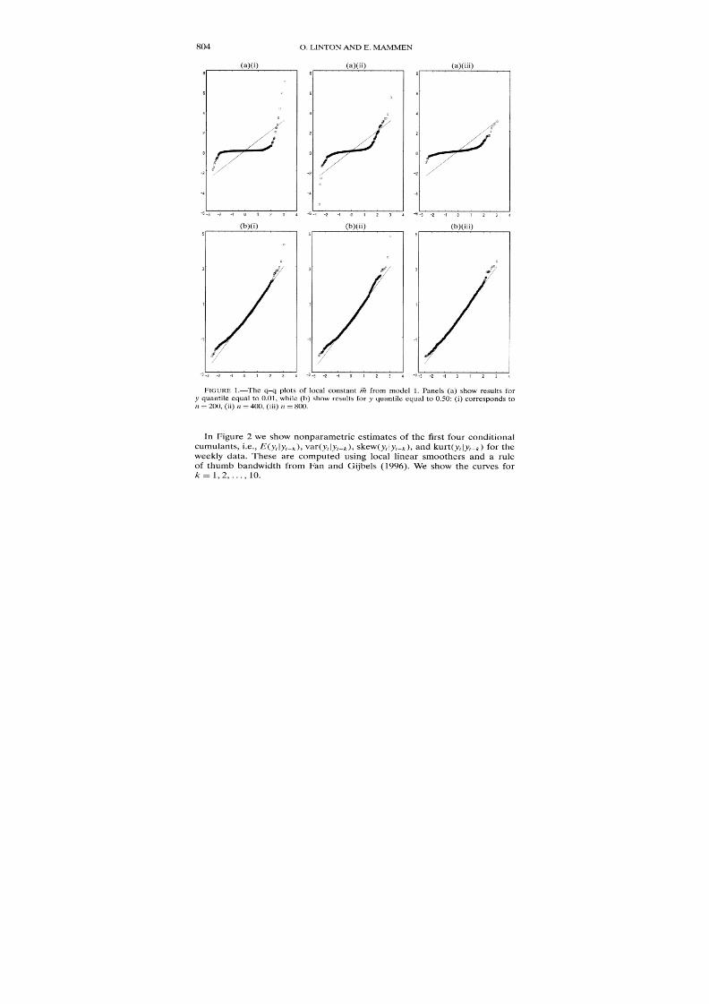
8/7/2019 Estimating Semi Parametric
http://slidepdf.com/reader/full/estimating-semi-parametric 35/67
0. LINTONAND E. MAMMEN
(a)(i)
D
o
a
(a)(ii)
-2
-4
-3 -2 -1 0 1 2 3 6 -3 -2 -1 0 1 2 3
(a)(iii)8 .
. . . . . . . .
6
4
2
-2
-4
-6 -3 -2 -1 0 1 2 3 4
(b)(i)
..
(b)(ii)13
0
-3-3 -2 -1 0 1 2 3 4 3 -3 -2 -1 0 1 2 3
(b)(iii)5 .
. . . . . I I I
3 /
1
/
-3-3 -2 -1 0 1 2 3
FIGURE 1.-The q-q plots of local constant ii from model 1. Panels (a) show results for
y quantileequal to 0.01, while (b) show results for y quantileequal to 0.50: (i) correspondston = 200, (ii) n = 400, (iii) n = 800.
In Figure 2 we show nonparametric estimates of the first four conditional
cumulants, i.e., E(y lyt_k),var(ytlYt-k), skew(yt ly_k), and kurt(ytlyt_k) for the
weekly data. These are computed using local linear smoothers and a ruleof thumb bandwidth from Fan and Gijbels (1996). We show the curves fork = 1, 2,..., 10.
804
-4
-6
a
5
3
5
3
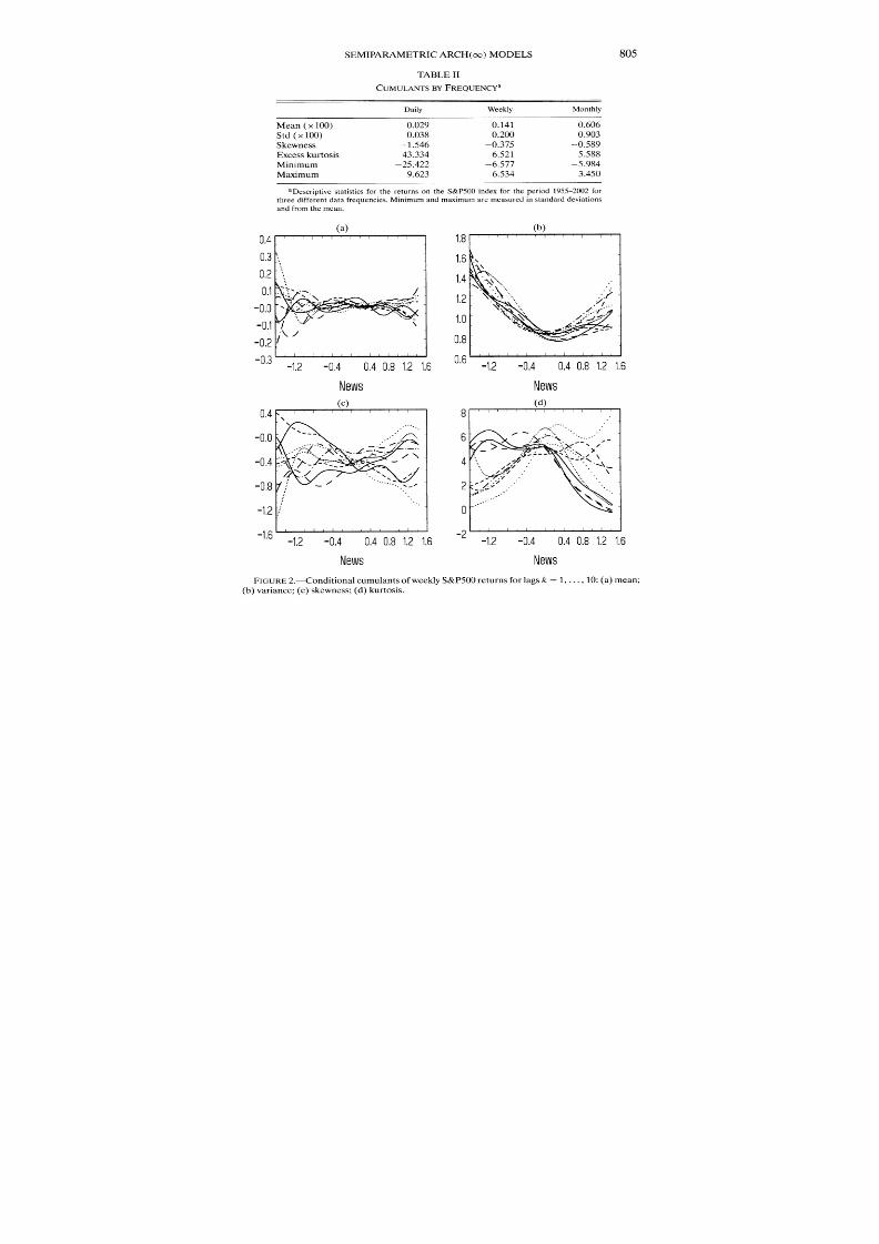
8/7/2019 Estimating Semi Parametric
http://slidepdf.com/reader/full/estimating-semi-parametric 36/67
SEMIPARAMETRICARCH(oc) MODELS
TABLEII
CUMULANTSBYFREQUENCYa
Daily Weekly Monthly
Mean (x100) 0.029 0.141 0.606
Std(x100) 0.038 0.200 0.903
Skewness -1.546 -0.375 -0.589
Excess kurtosis 43.334 6.521 5.588
Minimum -25.422 -6.577 -5.984
Maximum 9.623 6.534 3.450
aDescriptivestatisticsfor the returnson the S&P500indexfor the period1955-2002for
threedifferentdatafrequencies.Minimumandmaximumare measuredinstandarddeviationsandfromthemean.
(a) (b)
News News
-1.2 -0.4 0.4 0.8 1.21.6
News
-0.4 0.4 0.8 1.2 1.6
News
FIGURE2.-Conditional cumulantsof weeklyS&P500returnsforlagsk = 1,..., 10:(a) mean;
(b) variance;(c) skewness;(d) kurtosis.
-1.6
805

8/7/2019 Estimating Semi Parametric
http://slidepdf.com/reader/full/estimating-semi-parametric 37/67
O. LINTON AND E. MAMMEN
There does not appear to be much common structurein the conditionalmean.The conditionalvariancesaresignificantlydifferentfromconstants and
appear to have similarasymmetricU shapes. The conditional skewness andkurtosisare largein absolute value and have a varietyof differentshapes,withno common pattern,althoughthe skewness is mostly negative and the kurto-sis is mostly positive. Given the heavy tails in the data, these curvesmay notbe significantrelativeto the samplingvariability.Similarpatternsareobservedin the dailyandmonthlydata.Although there is no necessaryrelationshipbe-tween these marginalcurvesand the correspondingjointcumulantsE(y, 1F,_1),var(y, t_l), skew(yjlT,_), and kurt(y,lJ,_), this is suggestiveof a commonstructuresimilarto what is imposed in our model.
Following Engleand
Ng (1993)we fitted
regressionson seasonal dum-
mies, but, unlike them, found little significanteffects. In Table III we reportthe resultsof estimatingthe Glosten, Jegannathan,and Runkle (1993) model
(whichwe call GJR) parametricfits on these standardizedseries.All parame-ters appearsignificantand there is quite strongevidence of asymmetryat all
frequencies.We next applied our methods. We fitted an AR(2) process to the data and
then worked with the standardizedresidual series. We computed our estima-tors using r = 50 for the daily data and r = 25 for the weekly and monthlydata,where the dynamiccoefficientswere qj(0) = 0j-1 with 0 E (0, 1). We es-
timated the function m on the entire range of the data using local constant,local linear, and local quadraticsmootherswith variable bandwidthselected
TABLE III
PARAMETRIC ESTIMATIONa
Daily Weekly Monthly
P1 0.138788 0.007065 0.14661
(0.009524) (0.022000) (0.045131)
P2 -0.01906 0.051815 -0.018694(0.009449) (0.022044) (0.045083)
a(x 1,000) 0.0000721 0.00130 0.862000
(0.0000064) (0.000242) (0.249000)0 0.920489 0.850348 0.442481
(0.002243) (0.015580) (0.176365)7 0.034018 0.047885 -0.076662
(0.002613) (0.013504) (0.042047)6 0.078782 0.140013 0.266916
(0.003302) (0.020349) (0.094669)
aStandard errors are given in parentheses. These estimates are for the raw data series and
refer to the AR(2)-GJR-GARCH(1, 1) model
Yt = c + Pl Yt- + P2Yt-2 + t (Tt,
o2 = + 0-21 + yy_ + y22_l (yt-1 < 0).ut =a+ OoIt1
Yt1 11-(Y
806

8/7/2019 Estimating Semi Parametric
http://slidepdf.com/reader/full/estimating-semi-parametric 38/67
SEMIPARAMETRICARCH(oo) MODELS
3-
-8 -6 -4 -2 2 4 6 8
News
FIGURE3.-The bandwidthhT(y) used in the computationof mi(y) for the weeklyS&P500returnsdata.
by the rule of thumb (39) with the tail modification. Specifically,we choser(y) = exp(-(Iyl - 3)2) for ljy > 3. In Figure 3 we plot the bandwidth usedfor the computation of mi for weekly data as a function of y. For compari-son, the Silvermanrule of thumbbandwidthis 0.224,whichis smaller thanourbandwidthever is.
In Figure 4 we show our two semiparametricnews impactcurve estimates,
local quadraticMioand mi, along with the parametricalternative mGJRforthe three data frequenciesusingthe GJR dynamicparameters,denoted OGJR,
whichare takenfrom TableIII. Ourgraphsshowthe curves on the intervalde-fined by the 0.01-0.99 quantiles along with the standarderrors for the threeestimates. The main conclusions are the following: 1. There is evidence of
asymmetryfor daily, weekly, and monthly frequencies. 2. The least squaresestimators Mheshow the greatest growthon the negative side, while typicallylikelihood estimator m0 is a bit closer to the parametriccurve. 3. The min-ima of the curves in all cases occur on the positive side for each frequency.4. The
monthlymGJRis monotonic
decreasingon this
range,which is unex-
pected.105. The dailystandarderrorsobeythe anticipatedordering:the largest
l?Wehave recomputedthe parametricestimatesusingEviews,Gauss, and Matlab,but in allcases findqualitativelysimilarresults.
7 l l
807

8/7/2019 Estimating Semi Parametric
http://slidepdf.com/reader/full/estimating-semi-parametric 39/67
O. LINTON AND E. MAMMEN
(a)StandardErrors
0.24
0.20
0,16
0.12
0.08
0.04
I~~~~~~~~~
N /
0.0-3 -2 -1 0 1 2 3
(b)3.2
2.8
2.4 \
2.0
1.6 \
0.8
0.4
0.0-3 -2 -1 0 1 2 3
0.00-3 -2 -1 0 1 2
0.50
0.45
0.40
0.35
0.30
0.25
0.20
0.15
0.10
0.05
0.00
(b)
I .. .
v %O- ..
- -
\ /~~~~~~~~~~~~~~
-3 -2 -1 0 1 2
(c)
FIGURE4.-Estimated news impact curves for (a) daily, (b) weekly, and (c) monthly S&P500
returns along with standard errors in right panel. Solid line is mGJR; dashed line is ioGJR; dotted
line is naGJR.
are for iM0and the smallestare for mGJR.Both semiparametricstandarderrorsincreaserapidlywhen IyI> 2. The weeklystandarderrorsfollow a similarpat-tern
exceptthat the standarderrorsfor mi are
largerthanthose for Mi0when
y < -2.5. 6. The magnitudesof the standarderrorsare suchthat there aresig-nificant differencesbetween the news impactcurvesat variouspoints. 7. The
monthlystandarderrorsseem a bit erratic:the parametricones are too largeandthose for mi seemwaytoo smallwhen y > 0. 8. The tail partof the estima-
808
(a)Estmatorsof m
2.4
2.0
1.6
1.2
0.8
0.4
__ I I I
3
lo-'.1 ...
1% ,e .

8/7/2019 Estimating Semi Parametric
http://slidepdf.com/reader/full/estimating-semi-parametric 40/67
SEMIPARAMETRICARCH(oo) MODELS
-000-c
0
(00)U)z
0.86 0.88 0.90 0.92 0.94
FIGURE5.-S&P500 weeklydata.Negativeof log-likelihoodas a function of 0.
tion, which is not shown in the graphics,reveals quite substantialdifferencesbetween mGJR,m0, and mi. This is especiallyso in the dailydata where thereis a single isolated observationat -25 standarddeviations (the 1987 crash)and this forcesbig differences in the tail functions.Engle andNg (1993) foundsimilarresults.
We next estimated the full semiparametricmodel on the weekly data. We
took the dynamiccoefficientsto be Qj(0) = -l1, where 0 wasselected bya gridsearchon (0, 1) with width0.001;we computedmi andmi as describedabove.InFigure5we reportthe negativelikelihoodfunctionon the range[0.85, 0.95].The global minimumis at 0 = 0.899, which is slightly larger than the valueestimated in the GJR QMLE. The likelihood is a bit flat near the minimum
and, consequently,the standard error of 0 is quite large at 0.036, more thantwice the standarderror of the parametricestimator.The news impactcurvesare similarin shapesto those reportedabove and are omittedfor brevity.
Finally,we looked at some diagnosticsbased on the standardizedresiduals
t - yt/t, and t = Yt/at from the full semiparametrically estimated model,
weekly data. The conditional variances of these series show much less evi-dence of systematicshapes;the skewnesses and kurtosises are smaller in ab-solute value. We report in Figure 6 the correlogramfor the squaredresiduals
809

8/7/2019 Estimating Semi Parametric
http://slidepdf.com/reader/full/estimating-semi-parametric 41/67
O. LINTONAND E. MAMMEN
(a)0.20 ' , , , . .
0.15
0.10-
u_ 0.05 -. .............. .... ......
O -0.00 -
-0.05
-0.10
-0.15
-0.200 5 10 15 20 25 30 35 40 45 50
Lag
(b)0.20
0.15
0.10
o -0.00< .................. -............... ............ . ..- ..... ........ ........
-0.05
-0.10
-0.15
-0.200 5 10 15 20 25 30 35 40 45 50
Lag
FIGURE6.-Residual diagnosticsof estimatedsemiparametricmodelforweeklyS&P500data.
The estimated ACF alongwith95%Bartlettintervalsis shown(a) for and(b) for V.
2 and ; alongwith the Bartlettinterval?1.96/ T.1 There is verylittle evi-dence of autocorrelationin either series.
Ourapplicationhas confirmedsome of the findingsof Engle andNg (1993),namely the asymmetricnews impact curve, on the S&P500data set. We ac-
knowledge that we are not able to give a definitivestatement of the shape ofthe newsimpactcurve out in the tails,butourasymptotictheorybetterreflectsthisuncertaintythanthe theoryforparametricmodels,whichis overlyprecise.Thuswe are able to providea better idea of what we know we do not know.
7. CONCLUSIONSAND EXTENSIONS
Althoughwe have relied on the least squarescriterionto obtainconsistency,in practiceone can avoid least squaresestimationsaltogetherandjust applyaniteratedversion of the likelihood-basedmethod. We
expectthat the distribu-
11Itshould be noted that these confidence intervalsdo not take accountof the additionalvariationinducedbythe variousestimations;takingaccountof this estimationerrorwould widenthe confidenceintervalsconsiderably.
810

8/7/2019 Estimating Semi Parametric
http://slidepdf.com/reader/full/estimating-semi-parametric 42/67
SEMIPARAMETRICARCH(oo) MODELS
tion theory for such a method is the same as the distributionof our two-stepversion of this procedure. This is to be expected from results of Mammen,Linton,andNielsen (1999) andLinton (2000) in other contexts.
Other estimationmethodscan be used here like series expansionor splines.However, although one can obtain the distributiontheory for parameters 0and rates for estimators of m in that case, the pointwise distributiontheoryfor the nonparametricpart is elusive. Furthermore,such methods maybe in-efficient in the sense of Section 4.4. One mightwant to combine the series
expansionmethod with a likelihood iteration,an approachtaken in Horowitzand Mammen(2002). However, one would still need either to applyour esti-mation method andtheoryor to develop a theoryfor combiningan increasing
numberof HorowitzandMammen(2002) estimators.In the workingpaperversion we discusssome extensions of our method to
allow a model for the mean and some transformationmodels like logarithmicvariance,andpresent some ideas about"integrated"versions of ourmodel.
Dept. of Economics,LondonSchoolof Economics,HoughtonStreet,LondonWC2A2AE, U.K.;[email protected]
and
Dept. of Economics, Universityof Mannheim, L7, 3-5, 68131 Mannheim,Germany;[email protected].
ManuscriptreceivedSeptember,2003;finalrevisionreceivedNovember,2004.
APPENDIX A: PROOFSOF(8) AND(34)
In the sequel we take t, = 0 withoutloss of generality.
PROOFOF (8): It is convenient to break the joint optimization problemdown into two separate problems:first, for each 0 e 0, let mo be the func-
tion that minimizes (5) with respect to m e M; second, let 0, be the pa-rameter that minimizes the profiled criterion E[yt -
1E, rj(0)mo(yt_j)]2with respect to 0 E 0. It follows that 0o= 06 and mo = moo. We next findthe first-orderconditions for this sequential population optimization prob-lem. We write m = mo + e f for any function f, differentiate with re-spect to E, and, setting E = 0, we obtain the first-order condition E[{y2 -
EJ1 q)j(0)mo(yt-j)}{E=l 4l(0)f(yt-I)}] = 0, whichcanbe rewrittenas
00 00 00
(40) ij()E[Y2f(y- )] - Qj(0)lfi(0)E[m0(y-j)f(y_l)]j=1 j=1 l=l,j1 l
00
= ,2(e0)E[mo(y_j)f(y_-)]j=I
811

8/7/2019 Estimating Semi Parametric
http://slidepdf.com/reader/full/estimating-semi-parametric 43/67
O. LINTON AND E. MAMMEN
for all f. Taking f(.) = 8y(.), where 8y(.) is the Dirac delta function, we have
E[ylf(y-j)] = f E[y21yj = y']f(y')po(y')dy'
E[yoly_ = y']6y(y)po(y')dy'
= E[y y-j = y]po(y),
while E[mo(y-j)f(y-j)] = f mo(y')y(y')po(y')dy' = mo(y)po(y). Finally,E[mo(y_j)f (y_] E[E[mo(y_j)Iy_l]f (y_)] = f Emo(y_j)Iy_ y']Sy(y') x
Po(y')dy' = E[mo(y_j)ly_l= y]po(y). The next step is to changethe variables
in the double sum. Note that E[mo(y_j)ly_ = y] = E[mo(yo)lyj_- = y] by sta-tionarity.Let t = j - I. Then for anyfunctionc(.) defined on the integers,
E ? j(0)()O)c(j-
l)= E t+l(0)?l(O)C(t)j=l _l^,jl t-=?l 1=l
= 1 ~ ?,t+l(0)l(0) c(t).t=?:l /=1/
Therefore, dividing through by po(y) and l3 4i(0), (40) can be written
EJ=1 (0)E(y 1Y-j= Y) - EJ1 t (0)E(mo(yo)lj = y) = mo(y), which is thestated answer. Q.E.D.
PROOFOF(34): We writeg = go+ E f for anyfunctionf, differentiatewith
respectto e, and,settingE= 0, we obtain the first-ordercondition
r-1 2 1 1I d 2 I
Ed o~~ - : (Pjg0(Yt-j)=Ft2d9Ef E f(Yt) =0-
j =1 t l=1
whichcan be rewritten
t=1 - - 1-
00 00
- E ji/iE[?-'4go(yt-,)jyt- = y]lj=1 1=1,j li
Now use the law of iterated expectations to write E[ot,4go(y,_j)lytl = y] =E[E[t-41yt-j, yt-l]go(yt_j)lyt_l= y]. Then
E[ot 4go(t-j)lyt-l =y] = qj,(x, y) go(o,)po(x) dx,PoW(y)p(x)go(x)pW(x)dx,
812
8/7/2019 Estimating Semi Parametric
http://slidepdf.com/reader/full/estimating-semi-parametric 44/67
SEMIPARAMETRIC ARCH(oo) MODELS
where qj, (y, x) = E[ot-4 yt_j = x, Ytl = y]. The result follows. Q.E.D.
APPENDIX B: PROOFS OF THEOREMS
PROOFOF THEOREM1: We first outline the approach to obtaining the as-
ymptoticpropertiesof mi0(')for any 0 E0. We give some high level Assump-tions A4-A6 under which we have an expansion for me - me in terms of
i - m and H - 0.Both termswill contributea bias and a stochasticterm
to the expansion.We thenverifytheAssumptionsA4-A6 andverifythe central
limit theorem.
ASSUMPTIONA4: Suppose thatfor a sequence 8r -- 0, supoe,EimIl=l,xIcI- ox
m(x) -Hm(x)l = Op(ST)
In particular, Assumption A4 gives that suPoEo,Iml2=j1 1[H0- H0]m112=
Op(8T). We now show by virtue of AssumptionA4 that (I - H0) is invertible
for all 0 E0, withprobabilitytendingto 1, andit holds that (see also (14))
(41) sup I[(I-
o)-- (I- eo)']m(y) = Op(rT).
0E@,1m112=1,llI<c
In particular, supoeo,im12=1 [(I-FI)- - (I -0)-]mll2 = Op(Sr). For a proof
of claim(41) note thatfor m EMc,
00
m = (I -)-1[( -)- [('Ho- N0)(I - 0)-]'m
j=o
because of00
[(H - Ho)(I - )-] = [I -(I
- o)(I - -]-
j=o
= [(I-H)(I-Heo)-l]-
Thisgives
00
(I - HO)- m-(I- Ho)-m = L[(No - Ho)(I- Ho)- 'm.j=0
We suppose that Mi`(y)has an asymptoticexpansionwhere the componentshave certainproperties.
813

8/7/2019 Estimating Semi Parametric
http://slidepdf.com/reader/full/estimating-semi-parametric 45/67
0. LINTON AND B. MAMMEN
ASSUMPTIONA5: Suppose that with 8T as in Assumption A4, Miii(y) -'_*'*DB *,C, ndY-*,D B tm*(y) = jB(y) + j$4C(y) + jlD(y), where Dsatisfy
(42) sup pih*B(y)I-OT(T 25) withjj detenninistic,OEO,IyI<C
(43) sup '*'C(y)J =Op(T2156T1),OEO,Iyl<C
(44) sup 7iH(I- 7-(o)-'l*,C(y)j =op(T 2 5)EO, Iyl<C
(45) sup Jjj*,D(y) o (T-2/5)0C0,Ijy<C
Here, M.*,Bis the bias term, MOLCis the stochastic term, and MIODis the re-
mainder term. For local linear estimates of gj(y) it follows that under standard
smoothnessconditions,(42), (43), and(45) hold.The argumentis complicatedby the fact that Mi'depends on a large number of gj(y)'s, although it effectivelybehaves like a single smoother. The intuition behind (44) is based on the fact
that an integral operator applies averaging to a local smoother and transforms
it into a globalaverage,thereby reducingitsvariance.Define now for
j= B, C,D the terms
M.iias solutions to the
integral equa-tions Mi- = "M + o M'sand M',''implicitlyfrom writingthe solution m0 + M"A
to the integral equation
(46) (m6?ii%=mO ?7-(O(mO + MOi).
The existence and uniqueness of Miuifollows from the invertibilityof the op-erator I - '-Ho(at least with probabilitytending to 1). It now follows that
o= mo+ MO+ M- O MO+ by linearityof the operator (I - H-Oe)`1.Note
that jj =J - 7-(o) M'i7i,forj = B, C, D, while m6?M_ = (J - -) 'm. De-fine also mB as the solution to the equation
B BB(47) MO= mO + 'LOM
We now claim that under Assumptions Al-A5,
(4i8) sup I-B (y)_MB(y) I=o( -25),(48) MO\Y -Yn = p(T-j,0EO, 3'!<c
(49) sup Ii,(y) c- -,*,C(y)l= op(T 25)OEO, yj<c
(50suI i( =y=o -2/25).sup MpcOEO,IYI<C
814
(50)

8/7/2019 Estimating Semi Parametric
http://slidepdf.com/reader/full/estimating-semi-parametric 46/67
SEMIPARAMETRIC ARCH(o) MODELS
Here, claims (48) and (50) immediatelyfollow from (14) and (41). For (49)note that because of (43)-(44), (41), and Assumption A4, supOE,,yl<c1H,(I -
Ho)-' *C(y)l = Op(T-2/5). So we arrive at the expansion of m0:
sup iJo(y) - mo(y) -m (y)- mB(y ) - m (y) = o(T-2/5).OEO,yl<C
This gives an approximation to mie(y) - mo(y) in terms of the expansion of m ,
the population operator Ho, and the quantityiA(y). This latter quantityde-
pendson the randomoperatorHe.Next we approximatethe quantityMiA(y) by simplerterms. By subtracting
mo = m*+ Homo
from(46)
weget mi
=(HO
-Ho)mO
+HOMiA.
We next
write1Hoas a sum of terms with convenientproperties.
ASSUMPTIONA6: Suppose that for 8T as in Assumption A4, (He - Ho) x
me(y) = E(y) + mF(y) + m,G(y), where ME, IO , and m*G satisfyI'*,E(y) -2/5 *,p ,
supoeo,jyl<c m*,E(Y)I= Op(T-2 5) withm*E deterministic,supM,,0,yl<Im, F(y)l =
Op(TT-2ST ), SUP,eiYJ<C1(I - moH)-F(y) = op(T-2/5), and
supo yl, JiG(y)l = o (T-2/5)
Again, m ,Eis a bias term, m* is a stochastic term, and m-*,Gis a remainderterm. For kernel density estimates of Ho under standardsmoothness condi-
tions, the expansioninAssumptionA6 follows from similarargumentsto those
given for AssumptionA5. Define for j = E, F, G the terms mJ as the uniquesolutions to the equationsm' = iM,j+ Homi. It nowfollows thatm can be de-composed into mA = +mE + + mG. Define m0 as the solution to the second
kind linearintegralequation
(51) mE= m-- omE
As abovewe get that
sup Im-E(y)-mE (y)= op(T-2/5),OEO,lyl<c
sup ImF(y)- ,F(y) ( 2/5), andOEO,IYI<C
sup m(y)l =op(T-2/5).EO,Iyl<c
We summarizeour discussion in the followingproposition.
PROPOSITION1: SupposethatAssumptionsA1-A6 holdfor some estimatorsAMand H. Define im as anysolutionof mi = m + Home.Then thefollowingmo
815

8/7/2019 Estimating Semi Parametric
http://slidepdf.com/reader/full/estimating-semi-parametric 47/67
O. LINTON AND E. MAMMEN
expansionholdsfor mii:
(52) sup meH(y)- m
(y)- m(
(y)-
mC(y)-mM
(y)0EO, 1'1<c
= o(T-2/5)
The termsmB and mEhavebeendefinedin (47) and (51), respectively.
Equation (52) givesa uniformexpansionfor mio(y)- mo(y) in terms of a de-terministic expression mB(y) + mE(y) and a random variable m,c (y)-+mi(y)o,l 11111113L1, ArlL?3~1VII,Imo(Y + m(Y)that is explicitlydefined. We have hithertojust made high level assumptionson mOand the operator 'Hoin AssumptionsA4-A6, so our result applies to
any smoothingmethod that satisfies these conditions.It remains to provethatAssumptions A4-A6 hold under our primitiveconditions B1-B7 and that acentral limit theorem (and uniform convergence) applies to m,c (y) + imiF(y).
PROOFOF HIGHLEVELCONDITIONSAl, A3-A6, ANDCLT: We first define
the conceptof near epoch dependence (NED) for stationaryprocesses,whichwe will use in the sequel.
DEFINITION:The stationary process {x } is said to be stable (NED) in
L2-normon the stationarya-mixing process {zt } if there exist measurablefunc-tions g, suchthat,as m -- oo, v(m) = E[Jxt- gm(Zt-1, . .. , Zt-m)12] - 0.
This definition provides a sufficient condition for the more general NEDdefinition in say Andrews (1995). The process o-2(0)= J=I f(O0)m(y,_j)is
stable in L2-normon the process {m(yt)} (which is a-mixing) and the sta-ble numberssatisfyv(m) < exp(-cm) for some constant c > 0. Likewise,theprocess rtt is geometrically stable on {y2}and 7t is geometricallystableon {me(yt)}. We use this property below.
AssumptionsAl and A3 follow
immediatelyfrom our conditions on the
pa-rameterspace anddensityfunctions. We assumedAssumptionsA2 in B7.We verify Assumptions A4-A6 with the choice 8T = T-3/10+ with s > 0
small enough. This rate is arbitrarilyclose to the rate of convergenceof two-dimensional nonparametricdensity or regression estimators. We will verifyAssumptionsA5 and A6 with
m*0B(y = 2U2(K) x /O(Y), MC(y)
T-TT
)YK ,(y, -Y)r78,t,mo(Y)Tpo(y) L=l
h22 2(K) x 13(y),
2
816
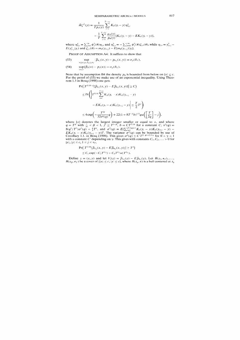
8/7/2019 Estimating Semi Parametric
http://slidepdf.com/reader/full/estimating-semi-parametric 48/67

8/7/2019 Estimating Semi Parametric
http://slidepdf.com/reader/full/estimating-semi-parametric 49/67
0. LINTONAND B. MAMMEN
of radius E, while Q(T) is a sufficientlylarge integer and Q(T) = 2c2/ET. Bythe triangle inequality,
Pr sup Vj(z)I > 2c8T
<Pr max (Zq) I > C8TI<j<7
1<q<Q
?Pr max sup jJj(Zq) Vj(Z)I > C6T
-1j,7 ZeB(Zq,ET)
1<q Q
for any constant c. By the Bonferroni and exponential inequalities,
- T Q
Pr max lJj(Zq)l >C8T ( CPr[/l4zq)I>>c8T<]i<j<T
:P[IV Z)I>CT
I<q<Qj 1 q=I
< QT[CI exp(-C2Tc3) + CjTCSa(TC6)]
= o(l),
provided so in Bi is chosen large enough. By the_Lipschitz continuity of K,
lKh(Yt- x) - K,(yt - xq)J < Kix - xqllh, where K is finite, and so T'310 f x
lj(Zq) - V(z)I < T'1105(1/ h24c[Ix - Xqi+ C21Y- Yqll <CETT7/10-5
for someconstants cl,C2. This bound is independent of j and uniform over z, so
that provided ETT711-* 0, this term is o(1). This requires that Q(T)/710
We have given the detailed proof of (53) because similar arguments are used
in the sequel. Equation (54) follows by the same type of argument. Q.E.D.
PROOFOFASSUMPTIONA5: Claim (42) immediately follows from assump-tion B4. For the proof of (45) we use the usual variance + bias + remainder
term decomposition of the local linear estimates'
as in Masry (1996). Write
M(y) = po(Y) diag(1, c2(K)) and
MTJ(y)=]jhEKYh-Yt-)j t (YYth1 h~~~~~~~~~~~~~
t~~~~~~l(X )2
Then'
(y) - gj(y) = B, + whereB eM )BT(y), andBTj(y) is agj jy ~~~~~~~~~~1TjYY/)j\ ii 7'\ 3C
vector BTj(y) = [BT1,o(y), BTj I(y)]T, where
BTJI(y)= ThL(h:
)K(Ii-y
t I
818

8/7/2019 Estimating Semi Parametric
http://slidepdf.com/reader/full/estimating-semi-parametric 50/67
SEMIPARAMETRICARCH(oo) MODELS
where Agt(Y)= gj(y,-j) - gj(y)(Yt-j - y) = g(y*j)(yt_j - y)2/2 for some inter-
mediatepoint Y*j.The varianceeffect is Vjy= e'MT- (y)UTj(y).The stochastic
term UTj(y) is UTj(y) = [UTj,(y), UTj,l(y)]T,where
We have m*o(y)- m*(y) = Ejt J(O)[gj(y) - gj(y)] - Yj=+l (jt()g
j=l =1
Wethenuse thesupfactthatI supY<c<+Tlj(y) ) -c(y)'+ = o(), whichfol-o
lows by thesaminite ronstantc as for (53) and (54). Defining and B as
fore,
Vjyand Bjywith MTj(y) replaced by M(y), we have
T T
mo(y)- m*(y)= Y jt(0)VjyI+ o,(0)Byj=1 j=1
+ RT(y, 6) + RT2(y, 0) + Op(T-1/2),
T
whereRT1(Y,6) j= j(0)[Vjy- Vjy]andRT2(Y,0) = Ej=i j(0)[By-Bjy]
Wehave
j=1 j=1 t=TT+l
T T-TT Kh(Y- ys)r7j,s
T-TTKh(y-Ys) 1j(O)j,s
s=l po(y)Ts--
T-TTKh(yt- y)rl,t (- y),t
t1 po(y) Tpo(y)
by changing variable t t- t - j = s and interchanging summation.
819

8/7/2019 Estimating Semi Parametric
http://slidepdf.com/reader/full/estimating-semi-parametric 51/67
O. LINTON AND E. MAMMEN
We show that
(55) sup IRTl(y, 0)=
Op(T-2/5),yI<c, OEO
(56) sup RT2(y, 0) = Op(T-2/5),lyl<c,ECO
1T-TTK
(57) sup Kh(y,- y) j(0)j =op(T-2/5).\yjC6 EOTpo(y)
T +l
t=1 j=r+l
It follows that
m(y) - m(y)
T-rT T
=Tp (y) LEKh(Yt-Y),+ E (Bj + op(T-2/5).Tpo(y)t l
t=l j=
We establish next (57). Define T, = T-1 E TT Kh(yt - y) EjOT1 f(6)mI,t/po(y). First note that E(Tn) = 0 and
T-TT T-TT o? cx
var(T2) ()E E E E j(O) (O)E[KtK,,s tr,s]T27 2p(y),h21 T+l+PO
+ t=1 S j7 1s=l
< CI
-CTh2(1-ll)po(y)
oc oo 00
~xE ^,;j(0) ,(0) a(j-(S +/ ))l-l12p
j=T+=+l s=l
- Thl_I/2(2T+I) o(T-lh-1)
by Davydov's inequality, the mixing condition B1, and the decay condi-tions B10. Here, Kt = K((yt - y)/h) and C, C' are generic finite constants.
This establishes the pointwiserate of T,,.The uniformityof the bound in (57)can be achievedby applicationof the exponential inequalityin Theorem 1.3of Bosq (1998) used also in the proof of (53). The proofs of (55) and (56) aresimilar.
Forthe proof of (43) we applythis exponential inequalityto bound
PrT2/5 Kh(yt -y) 7o,)
> T3/1+t=l Po(Y) 2
820

8/7/2019 Estimating Semi Parametric
http://slidepdf.com/reader/full/estimating-semi-parametric 52/67
SEMIPARAMETRIC ARCH(oo) MODELS
where 0T,t= Ejt1 J(0)[min{y2+j,T'/P}-E(min{y2+j, T1/P}lyt)].The truncated
randomvariables o,t can be replaced by eo,tusing the fact that 1 - Pr(y2<
T1IPfor 1< t < T) < TPr(y2> T/)
<
E[yt2i(y2> T/)] ->0.It remainsto check (44). Define the operator C?(x,y) by oe(I- H)-~ x
m(x) = f CcL(x, y)m(y)po(y) dy. The LC(x,y) can be constructedby use ofthe eigenfunctions {eo,j)l1 of -0.Denote as above the correspondingeigen-values by Ao,j.Then
00
'O(x, y) = LAo,jeo,i(x)eo,j(y) and
j=l
A00 ,
o(X, y) = e ,j(x)e,j(y).1
-Ao,j
Note that for a constant0 < y < 1we have sup0o,,>lA0,j< y. This shows that
L2(x, y)po(y)po(x) dx dyc
00 A2 1 0
L( jl< A2 < 00.
?= (1-Ao,j)2 - (1 y)2 = aj
Furthermore,it can be checkedthat L?(x, y) is continuousin 0, x, y. This fol-lows fromAssumptionA3 andthe continuityof -Ho(x,y).
Therefore, we write Ho(I - -o)-lmi'c(x) = ET Ivo(t, x)r1 with
vo(z, x) = fSC (x, y)(l/po(y))Kh(z - y) dy. The function vo(z, x) is contin-uous in 0, z, x. Using this fact, claim (44) can be easily checked, e.g., againby applicationof the exponential inequalityin Theorem 1.3 of Bosq (1998).
Q.E.D.
PROOF OF ASSUMPTION A6: Write
'HF(y,x)me(x)po(x) dx - 0(y, x)mo(x)po(x)dx
+7TfT - o,j (y, x) Po0,1(Y, x)
=-Lvj>o)f mo(x)dxi=? J po(y) Po()
?rT
?+ L (0)(Po(y) P-Po(wY)) i(Y,X) mo(x)dx
+ i-Po(T(y)j=+tlP
- op(T -2/5).
821

8/7/2019 Estimating Semi Parametric
http://slidepdf.com/reader/full/estimating-semi-parametric 53/67
O. LINTON AND E. MAMMEN
Using this expansion one can show that mi,G(y) = (t -t (y) -
moF (y) is of order op(T-2/5). The other conditions of Assumption A6 can be
checked as in theproof
ofAssumption
A5. Q.E.D.
PROOFOFCLT FORm4'C(y) + MiF(y): This follows by an application of a
centrallimittheoremfor triangulararraysof NED processes alongthe lines ofLu (2001).The argumentis firstto replace,forexample,7I, bythe logarithmictruncation t'tJ= j= O(0)rj, t. Then divide the sum t=1 Kh(yt - y)rl t into
the usual Bernstein large block/smallblocks. Then applyDavydov's inequal-ity for random variableswith finite p moments. Because of the exponentialdecline of the stabilitynumbers v(m), the CLT follows. This concludes the
proof of (26). Q.E.D.
PROOFSOF (27) AND(28): The only additionalityhere is to show that
SUP0e0il< I4C(y) + m *F(y)l = op(T-l/4). This followsby applyingthe expo-nential inequalityagain.
Finally,
sup la,2(0) _-2(60)0,l<t
00
< sup j(0) sup Iie0(y) - me(y)0 0,lyl-<c
oo T
+sup E Ij(0) supm o(y)+T Eym - E[y2]j=r+l
lY< t=1
< _ sup ImO(y)-mo(y)l + +1supme(y) + Op(TrT1/2)1 -
I ,lyl_<c lyl<c
=op(T-1/4)
bythe summabilityconditions on qj(0), the boundednessof mo(y) on [-c, c],and the uniformconvergenceresult (27). Q.E.D.
PROOFOF THEOREM2: Consistency. We apply some general results for
semiparametric estimators. Write ST(O) = T-1 jT=Yyt - -o2(0)}2, where
oa2(0)= E'j Qj(O)mo(yt-j), and let S(O)= EST(0). We show that ST(0) -
S(O) = op(l) by applying a law of large numbers for near epoch depen-
dent functions of mixing processes. Let m(y) = supoE mo(y) and me(y) =supoEl Idmo(y)/ldOel,which are bounded continuous functions on [-c,c].It follows that sup,,,2() < Cj i-'m-(yt_j) and sup0E Iodf(0)/d0l <
C =l J-'(m(yt-j) + me(y)), which are both bounded processes. Therefore,
822
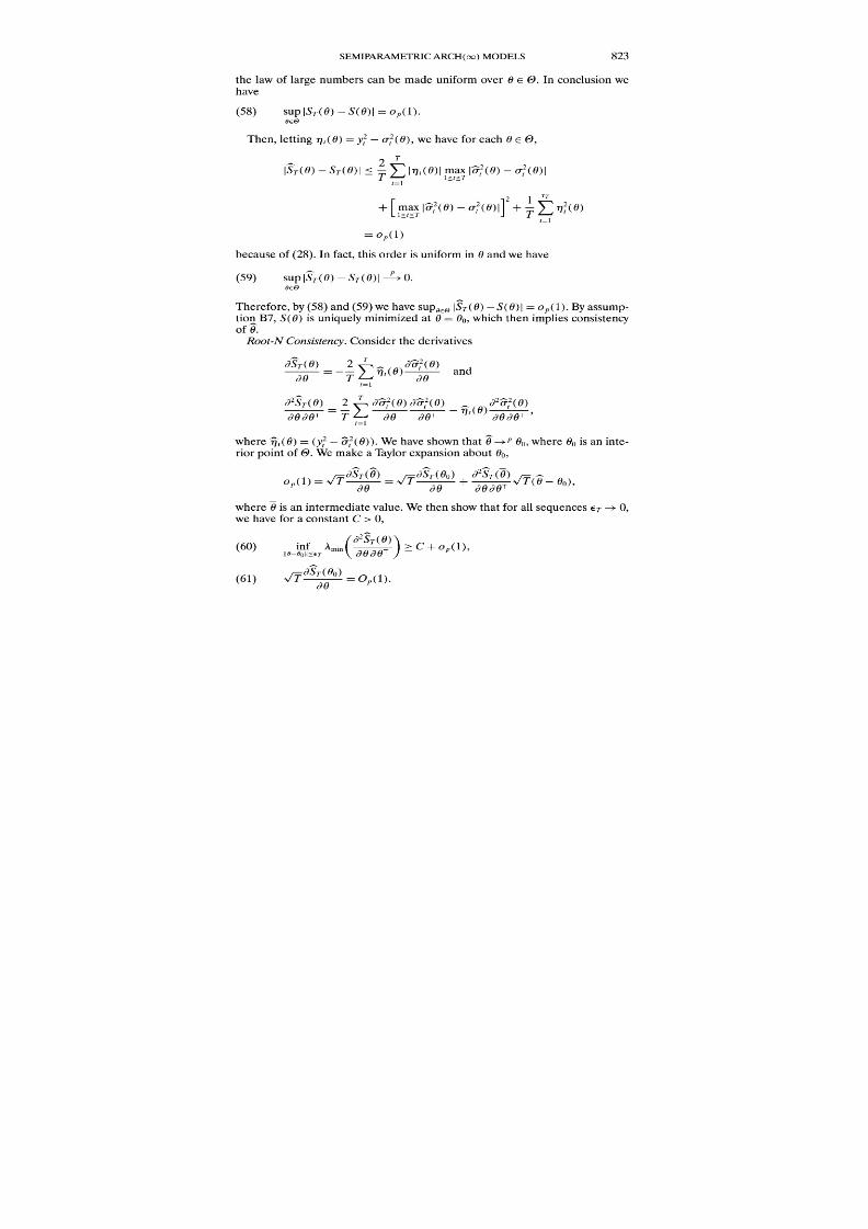
8/7/2019 Estimating Semi Parametric
http://slidepdf.com/reader/full/estimating-semi-parametric 54/67
SEMIPARAMETRICARCH(oo) MODELS 823
the law of large numbers can be made uniformover 0 E0. In conclusion wehave
(58) sup IST(O)- S(0) = Op(l).0EO
Then, letting r/(0) = y, - ot2(0), we have for each 06 0,
ISr(0) -STr(0) _< T I(0)max 2(o0)
-r2(0)1
t=l
2 1TT
+[maxlatT2()
-(t(0)]+ 2(T0)
l1<t<T T
(Ot
t=l
= op(l)
because of (28). In fact, this order is uniform in 0 and we have
(59) sup IST(0) - STr()I 0.0EO
Therefore,by (58) and(59) we have supGOEIST(O)- S(0)I = Op(l). Byassump-tion B7, S(O) is
uniquelyminimizedat 0 = 00,which then
implies consistencyof 0.Root-NConsistency.Consider the derivatives
ST(0) Y2r o (0 ) andO0 -rE 7 dt(0) and
d2ST(0) 2 d3t2(0) dt2(0) 2 2 (0)
dOdTT T 860 dO0T 6t0T 't=l
where t(0) = (yt2- at2(0)). We have shown that --P 00,where 00 is an inte-riorpoint of 0. We make a Taylorexpansionabout 00,
O /ST (O)d/ST (00) ST --( -P( dOde dOdTe AT(d)0
where 0 is an intermediate value. We then show that for all sequences 0,we have for a constant C > 0,
(60) inf Amin(>dT) >C + op(1),1 II-001-<ET T /-
C+ '
(61) v-T=SO( ) ).86 O()

8/7/2019 Estimating Semi Parametric
http://slidepdf.com/reader/full/estimating-semi-parametric 55/67
824 0. LINTON AND E. MAMMEN
This impliesthe N/Tconsistency.To establish the results (60) and (61) we use some expansions given in
Lemma1.
PROOFOF(60): By straightforwardbut tedious calculationwe showthat
92ST(0) 82ST(O)sup =op(l).
110-o001<ET,l'<t T 0 0T dO0 0T
Specifically,it suffices to show that
d c^r2(0) d?2y(0)
sup
( -d
O((l),11-0011<T,l<t<T dO0j 0 J
j 0, 1, 2. Forj = 0, 1 this followsfrom(28) and(29). Forj = 2 this followsbysimilarargumentsusing Lemma 1. Note also that by B4 for a constant c > 0,
inflo-I< ET,1<t<T of2(0) > c. Furthermore,
2(ST(0) (o-t2(00) o-t( 00)sup -E = op(l)
10o001 <-E TdO0Td.. 80 80T
by standardarguments.Therefore,bythe triangle inequality,
o2ST(0) arr2(0o)dt =2(0 o)sup -E =op(l).
le0-0OlleT< ' T d6O d0 T _ Q.E.D.
PROOFOF(61): Write
sT(0o)[ 2
T
d 0)T -Y - C2(0 o) - [t (00) - (0)]]
t=l
-
o-t(0o) + ^2(0o) o 2(0o)x -0dO dO dO
and let with 7lt = ql(00), xTET(00) = ET1 + ET2,
1 T dcr2(00)ETI= 1 T)-C0()]
t=l
T ot(00)La(0o) -
80ao
1T - a2 (0o) _27(Oo)--
t=- 88l -t=1~ ~ ~ d
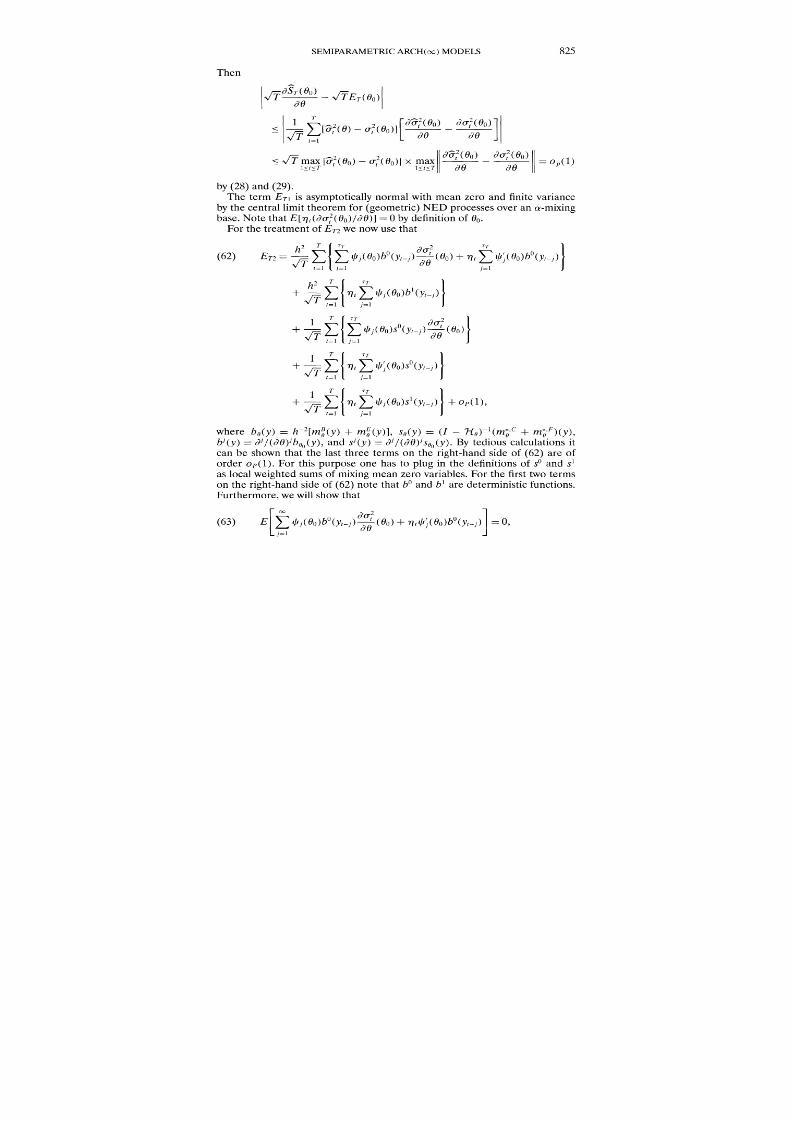
8/7/2019 Estimating Semi Parametric
http://slidepdf.com/reader/full/estimating-semi-parametric 56/67
SEMIPARAMETRICARCH(oo) MODELS
Then
/ST (0B )_ ET ( o)
1 -T 8a2(0) doto(0o)< (7- 07(Oo)] d C82 d_/-rt= l
<V max l'(00) -o-7(00)1
x max d (0) - d-(00) (1)<t<r i<t<Tr 86--
by (28) and (29).
The term ET1 is asymptoticallynormal with mean zero and finite varianceby the central limit theorem for (geometric) NED processesover an a-mixingbase. Note that E[-rt(S-rr(0o)/,0)] = 0 bydefinitionof 00.
For the treatmentof ET2we nowuse that
h2 TJ'?T o2 IT
(62) ET2 = /- l- E jV(0o)b?0(yt-j) (0) ) + t; E t(0 o)b(yt-j)
"'+',3 E Tit E ?J(O?)b~(Y'-J)
1 da ~ 1+-E | E 8j(uo)sO(y 2_j)._.(_(o)
t=l =i j= l
'2'-2 t T
+ -7tN/T L, | t E J(0o)s (yt-j)
Vt'=1I yj=l
tr(=11 /=1? E7L t EL j((o)s (Yt-j) + Op(l),
where bo(y) = h-2[m(y) + mE(y)], so(y) = (I - o)- (m + mF)(y),
bj(y) = di/(80)Jibo(y), and sJ(y) = d8/(d0)Isoo(y).By tedious calculations itcan be shown that the last three terms on the right-handside of (62) are oforder Op(l). For this purpose one has to plug in the definitions of so and s1as local weighted sums of mixingmean zero variables.For the first two termson the right-handside of (62) note that b?and b1are deterministicfunctions.
Furthermore,we will show that0o dnot2
(63) E by j(0o)by-- (0o)t (H) +0 rltY(0o)b (yt-j) = 0,_-j=l _u- j=1
825

8/7/2019 Estimating Semi Parametric
http://slidepdf.com/reader/full/estimating-semi-parametric 57/67
0. LINTONAND E. MAMMEN
00
(64) E mLV j(6o)b'(ytj) =0.- j=1
Note that in (63) and (64) we havereplacedthe upperindex of the sumby cx.
Thus, with (63) and (64) we see that the first two terms on the right-handside of (62) are sums of variableswith mean geometrically tending to zero.The sums are multipliedby factors h2T 1/2* By using mixing propertiesit canbe shown that these sums are of order Op(h2) = op(l). It remains to check
(63)and(64). Bydefinition for eachfunctiong, E[r{y- \L\ Ifj(0)3g(yt_j)12]
is minimized for 8 = 0. By takingderivativeswith respectto 6 we get that
(65) E{[yt- o-t7(0)]L(1 0(()g(yt-j) =0.
Withg = bo and Oothis gives (64). For the proof of (63) we now take the dif-ference of (65) for 0 and 00.This gives
00
E[y2- o7(o2)]L[YI'(6) i/iij(0o)]g(ytj)j=l
- E[oQ(0) - o7(Oo)] Lq1(0)g(yt ) = 0.
j=1
Taking derivatives with respect to 0 gives Er,Jut qY0o)g(yt_j) - dot/
dO(00)Co qjij(0o)g(yt-j)] = 0. With g = bo this gives (63). Q.E.D.
PROOFSOFTHEOREMS3 AND 4: We only give a proof of Theorem 3. The-
orem 4 follows along the same lines. For a proof of (31) one shows that for
C > 01 SUP110-001ICT-12IMii0(y)- 6i60(y)l= op[(Th)1/2]* This claim follows by
using appropriate bounds on Ho(e- 7oo and i-` - Mi-oBecause of (31), for a proof of (32) it suffices to show
(66) z/Th[Mo0(y) - moo(y) - h2b(y)] ==i N(0, w(y)).
So it remains to show (66). Put f\(y) - T 1 (Yt - y)Kh(y1 - y) and
)^0(y) = T-1jsTI (yt - y)2Kh(yt - y). Then, by using similarargumentsas in
the proof of Theorem 1, we have for y > 0, suplyl,I)%(y) - h=2AAK)p (y) I
826

8/7/2019 Estimating Semi Parametric
http://slidepdf.com/reader/full/estimating-semi-parametric 58/67

8/7/2019 Estimating Semi Parametric
http://slidepdf.com/reader/full/estimating-semi-parametric 59/67

8/7/2019 Estimating Semi Parametric
http://slidepdf.com/reader/full/estimating-semi-parametric 60/67
SEMIPARAMETRICARCH(oo) MODELS 829
-p, (y) I 1 1=h2A2(K) ml/ 'H^y} p(T-12).=h2/,2+(K) mP? O (Y)m o -( jem0(y) + o(T /2)
_Po(Y) 2 2
Therefore we get uniformlyin IyI< c,
moo(y) - moo(y)
= (I- Ho,)-1[mo (y) - (I - Hoo)moo(y)]
= (I-1O)1[mo ) --0)m-(y)-( - ) ()] + op(T-/2)
= 1TVtr (6 )VKh (Yt--
Y) 2
-Too90'
4.,}^ ptut
t=1 -_i= 1o(Y)
+ h2. 2(K)(I- _H0o)-1
x ( P -(y o0mo(y) - mo(y) + )YoOmo(y)
,2 2
mo (y) m ' (Y)+- ( )
m~ (y)7"{oomP (y)
+ o (T-1/2)
with K*= ET1 j(0o)Kh(yt-i - y)/po(y). Fromthis stochasticexpansionwe
immediately get an expansionfor the asymptoticbias. For the calculationof
the asymptoticvariancenote that
hEK*2=h 2 0(o)/(0o[)E{Kh(yt - y)Kh(yt- - y)Po(y) j5
xE[o-tul\yt_j, yt]}
00
+(0,o)2E{KI(yt
- y)E[4t_y =
y]}j=1
+ v2 o(K) uf(o)2E(ou-42ytj = y) + o(1)Po(Y)1Y
j=1

8/7/2019 Estimating Semi Parametric
http://slidepdf.com/reader/full/estimating-semi-parametric 61/67
O. LINTON AND E. MAMMEN
O(30-- 00
p(Y) E / (0o)2 vo(K) E j(j(O)2E[o-tu \yt j =y]po(y)
_: _: Po
()- j=1
+o(l). Q.E.D.
PROOFS OF THEOREMS 5 AND 6: The proofmakes use of similarargumentsas in Theorems 1-4. For this reasonwe only give a shortoutline. We firstdis-
cussmi. Belowwe will showthat 0- 00= Op(T-1/2). This canbe used to show
that suplyl< Ii00(y) - m(y) = op(T-2/5). Thus, up to firstorder the asymptot-
ics of both estimatescoincide. We comparemiiOwith the followingtheoretical
estimateme.
Thisestimate is definedby
theintegralequation
me =m0 +7 mo,where
m*= _ Ej L ((1 ()1j(o)J(Y)m?
~(Y) b7=y0
J/j (0)gj(Y)
=l,l j i(j) 1( ) gi, j (X, Y)Po (c y)
0qg(x, ) TT 2 (0)P(y)
Ej=Zi O)gj(Y)
Here ga is the local linear smooth of o- 4y2 on Yt-j,gb is the local linear fitof 't-4 on yt-j, andg,j is the bivariatelocal linearfit of ot-4 on (Yt-l, t-j). Note
thatgj, g', g are defined as , , j, but with -r2replaced by o-2.Further-
more, mo is defined as mebut with j, g, ,j replaced by g, g, g.
By tedious calculationsone can verify for a constant C > 0 that there ex-
ists a bounded function b such that uniformlyfor lyl < c, 110- 00lo CT-1/2,
mo(y) - m(y) - h2b(y) = op(T-1/2). The bias term b is caused by bias terms
of 7- a,2.So up to bias termsthe asymptoticsof mo(y) andmie(y)coincide.
The estimate meo(y) can be treated as mo0(y) in the proof of Theo-
rem 3. As the stochastic term of moo(y) we get T-'ly =Kt(y)o' 4(y -
or2) = T-1 l Kt(y)ot 2ut, where Kt(y) = ETi j(0Oo)Kh(y-y- y)/Po(y) x
TT1j2(Oo)E[otly,t-j = Y].Asymptoticnormalityof this termcan be shownbyuse of centrallimit theoremsas in the proofof Theorem 1. For the calculation
of the asymptoticvarianceit can be easilycheckedthat
1v(r)Ej=I 2(oj -41 y)hE[Kt(y)2 42] =14 11 2
(0o)E(u4a)Po(y) [ l r(0o)E(1\Yo =y)]2
+ o(l),
from which the resultfollows. In the special case of homokurtosis,the numer-atorsimplifiesas stated.
830

8/7/2019 Estimating Semi Parametric
http://slidepdf.com/reader/full/estimating-semi-parametric 62/67

8/7/2019 Estimating Semi Parametric
http://slidepdf.com/reader/full/estimating-semi-parametric 63/67
0. LINTON AND E. MAMMEN
m(y) = -Tv(y) for lyl > c for some parameter ~. We also write m = (mc, s)for elements of L2.As abovewe now consider the target function (mo,, o,c)
that minimizes E[{y2 - Ej I j(O)[mc(y,_j) + $Tv,(yt_j)]}2] over all ele-ments (mc,s) of L2. This tuple is uniquely determined by the linear op-erator equation (mo,c, eo,c) = (m*,c, *,c) + Hto,(mo,, o,c). Here for Ijy< c
the function moc(y) is defined as mo(y). The parameter 0,c is given by
0 = E[y,2 k=l Ik(O)v(Yt-k)]. The operator H, Cis defined by ', (m, ) =
(mH, SH) with
I_<cmc(y)= 7lo(y, x)m,c(x)po(x)
+r --1:7'to(y, x),T'v(x)po(x) dx for y <
H= v(x)v(x)Tpo(x) dx
x v(x)v(y)TH 0(y, x)po(x)po(y) dx dyx _>c,lyl>_c
+ I v(x)7tH(x, y)mc(x)po(x)po(y) dx dyXI>_c,IYI_<C
Estimates of (meo,, o,c)aregivenbythe solution (moiC,, ,) of the linearequa-tion
(70) (ma c, c) = (m , )+ (m , ,c).(mo,c ' *,c)+Ho,c(, O ,o).
Here mi, is defined as in Section 2.1. The parameter6* can be estimatedby= E I qk(O)(T - k)- 1=k+l yV(yt-k). The operator
1is defined by
oc)(mc, ) =(mcf, SH) with
m(y) = 7(y, x)m,(x)po(x) + ,TPH'(y) for lyI < c,x_<c
:H= A-1 B, + H (y)mc(y)po(y)dy- _ IYI<C
Here A, = T-1 E 1 C()C() and B E<<T ()(T - I)- x
t=l+l v(yt)(yt_l)T. The functionSH(y) is defined as H(y) = <lll<ir70) x
ri(y), where T(y) is a local linear fit of the conditional expectation E[v(yt+l)lYt= y]. Equation(70) can be solvedbyfirsteliminatingthe unknown o,,c.Thenone has a linear integral equationwith unknownme,c.The integralequation
832

8/7/2019 Estimating Semi Parametric
http://slidepdf.com/reader/full/estimating-semi-parametric 64/67
SEMIPARAMETRICARCH(oo) MODELS
can be solved by the numericalmethods discussed above. The randomopera-tor-{,c can be discussed as the operator Heoin the proof of Theorem 1. This
leads to quite analogousresults for the estimates o,cand mi,c.The proofs ofTheorems 8 and9 follow now directlyalong the lines of Theorem1. Q.E.D.
APPENDIX C: ADDITIONALLEMMA
LEMMA1: We have for j = 0, 1,2,
_sup8[0 (y) - (y) -mEy) (I- 0) -( o + F)(y)]yI_<c,EO a
=op(T-1/2).
PROOFOF LEMMA1: For j = 0 the claim follows along the lines of the proofof Theorem 1. Note that in the expansions of the theorem, (m^,c + m ,F)(y) is
now replaced by (I - 7He)-l(,eC + m,F)(y). The difference of these terms
is of order Op(T-1/2). For the proof for j= 1 we make use of the inte-
gral equation for mi = m^, ml = -dml +[o7i]. + -m. Thus with
"'*j' d Im =d,jMO + [7-d0]m, the derivative mI fulfills m m + Hom. This isLdo d O m ?T ss
an integral equationwith the same integralkernel7Hebut with another inter-
cept. An expansionfor the solution can be achievedby the same approachasfor mi.Similarly,one proceeds for j = 2. These argumentsuse condition B10.
Q.E.D.
REFERENCES
ANDREWS,D. W.K. (1995): "NonparametricKernel Estimationfor SemiparametricModels,"EconometricTheory,11,560-596.
ATKINSON,K. (1976): 'An AutomaticProgramfor Linear FredholmIntegral Equationsof theSecondKind,"ACM Transactionson MathematicalSoftware,2, 154-171.
AUDRINO,F, ANDP.BUHLMANN(2001):"Tree-StructuredGARCHModels,"Jouralof theRoyalStatisticalSociety,63, 727-744.
BERRY,S., ANDA. PAKES(2002): "Two Estimators for the Parametersof Discrete DynamicGames,"UnpublishedManuscript,YaleUniversity.
BICKEL,P.J., C. A. J. KLAASSEN,Y. RITOV,AND J. A. WELLNER(1993):EfficientandAdaptiveEstimationfor SemiparametricModels.Baltimore,MD: The JohnHopkinsUniversityPress.
BOLLERSLEV,T (1986): "GeneralizedAutoregressiveConditionalHeteroskedasticity,"Journal
of Econometrics,31, 307-327.
BOLLERSLEV,T, R. F ENGLE,AND D. B. NELSON(1994), "ARCHModels,"in HandbookofEconometrics,Vol. IV,ed. by R. F Engle and D. L. McFadden.Amsterdam:ElsevierScience,2959-3038.
BosQ, D. (1998): NonparametricStatisticsfor StochasticProcesses.Estimationand Prediction.Berlin:Springer-Verlag.
BREIMAN,L., ANDJ. H. FRIEDMAN(1985):"EstimatingOptimalTransformationsfor MultipleRegression and Correlation" (with Discussion), Journal of the American Statistical Association,
80, 580-619.
833

8/7/2019 Estimating Semi Parametric
http://slidepdf.com/reader/full/estimating-semi-parametric 65/67
O. LINTON AND E. MAMMEN
BROOKS,C., S. P. BURKE,AND G. PERSAND(2001): "Benchmarks and the Accuracy of GARCH
ModelEstimation,"InternationalJournalofForecasting,17,45-56.
CARRASCO,M., AND X. CHEN(2002): "Mixing
and MomentProperties
of Various GARCH and
StochasticVolatilityModels,"EconometricTheory,18, 17-39.
CARRASCO,M., J. P. FLORENS,ANDE. RENAULT(2003): "Linear Inverse Problems in Structural
Econometrics,"inHandbookof Econometrics,Vol. 6 (forthcoming),ed. byJ. J. HeckmanandE. Leamer.Amsterdam:ElsevierScience.
CARROLL,R., E. MAMMEN,AND W. HARDLE(2002): "Estimation in an Additive Model when
the ComponentsAre LinkedParametrically,"EconometricTheory,18,886-912.
DAROLLES,S., J. P. FLORENS,AND E. RENAULT(2002): "Nonparametric Instrumental Regres-sion,"WorkingPaper,GREMAQ,Toulouse.
DROST,F C., AND C. A. J. KLAASSEN(1997): "Efficient Estimation in Semiparametric GARCH
Models,"Journalof Econometrics,81, 193-221.
DROST,E C., ANDT. E. NIJMAN(1993): "Temporal Aggregation of GARCH Processes," Econo-
metrica,61, 909-927.ENGLE,R. F.(1982):"AutoregressiveConditionalHeteroscedasticitywith Estimatesof the Vari-
ance of U.K. Inflation,"Econometrica,50, 987-1008.
(1990):"Discussion:StockMarketVolatilityand the Crashof '87,"Reviewof Financial
Studies,3, 103-106.
ENGLE,R. E, ANDT BOLLERSLEV(1986): "Modeling the Persistence of Conditional Variances,"EconometricReviews,5, 1-50.
ENGLE,R. E, AND G. GONZALEZ-RIVERA(1991): "Semiparametric ARCH Models," Journal ofBusinessand EconomicStatistics,9, 345-359.
ENGLE,R. E, ANDV.K. NG(1993):"MeasuringandTestingthe Impactof News on Volatility,"TheJournalof Finance,48, 1749-1778.
FAN,J. (1992):"Design-AdaptiveNonparametricRegression,"Journalof theAmericanStatisticalAssociation,82, 998-1004.
FAN,J., ANDI. GIJBELS(1996):LocalPolynomialModellingandItsApplications.London:Chap-man& Hall.
FIORENTINI,G., G. CALZOLARI,ANDL. PANNATONI(1996): "Analytic Derivatives and the Com-
putationof GARCHEstimates,"JournalofAppliedEconometrics,11,399-417.
FRIEDMAN,J. H., AND W. STUETZLE(1981): "Projection Pursuit Regression," Journal of the
AmericanStatisticalAssociation,76, 817-823.
GLOSTEN,L. R., R. JAGANNATHAN,AND D. E. RUNKLE(1993): "On the Relation Between the
Expected Valueand the Volatilityof the Nominal Excess Returnson Stocks,"Journalof Fi-
nance, 48, 1779-1801.
GOURIEROUX,C., AND A. MONFORT(1992): "Qualitative Threshold ARCH Models," Journal ofEconometrics,52, 159-199.
HALL,P.,ANDJ. L. HOROWITZ(2003): "NonparametricMethods for Inferencein the Presenceof InstrumentalVariables,"UnpublishedManuscript,NorthwesternUniversity.
HANNAN,E. J. (1973):"TheAsymptoticTheoryof LinearTime-SeriesModels,"JournalofAp-plied Probability,10, 130-145.
HANSEN,B. A. (1991):"GARCH(1, 1) ProcessesAre Near Epoch Dependent,"EconomicsLet-
ters,36, 181-186.
HARDLE,W., AND A. B. TSYBAKOV,(1997): "Locally Polynomial Estimators of the VolatilityFunction,"Journalof Econometrics,81, 223-242.
HARDLE,W, A. B. TSYBAKOV,AND L. YANG, (1996): "Nonparametric Vector Autoregression,"DiscussionPaperSFB373, Humbodt-UniversitatBerlin.
HASTIE,T, ANDR. TIBSHIRANI(1990): Generalized Additive Models. London: Chapman & Hall.
HOROWITZ,J. L. (2001):"NonparametricEstimationof a GeneralizedAdditiveModelwithUn-known LinkFunction,"Econometrica,69, 499-513.
HOROWITZ,J. L., J. KLEMELA,AND E. MAMMEN(2002): "Optimal Estimation in Additive Re-
gression,"UnpublishedManuscript,Heidelberg University.
834

8/7/2019 Estimating Semi Parametric
http://slidepdf.com/reader/full/estimating-semi-parametric 66/67

8/7/2019 Estimating Semi Parametric
http://slidepdf.com/reader/full/estimating-semi-parametric 67/67
O. LINTONAND E. MAMMEN
ROBINSON,P. M. (1991):"Testingfor StrongSerial Correlationand DynamicConditionalHet-
eroskedasticityin MultipleRegression,"Journalof Econometrics,47, 67-84.
ROBINSON,P. M., AND P. ZAFFARONI(2002): "Pseudo-Maximum Likelihood Estimation ofARCH(oo) Models,"UnpublishedManuscript,London Schoolof Economics.
RUST,J. (1997): "UsingRandomizationto Break the Curse of Dimensionality,"Econometrica,65, 487-516.
(2000):"Nested Fixed PointAlgorithmDocumentation Manual. Version6,"Yale Uni-
versity.SEVERINI,T. A., ANDW. H. WONG(1992): "Profile Likelihood and ConditionallyParametric
Models,"TheAnnalsof Statistics,20, 1768-1802.
STOKEY,N. L.,ANDR. E. LUCAS(1989):RecursiveMethodsinEconomicDynamics.Cambridge,MA: HarvardUniversityPress.
STONE,C.J. (1980): "OptimalRatesof ConvergenceforNonparametricEstimators,"TheAnnals
of Statistics,8, 1348-1360.(1985):"AdditiveRegressionandOtherNonparametricModels,"TheAnnalsofStatistics,
13,685-705.
TRICOMI,F G. (1957):IntegralEquations.New York:Interscience.
WEISS,A. A. (1986):"AsymptoticTheoryfor ARCH Models: Estimation and Testing,"Econo-metricTheory,2, 107-131.
XIAO, Z., O. LINTON,R. CARROLL,AND E. MAMMEN(2003): "More Efficient Local PolynomialEstimationinNonparametricRegressionwith AutocorrelatedErrors,"Journalof theAmerican
StatisticalAssociation,98, 980-992.
YANG, L., W. HARDLE,AND J. P. NIELSEN(1999): "Nonparametric Autoregression with Multi-
plicativeVolatilityand AdditiveMean,"Journalof TimeSeriesAnalysis,20, 579-604.
836