Smoothing Spline Semi-parametric Nonlinear Regression Models

Yuedong Wang and Chunlei Ke∗

June 23, 2008

Abstract

We consider the problem of modeling the mean function in regression. Often there is enough

knowledge to model some components of the mean function parametrically. But for other vague

and/or nuisance components, it is often desirable to leave them unspecified and to be modeled

nonparametrically. In this article, we propose a general class of smoothing spline semi-parametric

nonlinear regression models (SNRM) which assumes that the mean function depends on parameters

and nonparametric functions through a known nonlinear functional. SNRMs are natural extensions

of both parametric and nonparametric regression models. They include many popular nonparamet-

ric and semi-parametric models such as the partial spline, varying coefficients, projection pursuit,

single index, multiple index and shape invariant models as special cases. Building on reproducing

kernel Hilbert spaces (RKHS), the SNRMs allow us to deal with many different situations in a

unified fashion. We develop a unified estimation procedure based on minimizing penalized likeli-

hood using Gauss-Newton and backfitting algorithms. Smoothing parameters are estimated using

the generalized cross-validation (GCV) and generalized maximum likelihood (GML) methods. We

derive Bayesian confidence intervals for the unknown functions. A generic and user-friendly R func-

tion is developed to implement our estimation and inference procedures. We illustrate our methods

∗Yuedong Wang (email: yuedong@pstat.ucsb.edu) is Professor, Department of Statistics and Applied Probability,

University of California, Santa Barbara, California 93106. Chunlei Ke (email: cke@amgen.com) is Statistician, Amgen

Inc, One Amgen Center Drive, Thousand Oaks, CA 91320. Yuedong Wang’s research was supported by a grant from

the National Science Foundation (DMS-0706886). Address for correspondence: Yuedong Wang, Department of Statistics

and Applied Probability, University of California, Santa Barbara, California 93106. We thank Dr. Genton for sending us

the R Hydrae data. We thank the editor, the associate editor and a referee for constructive comments that substantially

improved an earlier draft.

1

with analyses of three real data sets and evaluate finite-sample performance by simulations.

KEY WORDS: backfitting, Gauss-Newton algorithm, nonlinear functional, nonparametric re-

gression, penalized likelihood, semi-parametric models, smoothing parameter.

1 Introduction

Linear and nonlinear parametric regression models are widely used in practice. They use a known

function to relate the expected responses to some covariates and a parsimonious set of parameters.

Specifically, a nonlinear regression model assumes that (Bates and Watts 1988)

yi = η(φ; ti) + ǫi, i = 1, · · · , n, (1)

where η is a known function of covariates ti and φ are unknown parameters which provide efficient and

interpretable data summary. The form of η often comes from scientific theories and/or approximations

to mechanics under some simplified assumptions. The specific parametric form of the mean function

may be too restrictive for some applications which could lead to systematic bias and misleading

conclusions. In practice, one should always check the form of this function.

It is sometimes difficult, if not impossible, to obtain a specific functional form for η. Nonparametric

regression methods such as smoothing splines (Wahba 1990) provide flexible alternatives in these

situations. They do not assume any particular parametric form. Instead, nonparametric regression

methods allow data to decide the function. However, nonparametric models lose the advantage of

having interpretable parameters.

In this article, we introduce a general class of SNRMs which extends both nonlinear regression and

nonparametric regression models. The advantages of combining parametric and nonparametric models

have long been recognized. Often in practice there is enough knowledge to model some components

in the mean function parametrically. For other vague and/or nuisance components, one may want

to leave them unspecified. Many specific semi-parametric models have been proposed in the litera-

ture. The simplest semi-parametric model is perhaps the partial linear model which has been studied

extensively (Wahba 1990, Hardle, Liang and Gao 2000, Ruppert, Wand and Carroll 2003). Wahba

(1990, Ch. 9.1) further proposed the nonlinear partial spline models. Other popular semi-parametric

2

models include shape invariant models (Lawton, Sylvestre and Maggio 1972, Wang and Brown 1996),

projection pursuit regression (Friedman and Stuetzle 1981), partial linear single and multiple index

models (Carroll, Fan, Gijbels and Wand 1997, Yu and Ruppert 2002) and varying-coefficient models

(Hastie and Tibshirani 1993). All above models depend on unknown nonparametric functions linearly.

Some specific nonlinear models were studied for specific purposes, see for example Ramsay (1998) and

Genton and Hall (2007). Mammen and Nielsen (2003) introduced general structure models which are

similar to the models proposed in this article. We focus on the development and implementation of

methods for estimation and inference. We model nonparametric functions using general smoothing

spline models based on RKHS which allows us to deal with functions on different domains in a unified

fashion. The SNRMs are extensions of the nonlinear nonparametric regression models in Ke and Wang

(2004) by introducing additional parametric components and allowing random errors to be correlated.

In Section 2 we introduce the model and discuss some special cases. We propose estimation and

inference methods in Sections 3 and 4 respectively. We present applications of our methods in Section

5 and simulation results in Section 6. This article concludes with summary and discussion of further

work in Section 7.

2 The Model

We consider the following SNRM

yi = η(β, f ; ti) + ǫi, i = 1, · · · , n, (2)

where yi’s are observations, ti = (t1i, · · · , tdi)T is a vector of independent variables, β is a vector of

unknown parameters, f = (f1, · · · , fr)T is a vector of unknown functions, and ǫ = (ǫ1, · · · , ǫn)T ∼

N(0, σ2W−1). See Pinheiro and Bates (2000) for discussions on possible covariance structures. We

do not assume any specific covariance structure. Instead, we assume that W depends on an unknown

vector of parameters τ .

We model unknown functions f using general spline models (Wahba 1990). For generality, let the

domain of each function fk, Tk, be an arbitrary set. We assume that fk ∈ Hk, where Hk is a RKHS

on Tk. Furthermore, let Hk = H0k ⊕H1

k, where H0k = span{φkj , j = 1, · · · , mk} is a finite dimensional

3

space containing functions which are not penalized, and H1k is the orthogonal complement of H0

k in

Hk. H1k is a RKHS with reproducing kernel (RK) R1

k. See Aronszajn (1950), Wahba (1990) and Gu

(2002) for details on RKHS. Special spline models include polynomial spline on a continuous interval,

periodic spline on the unit circle and thin-plate spline on the Euclidean space. In fact, each domain

Tk may be a tensor product of several arbitrary sets and a smoothing spline ANOVA decomposition

may be used to model fk (Gu 2002). For a fixed β, η acts as a linear or nonlinear functional with

respect to f .

Our model spaces for f are more general than those in Mammen and Nielsen (2003) which allows

us to deal with different situations in a unified fashion (see examples in Section 5). The model space

used in Mammen and Nielsen (2003) for the smoothing spline model corresponds to the cubic spline

with T = [a, b] and

H = W2([a, b]) = {f : f and f ′ absolutely continuous,

∫ b

a(f ′′)2dt < ∞},

H0 = span{1, t},

R1(s, t) =

∫ b

a(s − u)+(t − u)+du, (3)

where W2([a, b]) is the Sobolev space and (x)+ = max{x, 0}.

Let y = (y1, · · · , yn)T and η(β, f) = (η(β, f ; t1), · · · , η(β, f ; tn))T . Then model (2) can be written

in a vector form

y = η(β, f) + ǫ. (4)

When model (2) is linear in f conditional on β, η can be represented as

η(β, f ; ti) = α(β; ti) +r

∑

k=1

Lki(β)fk, (5)

where α is a known linear or nonlinear function and Lki(β)’s are linear functionals depending on β.

Furthermore, when Lki’s are evaluational functionals, we have

η(β, f ; ti) = α(β; ti) +r

∑

k=1

δk(β; ti)fk(γk(β; ti)), (6)

where δk and γk are known functions. Model (6) is interesting in its own right. It covers the most

common situations encountered in practice. Nonlinear regression and nonparametric regression models

4

are special cases of model (6). Other special cases include partial linear models (Wahba 1990) with r =

1, t = (tT1 , t2)

T , α(β; t) = βT t1, δ1(β; t) ≡ 1 and γ1(β; t) = t2; nonlinear partial spline models (Wahba,

1990, Ch. 9.1) with r = 1, t = (tT1 , t2)

T , α(β; t) = α(β; t1), δ1(β; t) ≡ 1 and γ1(β; t) = t2; partially

linear single index model (Carroll et al. 1997, Yu and Ruppert 2002) with r = 1, α(β; t) = βT1 t1,

δ1(β; t) ≡ 1, and γ1(β; t) = βT2 t2 where β = (βT

1 , βT2 )T and t = (tT

1 , tT2 )T ; varying coefficient models

(Hastie and Tibshirani 1993) with α(β; t) = β1, δk(β; t) = xk for a known predictor xk which could

depend on t and γk(β; t) = tk; and project pursuit regression model (Friedman and Stuetzle 1981)

with α(β; t) = β0, δk(β; t) ≡ 1 and γk(β; t) = βTk t where β = (β0, β

T1 , · · · , βT

r )T .

Grouped data are common in practice. They include repeated measures, longitudinal, functional

and multilevel data as special cases. We define SNRM for grouped data as

yij = η(βi, f ; tij) + ǫij , i = 1, · · · , m, j = 1, · · · , ni, (7)

where yij is the response of experimental unit i at design point tij , tij = (t1ij , · · · , tdij) is a vector

of independent variables, η is a known function of tij which depends on a vector of parameter βi

and a vector of unknown nonparametric functions f , and ǫ = (ǫ11, · · · , ǫ1n1, · · · , ǫm1, · · · ǫmnm

)T ∼

N(0, σ2W−1). The shape invariant model in Lawton et al. (1972) is a special case of model (7) with

d = 1, r = 1, η(βi, f ; tij) = βi1 + βi2f((tij − βi3)/βi4). Let n =∑m

i=1 ni, yi = (yi1, · · · , yini)T ,

y = (yT1 , · · · , yT

m)T , ηi(βi, f) = (η(βi, f ; ti1), · · · , η(βi, f ; tini))T , β = (βT

1 , · · · , βTm)T , and η(β, f) =

(ηT1 (β1, f), · · · , ηT

m(βm, f))T . Then model (7) can be written in the same vector form as (4).

Remark 1. Parameters β may depend on other covariates which can be built into a second stage

model as in Pinheiro and Bates (2000). For simplicity, we do not assume a second stage model in

this article even though our proposed estimation methods and software also apply to these models.

Also for simplicity, we will present estimation and inference methods for model (2) only. Methods for

model (7) for grouped data are similar.

The mean function η may depend on both parameters β and nonparametric functions f nonlinearly.

The nonparametric functions f are regarded as parameters, just like β. Certain constraints may be

required to make a SNRM identifiable. Specific conditions depend on the form of a model and the

purpose of an analysis. Often identifiability can be achieved by absorbing some parameters into f

5

and/or adding constraints on f by removing certain components from the model spaces.

3 Estimation

3.1 Penalized Likelihood

We shall estimate the unknown functions f as well as parameters β, τ and σ2. We estimate β, τ and

f as minimizers of the following penalized likelihood

− log L(y; β, f , τ , σ2) +nλ

2σ2

r∑

k=1

θ−1k ||Pk1fk||2, (8)

where L(y; β, f , τ , σ2) is the likelihood function of y, Pk1 is the projection operator onto the subspace

H1k in Hk, ||Pk1fk||2 is a penalty to the departure from the null space H0

k, and λ and θ = (θ1, · · · , θr) are

smoothing parameters balancing the trade-off between goodness-of-fit and penalties. Selection options

for the model space Hk, its decomposition Hk = H0k ⊕H1

k and the penalty ||Pk1fk||2 provide flexibility

to construct different models based on prior knowledge, identifiability constraints and purpose of the

study. See Section 5 for examples. If fk is multivariate, then ||Pk1fk||2 may include more than one

penalty terms such as those used in smoothing spline ANOVA models (Wahba 1990, Gu 2002).

Given β and τ , the solutions of f to (8) exist and are unique under certain regularity conditions

(Ke and Wang 2004). In general, the solutions of f may not lie in finite dimensional spaces. Therefore

certain approximations are necessary. Throughout this article we assume that the solutions of f exist.

Different methods have been proposed to minimize (8) for some special cases of the SNRM. Estima-

tion for the general SNRM is challenging since functions f may interact with β and τ in a complicated

manner. We will develop an estimation procedure for model (5) first and then extend the procedure

to the nonlinear case.

3.2 Estimation for Model (5)

Under model (5) where η depends on f linearly, for fixed β and τ , the solutions of f to (8) are in

finite dimensional spaces and can be represented by (Wahba 1990)

fk(β, τ ; tk) =

mk∑

v=1

dkvφkv(tk) + θk

n∑

i=1

ciξki(tk), (9)

6

where ξki(tk) = Lki(·)R1k(tk, ·). We need to solve coefficients d = (d11, · · · , d1m1

, · · · , dr1, · · · , drmr)T

and c = (c1, · · · , cn)T as minimizers of the penalized likelihood (8).

Let T k = {Lkiφkv}ni=1

mk

v=1, k = 1, · · · , r, and T = (T 1, · · · , T r). T is a n × m matrix with m =

∑rk=1 mk. We assume that T is of full column rank. Let Σk = {LkiLkjR

1k}n

i,j=1 and Σ =∑r

k=1 θkΣk.

Note that both T and Σ may depend on β even though the dependence is not explicitly expressed for

the simplicity of notations. Plugging (9) back in (8), we have

log |σ2W−1| + 1

σ2(y − α − Td − Σc)T W (y − α − Td − Σc) +

nλ

σ2cTΣc, (10)

where α = (α(β; t1), · · · , α(β; tn))T . Let y = W 1/2(y − α), T = W 1/2T , Σ = W 1/2ΣW 1/2, c =

W−1/2c, and d = d. Ignoring constants independent of c and d, (10) is equivalent to

||y − T d − Σc||2 + nλcT Σc. (11)

Solutions to (11) are given in Wahba (1990). Coefficients c and d can be solved by software packages

such as RKPACK (Gu 1989). Then solutions to (10) are d = d and c = W 1/2c. Let M = Σ + nλI

where I is the identity matrix. It is known that T d + Σc = Ay, where

A = nλM−1{I − T (T

TM

−1T )−1T

TM

−1} (12)

is the hat matrix (Wahba 1990).

Smoothing parameters are crucial for the performance of spline estimates. Many data-driven

procedures have been developed for estimating smoothing parameters. The GCV and GML methods

are widely used for estimating smoothing parameters due to their good performances. The GCV and

GML estimates of smoothing parameters are minimizers of (Wahba 1990, Gu 2002)

V (λ, θ) =1n ||(I − A)y||2

{ 1n tr(I − A)}2

, (13)

M(λ, θ) =yT (I − A)y

{det+(I − A)}1/(n−m), (14)

where det+ is the product of nonzero eigenvalues.

We use the backfitting procedure to estimate f and parameters β and τ alternatively. Given the

current estimates of β and τ , say β−

and τ−, we use the above procedure to obtain new estimates of

7

f , f−(β

−, τ−). Given the current estimate of f , we obtain new estimates of β and τ by minimizing

negative log-likelihood

log |σ2W−1| + 1

σ2{y − η(β, f

−(β

−, τ−))}T W {y − η(β, f

−(β

−, τ−))}. (15)

Optimization methods such as the Newton-Raphson procedure can be used to solve (15). We adopt

the backfitting and Gauss-Newton algorithms in Pinheiro and Bates (2000) (Section 7.5.2) to solve

(15) by updating β and τ iteratively. Putting pieces together, we have the following algorithm.

Algorithm 1

1. Set initial values for β and τ ;

2. Cycle between (a) and (b) until convergence:

(a) conditional on current estimates of β and τ , update f by solving (11) with smoothing

parameters selected by the GCV or GML method;

(b) conditional on current estimates of f , update β and τ by solving (15) alternatively using

the backfitting and Gauss-Newton algorithms in Pinheiro and Bates (2000).

Remark 2. As in Wahba, Wang, Gu, Klein and Klein (1995), smoothing parameters are estimated

iteratively with fixed W at step 2(a). The GCV and GML criteria are different from those in Wang

(1998) where the covariance parameters τ are estimated together with smoothing parameters. We

estimate τ at step 2(b) since it is easier to implement and is computationally less expensive.

Denote the final estimates of β, τ and f as β, τ and f . We estimate σ2 by

σ2 =(y − η)T W (y − η)

n − p − tr(A∗

), (16)

where η = η(β, f) and W is the estimate of W with τ replaced by τ , p is the degrees of freedom for

parameters which is usually taken as the total number of parameters and A∗

is the hat matrix (12)

computed at convergence.

3.3 Extended Gauss-Newton Procedure

If η is nonlinear in f , the solutions of f to (8) are not in finite dimensional spaces and thus certain

approximations have to be made. One approach is to approximate each fk using a finite collection of

8

basis functions or representers. One then needs to select the basis functions or representers which may

become difficult when the domain of the function is multivariate. We adopt an alternative approach

which is fully adaptive and data-driven.

Let f−

be the current estimate of f . For any fixed β, η is a functional from H1×· · ·×Hr to R. We

assume that the Frechet differential of η with respect to f evaluated at f−, Li = Dη(β, f ; ti)|f=f

− ,

exist and is bounded (Flett 1980). Then Lih =∑r

k=1 Lkihk where Lki is the partial Frechet differential

of η with respect to fk evaluated at f−

and hk ∈ Hk (Flett, 1980, Ch. 3.3). Lki is a bounded linear

functional from Hk to R. Approximate η in (2) by its first order Taylor expansion at f− (Flett 1980)

η(β, f ; ti) ≈ η(β, f−; ti) +

r∑

k=1

Lki(fk − fk−) = α(β; ti) +r

∑

k=1

Lkifk, (17)

where

α(β; ti) = η(β, f−; ti) −

r∑

k=1

Lkifk−. (18)

The approximated mean function (17) is in the form of (5) which leads to the following algorithm.

Algorithm 2

1. Set initial values for β, τ and f ;

2. Cycle between (a) and (b) until convergence:

(a) conditional on current estimates of β and τ , compute Lki and α(β; ti) in (18), and update

f using step 2(a) in Algorithm 1 based on the approximate mean function (17). Repeat

this step until convergence;

(b) conditional on current estimates of f , update β and τ by solving (15) alternatively using

the backfitting and Gauss-Newton algorithms in Pinheiro and Bates (2000).

Step 2(a) in the above algorithm is an extension of the Gauss-Newton method to an infinite

dimensional space.

9

4 Inference

Inference for β and τ can be made based on the approximate distributions of the maximum likelihood

estimates (Pinheiro and Bates 2000). For smoothing spline models, Bayesian confidence intervals

are often used to assess the spline estimates (Wahba 1990, Gu 2002). We now construct Bayesian

confidence intervals for f in SNRMs. β and τ are fixed in the following arguments.

For standard smoothing spline models, Wahba (1978) showed that spline smoothing is equivalent

to Bayesian estimation. We now extend this connection to SNRMs. Assume priors for fk’s as

Fk(tk) =

mk∑

ν=1

ζkνφkν(tk) +√

bθkXk(tk), k = 1, · · · , r, (19)

where ζ = (ζ11, · · · , ζ1m1, · · · , ζr1, · · · , ζrmr

)iid∼ N(0, aI), Xk’s are independent zero mean Gaussian

stochastic processes with E{Xk(sk)Xk(tk)} = R1k(sk, tk), and ζ and Xk’s are independent. We will

consider the model (5) first and, without loss of generality, we assume that α = 0 since otherwise it

can be absorbed into y. Suppose that observations are generated by

yi =r

∑

k=1

LkiFk + ǫi, i = 1, · · · , n. (20)

See Wahba (1990, Ch. 1.4) for the definition of LkiXk. Since model (20) involves linear functionals,

following similar arguments as in Wahba (1990), it can be shown that with b = σ2/nλ,

lima→∞

E{Fk(tk)|y} = fk(tk), k = 1, · · · , r.

Therefore, the spline estimates are the same as the posterior means.

To compute Bayesian confidence intervals for components in functions fk, let g0jν(sj) = ζjνφjν(sj),

g0kµ(tk) = ζkµφkµ(tk), gj(sj) =

√

bθjXj(sj) and gk(tk) =√

bθkXk(tk), j = 1, · · · , r, k = 1, · · · , r,

ν = 1, · · · , mj , µ = 1, · · · , mk. It is not difficult to show that results in Gu and Wahba (1993) hold

10

for model (5) with general linear operators and correlated errors (Appendix). Specifically, we have

E{g0kµ(tk)|y} = dkµφkµ(tk),

E{gk(tk)|y} = θk

n∑

i=1

ciξki(tk),

b−1Cov{g0jν(sj), g

0kµ(tk)|y} = φjν(sj)φkµ(tk)ujνkµ,

b−1Cov{gj(sj), g0kµ(tk)|y} = −vjµ(sj)φkµ(tk),

b−1Cov{gk(sk), gk(tk)|y} = θkR1k(sk, tk) − θk

n∑

i=1

wkiξki(tk),

b−1Cov{gj(sj), gk(tk)|y} = −θk

n∑

i=1

wjiξki(tk), j 6= k, (21)

where ujνkµ is the (∑j−1

l=1 ml + ν,∑k−1

l=1 ml + µ)th element of the matrix (T T M−1T )−1, vjµ(sj) is

the (∑j−1

l=1 ml + µ)th element of the vector θj(TT M−1T )−1T T M−1ξj(sj), wji is the ith element of

θj{M−1−M−1T (T T M−1T )−1T T M−1}ξj(sj), M = Σ+nλW−1 and ξj(sj) = (ξj1(sj), · · · , ξjn(sj))T .

For simplicity,∑0

l=1 ml = 0.

The first two equations in (21) state that the projections of fk on subspaces are the posterior means

of the corresponding components in the Bayesian model (19). The next four equations in (21) can be

used to compute posterior covariances of the spline estimates and their projections. Computational

methods in Gu and Wahba (1993) are modified to compute posterior covariances. Based on these

posterior covariances, we construct Bayesian confidence intervals for the smoothing spline estimates

fk and their components as Gu and Wahba (1993).

For the general SNRM, when η is nonlinear in f , we can approximate model (2) based on the first

order Taylor expansion of η(β, f) at f

yi =r

∑

k=1

Lkifk + ǫi, i = 1, · · · , n, (22)

where yi = yi − η(β, f ; ti) +∑r

k=1 Lkifk and Lki is the partial Frechet differential of η with respect

to fk evaluated at f . Posterior covariances for model (22) can be calculated using formulae in (21)

which provide approximate posterior covariances for the original model. Bayesian confidence intervals

are then constructed based on these approximate posterior covariances.

Bootstrap is an alternative approach to construct confidence intervals for f . A bootstrap sample

11

is generated as

y∗i = η(β, f ; ti) + ǫ∗i , i = 1, · · · , n,

where ǫ∗ = (ǫ∗1, · · · , ǫ∗n)T are random sample from N(0, σ2W−1

) or residuals. The SNMR is fitted

to the bootstrap sample. This procedure is repeated for a number of times and bootstrap confidence

intervals are then constructed as in Wang and Wahba (1995). For standard smoothing spline models,

it is known that the performance of Bayesian and bootstrap confidence intervals are comparable and

both have the “across-the-function” coverage property (Wang and Wahba 1995). Bootstrap method

is more computationally intensive. We will investigate their performance in Section 6.

5 Application

In this section, to illustrate versatility of the general methodology, we fit several SNRMs to three

real datasets. The GCV or GML method are used to estimate smoothing parameters in all examples.

They usually lead to similar results.

5.1 The Evolution of the Mira Variable R Hydrae

The Mira variable R Hydrae is well known for its declining period and amplitude (Zijlstra, Bedding

and Mattei 2002). It is of great interest to investigate the pattern of the decline. Genton and Hall

(2007) proposed the following semi-parametric model

yi = a(ti)f1(x(ti)) + ǫi, i = 1, · · · , n, (23)

where yi is observation of the magnitude (brightness) at time ti, a(t) is the amplitude function, f1 is

the common periodic shape function with unit period, x(t) is a strictly increasing time transformation

function and ǫi are iid random errors with mean zero and variance σ2. 1/x′(t) can be regarded as the

periodic. Genton and Hall (2007) modeled f1 nonparametrically using kernel method and suggested to

model a(t) and x(t) parametrically. In particular, Genton and Hall (2007) fitted observations during

1900-1950 (n = 2315) with linearly evolving amplitude and period

a(t) = 1 + ω1t, (24)

x(t) = θ−12 log(1 + θ−1

1 θ2t). (25)

12

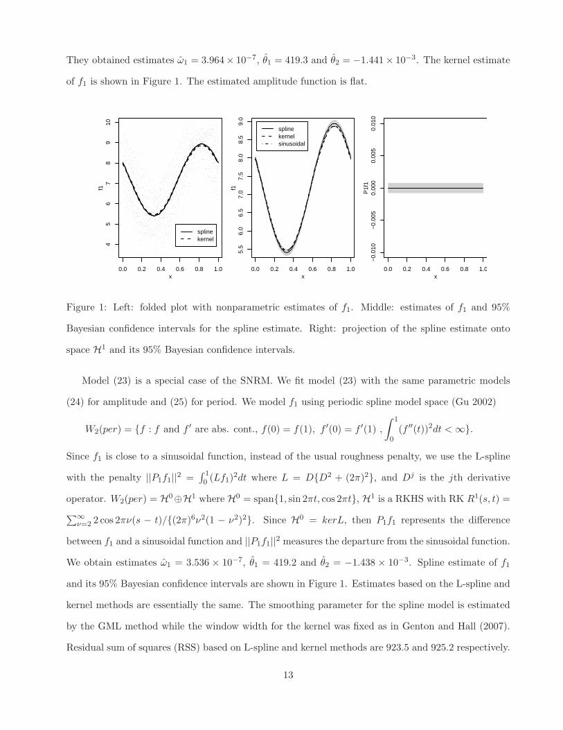
They obtained estimates ω1 = 3.964× 10−7, θ1 = 419.3 and θ2 = −1.441× 10−3. The kernel estimate

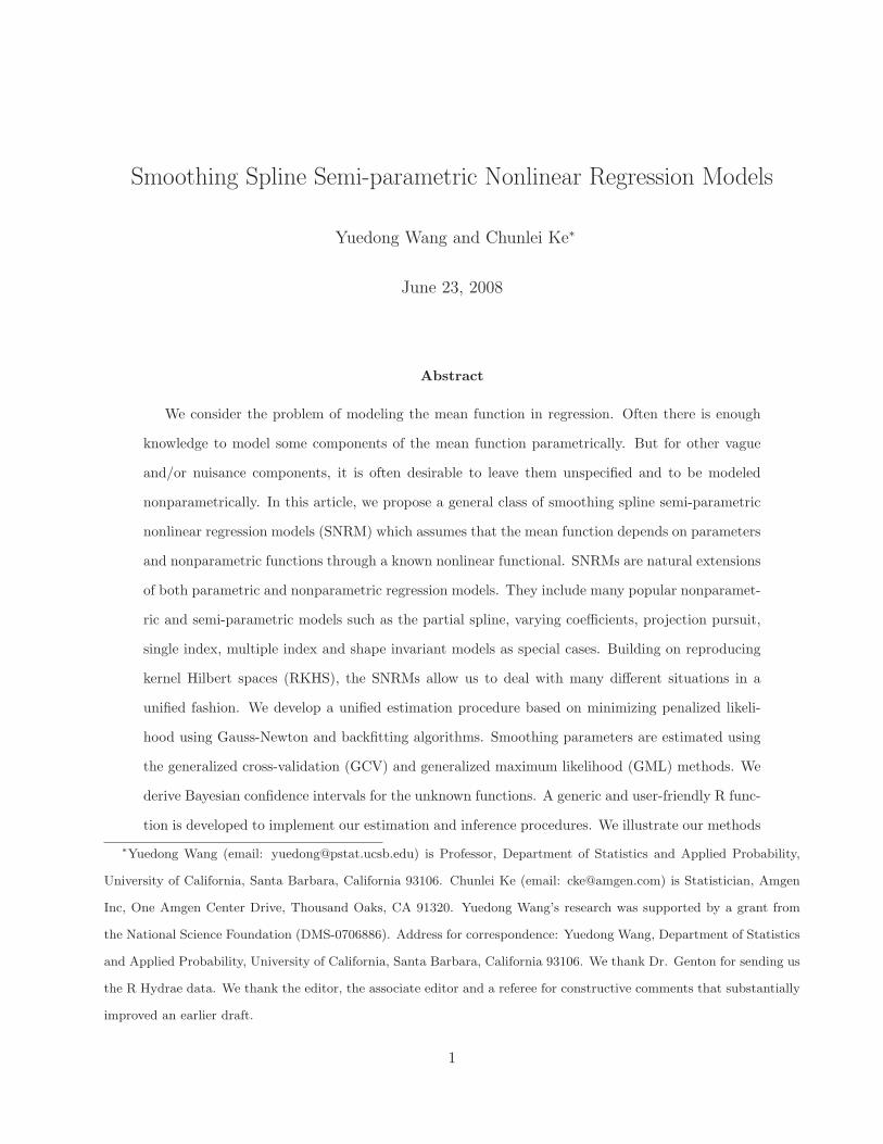
of f1 is shown in Figure 1. The estimated amplitude function is flat.

0.0 0.2 0.4 0.6 0.8 1.0

45

67

89

10

x

f1

splinekernel

0.0 0.2 0.4 0.6 0.8 1.0

5.5

6.0

6.5

7.0

7.5

8.0

8.5

9.0

x

f1

splinekernelsinusoidal

0.0 0.2 0.4 0.6 0.8 1.0

−0.

010

−0.

005

0.00

00.

005

0.01

0

x

P1f

1

Figure 1: Left: folded plot with nonparametric estimates of f1. Middle: estimates of f1 and 95%

Bayesian confidence intervals for the spline estimate. Right: projection of the spline estimate onto

space H1 and its 95% Bayesian confidence intervals.

Model (23) is a special case of the SNRM. We fit model (23) with the same parametric models

(24) for amplitude and (25) for period. We model f1 using periodic spline model space (Gu 2002)

W2(per) = {f : f and f ′ are abs. cont., f(0) = f(1), f ′(0) = f ′(1) ,

∫ 1

0(f ′′(t))2dt < ∞}.

Since f1 is close to a sinusoidal function, instead of the usual roughness penalty, we use the L-spline

with the penalty ||P1f1||2 =∫ 10 (Lf1)

2dt where L = D{D2 + (2π)2}, and Dj is the jth derivative

operator. W2(per) = H0⊕H1 where H0 = span{1, sin 2πt, cos 2πt}, H1 is a RKHS with RK R1(s, t) =

∑

∞

ν=2 2 cos 2πν(s − t)/{(2π)6ν2(1 − ν2)2}. Since H0 = kerL, then P1f1 represents the difference

between f1 and a sinusoidal function and ||P1f1||2 measures the departure from the sinusoidal function.

We obtain estimates ω1 = 3.536 × 10−7, θ1 = 419.2 and θ2 = −1.438 × 10−3. Spline estimate of f1

and its 95% Bayesian confidence intervals are shown in Figure 1. Estimates based on the L-spline and

kernel methods are essentially the same. The smoothing parameter for the spline model is estimated

by the GML method while the window width for the kernel was fixed as in Genton and Hall (2007).

Residual sum of squares (RSS) based on L-spline and kernel methods are 923.5 and 925.2 respectively.

13

The right panel in Figure 1 shows the projection of f1 onto the subspace H1, P1f1, and its 95%

Bayesian confidence intervals. The plot indicates that the function f1 is not significantly different from

a sinusoidal function since P1f1 is not significantly different from zero. We also fit a sinusoidal function

to the folded data and the estimated sinusoidal function is shown in the middle panel of Figure 1. The

sinusoidal function is inside the 95% Bayesian confidence intervals of the L-spline estimate.

Assuming the periodic shape function can be well modeled by a sinusoidal function, we can in-

vestigate evolving amplitude and period nonparametrically. This allows us to check the parametric

models in (24) and (25). We first consider the following SNRM

yi = α + exp{f2(ti)} sin[2π{β + x(ti)}] + ǫi, i = 1, · · · , n, (26)

where α is a parameter of the mean, exp{f2(ti)} is the amplitude function, β is a phase parameter

and x(t) is given in (25). Note that the exponential transformation is used to enforce the positive

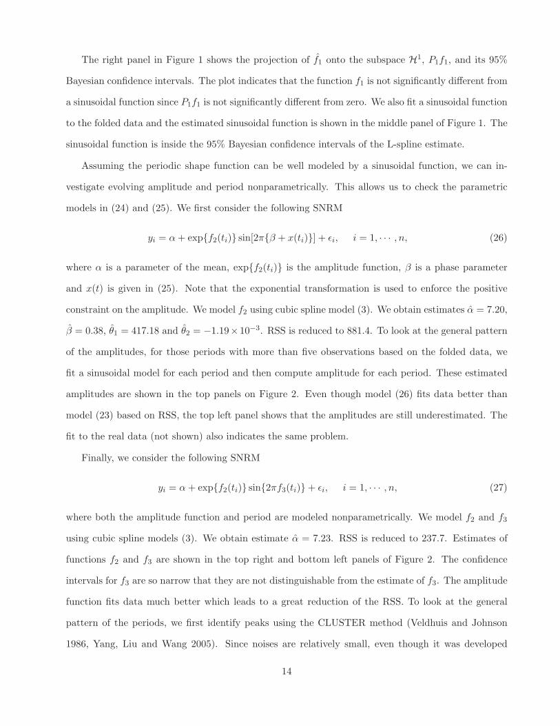
constraint on the amplitude. We model f2 using cubic spline model (3). We obtain estimates α = 7.20,

β = 0.38, θ1 = 417.18 and θ2 = −1.19×10−3. RSS is reduced to 881.4. To look at the general pattern

of the amplitudes, for those periods with more than five observations based on the folded data, we

fit a sinusoidal model for each period and then compute amplitude for each period. These estimated

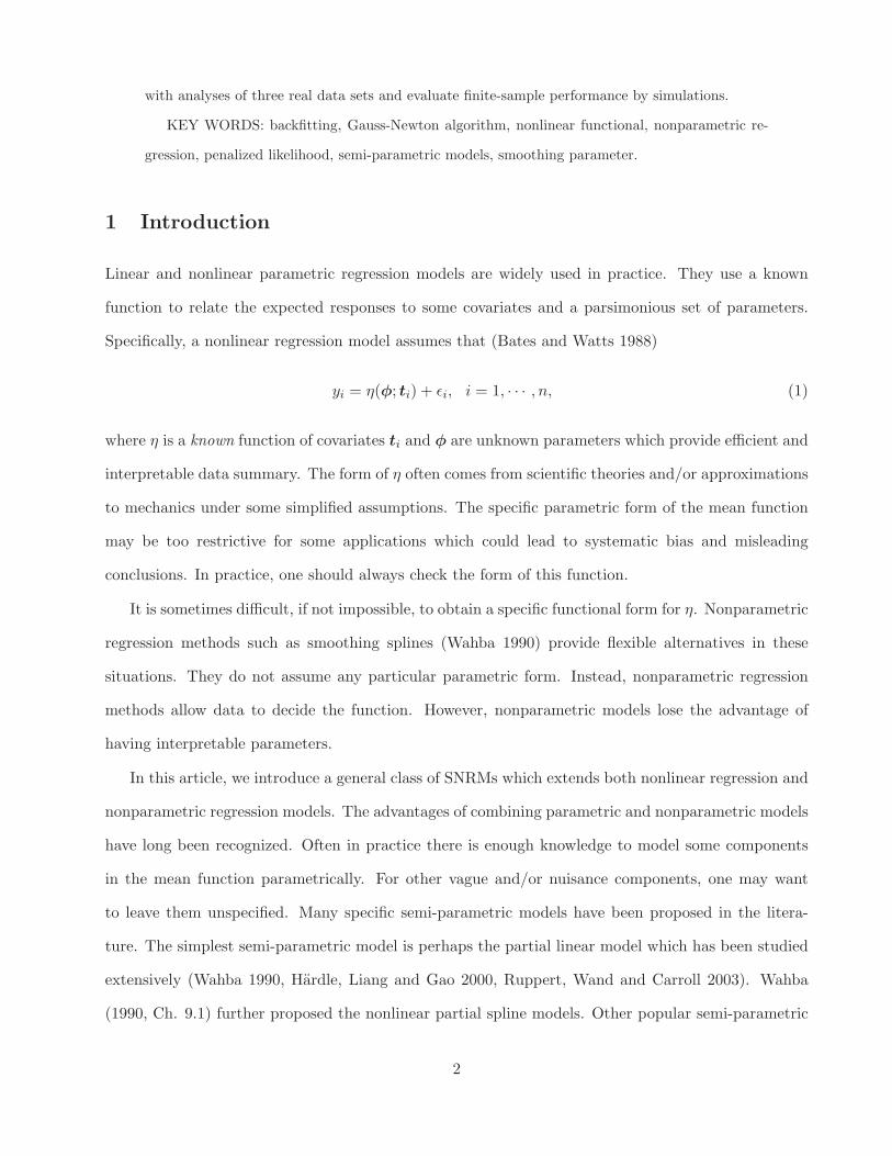
amplitudes are shown in the top panels on Figure 2. Even though model (26) fits data better than

model (23) based on RSS, the top left panel shows that the amplitudes are still underestimated. The

fit to the real data (not shown) also indicates the same problem.

Finally, we consider the following SNRM

yi = α + exp{f2(ti)} sin{2πf3(ti)} + ǫi, i = 1, · · · , n, (27)

where both the amplitude function and period are modeled nonparametrically. We model f2 and f3

using cubic spline models (3). We obtain estimate α = 7.23. RSS is reduced to 237.7. Estimates of

functions f2 and f3 are shown in the top right and bottom left panels of Figure 2. The confidence

intervals for f3 are so narrow that they are not distinguishable from the estimate of f3. The amplitude

function fits data much better which leads to a great reduction of the RSS. To look at the general

pattern of the periods, we first identify peaks using the CLUSTER method (Veldhuis and Johnson

1986, Yang, Liu and Wang 2005). Since noises are relatively small, even though it was developed

14

0 5000 10000 15000

0.0

0.2

0.4

0.6

0.8

1.0

t

f2

o

o

oo

oooo

o

o

ooo

o

o

o

oo

oo

oo

o

oo

o

o

oo

oo

o

oo

oo

o

oo

0 5000 10000 15000

0.0

0.2

0.4

0.6

0.8

1.0

t

f2

o

o

oo

oooo

o

o

ooo

o

o

o

oo

oo

oo

o

oo

o

o

oo

oo

o

oo

oo

o

oo

0 5000 10000 15000

010

2030

40

t

f3

0 5000 10000 15000

200

300

400

500

600

t

perio

d

oo

o

ooooo

o

oo

o

o

oo

o

o

o

o

ooo

o

o

oo

oo

oo

ooo

oooo

o

o

Figure 2: Top: estimated amplitudes based on folded data (circles), spline estimates of f2 based on

models (26) (left) and (27) (right), and 95% confidence intervals; bottom left: estimate of f3 based on

model (27) and its 95% Bayesian confidence intervals; bottom right: observed periods based on the

CLUSTER method (circles) and estimate of the period function 1/f ′

3(t).

for hormone pulse detection, the CLUSTER method identified peaks in the R Hydrae data with few

errors. Observed periods are estimated as the lengths between peaks. The bottom right panel of

Figure 2 shows the observed periods and the estimate of period function 1/f ′

3.

5.2 Human Growth

The dataset contains 83 measurements of height of a 10-year-old boy over one school year (Ramsay

and Silverman 2002). We are interested in the growth curve over time and its velocity. It is reasonable

to assume that the growth curve, g(t), is a monotone increasing function. Let V (t) = g′(t) be the

velocity function. While there are different ways to fit a monotone function, it is more natural to

explicitly enforce the monotonicity by assuming V (t) > 0. Rewriting V (t) = exp{f(t)}, we then can

model the function f free of constraint. The growth function g(t) = V (0) +∫ t0 V (s)ds. Therefore, we

15

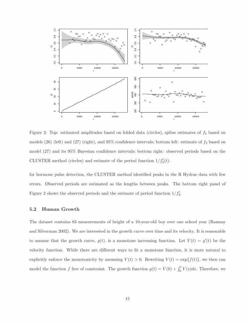
consider the following SNRM

yi = β +

∫ ti

0exp{f(t)}dt + ǫi, i = 1, · · · , 83, (28)

where yi is the height measurement in day ti. We model f using the cubic spline (3). For illustration,

we consider two error structures: (1) Independence which assumes that ǫi’s are iid and (2) AR(1) which

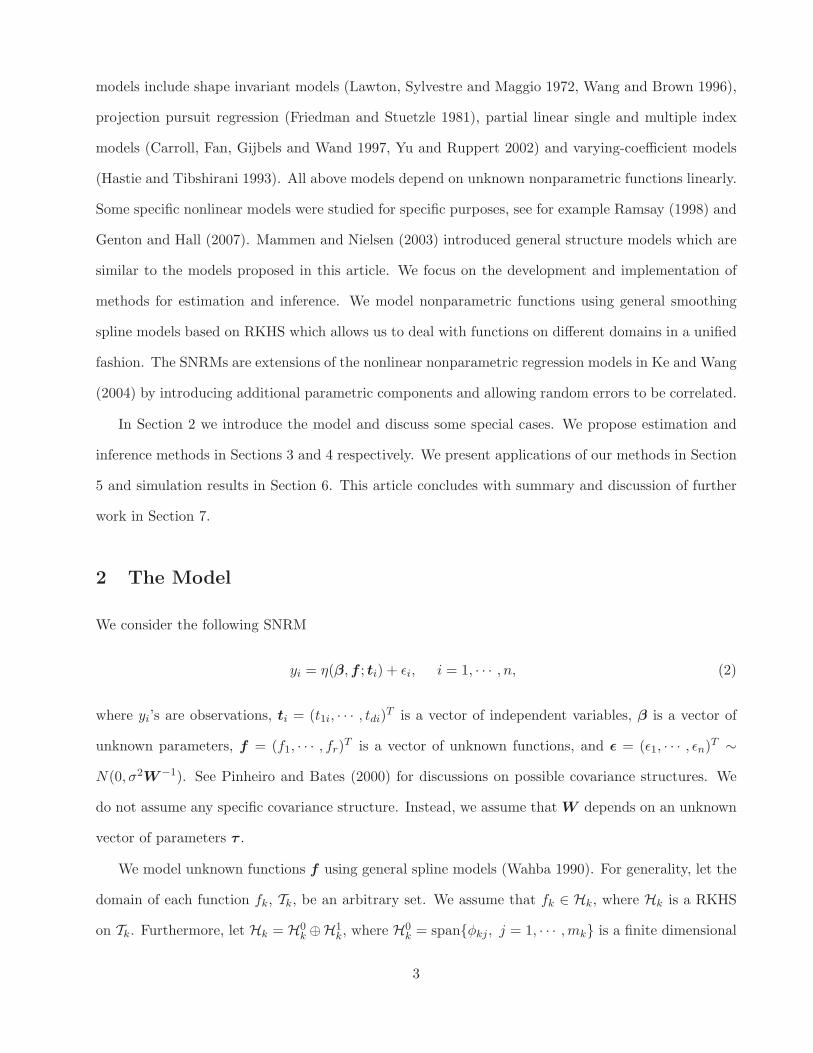
assumes that ǫi’s follow the first-order autocorrelation structure. Left panel of Figure 3 shows the

estimates of the growth curve g under two difference error structures. For comparison, we also fitted a

cubic spline for the growth function g without monotone constraint (not shown) and found that parts

of the estimate without constraint decrease. The estimate of the auto-correlation coefficient under the

AR(1) error structure is 0.78 which indicates a high auto-correlation. Note that the auto-correlation

may be part of the biological signal rather than measurement error. Estimates of the velocity are

shown on the right panel of Figure 3. The estimates of the growth curve and velocity under AR(1)

error structure are smoother.

0 50 100 150 200 250 300

124

126

128

130

Day

Hei

ght (

cm)

o

oooooooo o

o

oo

oo

oo

o

oooooo

o

o

ooo

ooo

oooooo

o

o

ooo

o

o

o

oooo

oo

o

oooooo

oooooo

ooo

oo oooo o

ooo

ooooo

IndependentAR(1)

0 50 100 150 200 250 300

0.01

0.03

0.05

Day

Gro

wth

Vel

ocity

(cm

/day

) IndependentAR(1)

Figure 3: Left: measurements of height (circles) and spline estimates. Right: estimates of growth ve-

locity and 95% bootstrap confidence intervals for the estimate under the Independence error structure

computed using the T-I method in Wang and Wahba (1996) based on 10000 bootstrap samples with

random errors sampled with replacement from residuals.

16

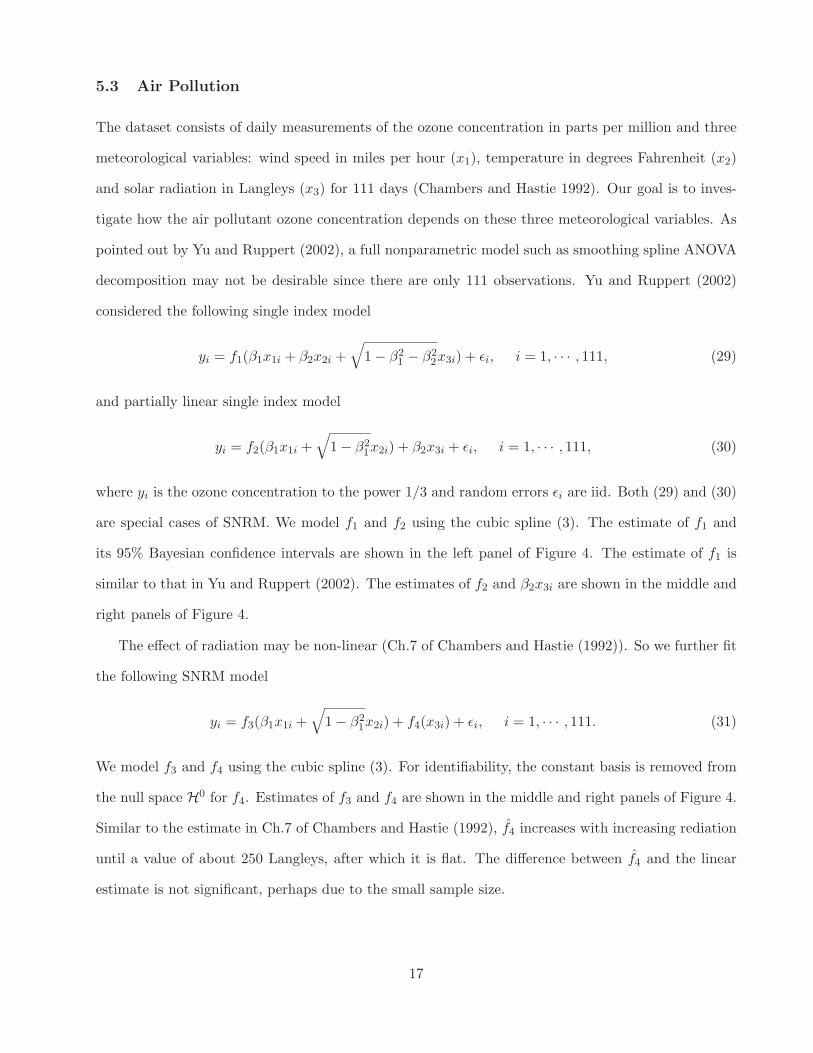
5.3 Air Pollution

The dataset consists of daily measurements of the ozone concentration in parts per million and three

meteorological variables: wind speed in miles per hour (x1), temperature in degrees Fahrenheit (x2)

and solar radiation in Langleys (x3) for 111 days (Chambers and Hastie 1992). Our goal is to inves-

tigate how the air pollutant ozone concentration depends on these three meteorological variables. As

pointed out by Yu and Ruppert (2002), a full nonparametric model such as smoothing spline ANOVA

decomposition may not be desirable since there are only 111 observations. Yu and Ruppert (2002)

considered the following single index model

yi = f1(β1x1i + β2x2i +√

1 − β21 − β2

2x3i) + ǫi, i = 1, · · · , 111, (29)

and partially linear single index model

yi = f2(β1x1i +√

1 − β21x2i) + β2x3i + ǫi, i = 1, · · · , 111, (30)

where yi is the ozone concentration to the power 1/3 and random errors ǫi are iid. Both (29) and (30)

are special cases of SNRM. We model f1 and f2 using the cubic spline (3). The estimate of f1 and

its 95% Bayesian confidence intervals are shown in the left panel of Figure 4. The estimate of f1 is

similar to that in Yu and Ruppert (2002). The estimates of f2 and β2x3i are shown in the middle and

right panels of Figure 4.

The effect of radiation may be non-linear (Ch.7 of Chambers and Hastie (1992)). So we further fit

the following SNRM model

yi = f3(β1x1i +√

1 − β21x2i) + f4(x3i) + ǫi, i = 1, · · · , 111. (31)

We model f3 and f4 using the cubic spline (3). For identifiability, the constant basis is removed from

the null space H0 for f4. Estimates of f3 and f4 are shown in the middle and right panels of Figure 4.

Similar to the estimate in Ch.7 of Chambers and Hastie (1992), f4 increases with increasing rediation

until a value of about 250 Langleys, after which it is flat. The difference between f4 and the linear

estimate is not significant, perhaps due to the small sample size.

17

20 30 40 50 60

12

34

56

Index

Con

cent

ratio

n

oo

o

oo

o

o

o

oo

oo

o

o

o

o

o

o

o

o

o

o

o

o

o

o

o

oo

o

o

o o

o

o

o

o

o

o

ooo

o

o

o

o

o

o

o

o

o

o

o

o

o

o

o

oo

o

o

o

o

o

o

o

o

o

o

o

o

o

o

o

o

o

o

o o

o

ooo

oo

o

o

o

ooo

o

o

o

o

o

o

o

o

o

o

oo

o

o

o

o

o

oo

o

20 30 40 50 60

12

34

56

IndexC

once

ntra

tion

o o

oo

o

o

o o

oo

o

o

o

o

oo

o

oo

oo

o

o

oo

o

oo

o

o o

o o

o

o

o

o

o

o

ooo

o

o

o

o

o

o

o

o

o

o

o

o

o

o

o

oo

o

o

o

o

o

o

o

o

o

o

o

oo

o

oo

o

o

o o

o

oo

o

o o

o

o

o

oo

oo

o

o

o

oo

o

ooo

o

o

oo

o

o

o

o

oo

0 50 100 200 300

−1.

5−

1.0

−0.

50.

00.

51.

01.

52.

0

Solar.R

Con

cent

ratio

n

o

o

o

o

o

o

o

o

o

o

o

o

o

o

o

o

o

o

o

o

o

o

o

o

o

o

o

o

o

o

o

o

o

o

oo

oo

o

ooo

o

o

o

oo oo

o

o

o

o

o

o o

o

o

o

o

o

o

oo

o

oo

o

o

o

o

o

o

o

o

o

o

o

o

o

oo

o

o

o

o

o

o

o

oo

o

o

o

o

o

o

oo

o

o

o

o

oo

o

o

o

o

o

o

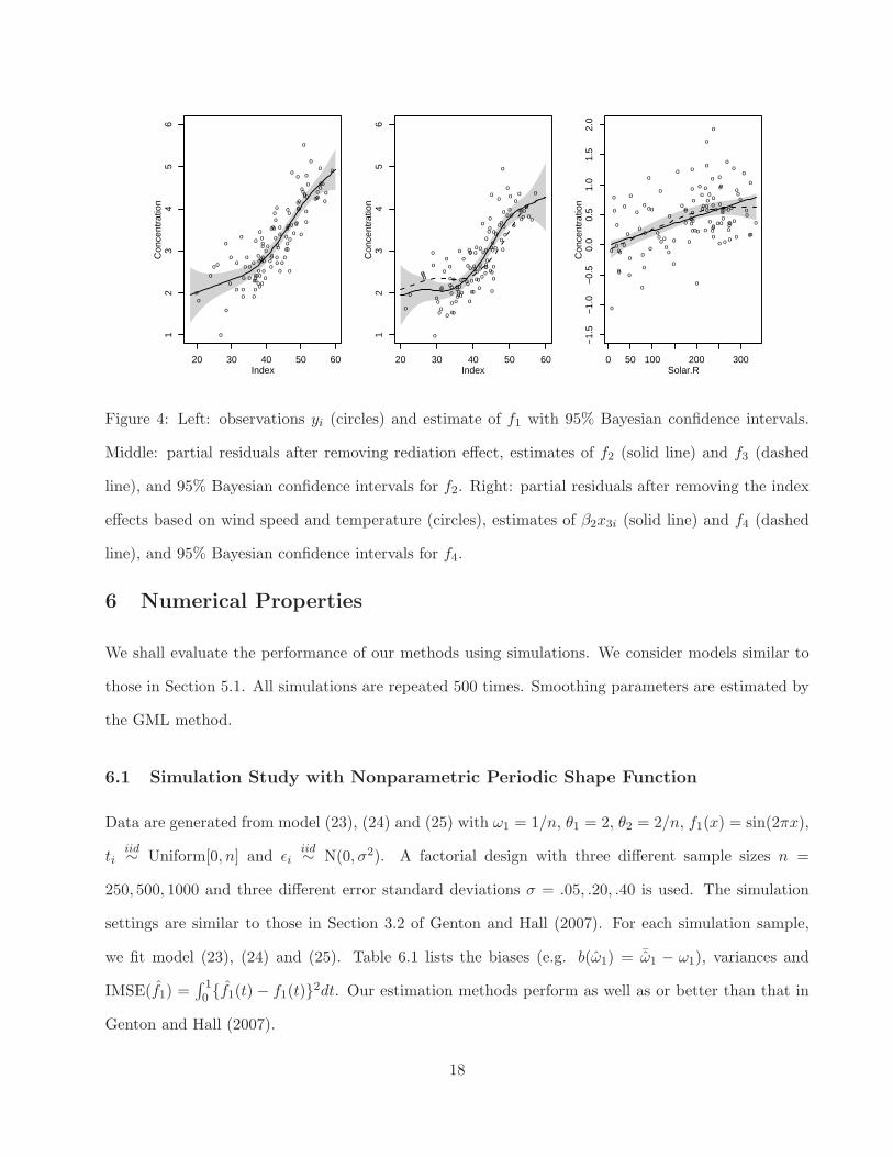
Figure 4: Left: observations yi (circles) and estimate of f1 with 95% Bayesian confidence intervals.

Middle: partial residuals after removing rediation effect, estimates of f2 (solid line) and f3 (dashed

line), and 95% Bayesian confidence intervals for f2. Right: partial residuals after removing the index

effects based on wind speed and temperature (circles), estimates of β2x3i (solid line) and f4 (dashed

line), and 95% Bayesian confidence intervals for f4.

6 Numerical Properties

We shall evaluate the performance of our methods using simulations. We consider models similar to

those in Section 5.1. All simulations are repeated 500 times. Smoothing parameters are estimated by

the GML method.

6.1 Simulation Study with Nonparametric Periodic Shape Function

Data are generated from model (23), (24) and (25) with ω1 = 1/n, θ1 = 2, θ2 = 2/n, f1(x) = sin(2πx),

tiiid∼ Uniform[0, n] and ǫi

iid∼ N(0, σ2). A factorial design with three different sample sizes n =

250, 500, 1000 and three different error standard deviations σ = .05, .20, .40 is used. The simulation

settings are similar to those in Section 3.2 of Genton and Hall (2007). For each simulation sample,

we fit model (23), (24) and (25). Table 6.1 lists the biases (e.g. b(ω1) = ¯ω1 − ω1), variances and

IMSE(f1) =∫ 10 {f1(t) − f1(t)}2dt. Our estimation methods perform as well as or better than that in

Genton and Hall (2007).

18

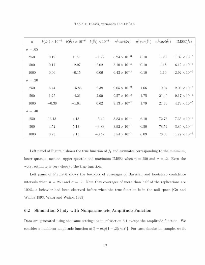
Table 1: Biases, variances and IMSEs.

n b(ω1) × 10−6 b(θ1) × 10−6 b(θ2) × 10−8 n3var(ω1) n3var(θ1) n5var(θ2) IMSE(f1)

σ = .05

250 0.19 1.62 −1.92 6.24 × 10−3 0.10 1.20 1.09 × 10−5

500 0.17 −2.97 2.02 5.10 × 10−3 0.10 1.18 6.12 × 10−6

1000 0.06 −0.15 0.06 6.43 × 10−3 0.10 1.19 2.92 × 10−6

σ = .20

250 6.44 −15.85 2.38 9.05 × 10−2 1.66 19.94 2.06 × 10−4

500 1.25 −4.21 2.90 9.57 × 10−2 1.75 21.40 9.17 × 10−5

1000 −0.36 −1.64 0.62 9.13 × 10−2 1.79 21.30 4.73 × 10−5

σ = .40

250 13.13 4.13 −5.49 3.83 × 10−1 6.10 72.73 7.35 × 10−4

500 4.52 5.13 −3.83 3.92 × 10−1 6.50 78.54 3.86 × 10−4

1000 0.23 2.13 −0.47 3.54 × 10−1 6.09 73.00 1.77 × 10−4

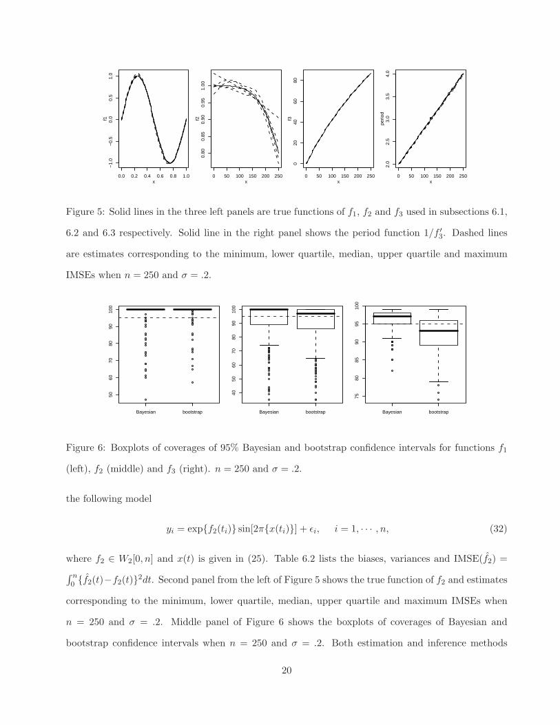
Left panel of Figure 5 shows the true function of f1 and estimates corresponding to the minimum,

lower quartile, median, upper quartile and maximum IMSEs when n = 250 and σ = .2. Even the

worst estimate is very close to the true function.

Left panel of Figure 6 shows the boxplots of coverages of Bayesian and bootstrap confidence

intervals when n = 250 and σ = .2. Note that coverages of more than half of the replications are

100%, a behavior had been observed before when the true function is in the null space (Gu and

Wahba 1993, Wang and Wahba 1995)

6.2 Simulation Study with Nonparametric Amplitude Function

Data are generated using the same settings as in subsection 6.1 except the amplitude function. We

consider a nonlinear amplitude function a(t) = exp{1 − .2(t/n)4}. For each simulation sample, we fit

19

0.0 0.2 0.4 0.6 0.8 1.0

−1.

0−

0.5

0.0

0.5

1.0

x

f1

0 50 100 150 200 250

0.80

0.85

0.90

0.95

1.00

x

f2

0 50 100 150 200 250

020

4060

80

x

f3

0 50 100 150 200 250

2.0

2.5

3.0

3.5

4.0

x

perio

d

Figure 5: Solid lines in the three left panels are true functions of f1, f2 and f3 used in subsections 6.1,

6.2 and 6.3 respectively. Solid line in the right panel shows the period function 1/f ′

3. Dashed lines

are estimates corresponding to the minimum, lower quartile, median, upper quartile and maximum

IMSEs when n = 250 and σ = .2.

Bayesian bootstrap

5060

7080

9010

0

Bayesian bootstrap

4050

6070

8090

100

Bayesian bootstrap

7580

8590

9510

0

Figure 6: Boxplots of coverages of 95% Bayesian and bootstrap confidence intervals for functions f1

(left), f2 (middle) and f3 (right). n = 250 and σ = .2.

the following model

yi = exp{f2(ti)} sin[2π{x(ti)}] + ǫi, i = 1, · · · , n, (32)

where f2 ∈ W2[0, n] and x(t) is given in (25). Table 6.2 lists the biases, variances and IMSE(f2) =

∫ n0 {f2(t)−f2(t)}2dt. Second panel from the left of Figure 5 shows the true function of f2 and estimates

corresponding to the minimum, lower quartile, median, upper quartile and maximum IMSEs when

n = 250 and σ = .2. Middle panel of Figure 6 shows the boxplots of coverages of Bayesian and

bootstrap confidence intervals when n = 250 and σ = .2. Both estimation and inference methods

20

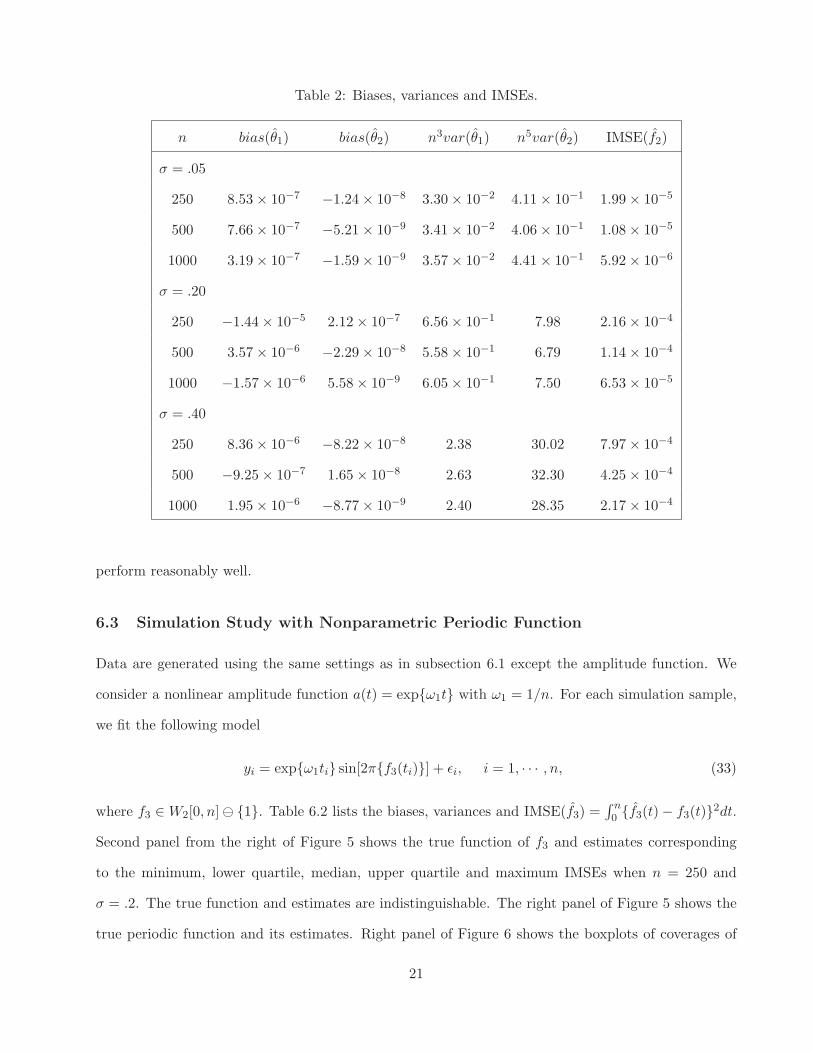
Table 2: Biases, variances and IMSEs.

n bias(θ1) bias(θ2) n3var(θ1) n5var(θ2) IMSE(f2)

σ = .05

250 8.53 × 10−7 −1.24 × 10−8 3.30 × 10−2 4.11 × 10−1 1.99 × 10−5

500 7.66 × 10−7 −5.21 × 10−9 3.41 × 10−2 4.06 × 10−1 1.08 × 10−5

1000 3.19 × 10−7 −1.59 × 10−9 3.57 × 10−2 4.41 × 10−1 5.92 × 10−6

σ = .20

250 −1.44 × 10−5 2.12 × 10−7 6.56 × 10−1 7.98 2.16 × 10−4

500 3.57 × 10−6 −2.29 × 10−8 5.58 × 10−1 6.79 1.14 × 10−4

1000 −1.57 × 10−6 5.58 × 10−9 6.05 × 10−1 7.50 6.53 × 10−5

σ = .40

250 8.36 × 10−6 −8.22 × 10−8 2.38 30.02 7.97 × 10−4

500 −9.25 × 10−7 1.65 × 10−8 2.63 32.30 4.25 × 10−4

1000 1.95 × 10−6 −8.77 × 10−9 2.40 28.35 2.17 × 10−4

perform reasonably well.

6.3 Simulation Study with Nonparametric Periodic Function

Data are generated using the same settings as in subsection 6.1 except the amplitude function. We

consider a nonlinear amplitude function a(t) = exp{ω1t} with ω1 = 1/n. For each simulation sample,

we fit the following model

yi = exp{ω1ti} sin[2π{f3(ti)}] + ǫi, i = 1, · · · , n, (33)

where f3 ∈ W2[0, n] ⊖ {1}. Table 6.2 lists the biases, variances and IMSE(f3) =∫ n0 {f3(t) − f3(t)}2dt.

Second panel from the right of Figure 5 shows the true function of f3 and estimates corresponding

to the minimum, lower quartile, median, upper quartile and maximum IMSEs when n = 250 and

σ = .2. The true function and estimates are indistinguishable. The right panel of Figure 5 shows the

true periodic function and its estimates. Right panel of Figure 6 shows the boxplots of coverages of

21

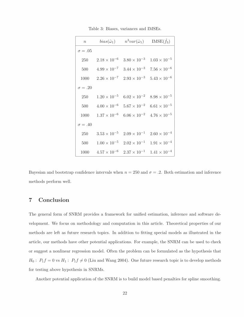
Table 3: Biases, variances and IMSEs.

n bias(ω1) n3var(ω1) IMSE(f3)

σ = .05

250 2.18 × 10−6 3.80 × 10−3 1.03 × 10−5

500 4.99 × 10−7 3.44 × 10−3 7.56 × 10−6

1000 2.26 × 10−7 2.93 × 10−3 5.43 × 10−6

σ = .20

250 1.20 × 10−5 6.02 × 10−2 8.98 × 10−5

500 4.00 × 10−6 5.67 × 10−2 6.61 × 10−5

1000 1.37 × 10−6 6.06 × 10−2 4.76 × 10−5

σ = .40

250 3.53 × 10−5 2.09 × 10−1 2.60 × 10−4

500 1.00 × 10−5 2.02 × 10−1 1.91 × 10−4

1000 4.57 × 10−6 2.37 × 10−1 1.41 × 10−4

Bayesian and bootstrap confidence intervals when n = 250 and σ = .2. Both estimation and inference

methods perform well.

7 Conclusion

The general form of SNRM provides a framework for unified estimation, inference and software de-

velopment. We focus on methodology and computation in this article. Theoretical properties of our

methods are left as future research topics. In addition to fitting special models as illustrated in the

article, our methods have other potential applications. For example, the SNRM can be used to check

or suggest a nonlinear regression model. Often the problem can be formulated as the hypothesis that

H0 : P1f = 0 vs H1 : P1f 6= 0 (Liu and Wang 2004). One future research topic is to develop methods

for testing above hypothesis in SNRMs.

Another potential application of the SNRM is to build model based penalties for spline smoothing.

22

The model space H, its decomposition H = H0 ⊕ H1 and the penalty ||P1f ||2 are usually fixed

when fitting smoothing spline models (Wahba 1990, Gu 2002). Nevertheless, Heckman and Ramsay

(2000) showed that appropriate choice of the model space and its decomposition may involve unknown

parameters in the penalty functional. Often, this problem of fitting smoothing spline with unknown

parameters in the penalty functional is equivalent to fitting a SNRM.

A closely related field is linear and nonlinear inverse problems. As a result of the interaction of

a physical system, a function f is observed through the transformation T (f) where T is a linear or

nonlinear operator. The goal is to recover the function f through data. Sometimes the operator

T depends on some unknown parameters (Esedoglu 2004, Pillonetto and Bell 2004) which lead to

SNRMs. Inverse problems are often ill-posed and regularization is the common approach which is

equivalent to the penalized likelihood method when data are observed with random errors. Thus our

methods provide an alternative approach for nonlinear inverse problems with data driven choices of

regularization parameters.

In this article we are interested in the estimation and inference for both parameters and nonpara-

metric functions. When the parameters are of main interest, for linear semi-parametric models, it

is well-known that optimal rate of convergence for parameters can be achieved by using the profile

likelihood (Speckman 1988, Severini and Wong 1992, Severini and Staniswalis 1994). Whether these

results can be extended to nonlinear semi-parametric models proposed in this article remains an open

problem.

References

Aronszajn, N. (1950). Theory of reproducing kernels, Trans. Amer. Math. Soc. 68: 337–404.

Bates, D. M. and Watts, D. G. (1988). Nonlinear Regression Analysis and Its Applications, Wiley.

Carroll, R. J., Fan, J., Gijbels, I. and Wand, M. P. (1997). Generalized partial linear single-index

models, Journal of the American Statistical Association 92: 477–489.

Chambers, J. and Hastie, T. (1992). Statistical Models in S, Wadsworth and Brooks.

23

Esedoglu, S. (2004). Blind deconvolution of bar code signals, Inverse Problems 20: 121–135.

Flett, T. M. (1980). Differential Analysis, Cambridge University Press, London.

Friedman, J. H. and Stuetzle, W. (1981). Projection pursuit regression, Journal of the American

Statistical Association 76: 817–823.

Genton, M. G. and Hall, P. (2007). Statistical inference for envolving periodic functions, Journal of

the Royal Statistical Society B 69: 643–657.

Gu, C. (1989). RKPACK and its applications: Fitting smoothing spline models, Proceedings of the

Statistical Computing Section, ASA: pp. 42–51.

Gu, C. (2002). Smoothing Spline ANOVA Models, Springer-Verlag, New York.

Gu, C. and Wahba, G. (1993). Smoothing spline ANOVA with component-wise Bayesian confidence

intervals, Journal of Computational and Graphical Statistics 2: 97–117.

Hardle, W., Liang, H. and Gao, J. (2000). Partial linear Models, Springer-Verlag, New York.

Hastie, T. and Tibshirani, R. (1993). Varying coefficient model, Journal of the Royal Statistical Society

B 55: 757–796.

Heckman, N. and Ramsay, J. O. (2000). Penalized regression with model-based penalties, Canadian

Journal of Statistics 28: 241–258.

Ke, C. and Wang, Y. (2004). Nonparametric nonlinear regression models, Journal of the American

Statistical Association 99: 1166–1175.

Lawton, W. H., Sylvestre, E. A. and Maggio, M. S. (1972). Self-modeling nonlinear regression, Tech-

nometrics 13: 513–532.

Liu, A. and Wang, Y. (2004). Hypothesis testing in smoothing spline models, Journal of Statistical

Computation and Simulation 74: 581–597.

Mammen, E. and Nielsen, J. P. (2003). Generalised structured models, Biometrika 90: 551–566.

24

Pillonetto, G. and Bell, B. M. (2004). Deconvolution of non-stationary physical signals: a smooth

variance model for insulin secretion rate, Inverse Problems 20: 367–383.

Pinheiro, J. and Bates, D. M. (2000). Mixed-effects Models in S and S-plus, Springer, New York.

Ramsay, J. O. (1998). Estimating smooth monotone functions, Journal of the Royal Statistical Society

B 60: 365–375.

Ramsay, J. O. and Silverman, B. W. (2002). Applied Functional Data Analysis, Springer, New York.

Ruppert, D., Wand, M. P. and Carroll, R. J. (2003). Semiparametric Regression, Cambridge, New

York.

Severini, T. and Staniswalis, J. (1994). Quasi-likelihood estimation in semiparametric models, Journal

of the American Statistical Association 89: 501–511.

Severini, T. and Wong, W. (1992). Generalized profile likelihood and conditional parametric models,

Annals of Statistics 20: 1768–1802.

Speckman, P. (1988). Kernel-smoothing in partial linear models, Journal of the Royal Statistical

Society B 50: 413–436.

Veldhuis, J. D. and Johnson, M. L. (1986). Cluster analysis: a simple versatile and robust algorithm

for endocrine pulse detection, American Journal of Physiology 250: E486–E493.

Wahba, G. (1978). Improper priors, spline smoothing, and the problem of guarding against model

errors in regression, Journal of the Royal Statistical Society B 40: 364–372.

Wahba, G. (1990). Spline Models for Observational Data, SIAM, Philadelphia. CBMS-NSF Regional

Conference Series in Applied Mathematics, Vol. 59.

Wahba, G., Wang, Y., Gu, C., Klein, R. and Klein, B. (1995). Smoothing spline ANOVA for exponen-

tial families, with application to the Wisconsin Epidemiological Study of Diabetic Retinopathy,

Annals of Statistics 23: 1865–1895.

25

Wang, Y. (1998). Smoothing spline models with correlated random errors, Journal of the American

Statistical Association 93: 341–348.

Wang, Y. and Brown, M. B. (1996). A flexible model for human circadian rhythms, Biometrics

52: 588–596.

Wang, Y. and Wahba, G. (1995). Bootstrap confidence intervals for smoothing splines and their

comparison to Bayesian confidence intervals, J. Statist. Comput. Simul. 51: 263–279.

Yang, Y., Liu, A. and Wang, Y. (2005). Detecting pulsatile hormone secretions using nonlinear mixed

effects partial spline models, Biometrics pp. 230–238.

Yu, Y. and Ruppert, D. (2002). Penalized spline estimation for partially linear single index models,

Journal of the American Statistical Association 97: 1042–1054.

Zijlstra, A., Bedding, T. and Mattei, J. (2002). The evolution of the mira variable R Hydrae, Monthly

Notices of the Royal Astronomical Society 334: 498–510.

Appendix: Derivation of Posterior Covariances

Let y = z + ǫ where z ∼ N(0, bΣz,z), ǫ ∼ N(0, σ2W−1) and E(zǫT ) = 0. Let g and h be zero

mean Gaussian random vectors such that E(ghT ) = bΣg,h E(gzT ) = bΣg,z and E(zhT ) = bΣz,h. Let

σ2/b = nλ. Then (Gu and Wahba, 1993)

1

bCov(g, h|y) = Σg,h − Σg,z(Σz,z + nλW )−1Σz,h. (A.1)

Now suppose that we want to compute the posterior covariance between Fj(sj) and Fk(tk). Let

g = Fj(sj), h = Fk(tk) and z = (∑r

k=1 Lk1Fk, · · · ,∑r

k=1 LknFk)T . By the correspondence between

H1k and the Hilbert space spanned by Xk(tk) (Wahba 1990, Ch. 1.4), we have

E(LkiXk)Xk(tk) = Lki(·)R1k(tk, ·) = ξki(tk),

E(LkiXk)(LkjXk) = Lki(·)Lkj(·)R1k.

26

Let Xk = (Lk1Xk, · · · ,LknXk)T . Then EXkXk(tk) = (ξk1(tk), · · · , ξkn(tk))

T = ξk(tk) and

E(zT z) = b(ρTT T + Σ),

E(gh) = {amk∑

ν=1

φkν(sk)φkν(tk) + bθkR1k(sk, tk)}I(j = k)

= b{

ρφTk (sk)φk(tk) + θkR

1k(sk, tk)

}

I(j = k),

E(gzT ) = E{

φTj (sj)ζj +

√

bθjXj(sj)} {

ζTj T T

j +√

bθjXTj

}

= b{

ρφTj (sj)T

Tj + θjξ

Tj (sj)

}

,

E(zh) = E{

T kζk +√

bθkXk

} {

ζTk φk(tk) +

√

bθkXk(tk)}

= b {ρT kφk(tk) + θkξk(tk)} , (A.2)

where ρ = a/b, ζk = (ζk1, · · · , ζkmk)T and φk(tk) = (φk1(tk), · · · , φkmk

(tk))T . It is easy to show that

formulae (A.4) in Gu and Wahba (1993) hold with M = Σ + nλW−1 for correlated data. Plugging

(A.2) back in (A.1), we then have

1

bCov{Fj(sj), Fk(tk)|y}

= {ρφTk (sk)φk(tk) + θkR

1k(sk, tk)}I(j = k)

−{ρφTj (sj)T

Tj + θjξ

Tj (sj)}(ρTT T + M)−1{ρT kφk(tk) + θkξk(tk)}

= φTj (sj){ρI(j = k)I − ρT T

j (ρTT T + M)−1ρT k}φk(tk)

−ρφTj (sj)T

Tj (ρTT T + M)−1θkξk(tk)

−θjξTj (sj)(ρTT T + M)−1ρT kφk(tk) + θkR

1k(sk, tk)I(j = k)

−θjθkξTj (sj)(ρTT T + M)−1ξk(tk)

ρ→∞→ φTj (sj)U jkφk(tk) − φT

j (sj)V k(tk) − V Tj (sj)φk(tk) + θkR

1k(sk, tk)I(j = k)

−θjθkξTj (sj){M−1 − M−1T T (T T M−1T )−1T T M−1}ξk(tk),

where U jk is a mj ×mk matrix corresponds to rows∑j−1

l=1 ml +1 to∑j

l=1 ml and columns∑k−1

l=1 ml +1

to∑k

l=1 ml of the matrix (T T M−1T )−1, and V k(tk) is a subvector of (T T M−1T )−1T T M−1ξk(tk)

with elements from∑k−1

l=1 ml + 1 to∑k

l=1 ml.

Since g0jν(sj), gj(sj), g0

kµ(tk) and gk(tk) in (21) correspond to some components in Fj(sj) and

Fk(tk), posterior covariances in (21) can be derived similarly by picking up corresponding components.

27